| Issue |
A&A
Volume 547, November 2012
|
|
|---|---|---|
| Article Number | A49 | |
| Number of page(s) | 79 | |
| Section | Galactic structure, stellar clusters and populations | |
| DOI | https://doi.org/10.1051/0004-6361/201219232 | |
| Published online | 26 October 2012 | |
The Earliest Phases of Star Formation (EPoS): a Herschel⋆ key program
The precursors to high-mass stars and clusters⋆⋆
1
Max-Planck-Institute for Astronomy, Königstuhl 17, 69117
Heidelberg,
Germany
e-mail: This email address is being protected from spambots. You need JavaScript enabled to view it.
2
AIM Paris-Saclay, CEA/DSM/IRFU – CNRS/INSU – Université Paris
Diderot, CEA Saclay, 91191
Gif-sur-Yvette Cedex,
France
3
Universität zu Köln, Zülpicher Strasse 77, 50937
Köln,
Germany
4
Max-Planck-Institut für Radioastronomie,
Auf dem Hügel 69,
53121
Bonn,
Germany
5
Institut de Planétologie et
d′Astrophysique de Grenoble,
414 rue de la Piscine, 38400 St-Martin d′Hères, France
6
Department of Chemistry, Astronomy and Physics, University of
Virginia, Charlottesville, VA
22904,
USA
Received:
16
March
2012
Accepted:
27
July
2012
Abstract
Context. Stars are born deeply embedded in molecular clouds. In the earliest embedded phases, protostars emit the bulk of their radiation in the far-infrared wavelength range, where Herschel is perfectly suited to probe at high angular resolution and dynamic range. In the high-mass regime, the birthplaces of protostars are thought to be in the high-density structures known as infrared-dark clouds (IRDCs). While massive IRDCs are believed to have the right conditions to give rise to massive stars and clusters, the evolutionary sequence of this process is not well-characterized.
Aims. As part of the Earliest Phases of Star formation (EPoS) Herschel guaranteed time key program, we isolate the embedded structures within IRDCs and other cold, massive molecular clouds. We present the full sample of 45 high-mass regions which were mapped at PACS 70, 100, and 160 μm and SPIRE 250, 350, and 500 μm. In the present paper, we characterize a population of cores which appear in the PACS bands and place them into context with their host molecular cloud and investigate their evolutionary stage.
Methods. We construct spectral energy distributions (SEDs) of 496 cores which appear in all PACS bands, 34% of which lack counterparts at 24 μm. From single-temperature modified blackbody fits of the SEDs, we derive the temperature, luminosity, and mass of each core. These properties predominantly reflect the conditions in the cold, outer regions. Taking into account optical depth effects and performing simple radiative transfer models, we explore the origin of emission at PACS wavelengths.
Results. The core population has a median temperature of 20 K and has masses and luminosities that span four to five orders of magnitude. Cores with a counterpart at 24 μm are warmer and bluer on average than cores without a 24 μm counterpart. We conclude that cores bright at 24 μm are on average more advanced in their evolution, where a central protostar(s) have heated the outer bulk of the core, than 24 μm-dark cores. The 24 μm emission itself can arise in instances where our line of sight aligns with an exposed part of the warm inner core. About 10% of the total cloud mass is found in a given cloud’s core population. We uncover over 300 further candidate cores which are dark until 100 μm. These are possibly starless objects, and further observations will help us determine the nature of these very cold cores.
Key words: stars: formation / stars: protostars / stars: massive / techniques: photometric
Herschel is an ESA space observatory with science instruments provided by European-led Principal Investigator consortia and with important participation from NASA.
Appendices are available in electronic form at http://www.aanda.org
© ESO, 2012
1. Introduction
Star formation is a critical ingredient in a broad range of astrophysical phenomena, yet there are fundamental components of the process – particularly in the early stages – that remain poorly understood. Over the past decades, a basic framework for the formation of low-mass stars has developed beginning with gravitationally bound pre-stellar cores (Ward-Thompson et al. 2002), evolving into Class 0 and Class I protostars then Class II and Class III pre-main sequence stars (Shu et al. 1987; André et al. 1993). Such a sequence for the formation of high-mass stars has not yet been established. Several good candidates for massive young cores have been identified using the 170 μm ISOPHOT Serendipity Survey (ISOSS) (Lemke et al. 1996; Krause et al. 2003, 2004; Birkmann et al. 2006) or sensitive millimeter surveys (e.g. Klein et al. 2005; Sridharan et al. 2005). However, upon further investigation, most have been found to already host (deeply embedded) low- to intermediate-mass protostars (e.g. Motte et al. 2007; Hennemann et al. 2008; Beuther & Henning 2009). It is the stage previous to the onset of massive protostar formation that continues to elude observers.
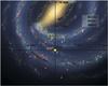 |
Fig. 1 Face-on schematic view of the distribution of IRDCs (green triangles) and ISOSS sources (red squares) and the HMSC 07029 (blue triangle) in the Milky Way. The background image is an artist’s impression of the Milky Way based on the GLIMPSE survey, credit R. Hurt [SSC-Caltech], adapted by MPIA graphics department. The kinematic distances to each object are derived using the Reid et al. (2009) model. |
Many gaps remain in our understanding of how massive stars and clusters form, beginning with the elusive initial conditions. Do massive stars result from the gravitational collapse of cold, very massive cores (Evans et al. 2002; Beuther et al. 2007) like their low-mass siblings? What role does the environment play in determining the ultimate fate of such cores? As a (massive) protostar evolves, how drastically do its properties change, and what impact does it have on its surroundings? In order to study these very early, embedded phases of (massive) star formation, access to the far-infrared wavelength regime, where the peak of the cold dust radiation (Tdust ~ 10−20 K) is located, is critical. In addition, high angular resolution is needed to study massive star-forming regions which usually reside several kiloparsecs from the Sun. The Herschel far-infrared satellite (Pilbratt et al. 2010) drastically improves our ability to peer deep into the dense regions where such young cores are embedded.
The Earliest Phases of Star formation (EPoS) guaranteed time key program (P.I. O. Krause; Henning et al. 2010; Linz et al. 2010; Beuther et al. 2010; Stutz et al. 2010) is a PACS and SPIRE photometric mapping survey which targets objects known to be in the cold early phases of star formation. There are two main components to the EPoS sample: 15 isolated, low-mass globules at various evolutionary stages, from starless to Class I, and 45 high-mass regions, which are mostly larger, high density molecular cloud complexes containing a range of objects within their boundaries. In Stutz et al. (2010), Nielbock et al. (2012), and a forthcoming comprehensive study by Launhardt et al. (in prep.), the low-mass part of the EPoS sample is investigated. In this overview, we focus on the high-mass star-forming regions.
Our sample is comprised of objects known as infrared-dark clouds (IRDCs), which were first discovered in silhouette against the bright Galactic background in the mid-infrared with the ISOCAM instrument (Perault et al. 1996) and the MSX satellite (Egan et al. 1998) at 15 and 8 μm, respectively. Several surveys in millimeter and sub-millimeter continuum and spectral lines have followed (e.g. Carey et al. 1998, 2000; Teyssier et al. 2002; Pillai et al. 2006a; Rathborne et al. 2006; Ragan et al. 2006; Vasyunina et al. 2009) and have established that massive IRDCs harbor the precursors and early phases of massive star and cluster formation. We select 29 IRDCs, most of which are in the inner quadrants of the Galaxy (see Fig. 1). Assuming the IRDCs lie on the near side of the Milky Way (see Sect. 2.2), they coincide with the Scutum-Centraurus spiral arm, which (in the first quadrant) overlaps with the Molecular Ring (Jackson et al. 2008). Also part of our sample are sources discovered in the ISO Serendipity Survey (ISOSS) at 170 μm, which are seen to harbor cold, massive clumps at large Galactocentric distances.
We present the first comprehensive results of the Herschel PACS and SPIRE imaging survey of 45 massive targets as part of the EPoS survey. The goals of this study are as follows: (1) give a general characterization of the sample based on Herschel data in concert with existing complementary datasets; (2) characterize point sources embedded within the targeted clouds; and (3) connect the point source properties to the overall cloud structure and environment.
2. Sample description
2.1. Target selection
The high-mass portion of EPoS guaranteed time key program sample was compiled from several different surveys with varying approaches, but they are unified in that insofar as the existing data show, they are all candidates to be in the earliest stages of high-mass star formation. Table 3 summarizes our targets, with their positions, distances, and mass estimates from various Galactic plane survey data which we will detail below. Appendix A describes the selection strategy and each of the individual sources in greater detail.
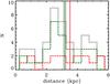 |
Fig. 2 Histogram of distances of the 45 clouds in the sample in 0.5 kpc bins. The full sample is plotted in the solid gray histogram, the histogram for just the IRDCs is plotted in the green dot-dashed line, and the ISOSS targets are plotted in the red histogram. The median distance of the full sample, 3.2 kpc, is plotted in the solid gray line, and the median for the IRDC-only (3.1 kpc) and ISOSS-only (3.5 kpc) are shown with solid green and red vertical lines. |
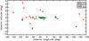 |
Fig. 3 Galactic distribution of EPoS high-mass sample in Galactic latitude and longitude. Green triangles represent IRDCs and red squares represent ISOSS sources. The blue triangle is HMSC 07029. |
2.2. Distances and Galactic distribution
We derive kinematic distances for each of the IRDCs following the method put forward in Reid et al. (2009), adopting the updated distance to the Galactic Center of R0 = 8.4 kpc and a circular rotation speed of Θ0 = 254 km s-1. Table 3 lists the vlsr that was used, the reference from which this velocity was obtained, and the resulting distances and uncertainties, assuming the recommended 7 km s-1 uncertainty in vlsr, the source of which is listed in the References column of Table 3. We show the distribution of distances in Fig. 2. The overall median distance is 3.2 kpc. We also show that the median distance to “classical” IRDCs (3.1 kpc) is only slightly smaller than that of the ISOSS portion of the sample, 3.5 kpc. Considering the typical distance uncertainties, these subsamples occupy equivalent distance ranges.
We show the spatial distribution of the targets throughout the Galaxy in Figs. 3 and 1. Only a small fraction of the sources lie outside ± 1° in Galactic latitude, and we see in Fig. 3 that the farthest outliers tend to be the ISOSS sources. As shown in Fig. 1, the majority of the well-studied IRDCs lie in the first quadrant, coincident with the Scutum-Centaurus spiral arm. On the other hand, the ISOSS sources appear to coincide with the Sagittarius arm (in the first quadrant) or the Perseus arm (in the outer Galaxy).
2.3. Ancillary data
2.3.1. Mid-infrared archival data
We make use of the Spitzer/MIPSGAL (Carey et al. 2009) survey data at 24 μm which covers 27 objects in our sample. MIPS 24 μm data for 11 other objects are available from other projects (see Table 4). In general, MIPS 24 μm data provide point source sensitivity down to ~2 mJy. Above 2−3 Jy, the MIPS detector saturates. Where available, we use the IRAS and MSX point source catalogs to estimate fluxes for bright mid-infrared sources.
2.3.2. Sub-millimeter survey data and boundary definition
Based on previous observations of the targets in our sample, the approximate dimension of each cloud is qualitatively known and was the basis of the selection of the mapped area indicated in Table 4. In order to proceed analyzing each cloud in detail, however, we must first consistently define their boundaries. For this task, we choose to use sub-millimeter maps, originating from the optically-thin emission from cold dust, to draw the boundary of the cloud and determine the total cloud masses.
The ATLASGAL survey (Schuller et al. 2009) covers 24 of the IRDCs in the EPoS sample at 870 μm and are listed in Table 3. For 17 other sources (15 ISOSS sources plus HMSC07029-1215 and IRDC073.31+0.36) limited area maps at 850 μm (Di Francesco et al. 2008; Carey et al. 2000; Krause et al. 2003; Birkmann et al. 2006, 2007; Hennemann et al. 2008) are in the SCUBA archive, and for three other sources (IRDC 321.73+0.05, IRDC 18151, and IRDC 20081) we use published MAMBO 1.2 mm maps from Beuther et al. (2002b) and Vasyunina et al. (2009). In all, for all but one source, ISOSSJ06114+1726, we have continuum maps with which we define the boundary of a cloud and estimate the total cloud mass as described below.
For the portion of the sample covered by ATLASGAL, we determine the cloud boundary from regions of sub-millimeter emission based on smoothed ATLASGAL 870 μm maps created in the following manner:
-
(1)
As our Herschel maps do not always include the full extent of a given cloud complex, e.g. focusing instead on the infrared-dark portion, there are cases in which sub-millimeter emission extends beyond the region of uniform coverage in our Herschel maps. We therefore crop the sub-millimeter map to match the area of uniform coverage based on a smoothed (to ~1′) SPIRE 500 μm coverage map.
-
(2)
The cropped sub-millimeter map is then convolved by a ~1′ Gaussian.
-
(3)
We compute column density maps using the standard formulation (Hildebrand 1983):
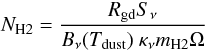 (1)where
Rgd is the gas-to-dust ratio, assumed to be 100,
Sν is the specific flux at
850 μm, 870 μm, or 1.2 mm enclosed within the
IRDC boundary,
Bν(Tdust)
is the Planck function at dust temperature, Tdust,
assumed to be 20 K1. We use the dust model
for intermediate volume densities and thin ice mantles by Ossenkopf & Henning (1994, Table 1, Col. 5), and we
adopt a value for the dust mass absorption
coefficient κ850 μm and
κ875 μm
of 1.85 cm2 g-1 and κ1.2 mm
of 1.0 cm2 g-1. We use the automated clumpfind algorithm
(Williams et al. 1994) to identify
pixels in the smoothed sub-millimeter map which lie above
a 8 × 1020 cm-2,
or AV ~ 0.8 mag, threshold. The resulting
boundary is plotted in the figures in Appendix B.
(1)where
Rgd is the gas-to-dust ratio, assumed to be 100,
Sν is the specific flux at
850 μm, 870 μm, or 1.2 mm enclosed within the
IRDC boundary,
Bν(Tdust)
is the Planck function at dust temperature, Tdust,
assumed to be 20 K1. We use the dust model
for intermediate volume densities and thin ice mantles by Ossenkopf & Henning (1994, Table 1, Col. 5), and we
adopt a value for the dust mass absorption
coefficient κ850 μm and
κ875 μm
of 1.85 cm2 g-1 and κ1.2 mm
of 1.0 cm2 g-1. We use the automated clumpfind algorithm
(Williams et al. 1994) to identify
pixels in the smoothed sub-millimeter map which lie above
a 8 × 1020 cm-2,
or AV ~ 0.8 mag, threshold. The resulting
boundary is plotted in the figures in Appendix B.
For objects not covered by ATLASGAL (see Table 3), we rely on SCUBA archival data at 850 μm and MAMBO 1.2 mm maps to determine boundaries and masses. Unlike the ATLASGAL wide-area maps, the SCUBA and MAMBO data were obtained in targeted fashion, such area of the sub-millimeter map is smaller than the Herschel map size, rendering step 1 of the above boundary definition method unnecessary. We therefore draw a circular boundary to include the significant sub-millimeter emission.
We also estimate the total mass of each cloud assuming optically thin emission and
following the method in Hildebrand
(1983) (2)with
distance, d, considering the flux density,
Sν which is 3-σ above
the average rms in the region. We list the masses in Table 3. We plot the cloud mass as a function of distance in Fig. 4 and as a function of Galactocentric distance in
Fig. 5. Given the uncertainties in dust opacity,
distance, dust temperature, and flux measurements, these mass estimates are reliable to
within a factor of two.
(2)with
distance, d, considering the flux density,
Sν which is 3-σ above
the average rms in the region. We list the masses in Table 3. We plot the cloud mass as a function of distance in Fig. 4 and as a function of Galactocentric distance in
Fig. 5. Given the uncertainties in dust opacity,
distance, dust temperature, and flux measurements, these mass estimates are reliable to
within a factor of two.
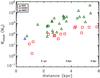 |
Fig. 4 Cloud mass derived from ATLASGAL, SCUBA, or MAMBO continuum maps plotted as a function of distance. Green triangles are IRDCs, red squares are ISOSS sources, and the blue triangle is HMSC 07029. Toward the bottom, the core size we can resolve with our PACS maps is shown as a function of distance. See Sect. 2.3.2 for the relevant assumptions. |
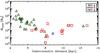 |
Fig. 5 Cloud mass as a function of Galactocentric distance. Green triangles are IRDCs, red squares are ISOSS sources, and the blue triangle is HMSC 07029. |
3. Herschel observations and data reduction
3.1. PACS
We observed 45 sources at 70 μm, 100 μm, and 160 μm with the Photodetector Array Camera and Spectrometer (PACS; Poglitsch et al. 2010). We obtained two perpendicular scan directions to minimize striping in the final combined maps. The scan speed for all observations was 20″ s-1, and a total of 6 repetitions were obtained for each scan direction for the 70 μm, and 160 μm simultaneous observations, while 3 repetitions were obtained for each scan direction for the 100 μm, and 160 μm simultaneous observations and poorly resolved at shorter wavelengths. Map sizes vary according to the target extent and are listed in Table 4. The PACS data for our sources were processed to level 1 using HIPE (Ott 2010). In this step we apply “second level de-glitching” to remove bad data (“glitches”) for a given position in the map. This is done by applying a clipping algorithm (based on the median absolute deviation) to all flux measurements in the data stream that will ultimately contribute to the respective map pixel. For our dataset, we use the “timeordered” option with an “nsigma” value of 25, which removes obvious glitches satisfactorily while keeping the core of stronger point sources intact.
After producing level 1 data, we have generated final level 2 maps using Scanamorphos (Roussel 2012). Because our sources generally fill the scan maps with variable and bright emission, the highpass median–window subtraction method implemented in HIPE for the Level 2 processing produces images which can suffer from variable missing flux levels and stripping at increased levels relative to the Scanamorphos maps. For this reason we choose Scanamorphos as our benchmark level 2 data product. The final level 2 maps were processed using various Scanamorphos v.9 options; we find the “galactic” option to be best suited for our data-set and scientific goals. Additionally, these data were processed including the non-zero-acceleration telescope turn-around data. The resultant maps are presented in the image gallery in Appendix B.
3.2. SPIRE
We obtained maps at 250, 350, and 500 μm using the Spectral and Photometric Imaging Receiver (SPIRE; Griffin et al. 2010). The map dimensions are listed in Table 4. The data were processed until level-1 with HIPE (developer build 5.0, branch 1892, calibration tree 5.1) using the standard photometer script (POF5_pipeline.py, 02.03.2010) provided by the SPIRE ICC team. The level-1 maps were further processed using Scanamorphos (Roussel 2012), version 9 (patched, dated 08.03.2011), which included a de-striping algorithm implemented for maps with fewer than 3 scan legs per scan. We used the “galactic” option and included the non-zero-acceleration telescope turn-around data. The resultant maps are presented in the image gallery in Appendix B.
4. Point source extraction and analysis
4.1. Source extraction and photometry
We first gridded each PACS image to a uniform 1 arcsec per pixel scale. Because of the diffuse, variable background emission in the PACS wavelength regime, the extraction of point sources, in particular for sources deeply embedded in regions of high extinction or with compact background emission components, is not straightforward with a standard algorithm designed for low-background source extraction (e.g. starfinder Diolaiti et al. 2000b). To remedy this, we apply an unsharp-mask filter to each PACS image in order to remove the large-scale emission, i.e. we smooth each image and subtract the smoothed image from the original science frame. We use empirically-determined smoothing filter sizes of 9, 9, and 20 pixels for the 70, 100, and 160 μm bands, respectively. The larger 160 μm filter size is needed because the diffuse emission from the cold material tends to vary on larger scales and this wavelength.
We perform the source extraction with starfinder on the difference image in order to acquire the positions of point sources. These positions are given as a prior for a second iteration of starfinder on the original science frame, on which we perform PSF photometry and extract fluxes on objects which are 5-σ above the median background of the image. We used an empirical PSF of Vesta (Observation Day 160) and rotate to account for the scan direction of a given observation.
Compact source candidates are evaluated internally by starfinder on to which degree they agree with a given instrument PSF. To do this, starfinder computes a correlation coefficient, which is a normalized sum of products of pixel values in the science image and the PSF reference image, taken as a function of spatial offsets between image and PSF. The starfinder algorithm then tries to find the maximum of this coefficient by slightly varying the mentioned spatial offsets. In order to achieve higher accuracy for this estimate, a cubic convolution interpolation method (Park & Schowengerdt 1983) is implemented to compute the correlation coefficient on a sub-pixel level. The explicit form of the correlation coefficient is given in Sect. 3.4 of Diolaiti et al. (2000a), and was itself taken from the book of Gonzalez & Woods (1992). Since the coefficient is a normalized quantity, a perfect agreement between a source in the science frame and the PSF would result in a correlation coefficient of 1.0. As mentioned in Diolaiti et al. (2000a), a correlation coefficient between 0.7 and 0.8 is still acceptable in case of noisier data to consider a found source as an unresolved source resembling the PSF. We tested a range of required correlation coefficient values and determined by-eye that a value of 0.79 was most suitable.
Where available, we use 24 μm images from the Spitzer/MIPS archive, mainly from the MIPSGAL survey (Carey et al. 2009). We indicate which of our targets were covered by MIPSGAL or other MIPS 24 μm observations in Table 4. We extract the point source flux from the MIPS 24 μm image using the tinytim PSF. We then match all catalogs using a world coordinate system-based algorithm (see Gutermuth et al. 2008) with a position-matching tolerance of 11′′ (the FWHM of the PACS 160 μm PSF), and we report the position (from the 100 μm source position) and flux densities of all sources detected in at least the three PACS bands in Table C.1. The positions of the point sources are marked on each panel in the image gallery figures (Appendix B). The uncertainties in extracted flux densities are of order 15, 20, and 20% for PACS 70, 100, and 160 μm, respectively, and 15% for the MIPS 24 μm flux densities.
We cross correlate our PACS point source catalog with the IRAS and MSX point source catalogs and note matches in Table C.1. In cases where the MIPS 24 μm image is saturated, we list the IRAS 25 μm or MSX 21 μm flux density. We note that the IRAS and MSX fluxes are integrated over much larger apertures than MIPS and PACS, so in some cases there are multiple source resolved with Herschel or Spitzer which appeared as a single source in IRAS or MSX. Some sources in Table C.1 have the same associated IRAS or MSX source.
In all, we extract 496 point sources which have counterparts at all PACS wavelengths. Upon by-eye inspection, we identified 51 point sources which appear point-like in the PACS bands but did not meet our criteria for significance and/or PSF-correlation coefficient. On the other hand, 152 of the 496 sources were deemed “unlikely” to be identified by the human eye. In summary, 70% of the reported detections are reliable when checked by eye, and an additional 10% could be missing from the sample. These figures do not include the differing effects of distance on our ability to resolve substructure within the psf; such considerations will be addressed in forthcoming work on individual objects which can be supplemented when high-resolution data become available (e.g. Beuther & Henning 2009).
4.2. Spectral energy distribution fitting
We fit a single temperature modified Planck function to the spectral energy distribution (SED) comprised of the three PACS flux densities (Sν) at 70, 100, 160 μm at the position of each extracted point source. At these wavelengths, we assume the dust is optically thin. We exclude the SPIRE data in order to preserve the high angular resolution scales probed with just the PACS data. Furthermore, for the vast majority of point sources, no clear counterpart is possible to extract from SPIRE maps due to increasing beam dilution. We also exclude the 24 μm data point in our fitting. Beuther et al. (2010) have shown that a second blackbody contribution, with a higher temperature and lower mass, is typically needed to account for the 24 μm emission. This second blackbody represents the relatively small fraction of warm dust which lies near the central protostar, presumably because this material has been heated by the protostar itself. We revisit this interpreation in Sect. 5.
The automated fitting is performed with simulated annealing (Kirkpatrick et al. 1983). The model takes into account the
frequency-dependent, optically thin dust opacity,
κν, using the model computed by Ossenkopf & Henning (1994), assuming a density
of 106 cm-3 and thin ice mantles on the grains. The SED comprised of
the extracted flux densities are fit iteratively with the following function:
 (3)where
Bν is the Planck function at a
temperature, Tdust, Rgd is the
gas-to-dust ratio (assumed to be 100), d is the distance to the source,
and M is the gas mass fit for a given object. We stress that
Tdust represents a single, average temperature of the
unresolved point source, and here we do not attempt to model the temperature gradient on
smaller scales.
(3)where
Bν is the Planck function at a
temperature, Tdust, Rgd is the
gas-to-dust ratio (assumed to be 100), d is the distance to the source,
and M is the gas mass fit for a given object. We stress that
Tdust represents a single, average temperature of the
unresolved point source, and here we do not attempt to model the temperature gradient on
smaller scales.
4.3. Sensitvity considerations
The PACS photometer has in general shown a good performance regarding point source detection sensitivities. In the scan map release note2 5-σ detection limits of around 5, 5, and 11 mJy are mentioned for the 70, 100, and 160 μm filter, respectively. This performance has been achieved on mini-maps (having a similar number of scan repetitions as our science maps, but better coverage in the central part of such a map). However, we cannot expect identical detection thresholds for our science maps. First, the benchmark results have been obtained in observations of field stars without high extended background emission. Furthermore, these mini-maps have been processed by utilizing the standard approach for drift and 1/f noise removal: an aggressive high-pass filtering of the data time lines with small median windows, which robustly pushes the noise in the map to very low levels. Such an approach is not possible for our science maps since it would severely corrupt the extended emission present in our maps, and would at the same time affect the point source fluxes. Instead of high-pass filtering we use the Scanamorphos program (see Sect. 3.1) as a well-balanced compromise for retaining both the correct point source fluxes and the extended emission, at the cost of slightly higher noise levels. Because the objects in our sample exist in a wide variety of environments, and the foreground and background emission varies not only from region to region but also within a given map, the overall point source sensitivity is difficult to quantify. In general, the minimum fluxes we detect are 0.03 Jy at 70 μm, 0.03−0.1 Jy at 100 μm, and 0.1−0.3 Jy at 160 μm. Naturally, the sensitivity worsens in regions of bright, diffuse emission (e.g. IRDC 18102 and 18454).
5. Spectral energy distributions
In Table C.1, we present a catalog of all point sources found in the 45 targets, requiring detections in all three PACS bands, and report their positions and flux densities. We enforce strict extraction and matching criteria (see Sect. 4) in order to compile the most homogeneous, flux-limited catalog possible with these data. There are a total of 496 cores which fit this description. Where available (see Table 4), we include the MIPS 24 μm flux density when a counterpart is present. For bright sources, the MIPS detector is often saturated, in which case we report an IRAS 25 μm flux density or MSX 21 μm flux density, when one was available. We note that in such cases, the IRAS and MSX fluxes are measured over much larger beam areas, thus the reported flux density will certainly be an overestimate of that due to the Herschel point source.
The clouds in our sample span a range of distances from 0.6 to 5.9 kpc (see Fig. 2). One consequence of the large range of distances is that the definition of a “point source” corresponds to different physical scales throughout the sample. For example, in the nearest IRDC at 0.63 kpc, the 11.4′′ angular resolution of the 160 μm band corresponds to 7200 AU, or 0.03 pc, which resolves what is considered a typical core scale (Bergin & Tafalla 2007). On the other hand, a point source in the most distant IRDC at 5.9 kpc corresponds to a physical scale almost ten times larger, which is closer to the “clump” scale, an object which could be comprised of many “cores”. As a result, we are more sensitive to the low-mass, low-luminosity population of cores in nearer IRDCs than the more distant ones. Therefore, throughout our analysis, we distinguish between point sources within “near” and “far,” using 4 kpc as the defining distance. A point source in the “near” category has a characteristic physical scale of 0.1 to 0.2 pc, and a “far” point source is between 0.2 and 0.3 pc. The range of physical sizes to which our point sources correspond is illustrated in Fig. 4. Because most clouds reside in the near regime, we will, for simplicity throughout the remainder of the paper, refer to the point sources as “cores”, the physical interpretation of these objects. When relevant for comparing sample properties, we normalize flux to a distance of 4 kpc so the properties of the entire sample can be fairly compared.
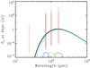 |
Fig. 6 Example SED for a core with the median properties of the “near” sample: M = 2 M⊙ and T = 20 K. The solid black curve depicts the SED assuming optically thin emission over the full spectrum. The cyan dashed curve shows an SED with the same parameters, but without an assumption of optically thin emission. The blue, green, and red dash-dotted curves show the filter response function (× 10-3) for the 70 μm, 100 μm, and 160 μm bands, respectively. The full range of fluxes at each wavelength for 24 μm-bright (red dotted line) and 24 μm-dark (gray dotted line) are shown. All flux densities have been normalized to the fiducial 4 kpc distance. |
We construct SEDs for each source having detections in at least the three PACS bands. In Table C.1, we list the flux densities at 70, 100 and 160 μm, as well as the 24 μm flux density when available3. Figure 6 shows the full range of flux densities, normalized to 4 kpc distance as well as the fit (from Eq. (3)) SED of a core with the median properties of the sample. The solid curve shows the fit assuming optically-thin emission, and the dashed curve shows a Planck function with the same physical properties but without the optically-thin assumption (but assuming NH2 ~ 1023 cm-2). The total luminosity differs by only ~10%.
The SEDs peak in the range between 130 and 190 μm, and the median peak flux density (of the 4 kpc distance-normalized SED) is about 1 Jy at 160 μm. Figure 7 shows example SEDs for individual objects selected to show the full range in luminosities of the sample with the best fit modified blackbody with (solid line) and without (dashed line) the optically thin assumption.
The 24 μm flux density typically can not be accounted for in the single component, single temperature fit to the PACS flux densities, but instead requires a second “warm” component to be added. We opt to exclude the value of the 24 μm data point in the analysis that follows for several reasons. First, shortward of 70 μm, the optically thin assumption is less reliable, rendering the 24 μm flux density a poor constraint of the warm component to extract meaningful physical information from a second component. Secondly, as the point sources are unresolved, probing scales between 0.05 to 0.3 pc, the enclosed volume is (by mass) dominated by the passively-heated outer core (van Dishoeck et al. 2011). A complete treatment of the core radiative transfer is beyond the scope of this paper. Recent work by Stamatellos et al. (2010) and Pavlyuchenkov et al. (2012) demonstrate the need for observations such as those presented here to constrain the flux on all scales in order to refine models.
Each SED fit using Eq. (3) has a best-fit temperature and mass, and the integrated area under the function gives the total luminosity, all of which are reported in Table C.1. As we are probing on scales of 0.05 to 0.3 pc (“cores”), these quantities represent the average values over the enclosed region. While we do not include the value of the flux density at 24 μm, we instead at times indicate whether a source is “24 μm-bright” or “24 μm-dark”, meaning that there is or is not (respectively) a counterpart at a given position in the 24 μm image (or IRAS/25 μm or MSX/21 μm). We return to the significance of the 24 μm detections later in the Discussion.
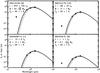 |
Fig. 7 Example SEDs of objects at a range of luminosities: 873 L⊙ (top left), 98 L⊙ (top right), 10 L⊙ (bottom left), and 1 L⊙ (bottom right) cores, all normalized to 4 kpc distance. The cloud name and core ID number of the object are given in each panel, along with the mass and temperature, and all associated uncertainties. The dashed line in each panel represents the SED without the optically thin assumption. |
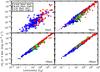 |
Fig. 8 Flux at 24 μm (upper-left), 70 μm (upper-right), 100 μm (lower-left), and 160 μm (lower-right), normalized to 4 kpc distance, as a function of luminosity from SED fits. The black crosses and blue diamonds represent the 24 μm-dark and -bright (respectively) cores nearer than 4 kpc. The green squares and red x’s represent the 24 μm-dark and -bright (respectively) cores further than 4 kpc. The magenta dashed line in the two upper panels represents the relationship shown in Dunham et al. (2008) for embedded protostars from the Spitzer c2d survey. |
5.1. The source of emission at PACS wavelengths
In Fig. 8 we plot the relation between the flux (νSν) at each band and the corresponding core luminosity. There is a direct correlation at each wavelength which tightens at longer wavelengths. Dunham et al. (2006, 2008) find that for low-mass protostars, the 70 μm flux (from Spitzer in their case) is key to directly probing the protostellar luminosity while not being heavily influenced by external heating or the disk geometry, which more strongly impacts the 24 μm emission. The upper-right panel of Fig. 8 shows this correlation extends to the higher-luminosity cores we find in IRDCs. We also show in Fig. 8 that the 100 μm, and moreso the 160 μm, fluxes are excellent proxies for the core luminosities. But what is the main contributor to the 100 and 160 μm flux in IRDC cores: the protostellar luminosity or the external heating?
Dunham et al. (2006, 2008) argue that, for low-mass protostars, at wavelengths of 100 μm and longer, the external radiation field becomes important, however because cores in IRDCs are generally more massive and more luminous, and by deduction home to more massive and luminous protostars, the balance between internal heating from a protostar and external heating from the interstellar radiation field (ISRF) and/or local sources may be different. Further complicating the picture is that the dense environments of IRDCs, the cores we detect are embedded in high column density material (AV ~ 2−20 Kainulainen et al. 2011), which may serve shield the core material from significant heating from external sources. While Pavlyuchenkov et al. (2012) have shown that the stochastic heating caused by external UV field contributes insignificantly to the SED of IRDC cores longward of 100 μm, further radiative transfer experiments are needed to quantify the impact of external radiation on the core heating and resultant SED of more massive cores at PACS wavelengths.
As a simple test of this question, we perform one-dimensional radiative transfer calculations using the TRANSPHERE-1D4 (vers. 3, C. Dullemond), a spherically-symmetric version of the code presented in Dullemond et al. (2002), which is specially suited for high optical depth scenarios like our massive cores. We assume the core has a density (ρ) profile, ρ(r) ∝ r-2, where r is the radius. The average central density was 106−7 cm-3 over the integrated radius range between 200 AU and 0.1 pc, which are similar to the values used in recent radiative transfer calculations of IRDC cores (Stamatellos et al. 2010; Wilcock et al. 2011). At the assumed distance, 4 kpc, the core would be 10′′ in diameter, which would be unresolved in our PACS 160 μm observations.
We assume a hybrid ISRF with the Black (1994) model for λ > 0.36 μm and Draine (1978) for λ < 0.36 μm, as was done in Evans et al. (2001), and we implement dust opacities from Ossenkopf & Henning (1994) for λ > 1 μm and Mathis et al. (1983) for λ < 1 μm. We test cases for a 10 M⊙ core, both with and without an internal protostar. For the protostellar case, we assumed a protostellar temperature of 8000 K, mass of 1 M⊙, and radius of 5.3 R⊙, motivated by models of massive protostars by Hosokawa & Omukai (2009) taking into account both the protostar and accretion for a Ltot ~ 2 L⊙. Our simplified test assumes a single central source, but indeed most massive stars form in systems. Assuming that the sources are tightly clustered in a heavily embedded central region, the total, reprocessed emission coming out of the optically thick central core region will be most relevant for these calculations.
In Fig. 9, we show the resultant SED for a 10 M⊙ core with and without an internal protostar, and with varying levels of external radiation field, from no ISRF, a Black & Draine (B+D) ISRF, and a ten times amplified B+D ISRF. The SED is normalized to a distance of 4 kpc. In the protostellar case, indeed we only begin to see a difference due to the ISRF at wavelengths longward of 100 μm, and only marginally there. The bigger difference is seen when the protostellar SEDs are compared to the starless cases, where the only heating source is external. As the ISRF level is increased, the SED is significantly enhanced at wavelengths longer than 60 μm. With enough enhancement of the ISRF, an externally headed starless core could mimic the FIR SED of a protostellar core. However, we note that even in the extreme case of a ten times amplified ISRF, no appreciable 24 μm flux is produced in the starless case. In future work, we shall explore the parameter space of core environments and the temperature structure.
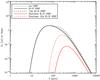 |
Fig. 9 Results of TRANSPHERE-1D radiative transfer calculations for a 10 M⊙ core. The black lines represent the protostellar cases with varying levels of the B+D ISRF (see text). The dotted line has no ISRF, the solid line shows a “standard” B+D ISRF, and the dashed line shows the case for a ten times (uniformly) amplified B+D ISRF. The red lines represent the case for starless cores, and are for the same ISRF cases. |
5.2. 24 μm emission
Figure 9 shows that a 10 M⊙ core with a protostar would be detectable at 24 μm, but as the core mass increases, the cores become more optically thick, thus the energy radiated at short wavelengths is reprocessed and re-emitted at the longer wavelengths. Here we emphasize that while such a trend is not surprising for the spherical symmetric cases. At these wavelengths the core geometry likely plays a strong role, so our simple 1D model breaks down. The central region is optically thick at 24 μm, thus other effects are needed to account for the 24 μm flux.
There are various ways of accounting for the emission seen at 24 μm. We have discussed emission from externally, isotropically heated outer core regions and emission from inner core regions. The emission from the inner core region generally would be reabsorbed by the outer core, but the inner core can be exposed by outflow activity when the jet/outflow alignment allows for it or the inhomogeneous distribution of clumpy material around the warm inner core (Indebetouw et al. 2005). A core which is heated (anisotropically) by the radiation from a near neighbor can bring about excess emission as well, but we show in Fig. 10 that even in the case of the most enhanced ISRF, the amplification of flux does not appear at short wavelengths. Further studies will be needed to examine for single cores if nearby stellar sources can contribute to the heating of the core and thus to the flux at 24 μm. But given the numerous detection of 24 micron excess, it seems unlikely that all of them have stars close enough to impact the SED and which can illuminate the core unattenuated.
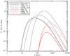 |
Fig. 10 Results of TRANSPHERE-1D radiative transfer calculations for a 10, 100, 1000 M⊙ protostellar (PS) and starless (SL) cores with the standard B+D hybrid model for the ISRF. The black lines represent the protostellar cases for 10 M⊙ (solid line), 100 M⊙ (dashed line), and 1000 M⊙ (dashed-dotted line). The red lines represent the same masses but without a central protostar. |
Substantial 24 μm flux would also be expected in the case when the entire core has been heated by the central source enough that the optical depth at 24 μm becomes low enough that this emission can leave the core un-extincted. Because our observed SEDs can be fitted best with a single modified blackbody spectrum with low temperatures, we conclude that the 24 μm emission visible in some cases is not due to a global warming of the core but is rather emission from heated inner regions exposed by outflow activity.
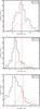 |
Fig. 11 Distribution of point source properties within “near” (black histogram) and “far” (red dotted histogram) IRDCs. The top panel shows the core temperature distribution; the center panel shows the core luminosity distribution, and the bottom panel shows the core mass distribution. The median values for the near (black) and far (red) distributions are plotted with the vertical dashed lines. |
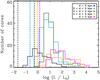 |
Fig. 12 Histograms of core luminosities in distance bins d < 2 kpc (black), 2 < d < 3 kpc (blue), 3 < d < 4 kpc (green), 4 < d < 5 kpc (orange), and d > 5 kpc (magenta). The vertical dashed lines represent the luminosity sensitivity for each corresponding color distance bin. |
6. Sample property distributions
We plot the distribution of fit parameters for the full set of 496 cores in our sample in Fig. 11. We distinguish between “near” and “far” sources using 4 kpc as the dividing distance. At 4 kpc and nearer, we probe scales of 0.2 pc and below. In total, there are 364 cores within near IRDCs and 132 cores within far IRDCs. We note that there are two factors which will reduce the number of cores detected in “far” IRDCs: (1) low-mass cores will fall below our detection limit, and (2) due to coarser resolution of physical scales, cores which are separated by less than 0.2−0.3 pc will not be resolved.
The core temperatures have a 18 K spread, and both the near and far cores have median values of 20 K. The median mass for near cores is 2 M⊙, and the luminosity distribution is strongly peaked around the median 10 L⊙. For cores in far IRDCs, the median of the distribution are 14 M⊙ and 109 L⊙ for the mass and luminosity, respectively, however our sensitivity to the low mass and low luminosity populations in far objects is limited. We show in Fig. 12 the luminosity distribution broken down into more refined distance bins. From Fig. 8, a core at our flux density limit at 160 μm (0.1 Jy) corresponds to a 1 L⊙ core at 4 kpc. At nearer distances, we can detect sources down to 0.25 L⊙ at 2 kpc, and our sensitivity worsens to 2.3 L⊙ at 6 kpc. As was discussed in Henning et al. (2010), assuming flux uncertainties for the 70, 100, and 160 μm bands of 15%, 20%, and 20%, respectively, the uncertainties to the fits are 4% in the temperature, 20% in the luminosity, and 50% in the mass. These uncertainties do not include the effects of optical depth, which, for example, can lead to underestimates of the mass.
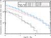 |
Fig. 13 The cumulative mass function of cores more massive than 1 M⊙. The total distribution of all cores is shown in blue solid line; the distribution of 24 μm-bright cores is shown in the red dash-dotted line; the distribution of 24 μm-dark cores is shown in black dashed line. A simple linear regression was fit to each distribution, taking the functional form N(>M) ∝ Mα. For reference, on this scale, a Salpeter slope is α = 1.35. |
6.1. Core mass function
In Fig. 13 we show the cumulative mass function of cores more massive than 1 M⊙, including the total distribution, then the distributions split in terms of the 24 μm counterpart status of a given core. We fit the distributions with the function N(>M) ∝ M−α. We find that the slope of the full distribution is α ~ 0.67 ± 0.26, while the 24 μm-bright cores have a slightly shallower distribution (α ~ 0.57 ± 0.26) and the 24 μm-dark cores have a steeper distribution (α ~ 0.88 ± 0.47).
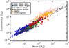 |
Fig. 14 Core luminosity versus core mass. We make four categories of sources: “near” sources, which are closer than 4 kpc, with either a 24 μm counterpart (“bright”) or no 24 μm counterpart (“dark”), and “far” sources with the same bright/dark distinction. For comparison, we plot in orange triangles the Beuther et al. (2002b, 2005a) sample of high-mass protostellar objects (HMPOs) and the Hunter et al. (2000) sample of ultra-compact HII regions in pink squares. With the black dashed line, we plot a line of constant accretion luminosity, Lacc = GṀMstar/Rstar, of 10-5 M⊙ yr-1, assuming Mstar = 0.1 Mcore and Rstar = 5 R⊙, and the range indicated by the grey dashed lines on either side show ± 1 dex variation. See Sect. 6.2 for details. |
Figure 13 immediately confirms what has been shown in the past in other high-mass regions (e.g. Motte et al. 2007) is also true in IRDCs: very massive cores (with M > 100 M⊙) are rare, and those that we do find are quite likely to be mid-infrared bright. While the sampling is not uniform, thus the errors on the fit are quite large, we find general agreement of the clump mass functions massive regions in M17 from Stutzki & Guesten (1990, α ~ 0.72, and IRDCs in Ragan et al. (2009, α ~ 0.76, though it shallower than the log-normal function to the IRDC fragments in Peretto & Fuller (2010) which follows a α ~ 2 slope in this mass regime.
6.2. Mass-luminosity relationship
At the earliest embedded stages, accretion luminosity is believed to dominate the total luminosity of a core, and with time, the contribution of the protostellar luminosity grows (Hosokawa & Omukai 2009). In Fig. 14, we show the relation between core mass and total luminosity of the population of cores presented in this work. For comparison, we also plot the positions more evolved objects: ultra-compact HII (UCHII) regions from the Hunter et al. (2000) sample and high-mass protostellar objects (HMPOs Beuther et al. 2002b, 2005a), believed to be the precursor to UCHII regions. HMPOs and UCHII regions occupy the highest mass and luminosity part of the diagram, but also overlap with the most luminous objects in our sample. We note that the masses and luminosities for the UCHII regions and HMPOs were measured over larger apertures than the PACS cores, thus their masses and luminosities are integrated over a larger region that includes both the protostar and its surroundings, potentially inflating the estimates of the mass and luminosity of the driving protostar.
Based on empirical accretion models by Saraceno et al.
(1996) and Molinari et al. (2008), objects
on this diagram move from the lower right to the upper left of this plot as they evolve.
In this picture, our Herschel sources appear less evolved than HMPOs and
UCHII regions, though the distinction is marginal. In Fig. 14, we show a line of constant accretion rate,
10 yr-1,
and show the associated accretion luminosity,
Lacc = GṀMstar/Rstar,
where we assume the radius of the accreting protostar, Rstar,
is 5 R⊙ and the accreting protostellar mass,
Mstar, is 0.1 times a given core mass (the quantity plotted
on the x-axis). We show a spread of an order of magnitude in either direction, which can
arise from higher accretion rates or variations in the assumed protostellar mass or
radius. In addition, the luminosity of more evolved objects (such as HMPOs and UCHII
regions) will include a larger contribution from the protostar than the youngest objects,
which is not included in our simple calculation. Detailed models of non-spherical
accretion are needed (e.g. Krumholz et al. 2009;
Kuiper et al. 2010) to disentangle the growth of
the most massive protostars.
yr-1,
and show the associated accretion luminosity,
Lacc = GṀMstar/Rstar,
where we assume the radius of the accreting protostar, Rstar,
is 5 R⊙ and the accreting protostellar mass,
Mstar, is 0.1 times a given core mass (the quantity plotted
on the x-axis). We show a spread of an order of magnitude in either direction, which can
arise from higher accretion rates or variations in the assumed protostellar mass or
radius. In addition, the luminosity of more evolved objects (such as HMPOs and UCHII
regions) will include a larger contribution from the protostar than the youngest objects,
which is not included in our simple calculation. Detailed models of non-spherical
accretion are needed (e.g. Krumholz et al. 2009;
Kuiper et al. 2010) to disentangle the growth of
the most massive protostars.
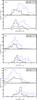 |
Fig. 15 Distribution of point source properties within “near” and “far” IRDCs (top and bottom of each panel, respectively). The top panel shows the temperature distribution; the center panel shows the luminosity distribution, and the bottom panel shows the mass distribution. The black histogram shows objects which have no 24 μm counterpart, and the blue dashed histograms show the distribution of objects with a 24 μm counterpart. |
6.3. Evolutionary stage of cores
6.3.1. 24 μm counterparts
Out of the 496 cores in our sample, 422 have complementary 24 μm data available. Of those 422 cores, 278 (66%) have counterparts at 24 μm. The appearance of a 24 μm counterpart5 has, to-date, been interpreted as a signpost for a local heating source (Beuther & Steinacker 2007; Beuther et al. 2010), but the mechanism by which 24 μm escapes had not been determined. As we discussed above, unless an outflow of some kind clears away some of the outer dense core material, the high optical depth at 24 μm would prevent us from detecting a counterpart. In the following we explore the connection between the outer core properties, as probed by our PACS observations, and the presence of a 24 μm counterpart. We note that the non-detection of a 24 μm counterpart does not necessarily mean that there is no protostar present because the geometry may be such that high optical depth blocks the emission from the heated cavity. Therefore, some overlap between the “dark” and “bright” populations can be expected.
In Fig. 15, we examine the property distributions taking into account whether or not the core has a counterpart at MIPS 24 μm. The median core temperature for near (far) dark cores is 18.6 K (19.5 K) and 21.1 K (21.9 K) for bright cores. In addition, MIPS-bright cores tend to be more luminous, with the median value of 13 L⊙ (173 L⊙) for near (far) MIPS-bright cores compared to 9 L⊙ (56 L⊙) for near (far) MIPS-dark cores. The same trend holds for the masses, where near (far) MIPS-bright cores have a median mass of 3 M⊙ (16 M⊙) compared to the 2 M⊙ (13 M⊙) median for MIPS-dark cores.
Figure 16 shows a PACS color-color diagram for
each core detected in the three PACS bands. The color based on wavelengths
A and B is calculated as follows:
![Mathematical equation: \begin{equation} [A] - [B] = -2.5~\log \left( \frac{\nu_{A}~S_{A}}{\nu_{B}~S_{B}} \right) \end{equation}](/articles/aa/full_html/2012/11/aa19232-12/aa19232-12-eq80.png) (4)we
differentiate between cores with and without MIPS 24 μm counterparts in
Fig. 16. In both colors, [70] – [100] and
[100] – [160], 24 μm-dark cores are redder (larger numbers in color
space) than 24 μm-bright cores, though the two populations occupy the
same ranges in color space independently of distance. In Fig. 16 we also plot the color distribution for an additional population
of 312 candidate cores from our EPoS sample which appear only at 100 and
160 μm. Since these cores only have two data points in their SEDs, we
can not model their properties to the extent we have for cores detected in all three
PACS bands. However, we have computed their [100] – [160] color, and we find that the
colors are consistent with a yet colder (on average) population of cores than
the 24 μm and 70 μm-bright cores.
(4)we
differentiate between cores with and without MIPS 24 μm counterparts in
Fig. 16. In both colors, [70] – [100] and
[100] – [160], 24 μm-dark cores are redder (larger numbers in color
space) than 24 μm-bright cores, though the two populations occupy the
same ranges in color space independently of distance. In Fig. 16 we also plot the color distribution for an additional population
of 312 candidate cores from our EPoS sample which appear only at 100 and
160 μm. Since these cores only have two data points in their SEDs, we
can not model their properties to the extent we have for cores detected in all three
PACS bands. However, we have computed their [100] – [160] color, and we find that the
colors are consistent with a yet colder (on average) population of cores than
the 24 μm and 70 μm-bright cores.
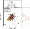 |
Fig. 16 PACS color–color diagram showing the 24 μm-dark cores (red) and 24 μm-bright cores (black). All sources with high luminosities (L > 103 L⊙) are shown in green. The typical error is plotted in the lower-left corner. The right panel shows the distribution of [70] – [100] colors, and the upper panel shows the distribution of [100] – [160] colors for the 24 μm-bright cores (red), 24 μm-dark cores (black), and (in blue) cores for which no counterpart at 70 μm was detected. |
The uniformity of PACS colors for all cores confirms the idea that in the far-infrared, the emission is dominated by the cold core “envelope”. Whether or not a core is detected at 24 μm may be a reflection of the more advanced evolutionary stage of the 24 μm-bright cores: one where the evolving protostar launches an outflow, exposing the warm inner regions. cores dark at 24 μm can also be protostellar, but aligned such optically thick material in the core obscures the 24 μm emission from our view, or they may be pre-stellar/starless with heating from an external sources (see Fig. 9), or they are more deeply embedded and therefore obscured from view.
The presence of a 24 μm counterpart coincides with the warmer, more luminous, and more massive cores of the population, though the effect appears small. We see in Fig. 11 that while the distance to a source affects our ability to detect low-mass and low-luminosity cores, we see no effective difference in the temperature range as a function of distance. If the existence of a 24 μm counterpart is indeed the consequence of the later evolutionary state of the core, we expect that in more evolved cores, the outer core gas would have experienced the heating from the internal source, an effect which is also seen for the dense gas in IRDCs reported in Ragan et al. (2011). Since we do not resolve the cores, we derive only the line-of-sight average core temperature, but the 1.5 to 2 K increase in temperature in 24 μm-bright cores is similar to the gas measurements. To fully characterize the evolutionary differences in detail likely requires the inclusion of the near to mid-infrared data points with a full treatment of the optical depth effects. Such an undertaking is beyond the scope of this paper but will be addressed in forthcoming work.
Our ability to detect 24 μm counterparts worsens with increasing distance, which in turn will cause our estimates of the frequency of 24 μm counterparts to be too low. Figure 17 shows the fraction of cores which are 24 μm-bright and 24 μm-dark as a function of distance. We calculate this fraction only for the targets covered with MIPS observations. Because we become less sensitive to faint sources with increasing distance, we expect this to be an observational bias.
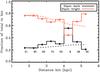 |
Fig. 17 In solid lines, we plot the fraction of cores which have a 24 μm counterpart (red solid line, triangles) and those without 24 μm counterparts (black solid line, diamonds). We plot this fraction only for targets which have available MIPS 24 μm data, as indicated in Table 4. The dashed line represents how the fraction of 24 μm bright/dark cores would change if the cores in the nearest bin were placed in the progressively larger distance bins. The uptick at large distances of 24 μm-bright fraction is due to the particularly active IRDCs at these distances. |
The dashed line in Fig. 17 shows how we would expect the fraction of 24 μm-bright to dark sources would fall off with increasing distance assuming distance was the only factor at play in hindering the detectability of counterparts. To make this estimate, we assume that the distribution of 24 μm fluxes and also the fraction of 24 μm-bright cores is representative of the sample. We then project this subset of cores to each distance bin and compute the fraction that would fall below the flux detection limit at that distance. This does not appear as a straight line because the fluxes are not smoothly distributed within the nearest bin. We confirm that the general trend can be explained as a observational bias. The fact that we detect a rise in the detection frequency of counterparts at large distances is due to the very active regions (e.g. IRDC18454 near W43) where the we find a large fraction of 24 μm-bright sources.
We cross-correlate our catalog with the young stellar object catalog by Robitaille et al. (2008) for the 27 IRDCs which are part of the GLIMPSE I and II datasets. Within a matching radius of 10′′, there are 40 objects in our sample that appear in the Robitaille et al. (2008) catalog, all but six of which are bonafide YSOs and not AGB contaminants (Robitaille, priv. comm.). All of the YSOs have 24 μm counterparts and tend to have temperatures above the sample median (20 K).
6.3.2. Other signposts of star formation
Extended green objects (EGO, Cyganowski et al. 2008; Chambers et al. 2009) are areas of enhanced diffuse emission in the “green” band (4.5 μm) of the Spitzer/IRAC camera. This is thought to be a result of shocked-H2 emission line which falls into that band (De Buizer & Vacca 2010) or due to scattered continuum emission (Takami et al. 2012). In the catalog of Cyganowski et al. (2008), five EGOs (in four IRDCs) are found within 10′′ of a core in our catalog, and in the Chambers et al. (2009) catalog, six “green fuzzy” (G.F.) regions in three IRDCs match with core positions. The matching cores and their EGO classification are given in Table 1. Ten of the eleven matching cores with EGO activity have a 24 μm counterpart, and their temperature range from 13 to 24 K.
IRDC cores associations with EGOs.
SiO emission is a well-known tracer of shocked gas, widely used to search for outflows originating from young stars. The targets in our sample have not been uniformly surveyed for SiO emission, therefore we can not say with statistical certainty whether SiO is associated with just 24 μm-bright cores or not. Nonetheless, we compare our core catalog with the Beuther & Sridharan (2007) survey of SiO(2−1) emission overlaps with 12 of the IRDCs in the sample (see Table 3). Further follow-up observations of SiO(2−1) with the IRAM 30-m telescope have been performed on 8 additional IRDCs in a recent survey by Vasyunina et al. (2011) and (Linz, in prep.). These single point observations do not have sufficient resolution (28′′) to resolve the outflow structure, but we find that in 90% of the cases, the nearest core to the peak position of the SiO emission coincides with a core with a 24 μm counterpart.
Cores which are bright at 24 μm appear to be (1) warmer, (2) consistent with YSO colors when detectable at mid-infrared bands, and (3) often in close spatial association with molecular outflow tracers. Unfortunately, a full sampling of all cores is not available or falls outside of the selection criteria of these supplementary surveys, so we can not quantify these trends. In any case, the catalog presented in this work provides an expanded range of conditions or evolutionary stages which can be further observationally explored.
Most extreme 24 μm-dark cores.
7. Discussion
7.1. The nature of the cores
We present a core (size ~0.05 to 0.3 pc) population for which we model the temperature, mass, and luminosity of the cold, outer shell of the core where the bulk of the mass resides. Despite not including the 24 μm flux density in our SED fits, the shells surrounding 24 μm-bright cores appear to be warmer than 24 μm-dark cores. In addition, previous surveys of YSOs and outflows show that these independent indicators of embedded star formation tend to be coincident with 24 μm-bright cores. While supplemental survey data are not uniformly available for the full EPoS sample, we are unable to show correlations with statistical significance. However, at face value, the warmer, 24 μm-bright cores appear to be associated with more star formation activity than the colder, 24 μm-dark cores, and hence the 24 μm-bright cores could be in a more advanced evolutionary stage.
We find a tight relation between the far-infrared flux and the core luminosity (see Fig. 8) which we would not expect if the flux was dominated by a stochastic external radiation field at PACS wavelengths. Still, at 24 μm we find the largest scatter in the relationship where the influence of the external radiation field is stronger (Pavlyuchenkov et al. 2012). Wilcock et al. (2011) show that on larger scales (0.4 to 1 pc) temperature gradients due to enhanced interstellar radiation fields are important in modeling the SEDs of IRDC clumps. On the core scale, however, the impact of embedded sources will be greater and the influence of the external radiation field (at PACS wavelengths) will be more effectively shielded by the high column density material in which the cores are embedded.
The fits to the core temperatures are strongly peaked between 15 and 25 K. Typical gas temperatures in IRDCs of the clouds on larger scales have been found to be between 8 to 17 K (e.g. Sridharan et al. 2005; Pillai et al. 2006a; Ragan et al. 2011), based on measurements of the NH3(1, 1) and (2, 2) inversion transition lines. A similar range is found in the dust temperatures (e.g. Peretto et al. 2010). Furthermore, high resolution measurements of temperature in IRDCs (Devine et al. 2011; Ragan et al. 2011) show small scale enhancements of gas temperature near regions of active star formation, i.e. when 24 μm emission is present. Assuming the gas and dust are thermally coupled, which should be the case for the density regime of IRDCs (Goldsmith 2001), the presence of protostars and gradual heating of the surroundings has already been observationally connected.
Every line of evidence presented above suggests that at least cores with a 24 μm counterpart are protostellar. But what about the newly uncovered population of cores found only at 70 μm and longward? Such sources comprise 34% of our core catalog. Apart from the higher median temperature associated with 24 μm-bright sources, there is little difference between the masses and luminosities of 24 μm bright and dark sources. Are they objects at an earlier evolutionary stage, or are they at the same stage but we are somehow biased against detecting 24 μm counterparts for some sources?
As we discussed above, the detection of 24 μm counterpart is possible if our line of sight permits us to peer into a cavity formed by outflowing material to view emission from warm dust near the central source. Cores dark at 24 μm can still contain protostars, but by chance our line of sight does not include the warm dust emission. Alternatively, they may be starless with some degree of external heating by the ISRF or a neighboring source. The 24 μm data alone can not tell us which is the case for a given dark source. (Arce et al. 2007) show that massive protostars can carve a large variety of cavities in their host core, so it is difficult to rule out either scenario based on the present statistics. Here, we instead turn the correlations seen in the cold outer core to inform our understanding of the 24 μm-dark cores which comprise 34% of our sample.
The warmer outer-core temperatures associated with 24 μm-bright cores supports the interpretation that they are more evolved than 24 μm-dark cores. Because of the observational issues mentioned above, there is unavoidable overlap such that protostellar cores are not detected at 24 μm. The idea that 24 μm-bright cores are in a more advance evolutionary stage than 24 μm-dark has been suggested before in Chambers et al. (2009) when considering the correlation between 24 μm-bright cores and outflow signatures. Further observations and modeling of evolving massive cores, and their indirect signatures, would be useful in determining the underlying paradigm of the SEDs we observe.
An interesting population of cores is worthy of further study: those cores which are detected at 100 μm and 160 μm, but not at 70 μm or 24 μm. We infer from their red colors (see Fig. 16) that they are yet colder sources than the PACS cores we present here. However, since the SED only has these two fluxes and because the contamination with artifacts may be higher, we can not model them in the same way and do not present the catalog in this paper. Further studies at high-resolution at long wavelengths are needed to confirm whether these are indeed cold cores. Again, from our simple approximation (see Fig. 9) it is unlikely that such cores contain protostars, and thus they potentially represent the elusive prestellar stage of massive protostars.
7.2. The most extreme cores
Within the sample there are 30 cores with luminosities greater than 103 L⊙ and 32 objects which have masses greater than 100 M⊙, with 25 objects overlapping from those subsets. Only one core out of the 32 cores above 100 M⊙ lacks an IRAS or MIPS 24 μm counterpart. All of the cores with L > 103 L⊙ have IRAS and/or MIPS 24 μm counterparts.
The most luminous cores are not distinct in the PACS color-color diagram (Fig. 16). In Fig. 18 we show the [24] – [70] versus [70] – [160] color–color diagram, in which we highlight the cores with L > 103 L⊙. Here we supplemented the 24 μm data points with IRAS or MSX archival data at 25 μm and 21 μm, respectively, because often very luminous cores saturate the MIPS detector. We find that the luminous cores are also not distinct in this color space. In other words, while these cores span several orders of magnitude in luminosity, their spectral shape is fairly uniform.
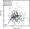 |
Fig. 18 [24] – [70] vs. [70] – [160] color–color diagram including only cores for which 24 μm counterparts exist (black). The high-luminosity sources (L > 103 L⊙) are indicated in green. The typical error is plotted in the lower-left corner. Since very bright sources often saturated the MIPS 24 μm detector, additional data points extracted from the IRAS point source catalog at 25 μm (red diamonds) and the MSX point source catalog at 21 μm (blue triangles) were used in lieu of a MIPS 24 μm data point in this plot. Note that both the IRAS and MSX fluxes were integrated over significantly larger areas corresponding to the beam of the respective telescopes. |
In Table 2, we list the cores above 50 M⊙ that lack a 24 μm counterpart. In Figs. 19 and 20, we show the MIPS 24 μm image and PACS 100 μm image of these four 24 μm-dark cores which are above 50 M⊙ based on our SED models. These sources have dust temperatures between 12 and 17 K and luminosities from 37 to 354 L⊙. In all cases, they are found in the immediate vicinity of cores with a bright 24 μm emission source. In Fig. 21 we show that the diffuse emission, likely due to the nearby source (in some cases HMPO) hampers our sensitivity to 24 μm counterparts for the neighboring cores we feature in Figs. 19 and 20.
IRDC sample.
Observation details.
7.3. Environment of cores
For 44 of the 45 targets, there are sub-millimeter maps which we have used to estimate the total cloud mass from either the ATLASGAL survey, SCUBA archival maps, or published MAMBO 1.2 mm maps (see Sect. 2.3.2 and Table 3). We compute total cloud masses (Mcloud) using these data assuming a single dust temperature of 20 K, as we do not yet have dust temperature maps for the large-scale emission in our sample in order to take into account temperature gradients. We will revisit this added complexity in forthcoming work.
In Fig. 22 we show the mass found in cores as a function of total cloud mass. Clearly, in the clouds of higher mass, there is also more mass in cores. The ISOSS sources are more isolated and, based on the limited SCUBA observations, they have smaller gas reservoirs, which implies that they will likely form lower-mass clusters than the IRDCs. Interestingly, the median fraction of total core mass to total cloud mass is relatively constant at about 10% for all 44 clouds considered.
The 496 cores we report here are not evenly distributed across the sample, with some clouds hosting just one core meeting our criteria, and others hosting over 30. We use a minimum spanning tree algorithm (e.g. Billot et al. 2011) to compute the mean projected core separation for each cloud. Average over the sample, the mean separation is roughly 0.5 pc. We note, however, that because of the strict criteria of our point source extraction, this is certainly an underestimate of the ubiquity and proximity of cores of varying characteristics and evolutionary stages.
What is the difference between IRDCs and ISOSS sources in terms of their core properties? There are a total of 53 cores in the 16 ISOSS targets in our sample (average 3 per ISOSS target), while there are 448 cores in the 29 IRDCs (average 12 cores per IRDC). In Fig. 23 we show the distributions of core properties for the IRDC cores and ISOSS cores. There is no major distinction between the populations, only that the median temperature of ISOSS cores is higher by ~2 K compared to just the IRDC cores, which is not surprising since most of the ISOSS cores are also 24 μm-bright cores, which show a similar median shift compared to the 24 μm-dark population (see Fig. 15).
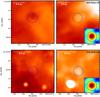 |
Fig. 19 Left panels show the MIPS 24 μm image and the right panels show the PACS 100 μm image of the most massive cores with no 24 μm counterparts which are listed in Table 2. The top row is core 10 in IRDC18454 (estimated 138 M⊙), and the bottom row is core 22 in IRDC18182 (estimated 89 M⊙). The psf of Herschel at 100 μm, rotated in the sense of the scan direction, is shown in the lower-right corner of the right-hand panels. The blue circles indicate the position of the massive core in both the MIPS 24 μm and PACS 100 μm image. |
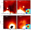 |
Fig. 20 Left panels show the MIPS 24 μm image and the right panels show the PACS 100 μm image of the most massive cores with no 24 μm counterparts which are listed in Table 2. The top row is core 18 in IRDC028.34+0.06 (estimated 53 M⊙), and the bottom row is core 9 in IRDC18223 (estimated 51 M⊙). The psf of Herschel at 100 μm, rotated in the sense of the scan direction, is shown in the lower-right corner of the right panels. The blue circles indicate the position of the massive core in both the MIPS 24 μm and PACS 100 μm image. |
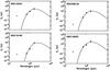 |
Fig. 21 SEDs of massive cores from Fig. 19 (left column) and Fig. 20 (right column). The diamond plotted at the 24 μm position represents an estimate of the local diffuse 24 μm emission due to a nearby bright region. No 24 μm counterpart is reported for any of these sources, but the diffuse emission hampers our ability to detect counterparts for these cores. |
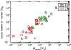 |
Fig. 22 Total mass found in cores versus the total mass of a given cloud, distinguishing between cores found in IRDCs (green) and ISOSS sources (red). |
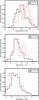 |
Fig. 23 Normalized histograms of the temperatures (top), luminosities (middle), and masses (bottom) of cores found in IRDCs (black) and those in ISOSS sources (red). |
As shown in Fig. 5, the ISOSS sources are our main probe of the outer Galaxy, where the ambient radiation field is lower than in the active Molecular Ring. Still, the cores found in ISOSS targets have higher temperatures and luminosities than average, but essentially the same core masses. Figure 24 shows again the core colors, this time distinguishing between IRDC and ISOSS cores. Here the ISOSS cores are quite confined to blue colors. This implies that the ISOSS cores are not as heavily embedded objects, or that they are more evolved cores.
8. Conclusions
We present an overview of the first results of the Earliest Phases of Star Formation survey with Herschel, focusing on the sample of 45 high-mass regions. The goal of the work presented here is to present the EPoS sample of IRDCs and ISOSS sources as a whole and profile the population of unresolved point sources, which we call cores, within them. We use PACS point source flux densities to construct and fit modified blackbodies to the spectral energy distributions of each core and use the fit to estimate its temperature, luminosity, and mass. The main results of this work are as follows:
-
We extract 496 point sources in the 45 IRDC structures in our sample. Their sizes range from 0.05 to 0.3 pc, which are consistent with “cores” in the global context of star formation (Bergin & Tafalla 2007). We model the SED of the cores based on the 70, 100, and 160 μm point source fluxes. We find a wide range in core luminosities (0.1 to 104 L⊙, median 16 L⊙) and masses (0.1 to a few 103 M⊙, median 4 M⊙). The dust temperatures range from 13 to 30 K (median 20 K).
-
The fluxes at 70, 100, and 160 μm are good predictors of the core luminosity, with the tightest correlation at 160 μm. We perform simple radiative transfer models which show that in cores housing protostars, emission at these wavelengths are determined mainly by the internal source properties. For starless cores, our models show that an amplified external radiation field can cause emission at these wavelengths to reach levels found in protostellar cores. Further work is needed to determine the effects of protostars with various parameters and that of anisotropic heating from neighboring sources.
-
Most (66%) of the cores have a counterpart at 24 μm. Cores with 24 μm counterparts tend to be marginally more massive and more luminous on average than their 24 μm-dark brethren. To the extent which other surveys (e.g. Spitzer and molecular line observations) overlap with our sample, we find that the pre-existing evidence for star formation activity (e.g. YSO colors, outflow activity) almost always coincides with the presence of a 24 μm counterpart, leading us to conclude that such cores contain protostars. Cores without a 24 μm counterpart may also harbor protostars, but have not yet been probed for supporting evidence for embedded sources, or they may be starless cores with some level of external heating. Our radiative transfer models show that external heating is unlikely to account for the 24 μm emission. In order to detect a 24 μm counterpart, the inner core region containing the warm dust heated by an internal protostar must be exposed via a protostellar outflow clearing a cavity in the outer pare. This leads us to conclude that when 24 μm counterparts are detected, it is because a core is in a more evolved state.
-
Cores that have a counterpart at 24 μm are warmer on average than cores without a 24 μm counterpart. We conclude that while the mass and luminosities of these two populations are similar, the warmer cores have protostars that have heated a larger volume of dust within the core, which moderately increases the average core temperature traced by the PACS observations. We find that cores with larger fluxes at 24 μm tend to have higher outer-core temperatures. Warmer cores also correspond to “bluer” colors on the PACS color–color plot ([70] – [100] vs. [100] – [160]).
-
In addition to the 496 cores cataloged in this paper, we find an additional 312 candidate cores which appear only at 100 and 160 μm. We can not model these cores because the SED is too poorly constrained, but we find that their [100] – [160] color is consistent with yet colder dust temperatures, thus these may represent an evolutionary stage prior to protostellar formation and require further follow-up observations to model.
-
The cores are warmer than typical temperatures of large-scale cloud structures in which they are embedded. We conclude that at PACS wavelengths, the core fluxes are due to the effects of internal heating sources and heating from the external radiation field does not play a significant role. We emphasize here that since we probe on core scales where the cores are embedded in high column density structures which shield them from the ambient radiation field. Further modelling of the dust temperature and column density structure on the “clump” and “cloud” scales will enable us to determine more precisely on what scales temperature gradients caused by external heating play an important role.
-
Cores within ISOSS sources tend to be 24 μm-bright and less massive than cores in IRDCs. They serve as our probes of cores in the outer Galaxy, where we are biased against finding “dark clouds” in the same sense as IRDCs in the inner-Galaxy. As molecular gas is known to be more concentrated in the inner Molecular Ring of the Galaxy, these sources offer unique insight into the early phases of isolated “massive” star formation.
The legacy of the EPoS data will reach far beyond the overview presented here. In this paper, we focus on the core population, much of which was until now completely obscured by heavy extinction. These embedded cores will play a role in the further interpretation of the EPoS data, which will include a full treatment of the radiative transfer from the small to large scales. Future work will also address the detailed large-scale structure in dust temperature and column density, which together can better characterize the environments of the embedded cores.
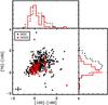 |
Fig. 24 PACS color plot of IRDC cores (black) and ISOSS cores (red). |
Online material
Appendix A: Individual target descriptions
IRDCs were discovered and subsequently named based on their appearance in absorption against the bright Galactic background at 8 μm and 15 μm based on Galactic plane surveys almost two decades ago. The follow-up studies focused on IRDCs which were largest and most easily identifiable in contrast: those lying in the inner Galaxy. Because most millimeter facilities at the time were located in the northern hemisphere, detailed work was done preferentially on IRDCs in the first quadrant of the Galaxy, which is reflected in the fact that much of our selection of “well-studied” sources are found in the first quadrant. For the EPoS sample, we selected IRDCs from these various surveys, favoring the targets that are relatively nearby (d < 5 kpc). They are denoted as IRDC LLL.LL-B.BB in our catalog, where “L” and “B” are the Galactic longitude and latitude.
Another strategy utilized in selecting IRDCs takes advantage of the fact that high-mass star formation is known to occur in a clustered mode, and there is ample evidence for triggering of several generations of high-mass star formation (e.g. Deharveng et al. 2010), thus a portion of our sample is comprised of infrared-dark regions found in millimeter surveys near known high-mass protostellar objects (HMPOs, Sridharan et al. 2002; Beuther et al. 2002a–d). Sridharan et al. (2005) correlated the 1.2 mm bolometer data from a well-studied HMPO sample with the corresponding MSX mid-infrared data. Within the 69 studied fields they found 56 gas clumps with associated mid-infrared shadows (Sridharan et al. 2005), most of them with masses in excess of several 100 M⊙ and temperatures on the order of ~15 K (Sridharan et al. 2005). Follow-up observations revealed outflow activity – indicating already ongoing early star formation – in ~40% of the sources, and dense gas abundances (e.g., CH3OH and CH3CN) are similar to those of low-mass starless cores (Beuther & Sridharan 2007).
Using the 170 μm ISOPHOT (Lemke et al. 1996) Serendipity Survey (ISOSS Bogun et al. 1996), we selected 16 candidates for massive (M > 100 M⊙), cold (Tdust < 18 K) objects based on preliminary studies (Krause et al. 2003, 2004; Birkmann et al. 2007). For these sources, the naming convention derives from the FK5 (J2000) coordinates, r for right ascension and d for declination, represented as ISOSSJrrrrr ± dddd. As shown in Fig. 1, these objects represent the bulk of the objects from the outer Galaxy, which will have characteristically lower infrared background emission. The ISOSS sample has a large range in distances, but the median distance, 3.52 kpc, is only slightly higher than the median distance of the sample, 3.23 kpc.
IRDC 004.36-0.06: Hennebelle et al. (2001) first identified this source as a peak in the extinction from ISOGAL observations. Teyssier et al. (2002) detect 13CO and strong C18O emission associated with this sources.
IRDC 009.86-0.04: Another inner-Galaxy object from Hennebelle et al. (2001) that exhibits strong CO emission in Teyssier et al. (2002). Ragan et al. (2006) conducted further molecular studies on this IRDC, detecting N2H+ (1−0) and widespread CS(2−1) emission at the same velocity as Teyssier et al. (2002). Ragan et al. (2006) find a cloud mass of 1500 M⊙ based on the integrated map of N2H+ emission. Ragan et al. (2009) present Spitzer observations of this cloud. There are 31 YSOs in the vicinity of this cloud, two of which are classified in the earliest embedded phase.
IRDC 010.70-0.13: Carey et al. (2000) conduct continuum observations of this target and find a bright, compact source. Peretto & Fuller (2009) find nine fragments within this IRDC.
IRDC 011.11-0.12: This was one of the first IRDCs subject to intense study in the literature, first in the infrared (Carey et al. 1998), the millimeter (Carey et al. 2000; Johnstone et al. 2003), and in molecular line emission (Pillai et al. 2006a,b). The filament is about ~20 pc long consisting of over 1800 M⊙ (from 8 μm extinction measurements), and the bulk of the gas has an average kinetic temperature of 12 K.
This object was observed as part of the Herschel science demonstration phase, and Henning et al. (2010) present the continuum properties of the pre- and proto-stellar cores uncovered at PACS wavelengths.
IRDC 013.90-0.51: Peretto & Fuller (2009) identify this object as a Spitzer dark core, and Vasyunina et al. (2009) perform 1.2 mm continuum observations showing it breaks into four main peaks. The southern-most source (P3) showed double-peaked molecular line profiles in Vasyunina et al. (2011) indicating either the presence of two components superimposed along the line of sight or internal motion within the cloud.
IRDC 015.05+0.09: Hennebelle et al. (2001) and Teyssier et al. (2002) identify this object as one of the most opaque objects, which results in depletion of the CO isotopomers onto the dust grains. Rathborne et al. (2006) find that this IRDC, with a total mass of 158 M⊙, resolves into five 1.2 mm flux peaks with masses of 105, 83, 22, 43, and 29 M⊙, assuming 15 K dust. Wang et al. (2006) report water maser associated with MM1 (of Rathborne et al. 2006).
IRDC 019.30+0.07: This source was targeted in Carey et al. (1998, 2000) detected in H2CO and SCUBA 450/850 μm surveys, indicating two main spatial peaks in emission. Pillai et al. (2006a) confirm this morphology in NH3 emission, find gas temperatures of 18.4 and 14.3 K, and masses of 893 and 823 M⊙ for these regions. Rathborne et al. (2006) find a total mass of 3168 M⊙ for the entire complex, though much lower masses (113 and 114 M⊙) for the two respective peaks. Finally, Devine et al. (2011) find a total mass of 1130 M⊙, concentrated in four NH3 clumps.
IRDC 028.34+0.06: Of all the sources in Carey et al. (2000), IRDC028.34+0.06 shows the strongest submillimeter emission (in two primary peaks at 450 and 850μm) and, thus, has the greatest estimated mass (up to several hundred M⊙ each depending on the choice of dust emissivity index, β). Pillai et al. (2006a) examine this source, here resolving into five subregions in NH3 emission, with temperatures ranging from 13.2 to 16.6 K and total mass of 4263 M⊙ (from ammonia measurements). Observations by Rathborne et al. (2006) at 1.2 mm find a total cloud mass of 15 895 M⊙ (the most massive in their sample) and resolve this target into 18 peaks. In three of those peaks (MM4, MM6, and MM9), Wang et al. (2006) detect water masers. Wang et al. (2008) perform high resolution observations in NH3, linking the presence of embedded protostars to the enhancement of linewidth and an increase in rotation temperature. Zhang et al. (2009) obtain SMA continuum and spectral line observations, further resolving the dominant cores into multiple substructures.
IRDC 048.66-0.29: Situated close to the GMC complex W51, this IRDC was targeted for SCUBA 450 and 850 μm and HCO+(3−2) observations by Ormel et al. (2005). They found that (at the resolution of the JCMT) this IRDC broke into three cores (P1, P2, and EP) near 100 M⊙ each, and the line data show that (intermediate mass) star formation is ongoing within the cores. Rathborne et al. (2006) surveyed this IRDC with 1.2 mm continuum observations, reporting a total cloud mass of 917 M⊙ for the cloud and 52 and 39 M⊙ masses for the dark cores reported in Ormel et al. (2005), though the core sizes in Rathborne et al. (2006) are considerably smaller, which could account for the difference. The star forming properties were studied in detail with Spitzer in van der Wiel & Shipman (2008), in which 13 YSOs were identified near the cloud. The Spitzer observations also resolved P1 (from Ormel et al. 2005) into two peaks, but found the star formation properties to be consistent.
IRDC 079.31+0.36: This IRDC is among the nearest in our sample and was first observed by Carey et al. (2000). Redman et al. (2003) characterize the ongoing star formation in this IRDC which may have been triggered. Pillai et al. (2006a) find high column densities (>1023 cm-3) and gas tempertatures between 12 and 15 K in this region. This object was included in the SCUBPOL legacy survey Matthews et al. (2009).
IRDC 310.39-0.30: Vasyunina et al. (2009) find the millimeter continuum emission peak coincides with the absorption peak in the mid-infrared, from which they estimate the mass is 1320 M⊙. The continuum peak is stronger in the MIR dark source than for the nearby MIR-bright source, indicating that this IRDC could contain a range of evolutionary stages. The MIR-bright sources are included in the Cyganowski et al. (2008) EGO catalog, and Vasyunina et al. (2011) detect weak SiO emission in this IRDC.
IRDC 316.72+0.07: This object hosts a small cluster of embedded infrared sources and has a mass between 400 and 950 M⊙ derived from 8 μm extinction (Linz et al. 2007), or 561 M⊙ based on 1.2 mm emission.
IRDC 320.27+0.29: This cloud is comprised of a compact eastern component and an elongated western cloud, which are 50 and 70 M⊙, respectively, based on 1.2 mm continuum observations (Vasyunina et al. 2009). Molecular line emission observed by Vasyunina et al. (2011) is weak.
IRDC 321.73+0.05: Two main clumps of approximately equal mass (about 100 M⊙Vasyunina et al. 2009) comprise this IRDC. The eastern source, with a column density of 3.2 × 1022 cm-2, shows a weak source at 24 μm, yet Vasyunina et al. (2011) detect SiO and asymmetric HCO+ emission, indicating the presence of a shock and inflowing gas, both indicators of star formation activity at an early stage. The western source also exhibits multiple peaks in the molecular line emission attributed to complex internal motions throughout the cloud.
HMSC 07029: The clump HMSC07029 (a.k.a. UYSO 1) had been recognised as a distinct peak in a (sub-)millimeter survey of massive protocluster-cores in the outer galaxy by Klein et al. (2005). It is a distinct intermediate-mass core clearly offset from the neighboring IRAS source 07029-1215 which in the pre-Spitzer era was just detectable at wavelengths ≥ 450 μm citepForbrich2004. However, strong CO outflow activity is also associated with this core. Forbrich et al. (2009) collected more data on this source and revealed an impressive system of crossed Hs shocked emission jets apparently emanating from the core which in Spitzer 70 μm images was 10′′ offset from the interferometric position in the millimeter. Our EPoS Herschel data could eventually disentangle the 70 μm peak position which is coinciding with the interferometric position, from the surrounding extended PDR emission. More details about this enigmatic region are given in our A&A special issue paper (Linz et al. 2010).
IRDC 18102: Although originally selected as a high-mass protostellar object (HMPO), the singular 1.2 mm continuum peak (Beuther et al. 2002b) in this regions turns out to be mid-infrared dark in MSX and offset by less than 1′ from an infrared-bright and centimeter-bright ultracompact Hii region. SiO emission, known to be associated with molecular outflows, is reported in Beuther & Sridharan (2007) associate with the millimeter continuum peak. Since the infrared-dark and bright regions are in so close proximity, interaction between the different evolutionary stages is expected.
IRDC 18151: The name-giving IRAS 18151-1208 is a well-known high-mass outflow-disk region (Davis et al. 2004; Fallscheer et al. 2011). In the vicinity of this active site, one finds two similarly massive gas-clumps of which the one is 8 μm-dark and hosts a H2O maser (Beuther et al. 2002d).
IRDC 18182: The central IRAS 18182-1433 is a well-known “hot core”-type high-mass star-forming region (Zapata et al. 2006; Beuther et al. 2006). The infrared-dark gas-clumps are found approximately 2′ to the southeast and northeast.
IRDC 18223: This filamentary dark cloud is located directly south of the luminous IRAS 18223-1243. The region contains regions is several evolutionary stages, from IRDCs with already embedded ongoing star formation (e.g. IRDC 18223-3 Beuther et al. 2005b; Beuther & Steinacker 2007; Fallscheer et al. 2009) to potentially real high-mass starless cores that are even dark at 70 μm (Beuther et al. 2010).
IRDC 18306: About 2′ offset to the northeast from the central IRAS 18306-0835 we find filamentary infrared-dark structures that are associated with millimeter continuum emission, broken into three main 1.2 mm peaks.
IRDC 18308: Again we find filamentary, mid-infrared dark millimeter continuum structures extending from IRAS 18308-0841 toward the north and containing five main 1.2 mm peaks.
IRDC 18310: This region hosts Hii region, IRAS 18310-0825, a compact mid-infrared-dark filament, totalling five distinct millimeter continuum peaks.
IRDC 18337: This region contains three strong 1.2 mm continuum sources that appear to be laid out in a linear structure. While the IRAS 18337-0743 has strong mid-infrared emission, the second source is still – although weaker – mid-infrared bright, and the third source is mid-infrared dark. This region is likely a particularly good candidate to investigate sequential star formation.
IRDC 18385: A 2′ millimeter continuum filament stems from IRAS 18385-0512, and an isolated infrared-dark globule lies to the south east.
IRDC 18437: This region contains a chain of millimeter continuum sources, including IRAS 18437-0216, in approximate north-south direction with different degrees of associated mid-infrared emission. Polarized sub-millimeter continuum emission is observed by Matthews et al. (2009).
IRDC 18454: This complex of several millimeter continuum sources is located at the north-eastern edge of the prominent Galactic mini-starburst W43 (Motte et al. 2003; Bally et al. 2010; Nguyên Lu’O’Ng et al. 2011) at the same systemic velocity, thus, at presumably the same distance. The millimeter continuum sources exhibit several velocity components. Beuther et al. (2012) explore whether these are due to chance projections or physical interactions. Furthermore, it is in general interesting to find infrared dark massive gas clumps in so close proximity to one of the most active star-forming regions in our Galaxy.
IRDC 18530: Extending about 3′ south of IRAS 18530+0215 one finds a filamentary infrared-dark structure that is associated with millimeter continuum emission.
IRDC 19175: This regions hosts a spiral-like filamentary structure extending several arc-minutes from IRAS 19175+1357 distributed in seven 1.2 mm clumps. Two of the mid-infrared dark gas clumps have already been studied by Beuther & Henning (2009) who found many smaller sub-structures within them.
IRDC 20081: IRAS 20081+2720 lies at the center of a compact infrared-dark filament with two compact 1.2 mm peaks to the north and south.
ISOSS sources
The ISOSS portion of the sample lies largely in the outer Galaxy, thus there are fewer detailed studies in the literature to date. In many cases a nearby (possibly associated) IRAS source was included in a maser survey. These resulted in non-detections in most cases, but we list the exceptions below along with the descriptions of the few detailed studies.
ISOSSJ04225+5150: Birkmann (2006, PhD) found three compact cores in this region. The first core (SMM1) has a mass of 275 M⊙ and a temperature of 21.4 K. The most massive core (SMM3, 510 M⊙, 17 K) show indications for shocked outflows and an associated PDR (Pitann et al. 2011).
ISOSSJ06527+0140:Migenes et al. (1999) and Sunada et al. (2007) detect a water maser at the position of IRAS source IRAS 06501+0143.
ISOSSJ18364-0221:Birkmann et al. (2006) found that ISOSS J18364-0221 broke into two compact cores (SMM1 and SMM2). SMM1 is a protostellar core (16.5 K, 75 M⊙) with energetic outflows. The second core (SMM2) is a more massive (280 M⊙), pre-stellar object of lower temperature (12 K).
Hennemann et al. (2009) performed follow-up millimeter continuum and molecular line observations of SMM1 and found it was actually comprised of two sub-clumps (SMM1 North and South). While SMM1 South is detected at 24 and 70 μm and SMM1 North is undetected in the infrared, both are associated with molecular outflows reaching up to 4.6 pc from the core.
ISOSSJ19357+1950: SCUBA observations (Hennemann et al. 2008) reveal three resolved clumps at 450 μm: SMM1 North (0.37 pc, 70 M⊙) and South (0.31 pc, 50 M⊙), and SMM2 in the South-West (0.39 pc, 120 M⊙). SMM2 hosts a deeply embedded protostellar object that may evolve to a massive YSO.
ISOSSJ19486+2556:Hennemann et al. (2008) find three submillimeter clumps (SMM1-3) in this region, located along a chain from North-East to South-West. SMM2 and SMM3 are associated with bright 24 and 70 μm sources and have masses of 40 and 60 M⊙, whereas SMM1 (100 M⊙) is not detected with Spitzer.
ISOSSJ20153+3453: A single core with a gas mass of ~120 M⊙ and a dust temperature of 17 K was identified in this region by Hennemann et al. (2008). Two neighboring mid-infrared sources are detected towards SMM1, the one towards the submillimeter peak is interpreted as embedded YSO that is actively accreting as suggested by the presence of “fuzzy” emission prominent at 4.5 μm. Futher Spitzer observations indicate the presence of a PDR. Excited gas suggests shocked outflows in this region (Pitann et al. 2011).
ISOSSJ20298+3559: This region harbors four submillimeter clumps SMM1-4 and has been studied in detail in Krause et al. (2003) except for SMM4 which is offset to the west. SMM1 (0.14 pc, 10 M⊙) and SMM2 (unresolved: 0.07 pc, 3 M⊙) are joined by extended submillimeter emission. SMM4 is more extended (0.34 pc, 60 M⊙) than the other clumps. SMM1 hosts an embedded intermediate-mass YSO, and a Class II-like intermediate-mass YSO is associated with SMM4 (Hennemann et al. 2008).
ISOSSJ22478+6357: An elongated clump (SMM1) is resolved in both an Eastern (0.14 pc, 60 M⊙) and a Western component (0.24 pc, 120 M⊙) at 450 μm. Towards SMM1 East, a Class II-like YSO of intermediate central mass has been identified among several 24 μm sources (Hennemann et al. 2008).
ISOSSJ23053+5953:Birkmann et al. (2007) identified two cores in this region with ~200 M⊙ each (at 19.5 K and 17.3 K). HCO+ kinematics indicate in-falling gas in both cores. Several outflow features were found in this region by interferometric, spectroscopic and NIR narrow-band observations (see Birkmann et al. 2007; Pitann et al. 2011).
Appendix B: Images
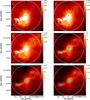 |
Fig. B.1 The Herschel a) PACS 70 μm, b) PACS 100 μm, c) PACS 160 μm, d) SPIRE 250 μm, e) SPIRE 350 μm, and f) SPIRE 500 μm images of HMSC 07029. The flux scales on the right edge of each PACS panel are in Jy pixel-1 and Jy beam-1 for the SPIRE panels. Point sources are marked with a blue × , and the white solid line marks the boundary defined in Sect. 2.3.2. Cyan contours on the SPIRE panels show SCUBA 850 μm emission from 20% of peak flux in increments of 10%: 0.32, 0.49, 0.65, 0.81, 0.97, 1.13, 1.30, 1.46, 1.62 Jy beam-1. |
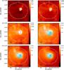 |
Fig. B.2 Same image layout as Fig. B.1 but for IRDC 310.39-0.30. Cyan contours on the SPIRE panels d)–f) show ATLASGAL 870 μm: 0.3, 0.45, 0.6, 0.75, 0.9, 1.05, 1.2, 1.35, 1.5 Jy beam-1. |
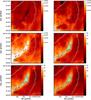 |
Fig. B.3 Same image layout as Fig. B.1 but for IRDC 316.72+0.07. Cyan contours on the SPIRE panels d)–f) show ATLASGAL 870 μm: 0.4, 0.6, 0.8, 1.0, 1.2, 1.4, 1.6, 1.8, 2.0 Jy beam-1. |
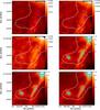 |
Fig. B.4 Same image layout as Fig. B.1 but for IRDC 320.27+0.29. Cyan contours on the SPIRE panels d)–f) show ATLASGAL 870 μm: 0.2, 0.3, 0.4, 0.5, 0.6, 0.7, 0.8, 0.9, 1.0 Jy beam-1. |
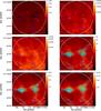 |
Fig. B.5 Same image layout as Fig. B.1 but for IRDC 321.73+0.05. Cyan contours on the SPIRE panels d)–f) show MAMBO 1.2 mm: 0.06, 0.09, 0.12, 0.18, 0.21, 0.24, 0.27, 0.3 Jy beam-1. |
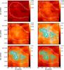 |
Fig. B.6 Same image layout as Fig. B.1 but for IRDC 004.36-0.06. Cyan contours on the SPIRE panels d)–f) show ATLASGAL 870 μm: 0.07, 0.11, 0.14, 0.18, 0.21, 0.25, 0.28, 0.32, 0.35 Jy beam-1. |
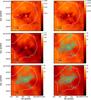 |
Fig. B.7 Same image layout as Fig. B.1 but for IRDC 009.86-0.04. Cyan contours on the SPIRE panels d)–f) show ATLASGAL 870 μm: 0.08, 0.13, 0.168, 0.21, 0.25, 0.29, 0.34, 0.38, 0.42 Jy beam-1. |
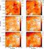 |
Fig. B.8 Same image layout as Fig. B.1 but for IRDC 010.70-0.13. Cyan contours on SPIRE panels d)–f) show ATLASGAL 870 μm: 0.39, 0.59, 0.78, 0.98, 1.17 , 1.37, 1.56, 1.76, 1.95 Jy beam-1. |
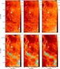 |
Fig. B.9 Same image layout as Fig. B.1 but for IRDC 011.11-0.12. Cyan contours on the SPIRE panels d)–f) show ATLASGAL 870 μm: 0.34, 0.51, 0.68, 0.85, 1.02, 1.19, 1.36, 1.53, 1.7 Jy beam-1. |
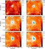 |
Fig. B.10 Same image layout as Fig. B.1 but for IRDC 18102. Cyan contours on the SPIRE panels d)–f) show ATLASGAL 870 μm: 0.68, 1.03, 1.37, 1.71, 2.05, 2.40, 2.74, 3.08 Jy beam-1. |
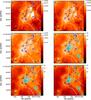 |
Fig. B.11 Same image layout as Fig. B.1 but for IRDC 013.90-0.51. Cyan contours on the SPIRE panels d)–f) show ATLASGAL 870 μm: 0.25, 0.37, 0.50, 0.62, 0.74, 0.87, 0.99, 1.12, 1.24 Jy beam-1. |
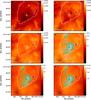 |
Fig. B.12 Same image layout as Fig. B.1 but for IRDC 015.05+0.09. Cyan contours on the SPIRE panels d)–f) show ATLASGAL 870 μm: 0.08, 0.13, 0.17, 0.21, 0.25, 0.29, 0.34, 0.38, 0.42 Jy beam-1. |
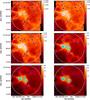 |
Fig. B.13 Same image layout as Fig. B.1 but for IRDC 18151. Cyan contours on the SPIRE panels d)–f) show MAMBO 1.2 mm: 0.13, 0.20, 0.27, 0.35, 0.40, 0.47, 0.54, 0.61, 0.67 Jy beam-1. |
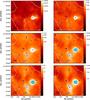 |
Fig. B.14 Same image layout as Fig. B.1 but for IRDC 18182.Cyan contours on the SPIRE panels d)–f) show ATLASGAL 870 μm: 0.6, 0.9, 1.2, 1.5, 1.8, 2.1, 2.4, 2.7, 3.0 Jy beam-1. |
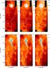 |
Fig. B.15 Same image layout as Fig. B.1 but for IRDC 18223. Cyan contours on the SPIRE panels d)–f) show ATLASGAL 870 μm: 0.49, 0.74, 0.99, 1.24, 1.48, 1.73, 1.98, 2.22, 2.47 Jy beam-1. |
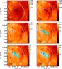 |
Fig. B.16 Same image layout as Fig. B.1 but for IRDC 19.30+0.07. Cyan contours on the SPIRE panels d)–f) show ATLASGAL 870 μm: 0.25, 0.37, 0.50, 0.62, 0.74, 0.87, 0.99, 1.12, 1.24 Jy beam-1. |
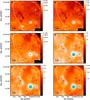 |
Fig. B.17 Same image layout as Fig. B.1 but for IRDC 18306. Cyan contours on the SPIRE panels d)–f) show ATLASGAL 870 μm: 0.4, 0.6, 0.8, 1.0, 1.2, 1.4, 1.6 ,1.8, 2.0 Jy beam-1. |
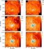 |
Fig. B.18 Same image layout as Fig. B.1 but for IRDC 18308. Cyan contours on the SPIRE panels d)–f) show ATLASGAL 870 μm: 0.4, 0.6, 0.8, 1.0, 1.2, 1.4, 1.6 ,1.8, 2.0 Jy beam-1. |
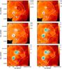 |
Fig. B.19 Same image layout as Fig. B.1 but for IRDC 18310. Cyan contours on the SPIRE panels d)–f) show ATLASGAL 870 μm: 0.4, 0.6, 0.8, 1.0, 1.2, 1.4, 1.6 ,1.8, 2.0 Jy beam-1. |
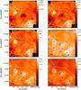 |
Fig. B.20 Same image layout as Fig. B.1 but for IRDC 18337. Cyan contours on the SPIRE panels d)–f) show ATLASGAL 870 μm: 0.4, 0.6, 0.8, 1.0, 1.2, 1.4, 1.6 ,1.8, 2.0 Jy beam-1. |
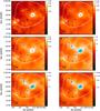 |
Fig. B.21 Same image layout as Fig. B.1 but for IRDC 18385. Cyan contours on the SPIRE panels d)–f) show ATLASGAL 870 μm: 0.4, 0.6, 0.8, 1.0, 1.2, 1.4, 1.6 ,1.8, 2.0 Jy beam-1. |
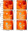 |
Fig. B.22 Same image layout as Fig. B.1 but for IRDC 028.34+0.06. Cyan contours on the SPIRE panels d)–f) show ATLASGAL 870 μm: 0.8, 1.2, 1.6, 2.0, 2.4, 2.8, 3.2, 3.6, 4.0 Jy beam-1. |
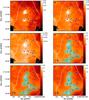 |
Fig. B.23 Same image layout as Fig. B.1 but for IRDC 18437. Cyan contours on the SPIRE panels d)–f) show ATLASGAL 870 μm: 0.2, 0.3, 0.4, 0.5, 0.6, 0.7, 0.8, 0.9, 1.0 Jy beam-1. |
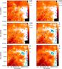 |
Fig. B.24 Same image layout as Fig. B.1 but for IRDC 18454. Cyan contours on the SPIRE panels d)–f) show ATLASGAL 870 μm: 2.0, 3.0, 4.0, 5.0, 6.0, 7.0, 8.0, 9.0, 10.0 Jy beam-1. |
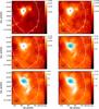 |
Fig. B.25 Same image layout as Fig. B.1 but for IRDC 18530. Cyan contours on the SPIRE panels d)–f) show ATLASGAL 870 μm: 0.6, 0.9, 1.2, 1.5, 1.8, 2.1, 2.4, 2.7, 3.0 Jy beam-1. |
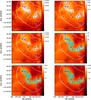 |
Fig. B.26 Same image layout as Fig. B.1 but for IRDC 19175. Cyan contours on the SPIRE panels d)–f) show ATLASGAL 870 μm: 0.19, 0.29, 0.38, 0.48, 0.57, 0.67, 0.76, 0.86, 0.95 Jy beam-1. |
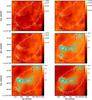 |
Fig. B.27 Same image layout as Fig. B.1 but for IRDC 048.66-0.29. Cyan contours on the SPIRE panels d)–f) show ATLASGAL 870 μm: 0.106, 0.159, 0.21, 0.265, 0.318, 0.371, 0.424, 0.477, 0.53 Jy beam-1. |
 |
Fig. B.28 Same image layout as Fig. B.1 but for IRDC 20081. Cyan contours on the SPIRE panels d)–f) show MAMBO 1.2 mm: 0.04, 0.07, 0.09, 0.11, 0.13, 0.14, 0.16, 0.18 Jy beam-1. |
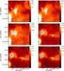 |
Fig. B.29 Same image layout as Fig. B.1 but for IRDC 079.31+0.36. Cyan contours on the SPIRE panels d)–f) show SCUBA 850 μm: 1.0, 1.5, 2.0, 2.5, 3.0, 3.5, 4.0, 4.5, 5.0 Jy beam-1. |
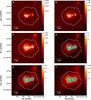 |
Fig. B.30 Same image layout as Fig. B.1 but for ISOSS J04225+5150. Cyan contours on the SPIRE panels d)–f) show SCUBA 850 μm: 0.22, 0.32, 0.43, 0.54, 0.65, 0.76, 0.86, 0.97, 1.08 Jy beam-1. |
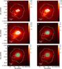 |
Fig. B.32 Same image layout as Fig. B.1 but for ISOSS J06527+0140. Cyan contours on the SPIRE panels d)–f) show SCUBA 850 μm: 0.41, 0.62, 0.82, 1.03, 1.24, 1.44, 1.65, 1.85, 2.06 Jy beam-1. |
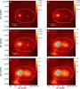 |
Fig. B.33 Same image layout as Fig. B.1 but for ISOSS J18364-0221. Cyan contours on the SPIRE panels d)–f) show SCUBA 850 μm: 0.21, 0.31, 0.42, 0.52, 0.63, 0.73, 0.83, 0.94, 1.04 Jy beam-1. |
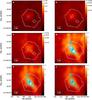 |
Fig. B.34 Same image layout as Fig. B.1 but for ISOSS J19357+1950. Cyan contours on the SPIRE panels d)–f) show SCUBA 850 μm: 0.06, 0.09, 0.12, 0.15, 0.17, 0.20, 0.23, 0.26, 0.29 Jy beam-1. |
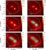 |
Fig. B.35 Same image layout as Fig. B.1 but for ISOSS J19486+2556. Cyan contours on the SPIRE panels d)–f) show SCUBA 850 μm: 0.07, 0.11, 0.14, 0.18, 0.22, 0.25, 0.29, 0.32, 0.36 Jy beam-1. |
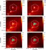 |
Fig. B.36 Same image layout as Fig. B.1 but for ISOSS J19557+2825. Cyan contours on the SPIRE panels d)–f) show SCUBA 850 μm: 0.13, 0.19, 0.26, 0.32, 0.38, 0.45, 0.51, 0.58, 0.64 Jy beam-1. |
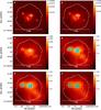 |
Fig. B.37 Same image layout as Fig. B.1 but for ISOSS J20093+2729. Cyan contours on the SPIRE panels d)–f) show SCUBA 850 μm: 0.05, 0.08, 0.10, 0.13, 0.15, 0.18, 0.20, 0.23, 0.25 Jy beam-1. |
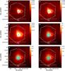 |
Fig. B.38 Same image layout as Fig. B.1 but for ISOSS J20153+3453. Cyan contours on the SPIRE panels d)–f) show SCUBA 850 μm: 0.28, 0.41, 0.55, 0.69, 0.83, 0.97, 1.10, 1.24, 1.38 Jy beam-1. |
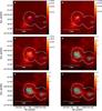 |
Fig. B.39 Same image layout as Fig. B.1 but for ISOSS J20298+3559. Cyan contours on the SPIRE panels d)–f) show SCUBA 850 μm: 0.08, 0.12, 0.20, 0.24, 0.28, 0.32, 0.36, 0.40 Jy beam-1. |
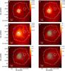 |
Fig. B.40 Same image layout as Fig. B.1 but for ISOSS J21311+5127. Cyan contours on the SPIRE panels d)–f) show SCUBA 850 μm: 0.12, 0.18, 0.24, 0.30, 0.36, 0.42, 0.48, 0.54, 0.60 Jy beam-1. |
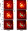 |
Fig. B.41 Same image layout as Fig. B.1 but for ISOSS J22164+6003. Cyan contours on the SPIRE panels d)–f) show SCUBA 850 μm: 0.08, 0.12, 0.20, 0.24, 0.28, 0.32, 0.36, 0.40 Jy beam-1. |
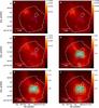 |
Fig. B.42 Same image layout as Fig. B.1 but for ISOSS J22478+6357. Cyan contours on the SPIRE panels d)–f) show SCUBA 850 μm: 0.11, 0.17, 0.22, 0.28, 0.34, 0.39, 0.45, 0.50, 0.56 Jy beam-1. |
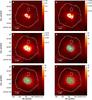 |
Fig. B.43 Same image layout as Fig. B.1 but for ISOSS J23053+5953. Cyan contours on the SPIRE panels d)–f) show SCUBA 850 μm: 0.4, 0.6, 0.8, 1.0, 1.2, 1.4, 1.6, 1.8, 2.0 Jy beam-1. |
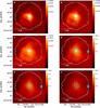 |
Fig. B.44 Same image layout as Fig. B.1 but for ISOSS J23129+5944. Cyan contours on the SPIRE panels d)–f) show SCUBA 850 μm: 0.14, 0.21, 0.28, 0.35, 0.42, 0.49, 0.56, 0.63, 0.70 Jy beam-1. |
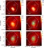 |
Fig. B.45 Same image layout as Fig. B.1 but for ISOSS J23287+6039. Cyan contours on the SPIRE panels d)–f) show SCUBA 850 μm: 0.08, 0.12, 0.20, 0.24, 0.28, 0.32, 0.36, 0.40 Jy beam-1. |
Appendix C: Core catalog
Point sources.
We note that recent observations (Peretto et al. 2010; Beuther et al. 2012) have shown that IRDCs may exhibit temperature gradients, especially when situated near a star forming region. In future work, we shall investigate the degree of this effect throughout the sample making use of more detailed dust temperature maps.
Alternatively, the IRAS 25 μm flux density or MSX 21 μm flux density is given in Table C.1 if MIPS 24 μm is saturated at the position.
Available from http://www.ita.uni-heidelberg.de/~dullemond/software/transphere/
Throughout the text, when we refer to an object having a 24 μm counterpart, we also are referring to objects showing IRAS/25 μm or MSX/21 μm counterparts.
Acknowledgments
This work was supported by the Deutsche Forschungsgemeinschaft priority program 1573 (“Physics of the Interstellar Medium”). PACS has been developed by a consortium of institutes led by MPE (Germany) and including UVIE (Austria); KU Leuven, CSL, IMEC (Belgium); CEA, LAM (France); MPIA (Germany); INAF-IFSI/OAA/OAP/OAT, LENS, SISSA (Italy); IAC (Spain). This development has been supported by the funding agencies BMVIT (Austria), ESA-PRODEX (Belgium), CEA/CNES (France), DLR (Germany), ASI/INAF (Italy), and CICYT/MCYT (Spain). SPIRE has been developed by a consortium of institutes led by Cardiff University (UK) and including Univ. Lethbridge (Canada); NAOC (China); CEA, LAM (France); IFSI, Univ. Padua (Italy); IAC (Spain); Stockholm Observatory (Sweden); Imperial College London, RAL, UCL-MSSL, UKATC, Univ. Sussex (UK); and Caltech, JPL, NHSC, Univ. Colorado (USA). This development has been supported by national funding agencies: CSA (Canada); NAOC (China); CEA, CNES, CNRS (France); ASI (Italy); MCINN (Spain); SNSB (Sweden); STFC (UK); and NASA (USA). This research has made use of NASAs Astrophysics Data System, as well as the SIMBAD database, operated at CDS, Strasbourg, France. This research made use of Tiny Tim/Spitzer, developed by John Krist for the Spitzer Science Center. The Center is managed by the California Institute of Technology under a contract with NASA.
References
- André, P., Ward-Thompson, D., & Barsony, M. 1993, ApJ, 406, 122 [NASA ADS] [CrossRef] [Google Scholar]
- Arce, H. G., Shepherd, D., Gueth, F., et al. 2007, Protostars and Planets V, 245 [Google Scholar]
- Bally, J., Anderson, L. D., Battersby, C., et al. 2010, A&A, 518, L90 [Google Scholar]
- Bergin, E. A., & Tafalla, M. 2007, ARA&A, 45, 339 [NASA ADS] [CrossRef] [Google Scholar]
- Beuther, H., Churchwell, E. B., McKee, C. F., & Tan, J. C. 2007, Protostars and Planets V, 165 [Google Scholar]
- Beuther, H., & Henning, T. 2009, A&A, 503, 859 [NASA ADS] [CrossRef] [EDP Sciences] [Google Scholar]
- Beuther, H., & Sridharan, T. K. 2007, ApJ, 668, 348 [NASA ADS] [CrossRef] [Google Scholar]
- Beuther, H., & Steinacker, J. 2007, ApJ, 656, L85 [NASA ADS] [CrossRef] [Google Scholar]
- Beuther, H., Schilke, P., Gueth, F., et al. 2002a, A&A, 387, 931 [NASA ADS] [CrossRef] [EDP Sciences] [Google Scholar]
- Beuther, H., Schilke, P., Menten, K. M., et al. 2002b, ApJ, 566, 945 [NASA ADS] [CrossRef] [Google Scholar]
- Beuther, H., Schilke, P., Sridharan, T. K., et al. 2002c, A&A, 383, 892 [NASA ADS] [CrossRef] [EDP Sciences] [Google Scholar]
- Beuther, H., Walsh, A., Schilke, P., et al. 2002d, A&A, 390, 289 [NASA ADS] [CrossRef] [EDP Sciences] [Google Scholar]
- Beuther, H., Schilke, P., Menten, K. M., et al. 2005a, ApJ, 633, 535 [NASA ADS] [CrossRef] [Google Scholar]
- Beuther, H., Sridharan, T. K., & Saito, M. 2005b, ApJ, 634, L185 [NASA ADS] [CrossRef] [Google Scholar]
- Beuther, H., Zhang, Q., Sridharan, T. K., Lee, C., & Zapata, L. A. 2006, A&A, 454, 221 [NASA ADS] [CrossRef] [EDP Sciences] [Google Scholar]
- Beuther, H., Henning, T., Linz, H., et al. 2010, A&A, 518, L78 [NASA ADS] [CrossRef] [EDP Sciences] [Google Scholar]
- Beuther, H., Tackenberg, J., Linz, H., et al. 2012, A&A, 538, A11 [NASA ADS] [CrossRef] [EDP Sciences] [Google Scholar]
- Billot, N., Schisano, E., Pestalozzi, M., et al. 2011, ApJ, 735, 28 [NASA ADS] [CrossRef] [Google Scholar]
- Birkmann, S. M., Krause, O., & Lemke, D. 2006, ApJ, 637, 380 [NASA ADS] [CrossRef] [Google Scholar]
- Birkmann, S. M., Krause, O., Hennemann, M., et al. 2007, A&A, 474, 883 [NASA ADS] [CrossRef] [EDP Sciences] [Google Scholar]
- Black, J. H. 1994, in The First Symposium on the Infrared Cirrus and Diffuse Interstellar Clouds, ASP Conf. Ser., 58, 355 [Google Scholar]
- Bogun, S., Lemke, D., Klaas, U., et al. 1996, A&A, 315, L71 [NASA ADS] [Google Scholar]
- Carey, S. J., Clark, F. O., Egan, M. P., et al. 1998, ApJ, 508, 721 [NASA ADS] [CrossRef] [Google Scholar]
- Carey, S. J., Feldman, P. A., Redman, R. O., et al. 2000, ApJ, 543, L157 [NASA ADS] [CrossRef] [Google Scholar]
- Carey, S. J., Noriega-Crespo, A., Mizuno, D. R., et al. 2009, PASP, 121, 76 [NASA ADS] [CrossRef] [Google Scholar]
- Chambers, E. T., Jackson, J. M., Rathborne, J. M., & Simon, R. 2009, ApJS, 181, 360 [NASA ADS] [CrossRef] [Google Scholar]
- Cyganowski, C. J., Whitney, B. A., Holden, E., et al. 2008, AJ, 136, 2391 [NASA ADS] [CrossRef] [Google Scholar]
- Davis, C. J., Varricatt, W. P., Todd, S. P., & Ramsay Howat, S. K. 2004, A&A, 425, 981 [NASA ADS] [CrossRef] [EDP Sciences] [Google Scholar]
- De Buizer, J. M., & Vacca, W. D. 2010, AJ, 140, 196 [NASA ADS] [CrossRef] [Google Scholar]
- Deharveng, L., Schuller, F., Anderson, L. D., et al. 2010, A&A, 523, A6 [NASA ADS] [CrossRef] [EDP Sciences] [Google Scholar]
- Devine, K. E., Chandler, C. J., Brogan, C., et al. 2011, ApJ, 733, 44 [NASA ADS] [CrossRef] [Google Scholar]
- Di Francesco, J., Johnstone, D., Kirk, H., MacKenzie, T., & Ledwosinska, E. 2008, ApJS, 175, 277 [NASA ADS] [CrossRef] [Google Scholar]
- Diolaiti, E., Bendinelli, O., Bonaccini, D., et al. 2000a, A&AS, 147, 335 [NASA ADS] [CrossRef] [EDP Sciences] [Google Scholar]
- Diolaiti, E., Bendinelli, O., Bonaccini, D., et al. 2000b, in SPIE Conf. Ser. 4007, ed. P. L. Wizinowich, 879 [Google Scholar]
- Draine, B. T. 1978, ApJS, 36, 595 [NASA ADS] [CrossRef] [Google Scholar]
- Dullemond, C. P., van Zadelhoff, G. J., & Natta, A. 2002, A&A, 389, 464 [NASA ADS] [CrossRef] [EDP Sciences] [Google Scholar]
- Dunham, M. M., Evans, N. J., II, Bourke, T. L., et al. 2006, ApJ, 651, 945 [NASA ADS] [CrossRef] [Google Scholar]
- Dunham, M. M., Crapsi, A., Evans, II, N. J., et al. 2008, ApJS, 179, 249 [NASA ADS] [CrossRef] [Google Scholar]
- Egan, M. P., Shipman, R. F., Price, S. D., et al. 1998, ApJ, 494, L199 [NASA ADS] [CrossRef] [Google Scholar]
- Evans, N. J., Rawlings, J. M. C., Shirley, Y. L., & Mundy, L. G. 2001, ApJ, 557, 193 [NASA ADS] [CrossRef] [Google Scholar]
- Evans, N. J., Shirley, Y. L., Mueller, K. E., & Knez, C. 2002, in Hot Star Workshop III: The Earliest Phases of Massive Star Birth, ed. P. Crowther, ASP Conf. Ser., 267, 17 [Google Scholar]
- Fallscheer, C., Beutheré, H., Zhang, Q., Keto, E., & Sridharan, T. K. 2009, A&A, 504, 127 [NASA ADS] [CrossRef] [EDP Sciences] [Google Scholar]
- Fallscheer, C., Beuther, H., Sauter, J., Wolf, S., & Zhang, Q. 2011, ApJ, 729, 66 [NASA ADS] [CrossRef] [Google Scholar]
- Forbrich, J., Schreyer, K., Posselt, B., Klein, R., & Henning, T. 2004, ApJ, 602, 843 [NASA ADS] [CrossRef] [Google Scholar]
- Forbrich, J., Stanke, T., Klein, R., et al. 2009, A&A, 493, 547 [NASA ADS] [CrossRef] [EDP Sciences] [Google Scholar]
- Goldsmith, P. F. 2001, ApJ, 557, 736 [NASA ADS] [CrossRef] [MathSciNet] [Google Scholar]
- Gonzalez, R. C., & Woods, R. E. 1992, Digital image processing (Reading, MA: Addison-Wisley) [Google Scholar]
- Griffin, M. J., Abergel, A., Abreu, A., et al. 2010, A&A, 518, L3 [Google Scholar]
- Gutermuth, R. A., Myers, P. C., Megeath, S. T., et al. 2008, ApJ, 674, 336 [NASA ADS] [CrossRef] [Google Scholar]
- Hennebelle, P., Pérault, M., Teyssier, D., & Ganesh, S. 2001, A&A, 365, 598 [NASA ADS] [CrossRef] [EDP Sciences] [Google Scholar]
- Hennemann, M., Birkmann, S. M., Krause, O., & Lemke, D. 2008, A&A, 485, 753 [NASA ADS] [CrossRef] [EDP Sciences] [Google Scholar]
- Hennemann, M., Birkmann, S. M., Krause, O., et al. 2009, ApJ, 693, 1379 [NASA ADS] [CrossRef] [Google Scholar]
- Henning, T., Linz, H., Krause, O., et al. 2010, A&A, 518, L95 [NASA ADS] [CrossRef] [EDP Sciences] [Google Scholar]
- Hildebrand, R. H. 1983, QJRAS, 24, 267 [NASA ADS] [Google Scholar]
- Hosokawa, T., & Omukai, K. 2009, ApJ, 691, 823 [NASA ADS] [CrossRef] [Google Scholar]
- Hunter, T. R., Churchwell, E., Watson, C., et al. 2000, AJ, 119, 2711 [NASA ADS] [CrossRef] [Google Scholar]
- Indebetouw, R., Mathis, J. S., Babler, B. L., et al. 2005, ApJ, 619, 931 [NASA ADS] [CrossRef] [Google Scholar]
- Jackson, J. M., Finn, S. C., Rathborne, J. M., Chambers, E. T., & Simon, R. 2008, ApJ, 680, 349 [NASA ADS] [CrossRef] [Google Scholar]
- Johnstone, D., Fiege, J. D., Redman, R. O., Feldman, P. A., & Carey, S. J. 2003, ApJ, 588, L37 [NASA ADS] [CrossRef] [Google Scholar]
- Kainulainen, J., Alves, J., Beuther, H., Henning, T., & Schuller, F. 2011, A&A, 536, A48 [NASA ADS] [CrossRef] [EDP Sciences] [Google Scholar]
- Kerton, C. R. 2002, AJ, 124, 3449 [NASA ADS] [CrossRef] [Google Scholar]
- Kerton, C. R., & Brunt, C. M. 2003, A&A, 399, 1083 [NASA ADS] [CrossRef] [EDP Sciences] [Google Scholar]
- Kirkpatrick, S., Gelatt, C. D., & Vecchi, M. P. 1983, Science, 220, 671 [NASA ADS] [CrossRef] [MathSciNet] [PubMed] [Google Scholar]
- Klein, R., Posselt, B., Schreyer, K., Forbrich, J., & Henning, T. 2005, ApJS, 161, 361 [NASA ADS] [CrossRef] [Google Scholar]
- Krause, O. 2003, Ph.D. Thesis, Max-Planck-Institut für Astronomie [Google Scholar]
- Krause, O., Lemke, D., Tóth, L. V., et al. 2003, A&A, 398, 1007 [NASA ADS] [CrossRef] [EDP Sciences] [Google Scholar]
- Krause, O., Vavrek, R., Birkmann, S., et al. 2004, Baltic Astron., 13, 407 [NASA ADS] [Google Scholar]
- Krumholz, M. R., Klein, R. I., McKee, C. F., Offner, S. S. R., & Cunningham, A. J. 2009, Science, 323, 754 [NASA ADS] [CrossRef] [PubMed] [Google Scholar]
- Kuiper, R., Klahr, H., Beuther, H., & Henning, T. 2010, ApJ, 722, 1556 [CrossRef] [Google Scholar]
- Kumar, M. S. N., Keto, E., & Clerkin, E. 2006, A&A, 449, 1033 [NASA ADS] [CrossRef] [EDP Sciences] [Google Scholar]
- Lemke, D., Klaas, U., Abolins, J., et al. 1996, A&A, 315, L64 [NASA ADS] [Google Scholar]
- Linz, H., Klein, R., Looney, L., et al. 2007, in IAU Symp. 237, eds. B. G. Elmegreen, & J. Palous, 440 [Google Scholar]
- Linz, H., Krause, O., Beuther, H., et al. 2010, A&A, 518, L123 [NASA ADS] [CrossRef] [EDP Sciences] [Google Scholar]
- Mathis, J. S., Mezger, P. G., & Panagia, N. 1983, A&A, 128, 212 [NASA ADS] [Google Scholar]
- Matthews, B. C., McPhee, C. A., Fissel, L. M., & Curran, R. L. 2009, ApJS, 182, 143 [NASA ADS] [CrossRef] [Google Scholar]
- Migenes, V., Horiuchi, S., Slysh, V. I., et al. 1999, ApJS, 123, 487 [NASA ADS] [CrossRef] [Google Scholar]
- Molinari, S., Pezzuto, S., Cesaroni, R., et al. 2008, A&A, 481, 345 [NASA ADS] [CrossRef] [EDP Sciences] [Google Scholar]
- Motte, F., Schilke, P., & Lis, D. C. 2003, ApJ, 582, 277 [NASA ADS] [CrossRef] [Google Scholar]
- Motte, F., Bontemps, S., Schilke, P., et al. 2007, A&A, 476, 1243 [NASA ADS] [CrossRef] [EDP Sciences] [Google Scholar]
- Nguyên Lu’O’ Ng, Q., Motte, F., Schuller, F., et al. 2011, A&A, 529, A41 [NASA ADS] [CrossRef] [EDP Sciences] [Google Scholar]
- Nielbock, M. et al. 2012, A&A, submitted [Google Scholar]
- Ormel, C. W., Shipman, R. F., Ossenkopf, V., & Helmich, F. P. 2005, A&A, 439, 613 [NASA ADS] [CrossRef] [EDP Sciences] [Google Scholar]
- Ossenkopf, V., & Henning, T. 1994, A&A, 291, 943 [NASA ADS] [Google Scholar]
- Ott, S. 2010, in Astronomical Data Analysis Software and Systems XIX, eds. Y. Mizumoto, K.-I. Morita, & M. Ohishi, ASP Conf. Ser., 434, 139 [Google Scholar]
- Park, S. K., & Schowengerdt, R. A. 1983, Computer Graphics Image Processing, 23, 258 [Google Scholar]
- Pavlyuchenkov, Y. N., Wiebe, D. S., Akimkin, V. V., Khramtsova, M. S., & Henning, T. 2012, MNRAS, 421, 2430 [NASA ADS] [CrossRef] [Google Scholar]
- Perault, M., Omont, A., Simon, G., et al. 1996, A&A, 315, L165 [NASA ADS] [Google Scholar]
- Peretto, N., & Fuller, G. A. 2009, A&A, 505, 405 [NASA ADS] [CrossRef] [EDP Sciences] [Google Scholar]
- Peretto, N., & Fuller, G. A. 2010, ApJ, 723, 555 [NASA ADS] [CrossRef] [Google Scholar]
- Peretto, N., Fuller, G. A., Plume, R., et al. 2010, A&A, 518, L98 [NASA ADS] [CrossRef] [EDP Sciences] [Google Scholar]
- Pilbratt, G. L., Riedinger, J. R., Passvogel, T., et al. 2010, A&A, 518, L1 [CrossRef] [EDP Sciences] [Google Scholar]
- Pillai, T., Wyrowski, F., Carey, S. J., & Menten, K. M. 2006a, A&A, 450, 569 [NASA ADS] [CrossRef] [EDP Sciences] [Google Scholar]
- Pillai, T., Wyrowski, F., Menten, K. M., & Krügel, E. 2006b, A&A, 447, 929 [NASA ADS] [CrossRef] [EDP Sciences] [Google Scholar]
- Pitann, J., Hennemann, M., Birkmann, S., et al. 2011, ApJ, 743, 93 [NASA ADS] [CrossRef] [Google Scholar]
- Poglitsch, A., Waelkens, C., Geis, N., et al. 2010, A&A, 518, L2 [NASA ADS] [CrossRef] [EDP Sciences] [Google Scholar]
- Ragan, S. E., Bergin, E. A., Plume, R., et al. 2006, ApJS, 166, 567 [NASA ADS] [CrossRef] [Google Scholar]
- Ragan, S. E., Bergin, E. A., & Gutermuth, R. A. 2009, ApJ, 698, 324 [NASA ADS] [CrossRef] [Google Scholar]
- Ragan, S. E., Bergin, E. A., & Wilner, D. 2011, ApJ, 736, 163 [NASA ADS] [CrossRef] [Google Scholar]
- Ragan, S. E., Heitsch, F., Bergin, E. A., & Wilner, D. 2012, ApJ, 746, 174 [NASA ADS] [CrossRef] [Google Scholar]
- Rathborne, J. M., Jackson, J. M., & Simon, R. 2006, ApJ, 641, 389 [NASA ADS] [CrossRef] [Google Scholar]
- Redman, R. O., Feldman, P. A., Wyrowski, F., et al. 2003, ApJ, 586, 1127 [NASA ADS] [CrossRef] [Google Scholar]
- Reid, M. J., Menten, K. M., Zheng, X. W., et al. 2009, ApJ, 700, 137 [NASA ADS] [CrossRef] [Google Scholar]
- Robitaille, T. P., Meade, M. R., Babler, B. L., et al. 2008, AJ, 136, 2413 [NASA ADS] [CrossRef] [Google Scholar]
- Roussel, H. 2012 [arXiv:1205.2576] [Google Scholar]
- Saraceno, P., Andre, P., Ceccarelli, C., Griffin, M., & Molinari, S. 1996, A&A, 309, 827 [NASA ADS] [Google Scholar]
- Schuller, F., Menten, K. M., Contreras, Y., et al. 2009, A&A, 504, 415 [NASA ADS] [CrossRef] [EDP Sciences] [Google Scholar]
- Shu, F. H., Adams, F. C., & Lizano, S. 1987, ARA&A, 25, 23 [Google Scholar]
- Sridharan, T. K., Beuther, H., Schilke, P., Menten, K. M., & Wyrowski, F. 2002, ApJ, 566, 931 [NASA ADS] [CrossRef] [Google Scholar]
- Sridharan, T. K., Beuther, H., Saito, M., Wyrowski, F., & Schilke, P. 2005, ApJ, 634, L57 [NASA ADS] [CrossRef] [Google Scholar]
- Stamatellos, D., Griffin, M. J., Kirk, J. M., et al. 2010, MNRAS, 409, 12 [NASA ADS] [CrossRef] [Google Scholar]
- Stutz, A., Launhardt, R., Linz, H., et al. 2010, A&A, 518, L87 [NASA ADS] [CrossRef] [EDP Sciences] [Google Scholar]
- Stutzki, J., & Guesten, R. 1990, ApJ, 356, 513 [NASA ADS] [CrossRef] [Google Scholar]
- Sunada, K., Nakazato, T., Ikeda, N., et al. 2007, PASJ, 59, 1185 [NASA ADS] [Google Scholar]
- Takami, M., Chen, H.-H., Karr, J. L., et al. 2012, ApJ, 748, 8 [NASA ADS] [CrossRef] [Google Scholar]
- Teyssier, D., Hennebelle, P., & Pérault, M. 2002, A&A, 382, 624 [NASA ADS] [CrossRef] [EDP Sciences] [Google Scholar]
- van der Wiel, M. H. D., & Shipman, R. F. 2008, A&A, 490, 655 [NASA ADS] [CrossRef] [EDP Sciences] [Google Scholar]
- van Dishoeck, E. F., Kristensen, L. E., Benz, A. O., et al. 2011, PASP, 123, 138 [NASA ADS] [CrossRef] [Google Scholar]
- Vasyunina, T., Linz, H., Henning, T., et al. 2009, A&A, 499, 149 [NASA ADS] [CrossRef] [EDP Sciences] [Google Scholar]
- Vasyunina, T., Linz, H., Henning, T., et al. 2011, A&A, 527, A88 [NASA ADS] [CrossRef] [EDP Sciences] [Google Scholar]
- Wang, Y., Zhang, Q., Rathborne, J. M., Jackson, J., & Wu, Y. 2006, ApJ, 651, L125 [NASA ADS] [CrossRef] [Google Scholar]
- Wang, Y., Zhang, Q., Pillai, T., Wyrowski, F., & Wu, Y. 2008, ApJ, 672, L33 [NASA ADS] [CrossRef] [Google Scholar]
- Ward-Thompson, D., André, P., & Kirk, J. M. 2002, MNRAS, 329, 257 [NASA ADS] [CrossRef] [Google Scholar]
- Wilcock, L. A., Kirk, J. M., Stamatellos, D., et al. 2011, A&A, 526, A159 [NASA ADS] [CrossRef] [EDP Sciences] [Google Scholar]
- Williams, J. P., de Geus, E. J., & Blitz, L. 1994, ApJ, 428, 693 [NASA ADS] [CrossRef] [Google Scholar]
- Zapata, L. A., Rodríguez, L. F., Ho, P. T. P., Beuther, H., & Zhang, Q. 2006, AJ, 131, 939 [NASA ADS] [CrossRef] [Google Scholar]
- Zhang, Q., Wang, Y., Pillai, T., & Rathborne, J. 2009, ApJ, 696, 268 [NASA ADS] [CrossRef] [Google Scholar]
All Tables
All Figures
|
Fig. 1 Face-on schematic view of the distribution of IRDCs (green triangles) and ISOSS sources (red squares) and the HMSC 07029 (blue triangle) in the Milky Way. The background image is an artist’s impression of the Milky Way based on the GLIMPSE survey, credit R. Hurt [SSC-Caltech], adapted by MPIA graphics department. The kinematic distances to each object are derived using the Reid et al. (2009) model. |
| In the text | |
|
Fig. 2 Histogram of distances of the 45 clouds in the sample in 0.5 kpc bins. The full sample is plotted in the solid gray histogram, the histogram for just the IRDCs is plotted in the green dot-dashed line, and the ISOSS targets are plotted in the red histogram. The median distance of the full sample, 3.2 kpc, is plotted in the solid gray line, and the median for the IRDC-only (3.1 kpc) and ISOSS-only (3.5 kpc) are shown with solid green and red vertical lines. |
| In the text | |
|
Fig. 3 Galactic distribution of EPoS high-mass sample in Galactic latitude and longitude. Green triangles represent IRDCs and red squares represent ISOSS sources. The blue triangle is HMSC 07029. |
| In the text | |
|
Fig. 4 Cloud mass derived from ATLASGAL, SCUBA, or MAMBO continuum maps plotted as a function of distance. Green triangles are IRDCs, red squares are ISOSS sources, and the blue triangle is HMSC 07029. Toward the bottom, the core size we can resolve with our PACS maps is shown as a function of distance. See Sect. 2.3.2 for the relevant assumptions. |
| In the text | |
|
Fig. 5 Cloud mass as a function of Galactocentric distance. Green triangles are IRDCs, red squares are ISOSS sources, and the blue triangle is HMSC 07029. |
| In the text | |
|
Fig. 6 Example SED for a core with the median properties of the “near” sample: M = 2 M⊙ and T = 20 K. The solid black curve depicts the SED assuming optically thin emission over the full spectrum. The cyan dashed curve shows an SED with the same parameters, but without an assumption of optically thin emission. The blue, green, and red dash-dotted curves show the filter response function (× 10-3) for the 70 μm, 100 μm, and 160 μm bands, respectively. The full range of fluxes at each wavelength for 24 μm-bright (red dotted line) and 24 μm-dark (gray dotted line) are shown. All flux densities have been normalized to the fiducial 4 kpc distance. |
| In the text | |
|
Fig. 7 Example SEDs of objects at a range of luminosities: 873 L⊙ (top left), 98 L⊙ (top right), 10 L⊙ (bottom left), and 1 L⊙ (bottom right) cores, all normalized to 4 kpc distance. The cloud name and core ID number of the object are given in each panel, along with the mass and temperature, and all associated uncertainties. The dashed line in each panel represents the SED without the optically thin assumption. |
| In the text | |
|
Fig. 8 Flux at 24 μm (upper-left), 70 μm (upper-right), 100 μm (lower-left), and 160 μm (lower-right), normalized to 4 kpc distance, as a function of luminosity from SED fits. The black crosses and blue diamonds represent the 24 μm-dark and -bright (respectively) cores nearer than 4 kpc. The green squares and red x’s represent the 24 μm-dark and -bright (respectively) cores further than 4 kpc. The magenta dashed line in the two upper panels represents the relationship shown in Dunham et al. (2008) for embedded protostars from the Spitzer c2d survey. |
| In the text | |
|
Fig. 9 Results of TRANSPHERE-1D radiative transfer calculations for a 10 M⊙ core. The black lines represent the protostellar cases with varying levels of the B+D ISRF (see text). The dotted line has no ISRF, the solid line shows a “standard” B+D ISRF, and the dashed line shows the case for a ten times (uniformly) amplified B+D ISRF. The red lines represent the case for starless cores, and are for the same ISRF cases. |
| In the text | |
|
Fig. 10 Results of TRANSPHERE-1D radiative transfer calculations for a 10, 100, 1000 M⊙ protostellar (PS) and starless (SL) cores with the standard B+D hybrid model for the ISRF. The black lines represent the protostellar cases for 10 M⊙ (solid line), 100 M⊙ (dashed line), and 1000 M⊙ (dashed-dotted line). The red lines represent the same masses but without a central protostar. |
| In the text | |
|
Fig. 11 Distribution of point source properties within “near” (black histogram) and “far” (red dotted histogram) IRDCs. The top panel shows the core temperature distribution; the center panel shows the core luminosity distribution, and the bottom panel shows the core mass distribution. The median values for the near (black) and far (red) distributions are plotted with the vertical dashed lines. |
| In the text | |
|
Fig. 12 Histograms of core luminosities in distance bins d < 2 kpc (black), 2 < d < 3 kpc (blue), 3 < d < 4 kpc (green), 4 < d < 5 kpc (orange), and d > 5 kpc (magenta). The vertical dashed lines represent the luminosity sensitivity for each corresponding color distance bin. |
| In the text | |
|
Fig. 13 The cumulative mass function of cores more massive than 1 M⊙. The total distribution of all cores is shown in blue solid line; the distribution of 24 μm-bright cores is shown in the red dash-dotted line; the distribution of 24 μm-dark cores is shown in black dashed line. A simple linear regression was fit to each distribution, taking the functional form N(>M) ∝ Mα. For reference, on this scale, a Salpeter slope is α = 1.35. |
| In the text | |
|
Fig. 14 Core luminosity versus core mass. We make four categories of sources: “near” sources, which are closer than 4 kpc, with either a 24 μm counterpart (“bright”) or no 24 μm counterpart (“dark”), and “far” sources with the same bright/dark distinction. For comparison, we plot in orange triangles the Beuther et al. (2002b, 2005a) sample of high-mass protostellar objects (HMPOs) and the Hunter et al. (2000) sample of ultra-compact HII regions in pink squares. With the black dashed line, we plot a line of constant accretion luminosity, Lacc = GṀMstar/Rstar, of 10-5 M⊙ yr-1, assuming Mstar = 0.1 Mcore and Rstar = 5 R⊙, and the range indicated by the grey dashed lines on either side show ± 1 dex variation. See Sect. 6.2 for details. |
| In the text | |
|
Fig. 15 Distribution of point source properties within “near” and “far” IRDCs (top and bottom of each panel, respectively). The top panel shows the temperature distribution; the center panel shows the luminosity distribution, and the bottom panel shows the mass distribution. The black histogram shows objects which have no 24 μm counterpart, and the blue dashed histograms show the distribution of objects with a 24 μm counterpart. |
| In the text | |
|
Fig. 16 PACS color–color diagram showing the 24 μm-dark cores (red) and 24 μm-bright cores (black). All sources with high luminosities (L > 103 L⊙) are shown in green. The typical error is plotted in the lower-left corner. The right panel shows the distribution of [70] – [100] colors, and the upper panel shows the distribution of [100] – [160] colors for the 24 μm-bright cores (red), 24 μm-dark cores (black), and (in blue) cores for which no counterpart at 70 μm was detected. |
| In the text | |
|
Fig. 17 In solid lines, we plot the fraction of cores which have a 24 μm counterpart (red solid line, triangles) and those without 24 μm counterparts (black solid line, diamonds). We plot this fraction only for targets which have available MIPS 24 μm data, as indicated in Table 4. The dashed line represents how the fraction of 24 μm bright/dark cores would change if the cores in the nearest bin were placed in the progressively larger distance bins. The uptick at large distances of 24 μm-bright fraction is due to the particularly active IRDCs at these distances. |
| In the text | |
|
Fig. 18 [24] – [70] vs. [70] – [160] color–color diagram including only cores for which 24 μm counterparts exist (black). The high-luminosity sources (L > 103 L⊙) are indicated in green. The typical error is plotted in the lower-left corner. Since very bright sources often saturated the MIPS 24 μm detector, additional data points extracted from the IRAS point source catalog at 25 μm (red diamonds) and the MSX point source catalog at 21 μm (blue triangles) were used in lieu of a MIPS 24 μm data point in this plot. Note that both the IRAS and MSX fluxes were integrated over significantly larger areas corresponding to the beam of the respective telescopes. |
| In the text | |
|
Fig. 19 Left panels show the MIPS 24 μm image and the right panels show the PACS 100 μm image of the most massive cores with no 24 μm counterparts which are listed in Table 2. The top row is core 10 in IRDC18454 (estimated 138 M⊙), and the bottom row is core 22 in IRDC18182 (estimated 89 M⊙). The psf of Herschel at 100 μm, rotated in the sense of the scan direction, is shown in the lower-right corner of the right-hand panels. The blue circles indicate the position of the massive core in both the MIPS 24 μm and PACS 100 μm image. |
| In the text | |
|
Fig. 20 Left panels show the MIPS 24 μm image and the right panels show the PACS 100 μm image of the most massive cores with no 24 μm counterparts which are listed in Table 2. The top row is core 18 in IRDC028.34+0.06 (estimated 53 M⊙), and the bottom row is core 9 in IRDC18223 (estimated 51 M⊙). The psf of Herschel at 100 μm, rotated in the sense of the scan direction, is shown in the lower-right corner of the right panels. The blue circles indicate the position of the massive core in both the MIPS 24 μm and PACS 100 μm image. |
| In the text | |
|
Fig. 21 SEDs of massive cores from Fig. 19 (left column) and Fig. 20 (right column). The diamond plotted at the 24 μm position represents an estimate of the local diffuse 24 μm emission due to a nearby bright region. No 24 μm counterpart is reported for any of these sources, but the diffuse emission hampers our ability to detect counterparts for these cores. |
| In the text | |
|
Fig. 22 Total mass found in cores versus the total mass of a given cloud, distinguishing between cores found in IRDCs (green) and ISOSS sources (red). |
| In the text | |
|
Fig. 23 Normalized histograms of the temperatures (top), luminosities (middle), and masses (bottom) of cores found in IRDCs (black) and those in ISOSS sources (red). |
| In the text | |
|
Fig. 24 PACS color plot of IRDC cores (black) and ISOSS cores (red). |
| In the text | |
|
Fig. B.1 The Herschel a) PACS 70 μm, b) PACS 100 μm, c) PACS 160 μm, d) SPIRE 250 μm, e) SPIRE 350 μm, and f) SPIRE 500 μm images of HMSC 07029. The flux scales on the right edge of each PACS panel are in Jy pixel-1 and Jy beam-1 for the SPIRE panels. Point sources are marked with a blue × , and the white solid line marks the boundary defined in Sect. 2.3.2. Cyan contours on the SPIRE panels show SCUBA 850 μm emission from 20% of peak flux in increments of 10%: 0.32, 0.49, 0.65, 0.81, 0.97, 1.13, 1.30, 1.46, 1.62 Jy beam-1. |
| In the text | |
|
Fig. B.2 Same image layout as Fig. B.1 but for IRDC 310.39-0.30. Cyan contours on the SPIRE panels d)–f) show ATLASGAL 870 μm: 0.3, 0.45, 0.6, 0.75, 0.9, 1.05, 1.2, 1.35, 1.5 Jy beam-1. |
| In the text | |
|
Fig. B.3 Same image layout as Fig. B.1 but for IRDC 316.72+0.07. Cyan contours on the SPIRE panels d)–f) show ATLASGAL 870 μm: 0.4, 0.6, 0.8, 1.0, 1.2, 1.4, 1.6, 1.8, 2.0 Jy beam-1. |
| In the text | |
|
Fig. B.4 Same image layout as Fig. B.1 but for IRDC 320.27+0.29. Cyan contours on the SPIRE panels d)–f) show ATLASGAL 870 μm: 0.2, 0.3, 0.4, 0.5, 0.6, 0.7, 0.8, 0.9, 1.0 Jy beam-1. |
| In the text | |
|
Fig. B.5 Same image layout as Fig. B.1 but for IRDC 321.73+0.05. Cyan contours on the SPIRE panels d)–f) show MAMBO 1.2 mm: 0.06, 0.09, 0.12, 0.18, 0.21, 0.24, 0.27, 0.3 Jy beam-1. |
| In the text | |
|
Fig. B.6 Same image layout as Fig. B.1 but for IRDC 004.36-0.06. Cyan contours on the SPIRE panels d)–f) show ATLASGAL 870 μm: 0.07, 0.11, 0.14, 0.18, 0.21, 0.25, 0.28, 0.32, 0.35 Jy beam-1. |
| In the text | |
|
Fig. B.7 Same image layout as Fig. B.1 but for IRDC 009.86-0.04. Cyan contours on the SPIRE panels d)–f) show ATLASGAL 870 μm: 0.08, 0.13, 0.168, 0.21, 0.25, 0.29, 0.34, 0.38, 0.42 Jy beam-1. |
| In the text | |
|
Fig. B.8 Same image layout as Fig. B.1 but for IRDC 010.70-0.13. Cyan contours on SPIRE panels d)–f) show ATLASGAL 870 μm: 0.39, 0.59, 0.78, 0.98, 1.17 , 1.37, 1.56, 1.76, 1.95 Jy beam-1. |
| In the text | |
|
Fig. B.9 Same image layout as Fig. B.1 but for IRDC 011.11-0.12. Cyan contours on the SPIRE panels d)–f) show ATLASGAL 870 μm: 0.34, 0.51, 0.68, 0.85, 1.02, 1.19, 1.36, 1.53, 1.7 Jy beam-1. |
| In the text | |
|
Fig. B.10 Same image layout as Fig. B.1 but for IRDC 18102. Cyan contours on the SPIRE panels d)–f) show ATLASGAL 870 μm: 0.68, 1.03, 1.37, 1.71, 2.05, 2.40, 2.74, 3.08 Jy beam-1. |
| In the text | |
|
Fig. B.11 Same image layout as Fig. B.1 but for IRDC 013.90-0.51. Cyan contours on the SPIRE panels d)–f) show ATLASGAL 870 μm: 0.25, 0.37, 0.50, 0.62, 0.74, 0.87, 0.99, 1.12, 1.24 Jy beam-1. |
| In the text | |
|
Fig. B.12 Same image layout as Fig. B.1 but for IRDC 015.05+0.09. Cyan contours on the SPIRE panels d)–f) show ATLASGAL 870 μm: 0.08, 0.13, 0.17, 0.21, 0.25, 0.29, 0.34, 0.38, 0.42 Jy beam-1. |
| In the text | |
|
Fig. B.13 Same image layout as Fig. B.1 but for IRDC 18151. Cyan contours on the SPIRE panels d)–f) show MAMBO 1.2 mm: 0.13, 0.20, 0.27, 0.35, 0.40, 0.47, 0.54, 0.61, 0.67 Jy beam-1. |
| In the text | |
|
Fig. B.14 Same image layout as Fig. B.1 but for IRDC 18182.Cyan contours on the SPIRE panels d)–f) show ATLASGAL 870 μm: 0.6, 0.9, 1.2, 1.5, 1.8, 2.1, 2.4, 2.7, 3.0 Jy beam-1. |
| In the text | |
|
Fig. B.15 Same image layout as Fig. B.1 but for IRDC 18223. Cyan contours on the SPIRE panels d)–f) show ATLASGAL 870 μm: 0.49, 0.74, 0.99, 1.24, 1.48, 1.73, 1.98, 2.22, 2.47 Jy beam-1. |
| In the text | |
|
Fig. B.16 Same image layout as Fig. B.1 but for IRDC 19.30+0.07. Cyan contours on the SPIRE panels d)–f) show ATLASGAL 870 μm: 0.25, 0.37, 0.50, 0.62, 0.74, 0.87, 0.99, 1.12, 1.24 Jy beam-1. |
| In the text | |
|
Fig. B.17 Same image layout as Fig. B.1 but for IRDC 18306. Cyan contours on the SPIRE panels d)–f) show ATLASGAL 870 μm: 0.4, 0.6, 0.8, 1.0, 1.2, 1.4, 1.6 ,1.8, 2.0 Jy beam-1. |
| In the text | |
|
Fig. B.18 Same image layout as Fig. B.1 but for IRDC 18308. Cyan contours on the SPIRE panels d)–f) show ATLASGAL 870 μm: 0.4, 0.6, 0.8, 1.0, 1.2, 1.4, 1.6 ,1.8, 2.0 Jy beam-1. |
| In the text | |
|
Fig. B.19 Same image layout as Fig. B.1 but for IRDC 18310. Cyan contours on the SPIRE panels d)–f) show ATLASGAL 870 μm: 0.4, 0.6, 0.8, 1.0, 1.2, 1.4, 1.6 ,1.8, 2.0 Jy beam-1. |
| In the text | |
|
Fig. B.20 Same image layout as Fig. B.1 but for IRDC 18337. Cyan contours on the SPIRE panels d)–f) show ATLASGAL 870 μm: 0.4, 0.6, 0.8, 1.0, 1.2, 1.4, 1.6 ,1.8, 2.0 Jy beam-1. |
| In the text | |
|
Fig. B.21 Same image layout as Fig. B.1 but for IRDC 18385. Cyan contours on the SPIRE panels d)–f) show ATLASGAL 870 μm: 0.4, 0.6, 0.8, 1.0, 1.2, 1.4, 1.6 ,1.8, 2.0 Jy beam-1. |
| In the text | |
|
Fig. B.22 Same image layout as Fig. B.1 but for IRDC 028.34+0.06. Cyan contours on the SPIRE panels d)–f) show ATLASGAL 870 μm: 0.8, 1.2, 1.6, 2.0, 2.4, 2.8, 3.2, 3.6, 4.0 Jy beam-1. |
| In the text | |
|
Fig. B.23 Same image layout as Fig. B.1 but for IRDC 18437. Cyan contours on the SPIRE panels d)–f) show ATLASGAL 870 μm: 0.2, 0.3, 0.4, 0.5, 0.6, 0.7, 0.8, 0.9, 1.0 Jy beam-1. |
| In the text | |
|
Fig. B.24 Same image layout as Fig. B.1 but for IRDC 18454. Cyan contours on the SPIRE panels d)–f) show ATLASGAL 870 μm: 2.0, 3.0, 4.0, 5.0, 6.0, 7.0, 8.0, 9.0, 10.0 Jy beam-1. |
| In the text | |
|
Fig. B.25 Same image layout as Fig. B.1 but for IRDC 18530. Cyan contours on the SPIRE panels d)–f) show ATLASGAL 870 μm: 0.6, 0.9, 1.2, 1.5, 1.8, 2.1, 2.4, 2.7, 3.0 Jy beam-1. |
| In the text | |
|
Fig. B.26 Same image layout as Fig. B.1 but for IRDC 19175. Cyan contours on the SPIRE panels d)–f) show ATLASGAL 870 μm: 0.19, 0.29, 0.38, 0.48, 0.57, 0.67, 0.76, 0.86, 0.95 Jy beam-1. |
| In the text | |
|
Fig. B.27 Same image layout as Fig. B.1 but for IRDC 048.66-0.29. Cyan contours on the SPIRE panels d)–f) show ATLASGAL 870 μm: 0.106, 0.159, 0.21, 0.265, 0.318, 0.371, 0.424, 0.477, 0.53 Jy beam-1. |
| In the text | |
|
Fig. B.28 Same image layout as Fig. B.1 but for IRDC 20081. Cyan contours on the SPIRE panels d)–f) show MAMBO 1.2 mm: 0.04, 0.07, 0.09, 0.11, 0.13, 0.14, 0.16, 0.18 Jy beam-1. |
| In the text | |
|
Fig. B.29 Same image layout as Fig. B.1 but for IRDC 079.31+0.36. Cyan contours on the SPIRE panels d)–f) show SCUBA 850 μm: 1.0, 1.5, 2.0, 2.5, 3.0, 3.5, 4.0, 4.5, 5.0 Jy beam-1. |
| In the text | |
|
Fig. B.30 Same image layout as Fig. B.1 but for ISOSS J04225+5150. Cyan contours on the SPIRE panels d)–f) show SCUBA 850 μm: 0.22, 0.32, 0.43, 0.54, 0.65, 0.76, 0.86, 0.97, 1.08 Jy beam-1. |
| In the text | |
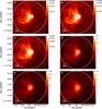 |
Fig. B.31 Same image layout as Fig. B.1 but for ISOSS J06114+1726. |
| In the text | |
|
Fig. B.32 Same image layout as Fig. B.1 but for ISOSS J06527+0140. Cyan contours on the SPIRE panels d)–f) show SCUBA 850 μm: 0.41, 0.62, 0.82, 1.03, 1.24, 1.44, 1.65, 1.85, 2.06 Jy beam-1. |
| In the text | |
|
Fig. B.33 Same image layout as Fig. B.1 but for ISOSS J18364-0221. Cyan contours on the SPIRE panels d)–f) show SCUBA 850 μm: 0.21, 0.31, 0.42, 0.52, 0.63, 0.73, 0.83, 0.94, 1.04 Jy beam-1. |
| In the text | |
|
Fig. B.34 Same image layout as Fig. B.1 but for ISOSS J19357+1950. Cyan contours on the SPIRE panels d)–f) show SCUBA 850 μm: 0.06, 0.09, 0.12, 0.15, 0.17, 0.20, 0.23, 0.26, 0.29 Jy beam-1. |
| In the text | |
|
Fig. B.35 Same image layout as Fig. B.1 but for ISOSS J19486+2556. Cyan contours on the SPIRE panels d)–f) show SCUBA 850 μm: 0.07, 0.11, 0.14, 0.18, 0.22, 0.25, 0.29, 0.32, 0.36 Jy beam-1. |
| In the text | |
|
Fig. B.36 Same image layout as Fig. B.1 but for ISOSS J19557+2825. Cyan contours on the SPIRE panels d)–f) show SCUBA 850 μm: 0.13, 0.19, 0.26, 0.32, 0.38, 0.45, 0.51, 0.58, 0.64 Jy beam-1. |
| In the text | |
|
Fig. B.37 Same image layout as Fig. B.1 but for ISOSS J20093+2729. Cyan contours on the SPIRE panels d)–f) show SCUBA 850 μm: 0.05, 0.08, 0.10, 0.13, 0.15, 0.18, 0.20, 0.23, 0.25 Jy beam-1. |
| In the text | |
|
Fig. B.38 Same image layout as Fig. B.1 but for ISOSS J20153+3453. Cyan contours on the SPIRE panels d)–f) show SCUBA 850 μm: 0.28, 0.41, 0.55, 0.69, 0.83, 0.97, 1.10, 1.24, 1.38 Jy beam-1. |
| In the text | |
|
Fig. B.39 Same image layout as Fig. B.1 but for ISOSS J20298+3559. Cyan contours on the SPIRE panels d)–f) show SCUBA 850 μm: 0.08, 0.12, 0.20, 0.24, 0.28, 0.32, 0.36, 0.40 Jy beam-1. |
| In the text | |
|
Fig. B.40 Same image layout as Fig. B.1 but for ISOSS J21311+5127. Cyan contours on the SPIRE panels d)–f) show SCUBA 850 μm: 0.12, 0.18, 0.24, 0.30, 0.36, 0.42, 0.48, 0.54, 0.60 Jy beam-1. |
| In the text | |
|
Fig. B.41 Same image layout as Fig. B.1 but for ISOSS J22164+6003. Cyan contours on the SPIRE panels d)–f) show SCUBA 850 μm: 0.08, 0.12, 0.20, 0.24, 0.28, 0.32, 0.36, 0.40 Jy beam-1. |
| In the text | |
|
Fig. B.42 Same image layout as Fig. B.1 but for ISOSS J22478+6357. Cyan contours on the SPIRE panels d)–f) show SCUBA 850 μm: 0.11, 0.17, 0.22, 0.28, 0.34, 0.39, 0.45, 0.50, 0.56 Jy beam-1. |
| In the text | |
|
Fig. B.43 Same image layout as Fig. B.1 but for ISOSS J23053+5953. Cyan contours on the SPIRE panels d)–f) show SCUBA 850 μm: 0.4, 0.6, 0.8, 1.0, 1.2, 1.4, 1.6, 1.8, 2.0 Jy beam-1. |
| In the text | |
|
Fig. B.44 Same image layout as Fig. B.1 but for ISOSS J23129+5944. Cyan contours on the SPIRE panels d)–f) show SCUBA 850 μm: 0.14, 0.21, 0.28, 0.35, 0.42, 0.49, 0.56, 0.63, 0.70 Jy beam-1. |
| In the text | |
|
Fig. B.45 Same image layout as Fig. B.1 but for ISOSS J23287+6039. Cyan contours on the SPIRE panels d)–f) show SCUBA 850 μm: 0.08, 0.12, 0.20, 0.24, 0.28, 0.32, 0.36, 0.40 Jy beam-1. |
| In the text | |
Current usage metrics show cumulative count of Article Views (full-text article views including HTML views, PDF and ePub downloads, according to the available data) and Abstracts Views on Vision4Press platform.
Data correspond to usage on the plateform after 2015. The current usage metrics is available 48-96 hours after online publication and is updated daily on week days.
Initial download of the metrics may take a while.