| Issue |
A&A
Volume 540, April 2012
|
|
|---|---|---|
| Article Number | A84 | |
| Number of page(s) | 23 | |
| Section | Interstellar and circumstellar matter | |
| DOI | https://doi.org/10.1051/0004-6361/201117914 | |
| Published online | 30 March 2012 | |
Water in star-forming regions with Herschel: highly excited molecular emission from the NGC 1333 IRAS 4B outflow ⋆,⋆⋆
1 Max-Planck-Institut für extraterrestriche Physik, Postfach 1312, 85741 Garching, Germany
e-mail: This email address is being protected from spambots. You need JavaScript enabled to view it.
2 Kavli Institute for Astronomy and Astrophysics, Peking University, Beijing 100871, PR China
3 Sterrewacht Leiden, Leiden University, PO Box 9513, 2300 RA Leiden, The Netherlands
4 Niels Bohr Institute and Centre for Star and Planet Formation, University of Copenhagen, Juliane Maries Vej 30, 2100 Copenhagen Ø., Denmark
5 Department of Astronomy, The University of Michigan, 500 Church Street, Ann Arbor, MI 48109-1042, USA
6 Institute for Astronomy, ETH Zurich, 8093 Zurich, Switzerland
7 Space Telescope Science Institute, 3700 San Martin Drive, Baltimore, MD 21218, USA
Received: 18 August 2011
Accepted: 17 January 2012
Abstract
During the embedded phase of pre-main sequence stellar evolution, a disk forms from the dense envelope while an accretion-driven outflow carves out a cavity within the envelope. Highly excited (E′ = 1000 − 3000 K) H2O emission in spatially unresolved Spitzer/IRS spectra of a low-mass Class 0 object, NGC 1333 IRAS 4B, has previously been attributed to the envelope-disk accretion shock. However, the highly excited H2O emission could instead be produced in an outflow. As part of the survey of low-mass sources in the Water in Star Forming Regions with Herschel (WISH-LM) program, we used Herschel/PACS to obtain a far-IR spectrum and several Nyquist-sampled spectral images to determine the origin of excited H2O emission from NGC 1333 IRAS 4B. The spectrum has high signal-to-noise in a rich forest of H2O, CO, and OH lines, providing a near-complete census of far-IR molecular emission from a Class 0 protostar. The excitation diagrams for the three molecules all require fits with two excitation temperatures. The highly excited component of H2O emission is characterized by subthermal excitation of ~1500 K gas with a density of ~3 × 106 cm-3, conditions that also reproduce the mid-IR H2O emission detected by Spitzer. On the other hand, a high density, low temperature gas can reproduce the H2O spectrum observed by Spitzer but underpredicts the H2O lines seen by Herschel. Nyquist-sampled spectral maps of several lines show two spatial components of H2O emission, one centered at ~5′′ (1200 AU) south of the central source at the position of the blueshifted outflow lobe and a heavily extincted component centered on-source. The redshifted outflow lobe is likely completely obscured, even in the far-IR, by the optically thick envelope. Both spatial components of the far-IR H2O emission are consistent with emission from the outflow. In the blueshifted outflow lobe over 90% of the gas-phase O is molecular, with H2O twice as abundant than CO and 10 times more abundant than OH. The gas cooling from the IRAS 4B envelope cavity walls is dominated by far-IR H2O emission, in contrast to stronger [O I] and CO cooling from more evolved protostars. The high H2O luminosity may indicate that the shock-heated outflow is shielded from UV radiation produced by the star and at the bow shock.
Key words: infrared: ISM / ISM: jets and outflows / stars: protostars / molecular processes / stars: individual: NGC 1333 IRAS 4B
Herschel is an ESA space observatory with science instruments provided by European-led Principal Investigator consortia and with important participation from NASA.
Appendices are only available in electronic form at http://www.aanda.org
© ESO, 2012
1. Introduction
During the embedded phase of pre-main sequence stellar evolution, the protoplanetary disk forms out of a dense molecular envelope (e.g. Terebey et al. 1984; Adams et al. 1987). Meanwhile, as the protostar builds up most of its mass, it drives powerful, collimated outflows into the dense envelope (e.g. Bontemps et al. 1996). These processes together eventually cause the envelope to dissipate and set the initial conditions for disk evolution and planet formation.
At the interfaces between the outflow and envelope and between envelope and disk, shocks can heat the gas and potentially produce detectable emission. The well-studied outflow-envelope interactions produce an outflow cavity with walls heated by shocks and energetic radiation from the central star (e.g. Snell et al. 1980; Spaans et al. 1995; Arce & Sargent 2006; van Kempen et al. 2009; Tobin et al. 2010). On the other hand, observational evidence for the disk-envelope interactions has been sparse. Velusamy et al. (2002) detected methanol emission from L1157 on scales of ~1000 AU, spatially-extended beyond the point-like continuum emission, and argued that the kinematics suggest that the emission is produced at the disk/envelope interface. Watson et al. (2007) detected emission in highly excited (E′ = 1000 − 3000 K) H2O lines from the NGC 1333 IRAS 4B system and attributed the heating to an envelope-disk accretion shock within 100 AU of the star. These observations offer two different interpretations for disk-envelope interactions, with material either entering the disk on large scales (Visser et al. 2009; Vorobyov 2011) or raining onto the disk at small radii (Whitney & Hartmann 1993). However, a persistent complication in interpreting spatially and spectrally unresolved emission as coming from a compact disk-like structure is that outflows can also produce bright emission in highly excited lines. Molecular emission is a dominant coolant of outflow-envelope interactions, and H2O emission is particularly sensitive to shocks in outflows (e.g. Nisini et al. 2002, 2010; van Kempen et al. 2010a).
The NGC 1333 IRAS 4B system (hereafter IRAS 4B) is a Class 0 YSO (d = 235 pc, Hirota et al. 2008) with a 0.24 M⊙ disk that is deeply embedded (AV ~ 1000 mag) within a 2.9 M⊙ envelope (Jørgensen et al. 2002, 2009). Compact outflow emission is detected in many sub-millimeter (sub-mm) molecular lines (Di Francesco et al. 2001; Jørgensen et al. 2007). Near-IR emission in all four Spitzer/IRAC bands (3.5, 4.5, 5.8, and 8.0 μm) is located in the blueshifted outflow lobe (Jørgensen et al. 2006, see also Choi et al. 2011), offset by ~6′′ south of the peak of interferometric sub-mm continuum emission. The redshifted outflow is seen in sub-mm line emission (Jørgensen et al. 2007) but is not detected in the near- or mid-IR because the outflow is located behind IRAS 4B and hidden by the high extinction of the envelope.In the near-IR, the Spitzer/IRAC photometry is dominated by H2 emission (Arnold et al. 2011; see also Neufeld et al. 2008), with some contribution of CO fundamental emission to the 4.5 μm bandpass (Tappe et al. 2011; see also Herczeg et al. 2011). Excited water emission from the NGC 1333 IRAS 4 system, including both IRAS 4A and 4B, was detected with ISO/LWS, but with too low spatial resolution to attribute the emission to any component in the system (Giannini et al. 2001). H2O maser emission has also been seen from dense gas associated with the IRAS 4B outflow, although with a different position angle than the molecular outflow (Rodriguez et al. 2002; Furuya et al. 2003; Marvel et al. 2008; Desmurs et al. 2009).
In a sample of low-resolution Spitzer-/IRS spectra of 30 Class 0 objects, Watson et al. (2007) found water emission from highly-excited levels in only IRAS 4B. The lines have upper levels with high excitations (1000−3000 K) and high critical densities (~1011 cm-3). Watson et al. inferred that the emitting gas has a high density and argued that the high density indicates that the emission is produced in a ~2 km s-1 accretion shock at the envelope-disk interface. They also argued that the emission was detected only from IRAS 4B because the viewing angle may be well-aligned with the outflow, allowing a clear view of the embedded disk, and because the timescale for such high envelope-disk accretion rates may be short. H2O emission has since been detected in at least two other components of the IRAS 4B system: (1) narrow (~1 km s-1, with rotation signatures) p-H O 313 − 220 (E′ = 204 K) emission in a spatially compact region, likely a (pseudo)-disk of ~25 AU in radius (Jørgensen & van Dishoeck 2010); and (2) broad (FWHM ~ 24 km s-1), spatially unresolved emission from low-excitation H2O (E′ = 50−250 K) lines, which are consistent with an outflow origin (Kristensen et al. 2010) but too broad for the ~2 km s-1 velocity expected of envelope gas in free-fall striking the disk at 25–100 AU (e.g. Shu et al. 1977).
The highly-excited mid-IR emission and the broad line profiles of lower-excitation lines could be reconciled if either (a) the high- and low-excitation H2O emission lines originate in different locations, if (b) models for the envelope-disk accretion shock underpredict line widths, or if (c) both the high- and low-excitation H2O lines are produced in the outflow. In this paper, we analyze a Herschel/PACS far-IR spectral survey and spectral imaging of IRAS 4B to resolve the discrepancy in the different possible origins of H2O emission from IRAS 4B. The far-IR spectrum of IRAS 4B is as rich in lines as its mid-IR Spitzer/IRS spectrum. In Nyquist-sampled maps, the H2O emission is spatially offset from the continuum emission in the direction of the blueshifted outflow. The excitation of warm H2O lines detected with Herschel/PACS and with Spitzer/IRS together can be explained by emission from an isothermal slab. An additional physical component(s) is located on-source and likely traces material closer to the base of the outflow.No evidence is seen for an envelope-disk accretion shock. This result is consistent with a conclusion by Tappe et al. (2012), obtained contemporaneous to the results in this paper, that the H2O emission seen in the Spitzer/IRS spectra also coincides with the southern outflow position. We discuss the implications of these results for outflows and for the prospects of observationally studying disk formation with H2O lines.
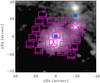 |
Fig. 1 The location of the 5 × 5 spaxel array (purple spectral map) against an 4.5 μm image obtained with Spitzer/IRAC (grayscale) from Jørgensen et al. (2006). The spectral map shows that the continuum-subtracted emission in the o-H2O 616−505 82.03 μm (E′ = 643 K) line is produced mostly in the blueshifted outflow lobe. The sub-mm positions of IRAS 4B and IRAS 4A are marked with blue asterisks. |
2. Observations and data reduction
We obtained far-IR spectra of NGC 1333 IRAS 4B (03h29m12 0 +31°13′08
 1; Jørgensen et al. 2007) on 15–16 March 2011 with the PACS instrument on Herschel (Pilbratt et al. 2010; Poglitsch et al. 2010) as part of the WISH key program (van Dishoeck et al. 2011). The observations presented here consist of a complete scan of the 52–208 μm spectral range and deep, Nyquist-sampled spectral maps in four narrow (~0.5 − 1 μm) wavelength regions. Each PACS spectrum includes observations of two different nod positions located at ± 3′ from the science observation to subtract the instrumental background. All PACS data were reduced with HIPEv6.1 (Ott 2010). We supplemented the PACS observations with re-reduced archival Spitzer/IRS spectra that were previously analyzed by Watson et al. (2007). Details of the observations and reduction are described in the following subsections.
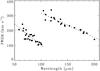 |
Fig. 2 The FWHM from initial fits to strong lines in our full scan of the 52–208 μm wavelength range. The lines are spectrally unresolved and provide a measure of the spectral resolution. The line widths for our final fits were set by linear fits to the FWHM at > 100 and < 100 μm. |
2.1. Complete Herschel/PACS far-IR spectrum
The 52–208 μm spectrum of IRAS 4B was obtained in 2.7 h of integration with PACS. PACS observed IRAS 4B simultaneously in the first order >100 μm and in the second order at < 100 μm. The grating resolution varies between R = 1000−2000 at > 100 μm and R = 3000−4000 at <100 μm. Large grating steps are used, so the spectrum is binned to ~2 pixels per resolution element. A spectral flatfielding was applied to the data to improve the S/N. The observed flux was normalized to the telescopic background and subsequently calibrated from observations of Neptune, which is used as a spectral standard.Appendix A describes a new method to calibrate the flux in PACS spectra between 97–103 μm and above >190 μm. The relative flux calibration is accurate to ~20% acrossmost of the spectrum.
The spectral scan produced a single 5 × 5 spectral map over a 47′′ × 47′′ field-of-view. The central spaxel is centered at the location of the sub-mm continuum peak. An adjacent spaxel located  to the SE (PA = 249°) is centered on the blueshifted outflow position (Fig. 1). Most of the line and continuum flux is located in these two spaxels. The southern outflow of NGC 1333 IRAS 4A is located in the NW corner of the array.
Extracting line fluxes requires an assessment of the distribution of flux on the detector caused by both the point-spread function of Herschel and the spatial extent of the emission. For a well-centered point source, the encircled energy in a single spaxel is ~70% at ≤100 μm wavelengths and declines to ~40% near 200 μm. However, the signal-to-noise decreases if the spectrum is extracted from many spaxels. The emission line spectrum is obtained by adding the flux from the central spaxel and the outflow spaxel. The line fluxes are subequently corrected for light leakage and the spatial extent in the emission by comparing line fluxes from this 2-spaxel extraction with the line fluxes extracted from a 3 × 3 spaxel area centered on the central spaxel. The line flux ratio between the 2-spaxel and 3 × 3 spaxel extraction was calculated for strong lines of all detected molecules. The fluxes from the 2-spaxel extraction are then divided by a wavelength-dependent correction that is 0.76 at <100 μm and then decreases linearly to 0.6 at 180 μm. The wavelength dependence of this correction includes both the point-spread function of Herschel and the wavelength dependence in the spatial distribution of the detected emission. Finally, high signal-to-noise PACS spectra of the point source HD 100546 (Sturm et al. 2010) were then used to correct for emission leaked beyond the 3 × 3 spaxel area. This approach assumes a similar spatial distribution for all molecules and for lines at nearby wavelengths, and introduces a ~10% uncertainty in relative fluxes. The overall uncertainty in flux calibration is ~30%. The typical noise level in the two-spaxel extraction (~9.4 × 18.8′′) is ~0.4 Jy per resolution element in the extracted continuum spectrum.
Location of PACS line and continuum emission from the IRAS 4B system.
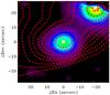 |
Fig. 3 The 63 μm continuum emission (colors) and the SCUBA 450 μm emission map (contours), with the location of IRAS 4A and IRAS 4B marked as white asterisks. The PACS maps are shifted so that the centroid of the 190 μm continuum emission is located at the position of IRAS 4B obtained from sub-mm continuum interferometry. The SCUBA map is shifted to the same position. |
All lines in the complete spectral scan are spectrally unresolved.The lines were initially fit with Gaussian profiles, with the central wavelength, line width, and amplitude and a first-order continuum as free parameters. The instrumental line widths were then calculated from first-order fits to the wavelength-dependent spectral resolution, obtained from strong lines (Fig. 2). Our final fluxes are obtained from fitting Gaussian profiles to each line, with the line width set by the calculated instrumental resolution at the given wavelength. For strong lines, the median centroid velocity is 30 km s-1 with a standard deviation of 24 km s-1. The absolute wavelength calibration is accurate to ~50 km s-1 and is limited by the spatial distribution of emission within each spaxel.
2.2. Herschel/PACS Nyquist-sampled spectral imaging
Nyquist-sampled spectral maps of narrow spectral regions at 54.5, 63.3, 108.5, and 190 μm were obtained in a total of 2.2 h of integration time. These maps were obtained from a 3 × 3 raster scan with 3′′ steps, yielding spatial resolutions of ~5′′, 5′′, 8′′, and 10′′, respectively. Small grating steps were used to fully sample the spectral resolution. The final spectrum is rebinned onto a wavelength grid with ~4 pixels per resolution element.
The spectral maps include CO, H2O, and [O I] lines listed in Table 1. In a 3 × 3′′ area, the typical rms is ~0.02 Jy per resolution element at 63 μm and ~0.01 Jy per resolution element at 108 μm. This sensitivity level is better than that from the full spectral scan because of different integration areas and much longer integration times in each resolution element.
The data cubes from the Nyquist-sampled maps were reprojected onto a normal grid of right ascension and declination. In the automated calibration the 190 μm continuum emission is offset from the object position1, as measured from sub-mm interferometry (Jørgensen et al. 2007). Each map is shifted in position by  E and
E and  N so that the location of the 190 μm continuum from our observations matches the peak location of the sub-mm emission. After the shift, the 63 and 108 μm continuum emission from IRAS 4B and IRAS 4A (located in the NW edge of the map) are well aligned with the Spitzer-MIPS 70 μm emission. No significant offset was measured in the staring observation of the full PACS SED, which was obtained with a new pointing one day after the Nyquist-sampled map. Because the same spatial shift is applied to both the line and far-IR continuum emission maps and because the shift moved both the line and continuum closer to the sub-mm continuum peak, the result that the line emission is spatially offset from the sub-mm continuum is robust to the pointing uncertainty.
The southern nod position in the map has spatially-extended [O I] emission in the southwest portion of the map. The [O I] emission is therefore measured from only the northern nod position. Inspection of Spitzer/MIPS 70 μm maps at the two nod positions does not indicate the presence of a strong, point-source continuum emission that could otherwise corrupt the continuum map for IRAS 4B.The 54 μm continuum map has low S/N and is not used.
The two H2O and [O I] lines at 63 μm have spectral widths of 110 km s-1, which places an upper limit of 65 km s-1 on the intrinsic line width. That the line widths are broader than the instrumental resolution of ~3300 is not significant because emission that is spatially extended in the cross-dispersion direction can broaden the spectral line profile, as with any other slit spectrograph.
2.3. Spitzer/IRS spectrum
The Spitzer/IRS spectra of IRAS 4B were originally presented by Watson et al. (2007). We re-reduced the spectrum following the procedure described by Pontoppidan et al. (2010). The LH slit width is 11′′. The flux extraction region of 5–10′′ across the wavelength region was selected to optimize the final signal-to-noise in the limit of a point source (Horne 1986). The Spitzer and Herschel observations cover similar regions on the sky. The relative flux calibration between Spitzer and Herschel spectra is likely uncertain by ~30% flux.
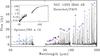 |
Fig. 4 The combined Herschel/PACS and Spitzer/IRS continuum-subtracted spectra of IRAS 4B, with bright emission in many H2O (blue marks), CO (red marks), OH (green marks), and atomic or ionized lines (purple). The Spitzer spectrum is multiplied by a factor of 10 so that the lines are strong enough to be seen on the plot. The inset shows the combined spectrum including the continuum. |
3. Results
3.1. Far-IR spectrum of IRAS 4B
The far-IR PACS spectrum of IRAS 4B is the richest far-IR spectrum of a YSO to date. A forest of high signal-to-noise CO, H2O, and OH lines that provide a full census of far-IR molecular emission that can be detected from low-mass YSOs (Fig. 4; see also Figs. D.1, D.2 in the Appendix). Lines were discovered in the spectrum following a biased search for emission at the wavelengths for transitions of common species and an unbiased search for narrow features that peak above the noise level.
A total of 115 distinct emission lines are detected and identified from IRAS 4B (Table 3). All strong lines are identified. Several tentative detections of weak lines are unidentified and discussed in Appendix B. No HO or 13CO emission is detected in the PACS observations, with typical flux limits in the strongest expected lines of ~0.03 times the observed flux of the main isotopologue. The [O I] 145.5 μm line is not detected, with a 2σ flux limit 1.2 × 10⁻²¹ W cm-2. Lines of OH+ and CH+, HD 56 and 112 μm, [N II] 121.8 and 205.2 μm, [C II] 157.7 μm, and [O III] 88.7 μm are also not detected.
Figure 1 shows a spectral map of the o-H2O 616 − 505 82.03 μm (E′ = 643 K) line emission overplotted on a Spitzer/IRAC 4.5 μm image of IRAS 4B (and IRAS 4A). The line emission is located at the position of the near-IR emission in the blueshifted outflow lobe, south of the central source of IRAS 4B. On the other hand, most of the continuum emission is located in the central spaxel, consistent with the location of the sub-mm continuum emission. Figure 5 demonstrates that the equivalent width of far-IR lines is much larger in the outflow spaxel than in the continuum spaxel, indicating a spatial offset between the line and continuum emission. The line emission in the central spaxel mostly disappears at <70 μm. All lines in the PACS spectrum are spatially offset from the continuum emission. The line fluxes are measured based on the summation of these two bright spaxels and correction for spatial extent (see Sect. 2.1).
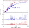 |
Fig. 5 Top: spectra extracted separately from a spaxel centered on the sub-mm continuum (red) and a spaxel offset by |
3.2. PACS mapping of H2O Emission from IRAS 4B
Figure 6 and Table 1 compare the spatial distribution of the continuum flux with H2O, CO, and [O I] line fluxes obtained from the Nyquist-sampled spectral maps. The far-IR continuum emission is centered on-source, at the location of the sub-mm continuum, while line emission is centered to the south in the blueshifted outflow. Figure 7 shows a cartoon version of the approximate location of line and continuum emission and the morphology of IRAS 4B. In the following analysis, we simplify the analysis by assuming that emission consists of two unresolved point sources, one at the outflow position and one at the sub-mm continuum peak, and are subsequently fit with 2D Gaussian profiles. More complicated spatial distributions would be unresolved in our maps.
The right panel of Fig. 6 demonstrates that the location of the warm H2O coincides with the Spitzer/IRAC 4.5 μm imaging. The two H2O lines near 63.4 μm, o-H2O 818−707 and p-H2O 808−717, (E′ = 1070 K) are centered at 5.2 ± 0.2′′ from the 63 μm continuum and are spatially extended relative to the continuum emission (assumed to be unresolved for simplicity) by FWHM = 6.7 ± 1.0′′. About 70% of the emission is produced at the southern outflow position (Fig. 8). The flux ratios for the two H2O 63.4 μm lines are similar at both the on-source and off-source positions (Fig. 9). In the 108.5 μm spectral map, both the o-H2O 221 − 110 (E′ = 194 K) and CO 24–23 (E′ = 1524 K) emission are centered 2.5 ± 0.4′′ south of the 108.5 μm continuum emission and are spatially-extended in the outflow direction by 13.6 ± 0.7′′, relative to the extent of the continuum emission. The larger spatial extent and smaller offset in the 108 μm lines both indicate that the outflow component contributes ~40% of the measured line flux. The spatial differences may be interpreted as differential extinction across the emission region, discussed in the next subsection.
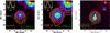 |
Fig. 6 Left and Middle: contour maps of H2O (yellow), [O I] (red, left), and CO (red, middle) emission compared with continuum emission (color contours) at 63.3 μm (left) and 108.5 μm (middle). The insets show the spatial extent of continuum and line emission in the different components along the N-S outflow axis. Right: a comparison of the location of emission in H2O 63.32 μm (blue), 108.5 μm continuum (red), Spitzer-IRAC 4.5 μm photometry (color contours; Jørgensen et al. 2006; Gutermuth et al. 2008). All contours have levels of 0.1,0.2,0.4,0.8, and 1.6 times the peak flux near IRAS 4B. The asterisks show the sub-mm positions of IRAS 4B near the center of the field and IRAS 4A in the NW corner. Some noise in these maps is suppressed at empty locations far from IRAS 4A and IRAS 4B. |
The 54 μm maps are noisy because PACS has poor sensitivity at <60 μm. The o-H2O 532−505 54.507 μm (E′ = 732 K) emission is offset by 5.9 ± 0.4′′ south from the the peak of the sub-mm continuum emission. The CO 49-48 53.9 μm emission (E′ = 6457 K) is offset 2.9 ± 0.4′′ south, between the peak of the sub-mm emission and the bright outflow location. The highly-excited CO emission is produced in a different location than the highly-excited H2O emission.
The [O I] emission is offset by 3.7 ± 0.3′′ at PA = 168°, just west of the outflow, and is spatially extended by ~  .
.
3.3. Extinction estimates to the central source and outflow position
The extinction to different physical structures within the IRAS 4B system depends on how much envelope material is present in our line of sight. In this subsection, we discuss how these different extinctions affects the emission that is seen. The extinction law used here is obtained from Weingartner & Draine (2001) with a total-to-selective extinction parameter RV = 5.5, typical of dense regions in molecular clouds (e.g. Indebetouw et al. 2005; Chapman et al. 2009). Appendix D includes a discussion of how extinctions may affect the molecular excitation diagrams.
The strength of the near-IR emission in the outflow (Jørgensen et al. 2006) indicates that extinction must be low to at least some of the outflow position. Spherical models of the dust continuum indicate that the central protostar is surrounded by AV = 1000 mag (Jørgensen et al. 2002), so any emission from the redshifted outflow lobe may suffer from as much as AV ~ 2000 mag of extinction. Any additional extinction would have likely introduced asymmetries in the H2O line profiles that were presented in Kristensen et al. (2010). Depending on the wavelength and spatial location of the emission, the far-IR emission line fluxes may be severely affected by extinction.
The H2O 54.5 and 63.4 μm lines have a different spatial distribution than the H2O 108.1 μm line. If we assume that the on-source and off-source emission both have similar physical conditions, then the ratio of the H2O 63.4 to 108.1 μm line luminosities should not change with position. In this scenario, the different locations for the detected flux is caused by differential extinction across the emission area. An average extinction to the on-source H2O component of AV ~ 700 mag would reduce the fractional contributions from the on-source and off-source locations observed values. This extinction may be the combination of a lightly-extincted region on the front side of the protostar and a heavily-extincted region on the back side of the protostar.
An independent estimate of the extinction can also be made from the flux ratio of [O I] 63.18 to 145.5 μm lines, which is typically observed to be about 10 (Giannini et al. 2001; Liseau et al. 2006). The undetected [O I] 145.5 μm line flux is less than 10% of the 1.8 × 10⁻²⁰ W cm-2 flux in the [O I] 63.18 μm line. If we conservatively assume that the true ratio is 30, then we estimate AV < 200 mag to the [O I] emission region. Some additional [O I] emission could only be hidden behind a high enough extinction (AV ~ 4000 mag) to attenuate emission in both the 63.18 and 145.5 μm lines. Therefore, the effect of extinction on the [O I] luminosity is likely not too significant for the southern outflow lobe, where [O I] emission is seen.
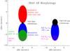 |
Fig. 7 A cartoon showing the location of different emission components from IRAS 4B, based in part on Fig. 6. |
3.4. Spitzer/IRS spectrum and broadband images of IRAS 4B
The Spitzer/IRS spectrum of IRAS 4B includes emission in lines of highly-excited H2O and OH, plus [S I] and [Si II]. Our line identification mostly agrees with that of Watson et al. (2007) for H2O lines, with some modifications to account for the identifications of OH lines (Table 2 and Fig. 10, see also Tappe et al. 2008). The H2O line identification was informed from line intensities predicted by RADEX modelling (see Sect. 4.1) of both the low-density case discussed here and the high density-case of Watson et al. (2007). All lines with significant detections are identified.
An analysis of the Spitzer/MIPS 24 μm image, with sensitivity from 20–31 μm, helps us place limits on the amount of H2O emission that could arise on-source. Convolving the filter transmission curve with the Spitzer/IRS spectrum from Watson et al. (2007) indicates that ~24% of the light in the MIPS 24 μm bandpass is in molecular emission (mostly H2O), 17% in the [S I] 25.24 μm line, and 59% in the continuum.
Jørgensen & van Dishoeck (2010) found that the emission from IRAS 4B in the Spitzer/MIPS 24 μm images is offset from the peak emission of the sub-mm continuum (see also Choi & Lee 2011). We measure that the emission is centered at  S and
S and  E from the central source, consistent with the location of the outflow emission, and is spatially extended by ~
 in the north-south direction, along the outflow axis. An additional component is present at the location of the sub-mm continuum peak. The Spitzer/MIPS emission is assumed here to be a combination of emission from two unresolved sources, one at the sub-mm continuum peak and one at the position of the Spitzer IRAC 4.5 μm emission located 62 S and 04 E. From fitting two dimensional Gaussian profiles to the image, the component at the blueshifted outflow lobe accounts for 78% of the Spitzer/MIPS 24 μm emission and the sub-mm point source accounts for the remaining 22% of the emission (see Fig. 8 for the fit to the image collapsed onto the outflow direction). Some additional Spitzer/MIPS emission is located at 20′′ S of the sub-mm continuum peak and is ignored here.
In the Spitzer/IRAC images of emission between 3.8–8 μm, the emission is located entirely at the outflow position. In contrast, the 63 μm continuum emission is located mostly on the central source at the sub-mm continuum position. Much of the 20–31 μm continuum emission must be located at the outflow position, but some continuum emission could also be located on the central source. Given the fraction of emission located on-source (22%) and the relative contributions of molecular lines (24%) and continuum to the Spitzer/MIPS photometry, the MIPS map could be consistent with an on-source location of H2O emission only if the continuum emission is located entirely at the outflow position.
4. Excitation of molecular emission from IRAS 4B
The spatial distribution of the highly excited H2O emission in the PACS observations places the bulk of the highly excited far-IR emission at the outflow position. In this section, we analyze the excitation of the H2O lines in detail to demonstrate that the highly excited H2O emission in both the Herschel/PACS and Spitzer/IRS spectra can be explained with emission from a single isothermal, plane-parallel slab. We subsequently analyze CO, OH, and [O I] emission from IRAS 4B. Although the H2O emission region is likely complicated and includes multiple spatial and excitation temperature components, our simplified approach is able to reproduce the highly excited H2O lines. The properties of this slab are the combination of the spatially offset outflow component and the on-source component. We lack sufficient spatial resolution throughout most of the spectrum to analyze the excitation of the two components separately.
Figure 11 shows excitation diagrams for H2O, CO, and OH emission2. Without considering sub-thermal excitation, each molecule requires two temperature components to reproduce the measured fluxes. For convenience, the two components for each molecule are called “warm” and “cool”, however this terminology applies separately to each molecule3. The warmer component of CO may not be related to the warmer component of H2O or OH. For the temperature and density derived below, the two apparent excitation temperatures for OH and H2O could even be produced by a single component, with the warm and cool regimes resulting from subthermal excitation. Table 3 describes the excitation temperatures, molecular column density, and luminosity for fits to these diagrams. In the following subsections we discuss the excitation of the H2O in detail, and briefly describe the excitation of CO, OH, and O. RADEX models of H2O are used to fit only the higher excitation H2O lines because the lower excitation lines are optically thick and difficult to use to infer physical conditions of the emitting gas. The emitting area, temperature, and density derived from the fits to the observed H2O lines are assumed to also apply to CO, OH, and O for simplicity.
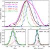 |
Fig. 8 Top: a cross cut of the flux at several wavelengths along the N-S outflow axis. The 63 μm continuum is centered at the peak of the sub-mm continuum while the 4.5 μm and 24 μm photometry are centered in the outflow. The H2O 63.3 μm lines are produced primarily at the outflow location while the H2O 108.1 μm line has similar on- and off-source contributions. The (0,0) position is defined here by the peak of the sub-mm continuum emission from Jørgensen et al. (2007). Bottom: the spatial cross cut of H2O 63.3 μm and MIPS 24 μm emission, shown as the combination of two unresolved Gaussian profiles located at the on-source position (red dashed line) and the blueshifted outflow position (blue dashed line). |
4.1. RADEX models of H2O emission
The H2O line emission extends to high energy levels, with level populations indicating an excitation temperature of 220 K but with significant scatter. Among the highly excited lines, the H2O excitation diagram does not show any break at high energies that would indicate multiple excitation components. The highly-excited H2O levels have high critical densities (~1011 cm-3). The bottom left panel in Fig. 11 demonstrates that a large amount of scatter in excitation diagrams may be explained by sub-thermal excitation. The excitation temperature could therefore be the kinetic temperature of dense (>1011 cm-3) gas or could result from subthermal excitation of warmer gas with lower density. Line opacities also increase the scatter in observed fluxes.
We calculate synthetic H2O spectra from RADEX4 models of a plane-parallel slab (van der Tak et al. 2007) characterized by a single temperature T, density n(H2), and H2O column density N(H2O) with an emitting surface area A. RADEX is a radiative transfer code that simultaneously calculates non-LTE level populations and line optical depths for a plane-parallel slab to produce line fluxes. A large grid was calculated using molecular data obtained from LAMDA (Schöier et al. 2005; Faure et al. 2007). Since this molecular data file lacks the most highly excited lines detected with Spitzer, individual RADEX models were calculated at specific gridpoints using a much larger and more complete database with energy levels obtained from Tennyson et al. (2001), radiative rates from the HITRAN database (Rothman et al. 2009), and collisional rates with H2 from Faure et al. (2008).
The RADEX models are calculated to obtain a rough idea of the physical properties of the emitting gas. Radiative pumping is not included in the model but is likely important, especially at low densities. Including radiative pumping would require detailed physical and chemical modeling of the envelope and is beyond the scope of this work. The line profile is assumed to be a Gaussian profile with a FWHM of 25 km s-1, based on the FWHM of low-excitation H2O lines observed with HIFI (Kristensen et al. 2010)5. The extinction to the warm H2O gas is highly uncertain and is mostly ignored (see Sect. 3.3 and Appendix D for a discussion of extinction estimates and their implications). The ortho-to-para ratio is assumed to be 3, based on flux ratios of optically-thin lines that range from 2.8–3.5.
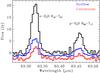 |
Fig. 9 The H2O 63.4 μm spectral region extracted from the on-source position (red) and from the blueshifted outflow position (blue), and over the entire spectral map (black). No significant differences are detected in the ratio of the two lines, which indicate that the two lines are optically thin at both locations. |
A χ2 fit (upper left panel of Fig. 12) to the measured fluxes with PACS and IRS lines with upper energy level above 400 K (the warm component) yields acceptable solutions with high temperature (T > 1000 K) and H2 densities of log n < 7.5. Appendix C provides a detailed description of the line ratios and the non-detections of HO emission that constrain the best-fit parameters. The size of the emission region further limits the range of acceptable parameter space (Fig. 12). The emitting surface area A is equivalent to the area of a circle with radius from 25–500 AU, which is reasonably close to the projected length of the outflow on the sky (~1000 AU or 0.005 pc). If we assume that N(H2O) < 10-4N(H2), then the given column density and H2 density yields the length scales (depth along our line of sight) for the outflow that range from >10-4 pc (for the acceptable model with the highest H2 density and lowest H2O column density) to > 130 pc (for the model with the lowest H2 density and highest H2O column density). Given the projected size of the outflow of 0.005 pc, a length scale greater than 0.1 pc is uncomfortably large and rules out solutions with log n(H2) < 5. The lack of obvious vibrational excitation in spectra at 6 μm (Maret et al. 2009; Arnold et al. 2011) limits the kinetic temperature to ≲ 2000 K. The number of H2O molecules scales with density.
Combining these analyses, we adopt the parameters  K, log n = 6.5 ± 1.5, and log N(H2O) = 17.6 ± 1.2 over an emitting area equivalent to a circle with radius 25−300 AU and length scale 0.003 pc. Figure 13 shows that the PACS H2O spectrum is well fit with model fluxes obtained with these parameters.
The temperature and column density are both inversely correlated with the density, so the acceptable parameter space is tighter than implied by the large error bars. The choice of line width scales the optical depth. A broader line width would require the same factor increase in column density N(H2O) and decrease in total emitting surface area. The widths of the far-IR lines may differ from the optically thick low-excitation H2O lines analyzed by Kristensen et al. (2010). The far-IR lines are primarily seen from the offset outflow location, while the longer-wavelength lines are dominated by on-source emission and include both red- and blue-shifted outflow lobes. Very broad lines (>65 km s-1) are ruled out from the widths of lines in the Nyquist sampled spectral maps.
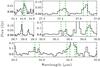 |
Fig. 10 OH emission lines (vertical dashed lines) in the Spitzer/IRS spectrum of IRAS 4B. The lines expected to be strongest are either detected (Table 2) or are blended with lines of other species. |
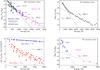 |
Fig. 11 Excitation diagrams, in units of total number of detected molecules |
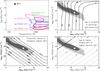 |
Fig. 12 Upper left: contours of χ2 versus temperature and H2 density for several different H2O column densities (the different colors), with the minimum reduced χ2 ~ 4. The contours show where |

4.2. Comparing H2O spectra for warm, subthermal excitation and cool, thermalized gas
The high temperature, low density solution presented here (hereafter H12, with properties obtained from the χ2 fit listed above) produces sub-thermal excitation of H2O, in contrast to the high-density (thermalized, with log n ~ 11, log N(H2O) = 17.0, and T = 170 K), low-temperature solution from Watson et al. (2007, hereafter W07). The W07 slab has many optically-thick lines, which leads to a spectrum where the mid-IR H2O lines observed with Spitzer are brighter than those in the PACS wavelength range (Fig. 14). In contrast, many of the far-IR lines in the H12 parameters are optically-thin, so that most H2O emission escapes in the PACS wavelength range. As a consequence, in principle the far-IR H2O emission could trace a high temperature, low density region (H12) while the mid-IR H2O emission traces a high density, low temperature component (W07).
The W07 model produces optically-thick emission in the o-H2O 818 − 707 and p-H2O 808 − 717 lines at 63.4 μm, with a flux in the p-H2O 808 − 717 line similar to the observed flux. However, the two lines are observed in an optically-thin flux ratio both on-source and at the blueshifted outflow lobe. Therefore, the W07 model cannot explain the PACS H2O emission located at the outflow position. If the extinction in W07 is reduced to AV ~ 0 mag, then the two 63.4 μm lines both become two times weaker relative to the mid-IR H2O lines.
A comparison between the Spitzer/IRS spectrum and the synthetic H2O spectrum (see Fig. 15 and a further discussion of line ratios in Appendix C) shows that both the W07 and H12 models could explain the mid-IR H2O emission alone. Both models are able to accurately reproduce the emission in most detected lines, with a few notable exceptions. The p-H2O 835 − 726 28.9 μm line flux is well reproduced in W07 but not H12. However, the wavelength of this line is more consistent with an OH line than with the H2O line. The OH rotational diagram (Fig. 11) shows that the line flux is also consistent with fluxes in other OH lines with similar excitations. The inability of H12 to reproduce this line flux with an H2O model is therefore not significant. An OH line at 24.6 μm was also misidentified as o-H2O 863 − 836 despite neither W07 nor H12 being able to produce flux in the H2O line. Because the synthetic fluxes of these lines are faint, the misidentification of this emission as H2O can help to drive a best fit physical parameters to an optically thick solution.
In models with high N(H2O) and n(H2), including W07, the line blend of o-H2O 652−523 and 550 − 423 at 22.4 μm and the p-H2O 642−515 23.2 μm line are predicted to be strong but are not detected. Both W07 and H12 overpredict the flux in the H2O 21.15 μm line. The H12 model does not significantly overpredict any other line in the IRS spectrum, even if the best fit H12 fluxes are scaled to the level of the strongest IRS lines rather than to the far-IR PACS lines.
This analysis demonstrates that a high temperature, low density model (H12) of the H2O emitting region can reasonably reproduce both the PACS and IRS spectra. On the other hand, a low temperature, high density model (W07) cannot reproduce the PACS spectrum, is inconsistent with the spatial distribution of the H2O 63.4 μm line emission, and overpredicts the emission in several lines in the IRS spectrum.
4.3. CO excitation
In the CO excitation diagram, a cool (280 ± 30 K) component dominates mid-J lines and a warm (880 ± 100 K) component dominates high-J lines. The uncertainty in temperature includes the choice of energy levels to fit for the high and cool components. The two excitation components could relate to regions with different kinetic temperatures or with different densities. RADEX models of CO were run using molecular data obtained from LAMDA (Schöier et al. 2005; Yang et al. 2010) with an extrapolation of collision rates up to J = 80 by (Neufeld 2012).
The detection of high-J CO lines with an excitation temperature of ~880 K requires log n(H2) > 6 for reasonable kinetic temperatures (<4000 K). For T = 1500 K, log n(H2) = 6.5, and an emitting area with radius 100 AU, the physical parameters adopted to explain the water emission, produces an excitation temperature of 950 K for lines with J = 30−45. This temperature is sensitive to the density, with log n(H2) = 6.0 leading to an excitation temperature of 640 K. The total number of CO molecules,  , for log n(H2) = 6.5 is
  .
.
In principle the two temperature components could relate to a single region with high temperature (~4000 K) and log n(H2) < 4 (Neufeld 2012). In this case, the CO emission would be physically unrelated to the highly excited H2O emission, and the CO abundance in the highly excited H2O emission region would be much smaller than that measured here.
4.4. OH excitation
The OH excitation diagram shows cool (60 ± 15 K) and warm (425 ± 100 K) components. RADEX models of the low excitation levels of OH (Eup < 1000 K) were run, using collisional rate coefficients from (Offer et al. 1994) and energy levels and Einstein A values from (Pickett et al. 1998). Molecular data for higher excitation levels were obtained from HITRAN (Rothman et al. 2009). A 1500 K gas with log n(H2) = 6.5 and emitting area of radius 100 AU roughly reproduces the emission in the cool component OH emission, with log N(OH) = 17.3. Whether these parameters could also reproduce the highly excited OH emission is not clear.
The RADEX model fluxes are also somewhat discrepant with the observed fluxes, The 24.6 μm line flux is much lower than predicted. In addition, all detected OH doublets have similar line fluxes but the RADEX model predicts different fluxes in several transitions. A lower opacity, caused either by broader lines or a lower column density and larger emitting area, would alleviate some of these discrepancies.
The OH molecule has energy levels with high critical densities and with strong far-IR transitions to low energy levels that are favorable to IR photoexcitation. Radiative pumping may therefore severely alter the level populations (e.g. Wampfler et al. 2010). The IR pumping would increase the populations in excited levels, which may cause us to overestimate the total number of OH molecules for the given temperature and density. As with H2O, a rigorous assessment of the IR pumping requires a full physical model of the envelope and is beyond the scope of this work.
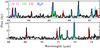 |
Fig. 13 Segments of the PACS spectrum (solid black line). The H2O line fluxes (shaded in blue) are obtained from RADEX, CO line fluxes (red) from the thermal distribution in Fig. 11, and OH (green) and [O I] line fluxes (purple) from Gaussian fits. |
4.5. O excitation
From the 63.18 μm line flux and assuming T = 1500 K, the total number of neutral O atoms is  . This number is robust to changes in temperature and density within the parameter space discussed here, based on RADEX models of [O I] lines. If the [O I] emission is spread out over a circle of 100 AU in radius, the column density log N(O) = 16.5 is much less than the column density required for the line to become optically thick (log N(O) ~ 19 for a Gaussian profile with a FWHM of 25 km s-1). These physical properties are adopted from the H2O emission for simplicity but are likely incorrect because the location of [O I] emission is spatially different than the H2O emission (left panel of Fig. 6).
5. Discussion
5.1. The origin of highly-excited H2O emission
Prior to this work, H2O emission has been attributed to three different regions in or near the IRAS 4B environment:
-
(1)
A compact disk: spectrally narrow (FWHM ~ 1 km s-1) H
O emission is produced in a (pseudo)-disk with a radius ~25 AU around IRAS 4B (Jørgensen & van Dishoeck 2010). From the inferred HO column density, the compact disk is optically-thick in most H O rotational transitions. The disk covers only a small area on the sky and therefore contributes very little emission to the broad lines detected with HIFI and to the mid- and far-IR H2O emission. From the assumed T = 170 K and resulting column density log N(p-H2O) ~ 18.4 and b = 1 km s-1, the p-HO 331 − 202 138.5 μm line, from the same upper level as the observed HO line, would have a flux of 3 × 10-22 W m-2, 50 times smaller than the measured line flux. Our PACS observations are unable to probe this disk component.
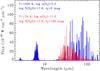
Fig. 14 The synthetic spectra for the H12 (blue) and W07 (red) models at a spectral resolution R = 1500. Because the W07 models are optically-thick in many highly-excited levels, the strongest H2O lines peak in the mid-IR rather than the far-IR. The H12 model predicts some rovibrational emission at 6 μm because of the high temperature, with a strength that could further constrain the temperature and density of the highly excited H2O.
-
(2)
Outflow emission, (a) in low-excitation lines with a large beam: spectrally-broad emission in low-excitation H2O lines was observed in spatially-unresolved observations over a ~20−40′′ beam and was attributed to outflows based on the line widths (Kristensen et al. 2010). The outflow is compact on the sky, so that both the red- and blue-shifted outflow lobes are located within this aperture.And (b), in masers: spectrally narrow (~1 km s-1) and spatially compact H2O maser emission is seen from dense gas in an outflow (e.g. Desmurs et al. 2009). The relationship between the maser emission and the molecular outflow is unclear.
-
(3)
Disk-envelope shock: H2O emission in highly-excited mid-IR lines, which are spectrally and spatially-unresolved at low spectral and spatial resolution, was attributed to the disk-envelope accretion shock (Watson et al. 2007). The primary argument for the accretion shock is that high H2 densities (>1010 cm-3) are needed to populate the highly excited levels, which have high critical densities. Such high densities are expected in an envelope-disk accretion shock but are physically unrealistic for an outflow-envelope accretion shock because envelope densities are much lower than disk densities.
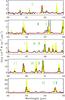 |
Fig. 15 A comparison of H12 (red dashed line, scaled to the flux in the 63.4 μm lines) and W07 (yellow filled regions, scaled to the flux of the 35.5 μm line) model spectra to the Spitzer IRS spectrum. Green vertical lines mark the wavelengths of OH lines that are detected (solid lines) or are too weak or blended to be detected (dotted lines). Both models reproduce most Spitzer/IRS lines reasonably well, with a few exceptions described in detail in the text. |
Our primary goals in this work are to use the spatial distribution and excitation of warm H2O emission to test (3), the envelope-disk accretion shock interpretation proposed by Watson et al. (2007), and to subsequently use the far-IR emission to probe the heating and cooling where the emission is produced. In the following subsections, we discuss the outflow origin of the highly-excited H2O emission and subsequently discuss the implications for the envelope-disk accretion shock and outflows.
5.2. Outflow origin of highly excited H2O emission
The H2O emission detected with PACS is spatially offset from the peak of the far-IR continuum emission to the south, the direction of the blueshifted outflow. Of the mapped lines, the H2O 818−707 and 808−717 lines at 63.4 μm are closest in excitation to the mid-IR Spitzer lines. The location of the emission in both 63.4 μm H2O lines is consistent with the location of near-IR emission from IRAS 4B imaged with Spitzer/IRAC. The full PACS spectrum from 50−200 μm demonstrates that all other molecular lines are also offset from the location of the sub-mm continuum peak (Fig. 5). These lines are produced in the southern, blueshifted outflow lobe of IRAS 4B, as shown in the plots and cartoon of Figs. 6, 7.Contemporaneous to our work, Tappe et al. (2012) found that the spatial distribution of H2O emission in Spitzer/IRS spectra is consistent with an outflow origin. The images of CO 24–23 and 49–48 also demonstrate that highly excited CO emission is produced in the blueshifted outflow lobe. The CO 49–48 emission is located closer to the central source than the highly excited H2O emission.
The combined Herschel/PACS and Spitzer/IRS excitation diagram does not show any indication of multiple components in the highly-excited H2O lines. RADEX models indicate that the highly excited PACS lines are consistent with emission from a single slab of gas with T ~ 1500 K, log N(H2O) ~ 17.6, log n ~ 6.5, and an emitting area equivalent to a circle with radius ~100 AU. The same parameters reproduce the mid-IR H2O emission lines detected in the Spitzer/IRS spectrum of IRAS 4B. These same physical conditions may also produce CO fundamental emission, which could explain the bright IRAC 4.5 μm emission from the IRAS 4B outflow (Tappe et al. 2012).
The on-source component of the far-IR H2O is not as well described as the outflow component because this component is faint in the short wavelength PACS lines, which are able to constrain the properties of the emission at the offset outflow position. The on-source emission suffers from higher extinction, so the brightest lines are at longer wavelengths, have low excitation energies, and are optically thick. Our RADEX modeling is restricted to the higher excitation component of the H2O emission. However, the similarity of the ratio of the two 63.4 μm lines at the sub-mm continuum location and at the outflow location suggests similar excitations. The non-detection of HO lines (see Appendix C) place a strict limit on the optical depth of the H2O lines. The H2O 108.1 μm line, of which 70% is located on-source, likely traces the same material as the HIFI spectra of low-excitation H2O lines (Kristensen et al. 2010). The width of the HIFI emission (FWHM ~ 24 km s-1, with wings that extend out to ~80 km s-1) is consistent with an outflow origin and inconsistent with a slow (~2 km s-1) envelope disk accretion shock that would be expected for infalling gas.
In sub-mm line emission, both the red- and blueshifted outflows are detected and spatially separated (Jørgensen et al. 2007; Yildiz et al. submitted), which indicates that the outflow is not aligned exactly along our line of sight to the central object. In previous near- and mid-IR imaging, only the blueshifted outflow is detected and the redshifted outflow is invisible. The extinction to the redshifted outflow is so high that even the far-IR emission is obscured by the envelope. The outflow therefore cannot be aligned in the plane of the sky and likely is aligned to within 45° of our line of sight to the central star. This large extinction is consistent with the outflow angle of ~15° relative to our line of sight, as inferred from assuming that the IRAS 4B outflow has the same age as the IRAS 4A outflow (Yıldız et al. 2012).
The relationship between the outflow and the maser emission is uncertain. The maser emission has a position angle of 151° from IRAS 4B (Park & Choi 2007; Marvel et al. 2008; Desmurs et al. 2009), in contrast to the ~174° position angle of the molecular outflow (Jørgensen et al. 2007). Unlike the molecular outflow, the maser emission is located in the plane of the sky (~77° relative to our line of sight), based on the radial velocity and projected velocity on the sky. In this case, the outflow would have a dynamical age of only 100 yr. However, the high extinction to the redshifted outflow and low extinction to the blueshifted outflow together suggest that the outflow is aligned closer to our line of sight than in the plane of the sky. Jet precession, perhaps a result of binarity of the central object, has been suggested as a possible explanation for the difference between the maser emission and molecular outflow (Desmurs et al. 2009).
H2O maser emission is produced in gas with densities of 107−109 cm-3 (Kaufman & Neufeld 1996). The density of the far-IR H2O emission could be as high as ~107 cm-3. However, the maser emission is produced in very small spots within the outflow, while the H2O emission detected here is likely spread over a projected area equivalent to a circle with a radius ~100 AU. In principle, the maser emission could simply be the smallest, densest regions within the same outflow that produces the far-IR H2O emission, although the maser and far-IR H2 emission may be unrelated.
In summary, we conclude that most of the H2O emission from IRAS 4B is produced in the blueshifted outflow. The highly excited H2O emission is located at the blueshifted outflow position. The redshifted outflow is likely not detected in these lines because any emission is obscured by the envelope. The optically thick lower-excitation H2O lines have an additional on-source component and are likely similar to the spectrally broad outflow seen by Kristensen et al. (2010). Similarly, the cool components of OH and CO emission are also likely produced in the outflow rather than a quiescent envelope.
Summary of components for H2O emission from IRAS 4B.
5.3. Implications for envelope-disk accretion
The primary motivation for invoking the envelope-disk accretion shock to interpret the mid-IR H2O lines was the high critical densities for the mid-IR H2O lines. We have demonstrated that these lines may also be produced in gas with sub-thermal excitation. An additional component besides the outflow does not need to be invoked at present to explain the presence of the mid-IR H2O emission.
The envelope-disk accretion shock may still have some undetected contribution to the on-source H2O emission seen with PACS, in which case the mid-IR H2O emission could in principle be the combination of the blueshifted outflow lobe and the envelope-disk accretion shock. The Watson et al. (2007) interpretation of the H2O emission requires high line optical depths, including in the 63.4 μm H2O lines. However, the 63.4 μm H2O ortho/para lines are observed at the optically-thin flux ratio, with an upper limit that no more than 30% of the observed emission may be produced in optically thick gas. Since the envelope-disk accretion shock would only contribute to the on-source emission, the maximum contribution to the total flux in the 63.4 μm lines is ~10%. In this case, we find that the luminosity of the disk-envelope accretion shock would be 1.5 × 10⁻³ L⊙, 5% of that calculated by Watson et al. (2007)6. The accretion rate onto the disk would correspond with ~3 × 10⁻⁶ M⊙ yr-1, which is likely too low to represent the main phase of disk growth.
An alternate and likely explanation is that any disk-envelope accretion shock is buried inside the envelope, with an extinction that prevents the detection of any mid-IR emission produced by such a shock. The on-source H2O and CO emission is likely produced in an outflow that is seen behind AV ~ 700 mag of extinction. In this case, whether the envelope-disk accretion shock exists is uncertain and the accretion rate is completely unconstrained. The prospects for studying envelope-disk accretion likely require a high-density (>1011 cm-3) tracer (Blake et al. 1994) observed at high spatial and spectral resolution in the sub-mm, where emission is not affected by extinction.
5.4. Gas line cooling budget and abundances for IRAS 4B
The bulk of the far-IR line emission is produced in the outflow. The emission is smoothly distributed within the outflow and is consistent with emission from two different positions, one located on-source and one located off-source.
Table 3 lists the total cooling budget attributed to the molecular and atomic emission in the far-IR, as extracted from the on-source position and the blueshifted outflow lobe. Most of the cooling is in molecular lines rather than atomic lines, which is consistent with previous estimates of far-IR cooling from a larger sample of Class 0 objects that were observed with ISO (Nisini et al. 2002).
In contrast to the luminous molecular lines, the [O I] emission from IRAS 4B is surprisingly faint. The [O I] 63 μm line is typically the brightest far-IR emission line from low-mass protostars, with an average luminosity of 10-3 Lbol for Class 0 stars and 10-2 Lbol for Class I stars (Giannini et al. 2001; Nisini et al. 2002). For IRAS 4B, the [O I] flux is 10-3.5 Lbol. The weak [O I] emission may be a signature of the youngest protostars with outflows that have not yet escaped the dense envelope, as may be the case for IRAS 4B. Although some [O I] emission could be located behind the envelope for IRAS 4B and other Class 0 objects, the non-detection of the [O I] 145.5 μm line suggests that neglecting extinction does not lead to a serious underestimate in [O I] line lumonosity. The PACS spectrum also does not show any evidence for high-velocity [O I] emission from the jet, unlike the more evolved embedded object HH 46 (van Kempen et al. 2010a).
The abundance ratio7 OH/H2O ~ 0.2 is consistent with the abundance ratio OH/H2O > 0.03 for the outflow from the high-mass YSO W3 IRS 5 (Wampfler et al. 2011), the only other YSO with such a measurement. The H2O/CO abundance is ~1, on the high end of the value of 0.1 − 1 found from emission in lower-excitation lines of CO and H2O (Kristensen et al. 2010). The ratio of H2O/H2 is ~ 10-4, based on the total number of H2 molecules ( ) calculated from the extinction corrected fluxes of pure-rotational H2 lines from (Tappe et al. 2012). The H2 and H2O emission trace the same projected region on the sky (right panel of Fig. 6, with the Spitzer/IRAC imaging dominated by H2 emission).
The abundance ratio of O/H2O is ~ 0.1 for the detected emission in the blueshifted outflow. The [O I] emission is predominately located alongside the outflow axis and is offset from the location of the H2O emission. Within the shock that produces the highly excited H2O emission, the O/H2O abundance ratio must be much lower than 0.1. The non-detection of [C II] emission suggests that the ionization fraction in the shock is low. At least 90% of the gas-phase O is in H2O, CO, and OH, which is consistent with the high H2O/H2 ratio measured above.
Relative to other sources, the listed H2O column density is ~102 − 104 times larger than that found from L1157 (Nisini et al. 2010; Vasta et al. 2012). Some of this discrepancy might be attributed to methodology. The H2O column density calculated here is measured directly from the opacities in many different lines, which are spectrally unresolved. In contrast, the H2O column density is calculated from optically thick lines, many of which are spectrally resolved but measured with a range of beam sizes. However, the H2O abundance from IRAS 4B may be much larger than that of most other young stellar objects, possibly because of some physical difference in the outflow properties.
5.5. Shock properties for the highly excited molecular outflow
The H2O line cooling is qualitatively consistent with excitation of molecular gas predicted from C-shocks by Kaufman & Neufeld (1996). The OH emission also likely traces shocks because OH has a high critical density and is an intermediate in the high temperature gas phase chemistry that produces H2O. The two-temperature shape of the CO excitation diagram is expected from models of shock and UV-excitation of outflow cavity walls (Visser et al. 2011) and is qualitatively consistent with similar observations of the Class I sources HH 46 and DK Cha (van Kempen et al. 2010ab). The ratio of H2O to CO luminosity is higher for IRAS 4B than for the Class I source HH 46 and for the borderline Class I/II source DK Cha. These differences may indicate that shock heating of the envelope plays a more important role than UV heating during the Class 0 stage. Indeed, Visser et al. (2011) suggested an evolutionary trend that for more massive and denser (younger) envelopes the shock heating should dominate. The different evolutionary stages may not change the shape of the CO ladder, as the relative contributions of the mid-J (15–25) and high-J (25–50) CO lines are similar for DK Cha and IRAS 4B. The highly excited H2O emission may also be especially strong from IRAS 4B because the outflow covers only a very compact area when projected on the sky.
Highly excited H2O and OH lines were previously detected in mid-IR Spitzer/IRS spectra of the HH 211 bow shock, which is strong enough (~200 km s-1) to dissociate molecules at the location of direct impact. Such a high velocity shock also produces strong UV radiation (see models by Neufeld & Dalgarno 1989 and observations by, e.g., Raymond et al. 1997 and Walter et al. 2003) that photodissociates molecules both upstream and downstream of the shock. In Fig. 2 of Tappe et al. (2008), many mid-IR OH emission lines are stronger than the H2O lines from HH 211. In contrast, the mid-IR H2O lines are much stronger than the mid-IR OH lines from IRAS 4B. In addition, the OH emission from HH 211 is detected from levels with much higher excitation energies than detected here, in a pattern that is consistent with prompt emission following production of OH in excited levels through photodissociation of H2O by far-UV radiation (presumably Lyman α, Tappe et al., 2008). The atomic fine-structure lines are also brighter from the HH 211 outflow than from IRAS 4B (Giannini et al. 2001; Tappe et al. 2008). Thus, UV radiation likely plays a large role in both the chemistry and excitation of OH at the HH 211 shock position, which is well separated from the YSO itself and is outside the densest part of the envelope.
In the case of IRAS 4B, the combination of bright H2O emission and faint [O I] emission suggests that the H2O dissociation rate is low. Moreover, the OH emission from IRAS 4B is not seen from the very highly excited levels detected from HH 211. Thus, OH likely forms through the traditional route of high temperature (>230 K) chemistry of reactions between O and H2 to form OH. The OH can then collide with H2 to form H2O. These reactions control the oxygen chemistry in dense C-type shocks (Draine et al. 1983; Kaufman & Neufeld 1996). The balance between O, OH and H2O in well-shielded regions depends primarily on the H/H2 ratio of the gas. In dense photo-dissociation regions, these same high temperature reactions are effective in forming H2O, but the strong UV field can drive H2O back into O and H2O (Sternberg et al. 1995). Indeed, for the Orion Bar, the very strong UV field leads to a higher OH/H2O abundance ratio (OH/H2O > 1) than detected here (OH/H2O ~ 0.1), in addition to emission in other diagnostics of strong UV radiation (strong [C II] and CH+ emission) that are detected from the Orion Bar (Goicoechea et al. 2011) but are not detected from IRAS 4B. Thus, the C-shock that produces the OH and H2O emission from IRAS 4B is likely not irradiated by UV emission. The shocked gas may be shielded from any UV emission produced by the central source and internal shocks within the jet.
This shielding lends support to a C-type shock explanation rather than molecular formation downstream of a dissociative J-type shock because such a shock would produce UV emission (see discussion above). A non-dissociative shock is also consistent with the presence of H2 emission from IRAS 4B (Arnold et al. 2011; Tappe et al. 2012). This scenario is different than that postulated for HH 46 by (van Kempen et al. 2010a), where the on-source O and OH emission was thought to be produced by a fast dissociative J-type shock based on the different spatial extents of OH and H2O. This scenario also differs from the interpretation of Wampfler et al. (2011) that the OH and H2O emission from the high-mass YSO W3 IRS 5 arises either in a J-type shock or in a a UV-irradiated C-shock. While the J-type shock or UV-irradiated C-type shock is an unlikely explanation for the H2O emission, the OH emission could be produced in a different location than the H2O emission, as is the case for [O I].
6. Conclusions
We have analyzed Herschel/PACS spectral images of far- IR H2O emission from the prototypical Class 0 YSO IRAS 4B. Table 5 summarizes the different components of H2O emission from IRAS 4B. We obtained the following results:
-
1)
A rich forest of highly-excited H2O, OH, and CO emission lines is detected in the blueshifted outflow from IRAS 4B. The spectrum is more line-rich than any other low-mass YSO that has been previously published.
-
2)
Nyquist-sampled spectral maps place the highly-excited 63.4 μm lines at a average distance of
(projected distance of 1130 AU) south of IRAS 4B. The lower-excitation H2O 108.1 μm line has a centroid closer to the peak of the sub-mm continuum emission and has a larger spatial extent than the 63.4 μm emission along the outflow axis. The far-IR H2O emission can be interpreted as one component located at the blueshifted outflow position and a second component at the peak position in the mass distribution (sub-mm continuum peak). The redshifted outflow lobe is not detected in highly-excited H2O emission, likely because of a high extinction (>1500 mag) through to the back side of the envelope. -
3)
The highest excitation lines detected with PACS are optically-thin, indicating an ortho-to-para ratio of ~3. RADEX models of the highly excited H2O lines indicate that the emission is produced in gas described by T ~ 1500 K, log n(H2) ~ 6.5 cm-3, and log N(H2O) ~ 17.6 cm-2 over an emitting area equivalent to a circle with radius ~100 AU. These same physicals parameters can reproduce the mid-IR H2O emission seen with Spitzer/IRS and the CO and OH emission seen with PACS. The total mass of warm H2O in the IRAS 4B outflow is about 140 times the amount of water on Earth.
-
4)
From results (2) and (3), we conclude that the bulk of the far-IR H2O emission is produced in outflows. Any contribution of the envelope-disk accretion shock to highly-excited H2O lines is minimal. Moreover, at present the mid-IR H2O emission does not offer any support for the presence of an envelope-disk accretion shock, as had been previously suggested by Watson et al. (2007). Any mid-IR H2O emission produced by the envelope-disk accretion shock is likely deeply embedded in the envelope.
-
5)
In the blueshifted outflow lobe over 90% of the gas phase O is in the H2O, CO, and OH molecules rather than in neutral O. The H2O is twice as abundance as CO and 10 times more abundant than OH. The cooling budget for gas in the envelope around IRAS 4B is dominated by H2O emission.
-
6)
The H2O emission traces high densities in non-dissociative C-shocks. In contrast, much of the heating of lower mass envelopes occurs by energetic radiation. The highly excited H2O in the shock-heated gas is likely shielded from UV radiation produced by both the central star and the bow shock. The OH likely forms through reactions between O and H2 and provides a pathway to form H2O.
Online material
Appendix A: Calibration of first and second order light longward of 190 μm
PACS spectra are poorly calibrated in regions where light from different orders are recorded at the same physical location on the detector, especially between 97–103 μm and longward of 190 μm. Most photons between 97–105 μm get dispersed into the second order and contaminate the flux at >190 μm because of a mismatch between the grating and the filter transmission. Similarly, the light at 97–103 μm can be contaminated by third-order emission at ~69 μm. As a consequence, the first order light at 97–103 μm has low S/N and that light and the light at >190 μm has not previously been flux calibrated. In this appendix, we use PACS spectra of Serpens SMM 1 (Goicoechea et al., in prep.) and HD 100546 (Sturm et al. 2010), both reduced in the same method as IRAS 4B, to calibrate the first and second order emission from PACS at λ > 190 μm. The continuum emission from HD 100546 is produced by a disk and peaks (in Jy) at ~60 μm. The continuum emission from Serpens SMM 1 is produced in an envelope and peaks at ~150 μm.
First and second order light can be separated because the diffraction-limited point spread function is twice as large at 200 μm as at 100 μm. Figure A.1 shows the fraction of flux in the central spaxel divided by the flux in the central 3 × 3 spaxels. This fraction decreases smoothly at >100 μm. The fraction starts to rise at ~190 μm because of a contribution from second order emission. At each wavelength, this fraction directly leads to a ratio of first order photons to second order photons recorded by PACS. The second order light is then calibrated by measuring the first order light between 90–110 μm for HD 100546. Most of the light recorded at >190 μm from HD 100546 is second order light.
This calibration is then applied in reverse to the spectrum of Serpens SMM 1 to subtract the second order emission, leaving only first order emission at >190 μm. A SPIRE spectrum of Serpens SMM 1 (Goicoechea et al., in prep.) is then used to flux calibrate the PACS spectrum from 190–210 μm. Despite the red spectrum of Serpens SMM 1, ~50% of the photons recorded at 202 μm are second-order 101 μm photons.
To calibrate the PACS spectrum of IRAS 4B, the first and second order light are initially separated based on the point spread function for both wavelengths (Fig. A.1). The separate first and second order spectra are then flux calibrated using the relationships calculated above. Lines are identified as first or second order emission after searching for the correct line identification at λ and λ/2.
Figure A.2 shows the resulting spectrum of IRAS 4B at 95–105 μm. Analysis of a large sample of PACS spectra from the DIGIT program (P. I. N. Evans) suggest that our flux calibration has an uncertainty of ~20% between 98–103 μm, in addition to other sources of uncertainty in the standard PACS flux calibration. The line fluxes measured from second order light at >190 μm are consistent to 20% of the fluxes measured directly at 97–103 μm but with smaller error bars. The accuracy of the flux calibration at >190 μm has not been evaluated but is likely uncertain to ~40%.
The best place to observe lines between 98–103 μm with PACS is in the second order, despite overlap with first-order light because of sensitivity and higher spectral resolution. The PACS sensitivity to first order photons at >200 μm is low. This new calibration allows us to improve the accuracy of flux measurements for lines between 98–103 μm and at >190 μm.
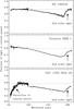 |
Fig. A.1 The ratio of flux in the central spaxel to the flux in the central 3 × 3 spaxels for HD 100546, Serpens SMM 1, and NGC 1333 IRAS 4B. The ratio falls linearly above >100 μm until 190 μm. Second order light contaminates the spectrum at >190. Because the first and second order light have different point-spread functions, the plotted ratio determines the fraction of first and second order photons versus wavelength. For NGC 1333 IRAS 4B, the continuum flux in the central spaxel falls at <70 μm, likely because of extinction. |
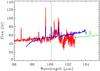 |
Fig. A.2 The first and second order spectrum of IRAS 4B at ~100 μm. The second order light at 100 μm (blue), calibrated from the ~200 μm spectrum, matches the standard first and second order spectra (red and green). The lines in the blue spectrum are artificially weak, by a factor equivalent to the ratio of first to second order light, because the lines and continuum are treated separately. The dotted vertical line shows the location of the CO 13–12 line at 200.27 μm. |
Appendix B: Unidentified lines
All strong lines in the IRAS 4B spectrum are identified. Table B.1 lists several possible lines that are detected at the ~3 σ significance level. The position of several of these tentative detections do not correspond to expected emission lines. Although no o-HO are clearly detected, the o-HO 212 − 110 109.346 μm line is expected to be among the strongest HO lines and is tentatively detected. The centroid of the detected emission is − 170 km s-1 from the expected centroid, based on the measured wavelengths of other nearby lines. Emission is detected consistent with the location of the p-H2O 551 − 624 71.787 μm line, but the line flux is expected to be very weak.
These lines are all very weak and may be statistical fluctuations in the spectrum rather than significant detections of unidentified lines.
Appendix C: Exploring the parameter space in model fits to H2O line fluxes
In Sect. 4, we characterized the physical properties of the H2O emission region by comparing the observed line fluxes to synthetic fluxes calculated in RADEX models of a plane-parallel slab. In this appendix, we describe how the measured line fluxes constrain the parameters of the highly excited gas.
The backbone o-H2O lines 909−818, 818−707, 707 − 616, 616−505, 505−414 and their p-H2O counterparts are amongst the best diagnostics for the excitation and optical depth of the H2O emitting region. The relative flux calibration between these ortho/para pairs should be accurate to better than 5% because the lines are located very near each other. The flux ratio ranges from 2.8–3.5 in the three of the backbone line ratios with highest excitation, indicating that the ortho-to-para ratio of ~3 is thermalized and that these lines are optically-thin. The 616−505, 505 − 414, and 414 − 303 and their p-H2O counterparts have flux ratios of ~2.3−2.5, suggesting that either the modeled emission is moderately optically thick in these lines, or that a second, optically-thick component contributes some emission to the flux in lower-excitation, longer wavelength lines. The top panels of Fig. C.1 show the acceptable space of n(H2) and T for two different values of N(H2O) based on two of these line ratios.
The χ2 statistic automates this type of analysis over all of the applicable lines to find the best-fit parameters for a single isothermal slab. Limiting the χ2 calculation to lines with E′ > 600 K yields two acceptable parameter spaces, one at the H12 location (T ~ 1500 K, log n(H2) ~ 6.5, and log N(H2O) ~ 17.6) and one at low-temperature, high density, and low column density (hereafter X11, with T ~ 200 K, log n(H2) ~ 11, and log N(H2O) ~ 14.0). The X11 parameters differ from W07 because W07 includes a large H2O column density to produce optically thick lines. The X11 parameters are disqualified because several lines, such as o-H2O 330 − 221 66.44 μm, have a synthetic flux that is much stronger than the observed emission8. As a consequence, the χ2 statistic for all lines with E′ > 400 K yields acceptable line fluxes only around the H12 parameters, adopted in this paper, and disqualifies the X11 parameter space.
The o-H2O transitions 550−541 at 75.91 μm and 652 − 643 at 75.83 μm have a 2σ upper limit on the combined flux of 3 × 10-21 W cm-2. Although these upper limits are not included in the χ2 calculations, the non-detections confirm that the parameter space with high H2 density and high H2O column density cannot explain the bulk of the far-IR H2O emission (lower left panel of Fig. C.1). Similarly, the line ratio o-H2O 845 − 734 35.67 μm to o-H2O 707 − 616 71.95 yields physical parameters consistent with the best-fit solution (lower right panel of Fig. C.1).
The non-detection of emission in HO lines (with the possible exception of o-HO 212 − 110 109.35 μm) also places a limit on the opacity of HO lines. The bottom right panel of Fig. C.1 shows where the flux ratio of o-HO 321 − 212 75.87 μm to o-H2O 616 − 505 82.03 μm becomes >50, large enough that the HO line would be detected. This upper limit rules out the parameter space of high density and high column density.
In the H12 model, the strength of the 6 μm continuum emission (Maret et al. 2009) is similar to the strength of the 6 μm rovibrational H2O lines. The non-detection with R = 60 spectra is marginally consistent with the predicted emission and rules out temperatures higher than ~ 2000 K. An AV = 20 mag. would reduce the predicted 6 μm emission by 35%. Decreasing the temperature from 1500 K to 1000 K would reduce the predicted 6 μm emission by a factor of 4.8. Measurements of emission in H2O vibrational lines would place significant additional constraints on the properties of the H2O emission.
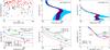 |
Fig. C.1 H2O fluxes and acceptable parameter space of temperature and H2 density. The upper left panel shows that in the H12 model, all far-IR H2O lines expected to be strong are detected (red dots), while those expected to be weak are undetected (black dots). Several lines at ~100 μm were likely undetected because the S/N is degraded in that wavelength region. The upper middle panel shows the acceptable contours for flux ratios of o-H2O 818−707/707−616 (blue), o-H2O 707−616/616−505 (red), and both (purple), for two different column densities. The acceptable parameter space shows the 1σ error bars with a 20% relative flux calibration uncertainty. The lower left panel shows that the non-detection of the o-H2O 550−541 and 652−643 lines relative to o-H2O 616 − 505 line places a limit on the optical depth of the slab. The lower middle panel shows where the flux ratio of o-H2O 845−734 35.669 μm to o-H2O 707−616 71.947 μm is equal to the observed value of 0.07. The lower right panel shows the parameter space (high density and high column density) ruled out by the non-detection of the o-H |
Appendix D: Effect of extinction estimates on rotational diagrams
Extinction can affect the derivation of excitation temperatures and line luminosities, especially at shorter wavelengths where lines typically have upper levels with higher energies. In this analysis, we assume that for all H2O lines, 70% of the luminosity is produced on source behind AV = 700 mag. and 30% is produced off-source at the blueshifted outflow lobe, with AV = 0 mag. (see also Sect. 4.3). This description is consistent with the different observed spatial distributions of the H2O 108.1 and 63.4 μm lines. The excitation conditions and emission line ratios may instead vary smoothly with distance in the outflow.
Applying an extinction correction under these assumptions increases the excitation temperature of the warm (cool) CO component from 850 to 950 K (250 to 280 K). If all the CO emission were located behind the AV = 700 mag., then the temperature difference would become much larger, but the short wavelength CO lines would be very faint. The H2O temperature does not change significantly because the fits are based mostly on lines at short wavelengths, so the emission from the heavily embedded region is mostly extinguished. An AV = 100 mag to the blue outflow lobe would increase the relative luminosity of lines at 25 μm compared with those at 100 μm by a factor of four,
thereby increasing the warm H2O excitation temperature from 220 K to 240 K. An AV > 200 mag to the outflow is ruled out by the significant increase in scatter in the excitation diagram.
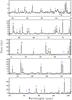 |
Fig. D.1 The continuum-subtracted PACS spectrum of NGC 1333 IRAS 4B from 55–100 μm. The marks identify lines of H2O (blue), CO (red), OH (green), and [O I] (purple). |
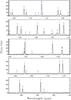 |
Fig. D.2 The continuum-subtracted PACS spectrum of NGC 1333 IRAS 4B from 103–195 μm. The marks identify lines of H2O (blue), CO (red), and OH (green). |
Detected lines in Herschel/PACS spectrum of IRAS 4B.
The optical guider observations onboard Herschel are typically accurate to ~1′′. However, observations of nearby high-extinction regions, including NGC 1333 IRAS 4B, have few optical guide stars, which may introduce pointing offsets when the few guide stars are distributed asymmetrically in the field-of-view.
Throughout the paper all logarithms are base 10, all units for column density are in cm-2, and all units for density are cm-3. The units in excitation diagrams are in number of detected molecules rather than column density.
The terminology “warm” and “cool” components, as defined here, corresponds to “hot” and “warm” gas, respectively, in other works, including Visser et al. (2011), which considers colder gas, usually observed in the sub-mm, than the gas studied here.
The HIFI H2O lines are much more optically-thick and likely have larger emitting areas than most H2O lines in the PACS spectrum, which may lead to differences in line profile.
The rate is also adjusted from Watson et al. (2007) for updated distance of 235 pc.
As calculated from the highly excited H2O emission and the low temperature component of OH emission, both modeled with RADEX with the same temperature and density. It is unclear whether the warmer component of OH emission can be reproduced by these same parameters. The OH abundance may be severely affected by infrared pumping (Wampfler et al. 2010).
The opposite case, where the synthetic emission is weaker than observed in a low-excitation line, would not disqualify a model because low-excitation line emission may include an additional contribution from cooler gas.
Acknowledgments
G.J.H. thanks Achim Tappe for interesting and extensive discussions regarding the location of H2O in the Spitzer/IRS spectra and the outflow inclination, and for detailed comments on the manuscript. G.J.H. also thanks Tom Megeath for discussions regarding the comparison of Spitzer/IRS and Herschel/PACS spectra, and Mario Tafalla, Javier Goicoechea, the anonymous referee, and the editor, Malcolm Walmsley for careful reads of the manuscript and insightful comments, Per Bjerkelli, Jeong-Eun Lee, and Doug Johnstone for some useful comments, and Stefani Germanotta for help in preparing the manuscript. We also thank Javier Goicoechea for providing us with the SPIRE spectrum of Ser SMM1 and for use of some DIGIT data to help calibrate the PACS spectrum at long wavelengths. Astrochemistry in Leiden is supported by NOVA, by a Spinoza grant and grant 614.001.008 from NWO, and by EU FP7 grant 238258. The research of JKJ is supported by a Lundbeck Foundation Junior Group Leader Fellowship and by the Danish Research Council through the Centre for Star and Planet Formation.
References
- Adams, F. C., Lada, C. J., & Shu, F. H. 1987, ApJ, 312, 788 [NASA ADS] [CrossRef] [Google Scholar]
- André, P., Ward-Thompson, D., & Barsony, M. 1993, ApJ, 406, 122 [NASA ADS] [CrossRef] [Google Scholar]
- Arce, H., & Sargent, A. I. 2006, ApJ, 646, 1070 [NASA ADS] [CrossRef] [Google Scholar]
- Arnold, L. A., Watson, D. M., Kim, K. H., et al. 2011, ApJ, submitted [arXiv:1107.3261v2] [Google Scholar]
- Bergin, E. A., Kaufman, M. J., Melnick, G. J., Snell, R. L., & Howe, J. E. 2003, ApJ, 582, 830 [NASA ADS] [CrossRef] [Google Scholar]
- Blake, G. A., van Dishoeck, E. F., Jansen, D. J., Groesbeck, T. D., & Mundy, L. G. 1994, ApJ, 428, 680 [NASA ADS] [CrossRef] [Google Scholar]
- Bontemps, S., Andre, P., Terebey, S., & Cabrit, S. 1996, A&A, 311, 858 [NASA ADS] [Google Scholar]
- Chapman, N. L., Mundy, L. G., Lai, S.-P., & Evans, N. J. 2009, ApJ, 690, 496 [NASA ADS] [CrossRef] [Google Scholar]
- Choi, M., & Lee, J.-E. 2011, JKAS, 44, 201 [Google Scholar]
- Curiel, S., Raymond, J. C., Wolfire, M., et al. 1995, ApJ, 453, 322 [NASA ADS] [CrossRef] [Google Scholar]
- Desmurs, J.-F., Codella, C., Santiago-Garcia, J., Tafalla, M., & Bachiller, R. 2009, A&A, 498, 753 [Google Scholar]
- Di Francesco, J., Myers, P. C., Wilner, D. J., Ohashi, N., & Mardones, D. 2001, ApJ, 562, 770 [NASA ADS] [CrossRef] [Google Scholar]
- Draine, B. T., Roberge, W. G., & Dalgarno, A. 1983, ApJ, 264, 485 [NASA ADS] [CrossRef] [Google Scholar]
- Faure, A., & Josselin, E. 2008, A&A, 492, 257 [NASA ADS] [CrossRef] [EDP Sciences] [Google Scholar]
- Faure, A., Crimier, N., Ceccarelli, C., et al. 2007, A&A, 472, 1029 [NASA ADS] [CrossRef] [EDP Sciences] [Google Scholar]
- Furuya, R. S., Kitamura, Y., Wootten, A., Claussen, M. J., & Kawabe, R. 2003, ApJS, 144, 71 [NASA ADS] [CrossRef] [Google Scholar]
- Giannini, T., Nisini, B., & Lorenzetti, D. 2001, ApJ, 555, 40 [NASA ADS] [CrossRef] [Google Scholar]
- Goicoechea, J. R., Joblin, C., Contursi, A., et al. 2011, A&A, 530, L16 [NASA ADS] [CrossRef] [EDP Sciences] [Google Scholar]
- Gutermuth, R. A., Myers, P. C., Megeath, S. T., et al. 2008, ApJ, 674, 336 [NASA ADS] [CrossRef] [Google Scholar]
- Herczeg, G. J., Brown, J. M., van Dishoeck, E. F., & Pontoppidan, K. M. 2011, A&A, 533, A112 [NASA ADS] [CrossRef] [EDP Sciences] [Google Scholar]
- Hirota, T., Bushimata, T., Choi, Y. K., et al. 2008, PASJ, 60, 37 [NASA ADS] [CrossRef] [Google Scholar]
- Horne, K. 1986, PASP, 98, 609 [NASA ADS] [CrossRef] [EDP Sciences] [Google Scholar]
- Indebetouw, R., Mathis, J. S., Babler, B. L., et al. 2005, ApJ, 619, 931 [NASA ADS] [CrossRef] [Google Scholar]
- Jørgensen, J. K., & van Dishoeck, E. F. 2010, ApJ, 710, L72 [NASA ADS] [CrossRef] [Google Scholar]
- Jørgensen, J. K., Schöier, F. L., & van Dishoeck, E. F. 2002, A&A, 389, 908 [NASA ADS] [CrossRef] [EDP Sciences] [Google Scholar]
- Jørgensen, J. K., Harvey, P. M., Evans, N. J., et al. 2006, ApJ, 645, 1246 [NASA ADS] [CrossRef] [Google Scholar]
- Jørgensen, J. K., Bourke, T. L., Myers, P. C., et al. 2007, ApJ, 659, 479 [NASA ADS] [CrossRef] [Google Scholar]
- Jørgensen, J. K., van Dishoeck, E. F., Visser, R., et al. 2009, A&A, 507, 861 [NASA ADS] [CrossRef] [EDP Sciences] [Google Scholar]
- Kaufman, M. J., & Neufeld, D. A. 1996, ApJ, 456, 611 [NASA ADS] [CrossRef] [Google Scholar]
- Kirk, H., Johnstone, D., & Di Francesco, J. 2006, ApJ, 646, 1009 [NASA ADS] [CrossRef] [Google Scholar]
- Kristensen, L. E., Visser, R., van Dishoeck, E. F., et al. 2010, A&A, 521, L30 [NASA ADS] [CrossRef] [EDP Sciences] [Google Scholar]
- Liseau, R., Justtanont, K., & Tielens, A. G. G. M. 2006, A&A, 446, 561 [NASA ADS] [CrossRef] [EDP Sciences] [Google Scholar]
- Maret, S., Bergin, E. A., Neufeld, D. A., et al. 2009, ApJ, 698, 1244 [NASA ADS] [CrossRef] [Google Scholar]
- Marvel, K. B., Wilking, B. A., Claussen, M. J., & Wootten, A. 2008, ApJ, 685, 285 [NASA ADS] [CrossRef] [Google Scholar]
- Neufeld, D. A. 2010, ApJ, 708, 635 [NASA ADS] [CrossRef] [Google Scholar]
- Neufeld, D. A. 2012, ApJ, submitted [Google Scholar]
- Neufeld, D. A., & Dalgarno, A. 1989, ApJ, 344, 251 [NASA ADS] [CrossRef] [Google Scholar]
- Neufeld, D. A., & Hollenbach, D. J. 1994, ApJ, 428, 170 [NASA ADS] [CrossRef] [Google Scholar]
- Neufeld, D. A., & Yuan, Y. 2008, ApJ, 678, 974 [NASA ADS] [CrossRef] [Google Scholar]
- Nisini, B., Benedettini, M., Giannini, T., et al. 2000, A&A, 360, 297 [NASA ADS] [Google Scholar]
- Nisini, B., Giannini, T., & Lorenzetti, D. 2002, ApJ, 574, 246 [NASA ADS] [CrossRef] [Google Scholar]
- Nisini, B., Benedettini, M., Codella, C., et al. 2010, A&A, 518, L120 [NASA ADS] [CrossRef] [EDP Sciences] [Google Scholar]
- Offer, A. R., van Hemert, M. C., & van Dishoeck, E. F. 1994, J. Che. Phys. 100, 362 [Google Scholar]
- Ott, S. 2010, ASPC, 434, 139 [Google Scholar]
- Park, G., & Choi, M. 2007, ApJ, 664, L99 [NASA ADS] [CrossRef] [Google Scholar]
- Pickett, H. M., Poynter, I. R. L., Cohen, E. A., et al. 1998, JQSRT, 60, 883 [Google Scholar]
- Pilbratt, G. L., Riedinger, J. R., Passvogel, T., et al. 2010, A&A, 518, L1 [CrossRef] [EDP Sciences] [Google Scholar]
- Poglitsch, A., Waelkens, C., Geis, N., et al. 2010, A&A, 518, L2 [NASA ADS] [CrossRef] [EDP Sciences] [Google Scholar]
- Pontoppidan, K. M., Saylk, C., Blake, G. A., et al. 2010, ApJ, 720, 887 [NASA ADS] [CrossRef] [Google Scholar]
- Raymond, J. C., Blair, W. P., & Long, K. S. 1997, ApJ, 489, 314 [NASA ADS] [CrossRef] [Google Scholar]
- Rodriguez, L. F., Anglada, G., Torrelles, J. M., et al. 2002, A&A, 389, 572 [NASA ADS] [CrossRef] [EDP Sciences] [Google Scholar]
- Rothman, L. S., Gordon, I. E., Barbe, A., et al. 2009, JQSRT, 110, 533 [Google Scholar]
- Schöier, F. L., van der Tak, F. F. S., van Dishoeck, E. F., & Black, J. H. 2005, A&A, 432, 369 [NASA ADS] [CrossRef] [EDP Sciences] [Google Scholar]
- Shu, F. H. 1977, ApJ, 214, 488 [NASA ADS] [CrossRef] [Google Scholar]
- Snell, R. L., Loren, R. B., & Plambeck, R. L. 1980, ApJ, 239, L17 [NASA ADS] [CrossRef] [Google Scholar]
- Spaans, M., Hogerheijde, M. R., Mundy, L. G., & van Dishoeck, E. F. 1995, ApJ, 455, L167 [NASA ADS] [Google Scholar]
- Sternberg, A., & Dalgarno, A. 1995, ApJS, 99, 565 [NASA ADS] [CrossRef] [Google Scholar]
- Sturm, B., Bouwman, J., Henning, Th., et al. 2010, A&A, 518, L129 [NASA ADS] [CrossRef] [EDP Sciences] [Google Scholar]
- Tappe, A., Lada, C. J., Black, J. H., & Muench, A. A. 2008, ApJ, 680, L117 [Google Scholar]
- Tappe, A., Forbrich, J., Martin, S., Yuan, Y., & Lada, C. J. 2012, ApJ, submitted [Google Scholar]
- Terebey, S., Shu, F. H., Cassen, P. 1984, ApJ, 286, 529 [NASA ADS] [CrossRef] [Google Scholar]
- Tennyson, J., Zobov, N. F., Williamson, R., Polyansky, O. L., & Bernath, P. F. 2001, Phys. Chem. Ref. Data, 30, 735 [Google Scholar]
- Tobin, J. J., Hartmann, L., Looney, L. W., & Chiang, H.-F. 2010, ApJ, 712, 1010 [NASA ADS] [CrossRef] [Google Scholar]
- van der Tak, F. F. S., Black, J. H., Schöier, F. L., Jansen, D. J., & van Dishoeck, E. F. 2007, A&A, 468, 627 [NASA ADS] [CrossRef] [EDP Sciences] [Google Scholar]
- van Dishoeck, E. F., Kristensen, L. E., Benz, A. O., et al. 2011, PASP, 123, 138 [NASA ADS] [CrossRef] [Google Scholar]
- van Kempen, T. A., van Dishoeck, E. F., Hogerheijde, M. R., & Güsten, R. 2009, A&A, 508, 259 [Google Scholar]
- van Kempen, T. A., Kristensen, L. E., Herczeg, G. J., et al. 2010a, A&A, 518, L121 [NASA ADS] [CrossRef] [EDP Sciences] [Google Scholar]
- van Kempen, T. A., Green, J. D., Evans, N. J., et al. 2010b, A&A, 518, L128 [NASA ADS] [CrossRef] [EDP Sciences] [Google Scholar]
- Vasta, M., Codella, C., Lorenzani, A., et al. 2012, A&A, 537, A98 [NASA ADS] [CrossRef] [EDP Sciences] [Google Scholar]
- Velusamy, T., Langer, W. D., & Goldsmith, P. F. 2002, ApJ, 565, L43 [NASA ADS] [CrossRef] [Google Scholar]
- Visser, R., van Dishoeck, E. F., Doty, S. D., & Dullemond, C. P. 2009, A&A, 495, 881 [NASA ADS] [CrossRef] [EDP Sciences] [Google Scholar]
- Visser, R., Lristensen, L. E., Bruderer, S., et al. 2012, A&A, 537, A55 [NASA ADS] [CrossRef] [EDP Sciences] [Google Scholar]
- Vorobyov, E. I. 2011, ApJ, 729, 146 [NASA ADS] [CrossRef] [Google Scholar]
- Walter, F. M., Herczeg, G. J., Brown, A., et al. 2003, AJ, 126, 3076 [NASA ADS] [CrossRef] [Google Scholar]
- Wampfler, S. F., Herczeg, G. J., Bruderer, S., et al. 2010, A&A, 521, L36 [NASA ADS] [CrossRef] [EDP Sciences] [Google Scholar]
- Wampfler, S. F., Bruderer, S., Kristensen, L. E., et al. 2011, A&A, 531, L16 [NASA ADS] [CrossRef] [EDP Sciences] [Google Scholar]
- Watson, D. M., Bohac, C. J., Hull, C., Forrest, W. J., et al. 2007, Nature, 448, 1026 [NASA ADS] [CrossRef] [PubMed] [Google Scholar]
- Weingartner, J. C., & Draine, B. T. 2001, ApJ, 548, 296 [NASA ADS] [CrossRef] [Google Scholar]
- Whitney, B. A., & Hartmann, L. 1993, ApJ, 402, 605 [NASA ADS] [CrossRef] [Google Scholar]
- Yang, B., Stancil, P. C., Balakrishnan, N., Forrey, R. C. 2010, ApJ 718, 1062 [Google Scholar]
- Yıldız, U. A., van Dishoeck, E. F., Kristensen, L. E., et al. 2010, A&A, 521, L40 [Google Scholar]
- Yıldız, U. A., et al. 2012, submitted [Google Scholar]
All Tables
All Figures
|
Fig. 1 The location of the 5 × 5 spaxel array (purple spectral map) against an 4.5 μm image obtained with Spitzer/IRAC (grayscale) from Jørgensen et al. (2006). The spectral map shows that the continuum-subtracted emission in the o-H2O 616−505 82.03 μm (E′ = 643 K) line is produced mostly in the blueshifted outflow lobe. The sub-mm positions of IRAS 4B and IRAS 4A are marked with blue asterisks. |
| In the text | |
|
Fig. 2 The FWHM from initial fits to strong lines in our full scan of the 52–208 μm wavelength range. The lines are spectrally unresolved and provide a measure of the spectral resolution. The line widths for our final fits were set by linear fits to the FWHM at > 100 and < 100 μm. |
| In the text | |
|
Fig. 3 The 63 μm continuum emission (colors) and the SCUBA 450 μm emission map (contours), with the location of IRAS 4A and IRAS 4B marked as white asterisks. The PACS maps are shifted so that the centroid of the 190 μm continuum emission is located at the position of IRAS 4B obtained from sub-mm continuum interferometry. The SCUBA map is shifted to the same position. |
| In the text | |
|
Fig. 4 The combined Herschel/PACS and Spitzer/IRS continuum-subtracted spectra of IRAS 4B, with bright emission in many H2O (blue marks), CO (red marks), OH (green marks), and atomic or ionized lines (purple). The Spitzer spectrum is multiplied by a factor of 10 so that the lines are strong enough to be seen on the plot. The inset shows the combined spectrum including the continuum. |
| In the text | |
|
Fig. 5 Top: spectra extracted separately from a spaxel centered on the sub-mm continuum (red) and a spaxel offset by |
| In the text | |
|
Fig. 6 Left and Middle: contour maps of H2O (yellow), [O I] (red, left), and CO (red, middle) emission compared with continuum emission (color contours) at 63.3 μm (left) and 108.5 μm (middle). The insets show the spatial extent of continuum and line emission in the different components along the N-S outflow axis. Right: a comparison of the location of emission in H2O 63.32 μm (blue), 108.5 μm continuum (red), Spitzer-IRAC 4.5 μm photometry (color contours; Jørgensen et al. 2006; Gutermuth et al. 2008). All contours have levels of 0.1,0.2,0.4,0.8, and 1.6 times the peak flux near IRAS 4B. The asterisks show the sub-mm positions of IRAS 4B near the center of the field and IRAS 4A in the NW corner. Some noise in these maps is suppressed at empty locations far from IRAS 4A and IRAS 4B. |
| In the text | |
|
Fig. 7 A cartoon showing the location of different emission components from IRAS 4B, based in part on Fig. 6. |
| In the text | |
|
Fig. 8 Top: a cross cut of the flux at several wavelengths along the N-S outflow axis. The 63 μm continuum is centered at the peak of the sub-mm continuum while the 4.5 μm and 24 μm photometry are centered in the outflow. The H2O 63.3 μm lines are produced primarily at the outflow location while the H2O 108.1 μm line has similar on- and off-source contributions. The (0,0) position is defined here by the peak of the sub-mm continuum emission from Jørgensen et al. (2007). Bottom: the spatial cross cut of H2O 63.3 μm and MIPS 24 μm emission, shown as the combination of two unresolved Gaussian profiles located at the on-source position (red dashed line) and the blueshifted outflow position (blue dashed line). |
| In the text | |
|
Fig. 9 The H2O 63.4 μm spectral region extracted from the on-source position (red) and from the blueshifted outflow position (blue), and over the entire spectral map (black). No significant differences are detected in the ratio of the two lines, which indicate that the two lines are optically thin at both locations. |
| In the text | |
|
Fig. 10 OH emission lines (vertical dashed lines) in the Spitzer/IRS spectrum of IRAS 4B. The lines expected to be strongest are either detected (Table 2) or are blended with lines of other species. |
| In the text | |
|
Fig. 11 Excitation diagrams, in units of total number of detected molecules |
| In the text | |
|
Fig. 12 Upper left: contours of χ2 versus temperature and H2 density for several different H2O column densities (the different colors), with the minimum reduced χ2 ~ 4. The contours show where |
| In the text | |
|
Fig. 13 Segments of the PACS spectrum (solid black line). The H2O line fluxes (shaded in blue) are obtained from RADEX, CO line fluxes (red) from the thermal distribution in Fig. 11, and OH (green) and [O I] line fluxes (purple) from Gaussian fits. |
| In the text | |
|
Fig. 14 The synthetic spectra for the H12 (blue) and W07 (red) models at a spectral resolution R = 1500. Because the W07 models are optically-thick in many highly-excited levels, the strongest H2O lines peak in the mid-IR rather than the far-IR. The H12 model predicts some rovibrational emission at 6 μm because of the high temperature, with a strength that could further constrain the temperature and density of the highly excited H2O. |
| In the text | |
|
Fig. 15 A comparison of H12 (red dashed line, scaled to the flux in the 63.4 μm lines) and W07 (yellow filled regions, scaled to the flux of the 35.5 μm line) model spectra to the Spitzer IRS spectrum. Green vertical lines mark the wavelengths of OH lines that are detected (solid lines) or are too weak or blended to be detected (dotted lines). Both models reproduce most Spitzer/IRS lines reasonably well, with a few exceptions described in detail in the text. |
| In the text | |
|
Fig. A.1 The ratio of flux in the central spaxel to the flux in the central 3 × 3 spaxels for HD 100546, Serpens SMM 1, and NGC 1333 IRAS 4B. The ratio falls linearly above >100 μm until 190 μm. Second order light contaminates the spectrum at >190. Because the first and second order light have different point-spread functions, the plotted ratio determines the fraction of first and second order photons versus wavelength. For NGC 1333 IRAS 4B, the continuum flux in the central spaxel falls at <70 μm, likely because of extinction. |
| In the text | |
|
Fig. A.2 The first and second order spectrum of IRAS 4B at ~100 μm. The second order light at 100 μm (blue), calibrated from the ~200 μm spectrum, matches the standard first and second order spectra (red and green). The lines in the blue spectrum are artificially weak, by a factor equivalent to the ratio of first to second order light, because the lines and continuum are treated separately. The dotted vertical line shows the location of the CO 13–12 line at 200.27 μm. |
| In the text | |
|
Fig. C.1 H2O fluxes and acceptable parameter space of temperature and H2 density. The upper left panel shows that in the H12 model, all far-IR H2O lines expected to be strong are detected (red dots), while those expected to be weak are undetected (black dots). Several lines at ~100 μm were likely undetected because the S/N is degraded in that wavelength region. The upper middle panel shows the acceptable contours for flux ratios of o-H2O 818−707/707−616 (blue), o-H2O 707−616/616−505 (red), and both (purple), for two different column densities. The acceptable parameter space shows the 1σ error bars with a 20% relative flux calibration uncertainty. The lower left panel shows that the non-detection of the o-H2O 550−541 and 652−643 lines relative to o-H2O 616 − 505 line places a limit on the optical depth of the slab. The lower middle panel shows where the flux ratio of o-H2O 845−734 35.669 μm to o-H2O 707−616 71.947 μm is equal to the observed value of 0.07. The lower right panel shows the parameter space (high density and high column density) ruled out by the non-detection of the o-H |
| In the text | |
|
Fig. D.1 The continuum-subtracted PACS spectrum of NGC 1333 IRAS 4B from 55–100 μm. The marks identify lines of H2O (blue), CO (red), OH (green), and [O I] (purple). |
| In the text | |
|
Fig. D.2 The continuum-subtracted PACS spectrum of NGC 1333 IRAS 4B from 103–195 μm. The marks identify lines of H2O (blue), CO (red), and OH (green). |
| In the text | |
Current usage metrics show cumulative count of Article Views (full-text article views including HTML views, PDF and ePub downloads, according to the available data) and Abstracts Views on Vision4Press platform.
Data correspond to usage on the plateform after 2015. The current usage metrics is available 48-96 hours after online publication and is updated daily on week days.
Initial download of the metrics may take a while.