| Issue |
A&A
Volume 540, April 2012
|
|
|---|---|---|
| Article Number | A84 | |
| Number of page(s) | 23 | |
| Section | Interstellar and circumstellar matter | |
| DOI | https://doi.org/10.1051/0004-6361/201117914 | |
| Published online | 30 March 2012 | |
Online material
Appendix A: Calibration of first and second order light longward of 190 μm
PACS spectra are poorly calibrated in regions where light from different orders are recorded at the same physical location on the detector, especially between 97–103 μm and longward of 190 μm. Most photons between 97–105 μm get dispersed into the second order and contaminate the flux at >190 μm because of a mismatch between the grating and the filter transmission. Similarly, the light at 97–103 μm can be contaminated by third-order emission at ~69 μm. As a consequence, the first order light at 97–103 μm has low S/N and that light and the light at >190 μm has not previously been flux calibrated. In this appendix, we use PACS spectra of Serpens SMM 1 (Goicoechea et al., in prep.) and HD 100546 (Sturm et al. 2010), both reduced in the same method as IRAS 4B, to calibrate the first and second order emission from PACS at λ > 190 μm. The continuum emission from HD 100546 is produced by a disk and peaks (in Jy) at ~60 μm. The continuum emission from Serpens SMM 1 is produced in an envelope and peaks at ~150 μm.
First and second order light can be separated because the diffraction-limited point spread function is twice as large at 200 μm as at 100 μm. Figure A.1 shows the fraction of flux in the central spaxel divided by the flux in the central 3 × 3 spaxels. This fraction decreases smoothly at >100 μm. The fraction starts to rise at ~190 μm because of a contribution from second order emission. At each wavelength, this fraction directly leads to a ratio of first order photons to second order photons recorded by PACS. The second order light is then calibrated by measuring the first order light between 90–110 μm for HD 100546. Most of the light recorded at >190 μm from HD 100546 is second order light.
This calibration is then applied in reverse to the spectrum of Serpens SMM 1 to subtract the second order emission, leaving only first order emission at >190 μm. A SPIRE spectrum of Serpens SMM 1 (Goicoechea et al., in prep.) is then used to flux calibrate the PACS spectrum from 190–210 μm. Despite the red spectrum of Serpens SMM 1, ~50% of the photons recorded at 202 μm are second-order 101 μm photons.
To calibrate the PACS spectrum of IRAS 4B, the first and second order light are initially separated based on the point spread function for both wavelengths (Fig. A.1). The separate first and second order spectra are then flux calibrated using the relationships calculated above. Lines are identified as first or second order emission after searching for the correct line identification at λ and λ/2.
Figure A.2 shows the resulting spectrum of IRAS 4B at 95–105 μm. Analysis of a large sample of PACS spectra from the DIGIT program (P. I. N. Evans) suggest that our flux calibration has an uncertainty of ~20% between 98–103 μm, in addition to other sources of uncertainty in the standard PACS flux calibration. The line fluxes measured from second order light at >190 μm are consistent to 20% of the fluxes measured directly at 97–103 μm but with smaller error bars. The accuracy of the flux calibration at >190 μm has not been evaluated but is likely uncertain to ~40%.
The best place to observe lines between 98–103 μm with PACS is in the second order, despite overlap with first-order light because of sensitivity and higher spectral resolution. The PACS sensitivity to first order photons at >200 μm is low. This new calibration allows us to improve the accuracy of flux measurements for lines between 98–103 μm and at >190 μm.
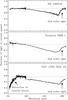 |
Fig. A.1
The ratio of flux in the central spaxel to the flux in the central 3 × 3 spaxels for HD 100546, Serpens SMM 1, and NGC 1333 IRAS 4B. The ratio falls linearly above >100 μm until 190 μm. Second order light contaminates the spectrum at >190. Because the first and second order light have different point-spread functions, the plotted ratio determines the fraction of first and second order photons versus wavelength. For NGC 1333 IRAS 4B, the continuum flux in the central spaxel falls at <70 μm, likely because of extinction. |
| Open with DEXTER | |
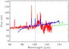 |
Fig. A.2
The first and second order spectrum of IRAS 4B at ~100 μm. The second order light at 100 μm (blue), calibrated from the ~200 μm spectrum, matches the standard first and second order spectra (red and green). The lines in the blue spectrum are artificially weak, by a factor equivalent to the ratio of first to second order light, because the lines and continuum are treated separately. The dotted vertical line shows the location of the CO 13–12 line at 200.27 μm. |
| Open with DEXTER | |
Appendix B: Unidentified lines
All strong lines in the IRAS 4B spectrum are identified. Table B.1 lists several possible lines that are detected at the ~3 σ significance level. The position of several of these tentative detections do not correspond to expected emission lines. Although no o-H O are clearly detected, the o-HO 212 − 110 109.346 μm line is expected to be among the strongest HO lines and is tentatively detected. The centroid of the detected emission is − 170 km s-1 from the expected centroid, based on the measured wavelengths of other nearby lines. Emission is detected consistent with the location of the p-H2O 551 − 624 71.787 μm line, but the line flux is expected to be very weak.
These lines are all very weak and may be statistical fluctuations in the spectrum rather than significant detections of unidentified lines.
Appendix C: Exploring the parameter space in model fits to H2O line fluxes
In Sect. 4, we characterized the physical properties of the H2O emission region by comparing the observed line fluxes to synthetic fluxes calculated in RADEX models of a plane-parallel slab. In this appendix, we describe how the measured line fluxes constrain the parameters of the highly excited gas.
The backbone o-H2O lines 909−818, 818−707, 707 − 616, 616−505, 505−414 and their p-H2O counterparts are amongst the best diagnostics for the excitation and optical depth of the H2O emitting region. The relative flux calibration between these ortho/para pairs should be accurate to better than 5% because the lines are located very near each other. The flux ratio ranges from 2.8–3.5 in the three of the backbone line ratios with highest excitation, indicating that the ortho-to-para ratio of ~3 is thermalized and that these lines are optically-thin. The 616−505, 505 − 414, and 414 − 303 and their p-H2O counterparts have flux ratios of ~2.3−2.5, suggesting that either the modeled emission is moderately optically thick in these lines, or that a second, optically-thick component contributes some emission to the flux in lower-excitation, longer wavelength lines. The top panels of Fig. C.1 show the acceptable space of n(H2) and T for two different values of N(H2O) based on two of these line ratios.
The χ2 statistic automates this type of analysis over all of the applicable lines to find the best-fit parameters for a single isothermal slab. Limiting the χ2 calculation to lines with E′ > 600 K yields two acceptable parameter spaces, one at the H12 location (T ~ 1500 K, log n(H2) ~ 6.5, and log N(H2O) ~ 17.6) and one at low-temperature, high density, and low column density (hereafter X11, with T ~ 200 K, log n(H2) ~ 11, and log N(H2O) ~ 14.0). The X11 parameters differ from W07 because W07 includes a large H2O column density to produce optically thick lines. The X11 parameters are disqualified because several lines, such as o-H2O 330 − 221 66.44 μm, have a synthetic flux that is much stronger than the observed emission8. As a consequence, the χ2 statistic for all lines with E′ > 400 K yields acceptable line fluxes only around the H12 parameters, adopted in this paper, and disqualifies the X11 parameter space.
The o-H2O transitions 550−541 at 75.91 μm and 652 − 643 at 75.83 μm have a 2σ upper limit on the combined flux of 3 × 10-21 W cm-2. Although these upper limits are not included in the χ2 calculations, the non-detections confirm that the parameter space with high H2 density and high H2O column density cannot explain the bulk of the far-IR H2O emission (lower left panel of Fig. C.1). Similarly, the line ratio o-H2O 845 − 734 35.67 μm to o-H2O 707 − 616 71.95 yields physical parameters consistent with the best-fit solution (lower right panel of Fig. C.1).
The non-detection of emission in HO lines (with the possible exception of o-HO 212 − 110 109.35 μm) also places a limit on the opacity of H O lines. The bottom right panel of Fig. C.1 shows where the flux ratio of o-HO 321 − 212 75.87 μm to o-H2O 616 − 505 82.03 μm becomes >50, large enough that the HO line would be detected. This upper limit rules out the parameter space of high density and high column density.
In the H12 model, the strength of the 6 μm continuum emission (Maret et al. 2009) is similar to the strength of the 6 μm rovibrational H2O lines. The non-detection with R = 60 spectra is marginally consistent with the predicted emission and rules out temperatures higher than ~ 2000 K. An AV = 20 mag. would reduce the predicted 6 μm emission by 35%. Decreasing the temperature from 1500 K to 1000 K would reduce the predicted 6 μm emission by a factor of 4.8. Measurements of emission in H2O vibrational lines would place significant additional constraints on the properties of the H2O emission.
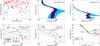 |
Fig. C.1
H2O fluxes and acceptable parameter space of temperature and H2 density. The upper left panel shows that in the H12 model, all far-IR H2O lines expected to be strong are detected (red dots), while those expected to be weak are undetected (black dots). Several lines at ~100 μm were likely undetected because the S/N is degraded in that wavelength region. The upper middle panel shows the acceptable contours for flux ratios of o-H2O 818−707/707−616 (blue), o-H2O 707−616/616−505 (red), and both (purple), for two different column densities. The acceptable parameter space shows the 1σ error bars with a 20% relative flux calibration uncertainty. The lower left panel shows that the non-detection of the o-H2O 550−541 and 652−643 lines relative to o-H2O 616 − 505 line places a limit on the optical depth of the slab. The lower middle panel shows where the flux ratio of o-H2O 845−734 35.669 μm to o-H2O 707−616 71.947 μm is equal to the observed value of 0.07. The lower right panel shows the parameter space (high density and high column density) ruled out by the non-detection of the o-H |
| Open with DEXTER | |
Appendix D: Effect of extinction estimates on rotational diagrams
Extinction can affect the derivation of excitation temperatures and line luminosities, especially at shorter wavelengths where lines typically have upper levels with higher energies. In this analysis, we assume that for all H2O lines, 70% of the luminosity is produced on source behind AV = 700 mag. and 30% is produced off-source at the blueshifted outflow lobe, with AV = 0 mag. (see also Sect. 4.3). This description is consistent with the different observed spatial distributions of the H2O 108.1 and 63.4 μm lines. The excitation conditions and emission line ratios may instead vary smoothly with distance in the outflow.
Applying an extinction correction under these assumptions increases the excitation temperature of the warm (cool) CO component from 850 to 950 K (250 to 280 K). If all the CO emission were located behind the AV = 700 mag., then the temperature difference would become much larger, but the short wavelength CO lines would be very faint. The H2O temperature does not change significantly because the fits are based mostly on lines at short wavelengths, so the emission from the heavily embedded region is mostly extinguished. An AV = 100 mag to the blue outflow lobe would increase the relative luminosity of lines at 25 μm compared with those at 100 μm by a factor of four,
thereby increasing the warm H2O excitation temperature from 220 K to 240 K. An AV > 200 mag to the outflow is ruled out by the significant increase in scatter in the excitation diagram.
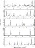 |
Fig. D.1
The continuum-subtracted PACS spectrum of NGC 1333 IRAS 4B from 55–100 μm. The marks identify lines of H2O (blue), CO (red), OH (green), and [O I] (purple). |
| Open with DEXTER | |
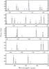 |
Fig. D.2
The continuum-subtracted PACS spectrum of NGC 1333 IRAS 4B from 103–195 μm. The marks identify lines of H2O (blue), CO (red), and OH (green). |
| Open with DEXTER | |
Detected lines in Herschel/PACS spectrum of IRAS 4B.
© ESO, 2012
Current usage metrics show cumulative count of Article Views (full-text article views including HTML views, PDF and ePub downloads, according to the available data) and Abstracts Views on Vision4Press platform.
Data correspond to usage on the plateform after 2015. The current usage metrics is available 48-96 hours after online publication and is updated daily on week days.
Initial download of the metrics may take a while.