| Issue |
A&A
Volume 536, December 2011
Planck early results
|
|
|---|---|---|
| Article Number | A12 | |
| Number of page(s) | 10 | |
| Section | Cosmology (including clusters of galaxies) | |
| DOI | https://doi.org/10.1051/0004-6361/201116489 | |
| Published online | 01 December 2011 | |
Planck early results. XII. Cluster Sunyaev-Zeldovich optical scaling relations⋆
1
Aalto University Metsähovi Radio Observatory, Metsähovintie 114, 02540 Kylmälä, Finland
2
Agenzia Spaziale Italiana Science Data Center, c/o ESRIN, via Galileo Galilei, Frascati, Italy
3
Astroparticule et Cosmologie, CNRS (UMR7164), Université Denis Diderot Paris 7, Bâtiment Condorcet, 10 rue A. Domon et Léonie Duquet, Paris, France
e-mail: This email address is being protected from spambots. You need JavaScript enabled to view it.
4
Astrophysics Group, Cavendish Laboratory, University of Cambridge, J J Thomson Avenue, Cambridge CB3 0HE, UK
5
Atacama Large Millimeter/submillimeter Array, ALMA Santiago Central Offices, Alonso de Cordova 3107, Vitacura, Casilla 763 0355, Santiago, Chile
6
CITA, University of Toronto, 60 St. George St., Toronto, ON M5S 3H8, Canada
7
CNRS, IRAP, 9 Av. colonel Roche, BP 44346, 31028 Toulouse Cedex 4, France
8
California Institute of Technology, Pasadena, California, USA
9 Centre of Mathematics for Applications, University of Oslo, Blindern, Oslo, Norway
10
Centro de Astrofísica, Universidade do Porto, Rua das Estrelas, 4150-762 Porto, Portugal
11
DAMTP, University of Cambridge, Centre for Mathematical Sciences, Wilberforce Road, Cambridge CB3 0WA, UK
12
DSM/Irfu/SPP, CEA-Saclay, 91191 Gif-sur-Yvette Cedex, France
13
DTU Space, National Space Institute, Juliane Mariesvej 30, Copenhagen, Denmark
14
Departamento de Física, Universidad de Oviedo, Avda. Calvo Sotelo s/n, Oviedo, Spain
15
Department of Astronomy and Astrophysics, University of Toronto, 50 Saint George Street, Toronto, Ontario, Canada
16
Department of Physics & Astronomy, University of British Columbia, 6224 Agricultural Road, Vancouver, British Columbia, Canada
17
Department of Physics and Astronomy, University of Southern California, Los Angeles, California, USA
18
Department of Physics, Gustaf Hällströmin katu 2a, University of Helsinki, Helsinki, Finland
19
Department of Physics, Princeton University, Princeton, New Jersey, USA
20
Department of Physics, Purdue University, 525 Northwestern Avenue, West Lafayette, Indiana, USA
21
Department of Physics, University of California, Berkeley, California, USA
22
Department of Physics, University of California, One Shields Avenue, Davis, California, USA
23
Department of Physics, University of California, Santa Barbara, California, USA
24
Department of Physics, University of Illinois at Urbana-Champaign, 1110 West Green Street, Urbana, Illinois, USA
25
Dipartimento di Fisica G. Galilei, Università degli Studi di Padova, via Marzolo 8, 35131 Padova, Italy
26
Dipartimento di Fisica, Università La Sapienza, P. le A. Moro 2, Roma, Italy
27
Dipartimento di Fisica, Università degli Studi di Milano, via Celoria, 16, Milano, Italy
28
Dipartimento di Fisica, Università degli Studi di Trieste, via A. Valerio 2, Trieste, Italy
29
Dipartimento di Fisica, Università di Ferrara, via Saragat 1, 44122 Ferrara, Italy
30
Dipartimento di Fisica, Università di Roma Tor Vergata, via della Ricerca Scientifica 1, Roma, Italy
31
Discovery Center, Niels Bohr Institute, Blegdamsvej 17, Copenhagen, Denmark
32
Dpto. Astrofísica, Universidad de La Laguna (ULL), 38206 La Laguna, Tenerife, Spain
33
European Southern Observatory, ESO Vitacura, Alonso de Cordova 3107, Vitacura, Casilla 19001, Santiago, Chile
34
European Space Agency, ESAC, Planck Science Office, Camino bajo del Castillo, s/n, Urbanización Villafranca del Castillo, Villanueva de la Cañada, Madrid, Spain
35
European Space Agency, ESTEC, Keplerlaan 1, 2201 AZ Noordwijk, The Netherlands
36
GEPI, Observatoire de Paris, Section de Meudon, 5 Place J. Janssen, 92195 Meudon Cedex, France
37
Helsinki Institute of Physics, Gustaf Hällströmin katu 2, University of Helsinki, Helsinki, Finland
38
INAF – Osservatorio Astronomico di Padova, Vicolo dell’Osservatorio 5, Padova, Italy
39
INAF – Osservatorio Astronomico di Roma, via di Frascati 33, Monte Porzio Catone, Italy
40
INAF – Osservatorio Astronomico di Trieste, via G.B. Tiepolo 11, Trieste, Italy
41
INAF/IASF Bologna, via Gobetti 101, Bologna, Italy
42
INAF/IASF Milano, via E. Bassini 15, Milano, Italy
43
INRIA, Laboratoire de Recherche en Informatique, Université Paris-Sud 11, Bâtiment 490, 91405 Orsay Cedex, France
44
IPAG: Institut de Planétologie et d’Astrophysique de Grenoble, Université Joseph Fourier, Grenoble 1/CNRS-INSU, UMR 5274, 38041 Grenoble, France
45
Imperial College London, Astrophysics group, Blackett Laboratory, Prince Consort Road, London, SW7 2AZ, UK
46
Infrared Processing and Analysis Center, California Institute of Technology, Pasadena, CA 91125, USA
47
Institut Néel, CNRS, Université Joseph Fourier Grenoble I, 25 rue des Martyrs, Grenoble, France
48
Institut d’Astrophysique Spatiale, CNRS (UMR8617) Université Paris-Sud 11, Bâtiment 121, Orsay, France
49
Institut d’Astrophysique de Paris, CNRS UMR7095, Université Pierre & Marie Curie, 98 bis boulevard Arago, Paris, France
50
Institute of Astronomy and Astrophysics, Academia Sinica, Taipei, Taiwan
51
Institute of Astronomy, University of Cambridge, Madingley Road, Cambridge CB3 0HA, UK
52 Institute of Theoretical Astrophysics, University of Oslo, Blindern, Oslo, Norway
53
Instituto de Astrofísica de Canarias, C/vía Láctea s/n, La Laguna, Tenerife, Spain
54
Instituto de Física de Cantabria (CSIC-Universidad de Cantabria), Avda. de los Castros s/n, Santander, Spain
55
Jet Propulsion Laboratory, California Institute of Technology, 4800 Oak Grove Drive, Pasadena, California, USA
56
Jodrell Bank Centre for Astrophysics, Alan Turing Building, School of Physics and Astronomy, The University of Manchester, Oxford Road, Manchester, M13 9PL, UK
57
Kavli Institute for Cosmology Cambridge, Madingley Road, Cambridge, CB3 0HA, UK
58
LERMA, CNRS, Observatoire de Paris, 61 Avenue de l’Observatoire, Paris, France
59
Laboratoire AIM, IRFU/Service d’Astrophysique - CEA/DSM - CNRS - Université Paris Diderot, Bât. 709, CEA-Saclay, 91191 Gif-sur-Yvette Cedex, France
60
Laboratoire Traitement et Communication de l’Information, CNRS (UMR 5141) and Télécom ParisTech, 46 rue Barrault, 75634 Paris Cedex 13, France
61
Laboratoire de Physique Subatomique et de Cosmologie, CNRS/IN2P3, Université Joseph Fourier Grenoble I, Institut National Polytechnique de Grenoble, 53 rue des Martyrs, 38026 Grenoble Cedex, France
62
Laboratoire de l’Accélérateur Linéaire, Université Paris-Sud 11, CNRS/IN2P3, Orsay, France
63
Lawrence Berkeley National Laboratory, Berkeley, California, USA
64
Max-Planck-Institut für Astrophysik, Karl-Schwarzschild-Str. 1, 85741 Garching, Germany
65
Max-Planck-Institut für Extraterrestrische Physik, Giessenbachstraße, 85748 Garching, Germany
66
MilliLab, VTT Technical Research Centre of Finland, Tietotie 3, Espoo, Finland
67
National University of Ireland, Department of Experimental Physics, Maynooth, Co. Kildare, Ireland
68
Niels Bohr Institute, Blegdamsvej 17, Copenhagen, Denmark
69
Observational Cosmology, Mail Stop 367-17, California Institute of Technology, Pasadena, CA, 91125, USA
70
Optical Science Laboratory, University College London, Gower Street, London, UK
71
SISSA, Astrophysics Sector, via Bonomea 265, 34136 Trieste, Italy
72
SUPA, Institute for Astronomy, University of Edinburgh, Royal Observatory, Blackford Hill, Edinburgh EH9 3HJ, UK
73
School of Physics and Astronomy, Cardiff University, Queens Buildings, The Parade, Cardiff, CF24 3AA, UK
74
Space Research Institute (IKI), Russian Academy of Sciences, Profsoyuznaya Str, 84/32, Moscow 117997, Russia
75
Space Sciences Laboratory, University of California, Berkeley, California, USA
76
Stanford University, Dept of Physics, Varian Physics Bldg, 382 via Pueblo Mall, Stanford, California, USA
77
Universität Heidelberg, Institut für Theoretische Astrophysik, Albert-Überle-Str. 2, 69120 Heidelberg, Germany
78
Université Denis Diderot (Paris 7), 75205 Paris Cedex 13, France
79
Université de Toulouse, UPS-OMP, IRAP, 31028 Toulouse Cedex 4, France
80
University of Granada, Departamento de Física Teórica y del Cosmos, Facultad de Ciencias, Granada, Spain
81
University of Miami, Knight Physics Building, 1320 Campo Sano Dr., Coral Gables, Florida, USA
82
Warsaw University Observatory, Aleje Ujazdowskie 4, 00-478 Warszawa, Poland
Received: 10 January 2011
Accepted: 25 June 2011
Abstract
We present the Sunyaev-Zeldovich (SZ) signal-to-richness scaling relation (Y500 − N200) for the MaxBCG cluster catalogue. Employing a multi-frequency matched filter on the Planck sky maps, we measure the SZ signal for each cluster by adapting the filter according to weak-lensing calibrated mass-richness relations (N200 − M500). We bin our individual measurements and detect the SZ signal down to the lowest richness systems (N200 = 10) with high significance, achieving a detection of the SZ signal in systems with mass as low as M500 ≈ 5 × 10¹³ M⊙. The observed Y500 − N200 relation is well modeled by a power law over the full richness range. It has a lower normalisation at given N200 than predicted based on X-ray models and published mass-richness relations. An X-ray subsample, however, does conform to the predicted scaling, and model predictions do reproduce the relation between our measured bin-average SZ signal and measured bin-average X-ray luminosities. At fixed richness, we find an intrinsic dispersion in the Y500 − N200 relation of 60% rising to of order 100% at low richness. Thanks to its all-sky coverage, Planck provides observations for more than 13000 MaxBCG clusters and an unprecedented SZ/optical data set, extending the list of known cluster scaling laws to include SZ-optical properties. The data set offers essential clues for models of galaxy formation. Moreover, the lower normalisation of the SZ-mass relation implied by the observed SZ-richness scaling has important consequences for cluster physics and cosmological studies with SZ clusters.
Key words: galaxies: clusters: intracluster medium / cosmic background radiation / large-scale structure of Universe / cosmology: observations / galaxies: clusters: general
Corresponding author: J. G. Bartlett, e-mail: This email address is being protected from spambots. You need JavaScript enabled to view it.
© ESO, 2011
1. Introduction
Galaxy cluster properties follow simple scaling laws (see e.g. Rosati et al. 2002; Voit 2005, for recent reviews). This attests to a remarkable consistency in the cluster population and motivates the use of clusters as cosmological probes. These scaling laws also provide important clues to cluster formation, and relations involving optical properties, in particular, help uncover the processes driving galaxy evolution.
The Sunyaev-Zeldovich (SZ) effect (Sunyaev & Zeldovich 1972; Birkinshaw 1999) opens a fresh perspective on cluster scaling laws, and the advent of large-area SZ surveys furnishes us with a powerful new tool (Carlstrom et al. 2002). Proportional
to ICM mass and temperature, the thermal SZ effect probes the gas in a manner complementary to X-ray measurements, giving a more direct view of the gas mass and energy content. Ground-based instruments, such as the Atacama Cosmology Telescope (ACT, Swetz et al. 2008), the South Pole Telescope (SPT, Carlstrom et al. 2011) and APEX-SZ (Dobbs et al. 2006), are harvesting a substantial crop of scientific results and producing, for the first time, SZ-selected catalogues and using them to constrain cosmological parameters (Staniszewski et al. 2009; Marriage et al. 2011; Sehgal et al. 2011; Vanderlinde et al. 2010; Hand et al. 2011; Williamson et al. 2011).
The Planck1 consortium has published its first scientific results (Planck Collaboration 2011a) and released the Planck Early Release Compact Source Catalogue (ERCSC) (Planck Collaboration 2011c), which includes the Planck early SZ (ESZ) all-sky cluster list (Planck Collaboration 2011d). Planck (Tauber et al. 2010; Planck Collaboration 2011a) is the third generation space mission to measure the anisotropy of the cosmic microwave background (CMB). It observes the sky in nine frequency bands covering 30–857 GHz with high sensitivity and angular resolution from 31′–5′. The Low Frequency Instrument (LFI; Mandolesi et al. 2010; Bersanelli et al. 2010; Mennella et al. 2011) covers the 30, 44, and 70 GHz bands with amplifiers cooled to 20K. The High Frequency Instrument (HFI; Lamarre et al. 2010; Planck HFI Core Team 2011a) covers the 100, 143, 217, 353, 545, and 857 GHz bands with bolometers cooled to 0.1K. Polarization is measured in all but the highest two bands (Leahy et al. 2010; Rosset et al. 2010). A combination of radiative cooling and three mechanical coolers produces the temperatures needed for the detectors and optics (Planck Collaboration 2011b). Two Data Processing Centres (DPCs) check and calibrate the data and make maps of the sky (Planck HFI Core Team 2011b; Zacchei et al. 2011). Planck’s sensitivity, angular resolution, and frequency coverage make it a powerful instrument for galactic and extragalactic astrophysics, as well as cosmology. Early astrophysics results are given in Planck Collaboration (2011d)-Planck Collaboration (2011u).
Planck early results on clusters of galaxies are presented in this paper and in (Planck Collaboration 2011d–g). In the present work, we use Planck SZ measurements at the locations of MaxBCG clusters (Koester et al. 2007a) to extract the SZ signal-richness scaling relation. There are several optical cluster catalogs (Wen et al. 2009; Hao et al. 2010; Szabo et al. 2011) available from the Sloan Digital Sky Survey (York et al. 2000, SDSS). For this initial study, we chose the MaxBCG catalogue for its large sample size, wide mass range and well-characterized selection function, and because its properties have been extensively studied. In particular, we benefit from weak-lensing mass measurements and mass-richness relations (Johnston et al. 2007; Mandelbaum et al. 2008a; Sheldon et al. 2009; Rozo et al. 2009). A combined SZ-optical study over such a large catalogue is unprecedented and Planck is a unique SZ instrument for this task, as its all-sky coverage encompasses the complete SDSS area and the full MaxBCG cluster sample.
Our analysis methodology follows that of the accompanying paper on the SZ properties of X-ray selected clusters (Planck Collaboration 2011f). Although the individual SZ measurements in both cases generally have low signal-to-noise, we extract the statistical properties of the ICM – mean relations and their dispersion – by averaging over the large sample. The approach enables us to study the properties of a much larger and representative sample of clusters than otherwise possible.
The SZ-richness relation adds a new entry to the complement of cluster scaling laws and additional constraints on cluster and galaxy evolution models. With a mass-richness relation, we can also derive the SZ signal-mass relation. This is a central element in predictions for the diffuse SZ power spectrum and SZ cluster counts. Poor knowledge of the relation represents an important source of modeling uncertainty. Low mass systems, for example, contribute a large fraction of the SZ power, but we know very little about their SZ signal.
We organise the paper as follows: the next section presents the data used, both the Planck maps and the MaxBCG catalogue and pertinent characteristics. Section 3 details our SZ measurements based on a multi-frequency matched filter, and outlines some of the systematic checks. In Sect. 4 we present our basic results and in Sect. 5 compare them to model expectations. Section 6 concludes.
1.1. Conventions and notation
In the following, we adopt a flat fiducial cosmology with ΩM = 0.3 with the remainder of the critical density made up by a cosmological constant. We express the Hubble parameter at redshift z as with h = 0.7. Cluster radii are expressed in terms of RΔ, the radius inside of which the mean mass overdensity equals Δ × ρc(z), where ρc(z) = 3H2(z) / 8πG is the critical density at redshift z. Similarly, we quote masses as  . We note that, in contrast, optical cluster studies, and in particular the MaxBCG group, frequently employ radii and masses scaled to the mean matter density, rather than the critical density. For example, it is standard practice to refer to quantities measured within R200b, where the overdensity of 200 is defined with respect to the background density (this corresponds to R60 at z = 0 and R155 at z = 1). For richness we will use the MaxBCG N200, defined as the number of red galaxies with L > 0.4 L ∗ within R200b. Richness N200 is the only quantity in this work defined relative to the mean background density.
We characterize the SZ signal with the Compton-y parameter integrated over a sphere of radius R500 and expressed in arcmin2:  , where DA denotes angular distance, σT is the Thomson cross-section, c the speed of light, me the electron rest mass and P = nekT is the pressure, defined as the product of the electron number density and temperature, k being the Boltzmann constant. The use of this spherical, rather than cylindrical, quantity is possible because we adopt a template SZ profile when using the matched filter (discussed below). We bring our measurements to z = 0 and a fiducial angular distance assuming self-similar scaling in redshift. To this end, we introduce the intrinsic cluster quantity (an “absolute SZ signal strength”)
  , also expressed in arcmin2.
2. Data sets
We base our study on Planck SZ measurements at the positions of clusters in the published MaxBCG cluster catalogue.
2.1. The MaxBCG optical cluster catalogue
The MaxBCG catalogue (Koester et al. 2007b,a) is derived from Data Release 5 (DR5) of the Sloan Digital Sky Survey (York et al. 2000), covering an area of 7500 deg2 in the Northern hemisphere. Galaxy cluster candidates were extracted by color, magnitude and a spatial filter centered on galaxies identified as the brightest cluster galaxy (BCG). The catalogue provides position, redshift, richness and total luminosity for each candidate. In the following we will only use the richness N200, defined as the number of red-sequence galaxies with L > 0.4 L ∗ and within a projected radius at which the cluster interior mean density equals 200 times the mean background density at the redshift of the cluster (see Koester et al. 2007a, for details and the remark in Sect. 1.1). The catalogue consists of 13823 galaxy clusters over the redshift range 0.1 < z < 0.3, with 90% purity and 85% completeness for 10 < N200 < 190 as determined from simulations.
A valuable characteristic for our study is the wide mass range spanned by the catalogue. Another is the fact that numerous authors have studied the catalogue, providing extensive information on its properties. In particular, Sheldon et al. (2009) and Mandelbaum et al. (2008a) have published mass estimates from weak gravitational lensing analyses, which Johnston et al. (2007) and Rozo et al. (2009) use to construct mass-richness (M500 − N200) relations. We apply this relation, as outlined below, to adapt our SZ filter measurements for each individual cluster according to its given richness, N200, as well as in our model predictions.
In their discussion, Rozo et al. (2009) identify the differences between the Sheldon et al. (2009) and Mandelbaum et al. (2008a) mass estimates and the impact on the deduced mass-richness relation. They trace the systematically higher mass estimates of Mandelbaum et al. (2008a) to these authors’ more detailed treatment of photometric redshift uncertainties (Mandelbaum et al. 2008b). Moreover, they note that Johnston et al. (2007), when employing the Sheldon et al. (2009) measurements, used an extended MaxBCG catalogue that includes objects with N200 < 10, where the catalogue is known to be incomplete. These two effects lead Rozo et al. (2009) to propose a flatter mass-richness relation with higher normalisation than the original Johnston et al. (2007) result. In the following, we perform our analysis with both relations; specifically, using the fit in Table 10 for the M500 − N200 relation of Johnston et al. (2007), and Eqs. (4), (A.20) and (A.21) of Rozo et al. (2009).
2.2. Planck data
We use the six HFI channel temperature maps (prior to CMB removal) provided by the DPC and whose characteristics are given in Planck HFI Core Team (2011b). These maps correspond to the observations of intensity in the first ten months of survey by Planck, still allowing complete sky coverage. Hence, they give us access to the entire SDSS survey area and complete MaxBCG catalogue. After masking bad pixels and contaminated regions (e.g., areas where an individual frequency map has a point source at > 10σ), we have Planck observations for 13104 of the 13823 clusters in the MaxBCG catalogue.
3. SZ measurements
We extract the SZ signal at the position of each MaxBCG cluster by applying a multi-frequency matched filter (Herranz et al. 2002; Melin et al. 2006) to the six Planck temperature maps. The technique maximises the signal-to-noise of objects having the known frequency dependence of the thermal SZ effect and the expected angular profile. The filter returns the amplitude of the template, which we then convert into integrated SZ signal, Y500, within R500. It also returns an estimate of the local noise through the filter, σθ500, due to instrumental noise and astrophysical emissions. The same procedure is used in Planck Collaboration (2011f). We refer the reader to Melin et al. (2006, 2011) for details.
3.1. SZ model template
For the filter’s spatial template we adopt the empirical universal pressure profile of Arnaud et al. (2010), deduced from X-ray studies of the REXCESS cluster sample (Böhringer et al. 2007):  (1)where the physical radius r is scaled to x = r / rs, with rs = R500 / c500. For the standard self-similar case (ST case in Appendix B of Arnaud et al. 2010), c500 = 1.156 and the exponents are α = 1.0620, β = 5.4807, γ = 0.3292. The normalisation is arbitrary for purposes of the matched filter. The SZ signal being proportional to the gas pressure, we find the filter template by integrating along the line-of-sight and expressing the result in terms of projected angles: x = θ / θs. We truncate the filter at 5θ500, containing more than 95% of the signal for the model.
3.2. Application of the filter
We apply the matched filter to each cluster in the MaxBCG catalogue, using the mass-richness relation, M500 − N200, to define R500 and set the angular scale θ500 = R500 / DA(z). The filter effectively samples the cluster SZ signal along a cone out to a transverse angular radius of 5θ500, and returns the normalisation for the template. We apply a geometric factor based on the template SZ profile to convert the deduced total SZ signal along the cone to an equivalent Y500 value, the SZ signal integrated within a sphere of physical radius R500. To account for the redshift range of the catalogue, we scale these measurements according to self-similar expectations to redshift z = 0 and a fiducial angular distance of 500 Mpc:  . We accordingly adapt the estimated filter noise σθ500 to uncertainty
  on these scaled SZ signal measurements. The results of this procedure when using the Johnston et al. (2007) mass-richness relation are shown in Fig. 1.
3.3. Systematic effects
As in the other four Planck SZ papers (Planck Collaboration 2011d–g), we have carried out various tests to ensure the robustness of the Planck SZ measurements. They included investigation of the cluster size-flux degeneracy, evaluation of the impact of the assumed pressure profile used for the Planck cluster detection, of beam-shape effects, color corrections, potential contamination by point sources, as well as an overall error budget estimation. We refer the reader to Sect. 6 of Planck Collaboration (2011d) for an extensive description of this common analysis.
To complete this investigation in the present work, we repeated our entire analysis, changing both the instrument beams and adopted SZ profiles. In the former instance, we varied the beams at all frequencies together to the extremes of their associated uncertainties as specified by the DPC (Planck HFI Core Team 2011b). All beams were increased or all decreased in lock-step to maximize any effect. To investigate the profile, we re-extracted the SZ signal using a non-standard SZ signal-mass scaling, and separately for cool-core and morphologically disturbed SZ profiles (based on the work of Arnaud et al. 2010). In all cases, the impact on the measurements was of order a few percent and thus negligibly impacts our conclusions.
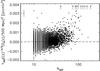 |
Fig.1 Individual scaled SZ signal measurements, |
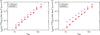 |
Fig.2 Scaled SZ signal measurements, |
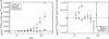 |
Fig.3 Null test performed by randomising the angular positions of the clusters. The red diamonds show the bin-average, redshift-scaled measurements, |
4. Results
Our basic measurements are the set of individual scaled SZ signal values  for each MaxBCG cluster, given as a function of richness N200 in Fig. 1 for the Johnston et al. (2007) mass calibration. At high richness we can detect by eye a slight upturn of the points. Except for the most massive objects, however, the signal-to-noise of the individual measurements is small, in most cases well below unity. This is as expected given the masses of the clusters and the Planck noise levels.
To extract the signal, we bin these values by richness and calculate the bin averages as the noise-weighted mean of all individual i = 1,..,Nb measurements falling within the bin:  . We plot the result as the red diamonds in Fig. 2. The bold error bars represent only the statistical uncertainty associated with the SZ signal measurements:
  (in some cases the error bars are hidden by the size of the data point in the figure). The left-hand panel of the figure shows results using the Johnston et al. (2007) mass calibration, while the right-hand side gives results for the Rozo et al. (2009) mass calibration. The individual SZ signal measurements are not sensitive to this choice: the different calibrations do modify the adopted filter size, but the impact on the measured signal is small.
We quantify the significance of the SZ detection using a null test: we perform an identical analysis on the MaxBCG catalogue after first randomising the cluster angular positions within the SDSS DR5 footprint. In this analysis we are therefore attempting to measure SZ signal with the same set of filters, but now positioned randomly within the SDSS survey. The result is shown in Fig. 3 by the green triangles, to be compared to the actual MaxBCG measurement given by the red diamonds. The left-hand panel presents the null test over the full richness range, while the right-hand panel affords an expanded view of the low mass end. The analysis on the randomised catalog remains consistent with zero (no detection) to within the SZ measurement uncertainty over the entire richness range. The actual measurements of the MaxBCG clusters, on the other hand, deviate by many σ from zero. We reject the null hypothesis in all bins at high significance.
Figure 4 summarises our analysis of the uncertainty and intrinsic scatter as a function of richness. In the left panel we show the uncertainty on the mean signal in each bin, expressed as a fraction of . The red solid red line traces the uncertainty on the mean signal due to just the measurement error, i.e., the noise level in the filter. The blue dashed line gives the uncertainty on the mean assuming that the measurements within a bin are Gaussian distributed about the mean with variance equal to the empirical in-bin variance. We show the relative uncertainty calculated from a bootstrap analysis of the entire catalogue as the dot-dashed, green curve. We perform our full analysis on 10000 bootstrap realisations from the actual catalogue and use the distribution of the resulting bin averages to find the relative uncertainty. The difference between the bootstrap and measurement uncertainties (red line) towards higher richness represents a detection of intrinsic scatter in those bins. At N200 < 30, this difference is small and any intrinsic scatter is difficult to distinguish from the measurement errors.
Scaled Planck SZ signal measurements binned by N200 for the Rozo et al. (2009) mass-richness relation.
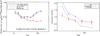 |
Fig.4 Dispersion analysis. Left-hand panel: relative uncertainty on the mean versus richness. The relative uncertainty is expressed as a fraction of the bin-average redshift-scaled SZ signal: |


In the right-hand panel of Fig. 4 we show our estimate of the intrinsic scatter in the scaling relation as a function of richness for N200 > 30. This is expressed as a fraction of the mean, . The dot-dashed, blue line traces the empirical, or raw, dispersion around the average signal of each bin. The three-dot-dashed, green line gives the dispersion corresponding to pure SZ measurement noise. To find the intrinsic scatter, we use the estimator: ![Mathematical equation: \begin{equation} \Sigma^2_{\rm b} = \frac{1}{N_{\rm b}-1}\sum_{i=1}^{N_{\rm b}}\left(\Yscaled(i)-[\Yscaled]_{\rm arith}\right)^2 - \frac{1}{N_{\rm b}}\sum_{i=1}^{N_{\rm b}}\sigscaled^2(i) \end{equation}](/articles/aa/full_html/2011/12/aa16489-11/aa16489-11-eq71.png) (2)where
(2)where ![Mathematical equation: \hbox{$[\Yscaled]_{\rm arith}$}](/articles/aa/full_html/2011/12/aa16489-11/aa16489-11-eq72.png) is the straight arithmetic mean in the bin. In the figure we plot
is the straight arithmetic mean in the bin. In the figure we plot  , with
  being the weighted mean, as above. For this calculation we clip all outliers at > 5σ, where σ is the individual cluster SZ signal error. The final result, especially at low richness, depends on the chosen clipping threshold. The scatter is not Gaussian, as the large fractional intrinsic scatter at low richness suggests. Below N200 ≈ 30, it becomes difficult to draw clear conclusions concerning the scatter, as can be appreciated by the fact that the bootstrap and pure SZ measurement uncertainties begin to overlap in the left-hand panel. For this reason, we only calculate the intrinsic scatter for the five highest richness bins in the right-hand panel.
In conclusion, we detect a signal down to the lowest mass systems in the MaxBCG catalog with high statistical significance. This is the central result of our study. According to the mass calibration from Johnston et al. (2007), we observe the SZ signal in objects of mass as low as M500 = (4 − 5) × 1013 M⊙.
5. Discussion
Figure 2 summarises the central results of our study. There are two notable aspects: firstly, we detect the SZ signal at high significance over the entire mass range; moreover, simple power laws adequately represent the observed scaling relations. Secondly, we see a discrepancy in the  relation relative to expectations based on X-ray models and either the Johnston et al. (2007) or Rozo et al. (2009) mass calibrations.
Fitting a power law of the form  (3)directly to the individual scaled measurements (e.g., Fig. 1), we obtain the results summarised in Table 2. The Rozo et al. (2009) mass calibration assigns a larger mass to the clusters, increasing the filter scale and augmenting the measured SZ signal, which we see as the slightly higher normalisation. These fits are plotted as the dashed lines in Fig. 2. The power laws satisfactorily represent the bin-average trends. The reduced χ2 = 1.16 (13104-2 degrees-of-freedom) in both cases is poor; this reflects the presence of the intrinsic scatter, also evident by the larger uncertainties on the fit from the bootstrap analysis.
The blue stars in Fig. 2 represent the predictions of a model based on the Y500 − M500 relation from Arnaud et al. (2010) and the Johnston et al. (2007) (left) or Rozo et al. (2009) (right) M500 − N200 mean scaling relation. It assumes a self-similar Y500 − M500 scaling relation (STD case) calibrated on X-ray observations of the REXCESS cluster sample (Böhringer et al. 2007). This calibration is also consistent with WMAP observations (Melin et al. 2011) and with the Planck analysis (Planck Collaboration 2011f,g). In each bin we average the model predictions in the same way as the Planck observations: we find the model bin-average redshift-scaled SZ signal as the inverse-error-weighted (pure SZ measurement error) average, assigning each cluster in the bin the same error as the actual observation of that object. Note that in the observation plane  , the model (blue) points change with the mass calibration much more than the measurements.
We see a clear discrepancy between the model and the Planck SZ measurements for both mass calibrations. In the case of the Johnston et al. (2007) mass calibration, the discrepancy manifests as a shift in normalisation that we can characterise by a 25% mass shift at given SZ signal: M − → 0.75M; the slope of the observed relation remains consistent with the self-similar prediction. The Rozo et al. (2009) mass calibration, on the other hand, flattens the mass-richness relation and predicts a shallower power law, as well as a higher normalisation; at N200 = 50 there is a factor of 2 between the predicted and observed amplitudes.
We now discuss some possible explanations for this discrepancy. Weak lensing mass estimates are difficult, and as we have seen there is an important difference in the two mass calibrations. Rozo et al. (2009), building on earlier work by Mandelbaum et al. (2008b), discuss some of the issues when measuring the weak-lensing signal for the MaxBCG catalogue. However, it seems unlikely that the weak-lensing mass calibration would be in error to the extent needed to explain the discrepancy seen in Fig. 2. The discrepancy is in fact larger for the Rozo et al. (2009) result, which should be the more robust mass calibration.
Our model predictions use a series of non-linear, mean relations between observables which in reality have scatter that may also be non-Gaussian. The largest scatter is expected to be in the mass-richness relation. If the scatter is large enough, it could bias the predictions. We have investigated the effect of a 45% log-normal scatter in mass at fixed richness (e.g., Rozo et al. 2009) and of a Poissonian distribution in richness at fixed mass. These are realistic expectations for the degree of scatter in the relations. The effect on the predicted, binned SZ signal is at most 20%, not enough to explain the factor of two discrepancy we see.
Contamination of the MaxBCG catalogue with a fraction, f, of objects that do not contribute an SZ signal (e.g., projection effects in the optical) would bias the measured signal low by about 1 − f. The level of contamination needed to explain the magnitude of the discrepancy with the Rozo et al. (2009) calibration (f ≈ 0.5) seems unlikely. The catalogue is estimated, instead, to be close to 90% pure for N200 > 10. Moreover, contamination would also lower the weak-lensing mass calibration by about 1 − f, at given N200. Since the predicted SZ signal scales as M5 / 3, the model SZ signal would drop by an even larger amount than the observed signal.
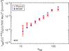 |
Fig.5 The |
To investigate this discrepancy further we analyse, in the same manner, a subsample of the MaxBCG clusters with X-ray data from the MCXC catalogue (Piffaretti et al. 2011). This represents an X-ray detected subsample of the MaxBCG. The results are given in Fig. 5 for the Rozo et al. (2009) mass calibration and with our usual notation. We see that this X-ray subsample, of 189 clusters, matches the model predictions much better. This argues that, at least for this subsample, the weak-lensing mass calibration is not significantly biased. The result also indicates the presence of a range of ICM properties at fixed richness. This is consistent with the study by Rozo et al. (2009), obtained by adapting the approach of Rykoff et al. (2008b), who find a large scatter in X-ray luminosity at fixed N200.
Splitting the catalogue according to the luminosity of the BCG lends support to the presence of populations with different ICM properties. In each bin, we divide the catalogue into a BCG-dominated sample, where the fraction of the cluster luminosity contributed by the BCG is larger than the average for that bin, and its complement sample. The BCG-dominated sample has a notably higher normalisation, closer to the predicted relation, than the complement sample.
We also compare our results to the X-ray results from Rykoff et al. (2008a) who stacked ROSAT photons around MaxBCG clusters according to richness. As with our SZ observations, their individual X-ray fluxes had low signal-to-noise, but they extracted mean luminosities from each image stack (Rykoff et al. 2008b). They report luminosities, L200, over the 0.1 − 2.4 keV band and within R200 for each N200 richness bin. Their analysis revealed a discrepancy between the observed mean luminosities and the X-ray model predictions, using the Johnston et al. (2007) mass calibration.
To compare we re-binned into the same richness bins as Rykoff et al. (2008b), calculating the new, bin-average, redshift-scaled . We also convert their luminosities to L500 using the X-ray profile adopted in Arnaud et al. (2010); the conversion factor is 0.91. In addition, we apply the self-similar redshift luminosity scaling of E − 7 / 3(z = 0.25) to bring the Rykoff et al. (2008a) measurements to equivalent z = 0 values from the values at their median redshift, z = 0.25. The resulting points are shown in Fig. 6.
The model line in the figure is calculated from the z = 0, X-ray luminosities using the X-ray based scaling laws in Arnaud et al. (2010). In this plane the model matches the observations well, demonstrating consistency between the SZ and X-ray observations. Remarkably, the ICM quantities remain in agreement with the model despite the individual discrepancies (SZ and X-ray luminosity) with richness.
The intrinsic scatter in the scaling relation, given in Fig. 4, starts at about 60% and rises to over 100% at N200 ≈ 30. This was calculated by clipping all outliers at > 5σ; the result depends on the choice of clipping threshold, indicative of a non-Gaussian distribution. This dispersion should be compared to the estimated log-normal scatter in the mass-richness relation of  % found by Rozo et al. (2009). Assuming that the dispersion in the SZ signal-mass relation is much smaller, we would expect a dispersion of order 75%, not far from what we find and within the uncertainties. Such large fractional dispersion implies a non-Gaussian distribution skewed toward high SZ signal values, particularly at low richness.
6. Conclusions
We have measured with high significance the mean SZ signal for MaxBCG clusters binned by richness, even the poorest systems. The observed SZ signal-richness relation, based on 13104 of the MaxBCG clusters observed by Planck, is well represented by a power law. This adds another scaling relation to the list of such relations known to exist among cluster properties and that present important constraints on cluster and galaxy evolution models.
The observed relation has a significantly lower amplitude than predicted by X-ray models coupled with the mass-richness relation from weak-lensing observations. The origin of this discrepancy remains unclear. Bias in the weak-lensing mass measurements and/or a high contamination of the catalogue are potential explanations; another would be a bias in hydrostatic X-ray masses relative to weak-lensing based masses (Borgani et al. 2004; Piffaretti & Valdarnini 2008), although the required level of bias would be much larger than expected from simulations. In general, we would expect a wide range of ICM properties at fixed richness (e.g., for example by Rykoff et al. 2008a; Rozo et al. 2009) of which only the more X-ray luminous objects are readily found in X-ray samples used to establish the X-ray model. This is consistent with the better agreement of the model with a subsample of the MaxBCG catalogue with X-ray observations. Remarkably, the relation between mean SZ signal and mean X-ray luminosity for the entire catalogue does conform to model predictions despite discrepant SZ signal-richness and X-ray luminosity-richness relations; properties of the gas halo appear more stably related than either to richness.
We find large intrinsic scatter in the SZ signal-richness relation, although consistent with the major contribution arising from scatter in the mass-richness relation. The uncertainties, however, are important. Such large scatter implies a non-Gaussian distribution of SZ signal at given richness, skewed towards higher signal strengths. This is consistent with the idea of a wide range of ICM properties at fixed richness, with X-ray detected objects preferentially at the high SZ signal end.
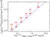 |
Fig.6 Comparison of our bin-average redshift-scaled SZ signal measurements with the mean X-ray luminosities found by Rykoff et al. (2008a). For this comparison, we re-bin into the same bins as Rykoff et al. (2008a) and plot the results as the red diamonds with error bars. The X-ray luminosities are brought to equivalent z = 0 values using the self-similar scaling of E − 7 / 3(z = 0.25) applied at the quoted z = 0.25 median redshift. The dashed blue line shows the predictions of the X-ray model. Our notation for the error bars follows previous figures. The numbers in the figure indicate the number of clusters in each bin. |
The relation, and by consequence the  relation, is an important part of our understanding of the cluster population and a key element in its use as a cosmological probe. Predictions of both the number counts of SZ-detected clusters and the diffuse SZ power spectrum depend sensitively on the relation. The amplitude of the SZ power spectrum varies as the square of the normalisation, while the counts depend on it exponentially. In both instances, this relation represents a significant theoretical uncertainty plaguing models.
Our study of the SZ signal-richness relation is a step towards reducing this uncertainty, and it presents a new cluster scaling relation as a useful constraint for theories of cluster and galaxy evolution. Concerning the latter, we find no obvious sign of an abrupt change in the ICM properties of optically selected clusters over a wide range of richness, hence mass, as might be expected from strong feedback models. Future research with Planck will extend this work to other catalogues and a greater redshift range.
Planck (http://www.esa.int/Planck) is a project of the European Space Agency (ESA) with instruments provided by two scientific consortia funded by ESA member states (in particular the lead countries France and Italy), with contributions from NASA (USA) and telescope reflectors provided by a collaboration between ESA and a scientific consortium led and funded by Denmark.
Acknowledgments
The authors from the consortia funded principally by CNES, CNRS, ASI, NASA, and Danish Natural Research Council acknowledge the use of the pipeline running infrastructures Magique3 at Institut d’Astrophysique de Paris (France), CPAC at Cambridge (UK), and USPDC at IPAC (USA). We acknowledge the use of the HEALPix package (Górski et al. 2005). A description of the Planck Collaboration and a list of its members, indicating which technical or scientific activities they have been involved in, can be found at http://www.rssd.esa.int/Planck.
References
- Arnaud, M., Pratt, G. W., Piffaretti, R., et al. 2010, A&A, 517, A92 [NASA ADS] [CrossRef] [EDP Sciences] [Google Scholar]
- Bersanelli, M., Mandolesi, N., Butler, R. C., et al. 2010, A&A, 520, A4 [NASA ADS] [CrossRef] [EDP Sciences] [Google Scholar]
- Birkinshaw, M. 1999, Phys. Rep., 310, 97 [NASA ADS] [CrossRef] [Google Scholar]
- Böhringer, H., Schuecker, P., Pratt, G. W., et al. 2007, A&A, 469, 363 [NASA ADS] [CrossRef] [EDP Sciences] [Google Scholar]
- Borgani, S., Murante, G., Springel, V., et al. 2004, MNRAS, 348, 1078 [NASA ADS] [CrossRef] [Google Scholar]
- Carlstrom, J. E., Ade, P. A. R., Aird, K. A., et al. 2011, PASP, 123, 568 [NASA ADS] [CrossRef] [Google Scholar]
- Carlstrom, J. E., Holder, G. P., & Reese, E. D. 2002, ARA&A, 40, 643 [NASA ADS] [CrossRef] [Google Scholar]
- Dobbs, M., Halverson, N. W., Ade, P. A. R., et al. 2006, New A Rev., 50, 960 [Google Scholar]
- Górski, K. M., Hivon, E., Banday, A. J., et al. 2005, ApJ, 622, 759 [NASA ADS] [CrossRef] [Google Scholar]
- Hand, N., Appel, J. W., Battaglia, N., et al. 2011, 2011, ApJ, 736, 39 [NASA ADS] [CrossRef] [Google Scholar]
- Hao, J., McKay, T. A., Koester, B. P., et al. 2010, ApJS, 191, 254 [NASA ADS] [CrossRef] [Google Scholar]
- Herranz, D., Sanz, J. L., Hobson, M. P., et al. 2002, MNRAS, 336, 1057 [NASA ADS] [CrossRef] [Google Scholar]
- Johnston, D. E., Sheldon, E. S., Tasitsiomi, A., et al. 2007 [arXiv:0709.1159] [Google Scholar]
- Koester, B. P., McKay, T. A., Annis, J., et al. 2007a, ApJ, 660, 239 [NASA ADS] [CrossRef] [Google Scholar]
- Koester, B. P., McKay, T. A., Annis, J., et al. 2007b, ApJ, 660, 221 [NASA ADS] [CrossRef] [Google Scholar]
- Lamarre, J., Puget, J., Ade, P. A. R., et al. 2010, A&A, 520, A9 [NASA ADS] [CrossRef] [EDP Sciences] [Google Scholar]
- Leahy, J. P., Bersanelli, M., D’Arcangelo, O., et al. 2010, A&A, 520, A8 [NASA ADS] [CrossRef] [EDP Sciences] [Google Scholar]
- Mandelbaum, R., Seljak, U., & Hirata, C. M. 2008a, J. Cosmology Astropart. Phys., 8, 6 [Google Scholar]
- Mandelbaum, R., Seljak, U., Hirata, C. M., et al. 2008b, MNRAS, 386, 781 [NASA ADS] [CrossRef] [Google Scholar]
- Mandolesi, N., Bersanelli, M., Butler, R. C., et al. 2010, A&A, 520, A3 [Google Scholar]
- Marriage, T. A., Acquaviva, V., Ade, P. A. R., et al. 2011, ApJ, 737, 61 [NASA ADS] [CrossRef] [Google Scholar]
- Melin, J., Bartlett, J. G., & Delabrouille, J. 2006, A&A, 459, 341 [NASA ADS] [CrossRef] [EDP Sciences] [Google Scholar]
- Melin, J., Bartlett, J. G., Delabrouille, J., et al. 2011, A&A, 525, A139 [NASA ADS] [CrossRef] [EDP Sciences] [Google Scholar]
- Mennella, A., Butler, R. C., Curto, A., et al. 2011, A&A, 536, A3 [NASA ADS] [CrossRef] [EDP Sciences] [Google Scholar]
- Piffaretti, R., Arnaud, M., Pratt, G. W., Pointecouteau, E., & Melin, J. 2011, A&A, 534, A109 [NASA ADS] [CrossRef] [EDP Sciences] [Google Scholar]
- Piffaretti, R., & Valdarnini, R. 2008, A&A, 491, 71 [NASA ADS] [CrossRef] [EDP Sciences] [Google Scholar]
- Planck Collaboration 2011a, A&A, 536, A1 [NASA ADS] [CrossRef] [EDP Sciences] [Google Scholar]
- Planck Collaboration 2011b, A&A, 536, A2 [NASA ADS] [CrossRef] [EDP Sciences] [Google Scholar]
- Planck Collaboration 2011c, A&A, 536, A7 [NASA ADS] [CrossRef] [EDP Sciences] [Google Scholar]
- Planck Collaboration 2011d, A&A, 536, A8 [NASA ADS] [CrossRef] [EDP Sciences] [Google Scholar]
- Planck Collaboration 2011e, A&A, 536, A9 [NASA ADS] [CrossRef] [EDP Sciences] [Google Scholar]
- Planck Collaboration 2011f, A&A, 536, A10 [NASA ADS] [CrossRef] [EDP Sciences] [Google Scholar]
- Planck Collaboration 2011g, A&A, 536, A11 [NASA ADS] [CrossRef] [EDP Sciences] [Google Scholar]
- Planck Collaboration 2011h, A&A, 536, A12 [NASA ADS] [CrossRef] [EDP Sciences] [Google Scholar]
- Planck Collaboration 2011i, A&A, 536, A13 [NASA ADS] [CrossRef] [EDP Sciences] [Google Scholar]
- Planck Collaboration 2011j, A&A, 536, A14 [NASA ADS] [CrossRef] [EDP Sciences] [Google Scholar]
- Planck Collaboration 2011k, A&A, 536, A15 [NASA ADS] [CrossRef] [EDP Sciences] [Google Scholar]
- Planck Collaboration 2011l, A&A, 536, A16 [NASA ADS] [CrossRef] [EDP Sciences] [Google Scholar]
- Planck Collaboration 2011m, A&A, 536, A17 [NASA ADS] [CrossRef] [EDP Sciences] [Google Scholar]
- Planck Collaboration 2011n, A&A, 536, A18 [NASA ADS] [CrossRef] [EDP Sciences] [Google Scholar]
- Planck Collaboration 2011o, A&A, 536, A19 [NASA ADS] [CrossRef] [EDP Sciences] [Google Scholar]
- Planck Collaboration 2011p, A&A, 536, A20 [NASA ADS] [CrossRef] [EDP Sciences] [Google Scholar]
- Planck Collaboration 2011q, A&A, 536, A21 [NASA ADS] [CrossRef] [EDP Sciences] [Google Scholar]
- Planck Collaboration 2011r, A&A, 536, A22 [NASA ADS] [CrossRef] [EDP Sciences] [Google Scholar]
- Planck Collaboration 2011s, A&A, 536, A23 [NASA ADS] [CrossRef] [EDP Sciences] [Google Scholar]
- Planck Collaboration 2011t, A&A, 536, A24 [Google Scholar]
- Planck Collaboration 2011u, A&A, 536, A25 [NASA ADS] [CrossRef] [EDP Sciences] [Google Scholar]
- Planck Collaboration 2011v, The Explanatory Supplement to the Planck Early Release Compact Source Catalogue (ESA) [Google Scholar]
- Planck Collaboration 2011w, A&A, 536, A26 [NASA ADS] [CrossRef] [EDP Sciences] [Google Scholar]
- Planck HFI Core Team 2011a, A&A, 536, A4 [NASA ADS] [CrossRef] [EDP Sciences] [Google Scholar]
- Planck HFI Core Team 2011b, A&A, 536, A6 [NASA ADS] [CrossRef] [EDP Sciences] [Google Scholar]
- Rosati, P., Borgani, S., & Norman, C. 2002, ARA&A, 40, 539 [NASA ADS] [CrossRef] [Google Scholar]
- Rosset, C., Tristram, M., Ponthieu, N., et al. 2010, A&A, 520, A13 [NASA ADS] [CrossRef] [EDP Sciences] [Google Scholar]
- Rozo, E., Rykoff, E. S., Evrard, A., et al. 2009, ApJ, 699, 768 [NASA ADS] [CrossRef] [Google Scholar]
- Rykoff, E. S., Evrard, A. E., McKay, T. A., et al. 2008a, MNRAS, 387, L28 [NASA ADS] [Google Scholar]
- Rykoff, E. S., McKay, T. A., Becker, M. R., et al. 2008b, ApJ, 675, 1106 [NASA ADS] [CrossRef] [Google Scholar]
- Sehgal, N., Trac, H., Acquaviva, V., et al. 2011, ApJ, 732, 44 [NASA ADS] [CrossRef] [Google Scholar]
- Sheldon, E. S., Johnston, D. E., Scranton, R., et al. 2009, ApJ, 703, 2217 [NASA ADS] [CrossRef] [Google Scholar]
- Staniszewski, Z., Ade, P. A. R., Aird, K. A., et al. 2009, ApJ, 701, 32 [CrossRef] [Google Scholar]
- Sunyaev, R. A., & Zeldovich, Y. B. 1972, Comments on Astrophys. Space Phys., 4, 173 [Google Scholar]
- Swetz, D. S., Ade, P. A. R., Allen, C., et al. 2008, in Presented at the SPIE Conf. Ser., 7020 [Google Scholar]
- Szabo, T., Pierpaoli, E., Dong, F., Pipino, A., & Gunn, J. E. 2011, ApJ, 736, 21 [NASA ADS] [CrossRef] [Google Scholar]
- Tauber, J. A., Mandolesi, N., Puget, J., et al. 2010, A&A, 520, A1 [NASA ADS] [CrossRef] [EDP Sciences] [Google Scholar]
- Vanderlinde, K., Crawford, T. M., de Haan, T., et al. 2010, ApJ, 722, 1180 [NASA ADS] [CrossRef] [Google Scholar]
- Voit, G. M. 2005, Rev. Mod. Phys., 77, 207 [NASA ADS] [CrossRef] [Google Scholar]
- Wen, Z. L., Han, J. L., & Liu, F. S. 2009, ApJS, 183, 197 [NASA ADS] [CrossRef] [Google Scholar]
- Williamson, R., Benson, B. A., High, F. W., et al. 2011, ApJ, 738, 139 [NASA ADS] [CrossRef] [Google Scholar]
- York, D. G., Adelman, J., Anderson, Jr., J. E., et al. 2000, AJ, 120, 1579 [Google Scholar]
- Zacchei, A., Maino, D., Baccigalupi, C., et al. 2011, A&A, 536, A5 [NASA ADS] [CrossRef] [EDP Sciences] [Google Scholar]
All Tables
Scaled Planck SZ signal measurements binned by N200 for the Rozo et al. (2009) mass-richness relation.
All Figures
|
Fig.1 Individual scaled SZ signal measurements, |
| In the text | |
|
Fig.2 Scaled SZ signal measurements, |
| In the text | |
|
Fig.3 Null test performed by randomising the angular positions of the clusters. The red diamonds show the bin-average, redshift-scaled measurements, |
| In the text | |
|
Fig.4 Dispersion analysis. Left-hand panel: relative uncertainty on the mean versus richness. The relative uncertainty is expressed as a fraction of the bin-average redshift-scaled SZ signal: |
| In the text | |
|
Fig.5 The |
| In the text | |
|
Fig.6 Comparison of our bin-average redshift-scaled SZ signal measurements with the mean X-ray luminosities found by Rykoff et al. (2008a). For this comparison, we re-bin into the same bins as Rykoff et al. (2008a) and plot the results as the red diamonds with error bars. The X-ray luminosities are brought to equivalent z = 0 values using the self-similar scaling of E − 7 / 3(z = 0.25) applied at the quoted z = 0.25 median redshift. The dashed blue line shows the predictions of the X-ray model. Our notation for the error bars follows previous figures. The numbers in the figure indicate the number of clusters in each bin. |
| In the text | |
Current usage metrics show cumulative count of Article Views (full-text article views including HTML views, PDF and ePub downloads, according to the available data) and Abstracts Views on Vision4Press platform.
Data correspond to usage on the plateform after 2015. The current usage metrics is available 48-96 hours after online publication and is updated daily on week days.
Initial download of the metrics may take a while.