| Issue |
A&A
Volume 531, July 2011
|
|
|---|---|---|
| Article Number | A136 | |
| Number of page(s) | 20 | |
| Section | Extragalactic astronomy | |
| DOI | https://doi.org/10.1051/0004-6361/201015022 | |
| Published online | 01 July 2011 | |
Chemical evolution of dwarf irregular and blue compact galaxies
1
Key Laboratory for Research in Galaxies and Cosmology, Shanghai
Astronomical Observatory, CAS, 80
Nandan Road, 200030, Shanghai,
PR China
e-mail: This email address is being protected from spambots. You need JavaScript enabled to view it.
2
Department of Physics, Astronomy Division, Trieste
University, via G.B. Tiepolo
11, 34131
Trieste,
Italy
e-mail: This email address is being protected from spambots. You need JavaScript enabled to view it.
3
Osservatorio Astronomico di Trieste, INAF,
via G.B. Tiepolo 11,
34131
Trieste,
Italy
e-mail: This email address is being protected from spambots. You need JavaScript enabled to view it.
Received:
19
May
2010
Accepted:
20
February
2011
Abstract
Aims. Dwarf irregular and blue compact galaxies are very interesting objects since they are relatively simple and unevolved. We aim at deriving the formation and chemical evolution history of late-type dwarf galaxies and at comparing it with DLA systems.
Methods. We present new models for the chemical evolution of these galaxies by assuming different regimes of star formation (bursting and continuous) and different kinds of galactic winds (normal and metal-enhanced). The dark-to-baryonic mass ratio is assumed to be ten in these models. The chemical evolution model follows the evolution of He, C, N, O, S, Si, and Fe in detail. We have collected the most recent data on these galaxies and compared them with our model’s results. We also collected data for damped-Lyman α-systems.
Results. Our results show that in order to reproduce all the properties of these galaxies, including the spread in the chemical abundances, the star formation should have proceeded in bursts and the number of bursts should be not more than ten in each galaxy, and that metal-enhanced galactic winds are required. The presence of metal-enhanced galactic winds can by itself reproduce the observed mass-metallicity relation, although an increasing efficiency of star formation and/or number and/or duration of bursts can also reproduce such a relation equally well.
Conclusions. Metal-enhanced winds, together with an increasing amount of star formation with galactic mass, are required to explain most of the properties of these galaxies. Normal galactic winds, where all the gas is lost at the same rate, do not reproduce the features of these galaxies. On the other hand, a global increase in the amount of star formation (increasing efficiency, number of bursts, or burst duration) with galactic mass is able by itself to reproduce the mass-metallicity relation even without winds, but without metal-enhanced winds is not able to explain many other constraints. We suggest that these galaxies should have suffered a different number of bursts varying from two to ten and that the efficiency of metal-enhanced winds should not have been too high (λmw ~ 1). We predict for these galaxies present-time type Ia SN rates from 0.00084 and 0.0023 per century. Finally, by comparing the abundance patterns of damped Lyman-α objects with our models, we conclude that they are very likely the progenitors of the current dwarf irregulars.
Key words: galaxies: evolution / galaxies: abundances / galaxies: dwarf / galaxies: irregular
© ESO, 2011
1. Introduction
Galaxy formation and evolution is one of the fundamental problems in astrophysics. According to hierarchical clustering models, larger galactic structures develop and grow through the accretion of dwarf galaxies, which are the first structures to collapse and form stars (White & Frenk 1991; Kauffmann et al. 1993). These building-block galaxies are too faint and small to be studied at high redshifts, while a class of nearby metal-deficient dwarf galaxies offer a much better chance of understanding it (Thuan 2008).
Dwarf galaxies, defined arbitrarily as galaxies having an absolute magnitude fainter than MB ~ −18 mag, are the most numerous (about 80–90%) galaxies in the nearby universe (Mateo 1998; Grebel 2001; Karachentsev et al. 2004). It has been suggested that their space density are about 40 times higher than for bright galaxies (Staveley-Smith et al. 1992). Late-type dwarfs, dwarf irregular galaxies (dIrrs), and blue compact dwarf galaxies (BCDs) are galaxies harboring active or recent star formation (SF) activity, but they have low metallicities, large gas content, and mostly young stellar populations. All these features indicate that they are poorly evolved objects, either newly formed galaxies or evolving slowly over the Hubble time. Especially BCDs, the least chemically evolved star-forming galaxies known in the universe (12 + log(O/H) ranging between 7.1 and ~8.4), are excellent laboratories for studying nucleosynthesis processes in a metal-deficient environment, in conditions similar to those prevailing at the time of galaxy formation (Thuan et al. 1995; Izotov & Thuan 1999). The study of the variations of one chemical element compared to another in these poorly evolved star-forming galaxies is crucial for our understanding of the early chemical evolution of galaxies and for constraining models of stellar nucleosynthesis.
DIrrs are dominated by scattered bright Hii regions in the optical, while in Hi they show a complicated fractal-like pattern of shells, filaments, and clumps. Typical Hi masses are ≤109 M⊙.
BCDs are currently undergoing an intense burst of SF, which gives birth to a large number (103−104) of massive stars in a compact region (≤1 kpc), which in turn ionizes the interstellar medium, producing high-excitation supergiant Hii regions and enriching it with heavy elements (Thuan et al. 1995). Part of the extended neutral gas may be kinematically decoupled from the galaxies (van Zee et al. 1998). The majority of BCDs (more than 99%) are not primordial systems, but evolved dwarf galaxies where starburst activity is immersed within an old extended stellar host galaxy (Kunth et al. 1988; Papaderos et al. 1996; Thuan 2008). However, recent work lends strong observational support to the idea that some among the most metal-deficient star-forming galaxies known in the local universe have formed most of their stellar mass within the last 1 Gyr, so they qualify as young galaxy candidates (Papaderos et al. 2002; Izotov & Thuan 2004b; Pustilnik et al. 2004; Aloisi et al. 2007).
Searle et al. (1973) concluded that extremely blue galaxies should have undergone intense bursts of SF separated by long quiescent periods (bursting SF). Recent detections of old underlying stellar populations in most BCDs seem to corroborate their suggestion and reveal at least one other burst of SF besides the present one, even in the case of the most metal-poor BCDs known, I Zw 18 (Östlin 2000) and SBS 0335-052W (Lipovetsky et al. 1999).
Aside from the bursting SF mode, gasping (Tosi et al. 1991) or mild continuous (Carigi et al. 1999; Legrand 2000; Legrand et al. 2000) SF regimes have been proposed for dIrrs and BCDs. The gasping scenario, in which the interburst periods are significantly shorter than the active phases, is probably the more realistic picture for many of them (Schulte-Ladbeck et al. 2001).
It is very likely that dIrrs and BCDs have suffered galactic winds. In the past years, theorists have argued that winds carry heavy elements out of galaxies and that they remove a larger fraction of the metals in lower mass galaxies (Larson 1974; Dekel & Silk 1986; De Young & Gallagher 1990; Mac Low & Ferrara 1999). The observational evidence of outflows from dwarf galaxies has grown rapidly in time (e.g., Meurer et al. 1992; Martin 1996; Bomans et al. 1997). Only recently, however, has it become possible to directly measure the metal content of galactic winds and confirm that winds are indeed metal enhanced (e.g., Martin et al. 2002).
In the previous studies, many models for the chemical evolution of these galaxies appeared and tried to explain the intrinsic spread observed in their properties (Matteucci & Chiosi 1983; Matteucci & Tosi 1985; Pilyugin 1993; Marconi et al. 1994; Bradamante et al. 1998; Henry et al. 2000; Lanfranchi & Matteucci 2003; Romano et al. 2006). Most of these papers suggested that the spread can be reproduced by varying the efficiency of SF or galactic wind from galaxy to galaxy or by assuming that there is self-pollution in the Hii regions where the abundances are measured (Pilyugin 1993). Metal-enhanced winds with different prescriptions were studied (Marconi et al. 1994; Bradamante et al. 1998; Recchi et al. 2001, 2004; Romano et al. 2006).
Besides the chemical abundances, the photometric and spectral properties are also taken into account in some theoretical works (e.g., Vázquez et al. 2003; Stasińska & Izotov 2003; Martín-Manjón et al. 2008, 2009). Martín-Manjón et al. (2008, 2009) combined different codes of chemical evolution, evolutionary population synthesis, and photoionization and concluded that the closed box models with an attenuated bursting SF and an initial SF efficiency (SFE) ϵ = 0.1 ~ 0.3 can reproduce the observed abundances, diagnostic diagrams, and equivalent width-color relations of local H ii galaxies.
In this work, we present a new series of chemical evolution models for dIrrs and BCDs. The models are based on the original one of Bradamante et al. (1998), but consider a larger number of chemical species and updated stellar yields. We tested both the bursting and the continuous regimes of SF By comparing our model results with the most recent data of dIrrs and damped Lyman-α systems (DLAs), we aim at understanding the importance of galactic winds, the history of SF, and the origin of the mass-metallicity relation in dwarf irregulars. A comparison between the properties of local dIrrs and those of high-redshift DLAs will allow us to understand the nature of DLAs and establish whether they can be considered as the progenitors of local dIrrs and BCDs. Moreover, by studying the abundance patterns in detail such as [X/Fe] versus [Fe/H] will allow us to understand if these dwarf galaxies can be the building blocks of more massive galaxies, as suggested by the hierarchical clustering scenario of galaxy formation.
This paper is organized as follows. In Sect. 2, we present the observational constraints. In Sect. 3, the adopted chemical evolution models are described. Our model results are presented in detail in Sect. 4 and discussed in Sect. 5.
2. Observational properties
The metallicity, defined as the fraction of elements other than hydrogen and helium by mass, is an important indicator of the formation and evolutionary stage of a galaxy, and usually correlates with macroscopic properties of late-type galaxies, e.g. luminosity, mass, gas fraction, rotation speed, morphological type (e.g., Garnett 2002; Pilyugin et al. 2004; Lee et al. 2006; Vaduvescu et al. 2007). Except for hydrogen and helium, oxygen is the most abundant element in the universe, and easily measured in Hii regions because of its bright emission lines. In practice, the oxygen abundance is usually used to represent the metallicity of the galaxy.
2.1. Luminosity-metallicity (L – Z) relation and mass-metallicity (M – Z) relation
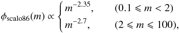
The strong correlation between the metallicity Z and the luminosity L of a galaxy is a robust relationship, maintaining over 10 mag in galaxy optical luminosity and a factor of 100 in metallicity (e.g., Garnett & Shields 1987; Zaritsky et al. 1994; Lamareille et al. 2004; Tremonti et al. 2004). Lequeux et al. (1979) first showed first the correlation between metallicity and mass in both compact and irregular galaxies, which was then confirmed by Skillman et al. (1989), who found that more luminous (or more massive) galaxies are more metal rich. The correlation is also found in spirals and elliptical galaxies (e.g., Garnett & Shields 1987; Brodie & Huchra 1991; Zaritsky et al. 1994; van Zee et al. 1997; Tremonti et al. 2004; Lee et al. 2006; Vaduvescu et al. 2007). Since the luminosity of a galaxy closely relates to its stellar mass, the L − Z relation should also represent the mass-metallicity relation. But how the luminosity is representative of stellar mass depends on the frequency band one investigates. Traditionally, the L − Z relation is studied at optical wavelengths (e.g., Lequeux et al. 1979; Skillman et al. 1989, 1997; Pilyugin 2001; Garnett 2002; Lee et al. 2003a,b; Pilyugin et al. 2004; van Zee & Haynes 2006; Ekta & Chengalur 2010). The optical luminosity could be affected by the current SF process, therefore more and more effort is put into determining the near-infrared L − Z (hence M∗ − Z) relation where the dominant emission arises from the older stellar populations (e.g., Pérez-González et al. 2003; Lee et al. 2004; Salzer et al. 2005; Lee et al. 2006; Mendes de Oliveira et al. 2006; Rosenberg et al. 2006; Vaduvescu et al. 2007; Saviane et al. 2008). Lee et al. (2006) considered 27 nearby star-forming dwarf irregular galaxies whose masses spread over 3 dex, and examined the M∗ − Z relation at 4.5 μm (Spitzer) (see Fig. 1). Vaduvescu et al. (2005, 2006, 2007) studied the properties of both dIrrs and BCDs and obtain the M∗ − Z relation by assuming M∗/LK = 0.8 M⊙/LK ⊙ . They concluded that, for both dIrrs and BCDs, metallicity correlates with stellar mass, gas mass, and baryonic mass, in the sense that more massive systems are more metal-rich.
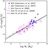 |
Fig. 1 Oxygen abundance vs. stellar mass for nearby dIrrs and BCDs. Filled blue and open magenta circles are data from Vaduvescu et al. (2007), and they represent BCDs and dIrrs, respectively; open magenta triangles are dIrrs observed by Lee et al. (2006), and the dashed line shows the best fit of their data. The solid line is the best linear fit of all the data. |
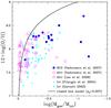 |
Fig. 2 Oxygen abundance vs. gas fraction relation for nearby dIrrs and BCDs. Filled blue and open magenta circles are data from Vaduvescu et al. (2007), and they represent BCDs and dIrrs respectively; open magenta triangles are dIrrs observed by Lee et al. (2006); filled cyan triangles and squares are the Irrs observed by Pilyugin et al. (2004) and Garnett (2002), respectively. The solid line shows the prediction of the closed box model (Z = yZlnμ-1) with an effective yield yZ = 0.007 corresponding to the Salpeter IMF and Woosley & Weaver (1995) nucleosynthesis. |
2.2. Gas fraction-metallicity (μ – Z) relation
A more useful relation for chemical evolution studies is the metallicity-gas fraction (μ − Z) relation, because it provides the information about how the gas convert into stars and metals, and also about gas flows (infall and/or outflow), as first suggested by Matteucci & Chiosi (1983) in their chemical evolution models of dwarf irregular galaxies.
As former works have shown, if the system does not have gas flows, the metallicity evolution predicted by the closed box model is a simple function of the gas fraction μ and true yield y under the instantaneous recycling assumptions, Z = yZln(μ-1) (Schmidt 1963; Searle & Sargent 1972). By comparing the “observed” effective yield, 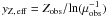 with the true measured yield yZ, one can understand whether the system evolved as a closed box or if infall and/or outflow were important. In fact, both infall and outflow have the effect of decreasing the effective yield.
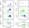 |
Fig. 3 Abundance ratio of different elements. Open blue circles are BCDs, from Izotov & Thuan (1999) and Papaderos et al. (2006); open green squares are DLAs, the data are shown in Table 1. |
Lee et al. (2003a,b) show that the oxygen abundance is tightly correlated with the gas fraction in dwarf irregular galaxies through optical observations, and they argue that these dIrrs have evolved in relative isolation, without inflow or outflow of gas. Later, Lee et al. (2006) measured the 4.5 μm luminosities for 27 nearby dIrrs with the Spitzer Infrared Array Camera, and show the relation between oxygen abundances and the gas-to-stellar mass ratio. Their results suggest reduced yields and/or significant outflow rates, which have also been indicated by previous authors (e.g., Garnett 2002; van Zee & Haynes 2006). Using NIR photometry, the most important discovery of Vaduvescu et al. (2007) is that the μ − Z relation for BCDs follows that of dIrrs, and agrees with Lee et al. (2003a,b) that the evolution of field dIrrs has not been noticeably influenced by gas flows. However, they also point out that several dIrrs and at least one BCD do show HI deficiencies in dense environments, indicating that the gas may be removed by external processes. Using the effective yield as the only criterion for gas flow is too simplistic, so the conclusion might not be reliable. Convincing conclusions should be reached through detailed modeling work.
In Fig. 2, we show the observed oxygen abundance-gas fraction relation of nearby dIrrs and BCDs. From this figure we can see, the BCDs have a broader abundance and gas fraction range, while most dIrrs have a higher gas fraction compared with BCDs and Irrs, implying their poorly evolved stages.
2.3. Abundance ratios
How the abundances of chemical elements change relative to one another is crucial for understanding the chemical evolution of galaxies and stellar nucleosynthesis. Hii regions are ionized by newly born massive stars, hence showing the metallicity of the ISM at the present time; therefore, metallicities in dIrrs and BCDs are usually derived from the ionized gas in Hii regions through their strong narrow emission lines. Izotov & Thuan (1999) present high-quality ground-based spectroscopic observations of 54 supergiant Hii regions in 50 low-metallicity BCDs with oxygen abundances 12 + log(O/H) between 7.1 and 8.3, and determined abundances for the elements N, O, Ne, S, Ar, Fe, and also C and Si in a subsample of seven BCDs. Papaderos et al. (2006) present spectroscopic and photometric studies of nearby BCDs in the 2dFGRS (Two-degree Field Galaxy Redshift Survey), and measured their Ne/O, Fe/O, and Ar/O ratios. Both of these works do not consider the dust depletion correction. We show the data of Izotov & Thuan (1999) and Papaderos et al. (2006) in Fig. 3.
DLA absorption systems, found in the spectra of high-redshift QSOs, are neutral clouds with high Hi column densities, N(HI) ≥ 2 × 1020 cm-2. They are likely to be protogalactic clumps embedded in dark matter halos and may provide important information on the early chemical evolution of galaxies. With high-resolution spectroscopy of QSO absorption lines, elemental abundances can be measured up to redshift z ≈ 5. The chemical abundances of DLA systems give us complementary observational constraints on the formation and evolution of galaxies. Abundance measurements in DLA systems relevant to the present work are listed in Table 1 and plotted in Fig. 3. In comparing DLA abundances with model predictions care must be taken for dust depletion effects. Luckily, these effects are expected to be negligible for most of the elements used in the present investigation, such as C, N, O, and S; in fact, these elements show little depletion, if any, in nearby interstellar clouds (Jenkins 2009) and are expected to even be less depleted in DLA systems. On the other hand, we expect some depletion effects for Fe and, to a lesser extent, for Si. Estimates of Fe depletion in DLAs based on the comparison with Zn measurements (Vladilo 2004) are only available for a few systems of Table 1. These results indicate that Fe tends to be underestimated when the level of metallicity is relatively high. This explains the few cases with largest deviations from BCD measurements and from the model predictions shown in Figs. 3, 5, 8, 10, 11, 13, and 17.
The abundances of DLAs.
2.4. Primordial helium abundance Yp and △ Y/ △ Z
The determination of primordial helium abundance, Yp, is important for the study of cosmology and the evolution of galaxies, because an accurate initial Y is required to test Big Bang nucleosynthesis and build chemical evolution models. One way of estimating Yp is by extrapolating the observed helium-metallicity (Y − Z) relation to Z = 0 by assuming the slope △ Y/ △ Z to be constant. More recently, it has been common practice to use △ Y/ △ O since the oxygen abundance is easier to determine and can represent the metals. To obtain an accurate Yp value, a reliable determination of △ Y/ △ O for oxygen-poor objects is needed (e.g., Izotov et al. 1999; Peimbert 2003; Luridiana et al. 2003; Izotov & Thuan 2004a; Peimbert 2007). Izotov & Thuan (2004a) derived the primordial helium Yp = 0.2429 ± 0.0009 and the slope △ Y/ △ O = 4.3 ± 0.7 from observations of 82 Hii regions. For a restricted sample (7 Hii regions), they obtain Yp = 0.2421 ± 0.0021 and △ Y/ △ O = 5.7 ± 1.8. Later, Izotov et al. (2006) derived Yp = 0.2463 ± 0.0030 from the emission of the whole Hii region of the extremely metal-deficient blue compact dwarf galaxy SBS 0335−052E. Peimbert (2007) has adopted △ Y/ △ O = 3.3 ± 0.7 from theoretical and observational results, and derived Yp = 0.2474 ± 0.0029. These values are in excellent agreement with the value derived by Spergel et al. (2007) from the WMAP results, Yp = 0.2482 ± 0.0004.
In Fig. 4 we replot the helium-oxygen abundance relation of Izotov & Thuan (2004a) by using their data in Table 5. The linear regression is the one derived from the whole sample Y = 0.2429 + 43 ∗ (O/H).
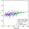 |
Fig. 4 Helium-metallicity (Y − Z) relation for Hii regions in BCDs, Fig. 2 of Izotov & Thuan (2004a). Filled green circles, from Izotov & Thuan (2004a); open red circles, from Izotov & Thuan (1998b); open blue triangles, from Izotov et al. (1997); open magenta pentagrams, from other data (Izotov & Thuan 1998a; Izotov et al. 1999; Thuan et al. 1999; Izotov et al. 2001a,b; Guseva et al. 2001, 2003a,b); the solid line is the maximum likelihood linear regression of all the data, Y = 0.2429 + 43 ∗ (O/H). |
3. Model prescriptions
In this work, we used an updated version of the chemical evolution model developed by Bradamante et al. (1998) to study the formation and evolution of late-type dwarf galaxies, dIrrs and BCDs. The general picture is the following.
Our model is one-zone and assumes the galaxy was built up by continuous infall of primordial gas (X = 0.7571, Yp = 0.2429, Z = 0). Stars form and then contaminate the interstellar medium (ISM) with their newly produced elements, which mix with the ISM instantaneously and completely. Stellar lifetimes are taken into account in detail; i.e., the instantaneous recycling approximation (IRA) is relaxed. The energy released by supernovae (SNe) and stellar winds is partially deposited in the ISM, and galactic winds develop when the thermal energy of the gas exceeds its binding energy. The wind expels metals from the galaxy, making it have a significant influence on the chemical enrichment of the galaxy.
The time evolution of the fractional mass of the element i in the gas, Gi, is described by the equations  (1)where Gi(t) = Mg(t)Xi(t)/ML(tG) is the gas mass in the form of an element i normalized to the total baryonic mass ML at the present day tG = 13 Gyr, Mg(t) is the gas mass at time t, and Xi(t) represents the mass fraction of element i in the gas, i.e., abundance by mass. The quantity G(t) = Mg(t)/ML(tG) represents the total fractional mass of gas and Xi(t) can be expressed by Gi(t)/G(t). The four items on the righthand side of Eq. (1) show the mass change of the element i caused by the formation of new stars ψ(t)Xi(t), the material returned through stellar winds or SN explosion Ri(t), the infall of primordial gas Ġi, inf(t), and the outflow Ġi, out(t), respectively.
The star formation rate (SFR) ψ(t) in this work is simply assumed to be  (2)where ϵ is the SF efficiency and is in units of Gyr-1, one of the free parameters in our work.
Parameters of models without outflow.
The rate of gas infall is assumed to be exponentially decreasing with time:  (3)where A is the normalization constant, which is constrained by the boundary condition
  , and τ is the infall timescale. We can easily obtain the accretion rate of an element i through the formula
  (4)Xi, inf = 0 (i ≠ H, He) if primordial gas is assumed.
In our model, the galactic wind develops when the thermal energy of the gas  exceeds its binding energy
  :
:  (5)The thermal energy of the gas is produced by SN explosions (both type II and type Ia) and stellar winds:
  (6)However, not all the energy produced in these events is stored in the ISM, since a fraction of it is lost by cooling. In Bradamante et al. (1998), the efficiencies of energy transfer from SN and stellar winds into the ISM are the same, ηSNII = ηSNIa = ηsw = 0.03 (see their work for more details). However, more recently, Recchi et al. (2001) and Recchi et al. (2002) have shown that, since SN Ia explosions occur in a hotter and more rarefied medium, their energy can be more efficiently thermalized into the ISM, and consequently, their efficiency of energy transfer is higher. Therefore, in this work we assume that the efficiencies of energy transfer are ηSNII = 0.03,ηSNIa = 0.8, and ηsw = 0.03 for SN II, SN Ia, and stellar winds, respectively.
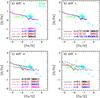 |
Fig. 5 The evolutionary tracks of [O/Fe] vs. [Fe/H] as predicted by models without outflow. a) Models with different number of bursts; b) models with different occurrence times of bursts; c) models with different durations of bursts; d) models with different SFE. All these models assume the same total infall mass Minf = 109 M⊙. The open cyan circles are BCDs and open green squares are DLAs, as in Fig. 3. |
To compute  , the binding energy of gas, we also followed Bradamante et al. (1998) and assumed that each galaxy has a dark matter halo. The binding energy of gas is described as
  (7)with
  (8)which is the potential well due to the luminous matter, and with
  (9)which represents the potential well due to the interaction between dark and luminous matter, where
  , with S = rL/rD, the ratio between the galaxy effective radius (rL) and the radius of the dark matter core (rLD) (see Bertin et al. 1992). As in Bradamante et al. (1998) we assumed that the dark matter halo is ten times more massive than the luminous matter and that S = 0.3.
The rate of gas loss via galactic wind for each element is assumed to be simply proportional to the amount of gas present at the time t:  (10)where Xi, out(t), the abundance of the element i in the wind, is assumed to be same with Xi(t), the abundance in the ISM; λ describes the efficiency of the galactic wind and has the same units as ϵ (Gyr-1); wi is the efficiency weight of each element, hence wiλ is the effective wind efficiency of the element i. Both λ and wi are the other two free parameters in our model. In this work, we have studied two kinds of winds, the normal wind and the metal-enhanced wind. In the case of the normal wind (wind efficiency is denoted by λw), all elements are lost in the same way, i.e., wi = 1 for all elements. However, wind provoked by SN explosions could carry more metals out than H and He (wi > wH,He, i ≠ H,He), which is the so-called “metal-enhanced” wind (Mac Low & Ferrara 1999; Recchi et al. 2001; Fujita et al. 2003; Recchi et al. 2008), and its wind efficiency is denoted by λmw.
The initial mass function (IMF) is usually assumed to be constant both in space and time in different galaxies, and it can be expressed as a power law of stellar mass as suggested first by Salpeter (1955):  (11)where x = 1.35 for Salpeter IMF, and φ0 is the normalization constant, which can be obtained by satisfying ∫mφ(m)dm = 1 in the mass range 0.1−100 M⊙. However, we also tested the Scalo (1986) IMF:
 (12)which is a two-slope IMF and is steeper at the high-mass end.
Stellar yields of different elements are important ingredients in chemical evolution studies. We have adopted stellar yields of Woosley & Weaver (1995) for massive stars and van den Hoek & Groenewegen (1997) for low- and intermediate-mass stars. Both of them are metallicity dependent.
4. Model results
To understand the observed global properties and abundance patterns of late-type dwarf galaxies, we calculated several models. The typical galaxy is assumed to be forming by continuous infall of primordial gas and bursting SF, as suggested by several previous works (e.g., Searle et al. 1973; Matteucci & Chiosi 1983; Marconi et al. 1994; Bradamante et al. 1998; Lanfranchi & Matteucci 2003; Romano et al. 2006). We also checked the case of continuous SF for these galaxies (see Sect. 4.5).
4.1. Model without outflow
Here we examine the models without outflow. Different numbers n, durations d, middle times of the bursts t, and different SFEs ϵ have been tested. The parameters adopted in the models are listed in Table 2. All the models assume short infall timescales (τ = 1 Gyr) except model M9tau, and the galactic lifetime is taken to be 13 Gyr for all the models. From the second to the fourth columns, there are the model names, classified by different total infalling mass, from 108 M⊙ to 1010 M⊙; the fifth column shows the SFE; the sixth column the number of the bursts; the seventh column the middle time of each burst; the eighth column the duration of each burst, where “0.1*3” means that the duration of three bursts are the same, namely 0.1 Gyr.
In Fig. 5, we show the evolutionary tracks of [O/Fe] vs. [Fe/H] as predicted by models with a different number of bursts(panel a), different times for the bursts(panel b), different burst durations (panel c), and also different SFEs (panel d). The most distinctive feature of the bursting SF scenario is the “saw-tooth” behavior of the tracks, which is caused by the different origins of α-elements and iron-peak elements. Oxygen is mainly synthesized by massive stars, therefore its abundance only increases during the bursting time, whereas iron is mainly synthesized by the Type Ia supernovae and its abundance still increases after the burst is over owing to the time delay of SN Ia explosions.
As we can see from Fig. 5, different durations of bursts and different SFEs among galaxies could explain of the scatter in the data. In panel c, as a comparison, we also plot the model results for a low continuous SF process (model M9d4). Clearly in this case the saw-tooth behavior disappears.
If we compare the present oxygen abundance vs. the gas fraction as predicted by the above models with the observations (Fig. 6, upper panel), we can see that, no matter how the star formation history (SFH) changes (different n,t,d,ϵ), the model results always stay along the same curve. As first suggested by Matteucci & Chiosi (1983), to explain the spread in this diagram one should claim a variation in the IMF, in the wind rate, or in the infall rate. Therefore, we examined the other IMF (Scalo 1986) which is steeper than Salpeter IMF at the massive end. However, the model results in Fig. 6 still cannot explain the observed lowest oxygen abundance at the same μ or the lowest μ at the same oxygen abundance. Therefore, unless one assumes unrealistically steeper IMFs, the observed μ − Z strongly implies that there should be other mechanisms operating in the galaxy that can reduce the O abundance or the gas fraction.
The lower panel of Fig. 6 shows the Y − (O/H) relation as predicted by our model, which is consistent with the observations, although a little flatter than the observed best fit. The best fit to these model results is Y = 0.2428 + 12.07(O/H).
Since we assume a linear correlation between SFR and gas, the models with different total infalling masses are self-similar; therefore, when the abundance ratios and gas fraction are examined (Figs. 5 and 6), the three series of models (M8, M9, and M10) overlap.
In Fig. 7 we plot the mass-metallicity relations predicted by models without wind. We ran models for three different infall masses (108, 109, 1010 M⊙). The effects of different numbers of bursts (n = 1,3,7), different durations (d = 0.03,0.1,0.3), and different SFEs (ϵ = 0.2,0.5,1.0,2.0) as functions of galactic mass are shown. It is evident from Fig. 7 that our models can reproduce the M − Z relation very well even without the galactic wind, just by assuming an increase in the number, duration of bursts, or the efficiency of SF.
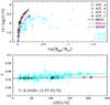 |
Fig. 6 Present oxygen abundance vs. gas fraction (upper panel) and Y vs. oxygen abundance (lower panel) as predicted by models without wind. All these models assume the same total infall mass Minf = 109 M⊙. Big open black circles: models with different numbers of bursts; big open black triangles: models with different durations of bursts; big open black squares: models with different occurrence times of bursts; big open black pentacles: models with different SFE. Solid black, dotted red and dashed blue lines in the upper panel are the evolutionary tracks of model M9d4, M9tau and M9IMF. The solid black line in the lower panel is the best fit of all the model points. The observational data are the same as in Figs. 2 and 4, open cyan circles and open cyan triangles represent BCDs and dIrrs, respectively. The solid cyan line is the best fit of the observational data. |
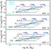 |
Fig. 7 Present-day oxygen abundance vs. M∗ as predicted by models without wind. The upper (middle/lower) panel shows the model results with different numbers of bursts (durations/SFE), along the dashed blue lines the number of bursts (durations/SFE) increases from 2 to 7 (0.02 to 0.3/ 0.1 to 2), and along the solid black lines the total infall mass Minf increases from 108 to 1010 M⊙. The thick solid red line connects the models that are consistent with the observational data, larger n (d/ϵ) for more massive galaxy. The observational data are the same as in Fig. 1, open cyan circles for BCDs and open cyan triangles for dIrrs. |
4.2. Model with normal wind
If the galactic wind has the same chemical composition as the well-mixed ISM, i.e., wi = 1 for all the elements, we call it “normal wind”. In Fig. 8, we show the evolutionary tracks predicted by models with normal wind; abundance ratios of log(C/O) vs. 12 + log(O/H) and [O/Fe] vs. [Fe/H] are on the lefthand side, while μ − Z and Y − Z relations are on the right. The models have the same total infall mass (Minf = 109 M⊙), the same burst sequence (t = 1/3/5/7/9/11/13 Gyr, with d = 0.1 Gyr for each burst), but different wind efficiencies (λw = 0,0.2,0.5,1.0). Oxygen is produced by massive stars, therefore no oxygen will be ejected into the ISM after SF ceases. On the other hand, elements, such as C and N produced by low- and intermediate-mass stars and Fe mainly produced by SN Ia explosion, are continuously polluting the ISM after the SF stops, owing to their long lifetimes. Therefore, the decrease in the mass of gas (i.e., H and He) and the α-elements lost with the wind will result in a dramatic increase in the abundance of the “time-delayed” elements. The stronger the wind, the higher the abundance of C or Fe compared to the O predicted by the models.
The main effect of normal winds is to decrease the gas fraction with a weaken effect on the O/H abundance, as we can see from the 12 + log(O/H)-μ relation (upper right panel of Fig. 8). This means that models with a normal wind cannot explain the whole spread in O/H observed at a given μ for these galaxies. There are two possible reasons for that. One is the same wind efficiency (i.e., wiλw) for both O and H in the normal wind, so that both O and H decrease at the same time. The other one is the short infall time scale assumed (τ = 1 Gyr). In this case, no primordial gas falls into the galaxies to dilute the ISM at late evolutionary times. Therefore, we also developed a model with long infall timescale (τ = 10 Gyr, Fig. 8). It is clear that in this model the metallicity decreases in the interburst time. Actually, the infall of primordial gas (i.e., H and He) results in a lower mass loss rate for H and He than for metals, similar to the metal-enhanced wind case discussed in the next section. A very strong normal wind (e.g. λw > 0.5) seems unlikely in late-type dwarf galaxies since it would lose a large amount of gas, so would predict too low a gas fraction, as is evident in Fig. 8. In the lower right panel of Fig. 8, the predicted Y vs. (O/H) relation is shown to be consistent with the observational data at the low metallicity, because the wind has not developed yet when the galaxy is still very metal poor. However, after the wind, an increase in the He abundance, as well as of the abundances of elements produced on long timescale occurs, especially in the case of a strong wind that produces a very low final gas fraction.
In the proceeding section, we pointed out that the observed M − Z relation could indicate more star bursts or longer duration for each burst or higher SFE in more massive galaxies, if no outflow takes place. Now we examine the possibility of the normal wind being the explanation of the M − Z relation, as suggested by many previous authors. In Fig. 9, we take the models with seven bursts for example (i.e., Model M8n4, M9n4, M10n4 in no-wind case) but different strengths of normal wind are introduced (λw = 0,0.2,0.5,1,3). It is evident from the upper panel of Fig. 9 that by varying only the efficiency of a normal wind one cannot reproduce the M − Z relation, unless other parameters, such as the efficiency of SF or the number of bursts, are assumed to vary as functions of the galactic mass. When a long infall timescale is adopted (τ = 10 Gyr, lower panel of Fig. 9), fewer stars are formed in each model due to the slow gas accretion process, and the wind could not be induced in the high-mass systems (Minf ≈ 1010 M⊙). However in the low-mass galaxy (Minf = 108 M⊙), where the wind could develop, the newly infalling gas dilutes the ISM effectively. Therefore, the general trend of the M − Z relation could be reproduced by combining the normal wind with a slow accretion process.
In summary, the normal wind can strongly reduce the gas fraction but it cannot noticeably reduce the O/H. To explain the spread observed in O/H at the same μ, we should invoke other mechanisms, such as a continuous supplement of primordial gas or a metal-enhanced wind (see Sect. 4.3), both of which imply a lower mass loss rate for H and He than for metals.
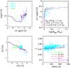 |
Fig. 8 The evolutionary track as predicted by models with normal wind. The left two panels are log(C/O) vs. 12 + log(O/H) and [O/Fe] vs. [Fe/H]; the right two panels are oxygen abundance vs. gas fraction and Y vs. (O/H). All the 5 models have the same bursts sequence (τ = 1 Gyr, t = 1/3/5/7/9/11/13 Gyr, and d = 0.1 Gyr for each burst), but different wind efficiencies, solid green lines for λm = 0, dash-dotted black lines for λm = 0.2, long-dashed red lines for λm = 0.5, and short-dashed blue lines for λm = 1. A model with long infall timescale (τ = 10 Gyr, λm = 1) is shown in magenta dotted line. All these models assume the same total infall mass Minf = 109 M⊙. The observational data are the same as in Figs. 2–4, BCDs, dIrrs, and DLAs are plotted in open cyan circles, open cyan triangles and open green squares here. |
4.3. Model with metal-enhanced wind
The galactic wind, mainly induced by SN explosion, could blow the metal-enriched gas out of the galaxy, which means metals are lost more efficiently than the gas (H and He). We define the wind “metal-enhanced” when the abundances of metals it carries out are higher than in the ISM. Metal-enhanced winds have been already suggested by several dynamical works (e.g. Mac Low & Ferrara 1999; Recchi et al. 2001, 2002). In our models we simply assume a higher wind efficiency weight wi for heavy elements than H and He. In particular, we adopt wi = 1 (i ≠ H,He), wH,He < 1.
The wind models with various amounts of metal enhancements are shown in Fig. 10. All the models have the same input parameters (ϵ = 0.5, 7 bursts and the duration is 0.1 Gyr for each one) except for wH,He. The model experiencing a highly enriched wind (wH,He = 0.1) loses very little gas. We also show models with a mild metal-enhanced wind (wH,He = 0.5) and a normal wind (wH,He = wO = 1). The evolutionary tracks for the abundance ratios show a loop if the wind is metal-enriched. When the wind starts, O is lost more efficiently than hydrogen, so the O abundance within the galaxy decreases with time in the interburst phase, and elements such as C and Fe will show increasing abundances relative to O, owing to their delayed restoration into the ISM. This trend continues until the new burst occurs. Because of the newly produced oxygen supplied to the ISM, the O abundance increases and, as a consequence, the abundances of other elements relative to O decrease. Therefore, the evolutionary track shows a loop. The lower the wH,He, the more metals lost, and the lower the value that the O abundance reaches.
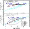 |
Fig. 9 Present-day oxygen abundance vs. M∗ as predicted by models with normal wind. All the models contain 7 bursts and the same burst sequence (ϵ = 0.2,n = 7,t = 1/3/5/7/9/11/13,d = 0.1 for each burst), and the total infall mass varies from Minf = 108 to 1010 M⊙. The upper panel shows results on a short infall timescale (τ = 1 Gyr), whereas the lower one shows results with a long timescale (τ = 10 Gyr). The predicted M − Z relation with different strengths of normal wind are shown by black lines: solid, dash-dotted, long-dashed, short-dashed, and dotted black lines are for λm = 0,0.2,0.5,1,3, respectively. Models with same Minf are connected by blue lines. An increasing wind efficiency to less massive galaxies is shown by a solid red line. Observational data are shown by open cyan circles (BCDs) and open cyan triangles (dIrrs), the solid cyan line is the best fit of all the data, as in Fig. 1. |
The metal-enhanced wind also has a dramatic influence on the μ − Z relation, as we show in the upper righthand panel of Fig. 10. The normal wind mainly reduces the gas fraction rather than the abundance, whereas the metal-enhanced wind is very powerful in reducing the metallicity of the galaxy.
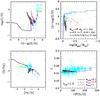 |
Fig. 10 The evolutionary track as predicted by models with various amounts of metal enhancements. The left two panels are log(C/O) vs. 12 + log(O/H) and [O/Fe] vs. [Fe/H]; the right two are oxygen abundance vs. gas fraction and Y vs. (O/H). All 3 models have the same burst sequence (t = 1/3/5/7/9/11/13 Gyr, and d = 0.1 Gyr for each burst), but different degrees of metal enhancement. The solid black lines, dashed red lines, dotted blue lines represent wH,He = 0.1,0.5,1, respectively. All these models assume the same total infall mass Minf = 109 M⊙. The observational data are the same as in Figs. 2–4, BCDs, dIrrs, and DLAs are plotted in open cyan circles, open cyan triangles, and open green squares here. |
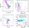 |
Fig. 11 The evolutionary track as predicted by models with various metal-enhanced wind efficiencies. The two left panels are log(C/O) vs. 12 + log(O/H) and [O/Fe] vs. [Fe/H]; the two right panels are oxygen abundance vs. gas fraction and Y vs. (O/H). All 5 models have the same burst sequence (t = 1/3/5/7/9/11/13 Gyr, and d = 0.1 Gyr for each burst), but different wind efficiencies. Solid green lines: λmw = 0; dash-dotted black lines: λmw = 0.2; long-dashed red lines: λmw = 1; short-dashed blue lines: λmw = 3; dotted magenta lines: λmw = 10. All these models assume the same total infall mass Minf = 109 M⊙. The observational data are the same as in Figs. 2–4, BCDs, dIrrs, and DLAs are plotted in open cyan circles, open cyan triangles, and open green squares here. |
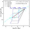 |
Fig. 12 Present-day oxygen abundance vs. M∗ as predicted by models with metal-enhanced wind (wH,He = 0.1). All the models contain 7 bursts and the same SFH (ϵ = 0.2,n = 7,t = 1/3/5/7/9/11/13,d = 0.1 for each burst), and the total infall mass varies from Minf = 108 to 1010 M⊙. The predicted M − Z relation with different strength of metal-enhanced wind are shown by different lines: dash-dotted, long-dashed, short-dashed, and dotted black lines are for λmw = 0,0.2,1,3 respective. Models with the same Minf are connected by blue lines. An increasing wind efficiency to less massive galaxies is shown by a solid red line, which can fit the data very well. Observational data are shown by open cyan circles (BCDs) and open cyan triangles (dIrrs), the solid cyan line is the best fit of all the data, as in Fig. 1. |
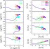 |
Fig. 13 The evolutionary track of abundance ratios of C/O, N/O, S/O, Si/O, C/Fe, N/Fe, O/Fe, and N/Si as predicted by our best models (Minf = 109 M⊙) with a metal-enhanced wind (wH,He = 0.3). The solid red, dash-dotted black, long-dashed magentaand short-dashed blue lines are the results for M9b1, M9b2, M9b3 and M9b4 in Table 3. The observational data are same as in Fig. 3, open cyan circles for BCDs and open green squares for DLAs. |
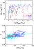 |
Fig. 14 The evolutionary tracks of 12+log(O/H) vs. gas fraction (upper panel) and Y − (O/H) relation (lower panel) as predicted by our best models (Minf = 109 M⊙) with metal-enhanced wind (wH,He = 0.3). The solid red, dash-dotted black, long-dashed magenta and short-dashed blue lines are the results of M9b1, M9b2, M9b3 and M9b4 in Table 3. The observational data are same as in Figs. 2 and 4, open cyan circles for BCDs and open cyan triangles for dIrrs. |
Models with different strengths (λmw = 0,0.2,1,3,10) of highly enriched winds (wH,He = 0.1) are shown in Fig. 11. We plot the evolutionary tracks of models with the same bursting history as in Fig. 10. A stronger wind not only reduces the abundances and increases the ratio between the long recycling term elements and the short ones, but it also decreases the gas fraction dramatically. It is worth pointing out that, although the wind efficiencies λmw adopted here are much higher than the ones of normal wind case λw, the gas is lost less effectively. To compare the results of normal and metal-enhanced wind models, one should assume a larger λmw for the latter case. For example, λmw = 10 for metal-enhanced winds is then multiplied by wH,He = 0.1, therefore it is comparable with the case normal wind and λw = 1.
In the lower righthand panels of both Figs. 10 and 11, we show the Y − (O/H) relations of galaxies with different degrees of enriched winds wH,He and different wind efficiencies λmw, but the same formation histories. By comparing with Fig. 8, the present-day oxygen abundances are lower, as expected. In this scenario, a very high helium abundance can be reached at a low metallicity level, especially when the wind is very strong, because most of it stays inside the galaxy while heavy elements are lost. The present-day Y − (O/H) relation predicted by these models do not stay on a straight line in the low-metallicity region, even if the unrealistic models (very strong wind λmw = 10 cases) are ruled out by their disagreement with other observational constraints. Therefore, the observed scatter of Y − (O/H) relation may be caused by metal-enhanced winds. Based on our model predictions, we suggest fitting the lower envelop of the observational data when one derives the primordial He Yp, because it may not be affected by the wind, so that the extrapolation to Z = 0 will be closer to the real Yp.
Figure 12 is the same as Fig. 9 but for models with metal-enhanced winds. Unlike the normal wind case, the metal-enhanced one is very effective in reducing the oxygen abundance, hence in creating the M − Z relation. The stronger the wind efficiency, the steeper the predicted M − Z. Therefore, models with an increasing wind efficiency to less massive galaxies are very consistent with the observations. As a conclusion, the observed M − Z relation could be caused by metal-enhanced winds with mild strengths (e.g., λmw ≤ 1).
In summary, metal-enhanced winds should take place in late-type dwarf galaxies, and they play an important role in removing gas, especially the metals, out of the galaxies.
4.4. Best models
As we have shown in the last section, highly enriched or very strong winds will reduce the galactic oxygen abundance to a very low value during the interburst time, which has not been confirmed from the observational point of view. Thus, in our best models wH,He = 0.3 and λmw = 0.8 are assumed. Different numbers of bursts are examined for Minf = 109 M⊙ galaxies, and the best-fit models are shown in Figs. 13 and 14. In these models, the same SFEs (ϵ = 0.5), and burst durations (d = 0.3) are assumed, and the details of each model are listed in Table 3.
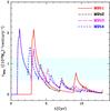 |
Fig. 15 The SN Ia rate normalized to the galaxy stellar mass as a function of time as predicted by our best models (Minf = 109 M⊙). The solid red, dash-dotted black, long-dashed magenta and short-dashed blue lines are for models M9b1, M9b2, M9b3, and M9b4, respectively. As a comparison, the shaded area shows the observed range of normalized SN Ia rate in the Irr galaxies, |
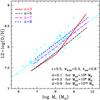 |
Fig. 16 The mass-metallicity relation as predicted by our best models. The total infalling masses range from Minf = 108 to 1010 M⊙, and the more massive one prefers a longer burst duration. The results with different numbers of burst are shown in different lines, solid red, dash-dotted black, long-dashed magenta, and short-dashed blue lines are for n = 3,5,7,9, respectively. The observational data of BCDs (open cyan circles) and dIrrs (open cyan triangles) are the same as in Fig. 1. |
We show the abundance ratios of different elements relative to oxygen or iron as predicted by our best models for Minf = 109 M⊙ in Fig. 13. The evolutionary tracks of these models can pass through the DLA data at an early time, and cover the regions where most of BCDs have been observed.
The evolutionary tracks of the μ − Z relation (upper panel) and Z − Y relation (lower panel) predicted by our best models are shown in Fig. 14. After the wind develops, the more bursts that a galaxy suffers, the more the oscillations in the evolutionary tracks, and these tracks pass through most of the data, thus explaining the observed spread. On the other hand, in the panel showing Y vs. (O/H) helium keeps increasing while O is oscillating, because this element is also produced during the interburst periods and lost less effectively than O. This implies again that we should use the lower envelop of the observational data to derive the primordial abundance of helium.
In Fig. 15, we show the evolution of the type Ia supernova rates predicted by our best models. The rates in this figure are normalized to the galaxy stellar mass at that time, i.e., expressed in number of SNe per century and per 1010 M⊙. The peaks are always associated with the SF periods, but SNe Ia also explode during the interburst times. Compared to the observed value quoted for the Irr galaxies,  per century and per 1010 M⊙ (Mannucci et al. 2005), our model predicts a very high normalized SN Ia rate during the first SF burst, but ~1–2 Gyr later, the rate decays and becomes comparable to the Irr galaxies in the following SF periods. In these best models, the maximum of SN Ia rate by number varies between 0.022 and 0.024 per century and the present value varies between 0.0012 and 0.0016 per century (see Table 4). Sullivan et al. (2006) have studied the relation between SN Ia rate and the stellar mass of the host galaxy in the redshift range 0.2–0.75, and they find the SN Ia rate is less than 0.01 per century for star-forming galaxies whose stellar mass around 108 M⊙, in agreement with our predictions.
To reproduce the mass-metallicity relation, we studied galaxies of different masses, with more massive galaxies preferring longer SF bursts, d = 0.9 Gyr for Minf = 1010 M⊙ and d = 0.1 Gyr for Minf = 108 M⊙ (see details in Table 3). The mass-metallicity relations predicted by our best models with different numbers of bursts are shown in Fig. 16, and they are consistent with the observed one considering the scatter of the data, especially in the cases where the wind develops in the whole galactic mass range (i.e., n ≥ 5).
Parameters of the best models (wH,He = 0.3).
Considering that dwarf galaxies could be in different evolutionary stages and/or have different ages (measured from the beginning of SF), we show that our best models – a series of uniform models with same Minf, wH, He, λmw, ϵ, d but different n and suitable t – can reproduce the spread in the observations well. Therefore, our preferred galaxy formation scenario for these galaxies is the following. They should have accreted a lot of primordial gas in their early stages, and formed stars through several short star bursts (d ~ 0.3 Gyr for Minf = 109 M⊙), with more massive galaxies suffering longer SF bursts. However, it is likely that the gas escapes from the potential well of the galaxy when enough energy from SN explosions is accumulated, and this wind should be metal-enhanced (wH, He ~ 0.3). The wind rate should be proportional to the gas mass at that time, and the wind efficiency should be λmw < 1.
DLAs could be the progenitors of dwarf irregular galaxies, as already suggested by Matteucci et al. (1997) and Calura et al. (2003). In our best models, we adopted a fixed duration for each burst with the purpose of changing the parameters as little as possible. The evolutionary tracks of our best models pass through the DLA data, but could not explain the scatter. However, if we reduce the duration of the first SF burst to d = 0.01 ~ 0.1 Gyr, by taking model M9b3 as an example, the models can explain the scatter in the abundance ratios of DLAs much better (see Fig. 17 and Table 3 for details of these models). Therefore, we confirm that the DLA systems could be progenitors of local dwarf galaxies.
4.5. Continuous star formation
By using a spectrophotometic model coupled with a chemical evolution model, Legrand (2000) demonstrats that a continuous but very mild SFR (SFE as low as 10-3 M⊙ Gyr-1) is able to reproduce the main properties of IZw 18, one of the most metal-poor BCDs we know. Therefore, in this section we show model results obtained with continuous and mild SF.
We ran the same models as in Legrand (2000), one model with only a mild continuous SF (ϵ = 0.001 Gyr-1), and the other with a mild continuous SF (ϵ = 0.001 Gyr-1) and a current burst (SFR = 0.023 M⊙ yr-1, i.e., ϵ = 0.88 Gyr-1 if the observed MHI = 2.6 × 10⁷ M⊙, during the past 20 Myr). The abundance ratios of different elements as predicted by these two models are shown in Fig. 18. As expected, such low continuous SF predicts too low a oxygen abundance, which could not explain the majority of local BCDs. In addition, by examining the evolutionary tracks in the low-metallicity range, one sees that DLAs cannot be the progenitors of such galaxies.
Therefore, we developed other models with higher SFEs and different SF duration. Since both dIrrs and BCDs harbor recent SF activities, we assumed that the SF is still going on today, and therefore a short duration d implies a late starting time (tG − d) of SF.
We examined the models with different SFHs by varying the SFE, duration, and infall timescale. The results show that only models with different SFEs are able to explain the scatters in the abundance ratios. In Fig. 19, models with different SFEs for the cases of no wind (left column), normal wind (middle column), and metal-enhanced wind (wH,He = 0.3, right column) are shown. In these models, to avoid reaching too high a metallicity at the present time, a duration shorter than the age of the universe is assumed for the highest SFE case. A short infall timescale is adopted (τ = 1 Gyr) here, because it does not affect the evolutionary track too much in the continuous SF scenario, especially when the SF starts late.
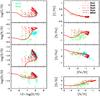 |
Fig. 17 The evolutionary track of abundance ratios as predicted by our DLA models. All of these models assume the same SFHs as model M9b3 except for a shorter duration for the first burst used. The red dotted, short-dash, long-dash and solid lines are for models DLA1 to DLA4 whose durations of the first burst are d = 0.01,0.02,0.05,0.1 Gyr, respectively. As a comparison, we also show the best model M9b2 of dwarf galaxy in dash-dotted black lines. All these models assume the same total infall mass Minf = 109 M⊙. Open cyan circles are BCDs and open green squares are DLAs, as in Fig. 3. |
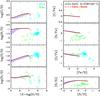 |
Fig. 18 The evolutionary track of abundance ratios as predicted by the models of Legrand (2000). A mild continuous SF with ϵ = 0.001 Gyr-1 is shown by solid black lines, whereas a mild continuous SF (ϵ = 0.001 Gyr-1) combined with a current burst (SFR = 0.023 M⊙ yr-1, i.e., ϵ = 0.88 Gyr-1 if MHI = 2.6 × 10⁷ M⊙, during the last 20 Myr) is shown in dashed red lines. The blue shade areas show the continuous SF with 1.45 × 10⁻³ ≤ ϵ ≤ 3.85 × 10⁻³ Gyr-1 which is derived from the observed SFR and MHI data of IZw 18 (see Table 1 of Legrand 2000). Cyan open circles are BCDs and open green squares are DLAs, as in Fig. 3. |
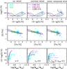 |
Fig. 19 The evolutionary track as predicted by models with continuous SF. From top to bottom, panels show log(C/O) vs. 12 + log(O/H), [O/Fe] vs. [Fe/H], and the μ − Z relation; from left to right columns are for the cases of no wind, normal wind, and metal-enhanced wind (wH, He = 0.3). Models with different SFEs are shown in each case: solid black lines for ϵ = 0.5 (d = 2), dash-dotted magenta lines for ϵ = 0.2 (d = 5), long-dashed blue lines for ϵ = 0.1 (d = 7), dashed red lines for ϵ = 0.05 (d = 9), and dotted black lines for ϵ = 0.02 (d = 13). The total infall masses are assumed to be Minf = 109 M⊙ in all these models. The observational data are the same as in Figs. 2 and 3, BCDs, dIrrs, and DLAs are plotted in open cyan circles, open cyan triangles, and open green squares, respectively. |
The maximum and present-day values of the SN Ia rates by number as predicted by the best models.
There are several conclusions that can be drawn from Fig. 19:
-
1.
in the case of no wind, although models with different ϵ could partly explain the scatters in the abundance ratios, they cannot reproduce the μ − Z relation. As we can see from the bottom lefthand panel of Fig. 19, all the evolutionary tracks overlap, the same as in the bursting SF scenario without galactic wind;
-
2.
when the wind is included in the model, the gas fraction decreases with time (the bottom middle and right panels of Fig. 19). We adopt relatively high wind efficiencies in the continuous SF scenario. When we compare the models with the same SFE in both normal wind and metal-enhanced wind cases, we can see that their gas fractions reach almost the same values at the present time since their gas loss rates are comparable (λw = wH,Heλmw = 0.6); however, their metals show different behaviors. The oxygen abundance decreases dramatically in the metal-enhanced wind case, thus explaining the scatter in μ − Z relation much better. In the meantime, the metal-enhanced wind model can fit the data relative to abundance ratios much more closely (upper and middle panels of right column in Fig. 19);
-
3.
as we have demonstrated above, galaxies with long, continuous, but mild SF (e.g., ϵ = 0.01, d = 13), which could be the case for some BCDs as suggested by the previous work (e.g., Legrand 2000; Legrand et al. 2000), should not be the majority owing to the predicted oxygen abundances that are too low. Their evolutionary tracks relative to abundance ratios also do not fit the data. In addition, DLAs cannot be the progenitors of these objects when abundance ratios are examined, because of the very high predicted values of N/O, N/Fe, and N/Si at low metallicity (see Fig. 18), at variance with the properties of DLAs;
-
4.
in the continuous SF scenario, the optimal models should have ϵ = 0.05–0.2, a duration of SF shorter than 13 Gyr, and metal-enhanced winds should occur, a situation similar to a long starburst scenario. Moreover, DLAs can be the progenitors of these galaxies.
5. Discussion and conclusions
We have discussed in detail the chemical evolution of late-type dwarf galaxies (dwarf irregular and blue compact galaxies) and used the most recent data as a comparison. We considered the measured abundances of single elements (He, C, N, O, S, Si, and Fe), as well as the gas masses. We assumed that the late-type dwarf galaxies form by cold gas accretion, and we ran models for different accreted baryonic masses (108,109, and 1010 M⊙). We tested both bursting and continuous SF. We then studied the development of galactic winds in detail by assuming a dark matter halo which is assumed ten times the amount of the baryonic mass and feedback from SNe and stellar winds. Our main conclusions follow.
-
1.
Galactic winds are needed to reproduce the main properties of late-type dwarf galaxies, and they should be metal-enhanced; that is to say, metals are usually carried away, in agreement with previous dynamical work (e.g. Mac Low & Ferrara 1999; Recchi et al. 2001). The rate of gas loss was assumed to be proportional to the amount of gas present at the time of the wind, which is equivalent to saying that is proportional to the SFR, in agreement with previous papers and observational evidence (Martin 2005; Rupke et al. 2005; Chen et al. 2010). The wind efficiency λmw should be relatively low (λmw ~ 0.8 in a bursting SF scenario, and λmw ~ 2 in a continuous SF scenario) compared to what is assumed for dwarf spheroidals (~6 to 15) where the wind should carry away all the residual gas (e.g. Lanfranchi & Matteucci 2003).
-
2.
Both bursting and continuous SF scenarios have been examined. In the case of bursting SF, the number of bursts could be no more than ~10 and the SFE could be ~0.5 Gyr-1. Galaxies with a long continuous, but mild SF (ϵ ≲ 0.02 Gyr-1, d ≃ 13 Gyr) should not be the majority, whereas galaxies with higher SFE (0.05 Gyr-1 ≲ ϵ ≲ 0.2 Gyr-1) and shorter SF duration (5 Gyr ≲ d ≲ 9 Gyr) are still acceptable.
-
3.
Models with a different number of bursts and/or different SFE and/or different burst duration, coupled with metal enhanced winds, can at best reproduce the spread observed in the abundances versus fractionary mass of gas and abundance ratios versus abundances. Normal winds, where all the gas and metals are lost at the same rate, should be rejected since they subtract too much gas.
-
4.
We studied the M − Z relation for late-type dwarf galaxies and showed that to reproduce such a relation one should assume that different galaxies suffered an increasing amount of SF (efficiency, number of bursts, duration of bursts) with galactic mass, even without galactic winds. However, metal-enhanced wind are needed to reproduce all the other features. In the case of the M − Z relation, a metal-enhanced wind efficiency increasing with galactic mass can reproduce the data very well, leaving all the other parameters to be the same irrespective of the galactic mass. On the other hand, normal winds occurring at different efficiencies in different galaxies cannot reproduce the M − Z relation unless the primordial gas is continuously infalling (i.e., on a long infall timescale) or the SFE or the number of bursts increases with galactic mass.
-
5.
A comparison of our best model predictions with data for DLAs has shown that these objects might well be the progenitors of local dIrrs and BCDs, in agreement with previous papers.
-
6.
Our models can reproduce the chemical properties of both dIrrs and BCDs. To distinguish between these two types of galaxies, the photometric and spectral information should also be taken into account.
Acknowledgments
J.Y. acknowledges the hospitality of the Department of Physics of the University of Trieste where this work was accomplished. J.Y. and F.M. acknowledge the financial support from PRIN2007 from Italian Ministry of Research, Prot. No. 2007JJC53X-001. J.Y. also acknowledges the financial support from the National Science Foundation of China Nos. 10573028 and 11143002, the Science Foundation of Shanghai No. 11ZR1443600, the Key Project No. 10833005, the Group Innovation Project No. 10821302, 973 program No. 2007CB815402, and the Knowledge Innovation Program of the Chinese Academy of Sciences No. Y090761009. Finally, we thank the referee, Leticia Carigi, for carefully reading the manuscript and giving us very useful suggestions.
References
- Abate, A., Bridle, S., Teodoro, L. F. A., Warren, M. S., & Hendry, M. 2008, MNRAS, 389, 1739 [NASA ADS] [CrossRef] [Google Scholar]
- Aloisi, A., Clementini, G., Tosi, M., et al. 2007, ApJ, 667, L151 [NASA ADS] [CrossRef] [Google Scholar]
- Bertin, G., Saglia, R. P., & Stiavelli, M. 1992, ApJ, 384, 423 [NASA ADS] [CrossRef] [Google Scholar]
- Bomans, D. J., Chu, Y.-H., & Hopp, U. 1997, ApJ, 113, 1678 [Google Scholar]
- Bradamante, F., Matteucci, F., & D’Ercole, A. 1998, A&A, 337, 338 [NASA ADS] [Google Scholar]
- Brodie, J. P., & Huchra, J. P. 1991, ApJ, 379, 157 [NASA ADS] [CrossRef] [Google Scholar]
- Calura, F., Matteucci, F., & Vladilo, G. 2003, MNRAS, 340, 59 [NASA ADS] [CrossRef] [Google Scholar]
- Carigi, L., Colín, P., & Peimbert, M. 1999, ApJ, 514, 787 [NASA ADS] [CrossRef] [Google Scholar]
- Centurión, M., Molaro, P., Vladilo, G., et al. 2003, A&A, 403, 55 [NASA ADS] [CrossRef] [EDP Sciences] [Google Scholar]
- Chen, Y. M., Tremonti, C. A., Heckman, T. M., et al. 2010, AJ, 140, 445 [NASA ADS] [CrossRef] [Google Scholar]
- Dekel, A., & Silk, J. 1986, ApJ, 303, 39 [NASA ADS] [CrossRef] [Google Scholar]
- Dessauges-Zavadsky, M., D’Odorico, S., McMahon, R. G., et al. 2001, A&A, 370, 426 [NASA ADS] [CrossRef] [EDP Sciences] [Google Scholar]
- Dessauges-Zavadsky, M., Calura, F., Prochaska, J. X., D’Odorico, S., & Matteucci, F. 2004, A&A, 416, 79 [NASA ADS] [CrossRef] [EDP Sciences] [Google Scholar]
- Dessauges-Zavadsky, M., Prochaska, J. X., D’Odorico, S., Calura, F., & Matteucci, F. 2006, A&A, 445, 93 [NASA ADS] [CrossRef] [EDP Sciences] [Google Scholar]
- Dessauges-Zavadsky, M., Calura, F., Prochaska, J. X., D’Odorico, S., & Matteucci, F. 2007, A&A, 470, 431 [NASA ADS] [CrossRef] [EDP Sciences] [Google Scholar]
- De Young, D. S., & Gallagher, J. S. 1990, ApJ, 356, 15 [Google Scholar]
- D’Odorico, V., & Molaro, P. 2004, A&A, 415, 879 [NASA ADS] [CrossRef] [EDP Sciences] [Google Scholar]
- Ekta, B., & Chengalur, J. N. 2010, MNRAS, 406, 1238 [NASA ADS] [Google Scholar]
- Ellison, S. L., & Lopez, S. 2001, A&A, 380, 117 [NASA ADS] [CrossRef] [EDP Sciences] [Google Scholar]
- Ellison, S. L., Pettini, M., Steidel, C. C., & Shapley, A. E. 2001, ApJ, 549, 770 [NASA ADS] [CrossRef] [Google Scholar]
- Fujita, A., Martin, C. L., Mac Low, M.-M., & Abel, T. 2003, ApJ, 599, 50 [NASA ADS] [CrossRef] [Google Scholar]
- Ferrara, A., & Tolstoy, E. 2000, MNRAS, 313, 291 [NASA ADS] [CrossRef] [Google Scholar]
- Garnett, D. R. 2002, ApJ, 581, 1019 [NASA ADS] [CrossRef] [MathSciNet] [Google Scholar]
- Garnett, D. R., & Shields, G. A. 1987, ApJ, 317, 82 [NASA ADS] [CrossRef] [Google Scholar]
- Grebel, E. K. 2001, ASPC, 239, 280 [NASA ADS] [Google Scholar]
- Guseva, N. G., Izotov, Y. I., Papaderos, P., et al. 2001, A&A, 378, 756 [NASA ADS] [CrossRef] [EDP Sciences] [Google Scholar]
- Guseva, N. G., Papaderos, P., Izotov, Y. I., et al. 2003a, A&A, 407, 91 [NASA ADS] [CrossRef] [EDP Sciences] [Google Scholar]
- Guseva, N. G., Papaderos, P., Izotov, Y. I., et al. 2003b, A&A, 407, 105 [NASA ADS] [CrossRef] [EDP Sciences] [Google Scholar]
- Henry, R. B. C., & Prochaska, J. X. 2007, PASP, 119, 962 [NASA ADS] [CrossRef] [Google Scholar]
- Henry, R. B. C., Edmunds, M. G., & Köppen, J. 2000, ApJ, 541, 660 [NASA ADS] [CrossRef] [Google Scholar]
- Izotov, Y. I., & Thuan, T. X. 1998a, ApJ, 497, 227 [NASA ADS] [CrossRef] [Google Scholar]
- Izotov, Y. I., & Thuan, T. X. 1998b, ApJ, 500, 188 [NASA ADS] [CrossRef] [Google Scholar]
- Izotov, Y. I., & Thuan, T. X. 1999, ApJ, 511, 639 [NASA ADS] [CrossRef] [Google Scholar]
- Izotov, Y. I., & Thuan, T. X. 2004a, ApJ, 602, 200 [CrossRef] [Google Scholar]
- Izotov, Y. I., & Thuan, T. X. 2004b, ApJ, 616, 768 [CrossRef] [Google Scholar]
- Izotov, Y. I., Thuan, T. X., & Lipovetsky, V. A. 1997, ApJS, 108, 1 [NASA ADS] [CrossRef] [Google Scholar]
- Izotov, Y. I., Chaffee, F. H., Foltz, C. B., et al. 1999, ApJ, 527, 757 [NASA ADS] [CrossRef] [Google Scholar]
- Izotov, Y. I., Chaffee, F. H., & Green, R. F. 2001a, ApJ, 562, 727 [NASA ADS] [CrossRef] [Google Scholar]
- Izotov, Y. I., Chaffee, F. H., & Schaerer, D. 2001b, A&A, 378, L45 [NASA ADS] [CrossRef] [EDP Sciences] [Google Scholar]
- Izotov, Y. I., Schaerer, D., Blecha, A., et al. 2006, A&A, 459, 71 [NASA ADS] [CrossRef] [EDP Sciences] [Google Scholar]
- Jenkins, E. B. 2009, ApJ, 700, 1299 [NASA ADS] [CrossRef] [Google Scholar]
- Karachentsev, I. D., Karachentseva, V. E., Huchtmeier, W. K., & Makarov, D. I. 2004, AJ, 127, 2031 [Google Scholar]
- Kauffmann, G., White, S. D. M., & Guiderdoni, B. 1993, MNRAS, 264, 201 [NASA ADS] [CrossRef] [Google Scholar]
- Kulkarni, V. P., Huang, K., Green, R. F., et al. 1996, MNRAS, 279, 197 [NASA ADS] [Google Scholar]
- Kunth, D., Maurogordato, S., & Vigroux, L. 1988, A&A, 204, 10 [NASA ADS] [Google Scholar]
- Lamareille, F., Mouhcine, M., Contini, T., Lewis, I., & Maddox, S. 2004, MNRAS, 350, 396 [NASA ADS] [CrossRef] [Google Scholar]
- Lanfranchi, G. A., & Matteucci, F. 2003, MNRAS, 345, 71 [NASA ADS] [CrossRef] [Google Scholar]
- Larson, R. 1974, MNRAS, 169, 229 [NASA ADS] [CrossRef] [Google Scholar]
- Lee, H., McCall, M. L., Kingsburgh, R., Ross, R., & Stevenson, C. C. 2003a, AJ, 125, 146 [NASA ADS] [CrossRef] [Google Scholar]
- Lee, H., McCall, M. L., & Richer, M. G. 2003b, AJ, 125, 2975 [NASA ADS] [CrossRef] [Google Scholar]
- Lee, J. C., Salzer, J. J., & Melbourne, J. 2004, ApJ, 616, 752 [NASA ADS] [CrossRef] [Google Scholar]
- Lee, H., Skillman, E. D., Cannon, J. M., et al. 2006, ApJ, 647, 970 [NASA ADS] [CrossRef] [Google Scholar]
- Ledoux, C., Petitjean, P., & Srianand, R. 2003, MNRAS, 346, 209 [NASA ADS] [CrossRef] [Google Scholar]
- Ledoux, C., Petitjean, P., Fynbo, J. P. U., Møller, P., & Srianand, R. 2006, A&A, 457, 71 [NASA ADS] [CrossRef] [EDP Sciences] [MathSciNet] [Google Scholar]
- Legrand, F. 2000, A&A, 354, 504 [NASA ADS] [Google Scholar]
- Legrand, F., Kunth, D., Roy, J.-R., Mas-Hesse, J. M., & Walsh, J. R. 2000, A&A, 355, 891 [NASA ADS] [Google Scholar]
- Lequeux, J., Peimbert, M., Rayo, J. F., Serrano, A., & Torres-Peimbert, S. 1979, A&A, 80, 155 [NASA ADS] [Google Scholar]
- Levshakov, S. A., Dessauges-Zavadsky, M., D’Odorico, S., & Molaro, P. 2002, ApJ, 565, 696 [NASA ADS] [CrossRef] [Google Scholar]
- Lipovetsky, V. A., Chaffee, F. H., Izotov, Y. I., et al. 1999, ApJ, 519, 177 [NASA ADS] [CrossRef] [Google Scholar]
- Lopez, S., & Ellison, S. L. 2003, A&A, 403, 573 [Google Scholar]
- Lopez, S., Reimers, D., D’Odorico, S., & Prochaska, J. X. 2002, A&A, 385, 778 [NASA ADS] [CrossRef] [EDP Sciences] [Google Scholar]
- Lu, L., Sargent, W. L. W., Barlow, T. A., Churchill, C. W., & Vogt, S. S. 1996, ApJS, 107, 475 [NASA ADS] [CrossRef] [Google Scholar]
- Luridiana, V., Peimbert, A., Peimbert, M., & Cerviño, M. 2003, ApJ, 592, 846 [NASA ADS] [CrossRef] [Google Scholar]
- Mac Low, M.-M., & Ferrara, A. 1999, ApJ, 513, 142 [NASA ADS] [CrossRef] [Google Scholar]
- Mannucci, F., Della valle, M., Panagia, N., et al. 2005, A&A, 433, 807 [NASA ADS] [CrossRef] [EDP Sciences] [Google Scholar]
- Marconi, G., Matteucci, F., & Tosi, M. 1994, MNRAS, 270, 35 [NASA ADS] [CrossRef] [Google Scholar]
- Martin, C. L. 1996, ApJ, 465, 680 [NASA ADS] [CrossRef] [Google Scholar]
- Martin, C. L. 2005, ApJ, 621, 227 [Google Scholar]
- Martin, C. L., Kobulnicky, H. A., & Heckman, T. M. 2002, ApJ, 574, 663 [NASA ADS] [CrossRef] [Google Scholar]
- Martín-Manjón, M. L., Mollá, M., Díaz, A. I., & Terlevich, R. 2008, MNRAS, 385, 854 [NASA ADS] [CrossRef] [Google Scholar]
- Martín-Manjón, M. L., Mollá, M., Díaz, A. I., & Terlevich, R. 2009 [arXiv:0901.1186] [Google Scholar]
- Mateo, M. 1998, ARA&A, 36, 435 [NASA ADS] [CrossRef] [Google Scholar]
- Matteucci, F., & Chiosi, C. 1983, A&A, 123, 121 [NASA ADS] [Google Scholar]
- Matteucci, F., & Tosi, M. 1985, MNRAS, 217, 391 [NASA ADS] [Google Scholar]
- Matteucci, F., Molaro, P., & Vladilo, G. 1997, A&A, 321, 45 [NASA ADS] [Google Scholar]
- Mendes de Oliveira, C., Temporin, S., Cypriano, E. S., et al. 2006, AJ, 132, 570 [NASA ADS] [CrossRef] [Google Scholar]
- Meurer, G. R., Freeman, K. C., Dopita, M. A., & Cacciari, C. 1992, AJ, 103, 60 [NASA ADS] [CrossRef] [Google Scholar]
- Molaro, P., Levshakov, S. A., D’Odorico, S., Bonifacio, P., & Centurión, M. 2001, ApJ, 549, 90 [NASA ADS] [CrossRef] [Google Scholar]
- Noterdaeme, P., Petitjean, P., Srianand, R., Ledoux, C., & Le Petit, F. 2007, A&A, 469, 425 [NASA ADS] [CrossRef] [EDP Sciences] [Google Scholar]
- Noterdaeme, P., Petitjean, P., Ledoux, C., Srianand, R., & Ivanchik, A. 2008, A&A, 491, 397 [NASA ADS] [CrossRef] [EDP Sciences] [Google Scholar]
- O’Meara, J. M., Burles, S., Prochaska, J. X., et al. 2006, ApJ, 649, L61 [NASA ADS] [CrossRef] [Google Scholar]
- Östlin, G. 2000, ApJ, 535, L99 [NASA ADS] [CrossRef] [PubMed] [Google Scholar]
- Outram, P. J., Chaffee, F. H., & Carswell, R. F. 1999, MNRAS, 310, 289 [NASA ADS] [CrossRef] [Google Scholar]
- Papaderos, P., Loose, H.-H., Thuan, T. X., & Fricke, K. J. 1996, A&AS, 120, 207 [NASA ADS] [CrossRef] [EDP Sciences] [Google Scholar]
- Papaderos, P., Izotov, Y. I., Thuan, T. X., et al. 2002, A&A, 393, 461 [NASA ADS] [CrossRef] [EDP Sciences] [Google Scholar]
- Papaderos, P., Guseva, N. G., Izotov, Y. I., et al. 2006, A&A, 457, 45 [NASA ADS] [CrossRef] [EDP Sciences] [Google Scholar]
- Peimbert, A. 2003, ApJ, 584, 735 [NASA ADS] [CrossRef] [Google Scholar]
- Peimbert, M., Luridiana, V., & Peimbert, A. 2007, ApJ, 666, 636 [NASA ADS] [CrossRef] [Google Scholar]
- Pérez-González, P. G., Gil de Paz, A., Zamorano, J., et al. 2003, MNRAS, 338, 525 [NASA ADS] [CrossRef] [Google Scholar]
- Péroux, C., Meiring, J. D., Kulkarni, V. P., et al. 2006, MNRAS, 372, 369 [NASA ADS] [CrossRef] [Google Scholar]
- Petitjean, P., Srianand, R., & Ledoux, C. 2000, A&A, 364, L26 [NASA ADS] [Google Scholar]
- Petitjean, P., Ledoux, C., & Srianand, R. 2008, A&A, 480, 349 [NASA ADS] [CrossRef] [EDP Sciences] [Google Scholar]
- Pettini, M., Ellison, S. L., Bergeron, J., & Petitjean, P. 2002, A&A, 391, 21 [NASA ADS] [CrossRef] [EDP Sciences] [MathSciNet] [Google Scholar]
- Pettini, M., Zych, B. J., Steidel, C. C., & Chaffee, F. H. 2008, MNRAS, 385, 2011 [NASA ADS] [CrossRef] [Google Scholar]
- Pilyugin, L. S. 1993, A&A, 277, 42 [NASA ADS] [Google Scholar]
- Pilyugin, L. S. 2001, A&A, 374, 412 [NASA ADS] [CrossRef] [EDP Sciences] [Google Scholar]
- Pilyugin, L. S., Vilchez, J. M., & Contini, T. 2004, A&A, 425, 849 [NASA ADS] [CrossRef] [EDP Sciences] [Google Scholar]
- Prochaska, J. X., Henry, R. B. C., O’Meara, J. M., et al. 2002a, PASP, 114, 933 [NASA ADS] [CrossRef] [Google Scholar]
- Prochaska, J. X., Howk, J. C., O’Meara, J. M., et al. 2002b, ApJ, 571, 693 [NASA ADS] [CrossRef] [Google Scholar]
- Prochaska, J. X., Gawiser, E., Wolfe, A. M., Cooke, J., & Gelino, D. 2003, ApJS, 147, 227 [NASA ADS] [CrossRef] [Google Scholar]
- Prochaska, J. X., Wolfe, A. M., Howk, J. C., et al. 2007, ApJS, 171, 29 [NASA ADS] [CrossRef] [Google Scholar]
- Prochaska, J. X., Chen, H., Wolfe, A. M., Dessauges-Zavadsky, M., & Bloom, J. S. 2008, ApJ, 672, 59 [NASA ADS] [CrossRef] [Google Scholar]
- Pustilnik, S. A., Pramskij, A. G., & Kniazev, A. Y. 2004, A&A, 425, 51 [NASA ADS] [CrossRef] [EDP Sciences] [Google Scholar]
- Recchi, S., Matteucci, F., & D’Ercole, A. 2001, MNRAS, 322, 800 [NASA ADS] [CrossRef] [Google Scholar]
- Recchi, S., Matteucci, F., & D’Ercole, A. 2002, A&A, 384, 799 [NASA ADS] [CrossRef] [EDP Sciences] [Google Scholar]
- Recchi, S., Matteucci, F., D’Ercole, A., & Tosi, M. 2004, A&A, 426, 37 [NASA ADS] [CrossRef] [EDP Sciences] [Google Scholar]
- Recchi, S., Spitoni, E., Matteucci, F., & Lanfranchi, G. A. 2008, A&A, 489, 555 [NASA ADS] [CrossRef] [EDP Sciences] [Google Scholar]
- Romano, D., Tosi, M., & Matteucci, F. 2006, MNRAS, 365, 759 [NASA ADS] [CrossRef] [MathSciNet] [Google Scholar]
- Rosenberg, J. L., Ashby, M. L. N., Salzer, J. J., & Huang, J.-S. 2006, ApJ, 636, 742 [NASA ADS] [CrossRef] [Google Scholar]
- Rupke, D. S., Veilleux, S., & Sanders, D. B. 2005, ApJS, 160, 115 [NASA ADS] [CrossRef] [Google Scholar]
- Salpeter, E. E., 1955, ApJ, 121, 161 [Google Scholar]
- Salzer, J. J., Lee, J. C., Melbourne, J., et al. 2005, ApJ, 624, 661 [NASA ADS] [CrossRef] [Google Scholar]
- Saviane, I., Ivanov, V. D., Held, E. V., et al. 2008, A&A, 487, 901 [NASA ADS] [CrossRef] [EDP Sciences] [Google Scholar]
- Scalo, J. M. 1986, Fund. Cosmic Phys., 11, 1 [NASA ADS] [EDP Sciences] [Google Scholar]
- Schmidt, M. 1963, ApJ, 137, 758 [NASA ADS] [CrossRef] [Google Scholar]
- Schulte-Ladbeck, R. E., Hopp, U., Greggio, L., Crone, M. M., & Drozdovsky, I. O. 2001, Ap&SS, 277, 309 [CrossRef] [Google Scholar]
- Searle, L., & Sargent, W. L. W. 1972, ApJ, 173, 25 [NASA ADS] [CrossRef] [Google Scholar]
- Searle, L., Sargent, W. L. W., & Bagnuolo, W. G. 1973, ApJ, 179, 427 [NASA ADS] [CrossRef] [Google Scholar]
- Skillman, E. D., Kennicutt, R. C., & Hodge, P. W. 1989, ApJ, 347, 875 [NASA ADS] [CrossRef] [Google Scholar]
- Skillman, E. D., Bomans, D. J., & Kobulnicky, H. A. 1997, ApJ, 474, 205 [NASA ADS] [CrossRef] [Google Scholar]
- Spergel, D. N., Bean, R., Doré, O., et al. 2007, ApJS, 170, 377 [NASA ADS] [CrossRef] [Google Scholar]
- Srianand, R., & Petitjean, P. 2001, A&A, 373, 816 [NASA ADS] [CrossRef] [EDP Sciences] [Google Scholar]
- Srianand, R., Petitjean, P., Ledoux, C., Ferland, G., & Shaw, G. 2005, MNRAS, 362, 549 [Google Scholar]
- Stasińska, G., & Izotov, Y. 2003, A&A, 397, 71 [NASA ADS] [CrossRef] [EDP Sciences] [Google Scholar]
- Staveley-Smith, L., Davies, R. D., & Kinman, T. D. 1992, MNRAS, 258, 334 [NASA ADS] [CrossRef] [Google Scholar]
- Storrie-Lombardi, L. J., & Wolfe, A. M. 2000, ApJ, 543, 552 [NASA ADS] [CrossRef] [Google Scholar]
- Sullivan, M., Borgne, D. Le, Pritchet, C. J., et al. 2006, ApJ, 648, 868 [NASA ADS] [CrossRef] [Google Scholar]
- Thuan, T. X. 2008, IAUS, 255, 348 [NASA ADS] [CrossRef] [Google Scholar]
- Thuan, T. X., Izotov, Y. I., & Lipovetsky, V. A. 1995, ApJ, 445, 108 [NASA ADS] [CrossRef] [Google Scholar]
- Thuan, T. X., Izotov, Y. I., & Foltz, C. B. 1999, ApJ, 525, 105 [NASA ADS] [CrossRef] [Google Scholar]
- Tosi, M., Greggio, L., Marconi, G., & Focardi, P. 1991, AJ, 102, 951 [NASA ADS] [CrossRef] [Google Scholar]
- Tremonti, C. A., Heckman, T. M., Kauffmann, G., et al. 2004, ApJ, 613, 898 [NASA ADS] [CrossRef] [Google Scholar]
- Vaduvescu, O., McCall, M. L., Richer, M. G., & Fingerhut, R. L. 2005, AJ, 130, 1593 [NASA ADS] [CrossRef] [Google Scholar]
- Vaduvescu, O., Richer, M. G., & McCall, M. L. 2006, AJ, 131, 1318 [NASA ADS] [CrossRef] [Google Scholar]
- Vaduvescu, O., McCall, M. L., & Richer, M. G., 2007, AJ, 134, 604 [NASA ADS] [CrossRef] [Google Scholar]
- van den Hoek, L. B., & Groenewegen, M. A. T. 1997, A&AS, 123, 305 [NASA ADS] [CrossRef] [EDP Sciences] [Google Scholar]
- van Zee, L., & Haynes, M. 2006, ApJ, 636, 214 [NASA ADS] [CrossRef] [Google Scholar]
- van Zee, L., Haynes, M. P., & Salzer, J. J. 1997, AJ, 114, 2497 [NASA ADS] [CrossRef] [Google Scholar]
- van Zee, L., Skillman, E. D., & Salzer, J. J. 1998, AJ, 116, 1186 [NASA ADS] [CrossRef] [Google Scholar]
- Vázquez, G. A., Carigi, L., & González, J. J. 2003, A&A, 400, 31 [NASA ADS] [CrossRef] [EDP Sciences] [Google Scholar]
- Vladilo, G. 2004, A&A, 421, 479 [NASA ADS] [CrossRef] [EDP Sciences] [Google Scholar]
- White, S. D. M., & Frenk, C. S. 1991, ApJ, 379, 52 [NASA ADS] [CrossRef] [Google Scholar]
- Woosley, S. E., & Weaver, T. A. 1995, ApJS, 101, 181 [NASA ADS] [CrossRef] [Google Scholar]
- Zaritsky, D., Kennicutt, R. C., Jr., & Huchra, J. P. 1994, ApJ, 420, 87 [NASA ADS] [CrossRef] [Google Scholar]
All Tables
The maximum and present-day values of the SN Ia rates by number as predicted by the best models.
All Figures
|
Fig. 1 Oxygen abundance vs. stellar mass for nearby dIrrs and BCDs. Filled blue and open magenta circles are data from Vaduvescu et al. (2007), and they represent BCDs and dIrrs, respectively; open magenta triangles are dIrrs observed by Lee et al. (2006), and the dashed line shows the best fit of their data. The solid line is the best linear fit of all the data. |
| In the text | |
|
Fig. 2 Oxygen abundance vs. gas fraction relation for nearby dIrrs and BCDs. Filled blue and open magenta circles are data from Vaduvescu et al. (2007), and they represent BCDs and dIrrs respectively; open magenta triangles are dIrrs observed by Lee et al. (2006); filled cyan triangles and squares are the Irrs observed by Pilyugin et al. (2004) and Garnett (2002), respectively. The solid line shows the prediction of the closed box model (Z = yZlnμ-1) with an effective yield yZ = 0.007 corresponding to the Salpeter IMF and Woosley & Weaver (1995) nucleosynthesis. |
| In the text | |
|
Fig. 3 Abundance ratio of different elements. Open blue circles are BCDs, from Izotov & Thuan (1999) and Papaderos et al. (2006); open green squares are DLAs, the data are shown in Table 1. |
| In the text | |
|
Fig. 4 Helium-metallicity (Y − Z) relation for Hii regions in BCDs, Fig. 2 of Izotov & Thuan (2004a). Filled green circles, from Izotov & Thuan (2004a); open red circles, from Izotov & Thuan (1998b); open blue triangles, from Izotov et al. (1997); open magenta pentagrams, from other data (Izotov & Thuan 1998a; Izotov et al. 1999; Thuan et al. 1999; Izotov et al. 2001a,b; Guseva et al. 2001, 2003a,b); the solid line is the maximum likelihood linear regression of all the data, Y = 0.2429 + 43 ∗ (O/H). |
| In the text | |
|
Fig. 5 The evolutionary tracks of [O/Fe] vs. [Fe/H] as predicted by models without outflow. a) Models with different number of bursts; b) models with different occurrence times of bursts; c) models with different durations of bursts; d) models with different SFE. All these models assume the same total infall mass Minf = 109 M⊙. The open cyan circles are BCDs and open green squares are DLAs, as in Fig. 3. |
| In the text | |
|
Fig. 6 Present oxygen abundance vs. gas fraction (upper panel) and Y vs. oxygen abundance (lower panel) as predicted by models without wind. All these models assume the same total infall mass Minf = 109 M⊙. Big open black circles: models with different numbers of bursts; big open black triangles: models with different durations of bursts; big open black squares: models with different occurrence times of bursts; big open black pentacles: models with different SFE. Solid black, dotted red and dashed blue lines in the upper panel are the evolutionary tracks of model M9d4, M9tau and M9IMF. The solid black line in the lower panel is the best fit of all the model points. The observational data are the same as in Figs. 2 and 4, open cyan circles and open cyan triangles represent BCDs and dIrrs, respectively. The solid cyan line is the best fit of the observational data. |
| In the text | |
|
Fig. 7 Present-day oxygen abundance vs. M∗ as predicted by models without wind. The upper (middle/lower) panel shows the model results with different numbers of bursts (durations/SFE), along the dashed blue lines the number of bursts (durations/SFE) increases from 2 to 7 (0.02 to 0.3/ 0.1 to 2), and along the solid black lines the total infall mass Minf increases from 108 to 1010 M⊙. The thick solid red line connects the models that are consistent with the observational data, larger n (d/ϵ) for more massive galaxy. The observational data are the same as in Fig. 1, open cyan circles for BCDs and open cyan triangles for dIrrs. |
| In the text | |
|
Fig. 8 The evolutionary track as predicted by models with normal wind. The left two panels are log(C/O) vs. 12 + log(O/H) and [O/Fe] vs. [Fe/H]; the right two panels are oxygen abundance vs. gas fraction and Y vs. (O/H). All the 5 models have the same bursts sequence (τ = 1 Gyr, t = 1/3/5/7/9/11/13 Gyr, and d = 0.1 Gyr for each burst), but different wind efficiencies, solid green lines for λm = 0, dash-dotted black lines for λm = 0.2, long-dashed red lines for λm = 0.5, and short-dashed blue lines for λm = 1. A model with long infall timescale (τ = 10 Gyr, λm = 1) is shown in magenta dotted line. All these models assume the same total infall mass Minf = 109 M⊙. The observational data are the same as in Figs. 2–4, BCDs, dIrrs, and DLAs are plotted in open cyan circles, open cyan triangles and open green squares here. |
| In the text | |
|
Fig. 9 Present-day oxygen abundance vs. M∗ as predicted by models with normal wind. All the models contain 7 bursts and the same burst sequence (ϵ = 0.2,n = 7,t = 1/3/5/7/9/11/13,d = 0.1 for each burst), and the total infall mass varies from Minf = 108 to 1010 M⊙. The upper panel shows results on a short infall timescale (τ = 1 Gyr), whereas the lower one shows results with a long timescale (τ = 10 Gyr). The predicted M − Z relation with different strengths of normal wind are shown by black lines: solid, dash-dotted, long-dashed, short-dashed, and dotted black lines are for λm = 0,0.2,0.5,1,3, respectively. Models with same Minf are connected by blue lines. An increasing wind efficiency to less massive galaxies is shown by a solid red line. Observational data are shown by open cyan circles (BCDs) and open cyan triangles (dIrrs), the solid cyan line is the best fit of all the data, as in Fig. 1. |
| In the text | |
|
Fig. 10 The evolutionary track as predicted by models with various amounts of metal enhancements. The left two panels are log(C/O) vs. 12 + log(O/H) and [O/Fe] vs. [Fe/H]; the right two are oxygen abundance vs. gas fraction and Y vs. (O/H). All 3 models have the same burst sequence (t = 1/3/5/7/9/11/13 Gyr, and d = 0.1 Gyr for each burst), but different degrees of metal enhancement. The solid black lines, dashed red lines, dotted blue lines represent wH,He = 0.1,0.5,1, respectively. All these models assume the same total infall mass Minf = 109 M⊙. The observational data are the same as in Figs. 2–4, BCDs, dIrrs, and DLAs are plotted in open cyan circles, open cyan triangles, and open green squares here. |
| In the text | |
|
Fig. 11 The evolutionary track as predicted by models with various metal-enhanced wind efficiencies. The two left panels are log(C/O) vs. 12 + log(O/H) and [O/Fe] vs. [Fe/H]; the two right panels are oxygen abundance vs. gas fraction and Y vs. (O/H). All 5 models have the same burst sequence (t = 1/3/5/7/9/11/13 Gyr, and d = 0.1 Gyr for each burst), but different wind efficiencies. Solid green lines: λmw = 0; dash-dotted black lines: λmw = 0.2; long-dashed red lines: λmw = 1; short-dashed blue lines: λmw = 3; dotted magenta lines: λmw = 10. All these models assume the same total infall mass Minf = 109 M⊙. The observational data are the same as in Figs. 2–4, BCDs, dIrrs, and DLAs are plotted in open cyan circles, open cyan triangles, and open green squares here. |
| In the text | |
|
Fig. 12 Present-day oxygen abundance vs. M∗ as predicted by models with metal-enhanced wind (wH,He = 0.1). All the models contain 7 bursts and the same SFH (ϵ = 0.2,n = 7,t = 1/3/5/7/9/11/13,d = 0.1 for each burst), and the total infall mass varies from Minf = 108 to 1010 M⊙. The predicted M − Z relation with different strength of metal-enhanced wind are shown by different lines: dash-dotted, long-dashed, short-dashed, and dotted black lines are for λmw = 0,0.2,1,3 respective. Models with the same Minf are connected by blue lines. An increasing wind efficiency to less massive galaxies is shown by a solid red line, which can fit the data very well. Observational data are shown by open cyan circles (BCDs) and open cyan triangles (dIrrs), the solid cyan line is the best fit of all the data, as in Fig. 1. |
| In the text | |
|
Fig. 13 The evolutionary track of abundance ratios of C/O, N/O, S/O, Si/O, C/Fe, N/Fe, O/Fe, and N/Si as predicted by our best models (Minf = 109 M⊙) with a metal-enhanced wind (wH,He = 0.3). The solid red, dash-dotted black, long-dashed magentaand short-dashed blue lines are the results for M9b1, M9b2, M9b3 and M9b4 in Table 3. The observational data are same as in Fig. 3, open cyan circles for BCDs and open green squares for DLAs. |
| In the text | |
|
Fig. 14 The evolutionary tracks of 12+log(O/H) vs. gas fraction (upper panel) and Y − (O/H) relation (lower panel) as predicted by our best models (Minf = 109 M⊙) with metal-enhanced wind (wH,He = 0.3). The solid red, dash-dotted black, long-dashed magenta and short-dashed blue lines are the results of M9b1, M9b2, M9b3 and M9b4 in Table 3. The observational data are same as in Figs. 2 and 4, open cyan circles for BCDs and open cyan triangles for dIrrs. |
| In the text | |
|
Fig. 15 The SN Ia rate normalized to the galaxy stellar mass as a function of time as predicted by our best models (Minf = 109 M⊙). The solid red, dash-dotted black, long-dashed magenta and short-dashed blue lines are for models M9b1, M9b2, M9b3, and M9b4, respectively. As a comparison, the shaded area shows the observed range of normalized SN Ia rate in the Irr galaxies, |
| In the text | |
|
Fig. 16 The mass-metallicity relation as predicted by our best models. The total infalling masses range from Minf = 108 to 1010 M⊙, and the more massive one prefers a longer burst duration. The results with different numbers of burst are shown in different lines, solid red, dash-dotted black, long-dashed magenta, and short-dashed blue lines are for n = 3,5,7,9, respectively. The observational data of BCDs (open cyan circles) and dIrrs (open cyan triangles) are the same as in Fig. 1. |
| In the text | |
|
Fig. 17 The evolutionary track of abundance ratios as predicted by our DLA models. All of these models assume the same SFHs as model M9b3 except for a shorter duration for the first burst used. The red dotted, short-dash, long-dash and solid lines are for models DLA1 to DLA4 whose durations of the first burst are d = 0.01,0.02,0.05,0.1 Gyr, respectively. As a comparison, we also show the best model M9b2 of dwarf galaxy in dash-dotted black lines. All these models assume the same total infall mass Minf = 109 M⊙. Open cyan circles are BCDs and open green squares are DLAs, as in Fig. 3. |
| In the text | |
|
Fig. 18 The evolutionary track of abundance ratios as predicted by the models of Legrand (2000). A mild continuous SF with ϵ = 0.001 Gyr-1 is shown by solid black lines, whereas a mild continuous SF (ϵ = 0.001 Gyr-1) combined with a current burst (SFR = 0.023 M⊙ yr-1, i.e., ϵ = 0.88 Gyr-1 if MHI = 2.6 × 10⁷ M⊙, during the last 20 Myr) is shown in dashed red lines. The blue shade areas show the continuous SF with 1.45 × 10⁻³ ≤ ϵ ≤ 3.85 × 10⁻³ Gyr-1 which is derived from the observed SFR and MHI data of IZw 18 (see Table 1 of Legrand 2000). Cyan open circles are BCDs and open green squares are DLAs, as in Fig. 3. |
| In the text | |
|
Fig. 19 The evolutionary track as predicted by models with continuous SF. From top to bottom, panels show log(C/O) vs. 12 + log(O/H), [O/Fe] vs. [Fe/H], and the μ − Z relation; from left to right columns are for the cases of no wind, normal wind, and metal-enhanced wind (wH, He = 0.3). Models with different SFEs are shown in each case: solid black lines for ϵ = 0.5 (d = 2), dash-dotted magenta lines for ϵ = 0.2 (d = 5), long-dashed blue lines for ϵ = 0.1 (d = 7), dashed red lines for ϵ = 0.05 (d = 9), and dotted black lines for ϵ = 0.02 (d = 13). The total infall masses are assumed to be Minf = 109 M⊙ in all these models. The observational data are the same as in Figs. 2 and 3, BCDs, dIrrs, and DLAs are plotted in open cyan circles, open cyan triangles, and open green squares, respectively. |
| In the text | |
Current usage metrics show cumulative count of Article Views (full-text article views including HTML views, PDF and ePub downloads, according to the available data) and Abstracts Views on Vision4Press platform.
Data correspond to usage on the plateform after 2015. The current usage metrics is available 48-96 hours after online publication and is updated daily on week days.
Initial download of the metrics may take a while.