| Issue |
A&A
Volume 694, February 2025
|
|
|---|---|---|
| Article Number | A147 | |
| Number of page(s) | 29 | |
| Section | Planets, planetary systems, and small bodies | |
| DOI | https://doi.org/10.1051/0004-6361/202452152 | |
| Published online | 07 February 2025 | |
MINDS
The influence of outer dust disc structure on the volatile delivery to the inner disc
1
Institute of Astronomy,
Celestijnenlaan 200D,
3001
Leuven,
Belgium
2
Leiden Observatory, Leiden University,
2300 RA
Leiden,
The Netherlands
3
Max-Planck Institut für Extraterrestrische Physik (MPE),
Giessen-bachstr. 1,
85748
Garching,
Germany
4
Université Paris-Saclay, CNRS, Institut d’Astrophysique Spatiale,
91405
Orsay,
France
5
Max-Planck-Institut für Astronomie (MPIA),
Königstuhl 17,
69117
Heidelberg,
Germany
6
Kapteyn Astronomical Institute, Rijksuniversiteit Groningen,
Postbus 800,
9700AV
Groningen,
The Netherlands
7
Dept. of Astrophysics, University of Vienna,
Türkenschanzstr. 17,
1180
Vienna,
Austria
8
ETH Zürich, Institute for Particle Physics and Astrophysics,
Wolfgang-Pauli-Str. 27,
8093
Zürich,
Switzerland
9
Centro de Astrobiología (CAB), CSIC-INTA, ESAC Campus,
Camino Bajo del Castillo s/n,
28692
Villanueva de la Cañada, Madrid,
Spain
10
INAF -– Osservatorio Astronomico di Capodimonte,
Salita Moiariello 16,
80131
Napoli,
Italy
11
Dublin Institute for Advanced Studies,
31 Fitzwilliam Place,
D02 XF86
Dublin,
Ireland
12
Department of Astrophysics/IMAPP, Radboud University,
PO Box 9010,
6500 GL
Nijmegen,
The Netherlands
13
SRON Netherlands Institute for Space Research,
Niels Bohrweg 4,
2333 CA
Leiden,
The Netherlands
14
Space Research Institute, Austrian Academy of Sciences,
Schmiedlstr. 6,
A-8042,
Graz,
Austria
15
TU Graz, Fakultät für Mathematik, Physik und Geodäsie,
Petersgasse 16,
8010
Graz,
Austria
16
Niels Bohr Institute, University of Copenhagen,
NBB BA2, Jagtvej 155A,
2200
Copenhagen,
Denmark
★ Corresponding author; This email address is being protected from spambots. You need JavaScript enabled to view it.
Received:
6
September
2024
Accepted:
20
December
2024
Abstract
Context. The Atacama Large Millimeter/submillimeter Array (ALMA) has revealed that the millimetre dust structures of protoplanetary discs are extremely diverse, ranging from small and compact dust discs to large discs with multiple rings and gaps. It has been proposed that the strength of H2O emission in the inner disc particularly depends on the influx of icy pebbles from the outer disc, a process that would correlate with the outer dust disc radius, and that could be prevented by pressure bumps. Additionally, the dust disc structure should also influence the emission of other gas species in the inner disc. Since terrestrial planets likely form in the inner disc regions, understanding their composition is of interest.
Aims. This work aims to assess the influence of pressure bumps on the inner disc’s molecular reservoirs. The presence of a dust gap, and potentially giant planet formation farther out in the disc, may influence the composition of the inner disc, and thus the building blocks of terrestrial planets.
Methods. Using the improved sensitivity and spectral resolution of the Mid-InfraRed Instrument’s (MIRI) Medium Resolution Spectrometer (MRS) on the James Webb Space Telescope (JWST) compared to Spitzer, we compared the observational emission properties of H2O, HCN, C2H2, and CO2 with the outer dust disc structure from ALMA observations, in eight discs with confirmed gaps in ALMA observations, and two discs with gaps of tens of astronomical units in width, around stars with M⋆ ≥ 0.45 M⊙ . We used new visibility plane fits of the ALMA data to determine the outer dust disc radius and identify substructures in the discs.
Results. We find that the presence of a dust gap does not necessarily result in weak H2O emission. Furthermore, the relative lack of colder H2O-emission seems to go hand in hand with elevated emission from carbon-bearing species. Of the discs that show significant substructure within the CO and CH4 snowlines, most show detectable emission from the carbon-bearing species. The discs with cavities and extremely wide gaps appear to behave as a somewhat separate group, with stronger cold H2O emission and weak warm H2O emission.
Conclusions. We conclude that fully blocking radial dust drift from the outer disc seems difficult to achieve, even for discs with very wide gaps or cavities, which can still show significant cold H2O emission. However, there does seem to be a dichotomy between discs that show a strong cold H2O excess and ones that show strong emission from HCN and C2H2. Better constraints on the influence of the outer dust disc structure and inner disc composition require more information on substructure formation timescales and disc ages, along with the importance of trapping of (hyper)volatiles like CO and CO2 into more strongly bound ices like H2O and chemical transformation of CO into less volatile species.
Key words: astrochemistry / protoplanetary disks / stars: variables: T Tauri, Herbig Ae/Be / infrared: planetary systems / submillimeter: planetary systems
© The Authors 2025
 Open Access article, published by EDP Sciences, under the terms of the Creative Commons Attribution License (https://creativecommons.org/licenses/by/4.0), which permits unrestricted use, distribution, and reproduction in any medium, provided the original work is properly cited.
This article is published in open access under the Subscribe to Open model. This email address is being protected from spambots. You need JavaScript enabled to view it. to support open access publication.
1 Introduction
The inner 10 au of protoplanetary discs observable with the Medium Resolution Spectrometer (MRS; Wells et al. 2015; Argyriou et al. 2023) of the Mid-InfraRed Instrument (MIRI; Wright et al. 2015; Rieke et al. 2015; Wright et al. 2023) on board the James Webb Space Telescope (JWST ; Rigby et al. 2023) is known to host active chemistry due to high temperatures and densities. This part of discs is of particular interest, as it is likely where terrestrial planets form (e.g. Öberg & Bergin 2021; Mollière et al. 2022). This region has been studied previously with Spitzer’s InfraRed Spectrograph (IRS) (e.g. Pascucci et al. 2009; Pontoppidan et al. 2010; Carr & Najita 2011; Pascucci et al. 2013; Pontoppidan et al. 2014), and ground-based data (e.g. Brown et al. 2013; Banzatti et al. 2022, 2023b), but the launch of JWST allows us to re-evaluate these regions with an improved sensitivity and spectral resolution (e.g. Kóspál et al. 2023; Grant et al. 2023; Tabone et al. 2023; Schwarz et al. 2024; Arabhavi et al. 2024). Importantly, H2O emission can be studied in more detail (e.g. Gasman et al. 2023b; Banzatti et al. 2023a; Pontoppidan et al. 2024; Temmink et al. 2024a; Romero-Mirza et al. 2024), with the first detection of H2O in a disc with confirmed planets by Perotti et al. (2023). The link between inner disc composition and the composition of the planets formed there is still a topic of debate (see Öberg & Bergin 2021, for a review); therefore understanding the mechanisms that influence the species available for accretion onto protoplanets in the inner disc is of interest. However, the emission from different discs observed with JWST has proven to be diverse, ranging from H2O-rich discs and strong silicate features to carbon-dominated discs and weak silicate features (Kamp et al. 2023; van Dishoeck et al. 2023; Henning et al. 2024).
Observations of protoplanetary discs using the Atacama Large Millimeter/submillimeter Array (ALMA) demonstrate an equally large variety in outer dust disc structure (e.g. Huang et al. 2018; Long et al. 2018, 2019). Some dust discs are very compact (e.g. Ansdell et al. 2016; Long et al. 2019), while others are extremely large and contain rings and gaps (e.g. V1094 Sco and Sz 98 in van Terwisga et al. 2018), and some even show spiral structures (e.g. IM Lup in Andrews et al. 2018). In this work, we make the distinction between gaps and cavities, whereby cavities span from the star to the start of the dust disc, while gaps are annular substructures located within the disc. An extensive list of mechanisms exists that can explain the formation of pressure bumps and other substructures (see Bae et al. 2023, for an overview), one of which is planet formation. We note, however, that the structures within the dust do not have to coincide with that of the gas (Öberg et al. 2021), or have the same depth, such as for CO and its isotopologues, which are generally less deep (van der Marel et al. 2016).
In the days of Spitzer, a range of sample studies pointed to a variety of correlations between the outer dust disc structure and molecular emission from the inner 0.1–10 au of the disc, mainly with H2O gas emission. For example, Carr & Najita (2011) and Najita et al. (2013) examined the ratio of HCN to H2O as a volatile C/O tracer, and found it to increase with increasing disc mass. They attribute this to sequestration of H2O-ice in the outer disc due to planetesimal formation, which would be more efficient for more massive discs. Similarly, Banzatti et al. (2020) find H2O line fluxes to be stronger for smaller dust disc sizes, which is a potential tracer for efficient pebble drift delivering H2O to the inner disc. In these works and the work presented here, we differentiate between the larger dust pebbles that move decoupled from the gas, and smaller micron-sized dust grains. Recently, Banzatti et al. (2023a) put this to the test using four T Tauri discs observed with MIRI/MRS. Their sample, consisting of two extended dust discs (IQ Tau and CI Tau) and two compact discs (GK Tau and HP Tau), seems to follow this anti-correlation between H2O line flux and dust disc size. Additionally, they find a cold reservoir of H2O (near sublimation temperatures; 170–400 K) in the smaller discs, indicative of pebble drift. They posit, based on for example Meijerink et al. (2009); Krijt et al. (2018), that without pebble drift the colder regions in the disc would quickly be depleted of H2O-gas due to the cold-finger effect trapping H2O in the form of ice. Drift would replenish this reservoir and produce a cold excess due to sublimation and diffusion at the snowline. One additional important factor is gap formation (Banzatti et al. 2017). Pebble drift can be prevented by substructures like gaps and rings in the outer disc. Sufficiently deep gaps can trap icy pebbles outside the H2O snowline, resulting in weak H2O emission and a lack of a cold reservoir. All of this indicates that there is observational evidence for the influence of the dust disc structure, like that derived from ALMA, on the ice species that reach the inner disc, and by extension its chemical composition, as has previously been seen with Spitzer, and now MIRI/MRS.
From a theoretical point of view, some modelling efforts exist that aim to link the evolution of the dust disc structure to the abundances of gas species in the inner disc. For example, Booth et al. (2017) and Booth & Ilee (2019) find that when transport of dust is sufficiently rapid, the abundance of gas species are enhanced within their respective snowlines due to sublimation from incoming ices. Initially, due to the sequence in H2O, CO2, and CO snowlines from closer to farther away from the star, the gaseous C/O and C/H ratios in the inner disc become sub- and super-solar, respectively. Over time, the H2O-gas will be accreted onto the star first, after which CO2 and CO are accreted, resulting in a more carbon-dominated inner disc as the disc evolves further (see also Mah et al. 2023).
Vlasblom et al. (2024) model the influence of a cavity on the H2O and CO2 content within the disc. They show that if the cavity extends past the H2O snowline, H2O emission will be suppressed, and the resulting spectrum is dominant in CO2 instead. This variation in inner disc emission with cavity size was also observed by Woitke et al. (2018).
Alternatively, Kalyaan et al. (2021, 2023) examine the influence of pebble drift in more detail for H2O, with the presence of gaps within the disc included, rather than a cavity. They find that the gaseous enhancement, at least for H2O, is temporary, lasting until the H2O gas has been accreted onto the central star. This means that the phase for which H2O is actually enhanced is relatively short-lived (up to a few million years or less), although this might be extended significantly if the gap only partially blocks the influx of dust pebbles (Mah et al. 2024) or even smaller dust grains (Pinilla et al. 2024). According to Sellek et al. (2025), this enhancement may not be directly visible in column densities derived from MRS spectra, due to an increased dust opacity as a result of drifting dust. They find the column density ratio between CO2 / H2O to be a more reliable drift tracer. Furthermore, both Kalyaan et al. (2023) and Sellek et al. (2025) note that the radial location of the gap is of influence: gaps closer to the star are more effective at reducing the H2O-gas enhancement, since more dust is located outside the gap, while a gap too far from the star blocks only a small part of the H2O-ice reservoir and is less effective. However, in some of the aforementioned models (Booth et al. 2017; Booth & Ilee 2019; Mah et al. 2024; Sellek et al. 2025) gas can move inwards over time, and even diffuse across gaps. This is in line with the expectations of gaps carved by planet formation, which are likely not efficient at blocking gas and the gaps can be leaky to small dust grains (Lubow & D’Angelo 2006; Bergez-Casalou et al. 2020; Kalyaan et al. 2021, 2023; Sellek et al. 2025). On the other hand, Lienert et al. (2024) also model gaps formed due to photoevaporation by X-rays, which could prevent all transport across the gap, even by gas. While the gap itself continues to only block dust transport, the photoevaporative winds blow gas away from the gap (e.g. Alexander et al. 2014; Pascucci et al. 2023).
Since the modelling efforts demonstrate that the enhancement can be variable in time, whether or not the increase in H2O-line flux becomes visible then depends on when gaps are formed and at what stage in the lifetime of the disc it is observed. Even relatively young discs, such as the young Class II object HL Tau (ALMA Partnership 2015) and Class I object IRS 63 (Segura-Cox et al. 2020), can have observable, albeit weak, substructures meaning that diversity in inner disc compositions due to the outer disc structure can already start early in the lifetimes of discs. However, the Class I objects being studied in the eDisks ALMA large programme (Ohashi et al. 2023) show no deep, detectable substructure, indicating that their formation likely occurs on the cusp of the transition between the Class I and Class II phases. Early substructure formation is supported by recent population synthesis modelling work (Delussu et al. 2024). We do note that disc and stellar age estimations often still have large uncertainties (e.g. Miotello et al. 2023).
Contrary to the above, Sz 98 is an example of a large dust disc (~180 au) with multiple gaps, but is found to be more dominant in H2O than carbon-bearing species (Gasman et al. 2023b), indicating that the story is more complex. Furthermore, drifting dust pebbles will not only contain H2O-ice; other ices should also be drifting inwards along with the dust, and could show some enhancement akin to the findings of Booth & Ilee (2019). Due to the sequence in H2O, CO2, and CO snowlines and theorised influence of dust drift on the inner disc composition, it naturally follows that both the presence and radial location of gaps may not only influence the presence of H2O in the inner disc, but also that of other oxygen- and carbon-bearing species. However, this relies on ices being released into the gas at their respective snowlines. This notion of sequential snowlines has been pointed out to not be entirely realistic. Lab works show that other volatiles can be trapped in H2O ice (e.g. Collings et al. 2004), and H2O ice in turn can be trapped within refractories, such as silicates (Potapov et al. 2024). As a result, the gaseous volatile ratios become much less dependent on the radial location in the disc, and instead several snowlines exist per species depending on the layering within the ice. For example, many volatiles are released along with H2O at the H2O snowline (e.g. Viti et al. 2004; Visser et al. 2009; Ligterink et al. 2024), and active chemistry occurs in the cold outer disc (Eistrup et al. 2018). This can transform CO into less volatile species, such as CH3OH and CO2 (e.g. Yu et al. 2016; Bosman et al. 2018).
Furthermore, radial transport of dust is not the only possible explanation for differences in emitting strength of species between discs. An increase in emission strength from all species can also be achieved by (1) increasing the ratio between the gas and dust, or (2) more transparent dust due to grain growth or dust settling, where both scenarios result in emission from a larger column of gas (e.g. Meijerink et al. 2009; Antonellini et al. 2015; Woitke et al. 2018). However, due to the variation in where the majority of different gas species are located spatially, changes in the dust opacity can influence the emission of certain molecules more strongly than others. For example, the relative strength of HCN compared to H2O increases with a decrease in dust opacity (Antonellini et al. 2023).
In this work, we explore the variation between the MIRI/MRS spectra of a sample of discs, most of which are part of the MIRI mid-INfrared Disk Survey (MINDS, Henning et al. 2024; Kamp et al. 2023). In order to test whether the presence of a gap close to the star reduces the flux of H2O and increases that of carbon-bearing species in the inner disc, we compare the emission from commonly detected species H2O, HCN, C2H2, and CO2 to the dust disc structure as found in ALMA data. To this end, we reanalyse ALMA continuum data to find the outer dust disc structures in a consistent manner.
The work presented here is structured as follows. First, the sample used, data reduction method, and lines used in this study are described in Sect. 2. The molecular emission in the sample is presented in Sect. 3. We compare these to the dust disc structure and put these in context of disc chemistry and planet formation in Sect. 4. The summary of the findings can be found in Sect. 5.
2 Methods
2.1 Sample
The sample presented here is a selection of discs around T Tauri stars, from two JWST programmes. The majority of the sources come from the MINDS programme, which is one of the Guaranteed Time Observation programmes of JWST (PID: 1282, PI: T. Henning). The total sample consists of 52 targets, out of which 33 are discs around T Tauri stars (Kamp et al. 2023; Henning et al. 2024). The second is PID 1640 (PI: A. Banzatti), which consists of eight different targets. Out of these 41 T Tauri discs, we excluded discs known to be in binary systems, discs with confirmed spiral features in millimetre emission, and highly inclined discs (i > 70°). Furthermore, it has already been demonstrated that discs of very low-mass objects show significantly different emission features, perhaps due to a difference in evolution timescale as compared to objects of higher mass (e.g. Mah et al. 2023), resulting in extremely hydrocarbon-rich discs (e.g. Tabone et al. 2023; Arabhavi et al. 2024; Kanwar et al. 2024, Morales-Caleron, in prep.). For gap formation to then influence the composition of the inner disc, gaps must form even earlier in the disc’s lifetime. Furthermore, due to the lower temperatures in these discs, gaps must be located much closer to the central star in order to still block oxygen-rich ices. To ensure our sample is homogeneous, the objects are selected to have at least M★ ≥ 0.45 M⊙.
Since our aim is to study the influence of gaps, only discs with confirmed gaps in millimetre dust are included, based on previously published results (Clarke et al. 2018; van Terwisga et al. 2018; Rosotti et al. 2021; Jennings et al. 2022a,b; Zhang et al. 2023). After carefully selecting the sample based on the aforementioned criteria, eight full discs from the two programmes remain and are listed in Table 1. Six of these are from the MINDS programme, along with two discs out of the eight targets from PID 1640, for which the H2O data are presented in Banzatti et al. (2023a). We further compare these cases to discs with extremely wide gaps of several tens of astronomical units, where transport may be most limited: two discs from MINDS (PID 1282), PDS 70 and SY Cha. Despite the large gaps, both PDS 70 and SY Cha have H2O emission in the inner disc (Perotti et al. 2023; Schwarz et al. 2024), and signs for transport across their large gaps (Orihara et al. 2023; Jang et al. 2024). For these reasons, they are interesting additions to the sample presented here. The associated PID and date of observation per target and other properties are summarised in Table 1.
2.2 Data reduction
For consistency, all data were reduced using version 1.15.1 of the standard JWST pipeline (Bushouse et al. 2023), and pmap 1252. While targets observed at the start of the MINDS programme make use of target acquisition, a large part of the sample taken later in the year did not. As such, the data cannot consistently be processed based on the methods presented by Gasman et al. (2023a) as was done in Grant et al. (2023) and Gasman et al. (2023b), or using asteroids as in Banzatti et al. (2023a) and Pontoppidan et al. (2024). To ensure that differences in the data reduction methods do not affect the relative fluxes between targets, we used the standard pipeline set-up, with extended fringe flats and residual fringe correction both on the detector and spectrum level, to reduce the data. The spectra are extracted from the cube using a growing circular aperture of 2×FWHM (‘full-width at half maximum’) centred on the source, and an annulus to estimate the background, as is the standard procedure in the current pipeline. For the majority of the sample this is currently the best method, after the many updates since Grant et al. (2023) and Gasman et al. (2023b). The resulting fluxes may therefore differ slightly from the aforementioned works, but it ensures that we are consistent within the sample shown here. When comparing the difference in flux between the spectrum of GW Lup here and in Grant et al. (2023), this ranges from less than a percent at the shorter wavelengths, to under 3% in the longest. This discrepancy is smaller when comparing Gasman et al. (2023b) to the spectrum of Sz 98 shown here, which ranges from less than a percent at the shorter wavelengths, to up to a percent in the longest. The slightly larger discrepancy in the longer wavelengths makes sense, since it has since been discovered that a drop in response has occurred since the start of operation. This is now accounted for in the current pipeline version, and is most significant at the longer wavelengths (Law et al. 2024).
While the data reduction methods are consistent between targets, the set-up of the observations is not. However, the noise (σ, measured as standard deviation on the featureless spectrum) is very similar between targets overall, as is shown in Table 1. The noise is measured on the spectra around 15.9 µm directly after subtracting the rough slab fits (see Sect. 2.3). These slab fits are not perfect and may leave small residuals from molecular features, which would then slightly affect the estimated noise. It is therefore a rough estimate. DR Tau is the only outlier in this sample, but this could be due to the fact that finding a line- free region in its extremely line-rich spectrum is difficult, and therefore larger residuals from line emission are included in the measurement (see Temmink et al. 2024a). The total observing time of DR Tau is similar to that of DL Tau and BP Tau, whilst being brighter than both. While the data may be slightly noisier due to the few number of groups per integration than a more ideal set up, the true noise level is likely similar to that of these two objects. Regardless, we proceed to use the measured value when determining the error bars.
The continua in the spectra, which we define as the SED including dust features, were also subtracted in a consistent manner. In order to do so, this has been automatised in the manner described in Temmink et al. (2024b), which is based on baseline estimations using PyBaselines (Erb 2022). First, a Savitzky– Golay filter was iteratively applied to filter out >2σ emission lines, until no more outliers were identified. Negative spikes were removed afterwards. These downward spikes were masked in the original spectrum. Subsequently, the ‘iterative reweighted spline quantile regression’ (IRSQR) method from PyBaselines was used to estimate the continuum. For the objects included here this works well, since most of the gas features are superimposed directly on top of the dust continuum.
Sample of T Tauri discs observed with JWST included in this work, and assumed properties, organised by increasing stellar mass.
Wavelength ranges used to measure the integrated flux of common carbon-bearing species.
2.3 Line fluxes
We used the line fluxes of other molecules, most notably C2H2, as volatiles C/O tracers. The ranges over which the fluxes of C2H2, HCN, and CO2 were measured are presented in Table 2, and encompass the emission from the Q-branches. The flux of the continuum-subtracted spectrum is integrated in these wavelengths to determine the line flux. These ranges have been adjusted slightly compared to Salyk et al. (2011), to limit some blending with other species.
For H2O, we focussed on the rotational H2O lines, since the ro-vibrational lines tend to deviate more from local thermodynamic equilibrium (LTE) excitation (Meijerink et al. 2009). Banzatti et al. (2023a) use the relative strength of the total flux of isolated warm lines (upper energies, Eup, of 6000 ≤ Eup < 8000 K) compared to the total flux of isolated cold lines (Eup < 4000 K) as an indicator of efficient drift. The improved resolution and sensitivity of MIRI/MRS now make it possible to identify and characterise individual transitions, rather than just line blends, and we exploited this further in this work. Following Banzatti et al. (2023a), we included a range of isolated warm lines (upper energies, Eup, of 6000 ≤ Eup < 8000 K) and isolated cold lines (Eup < 4000 K). For all lines, they are either isolated, or have a significantly higher Aul than their neighbours, and we can assume they dominate the flux in that part of the spectrum. In order to make sure that the upper state degeneracy (ɡup) did not cause neighbouring lines to be brighter than expected from their Aul, LTE spectra were generated to check that individual transitions were indeed significantly brighter than any neighbouring lines for a range of temperatures and column densities. While a wide range of these lines exist, we only included the few that are most widely detected in our sample. This limits the list to those presented in Fig. A.1 and Table A.1, with a total of 13 individual transitions. The line list is smaller compared to Banzatti et al. (2023a) due to our imposed requirement that the lines must be both isolated and detectable in our sample, which includes sources with relatively weak H2O emission. The trends presented here may therefore be slightly more affected by noise.
As is demonstrated for CO2 in Grant et al. (2023), the line flux of a bright feature is also affected by emitting area, rather than just column density. Therefore, it is the weaker features and ratios between individual lines that will allow us to unambiguously compare column densities. The emission from a certain molecule can be strong in a disc, but this could simply be due to a large emitting area, which also scales the flux, rather than a high column density (see also Arabhavi et al., in prep.). Lines of the same upper level, but different lower level and Einstein coefficient (Aul), originate from the same region in the disc and information about the column density can be inferred from their flux ratio. If both lines are optically thin, the flux ratio will simply be equal to the ratio of the Einstein coefficients (Aul1 /Aul2). However, as soon as one of the lines saturates, the ratio will deviate from this quantity, and scale with column density until both lines become optically thick.
This is done for H2O in Gasman et al. (2023b). Here, we identified a different pair of relatively isolated cold lines (at 13.503 and 22.375 µm, transitions 11 7 4–104 7 and 11 7 4–10 6 5), which are indicated by the triangles in Fig. A.1 and documented in Table A.1. This way, the difference between colder reservoirs of H2O in the discs could be examined more directly than just by using line fluxes. Similarly to Gasman et al. (2023b), the line ratios are compared to the ratio in slab models of varying temperatures to find what column density the line ratio corresponds to. Based on the multiple temperature component models in Temmink et al. (2024a, opacities from private communication), we can conclude that, at least for DR Tau, this line pair traces the intermediate temperature component (~400 K). Furthermore, based on these same opacities derived from the component models in Temmink et al. (2024a), the 11 7 4–104 7 transition is likely not quite optically thick, while the 11 7 4–106 5 is. Since the lines tracing the coldest component in DR Tau are not optically thick, it is not possible to compare column densities in this region. We note that during the reviewing process of this work, the same column density line pair was identified independently in Banzatti et al. (2024). The detection of the isotopologue  would fully constrain the column density.
To minimise the effect of blending with emission of other molecules in the HCN, CO2, and C2H2 line fluxes, slab fits of H2O, CO2, C2H2, HCN, and OH were subtracted prior to integrating the flux in this area. The error in integrated flux is based on the σ values given in Table 1. The fits were performed in the same way as those presented in other MINDS works (e.g. Grant et al. 2023; Perotti et al. 2023; Gasman et al. 2023b), but we performed the fits again in order to make sure the percentlevel flux differences from the change in data reduction do not influence the residuals. We refer the reader to these works for further details. This becomes especially important for HCN, which is blended with C2H2 and H2O, as well as some OH. We note that the slab fits were used solely for the purpose of removing other molecular spectral features; we do not derive any excitation properties from the slab fits.
Finally, previous works have found the H2O emission strength to correlate with log (Lacc), with a slope of ~0.6. We divide by this factor to remove any influence of enhanced emission due to an increase in Lacc (Banzatti et al. 2020; Banzatti et al. 2023a). Furthermore, when not considering line ratios, the fluxes are rescaled to a consistent distance of 140 pc.
2.4 Correlation coefficient and p value
In order to determine how significant the negative correlation between H2O line flux and outer dust disc radius (Banzatti et al. 2020; Banzatti et al. 2023a) is in the sample presented here, we use the Pearson correlation coefficient (PCC) and corresponding p value from scipy (Virtanen et al. 2020). We consider a PCC of ≥0.8 to be a very strong correlation, and a PCC of ≥0.4 to be moderately correlated. When calculating the PCC, we do not include SY Cha and PDS 70, as these are outliers in terms of disc structure. The p value is defined as the likelihood that any other randomly distributed sample would have the same, or an even stronger PCC, where a p value of less than 0.05 indicates that the result is statistically significant. However, we note that these quantities must be used with some caution, as the sample size is too small to give conclusive results.
2.5 DR Tau as a spectral template
The MIRI/MRS spectrum of DR Tau has been studied more extensively in Temmink et al. (2024a,b), and multiple temperature component fits of H2O demonstrate the presence of cold H2O emission out to ~6–8 au. DR Tau is overall a very H2O- rich disc, with weaker detections of C2H2, CO2, and HCN. More detailed power law fits with T ∝ R–0.5 (similar to Romero-Mirza et al. 2024) demonstrate that there is likely no extreme excess in the cold H2O abundance, and DR Tau is in a more regular drift regime, close to GK Tau, when placed on Fig. 9 in Banzatti et al. (2024) (Temmink et al., in prep.). As it is well studied and its emission relatively well characterised, we used DR Tau as a template to compare to the emission of the other discs. Here, it must be kept in mind that DR Tau is an H2O-rich source is a source rich in H2O lines, with some signs of H2O- enhancement at the snowline, but not particularly large. This comparison helped us identify which discs show clear excesses or depletion in low energy H2O, focussing on the 23.8 to 24 µm H2O quadruplet most dominantly affected by the coldest H2O component (Temmink et al. 2024a). Furthermore, discs that display relative strong emission from HCN, C2H2, and CO2, could also be clearly identified.
In order to use DR Tau as a template, we followed the approach in Banzatti et al. (2023a), and rescaled all the spectra to a consistent distance of 140 pc, and scaled the DR Tau spectrum to the flux levels of the other discs by using the relative strength of the 6000 ≤ Eup < 8000 K H2O lines (H2 Owarm, disc ID/H2Owarm,DR Tau).
2.6 ALMA
The outer dust disc and gap radii are taken from the visibility fits of ALMA continuum Band 6 data (see Table 1). For many of the discs used in this sample, an analysis of the ALMA data already exists. However, this is scattered in various works using various methods. Therefore, to ensure all radii and substructures are retrieved in a consistent manner for all discs, the analysis has been redone here using the highest resolution archival data available. By fitting the visibility plane with sets of Gaussians (following the approach in Zhang et al. 2016), less obvious substructures are revealed. A detailed discussion of the datasets used, fitting method, and results of the fits can be found in Appendix C. For the outer dust disc radius, the value that encompasses 90% of the millimetre emission is assumed (e.g. Miotello et al. 2023). Gaps and rings are identified as local minima and maxima in the radial profile in the visibility plane, though we note that several plateaus (a flattening in the radial profile not surrounded by local minima) are also identified. The radial location of the gap is then defined as the distance from the star to the centre a local minimum. We only document the distance of the gap located closest to the star in Table 1 under Rgap, since the innermost gap has been shown to influence the inner disc composition the most (Kalyaan et al. 2023). For SY Cha and PDS 70, where the gaps span several tens of astronomical units, the distance to the ring is given (Rring) instead. For all identified gaps we refer the reader to Appendix C.
In general, the substructures and radii agree with the values found in previous works (e.g. van Terwisga et al. 2018; Jennings et al. 2022a,b; Zhang et al. 2023). We were able to identify some new substructures within 20 au from the star, reporting a new gap at 16 au for V1094 Sco, and a small inner cavity in BP Tau.
2.7 Snowline estimates
Along with the radial profiles, we give rough estimates of the snowline locations of H2O, CO2, CH4, and CO. These are calculated as in Long et al. (2018), using
 (1)
(1)
from Kenyon & Hartmann (1987), assuming a flaring angle of ϕinc = 0.05 (Dullemond & Dominik 2004) and that  , which is most accurate for the midplane temperature. T(r) is the temperature of the disc midplane as a function of radius, T⋆ the stellar temperature, R⋆ the stellar radius, r the radial distance measured from the central star, L⋆ the stellar luminosity, and σ the Stefan-Boltzmann constant. Combining these assumptions, we get the following for the snowline locations as a function of the freeze-out temperature (Tice):
 (2)
(2)
Since rice scales with the square root of ϕinc, a change in this quantity does not significantly impact the snowline location.
The assumed ranges of freeze-out temperatures of the species considered can be found in Table 3. We note that the snowlines for SY Cha and PDS 70 are not included, since simple power laws no longer hold for these discs where the inner disc is very small and/or weak. The snowline of H2O may fall within the inner disc still, but the other snowlines cannot reliably be calculated, which in our presented resolutions are more informative.
3 Results
3.1 Spectra of disc sample
In Fig. 1, we present the MIRI/MRS spectra of the discs considered in this sample, scaled to a distance of 140 pc and divided by  . The discs are organised from strongest to weakest H2O emission from bottom to top. In the two panels on the right, some zoomed-in cuts of the spectra are shown to highlight the differences in emission of the carbon species (C2H2 and HCN, top) and H2O (bottom). The spectra of the discs with wide gaps (PDS 70 and SY Cha) are separated from the other discs by a dashed horizontal line. The spectra demonstrate the variety in molecular emission in this sample, with DR Tau, BP Tau and Sz 98 showing weaker C2H2 and HCN emission compared to H2O. On the other hand, V1094 Sco and DL Tau are relatively weak in H2O, but quite strong in C2H2 and HCN. The spectra of both these discs will be discussed in more detail in Tabone et al. (in prep.). Indeed, the dichotomy presented by models where discs are either rich in H2O or carbon seems to tentatively appear in these plots, even for M★ ≥ 0.45 M⊙.
Freeze-out temperatures of selected species used to estimate snowline locations.
3.2 Radial profiles and snowlines
The radial profiles derived from the analysis of the ALMA data in the image and visibility plane are shown in Fig. 2. The discs are organised by relatively strong to weak cold H2O line flux from left to right, and top to bottom, with the two discs containing very wide gaps (SY Cha and PDS 70) in the bottom row. The difference in the ALMA intensity and visibilty profiles arise due to the different resolutions, as the visibility profiles have been created at a higher resolution. Inferring a model profile by convolving the visibility fit with a Gaussian beam, tailored after the ALMA beam, results in a similar profile as that of the ALMA image plane.
First, we note that the discs with the strongest cold H2O emission do have gaps within 20 au from the star. In fact, Sz 98 shows the deepest substructure of the full discs, and is one of the more H2O-rich sources, as we discuss in Sect. 3.3. Second, in some discs the estimated CO and CH4 snowlines are clearly present outside of the detected substructures. This is the case for DR Tau, BP Tau, Sz 98, CI Tau, DL Tau, and V1094 Sco; although for DL Tau, and V1094 Sco these appear to be relatively shallow substructures. The reverse is true for IQ Tau and GW Lup, which have their CO and CH4 snowlines within Rgap. While the substructure in BP Tau appears as a close-in gap in the image plane, it is best fit with a cavity in the visibility plane. The snowline estimates based on a power law may therefore be less reliable. The same is true for SY Cha and PDS 70, where we forgo the snowline estimation altogether.
3.3 Molecular line fluxes
3.3.1 H2O
The line fluxes of all the H2O lines mentioned in Sect. 2.3 can be found in Table A.2. We note that these are only normalised to the common distance, but not scaled by Lacc. The average of the H2O line fluxes of the different energies and their ratio can be found in Fig. 3. When discussing these quantities, we shall refer to them as the H2Ocold or H2Owarm line fluxes. In the case of SY Cha and PDS 70, some of the higher energy lines are not detected, and therefore an upper limit is shown. A more detailed view of the gas emission in PDS 70 will be presented in Dohrman et al. (in prep.). Overall, DR Tau shows the strongest H2O emission in both the warm and cold lines of the full discs (SY Cha shows stronger cold H2O emission), though not the strongest H2Ocold/H2Owarm ratio. BP Tau has the strongest H2Ocold/H2Owarm ratio out of the full discs where all the selected H2O lines are detectable. BP Tau is also the smallest disc in the sample, and may have a small inner cavity (see Fig. 2). The weakest H2O fluxes correspond to V1094 Sco. We note that the H2Ocold/H2Owarm of CI Tau and IQ Tau compared to the smaller discs in this sample appears to agree with Banzatti et al. (2023a), where they are also included.
In Fig. 3, the PCCs and p values are given for a correlation with Rdust (excluding PDS 70 and SY Cha). When looking at the general trends in Fig. 3, similarly to Banzatti et al. (2020) and Banzatti et al. (2023a), we observe that the overall warm and cold line fluxes decrease with outer dust disc radius, along with the ratio between the fluxes covering the two energies. However, none of these are perfectly straight lines, and only a moderate correlation is observed in this sample due to Sz 98 and V1094 Sco. If one were to also disregard the two most luminous objects in the sample, the ratio of the line fluxes would almost be a straight line. Similarly, the p values indicate some statistical significance of these results, but the sample is too small to be certain.
In Fig. 3, there are four discs with a higher H2Ocold/H2Owarm (Eup < 4000 K / 6000 ≤ Eup < 8000 K) than DR Tau: BP Tau, Sz 98, SY Cha, and PDS 70, although we note that the latter two are lower limits, since the warm lines shortward of ∼16.5 µm are not detected. Looking at the comparison with the spectral template in Fig. 4 in the bottom four panels, it indeed becomes clear that the colder lines at longer wavelengths (right column) are stronger than that of DR Tau. However, two of these discs also show a clear difference in the shape of the 23.8 to 24 µm H2O quadruplet, where the first and third lines in the set trace the lowest energies (Temmink et al. 2024a). This is the case for Sz 98 and SY Cha, where the second and fourth lines have the same height as DR Tau, but the first and third are stronger. This excess in the coldest component of H2O emission indicates that these two discs may be more enhanced by cold H2O at the snowline due to drifting icy pebbles than DR Tau. For the other two, BP Tau and PDS 70, the shape of the quadruplet is largely similar, meaning that the warm and cold components of the spectrum have similar emitting properties compared to DR Tau.
The remaining five discs (top five panels in Fig. 4) show some variety in the quadruplet. Aside from BP Tau and PDS 70, the emission of IQ Tau is also similarly shaped, with the first and third lines being stronger. However, the overall emission here is weaker than in DR Tau, as opposed to BP Tau and PDS 70. The final four discs, V1094 Sco, DL Tau, GW Lup, and CI Tau are clearly depleted in the cold H2O (or enhanced in warm H2O) compared to DR Tau. Based on Fig. 3, V1094 Sco does show a somewhat larger H2Ocold excess compared to the other depleted discs, and also appears the least depleted of the four in Fig. 4, but overall its H2O emission is the lowest.
In Fig. 5, we present the flux ratio of the low-energy line pair (1174−1047 and 1174 − 1065). Here, the discs are colour-coded depending on whether the relative emission within the quadruplet is observed to show similar relative fluxes to DR Tau (gold), the quadruplet indicates an excess compared to the warm H2O and DR Tau (cyan), or a depletion (pink), as was identified previously in this section. In addition, the top panel demonstrates how the flux ratio of this line pair changes with column density and temperature, where it is important to keep in mind that they may be populated differently with changes in temperature. It shows that aside from a higher column density, a higher temperature also increases the ratio between the lines.
The discs that show a clear excess in the colder emission both have a larger line flux ratio than DR Tau. Keeping in mind that the 1174−1047 transition is likely not optically thick and traces a warmer column of approximately 400 K in DR Tau, the flux ratio indicates that all discs, except BP Tau, have a higher column density of H2O, even those that appear depleted in the very cold H2O component. Only BP Tau has a lower ratio, indicating a lower column density.
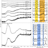 |
Fig. 1 Spectra of all discs considered in this study. The fluxes have been rescaled with respect to distance and |


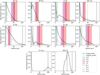 |
Fig. 2 Radial profiles of the disc sample based on the analysis in the image (black line) and visibility plane (grey line). The snowline estimates of H2O, CO2, CH4, and CO are indicated by the coloured areas. The minimum distance from the star that can be imaged, based on half the beam radius, is indicated by the hatched area. The Rgap , or the location of the innermost detected local minimum, is indicated by the vertical dotted line. The discs are organised from strongest |

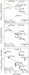 |
Fig. 3 Average of integrated line fluxes of warm (top, orange) and cold (middle, blue) H2O gas, and their ratio (bottom, black), plotted against the outer dust disc radius. The PCCs and p values for these log-log scatter plots are given in the panels, and the corresponding trend is indicated by the dotted black line. Upper and lower limits are indicated by triangles. |
3.3.2 C2H2
In the following sections, we compare the emission of the carbon species between rescaled DR Tau and the other discs. This comparison can be found in Fig. 6. First, we look at the left-most column, showing the C2H2 and 13C12CH2 emission, highlighted in yellow.
DR Tau itself shows clear C2H2 emission, but its isotopologue is dominated by an H2O line. It has neither the strongest, nor the weakest C2H2 emission in the sample, compared to the warm H2O emission. IQ Tau, Sz 98, and BP Tau are weaker in C2H2. SY Cha and potentially PDS 70 (although this source is quite noisy and C2H2 is not considered detected) are similar in their C2H2. CI Tau and GW Lup on the other hand, are slightly elevated compared to DR Tau though this difference is very small. Finally, both V1094 Sco and DL Tau show significant enhancement in C2H2. The 13C12CH2 feature, highlighted in yellow, overlaps with H2O, but the emission from H2O is weaker in these discs. Therefore, the emission in this region is more likely to originate from 13C12CH2, indicating the C2H2 emission is not just elevated, but also high in column density.
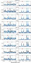 |
Fig. 4 Comparison of warm (indicated by the red triangle) and cold (indicated by the blue triangle) H2O lines between DR Tau rescaled to the line strength of the other discs (blue line), and the emission from the discs themselves (black line). |
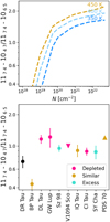 |
Fig. 5 Line flux ratio of the column density tracer from slab models (top), and the same line pair ratio in the spectra (bottom). The colourcoding corresponds to the observed depletion and excesses in colder H2O compared to DR Tau (black point), where similar emission properties to DR Tau are indicated with gold markers, an excess cyan markers, and a depletion pink markers. In the top plot, the temperature effects on the line flux ratio are demonstrated. In V1094 Sco and PDS 70 we do not detect one of the lines of the cold pair. Therefore, the lower/upper limits are indicated by the triangles in the bottom panel. |
3.3.3 HCN
The second and third columns show the HCN Q-branch and the hot branch. Again, DR Tau is neither exceptionally strong nor exceptionally weak compared to the other discs. Discs that are weaker in HCN are Sz 98, BP Tau, and to a lesser degree PDS 70 (once more limited by noise) and SY Cha. IQ Tau, GW Lup, and CI Tau are the same as DR Tau, whereas DL Tau and V1094 Sco are elevated in HCN. However, the HCN feature is blended with C2H2, so for DL Tau and V1094 Sco some of the peaks are affected by the strong C2H2 present in the spectrum. However, for the integrated line fluxes, this is mitigated by subtracting C2H2 slab model fits.
Overall, a strong detection of C2H2 coincides with detectable HCN, but HCN is more widely detectable than C2H2. For most discs, the HCN feature is stronger than C2H2, except for the very carbon-rich DL Tau and V1094 Sco, where C2H2 is brighter.
3.3.4 CO2
Finally, the three columns on the right of the figure demonstrate the emission of the CO2 Q-branch, 13CO2, and the CO2 hot branch, respectively. The detection of 13CO2, and a CO2 hot branch with a relatively bright peak compared to the main Q-branch shortward of 16.2 µm are indicators for elevated column densities (clear examples of both can be seen in GW Lup, as has also been discussed by Grant et al. 2023).
In terms of the Q-branch, several sources appear similar to DR Tau: SY Cha, BP Tau, Sz 98, CI Tau, and DL Tau. Sz 98 may have an enhanced column density, since its spectrum shows stronger emission from the hot branch compared to the main Q-branch. Similarly, IQ Tau is weaker in the Q-branch, but stronger in the hot branch, which indicates that its CO2 emission originates from a smaller emitting area, but with a higher column density. Finally, the other sources are enhanced in CO2. These include PDS 70 (although its spectrum is noisy due to the faintness of the source), GW Lup, and V1094 Sco. For the latter, the 13CO2 seems to also be detectable, indicating a high column density, similarly to GW Lup.
3.3.5 Carbon versus H2O
The comparisons above give an idea of the emitting strength of the carbon-bearing species compared to the warm H2O, since that is the measure on which the DR Tau rescaling is based. However, a comparison to the cooler H2O reservoir is also of interest, in particular whether a trend can be seen between an excess of cooler H2O, a potential indication for H2O-ice transportation, and the strength of the carbon emission. The line fluxes of the carbon-bearing species measured in the manner discussed in Sect. 2.3 can be found in Table A.3. Similarly to the H2O line fluxes, these are only normalised to the common distance, but not scaled by Lacc. The comparison to the H2O line fluxes is shown in Fig. 7, where the same colour-coding is used as in Fig. 5. The left column shows the flux ratios with H2Owarm, and the right column the ratios with H2Ocold. The windows over which the fluxes are calculated are mentioned in Sect. 2.3.
First, no dichotomy appears in the ratios with H2Owarm between the sources that are depleted or enhanced in H2Ocold. Generally, only two of the depleted sources are stronger in carbon emission compared to the warmer H2O: DL Tau and V1094 Sco.
On the other hand, a split occurs between the samples for the ratio with colder H2O. The depleted sources are stronger in carbon, especially HCN and C2H2, while the other discs are more centred near the bottom of the plots. The two sources that appear even more enhanced in H2Ocold also have very weak, if at all detectable, C2H2. The only sources that are not always split well from the depleted sources are PDS 70, which is not a full disc, and IQ Tau, which appears relatively strong in HCN. The latter could also be due to the weak colder H2O in IQ Tau. However, in general the discs depleted in cold H2O show stronger emission from carbon-bearing species.
4 Discussion
4.1 Inner disc emission and outer dust disc structure
In Sect. 3, we discussed the inner disc emission of the sample. A summary of the results can be found in Table 4. Despite the presence of substructures in all discs, some discs are H2O dominated and show signs of active dust migration, whereas others are much more carbon-rich. Based on modelling works, we identify different scenarios and try to put the observed emission into context, and illustrate these in Fig. 8. Before we discuss the discs in this sample in the context of the diagram, we first take the reader through the different scenarios based on the different models considered. We note that in all of these, a two population dust distribution is assumed, where some of the small dust is allowed to leak through the gap, independent of what happens to the pebbles. In this context, assumptions are made related to how much ice is carried by these small grains and how much can leak through the gaps, both of which are likely underestimated due to the simplified representation of the dust population. The scenarios discussed below and presented in Fig. 8 are directly based on these models, but this caveat must be kept in mind.
If the substructures are very leaky to dust pebbles, and therefore shallow, we can expect the disc evolution to progress similarly to a full, gap-free, viscous disc (e.g. Booth & Ilee 2019; Mah et al. 2024). This corresponds to scenario 1, where ices on dust pebbles are drifting in first, where ice species subsequently sublimate into the gas at their respective snowlines and no longer migrate inwards at the same rate as the pebbles. Therefore, the inner disc first becomes enriched in H2O (and we expect to be able to observe colder H2O out to the snowline), after which gases from the outer disc find their way inwards and the disc becomes enriched in CO2, and subsequently other carbon-bearing species. The majority of the H2O emission may appear hotter as it is accreted onto the star.
If a gap is only somewhat leaky to dust pebbles, it is a ‘moderate’ gap, and the inflow of dust is more regulated. This corresponds to scenarios 2 (close-in gap) and 3 (far out gap) in the figure, where some flux of pebbles is still able to cross the gaps. In the models of Mah et al. (2024), this results in significantly prolonged H2O-enrichment phases (and colder H2O), since the rate at which the dust moves into the inner disc is somewhat reduced. The outer disc would not run out of these grains as quickly. Based on Kalyaan et al. (2021, 2023), and Sellek et al. (2025), we observe that a deep gap closer to the star is more effective at blocking dust pebbles compared to scenario 3, as there simply is more dust starting outside of the gap. Therefore, the difference between scenarios 2 (close-by gap) and 3 (gap farther away) is that in scenario 2 the H2O enrichment period may last longer compared to scenario 3, longer than 10 Myr in the models of Mah et al. (2024).
If the gap is capable of blocking most, if not all, of the dust pebbles, it is a deep gap. In the models discussed, this can be caused by either planet formation-like mechanisms, or photoevaporation. The former is shown in scenarios 4 (close-in gap) and 5 (far out gap). In these cases, gas is allowed to diffuse across the gaps, but pebble drift is completely prevented. Realistically, in these cases the strong pressure bump can fragment the pebbles into smaller dust grains, in which case the dust can continue to migrate with the gas. If the gap is then located closer to the star, the dust reservoir inside the radius of the gap is quickly depleted, and the H2O enrichment phase is very short. The visible colder H2O emission quickly disappears, perhaps after less than a million years (Mah et al. 2024). On the other hand, a gap farther from the star is capable of blocking less dust, and the enrichment phase would last longer.
If photoevaporation processes are the cause of the gap, small dust grains and gas are also prevented from crossing the gap. This is illustrated in scenarios 6 (inside CO2 snowline) and 7 (outside CO2 snowline). Photoevaporative winds blow the gas out of the gap (Lienert et al. 2024). Contrary to all aforementioned scenarios, the cold H2O reservoir is continuously replenished. The gas in the inner disc diffuses outward towards the photoevaporative zone. If this zone lies outside the H2O snowline, but inside the snowlines of CO, CO2, and CH4, the H2O gas is able to condense back onto the dust and is carried inwards, while the other gases are lost to the photoevaporative zone (Lienert et al. 2024). However, this phase quickly results in a large cavity, depending on the viscosity of the disc, and occurs towards the end of the gas disc’s lifetime. Therefore, while an important scenario to keep in mind, it is unlikely that any of the discs presented here are exactly in the gap-opening phase.
An extended discussion of the individual discs in the context of Fig. 8 is included in Appendix B. The most important points are summarised here. Of the discs that show no cold H2O excess (see Table 4), only two discs (GW Lup and IQ Tau) have no gap inside the snowlines. For these discs we find evolved versions of scenarios 3 and 5 more likely. In contrast, if the substructures closer to the star are indeed deep enough to effectively block dust pebbles, V1094 Sco, DL Tau, and CI Tau may be examples of an evolved scenario 4. Of the sources with some cold H2O emission, DR Tau and Sz 98 show substructures within the snowlines. These discs may be examples of scenario 2, where the close gaps are not blocking all incoming dust pebbles. Since Sz 98 has a larger excess in cold H2O than DR Tau, more H2O-ice may be crossing the snowline. Furthermore, Sz 98 is much weaker in C2H2 and HCN compared to the other discs, which may correspond to scenario 6, though, as was mentioned above, it is unlikely to observe a system exactly in the gap-opening phase. IQ Tau falls somewhere between the cold H2O enhanced and depleted discs, and may be more evolved versions of scenarios 1 and 2.
The substructure identified in BP Tau is a cavity of a few astronomical units. Such a cavity may influence the inner disc emission, either due to gas depletion (e.g. Banzatti et al. 2017) or heating of the inner cavity wall (Vlasblom et al. 2024). In this case, the snowlines may be shifted outwards, resulting in enhanced H2O flux. Due to the cavity, it is difficult to place BP Tau in the context of Fig. 8. However, it may act most closely to scenario 1, since it lacks in detectable strong substructures aside from the cavity.
Discs with a very deep, extended gap (PDS 70 and SY Cha), are stronger in H2O emission than the carbon species. H2O is still present in PDS 70 and SY Cha, which indicates that some gas and dust is still reaching the inner disc across their large deep gaps. This is especially interesting in the case of SY Cha, which shows a stronger excess in cold H2O than DR Tau, indicating its emission is more drift-dominated, which is in line with the detection of gas within its gap (Orihara et al. 2023). This dust may not be larger pebbles, as is typically discussed in the models and when considering dust drift, but smaller dust grains moving inwards along with the gas. These smaller dust grains may still carry enough ices to replenish the inner disc in H2O, and other species, as is also discussed in Perotti et al. (2023), Pinilla et al. (2024), and Jang et al. (2024). In this case all scenarios from 1 to 5 may be valid, since small dust rather than pebbles bring the ices to the inner disc. Whether this is more universally happening in this type of disc, or whether SY Cha and PDS 70 are exceptions remains to be seen. An overview of the gas emission in transition discs will be available in Perotti et al. (in prep.).
Evidence for a variety of scenarios is found, but more data is needed to identify whether gaps truly have a significant impact on the inner disc composition, and which scenarios are most prevalent. Regardless, H2O-rich scenarios exist even in the presence of seemingly deep gaps, indicating that these substructures do not seem capable of fully blocking replenishment by ices or gases. This relates back to the aforementioned caveat, and it is important to consider the contribution of small dust to the ice being brought into the inner disc in the future. Furthermore, there may be differences in how much replenishment happens. Constraining the exact abundance of the gas species in the inner disc (by means of e.g.  detections, or optically thin lines with lower Aul) is therefore paramount.
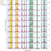 |
Fig. 6 Continuum-subtracted spectra, zoomed in on C2H2 and 13C12CH2 (left-most column), the HCN Q-branch and hot branch (second column and third column), the CO2 Q-branch, 13CO2, and CO2 hot branch (fourth, fifth, and sixth column). The respective features are highlighted in yellow, orange, or green, and prominent H2O features are highlighted in blue. The spectra are once more ordered from largest to smallest |

Summary of the emission per disc, mostly compared to DR Tau.
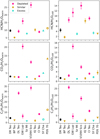 |
Fig. 7 Ratio of line fluxes of carbon-bearing molecules and warm (left) and cold (right) H2O. The colour coding follows that of Fig. 5: the discs indicated by a gold marker show similar cold H2O emission as DR Tau, cyan an excess, and pink a depletion. An open marker indicates a non-detection in both the carbon and H2O lines examined, whereas the triangles indicate lower or upper limits due to non-detections. |
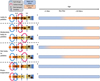 |
Fig. 8 Emission properties of the inner disc based on the modelling works by Kalyaan et al. (2021), Kalyaan et al. (2023), Mah et al. (2024), Lienert et al. (2024), and Sellek et al. (2025). |
4.2 Volatile trapping in ices
The calculation of the snowlines often assumes no volatile trapping within the ices and of ices within refractories (Potapov et al. 2024), which results in the classical interpretation of the C/O ratio changes in different parts of the disc (e.g. Öberg et al. 2011). However, ices are likely not neatly organised and separated on the dust particles, and may be trapped within ices of other species that have their snowlines closer to the star, as is seen in protostellar envelopes (e.g. Boogert et al. 2015) and the edge-on disc HH 48 NE (Sturm et al. 2023). In the context of this work, trapping of volatiles within H2O ice is of particular interest, since this would make the locations of other snowlines relative to substructures of smaller influence, since a fraction of the volatiles can be trapped within ices. Therefore, when discussing volatile trapping, we mean trapping of volatiles within H2O ice.
This is examined by Ligterink et al. (2024) and Bergner et al. (2024) for discs, and causes the gaseous C/O ratio to be much less dependent on the radial location within the disc, up to the H2O snowline where most volatiles are released from the H2O ice. The volatile trapping was studied in a lab context by Collings et al. (2004), showing that a large fraction of the volatiles may be released at several temperature regimes. Certain species, such as the hydrocarbons including CH4, but also CO2, are expected to be mixed in with the H2O ice, moving their true desorption temperature to that of H2O ice, as they cannot be released unless the surrounding H2O is. Additionally, H2O ice may be trapped in refractories and can only be released at the 400 K sublimation temperature of, for example, silicates (e.g. Potapov et al. 2024). On the other hand, CO ice is more apolar (Pontoppidan 2006), and likely a large fraction of the CO ice is free to be released into the gas at its own sublimation temperature (Collings et al. 2004).
While CO may not be efficiently trapped, it can be chemically processed into other ices on the timescale of a few million years in discs around T Tauri stars (e.g. Bosman et al. 2018; Krijt et al. 2020). In the cold environment of the outer disc, CO ice is processed into CO2 and CH3OH ice. Especially the former two ice species reach their sublimation temperatures much closer to the star, similarly to H2O, resulting in a similar effect as volatile trapping of CO itself would have.
This indicates that, similarly to the discussion in Ligterink et al. (2024), the composition of the gas and solids can be relatively constant throughout the outer disc, until the H2O and CO2 snowlines are reached. The location of the gaps relative to the snowlines, as was previously calculated, may therefore be of little consequence, unless they are inside the H2O and CO2 snowlines. A large part of the major carbon carriers is either trapped in H2O ice and brought in at the same time as H2O, or reprocessed into CO2 and CH3OH. Rather than reaching the inner disc later due to slower transport of gases, as is typically assumed for viscous, full disc evolution, they remain attached to the dust for longer and reach the inner disc simultaneously. Some progression from an oxygen-rich towards a more carbon-rich inner disc may still occur, since the outer disc gases that are there do tend to be more carbon-rich, but the notion of more carbon-rich species being left behind at their respective snowlines becomes less applicable.
The discs with the CO and CH4 snowlines outside some of their detectable substructures, like DR Tau, Sz 98, CI Tau, DL Tau, and V1094 Sco, may therefore experience not only the regulation in the influx of H2O, but in fact of many of the carbon species as well, just like the discs with the snowlines within their detectable substructures. The location of gaps with respect to how much material it can block in general (e.g. how much dust is present at larger radial distances) would matter more. In this case, a detectable colder H2O reservoir as a drift tracer would coincide with elevated emission in the other species as well. Therefore, the presence of a H2Ocold excess, in addition to considerable emission from the other molecular species discussed here, could be an indication of relatively ‘free’ viscous disc evolution. The lack of this H2Ocold excess, but clear emission from other species would indicate that most material being brought in is from the gas, and subsequently reprocessed through chemical reactions depending on the inner disc conditions, or very little radial transport occurs at all. The presence of an H2Ocold excess, but lack of emission from other species, would instead have to be a consequence of other processes dominating the inner disc emission, such as photoevaporation, the presence of a cavity, the entire disc having significantly different volatile ratios, or less trapping of ices.
4.3 Ages and formation timescales
For later stages of evolution to be reached, for example a more carbon-rich inner disc, the disc must be older, or the evolution timescale (as is dictated by the disc viscosity) relatively short. Constraining these properties would allow us to get a better understanding of what scenarios in Fig. 8 are more applicable. The inner disc composition can appear similar no matter how effective a gap is at blocking dust, if the evolution timescale is sufficiently slow, or the disc sufficiently young. As is modelled in Mah et al. (2024) and Sellek et al. (2025), the more viscous the disc, the faster its transport, and the faster different enhancement phases pass. Furthermore, more viscous discs contain more small dust grains, and substructures will generally be less effective at fully blocking dust, resulting in prolonged enrichment scenarios. On top of dust being less effectively blocked, the gas would also be transported inwards faster (Mah et al. 2024). If the silicate dust features in Fig. 1 are any indication of the abundance of small dust grains (Kessler-Silacci et al. 2006), the more peaked dust features exhibited by DR Tau, BP Tau, Sz 98, PDS 70, and SY Cha would hint at more small dust reaching the inner disc. This could be an indication of a higher disc viscosity and subsequently leakier gaps. The discs would then have to be relatively young to be able to retain the H2O excess they exhibit currently. However, dust grain sizes and the dust opacity are not stagnant and only dependent on the dust that is drifting inwards. These features may not allow us to distinguish between dust processing as is a natural occurrence for the discs, and the kind of dust that is reaching the inner disc.
Furthermore, as is also noted by Mah et al. (2024), for gaps to have a significant influence on the inner disc composition, they must form early in the disc lifetime. They propose that very deep gaps due to growing planets may only be possible to form early enough in very massive discs. Some of the more massive discs in this sample include V1094 Sco and DL Tau, both of which are poor in H2O. If their gaps are deep and did form early, this could have resulted in a quick passage of the H2O enriched phase resulting in the carbon-dominated discs we see now. However, planet formation is not the only mechanism that can carve gaps, and as has already discussed, the nature of the gap differs depending on what caused its formation (Bae et al. 2023; Lienert et al. 2024), although photoevaporation may only occur at very late stages of disc evolution.
4.4 Dust opacity
The hypothesis that disc substructures in the outer disc influence the inner disc composition, relies on transport of dust. Therefore, along with a delivery of oxygen-rich ices like H2O, dust is also moving into the inner disc. The consequences of this are discussed in Sellek et al. (2025), who show that this can also result in an increase in dust opacity, assuming the dust is coupled to the gas and a ‘traffic jam’ of grains occurs inside the H2O snowline. This increase in dust opacity may block the emission from gases closer to the midplane, resulting in the same column density of H2O gas emitting above the dust compared to before the grains drifted inwards, based on retrievals using synthetic spectra. They posit that the H2O emission properties and column density as probed by the mid-IR lines is a poor tracer of how much gas is actually present in the inner disc, due to this dust opacity increase. Even if the gas and dust are not coupled, the discs in the sample may have differences in dust opacity in the inner disc.
There have been some indications from models for certain species preferentially forming in different vertical layers of the disc (e.g. Woitke et al. 2018). Depending on where the dominant reservoirs of the different species are located, the differences in dust opacity of the discs in this sample could be influencing the emission that is visible in the MRS spectrum. More gas closer to the midplane could be obscured for one case, whereas another might be more transparent. The inner disc dust composition and abundance could therefore influence the species visible in the spectrum. Overall, the discs with flat-topped 10 µm silicate features (CI Tau, GW Lup, DL Tau, and V1094 Sco) show stronger emission from carbon-bearing species such as C2H2 and HCN, which would be in line with these molecules being located closer to the midplane than H2O.
4.5 Gas-to-dust ratio
Works that do not include migration of ices in their models are also able to reproduce the relative line fluxes of H2O and other species, such as HCN. The works of Antonellini et al. (2015) and Woitke et al. (2018), for example, show that the easiest way to achieve this is by increasing the gas-to-dust ratio or gas mass, where the former works somewhat like a reduced dust opacity, and the latter simply dictates whether there is enough gas present to produce detectable emission lines. Additionally, a more flared disc can be heated more by the central star, resulting in warmer and somewhat stronger emission from H2O in the MIRI/MRS wavelengths (Antonellini et al. 2015). The migration and processing of dust in general may be sufficient to produce enhancements of H2O fluxes and most other species, independent of the ices brought in by the dust (Antonellini et al. 2023). In this case, the H2O enhancement would still be age-dependent, but not dependent on the outer disc ice reservoir available for replenishment. This once more stresses the importance of accurate age estimates.
Greenwood et al. (2019) find C2H2 to not be affected by dust processing as strongly (demonstrated by their Fig. 9), even though we find a general increase in C2H2 flux for the discs with weaker H2O. Greenwood et al. (2019) also note this discrepancy with previous results from observations, and that their C2H2 emission behaves very differently from the emission of other species. They mention that these differences may be caused by missing formation pathways in the chemical network, or that their assumed dust models do not adequately describe the dust in C2H2 -rich discs. Antonellini et al. (2023) further argue that additional enrichment due to ices should not significantly affect the emission lines of H2O originating from the inner disc, which are in general optically thick already. However, the models in Temmink et al. (2024a) show that the coldest lines most dominant in the cold component are likely not optically thick, and can therefore further increase in flux with ice enhancement.
4.6 Gap depth and resolution
The proposal from the modelling side is that we may conclude how deep the gaps in the outer disc are or where they are located by comparing the inner disc composition to the expected composition from models (Mah et al. 2024). This is an interesting idea, and we note that the differences in distances to the objects and therefore the achievable resolution is varying in this sample. Some substructures that appear to be much deeper in one disc compared to the other, may simply be a result of a resolution difference. However, in our discussions above we have shown that there are currently too many uncertainties related to age, formation and transport timescales, volatile desorption, and gap properties as a result of formation mechanism preventing us from doing so with certainty. Instead, the reverse may be of interest, where the inner disc spectrum and visible outer disc structure can inform some of the aforementioned models, to see if the currently observable substructure is deep, shallow, or insufficient to explain the observed inner disc emission. This way it may also be possible to ascertain whether gaps that only block dust pebbles and not small dust grains or gas can even cause sufficiently different inner disc compositions, or whether the current notion of sequential snowlines is realistic. Interesting objects for these kinds of studies would be discs presented here that show some cold H2O excess and have deep gaps in millimetre wavelength. For example, Sz 98, which has a deep gap close to the star, but still shows indications for replenishment by H2O-ice. Furthermore, SY Cha has a gap of several tens of astronomical units, along with a cold H2O-excess. If transport of pebbles is blocked by these gaps, the influx of ices on small dust grains may also be able to cause this excess.
Furthermore, it it would be useful to identify whether the gaps in the dust continuum in this work are also gaps in the gas. To constrain this, we would need high resolution ALMA observations of CO isotopologues, as in van der Marel et al. (2016). If a gap exists in both the dust and the gas, it is likely that, in addition to pebbles, small dust grains and gas are also not able to reach the inner disc as quickly. In discs where this is the case, the inner disc spectrum may appear more depleted in many commonly detected species and in particular H2O, as was discussed above.
4.7 Implications for planet formation
It has been posited in the past that the C/O ratio of a planet can be traced back to where it formed in the disc, due to natural changes in the C/O ratio at different radial positions from the star (Öberg et al. 2011). However, as was noted previously, this sequence in snowlines may not be entirely representative of reality where volatiles may be trapped in H2O ice (Collings et al. 2004; Ligterink et al. 2024). So far, a planet’s atmospheric C/O has proven to be a poor tracer, due to phases of migration and other assumptions regarding a planet’s formation history and partitioning between the planet envelope and core changing the resulting C/O (see e.g. Mordasini et al. 2016; Mollière et al. 2022), and more tracers are now being taken into account (e.g. Pacetti et al. 2022). Furthermore, the atmospheric C/O may not be representative for the planet’s bulk C/O. Nevertheless, the species available at the time of accretion do dictate a planet’s resulting composition.
In Sect. 4.1, we note that the presence of substructures within the CO and CH4 snowlines may reduce the gaseous C/O ratio in the inner disc, if gas diffusion across the gap is inhibited, such as for photoevaporation. On the other hand, if volatiles are trapped, the presence of a gap outside the H2O snowline may prevent replenishment of oxygen in general, and the carbon rich, but overall depleted, gas can still reach the inner disc to increase its C/O. While it is unlikely that planet formation completely cuts off the inner disc from the influence of the outer disc, be it dust or gas transport, if some transport is moderated sufficiently early, planets forming in the inner disc can be more significantly replenished in H2O. Whether or not the location of the outer planet matters compared to the different snowlines depends on whether there is actually a sequence in sublimation of ices, or if most of the CO2, CO, and CH4 can be trapped in H2O ice.
Van der Marel et al. (2021) also found that the presence of a gap influences the C/O and C/H ratios in the outer disc. It is therefore possible that a giant outer planet, massive enough to carve a gap in the disc, could influence the formation conditions in the inner disc. This might bring to mind our Solar System, where Jupiter could have been this giant planet carving a gap (Morbidelli et al. 2016; Haugbølle et al. 2019), and Earth could have been a planet forming in the inner disc influenced by this. In fact, Jupiter has been dated to have formed early in the Solar System’s evolution (Kruijer et al. 2017), though this would have reportedly blocked H2O-ice and resulted in a ‘dry’ inner disc. Instead, we propose that, while eventually the inner disc may dry out, the presence of a gap within the snowlines of the major carbon carriers may rather regulate the amount of incoming dust grains and pebbles, allowing for a somewhat enhanced H2O abundance in the inner disc over extended timescales. Therefore, a planet in the outer disc may instead allow for prolonged formation of water-rich worlds in the inner disc, when he outer gas giant forms sufficiently early in the disc lifetime.
5 Conclusion
In this work, we aim to link the outer dust disc structure to the inner disc gas composition, based on ALMA and MIRI/MRS, respectively. Modelling efforts show clear indications of the influence of substructures on the H2O enhancement and volatile C/O ratio, but also on the timescales for which these enhancement scenarios last.
The sample of 10 discs presented here shows quite some variation in inner disc emission and outer disc structure. Overall, transport does not seem to be fully prevented. SY Cha and PDS 70 contain deep, wide gaps that are not fully devoid of gas. This is reflected in their inner disc composition, where SY Cha especially shows a strong cold H2O excess. Similarly, Sz 98 has one of the deepest gaps close to the star in the sample, and also shows a clear cold H2O excess. Perhaps the gaps are able to stop the pebbles from reaching the inner disc, but the gas and small dust may still bring in a sufficient abundance of ices.
Furthermore, the discs that do not show a clear excess in a cold H2O reservoir show stronger emission from the carbon- bearing species, and vice versa. This is especially clear in C2H2 and HCN, but less so for CO2, which is likely influenced by other processes and still contains oxygen.
Two factors that are important to consider in future work are the uncertainties related to age and gap formation timescales and whether volatiles are mostly trapped in H2O ice or whether ices are reprocessed into species with higher binding energies. Both dictate whether the gap or its location with respect to the H2O, CO2, and CO snowlines truly have an influence on the inner disc composition.
Acknowledgements
We thank Andrea Banzatti for useful discussions related to the line selection for the water spectrum, and Feng Long for sharing the DL Tau continuum measurement set. We also thank the anonymous referee for their thorough and useful feedback. This work is based on observations made with the NASA/ESA/CSA James Webb Space Telescope. The data were obtained from the Mikulski Archive for Space Telescopes at the Space Telescope Science Institute, which is operated by the Association of Universities for Research in Astronomy, Inc., under NASA contract NAS 5-03127 for JWST. These observations are associated with programmes #1282 and #1640. This paper makes use of the following ALMA data: ADS/JAO.ALMA#2016.1.00484.L, ADS/JAO.ALMA#2016.1.01164.S, ADS/JAO.ALMA#2016.1.01370.S, ADS/JAO.ALMA#2017.1.01167.S, ADS/JAO.ALMA#2018.1.01458.S, ADS/JAO.ALMA#2019.1.00607.S. ALMA is a partnership of ESO (representing its member states), NSF (USA) and NINS (Japan), together with NRC (Canada), NSTC and ASIAA (Taiwan), and KASI (Republic of Korea), in cooperation with the Republic of Chile. The Joint ALMA Observatory is operated by ESO, AUI/NRAO and NAOJ. The project leading to this publication has received support from ORP, that is funded by the European Union’s Horizon 2020 research and innovation programme under grant agreement No 101004719 [ORP]. A.C.G. acknowledges support from PRIN-MUR 2022 20228JPA3A “The path to star and planet formation in the JWST era (PATH)” funded by NextGeneration EU and by INAF-GoG 2022 “NIR-dark Accretion Outbursts in Massive Young stellar objects (NAOMY)” and Large Grant INAF 2022 “YSOs Outflows, discs and Accretion: towards a global framework for the evolution of planet forming systems (YODA)”. G.P. gratefully acknowledges support from the Carlsberg Foundation, grant CF23-0481 and from the Max Planck Society. E.v.D. acknowledges support from the ERC grant 101019751 MOLDISK and the Danish National Research Foundation through the Center of Excellence “InterCat” (DNRF150). T.H. and K.S. acknowledge support from the European Research Council under the Horizon 2020 Framework Program via the ERC Advanced Grant Origins 83 24 28. I.K., A.M.A., and E.v.D. acknowledge support from grant TOP-1 614.001.751 from the Dutch Research Council (NWO). I.K., J.K., and T.K. acknowledge funding from H2020-MSCA-ITN-2019, grant no. 860470 (CHAMELEON). B.T. is a Laureate of the Paris Region fellowship program, which is supported by the Ile-de-France Region and has received funding under the Horizon 2020 innovation framework program and Marie Sklodowska-Curie grant agreement No. 945298. D.G. thanks the Belgian Federal Science Policy Office (BELSPO) for the provision of financial support in the framework of the PRODEX Programme of the European Space Agency (ESA). D.B. has been funded by Spanish MCIN/AEI/10.13039/501100011033 grants PID2019-107061GB-C61 and No. MDM-2017-0737. M.T. and M.V. acknowledge support from the ERC grant 101019751 MOLDISK.
Appendix A Selected H2O lines and line fluxes
In Fig. A.1 and Table A.1, we summarise the H2O lines that are considered in this study.
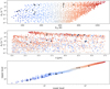 |
Fig. A.1 Lines used to calculate the warm and cold water line fluxes. The open circles are single lines. The open triangles are a line pair with the same upper level used to probe the column density in the cold water gas. |
Appendix B Extended discussion of scenarios per disc
B.1 DR Tau
We start this discussion with DR Tau, the most H2O-rich source in this sample by far, but only a marginal excess of cold H2O (Temmink et al. 2024a). Its age is estimated to be around 1.8 to 5.9 Myrs (see Table 1). It is certainly not the weakest in its emission strength of the carbon species, but not the strongest either. This likely places it in one of the H2O-rich scenarios of Fig. 8. Additionally, in Fig. 2 it can be seen that its dust disc is relatively small, with some weaker substructure at the current spatial resolution, with the CO and CH4 snowlines clearly outside of the inner-most substructure. Assuming its age is a few million years (see Table 1), these substructures are likely not completely blocking the incoming dust pebbles. If they were, the H2O in the inner disc might already have been depleted on these timescales. This leaves the possibilities of the shallow and moderate gaps (cases 1 and 2, respectively) to be more likely, with scenario 2 the most likely if the disc is on the older end of the age estimates.
B.2 BP Tau
As is mentioned in Table 1, the age of BP Tau is estimated to be in the range of 1.0 to 3.4 Myrs. The substructure identified in BP Tau is either a very close-in gap, or a cavity of a few astronomical units. Furthermore, in Table 4 it can be seen that it is likely somewhat depleted in carbon, but similar in oxygen to DR Tau. It could be that BP Tau is younger, resulting in more of its carbon-rich ices and gases still making their way inwards from the outer disc. Its H2Owarm line fluxes are weaker compared to its H2Ocold. According to Banzatti et al. (2017), the presence of some gas depletion in the inner disc could result in weaker warmer H2O. Rather than from the outside in, like dust migration inwards would cause, the H2O gas is depleted from the inside out. A similar effect is modelled in Vlasblom et al. (2024), where for cavity sizes of a few astronomical units like in BP Tau, first the H2O flux is increased compared to CO2. Initially, the snowlines are simply shifted outwards, increasing the flux of the molecular lines. Additionally, the accretion luminosity of BP Tau indicates that, while it is on the lower end in the sample, material is still being accreted onto the star, meaning the cavity is not completely void of material. Vlasblom et al. (2024) show that in this case, the increase in relative CO2 flux becomes less prominent as well. Due to the potential presence of the inner cavity of a few astronomical units, BP Tau may not fall under any of the categories shown in Fig. 8, although its evolution may be similar to scenario 1, depending on how the cavity evolves.
Summary of H2O lines with quantum numbers 000–000 (v1v2v3, upper-lower levels) used in this work.
B.3 Sz 98
The age of Sz 98 has quite a wide estimated range (as is mentioned in Table 1), but we assume it is similar to the other discs in this sample; of the order of a few million years. As is presented in Table 4, Sz 98 may be somewhat enhanced in oxygen compared to DR Tau. It is bright in H2O and may have a somewhat higher column density of CO2 than DR Tau, but it appears weaker in the other carbon bearing species, especially C2H2. Additionally, based on its profile in Fig. 2, we observe that its disc contains a strong substructure near the star, inside the snowlines of CO and CH4. Similarly to DR Tau, if it is of the order of a few million years old, this inner gap should result in relatively quick depletion of H2O if it were blocking all the dust. Since this is not the case, we might expect it to fall under the shallow and moderate gap categories, like DR Tau. However, in this scenario the carbon-rich gases from the outer disc could still freely move towards the inner disc. Since the spectrum of the inner disc presents itself as relatively carbon-poor, either this has not yet happened, or the gas is also blocked from reaching the inner disc. In this case, the gap may instead be caused by photoevaporation, rather than processes akin to planet formation. In case 6 or 7 of Fig. 8, the inner disc quickly becomes H2O rich as the carbon grains and gases are completely blocked from reaching the inner disc. In addition, the gas in the inner disc is spread back outward across the H2O snowline, and H2O can migrate back as ice across its snowline. This results in a long H2O equilibrium cycle (Lienert et al. 2024), where the inner disc becomes H2O rich and carbon poor, and we can observe a cold H2O reservoir for extended periods of time. However, this requires a low viscosity to maintain the inner disc for an extended period of time.
B.4 IQ Tau
Interestingly, the outer disc structure of IQ Tau appears quite similar to that of DR Tau (see Fig. 2). The age estimates are also not dissimilar, with estimates ranging from 2.2 to 8.3 Myrs (see Table 1). It shows some of the stronger H2O line fluxes in the sample, especially in terms of its warmer reservoir. In Sect. 3 we observed that its colder H2O reservoir is weaker than DR Tau in terms of emission strength, but the relative strength of the first and third line in the 23.8-24 µm quadruplet indicates that some excess H2 Ocold may be present, albeit on the weaker end in the sample. Furthermore, its C2H2 and CO2 Q-branch emission appears weaker than DR Tau. The excess in the range of the hot branch of CO2 may point towards a higher column density, but due to the relatively weak CO2 Q-branch it is more likely that this is more strengthened by an H2O line in this range. Its luminosity is lower than DR Tau, which may have two consequences. First, the temperatures may be lower in the inner disc, resulting in CO2 formation being favoured over H2O formation, and therefore in a higher column density for the former (e.g. Woitke et al. 2009; Glassgold et al. 2009; van Dishoeck et al. 2013). Due to the weak Q-branch, this may be less realistic. Second, the distance between the star and the H2O snowline reduces, in turn reducing the possible emitting area for the colder H2O reservoir. Based on the estimated snowline location in Fig. 2, it could be that the emitting area of H2O, and especially the H2 Ocold, may simply be less than in DR Tau. Furthermore, due to this lower luminosity, the CO and CH4 snowlines are within the detected substructures in IQ Tau. These substructures may be leaky to dust as suspected for DR Tau, and IQ Tau may be moving from the younger versions of scenarios 1 or 2, to a more processed, more CO2 rich disc as is shown in Fig. 8, and modelled in Sellek et al. (2025).
B.5 CI Tau
The disc structure shown in Fig. 2 of CI Tau shows similarities to Sz 98, with a deep gap relatively close to the star. Its age is estimated to be on the 1.4 to 4.5 Myr range (Table 1). Contrary to Sz 98, however, it is stronger in C2H2, much less so in H2Ocold, and similar to DR Tau in all other examined emission (see Table 4). While the colder H2O reservoir may be smaller, its warmer H2O is still relatively strong in the sample. Therefore, CI Tau may be in the process of accreting its H2O gas and relatively little may be coming in. In that case, the detected most dominant H2O emission is from a warmer reservoir closer to the star, where the outer regions closer to the snowline are slowly depleted of H2O. This would indicate that its inner gap is relatively deep, corresponding to scenario 4 in Fig. 8, allowing this phase to start earlier than for DR Tau, whose gap may be leakier. Similarly to Sz 98, the CO and CH4 snowlines are clearly outside of the most prominent substructure, yet its inner disc does not seem to be significantly depleted in carbon. This, along with the lack of a strong cold H2O signature, would exclude photoevaporation gaps, as opposed to Sz 98. The only other significant difference with Sz 98 is the stellar luminosity, which is significantly lower than Sz 98.
B.6 GW Lup
As is mentioned in Table 1, the age of GW Lup is estimated to be from 0.8 to 5.0 Myrs. GW Lup is extremely strong in CO2, high in the sample in its warmer H2O emission, but seemingly depleted in cold H2O. Furthermore, its strongest substructure appears relatively far from the star, around 74 au (see Fig. 2 and Appendix C), several very weak substructures in the radial profile appear closer to the star, but these are by far the weakest variations in the sample. The strongest gap may be too far out to block a significant part of the H2O ices from reaching the inner disc (Kalyaan et al. 2021, 2023). This would point to scenarios 3 and 5 in Fig. 8 being more likely. The H2Owarm is stronger than H2Ocold, indicating the H2O reservoir is no longer strongly being replenished, and in the process of accreting onto the star. In turn, the disc is in the CO2 enhanced phase (Sellek et al. 2025), as is indicated by the strong CO2 emission and the detection of 13CO2. Therefore, more evolved cases of scenarios 3 and 5 are likely. Moreover, the luminosity of GW Lup is relatively low in this sample, and may therefore, similarly to IQ Tau, have its snowlines closer to the star, allowing them to reach a more evolved stage more rapidly.
B.7 DL Tau
The age of DL Tau is estimated to fall between 1.9 to 6.3 Myrs (Table 1). DL Tau is one of the weakest H2O emitters out of the full discs presented in this sample, and does not appear significantly stronger in its CO2 emission. It is therefore unlikely that a significant portion of its oxygen is locked up in CO2 rather than H2O. Its HCN and C2H2 emission on the other hand, we show to be comparatively much stronger, as summarised in Table 4. The inner disc therefore appears relatively depleted in oxygen, and enhanced in carbon. The relatively warm remaining H2O reservoir indicates the emission may originate from closer to the star, and not out to the snowline. Its radial profile in Fig. 2 shows a range of relatively shallow substructures, with one deeper gap present around 60 au. Similarly to GW Lup, this gap farther out may not be as effective at blocking H2O ice, allowing for evolution closer to scenarios 1, 3 or 5, in a more evolved stage of its lifetime. Alternatively, the gap closer to the star could be very deep, in which case the disc can be younger, as its H2O rich phase would pass after less than a million years (Mah et al. 2024).
B.8 V1094 Sco
The final full disc, V1094 Sco, has even larger uncertainties in its age compared to Sz 98 (see Table 1 and the related note). It has the lowest H2O flux overall in this sample, and it likely does not contain an exceptionally strong cold H2O reservoir. It is much stronger in C2H2, HCN, and CO2, as is shown in Table 3. However, its CO2 is not as strong as in GW Lup, which, along with the strength of the other carbon species, indicates that the inner disc might have a relatively high C/O. Taking a look at its outer disc structure then, in Fig. 2, it can be seen that the most prominent substructure is located relatively close to the star, around 17 au. This gap may be deep, resulting in an evolved scenario 4, where the H2O enhanced phase very rapidly passes and the inner disc quickly presents itself as more carbon-rich. Since the CO and CH4 snowlines are present outside this inner substructure, it is likely that the carbon gases are able to freely migrate across the gap. Alternatively, if the gap is shallow (scenario 1) or moderate (scenario 2), the disc must be older (Mah et al. 2024). For the shallow case this means likely older than a few million years, which seems feasible, but for the moderate gap this may mean an age of well over 10 Myrs, which may be less realistic.
B.9 SY Cha
The estimated age of SY Cha is 3 Myrs, as was previously mentioned in Table 1). Out of the two discs with extremely wide gaps, SY Cha clearly has the strongest in H2O emission, and indeed all molecular emission overall, as is also discussed in Schwarz et al. (2024). In fact, while its warm H2O lines are not always confidently detected, the strength of the detected cold H2O lines is the highest overall. Along with Sz 98, it is the only source with indications for a more enhanced cold H2O reservoir. In all other species, it is similar to DR Tau as well. The inner disc of SY Cha is small and may itself have a smaller cavity near the star, whereas the deep cavity from the inner disc up to ~70 au is likely not fully depleted of gas (Orihara et al. 2023). The smaller H2Owarm flux may in this case have similar origins to BP Tau. SY Cha may be somewhat depleted in material close to the star, reducing the flux of the shorter wavelength, warmer lines (Banzatti et al. 2017; Banzatti et al. 2020). Additionally, the detection of gas within the deep outer cavity indicates that it is not stopping all material from flowing inwards. Especially carbon dominated gases can find their way inwards from the outer disc, along with some smaller dust grains coupled to the gas, which may be able to replenish some of the inner H2O reservoir, as is also proposed by Schwarz et al. (2024).
B.10 PDS 70
The story may be somewhat similar for PDS 70 to that of SY Cha, although PDS 70 is estimated to be slightly older than SY Cha (4.4 to 6.4 Myrs, versus 3 Myrs, Table 1). It is also a disc with a major gap of tens of astronomical units wide, and a relatively weak inner disc with a radius of 18 au (Benisty et al. 2021). The disc MRS spectrum, published in Perotti et al. (2023), shows some H2O emission, but very little, if any C2H2 and HCN, and perhaps an elevated CO2 flux compared to DR Tau. Again, the presence of the wide outer gap does not prevent the oxygen species from being more dominant in the inner disc, as is discussed in Perotti et al. (2023). Furthermore, Pinilla et al. (2024) and Jang et al. (2024) theorise that aside from some gas, small dust may also be moving from the outer disc to the inner disc, perhaps replenishing some of the inner disc’s oxygen. This is also in line with the observations in Perotti et al. (2023). In the case of PDS 70, the large gap may be more depleted and its oxygen replenishment may be less significant than for SY Cha, resulting in a more CO2 dominant disc, or it is simply older, similarly to some of the scenarios for the full discs as is shown in Fig. 8.
Appendix C Estimating radii and gaps from ALMA
C.1 ALMA observations
As we are interested in the substructures closest to the host star, we have retrieved all the highest available spatial resolution ALMA observations publicly available for our sources. We list the distances, inclinations, position angles, and some of the observation properties in Table C.1. As for many of the sources, except BP Tau, the inclination and the position angle are well constrained, we use the literature values while fitting the visibilities. For BP Tau, we estimated updated values using the CASA-task IMFIT by fitting an elliptical Gaussian. Additionally, we used IMFIT to estimate the phase offsets (∆α and Δδ, both in arcsec) for each source and corrected for these offsets using the CASA-task FIXVIS. For some sources (CI Tau and GW Lup), additional shifts were determined from the image plane, ensuring that the peak flux in the model falls on the same position as the peak flux in the image. For only three of our sources (CI Tau, DR Tau, and IQ Tau), self-calibration yielded an increased signal-to-noise ratios (S/N). Therefore, we performed two rounds of phase-only self-calibration (solution intervals of ‘inf’ and ‘30s’) for these sources. We have imaged (down to a threshold of 1.5 × the root-mean square) the dust continuum of all our sources using the ‘Briggs’ weighting scheme with a robust parameter of +0.5. Fig. C.1 displays the continuum images and the resolving beams are highlighted in Table C.1.
C.2 Visibility fitting
Given the non-uniformity of the ALMA sample, we have fitted the visibilities to infer potentially ‘hidden’ substructures in the discs that cannot be retrieved from the cleaned images. We have followed the approach by Zhang et al. (2016), where a Hankel transform acts as the link between the deprojected uv-distance and the radial brightness distribution (I(θ)) (Pearson 1999):
 (C.1)
(C.1)
 (C.2)
(C.2)
 (C.3)
(C.3)
Here, i and ф are the disc’s inclination and position,  denotes the deprojected uv-distance (given in units of λ, and θ is the radial angular scale as seen from the disc’s centre. Finally, J0 denotes the zeroth-order Bessel function of the first kinds. The model brightness distribution consists of a set of Gaussian functions, inspired by the peaks seen in the visibilities and modulated by a sinusoidal function that has a spatial frequency of ρi,
 (C.4)
(C.4)
Source properties and band 6 ALMA observations of the eight T Tauri discs.
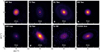 |
Fig. C.1 ALMA continuum images of the various sources. The resolving beams are displayed in the lower left corner and the horizontal bars indicate scales of 50 au. |
This function yields the {a0, σ0, ai, σi, ρi} as the set of free parameters. For our sample, we report the minimum of additional Gaussian functions that results in a good fit to all the visible features in the visibilities.
We have deprojected the visibilities using the inclinations and position angles listed in Table C.1. To ensure that we are able to fit the visibilities properly, we have visually compared the visibilities of all spectral windows (line and continuum) with those of the continuum spectral windows alone. For the line spectral windows, we masked visible lines, ensuring that they only contain continuum emission. In the cases of DR Tau, GW Lup, and Sz 98, we found that the uncertainties of the visibilities of the continuum spectral windows were significantly lower than those when including all spectral windows. Therefore, we only used the continuum spectral windows for those three sources. In addition, we only use the continuum spectral windows for DL Tau, as the measurement set was obtained through private communication. For all other sources we have used all spectral windows.
We bin the visibilities to speed up the fitting process, using the implementation of the FRANKENSTEIN-code (Jennings et al. 2020) and we avoid fitting the visibilities with large scatter, generally occurring at larger values of kλ. For BP Tau, DL Tau, DR Tau, Sz 98, and V1094 Sco we limit the visibilities to ≤2000 kλ, whereas we limit the visibilities of CI Tau and GW Lup to ≤3000 kλ. Finally, the visibilities of IQ Tau are limited to ≤1500 kλ. In addition, the visibilities are binned to widths of 1- 2×10⁴ λ; that is, the binned visibilities have widths of 1-2×10⁴ λ or 10-20 kλ. We fit the visibilities using the Markov Chain Monte Carlo (MCMC) implementation of the EMCEE-package (Foreman-Mackey et al. 2013). The fitting was performed twofold, similarly to the approach carried out by Long et al. (2018): in the first round, we used 2500 iterations to explore the prior space, identifying the best-fit parameters. In the second round, we used 10 000 iterations to explore a confined parameter space around these best-fit parameters. From this second round, we use a final 5000 iterations to identify the median values of the posterior distributions. The lower and upper uncertainties are, respectively, taken to be the 16th and 84th percentiles. Our fitting results are listed in Table C.2 and the fits to the visibilities are shown in Figure C.2.
C.3 Characterising the millimetre continuum emission
Using the radial brightness distribution from median values of the posterior distributions, we infer the radial locations of substructures. The locations of rings (rr) and gaps (rg) are identified through, respectively, the local maxima and minima present in the profiles. Other structures, such as ‘shoulders’ or ‘plateaus’, visible in the radial profiles are visually identified. To characterise the depth and widths of the identified gaps, we follow the approach of Huang et al. (2018). Here, the gap depth is defined as the ratio of the gap intensity (Ig) and that of the neighbouring ring with the smallest flux contrast (Ir), ∆Ig = Ig/1r. Given the ratio, the gaps with the smallest value reported for the depth are the deepest ones. The width of the gap is determined as the radial width between the inner and outer edges of the gaps (rg,i and rg,o), which are the radial locations where the intensity equals Imean = 0.5 (Ig + Ir). Therefore, the width is given by ∆rg = rg,o − rg,i.
We also determine the continuum disc radius (Rdisc) using a curve-of-growth method (see also Ansdell et al. 2016 and/or Stapper et al. 2022 for more information) for radii containing 68%, 90%, and 95% of the flux density. The values for the disc radii are listed in Table C.3. In short, we use aperture photometry to investigate at what radius the flux density within the apertures flattens off. We increase the apertures by the pixel size and limit our range to where we see no significant substructures in the ALMA radial profiles, as we are only using high-resolution observations, and therefore we may lack the resolving power for weak outer disc features.
The model radial profiles, together with the identified gaps and rings, are shown in Figure C.2. Here, we also show the ALMA continuum image and the model radial profile convolved with a Gaussian kernel tailored after the ALMA resolving beam. The convolved radial profiles clearly show that the beam is responsible for smoothing out weak structures in the ALMA image and, subsequently, that these features cannot be distinguished from the images. All the retrieved locations of the gaps and the rings, and the gap widths and depths are listed in Table C.3. Additionally, in Figure C.3 we display a comparison between the ALMA continuum image, the model image, the model image convolved with a Gaussian kernel, and the residuals. The residuals are obtained by subtracting the convolved model image off the ALMA image. Similarly to what is seen for the radial profiles, the convolution with the Gaussian kernel smooths out the various weak substructures visible in the model and therefore become unidentifiable in the images.
Besides the various gaps and rings, we also visually identified a few plateaus, which may hint at additional substructures. These plateaus are indicated by the red arrows in Figure C.2. To summarise, we identify three plateaus: in DR Tau at ~19 au, in GW Lup at ~ 17 au, and in IQ Tau at ~20 au.
Overall we find that the convolved images represent the ALMA images quite well, but there are some residuals that require attention. The residuals of BP Tau are mostly negative, indicating larger flux in the model image following the identified cavity in the models. The central, unresolved spot in the ALMA image may be attributed to free-free emission or emission from the host star itself (see e.g. Rota et al. 2024). For CI Tau, the residuals show that clear asymmetric structures are found in the ALMA image. These residuals show that the outer edges of the gap are not perfectly oval shaped as it is in the model. DL Tau, DR Tau, and IQ Tau all three show clear residuals in the central positions. These asymmetries likely arise from sub-pixel offsets between the peaks of the ALMA images and the model images. We note that the observations for these sources have the lowest spatial resolution (~0.11”), which provides a potential explanation why these residuals are the largest. Higher resolution observations will likely provide better fits and cleaner residuals. The residuals of GW Lup are dominated by the model overfitting the width of the inner region, as can also be seen from the radial profiles (see Figure C.2). Additionally, there may be a sub-pixel offset for the location of the maximum flux in the ALMA image, which causes the asymmetric feature to appear in the residuals. For both Sz 98 and V1094 Sco, we see that the residuals are rather patchy, which may be caused by the use of only the highest resolution observations available. Combining these observations with those of lower resolution, which are better at resolving the largest scales, may improve the residuals.
C.4 Comparison with previous works
Almost all of the discs, except Sz 98, have been modelled before, we compare the inferred substructures:
BP Tau: BP Tau has previously been fitted by Zhang et al. (2023), but no fits have been carried out for the high-resolution observations used in this work. We note that the models of Zhang et al. (2023) already point towards a small cavity in this disc, which now seems confirmed by our results. Additional analysis of this source will be presented in a future publication of the PI’s team.
CI Tau: The high-resolution CI Tau observations used in this work have previously been modelled by Clarke et al. (2018) and Rosotti et al. (2021). They find radial locations for the gaps of ~12, ~45, and ~114 au, and radii of ~23, ~54, and ~114 au for the rings. Generally, these values are close to our values, except for the outer most ring, for which we find a larger value of ~ 155 au.
DL Tau: DL Tau has been modelled by Zhang et al. (2023) using the same technique, but also has been given an extensive treatment by Jennings et al. (2022b). Both works yield similar radial brightness profiles. In addition, Zhang et al. (2023) lists gap locations of ~15, ~31, ~47, ~66, ~95, and ~129 au, which all fall within 10 au of our listed values. The fit by Zhang et al. (2023) suggests deeper gaps. As is seen in Figure C.2 our convolved profile does not fully match the ALMA profile, suggesting that our modelled rings are not as strong as those of Zhang et al. (2023), yielding smaller gap depths.
DR Tau: Similar to DL Tau, DR Tau has been modelled by Jennings et al. (2022b) and Zhang et al. (2023). Again, we find that the respective brightness profiles are rather similar, except we note that we find an additional potential substructure gap-ring combination at, respectively, 61.2 and 69.2 au. The other gaps are found at similar locations, although we find that the first gap identified by Zhang et al. (2023) (~ 18 au) appears as a plateau in our profile.
GW Lup: GW Lup was modelled by Jennings et al. (2022a), which finds a similar looking brightness profile, with a plateau in the inner regions (<0.1"). Overall, we find a few more potential substructures apart from the well-known ring at 86 au. As these substructures are not identified by Jennings et al. (2022a), we propose to treat these potential substructures with caution.
IQ Tau: IQ Tau has also been modelled by Zhang et al. (2023). We find the same location for the gap-ring combination around ~40 au. However, the outer two rings identified in our work are not found in their work. Therefore, we propose to treat these two potential substructures with caution. Higher spatial resolution observations may proof if these substructures do indeed exist or not.
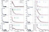 |
Fig. C.2 Fit to the visibilities (blue line in the left panels for each source) and the various radial profiles (right panels): one from the ALMA image (black line), the model radial profile (blue line), and the radial profile from the model convolved with a Gaussian kernel tailored after the resolving beam (red line). The shaded grey area indicates the standard deviation in each radial bin of the ALMA profile. The gaps and rings (or local minima and maxima) and plateaus/shoulders are indicated by, respectively, the blue, green, and red arrows, where the values indicate their integer radial positions. The location of the innermost gap is emphasised by the dark blue arrows. |
V1094 Sco: These higher resolution observations of V1094 Sco have not been modelled before, but van Terwisga et al. (2018) modelled lower resolution (~0.18”) observations. They only provided locations for gaps located at 100 and 170 au. Our fit to the higher resolution observations thus provide hints for potentially more substructures, with the most notable gap at ~16 au.
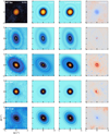 |
Fig. C.3 Comparison between the ALMA image (first column), the model image (second column), the convolved model (third column), and the residuals (final column). All images, except the residuals, are shown with an arcsinh-stretch colourmap. The residuals are taken by subtracting the convolved model image off the ALMA image. Here, red residuals indicate more flux in the ALMA image, whereas blue residuals indicate more flux in the convolved model image. |
Median values from the fitting posterior distributions and the corresponding uncertainties.
Identified substructures and dust continuum sizes for the sources.
References
- Alcalá, J. M., Manara, C. F., Natta, A., et al. 2017, A&A, 600, A20 [NASA ADS] [CrossRef] [EDP Sciences] [Google Scholar]
- Alexander, R., Pascucci, I., Andrews, S., Armitage, P., & Cieza, L. 2014, in Protostars and Planets VI, eds. H. Beuther, R. S. Klessen, C. P. Dullemond, & T. Henning, 475 [Google Scholar]
- ALMA Partnership (Brogan, C. L., et al.) 2015, ApJ, 808, L3 [Google Scholar]
- Andrews, S. M., Huang, J., Pérez, L. M., et al. 2018, ApJ, 869, L41 [NASA ADS] [CrossRef] [Google Scholar]
- Ansdell, M., Williams, J. P., van der Marel, N., et al. 2016, ApJ, 828, 46 [Google Scholar]
- Antonellini, S., Kamp, I., Riviere-Marichalar, P., et al. 2015, A&A, 582, A105 [NASA ADS] [CrossRef] [EDP Sciences] [Google Scholar]
- Antonellini, S., Kamp, I., & Waters, L. B. F. M. 2023, A&A, 672, A92 [NASA ADS] [CrossRef] [EDP Sciences] [Google Scholar]
- Arabhavi, A. M., Kamp, I., Henning, T., et al. 2024, Science, 384, 1086 [NASA ADS] [CrossRef] [Google Scholar]
- Argyriou, I., Glasse, A., Law, D. R., et al. 2023, A&A, 675, A111 [NASA ADS] [CrossRef] [EDP Sciences] [Google Scholar]
- Bae, J., Isella, A., Zhu, Z., et al. 2023, in Astronomical Society of the Pacific Conference Series, 534, Protostars and Planets VII, eds. S. Inutsuka, Y. Aikawa, T. Muto, K. Tomida, & M. Tamura, 423 [NASA ADS] [Google Scholar]
- Banzatti, A., Pontoppidan, K. M., Salyk, C., et al. 2017, ApJ, 834, 152 [NASA ADS] [CrossRef] [Google Scholar]
- Banzatti, A., Pascucci, I., Bosman, A. D., et al. 2020, ApJ, 903, 124 [NASA ADS] [CrossRef] [Google Scholar]
- Banzatti, A., Abernathy, K. M., Brittain, S., et al. 2022, AJ, 163, 174 [NASA ADS] [CrossRef] [Google Scholar]
- Banzatti, A., Pontoppidan, K. M., Carr, J. S., et al. 2023a, ApJ, 957, L22 [NASA ADS] [CrossRef] [Google Scholar]
- Banzatti, A., Pontoppidan, K. M., Pére Chávez, J., et al. 2023b, AJ, 165, 72 [CrossRef] [Google Scholar]
- Banzatti, A., Salyk, C., Pontoppidan, K. M., et al. 2024, arXiv e-prints [arXiv:2409.16255] [Google Scholar]
- Benisty, M., Bae, J., Facchini, S., et al. 2021, ApJ, 916, L2 [NASA ADS] [CrossRef] [Google Scholar]
- Bergez-Casalou, C., Bitsch, B., Pierens, A., Crida, A., & Raymond, S. N. 2020, A&A, 643, A133 [NASA ADS] [CrossRef] [EDP Sciences] [Google Scholar]
- Bergner, J. B., Sturm, J. A., Piacentino, E. L., et al., 2024, ApJ, 975, 166 [NASA ADS] [CrossRef] [Google Scholar]
- Boogert, A. C. A., Gerakines, P. A., & Whittet, D. C. B. 2015, ARA&A, 53, 541 [Google Scholar]
- Booth, R. A., & Ilee, J. D. 2019, MNRAS, 487, 3998 [CrossRef] [Google Scholar]
- Booth, R. A., Clarke, C. J., Madhusudhan, N., & Ilee, J. D. 2017, MNRAS, 469, 3994 [Google Scholar]
- Bosman, A. D., Walsh, C., & van Dishoeck, E. F. 2018, A&A, 618, A182 [NASA ADS] [CrossRef] [EDP Sciences] [Google Scholar]
- Brown, J. M., Pontoppidan, K. M., van Dishoeck, E. F., et al. 2013, ApJ, 770, 94 [NASA ADS] [CrossRef] [Google Scholar]
- Bushouse, H., Eisenhamer, J., Dencheva, N., et al. 2023, JWST Calibration Pipeline, https://zenodo.org/records/7714020 [Google Scholar]
- Carr, J. S., & Najita, J. R. 2011, ApJ, 733, 102 [NASA ADS] [CrossRef] [Google Scholar]
- Clarke, C. J., Tazzari, M., Juhasz, A., et al. 2018, ApJ, 866, L6 [NASA ADS] [CrossRef] [Google Scholar]
- Collings, M. P., Anderson, M. A., Chen, R., et al. 2004, MNRAS, 354, 1133 [NASA ADS] [CrossRef] [Google Scholar]
- Delussu, L., Birnstiel, T., Miotello, A., et al. 2024, A&A, 688, A81 [NASA ADS] [CrossRef] [EDP Sciences] [Google Scholar]
- Donati, J. F., Bouvier, J., Alencar, S. H., et al. 2020, MNRAS, 491, 5660 [Google Scholar]
- Dullemond, C. P., & Dominik, C. 2004, A&A, 421, 1075 [NASA ADS] [CrossRef] [EDP Sciences] [Google Scholar]
- Eistrup, C., Walsh, C., & van Dishoeck, E. F. 2018, A&A, 613, A14 [NASA ADS] [CrossRef] [EDP Sciences] [Google Scholar]
- Erb, D. 2022, pybaselines: A Python library of algorithms for the baseline correction of experimental data, https://zenodo.org/records/10676584 [Google Scholar]
- Foreman-Mackey, D., Hogg, D. W., Lang, D., & Goodman, J. 2013, PASP, 125, 306 [Google Scholar]
- Gaia Collaboration (Prusti, T., et al.) 2016, A&A, 595, A1 [NASA ADS] [CrossRef] [EDP Sciences] [Google Scholar]
- Gaia Collaboration (Vallenari, A., et al.) 2023, A&A, 674, A1 [NASA ADS] [CrossRef] [EDP Sciences] [Google Scholar]
- Gangi, M., Antoniucci, S., Biazzo, K., et al. 2022, A&A, 667, A124 [NASA ADS] [CrossRef] [EDP Sciences] [Google Scholar]
- Gasman, D., Argyriou, I., Sloan, G. C., et al. 2023a, A&A, 673, A102 [NASA ADS] [CrossRef] [EDP Sciences] [Google Scholar]
- Gasman, D., van Dishoeck, E. F., Grant, S. L., et al. 2023b, A&A, 679, A117 [NASA ADS] [CrossRef] [EDP Sciences] [Google Scholar]
- Glassgold, A. E., Meijerink, R., & Najita, J. R. 2009, ApJ, 701, 142 [NASA ADS] [CrossRef] [Google Scholar]
- Grant, S. L., van Dishoeck, E. F., Tabone, B., et al. 2023, ApJ, 947, L6 [NASA ADS] [CrossRef] [Google Scholar]
- Greenwood, A. J., Kamp, I., Waters, L. B. F. M., Woitke, P., & Thi, W. F. 2019, A&A, 626, A6 [NASA ADS] [CrossRef] [EDP Sciences] [Google Scholar]
- Haugbølle, T., Weber, P., Wielandt, D. P., et al. 2019, AJ, 158, 55 [Google Scholar]
- Henning, T., Kamp, I., Samland, M., et al. 2024, PASP, 136, 054302 [NASA ADS] [CrossRef] [Google Scholar]
- Herczeg, G. J., & Hillenbrand, L. A. 2014, ApJ, 786, 97 [Google Scholar]
- Huang, J., Andrews, S. M., Dullemond, C. P., et al. 2018, ApJ, 869, L42 [NASA ADS] [CrossRef] [Google Scholar]
- Jang, H., Waters, R., Kaeufer, T., et al. 2024, A&A, 691, A148 [NASA ADS] [CrossRef] [EDP Sciences] [Google Scholar]
- Jennings, J., Booth, R. A., Tazzari, M., Rosotti, G. P., & Clarke, C. J. 2020, MNRAS, 495, 3209 [Google Scholar]
- Jennings, J., Booth, R. A., Tazzari, M., Clarke, C. J., & Rosotti, G. P. 2022a, MNRAS, 509, 2780 [NASA ADS] [Google Scholar]
- Jennings, J., Tazzari, M., Clarke, C. J., Booth, R. A., & Rosotti, G. P. 2022b, MNRAS, 514, 6053 [NASA ADS] [CrossRef] [Google Scholar]
- Kalyaan, A., Pinilla, P., Krijt, S., Mulders, G. D., & Banzatti, A. 2021, ApJ, 921, 84 [CrossRef] [Google Scholar]
- Kalyaan, A., Pinilla, P., Krijt, S., et al. 2023, ApJ, 954, 66 [NASA ADS] [CrossRef] [Google Scholar]
- Kamp, I., Henning, T., Arabhavi, A. M., et al. 2023, Faraday Discuss., 245, 112 [NASA ADS] [CrossRef] [Google Scholar]
- Kanwar, J., Kamp, I., Jang, H., et al. 2024, A&A, 689, A231 [NASA ADS] [CrossRef] [EDP Sciences] [Google Scholar]
- Kenyon, S. J., & Hartmann, L. 1987, ApJ, 323, 714 [Google Scholar]
- Kessler-Silacci, J., Augereau, J.-C., Dullemond, C. P., et al. 2006, ApJ, 639, 275 [NASA ADS] [CrossRef] [Google Scholar]
- Kóspál, Á., Ábrahám, P., Diehl, L., et al. 2023, ApJ, 945, L7 [CrossRef] [Google Scholar]
- Krijt, S., Schwarz, K. R., Bergin, E. A., & Ciesla, F. J. 2018, ApJ, 864, 78 [Google Scholar]
- Krijt, S., Bosman, A. D., Zhang, K., et al. 2020, ApJ, 899, 134 [NASA ADS] [CrossRef] [Google Scholar]
- Kruijer, T. S., Burkhardt, C., Budde, G., & Kleine, T. 2017, PNAS, 114, 6712 [NASA ADS] [CrossRef] [Google Scholar]
- Law, D. R., Argyriou, I., Gordon, K. D., et al. 2024, arXiv e-prints [arXiv:2409.15435] [Google Scholar]
- Lienert, J. L., Bitsch, B., & Henning, T. 2024, A&A, 691, A72 [NASA ADS] [CrossRef] [EDP Sciences] [Google Scholar]
- Ligterink, N. F. W., Kipfer, K. A., & Gavino, S. 2024, A&A, 687, A224 [NASA ADS] [CrossRef] [EDP Sciences] [Google Scholar]
- Long, F., Pinilla, P., Herczeg, G. J., et al. 2018, ApJ, 869, 17 [Google Scholar]
- Long, F., Herczeg, G. J., Harsono, D., et al. 2019, ApJ, 882, 49 [Google Scholar]
- Lubow, S. H., & D’Angelo, G. 2006, ApJ, 641, 526 [Google Scholar]
- Luna, R., Satorre, M. Á., Santonja, C., & Domingo, M. 2014, A&A, 566, A27 [NASA ADS] [CrossRef] [EDP Sciences] [Google Scholar]
- Mah, J., Bitsch, B., Pascucci, I., & Henning, T. 2023, A&A, 677, L7 [CrossRef] [EDP Sciences] [Google Scholar]
- Mah, J., Savvidou, S., & Bitsch, B. 2024, A&A, 686, L17 [NASA ADS] [CrossRef] [EDP Sciences] [Google Scholar]
- Manara, C. F., Fedele, D., Herczeg, G. J., & Teixeira, P. S. 2016, A&A, 585, A136 [NASA ADS] [CrossRef] [EDP Sciences] [Google Scholar]
- Martín-Doménech, R., Muñoz Caro, G. M., Bueno, J., & Goesmann, F. 2014, A&A, 564, A8 [NASA ADS] [CrossRef] [EDP Sciences] [Google Scholar]
- Meijerink, R., Pontoppidan, K. M., Blake, G. A., Poelman, D. R., & Dullemond, C. P. 2009, ApJ, 704, 1471 [Google Scholar]
- Miotello, A., Kamp, I., Birnstiel, T., Cleeves, L. C., & Kataoka, A. 2023, in Astronomical Society of the Pacific Conference Series, 534, Protostars and Planets VII, eds. S. Inutsuka, Y. Aikawa, T. Muto, K. Tomida, & M. Tamura, 501 [NASA ADS] [Google Scholar]
- Mollière, P., Molyarova, T., Bitsch, B., et al. 2022, ApJ, 934, 74 [CrossRef] [Google Scholar]
- Morbidelli, A., Bitsch, B., Crida, A., et al. 2016, Icarus, 267, 368 [Google Scholar]
- Mordasini, C., van Boekel, R., Mollière, P., Henning, T., & Benneke, B. 2016, ApJ, 832, 41 [Google Scholar]
- Müller, A., Keppler, M., Henning, T., et al. 2018, A&A, 617, L2 [Google Scholar]
- Najita, J. R., Carr, J. S., Pontoppidan, K. M., et al. 2013, ApJ, 766, 134 [Google Scholar]
- Öberg, K. I., & Bergin, E. A. 2021, Phys. Rep., 893, 1 [Google Scholar]
- Öberg, K. I., Murray-Clay, R., & Bergin, E. A. 2011, ApJ, 743, L16 [Google Scholar]
- Öberg, K. I., Guzmán, V. V., Walsh, C., et al. 2021, ApJS, 257, 1 [CrossRef] [Google Scholar]
- Ohashi, N., Tobin, J. J., Jørgensen, J. K., et al. 2023, ApJ, 951, 8 [NASA ADS] [CrossRef] [Google Scholar]
- Orihara, R., Momose, M., Muto, T., et al. 2023, PASJ, 75, 424 [CrossRef] [Google Scholar]
- Pacetti, E., Turrini, D., Schisano, E., et al. 2022, ApJ, 937, 36 [NASA ADS] [CrossRef] [Google Scholar]
- Pascucci, I., Apai, D., Luhman, K., et al. 2009, ApJ, 696, 143 [Google Scholar]
- Pascucci, I., Herczeg, G., Carr, J. S., & Bruderer, S. 2013, ApJ, 779, 178 [NASA ADS] [CrossRef] [Google Scholar]
- Pascucci, I., Cabrit, S., Edwards, S., et al. 2023, in Astronomical Society of the Pacific Conference Series, 534, Protostars and Planets VII, eds. S. Inutsuka, Y. Aikawa, T. Muto, K. Tomida, & M. Tamura, 567 [Google Scholar]
- Pearson, T. J. 1999, in Astronomical Society of the Pacific Conference Series, 180, Synthesis Imaging in Radio Astronomy II, eds. G. B. Taylor, C. L. Carilli, & R. A. Perley, 335 [Google Scholar]
- Pecaut, M. J., & Mamajek, E. E. 2016, MNRAS, 461, 794 [Google Scholar]
- Perotti, G., Christiaens, V., Henning, T., et al. 2023, Nature, 620, 516 [NASA ADS] [CrossRef] [Google Scholar]
- Pinilla, P., Benisty, M., Waters, R., Bae, J., & Facchini, S. 2024, A&A, 686, A135 [NASA ADS] [CrossRef] [EDP Sciences] [Google Scholar]
- Pontoppidan, K. M. 2006, A&A, 453, L47 [NASA ADS] [CrossRef] [EDP Sciences] [Google Scholar]
- Pontoppidan, K. M., Salyk, C., Blake, G. A., et al. 2010, ApJ, 720, 887 [CrossRef] [Google Scholar]
- Pontoppidan, K. M., Salyk, C., Bergin, E. A., et al. 2014, in Protostars and Planets VI, eds. H. Beuther, R. S. Klessen, C. P. Dullemond, & T. Henning, 363 [Google Scholar]
- Pontoppidan, K. M., Salyk, C., Banzatti, A., et al. 2024, ApJ, 963, 158 [NASA ADS] [CrossRef] [Google Scholar]
- Potapov, A., Jäger, C., Mutschke, H., & Henning, T. 2024, ApJ, 965, 48 [NASA ADS] [CrossRef] [Google Scholar]
- Rieke, G. H., Wright, G. S., Böker, T., et al. 2015, PASP, 127, 584 [NASA ADS] [CrossRef] [Google Scholar]
- Rigby, J., Perrin, M., McElwain, M., et al. 2023, PASP, 135, 048001 [NASA ADS] [CrossRef] [Google Scholar]
- Romero-Mirza, C. E., Banzatti, A., Öberg, K. I., et al. 2024, ApJ, 975, 78 [NASA ADS] [CrossRef] [Google Scholar]
- Rosotti, G. P., Ilee, J. D., Facchini, S., et al. 2021, MNRAS, 501, 3427 [Google Scholar]
- Rota, A. A., Meijerhof, J. D., van der Marel, N., et al. 2024, A&A, 684, A134 [NASA ADS] [CrossRef] [EDP Sciences] [Google Scholar]
- Salyk, C., Pontoppidan, K. M., Blake, G. A., Najita, J. R., & Carr, J. S. 2011, ApJ, 731, 130 [Google Scholar]
- Schwarz, K. R., Henning, T., Christiaens, V., et al. 2024, ApJ, 962, 8 [NASA ADS] [CrossRef] [Google Scholar]
- Segura-Cox, D. M., Schmiedeke, A., Pineda, J. E., et al. 2020, Nature, 586, 228 [NASA ADS] [CrossRef] [Google Scholar]
- Sellek, A. D., Vlasblom, M., & van Dishoeck, E. F. 2025, A&A, 694, A79 [NASA ADS] [CrossRef] [EDP Sciences] [Google Scholar]
- Skinner, S. L., & Audard, M. 2022, ApJ, 938, 134 [Google Scholar]
- Stapper, L. M., Hogerheijde, M. R., van Dishoeck, E. F., & Mentel, R. 2022, A&A, 658, A112 [NASA ADS] [CrossRef] [EDP Sciences] [Google Scholar]
- Sturm, J. A., McClure, M. K., Beck, T. L., et al. 2023, A&A, 679, A138 [NASA ADS] [CrossRef] [EDP Sciences] [Google Scholar]
- Tabone, B., Bettoni, G., van Dishoeck, E. F., et al. 2023, Nat. Astron., 7, 805 [NASA ADS] [CrossRef] [Google Scholar]
- Tazzari, M., Testi, L., Natta, A., et al. 2017, A&A, 606, A88 [NASA ADS] [CrossRef] [EDP Sciences] [Google Scholar]
- Temmink, M., van Dishoeck, E. F., Gasman, D., et al. 2024a, A&A, 689, A330 [NASA ADS] [CrossRef] [EDP Sciences] [Google Scholar]
- Temmink, M., van Dishoeck, E. F., Grant, S. L., et al. 2024b, A&A, 686, A117 [NASA ADS] [CrossRef] [EDP Sciences] [Google Scholar]
- van der Marel, N., van Dishoeck, E. F., Bruderer, S., et al. 2016, A&A, 585, A58 [NASA ADS] [CrossRef] [EDP Sciences] [Google Scholar]
- van der Marel, N., Dong, R., di Francesco, J., Williams, J. P., & Tobin, J. 2019, ApJ, 872, 112 [Google Scholar]
- van der Marel, N., Bosman, A. D., Krijt, S., Mulders, G. D., & Bergner, J. B. 2021, A&A, 653, L9 [NASA ADS] [CrossRef] [EDP Sciences] [Google Scholar]
- van Dishoeck, E. F., Herbst, E., & Neufeld, D. A. 2013, Chem. Rev., 113, 9043 [Google Scholar]
- van Dishoeck, E. F., Grant, S., Tabone, B., et al. 2023, Faraday Discuss., 245, 52 [NASA ADS] [CrossRef] [Google Scholar]
- van Terwisga, S. E., van Dishoeck, E. F., Ansdell, M., et al. 2018, A&A, 616, A88 [NASA ADS] [CrossRef] [EDP Sciences] [Google Scholar]
- Virtanen, P., Gommers, R., Oliphant, T. E., et al. 2020, Nat. Methods, 17, 261 [Google Scholar]
- Visser, R., van Dishoeck, E. F., Doty, S. D., & Dullemond, C. P. 2009, A&A, 495, 881 [NASA ADS] [CrossRef] [EDP Sciences] [Google Scholar]
- Viti, S., Collings, M. P., Dever, J. W., McCoustra, M. R. S., & Williams, D. A. 2004, MNRAS, 354, 1141 [NASA ADS] [CrossRef] [Google Scholar]
- Vlasblom, M., van Dishoeck, E. F., Tabone, B., & Bruderer, S. 2024, A&A, 682, A91 [NASA ADS] [CrossRef] [EDP Sciences] [Google Scholar]
- Wells, M., Pel, J. W., Glasse, A., et al. 2015, PASP, 127, 646 [NASA ADS] [CrossRef] [Google Scholar]
- Woitke, P., Thi, W. F., Kamp, I., & Hogerheijde, M. R. 2009, A&A, 501, L5 [NASA ADS] [CrossRef] [EDP Sciences] [Google Scholar]
- Woitke, P., Min, M., Thi, W. F., et al. 2018, A&A, 618, A57 [NASA ADS] [CrossRef] [EDP Sciences] [Google Scholar]
- Wright, G. S., Wright, D., Goodson, G. B., et al. 2015, PASP, 127, 595 [NASA ADS] [CrossRef] [Google Scholar]
- Wright, G. S., Rieke, G. H., Glasse, A., et al. 2023, PASP, 135, 048003 [NASA ADS] [CrossRef] [Google Scholar]
- Yu, M., Willacy, K., Dodson-Robinson, S. E., Turner, N. J., & Evans, Neal J., I. 2016, ApJ, 822, 53 [Google Scholar]
- Zhang, K., Bergin, E. A., Blake, G. A., et al. 2016, ApJ, 818, L16 [CrossRef] [Google Scholar]
- Zhang, S., Kalscheur, M., Long, F., et al. 2023, ApJ, 952, 108 [NASA ADS] [CrossRef] [Google Scholar]
All Tables
Sample of T Tauri discs observed with JWST included in this work, and assumed properties, organised by increasing stellar mass.
Wavelength ranges used to measure the integrated flux of common carbon-bearing species.
Summary of H2O lines with quantum numbers 000–000 (v1v2v3, upper-lower levels) used in this work.
Median values from the fitting posterior distributions and the corresponding uncertainties.
All Figures
|
Fig. 1 Spectra of all discs considered in this study. The fluxes have been rescaled with respect to distance and |
| In the text | |
|
Fig. 2 Radial profiles of the disc sample based on the analysis in the image (black line) and visibility plane (grey line). The snowline estimates of H2O, CO2, CH4, and CO are indicated by the coloured areas. The minimum distance from the star that can be imaged, based on half the beam radius, is indicated by the hatched area. The Rgap , or the location of the innermost detected local minimum, is indicated by the vertical dotted line. The discs are organised from strongest |
| In the text | |
|
Fig. 3 Average of integrated line fluxes of warm (top, orange) and cold (middle, blue) H2O gas, and their ratio (bottom, black), plotted against the outer dust disc radius. The PCCs and p values for these log-log scatter plots are given in the panels, and the corresponding trend is indicated by the dotted black line. Upper and lower limits are indicated by triangles. |
| In the text | |
|
Fig. 4 Comparison of warm (indicated by the red triangle) and cold (indicated by the blue triangle) H2O lines between DR Tau rescaled to the line strength of the other discs (blue line), and the emission from the discs themselves (black line). |
| In the text | |
|
Fig. 5 Line flux ratio of the column density tracer from slab models (top), and the same line pair ratio in the spectra (bottom). The colourcoding corresponds to the observed depletion and excesses in colder H2O compared to DR Tau (black point), where similar emission properties to DR Tau are indicated with gold markers, an excess cyan markers, and a depletion pink markers. In the top plot, the temperature effects on the line flux ratio are demonstrated. In V1094 Sco and PDS 70 we do not detect one of the lines of the cold pair. Therefore, the lower/upper limits are indicated by the triangles in the bottom panel. |
| In the text | |
|
Fig. 6 Continuum-subtracted spectra, zoomed in on C2H2 and 13C12CH2 (left-most column), the HCN Q-branch and hot branch (second column and third column), the CO2 Q-branch, 13CO2, and CO2 hot branch (fourth, fifth, and sixth column). The respective features are highlighted in yellow, orange, or green, and prominent H2O features are highlighted in blue. The spectra are once more ordered from largest to smallest |
| In the text | |
|
Fig. 7 Ratio of line fluxes of carbon-bearing molecules and warm (left) and cold (right) H2O. The colour coding follows that of Fig. 5: the discs indicated by a gold marker show similar cold H2O emission as DR Tau, cyan an excess, and pink a depletion. An open marker indicates a non-detection in both the carbon and H2O lines examined, whereas the triangles indicate lower or upper limits due to non-detections. |
| In the text | |
|
Fig. 8 Emission properties of the inner disc based on the modelling works by Kalyaan et al. (2021), Kalyaan et al. (2023), Mah et al. (2024), Lienert et al. (2024), and Sellek et al. (2025). |
| In the text | |
|
Fig. A.1 Lines used to calculate the warm and cold water line fluxes. The open circles are single lines. The open triangles are a line pair with the same upper level used to probe the column density in the cold water gas. |
| In the text | |
|
Fig. C.1 ALMA continuum images of the various sources. The resolving beams are displayed in the lower left corner and the horizontal bars indicate scales of 50 au. |
| In the text | |
|
Fig. C.2 Fit to the visibilities (blue line in the left panels for each source) and the various radial profiles (right panels): one from the ALMA image (black line), the model radial profile (blue line), and the radial profile from the model convolved with a Gaussian kernel tailored after the resolving beam (red line). The shaded grey area indicates the standard deviation in each radial bin of the ALMA profile. The gaps and rings (or local minima and maxima) and plateaus/shoulders are indicated by, respectively, the blue, green, and red arrows, where the values indicate their integer radial positions. The location of the innermost gap is emphasised by the dark blue arrows. |
| In the text | |
|
Fig. C.3 Comparison between the ALMA image (first column), the model image (second column), the convolved model (third column), and the residuals (final column). All images, except the residuals, are shown with an arcsinh-stretch colourmap. The residuals are taken by subtracting the convolved model image off the ALMA image. Here, red residuals indicate more flux in the ALMA image, whereas blue residuals indicate more flux in the convolved model image. |
| In the text | |
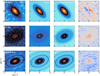 |
Fig. C.3 Continuation of Fig. C.3. |
| In the text | |
Current usage metrics show cumulative count of Article Views (full-text article views including HTML views, PDF and ePub downloads, according to the available data) and Abstracts Views on Vision4Press platform.
Data correspond to usage on the plateform after 2015. The current usage metrics is available 48-96 hours after online publication and is updated daily on week days.
Initial download of the metrics may take a while.