| Issue |
A&A
Volume 670, February 2023
|
|
|---|---|---|
| Article Number | A98 | |
| Number of page(s) | 63 | |
| Section | Interstellar and circumstellar matter | |
| DOI | https://doi.org/10.1051/0004-6361/202244584 | |
| Published online | 14 February 2023 | |
Direct measurements of carbon and sulfur isotope ratios in the Milky Way
1
Max-Planck-Institut für Radioastronomie,
Auf dem Hügel 69,
53121
Bonn, Germany
e-mail: yyan@mpifr-bonn.mpg.de; astrotingyan@gmail.com
2
Astronomy Department, Faculty of Science, King Abdulaziz University,
PO Box 80203,
Jeddah
21589, Saudi Arabia
3
Xinjiang Astronomical Observatory, Chinese Academy of Sciences,
830011
Urumqi, PR China
4
Centre for Astrophysics Research, Department of Physics, Astronomy and Mathematics, University of Hertfordshire,
Hatfield
AL10 9AB, UK
5
Center for Astrophysics, Guangzhou University,
510006
Guangzhou, PR China
6
Ural Federal University,
19 Mira Street,
620002
Ekaterinburg, Russia
7
School of Astronomy and Space Science, Nanjing University,
163 Xianlin Avenue,
Nanjing
210023, PR China
8
Key Laboratory of Modern Astronomy and Astrophysics (Nanjing University), Ministry of Education,
Nanjing
210023, PR China
9
Shanghai Astronomical Observatory,
Shanghai
200030, PR China
Received:
22
July
2022
Accepted:
6
December
2022
Context. Isotope abundance ratios provide a powerful tool for tracing stellar nucleosynthesis, evaluating the composition of stellar ejecta, and constraining the chemical evolution of the Milky Way.
Aims. We aim to measure the 12C/13C, 32S/34S, 32S/33S, 32S/36S, 34S/33S, 34S/36S, and 33S/36S isotope ratios across the Milky Way.
Methods. With the IRAM 30 meter telescope, we performed observations of the J = 2−1 transitions of CS, C33S, C34S, C36S, 13CS, 13C33S, and 13C34S as well as the J = 3−2 transitions of C33S, C34S, C36S, and 13CS toward a large sample of 110 high-mass star-forming regions.
Results. We measured the 12C/13C, 32S/34S, 32S/33S, 32S/36S, 34S/33S, 34S/36S, and 33S/36S abundance ratios with rare isotopologs of CS, thus avoiding significant saturation effects. With accurate distances obtained from parallax data, we confirm previously identified 12C/13C and 32S/34S gradients as a function of galactocentric distance. In the central molecular zone, 12C/13C ratios are higher than suggested by a linear fit to the disk values as a function of galactocentric radius. While 32S/34S ratios near the Galactic center and in the inner disk are similar, this is not the case for 12C/13C, when comparing central values with those near galactocentric radii of 5 kpc. As was already known, there is no 34S/33S gradient but the average ratio of 4.35 ± 0.44 derived from the J = 2−1 transition lines of C34S and C33S is well below previously reported values. A comparison between solar and local interstellar 32S/34S and 34S/33S ratios suggests that the Solar System may have been formed from gas with a particularly high 34S abundance. For the first time, we report positive gradients of 32S/33S, 34S/36S, 33S/36S, and 32S/36S in our Galaxy. The predicted 12C/13C ratios from the latest Galactic chemical-evolution models are in good agreement with our results. While 32S/34S and 32S/36S ratios show larger differences at larger galactocentric distances, 32S/33S ratios show an offset across the entire inner 12 kpc of the Milky Way.
Key words: nuclear reactions, nucleosynthesis, abundances / Galaxy: evolution / Galaxy: formation / ISM: abundances / HII regions / ISM: molecules
© The Authors 2023
 Open Access article, published by EDP Sciences, under the terms of the Creative Commons Attribution License (https://creativecommons.org/licenses/by/4.0), which permits unrestricted use, distribution, and reproduction in any medium, provided the original work is properly cited.
This article is published in open access under the Subscribe to Open model.
Open Access funding provided by Max Planck Society.
1 Introduction
Isotope abundance ratios provide a powerful tool for tracing stellar nucleosynthesis, evaluating the composition of stellar ejecta, and constraining the chemical evolution of the Milky Way (Wilson & Rood 1994). In particular, the 12C/13C ratio is one of the most useful tracers of the relative degree of primary to secondary processing. 12C is a predominantly primary nucleus formed by He burning in massive stars on short timescales (e.g., Timmes et al. 1995). 13C is produced on a longer timescale via CNO processing of 12C seeds from earlier stellar generations during the red giant phase in low- and intermediate-mass stars or novae (e.g., Henkel et al. 1994; Meyer 1994; Wilson & Rood 1994). 12C/13C ratios are expected to be low in the central molecular zone (CMZ) and high in the Galactic outskirts, because the Galaxy formed from the inside out (e.g., Chiappini et al. 2001; Pilkington et al. 2012).
Observations indeed indicate a gradient of 12C/13C ratios across the Galaxy. Wilson et al. (1976) and Whiteoak & Gardner (1979) measured the JKa,Kc = 11,0−11,1 lines of  and
and  near 5 GHz toward 11 and 24 Galactic continuum sources, respectively. While ignoring effects of photon trapping, the results suggested that the 12C/13C ratios may vary with galactocentric distance (RGC). With the additional measurement of the JKa,Kc = 21,1−21,2 line of H2CO at 14.5 GHz, Henkel et al. (1980, 1982, 1983, 1985) also reported a gradient after correcting for effects of optical depth and photon trapping. Langer & Penzias (1990) used the optically thin lines of C18O and 13C18O to trace the carbon isotope ratios. They also found a systematic 12C/13C gradient across the Galaxy, ranging from about 20−25 near the Galactic center, to 30−50 in the inner Galactic disk, to ∼70 in the local interstellar medium (ISM). Wouterloot & Brand (1996), complementing these investigations by also including the far outer Galaxy, encountered ratios in excess of 100 and demonstrated that the gradient found in the inner Galaxy continues farther out. Milam et al. (2005) obtained 12C/>13C = 6.01RGC + 12.28 based on the CN measurements of Savage et al. (2002). Here and elsewhere, RGC denotes the galactocentric distance in units of kiloparsecs (kpc). By combining previously obtained H2CO and C18O results with these CN data, Milam et al. (2005) obtained 12C/13C = 6.21RGC + 18.71.
More recently, Halfen et al. (2017) reported observations of a variety of molecules (e.g., H2CS, CH3CCH, NH2CHO, CH2CHCN, and CH3CH2CN) and their 13C-substituted species toward Sgr B2(N). These authors obtained an average 12C/13C value of 24 ± 7 in the Galactic center region, which is close to results using 12CH/13CH (15.8 ± 2.4, Sgr B2(M)) by Jacob et al. (2020) and the particularly solid 12C34S/13C34S ratio ( , +50 km s−1 Cloud) from Humire et al. (2020) who use a variety of CS isotopologs and rotational transitions. Yan et al. (2019) proposed a linear fit of 12C/13C = (5.08 ± 1.10)RGC + (11.86 ± 6.60) based on a large survey of H2CO. The latter includes data from the center to the outskirts of the Milky Way well beyond the Perseus Arm. However, data from the CMZ are not similar to those thoroughly traced by Humire et al. (2020), not many sources from the innermost Galactic disk could be included in this survey, and also the number of sources beyond the Perseus arm was small, meaning that there is still space for improvement.
While the carbon isotope ratio has drawn much attention in the past, it is not the only isotope ratio that can be studied at radio wavelengths and that has a significant impact on our understanding of the chemical evolution of the Galaxy. The isotope ratios of sulfur are providing complementary information on stellar nucleosynthesis that is not traced by the carbon isotope ratio. Sulfur is special in that it provides a total of four stable isotopes, 32S, 34S, 33S, and 36S. In the Solar System, abundance ratios are 95.02:4.21:0.75:0.021, respectively (Anders & Grevesse 1989). 32S and 34S are synthesized during stages of hydrostatic oxygen-burning preceding a type II supernova event or during stages of explosive oxygen-burning in a supernova of type Ia; 33S is synthesized in explosive oxygen- and neon-burning, which is also related to massive stars; and 36S may be an s-process nucleus. The comprehensive calculations of Woosley & Weaver (1995) indicate that 32S and 33S are primary (in the sense that the stellar yields do not strongly depend on the initial metallicity of the stellar model), while 34S is not a clean primary isotope; its yield decreases with decreasing metallicity. According to Thielemann & Arnett (1985) and Langer (1989), 36S is produced as a purely secondary isotope in massive stars, with a possible (also secondary) contribution from asymptotic giant branch (AGB) stars. Only a small fraction of 36S is destroyed during supernova explosions (Woosley, priv. comm.). Comparing "primary" and "secondary" nuclei, we might therefore expect the presence of weak 32S/34S and 34S/33S gradients and a stronger 32S/36S gradient as a function of galactocentric radius.
There is a strong and widespread molecular species that allows us to measure carbon and sulfur isotope ratios simultaneously, namely carbon monosulfide (CS). CS is unique in that it is a simple diatomic molecule exhibiting strong line emission and possessing eight stable isotopologs, which allows us to determine the above-mentioned carbon and sulfur isotope ratios. Six isotopologs have been detected so far in the ISM (e.g., Chin et al. 1996; Mauersberger et al. 1996; Humire et al. 2020; Yu et al. 2020).
Making use of the CS species, Chin et al. (1996) and Mauersberger et al. (1996) obtained average abundance ratios of 24.4 ± 5.0, 6.3 ± 1.0, and 115 ± 17 for 32S/34S, 34S/33S, and 34S/36S for the ISM, respectively. The latter is approximately half the solar value, but similar to the value found in IRC+10216 (Mauersberger et al. 2004). Recently, Humire et al. (2020) published 32S/34S ratios of  and 17.9 ± 5.0 for the +50 km s−1 cloud and Sgr B2(N) near the Galactic center, respectively. These are only slightly lower than the value of 22 in the Solar System. There is an obvious and confirmed 32S/34S gradient (Chin et al. 1996; Yu et al. 2020) from the inner Galaxy out to a galactocentric distance of 12.0 kpc. Nevertheless, there is a lack of data at small and large galactocentric distances.
We are performing systematic observational studies on isotope ratios in the Milky Way, including 12C/13C (Yan et al. 2019), 14N/15N (Chen et al. 2021),18O/17O (Zhang et al. 2015, 2020a, 2020b; Li et al. 2016), and 32S/34S (Yu et al. 2020). We have thus performed a more systematic study on CS and its iso-topologs toward 110 high-mass star-forming regions (HMSFRs). 12C/13C and 32S/34S ratios can be directly derived from integrated 12C34S/13C34S (hereafter C34S/13C34S) and 13C32S/13C34S (hereafter 13CS/13C34S, see Sect. 3.2) intensities, respectively. Also, 34S/33S and 34S/36S values could be obtained with measurements of C34S, 12C33S (hereafter C33S), and 12C36S (hereafter C36S). Furthermore, 32S/33S and 32S/36S ratios can then be derived with the resulting 34S/33S and 34S/36S values combined with the 32S/34S ratios (see Sects. 3.4–3.7). In Sect. 2, we describe the source selection and observations for our large sample. Section 3 presents our results on 12C/13C, 32S/34S, 34S/33S, 32S/33S, 34S/36S, and 32S/36S ratios. Section 4 discusses potential processes that could contaminate and affect the isotope ratios derived in the previous section and provides a detailed comparison with results from earlier studies. Our main results are summarized in Sect. 5.
2 Source selection and observations
2.1 Sample selection and distance
In 2019, we selected 18 HMSFRs from the Galactic center region to the outer Galaxy beyond the Perseus arm. To enlarge this sample, we chose 92 sources from the Bar and Spiral Structure Legacy (BeSSeL) Survey1 in 2020. These 92 targets were recently released by the BeSSeL project (Reid et al. 2019) and not observed by Yu et al. (2020). In total, 110 objects in the Galaxy are part of our survey. The coordinates of our sample sources are listed in Table A.1. Determining trigonometric parallaxes is a very direct and accurate method to measure the distance of sources from the Sun (Reid et al. 2009, 2014, Reid et al. 2019). Over the past decade, mainly thanks to the BeSSeL project, the trigonometric parallaxes of approximately 200 HMSFRs have been determined across the Milky Way through dedicated high-resolution observations of molecular maser lines. Therefore, this is a good opportunity to investigate carbon and sulfur isotope ratios with well-determined distances across the Galaxy. The galactocentric distance (RGC) can be obtained with the heliocentric distance d from the trigonometric parallax data base of the BeSSeL project using
 (1)
(1)
(Roman-Duval et al. 2009). R0 = 8.178 ± 0.013stat. ± 0.022sys. kpc (GRAVITY Collaboration 2019) describes the distance from the Sun to the Galactic center, l is the Galactic longitude of the source, and d is the distance either directly derived from the trigonometric parallax data based on the BeSSeL project or a kinematic distance in cases where no such distance is yet available. Because the uncertainty in R0 is very small, it will be neglected in the following analysis. For 12 of our targets without trigonometric parallax data, we estimated their kinematic distances from the Revised Kinematic Distance calculator2 (Reid et al. 2014). The resulting distances indicate that 6 of these 12 sources are located in the CMZ, namely SgrC, the +20 km s−1 cloud, the +50 km s−1 cloud, G0.25, G1.28+0.07, and SgrD. Four targets belong to the inner Galactic disk, namely PointC1, CloudD, Clump2, and PointD1. Two sources, W89-380 and WB89-391, are in the outer regions beyond the Perseus arm. The heliocentric distances (d) and the galactocentric distances (RGC) for our sample are listed in Cols. 6 and 7 of Table A.1.
2.2 Observations
We observed the J = 2−1 transitions of CS, C33S, C34S, C36S, 13CS, 13C33S, and 13C34S as well as the J = 3−2 transitions of C33S, C34S, C36S, and 13CS toward 110 HMSFRs with the IRAM 30 meter telescope3 in 2019 June, July, and October under project 045-19 (PI, Christian Henkel) as well as in 2020 August within project 022-20 (PI, Hongzhi Yu). The on + off source integration times for our sources range from 4.0 min to 10.8 h. These values are given in Table A.3. The EMIR receiver with two bands, E090 and E150, was used to cover a bandwidth of ∼16 GHz (from 90.8 to 98.2 GHz and 138.4 to 146.0 GHz) simultaneously in dual polarisation. We used the wide-mode FTS backend with a resolution of 195 kHz, corresponding to ∼0.6 km s−1 and ∼0.4km s−1 at 96 GHz and 145 GHz, respectively. The observations were performed in total-power position-switching mode and the off position was set at 30' in azimuth. Pointing was checked every 2 h using nearby quasars. Focus calibrations were done at the beginning of the observations and during sunset and sunrise toward strong quasars. The main beam brightness temperature, TMB, was obtained from the antenna temperature  via the relation
  (Feff: forward hemisphere efficiency; Beff: main beam efficiency) with corresponding telescope efficiencies4: Feff/Beff are 0.95/0.81 and 0.93/0.73 in the frequency ranges of 90.8–98.2 GHz and 138.4–146.0 GHz, respectively. The system temperatures were 100–160 K and 170–300 K on a
  scale for the E090 and E150 band observations. The half power beam width (HPBW) for each transition was calculated as HPBW(") = 2460/v(GHz). Rest frequencies, excitations of the upper levels above the ground state, Einstein coefficients for spontaneous emission, and respective beam sizes are listed in Table 1.
Observed spectral line parameters.
2.3 Data reduction
We used the GILDAS/CLASS5 package to analyze the spectral line data. The spectra of the J = 2−1 transitions of CS, C33S, C34S, C36S, 13CS,13C33S, and 13C34S as well as the J = 3−2 transitions of C33S, C34S, C36S, and 13CS toward one of our targets, DR21, are shown in Fig. 1, after subtracting first-order polynomial baselines and applying Hanning smoothing. The spectra of all 110 targets, also after first-order polynomial-baseline removal and Hanning smoothing, are presented in Fig. B.1.
Among our sample of 110 targets, we detected the J = 2−1 line of CS toward 106 sources, which yields a detection rate of 96%. The J = 2−1 transitions of C34S, 13CS, C33S, and 13C34S were successfully detected in 90, 82, 46, and 17 of our sources with signal-to-noise ratios (S/N) of greater than 3, respectively. The J = 3−2 lines of C34S, 13CS, and C33S were detected in 87, 71, and 42 objects with S/Ns of ≥3.0. Line parameters from Gaussian fitting are listed in Table A.3. Relevant for the evaluation of isotope ratios is the fact that for 17 sources with 19 velocity components, the S/Ns of the J = 2−1 transition of 13C34S are greater than 3, which allows us to determine the 12C/13C and 32S/34S ratios directly with the J = 2−1 lines of C34S, 13CS, and 13C34S. Toward 82 targets with 90 radial velocity components, the J = 2−1 transitions of C34S and 13CS were both detected with S/Ns of ≥3.0. The J = 3−2 lines of C34S and 13CS were both found in 71 objects with 73 radial velocity components and S/Ns of ≥3.0. Furthermore, the J = 2−1 and J = 3−2 transitions of C34S and C33S were detected with S/Ns of ≥3.0 toward 46 and 42 sources, respectively.
The C36S J = 2−1 line was successfully detected with S/Ns of ≥3.0 toward three targets, namely W3OH, the +50 km s−1 cloud near the Galactic center, and DR21. As C36S and 13C33S are the least abundant among the CS isotopologs, tentative detection with S/Ns of ∼2.0 are also presented here but not included in further analyses. In another five objects, the C36S J = 2−1 line was tentatively detected. For the C36S J = 3−2 transitions, we report one detection with an S/N larger than 3.0 toward Orion-KL and five tentative detections. The J = 2−1 lines of 13C33S were tentatively detected toward three sources, namely Orion-KL, W51-IRS2, and DR21. Integration times and 1σ noise levels of the observed transitions are listed in Cols. 3 and 4 of Table A.3 for each target.
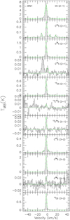 |
Fig. 1 Line profiles of the J = 2−1 transitions of CS, C33S, C34S, C36S, 13CS, 13C33S, and 13C34S as well as the J = 3−2 transitions of C33S, C34S, C36S, and 13CS toward one typical target (DR21) of our large sample of 110 sources, after subtracting first-order polynomial baselines. The main beam brightness temperature scales are presented on the left hand side of the profiles. The spectra of all 110 objects in our sample are shown in Fig. B.1. |
3 Results
In the following, we first estimate the optical depths of the various lines to avoid problems with line saturation that might affect our results. We then present the carbon and sulfur isotope ratios derived from different detected CS isotopologs.
3.1 Optical depth
The main isotopolog, CS, is usually optically thick in massive star-forming regions (e.g. Linke & Goldsmith 1980; Yu et al. 2020). Therefore, the 12C/13C and 32S/34S ratios cannot be determined from the line intensity ratios of I(CS)/I(13CS) and I(CS)/I(C34S). However, assuming that the J = 2−1 transitions of CS, C34S, and 13CS share the same beam filling factor and excitation temperature, we can estimate the maximum optical depth of the 13CS J = 2−1 line from:
 (2)
(2)
where Tmb is the peak main beam brightness temperature derived from the best Gaussian-fitting result and listed in Col. 8 of Table A.3. In this case, the 12C/13C ratios can be derived from the integrated line intensities of C34S and 13C34S with the assumption of τ(C34S) < 1.0, which then also implies τ(13C34S) < 1.0 (see details in Sect. 3.2). Multiplying τ(13CS) by RC = 12C/13C, we can get the peak opacity τ(CS) = τ(13CS)RC. The maximum optical depth of C34S can be obtained from:
 (3)
(3)
where Tmb is the peak main beam brightness temperature derived from the best Gaussian-fitting result and listed in Col. 8 of Table A.3. As shown in Table 2, the peak optical depths of the J = 2−1 lines of CS, C34S, and 13CS for our 17 targets with detections of 13C34S range from 1.29 to 8.79, 0.12 to 0.55, and 0.05 to 0.34, respectively. Therefore, C34S and 13CS in these 17 objects are optically thin, even though they belong, on average, to the more opaque ones, being successfully detected in 13C34S (see below). Nevertheless, the corrections for optical depth are applied to C34S and 13CS with factors of f1 and f2, respectively.
 (4)
(4)
 (5)
(5)
are listed in Cols. 7 and 8 of Table 2, respectively.
For those 82 sources with detections of J = 2−1 CS, C34S, and 13CS, the optical depths were calculated based on the 12C/13C gradient that we derived from our C34S and 13C34S measurements (for details, see Sect. 3.2). In Table A.2, the peak opacities of the J = 2−1 lines of CS, C34S, and 13CS for these 82 targets range from 0.34 to 14.48, 0.02 to 0.74, and 0.01 to 0.39, respectively. The CS J = 2−1 lines are optically thick with τ(CS) > 1.0 in most sources (89%) of our sample, while they tend to be optically thin in seven objects, namely Point C1 (τ(CS) ≤ 0.59), Sgr C (τ(CS) ≤ 0.54), Cloud D (τ(CS) ≤ 0.64), G1.28+0.07 (τ(CS) ≤ 0.82), Sgr D (τ(CS) ≤ 0.45), and Point D1 (τ(CS) ≤ 0.34). In contrast, the transitions from rare isotopologs, the C34S and 13CS J = 2−1 lines in our sample, are all optically thin, as their maximum optical depths are less than 0.8 and 0.4, respectively. In the following, we are therefore motivated to consider all CS isotopologs as optically thin, except CS itself. This allows us to use ratios of integrated intensity of all the rare CS isotopologs – but not CS itself – to derive the carbon and sulfur isotope ratios we intend to study. Small corrections accounting for the optical depths are applied to the C34S and 13CS J = 2−1 lines with factors of f1 and f2, respectively, and are listed in Cols. 7 and 8 of Table A.2. The optical depths of the J = 3−2 transitions cannot be estimated, as the CS J = 3−2 line was not covered by our observations because of bandwidth limitations. However, the 32S/34S ratios for a given source obtained through the double isotope method from the J = 2−1 and J = 3−2 transitions are in good agreement, indicating that the C34S and 13CS J = 3−2 lines in our sample are also optically thin (see details in Sect. 3.3).
The RADEX non Local Thermodynamic Equilibrium (LTE) model (van der Tak et al. 2007) was used to calculate the variation of excitation temperature, Tex, with optical depth. Frequencies, energy levels, and Einstein A coefficients for spontaneous emission were taken from the Cologne Database for Molecular Spectroscopy (CDMS; Müller et al. 2005; Endres et al. 2016). Recent collision rates for CS with para- and ortho-H2 (Denis-Alpizar et al. 2018) were used. Figure 2 shows the excitation temperatures and opacities of C34S J = 2−1 for a kinetic temperature of 30 Κ and a molecular hydrogen density of 105 cm−3. Variations of Tex within about 2 Κ for our sample targets with optical depths of 0.02 ≤ τ(C34S) ≤ 0.74 can barely affect our results.
Isotope ratios derived with the J = 2−1 transitions of C34S, 13CS, and 13C34S.
3.2 12C/13C and 32S/34S ratios derived directly from 13C34S
3.2.1 12C/13C ratios
The 12C/13C ratios derived from the integrated intensity ratios of C34S and 13C34S with corrections of optical depth are listed in Table 2. Figure 3 shows our results as filled black circles. A gradient of 12C/13C is obtained with an unweighted least-squares fit:
 (6)
(6)
The correlation coefficient is 0.82. Around the CMZ toward the +50 km s−1 cloud and SgrB2, four velocity components of C34S and 13C34S were detected and then an average 12C/13C value of 27 ± 3 is derived. The uncertainties given here and below are standard deviations of the mean. Eleven objects within a range of 3.50 kpc < RGC < 6.50 kpc in the inner Galactic disk lead to an average 12C/13C value of 41 ± 9. In the Local arm near the Sun, the 13C34S lines were detected toward two sources, Orion-KL and DR21. These provide an average 12C/13C value of 66 ± 10, which is lower than the Solar System ratio. The other two targets beyond the solar neighborhood belong to the Perseus arm and show a slightly higher value of 74 ± 8.
For sources with detections of C34S and nondetections of 13C34S, 3σ lower limits of the 12C/13C ratio have been derived and are shown as open black circles in Fig. 3. All these lower limits are below the 12C/13C gradient we describe above.
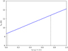 |
Fig. 2 Excitation temperature, Tex, as a function of optical depth for the J = 2−1 transition of C34S. The gray dashed lines indicate the range of opacities for our sample sources. |
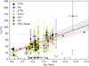 |
Fig. 3 12C/13C isotope ratios from C34S/13C34S, CN/13CN, C18O/13C18O, |

3.2.2 32S/34S ratios
The 32S/34S ratios directly derived from the integrated intensity ratios of 13CS/13C34S from the J = 2−1 lines with corrections of optical depth are listed in Table 2 and are plotted as a function of galactocentric distance in Fig. 4. With an unweighted least-squares fit, a gradient with a correlation coefficient of 0.47 can be obtained:
 (7)
(7)
An average 32S/34S ratio of 19 ± 2 is obtained in the CMZ, which is based on the measurements from two sources, namely the +50 km s−1 cloud next to the Galactic center and Sgr B2. In the inner Galactic disk at a range of 3.50 kpc < RGC <6.50 kpc, 13C34S was detected toward 11 objects, leading to an average 32S/34S value of 18 ± 4. For sources in the Local and the Perseus arm beyond the Sun, the 32S/34S ratios are 24 ± 4 and 28 ± 3, respectively. This reveals a gradient from the inner Galactic disk to the outer Galaxy, but none from the CMZ to the inner disk.
For sources with detections of 13CS and nondetections of 13C34S, we determined 3σ lower limits to the 32S/34S ratio, which are shown as open black circles in Fig. 4. All these lower limits are below the 32S/34S gradient we describe above.
3.3 32S/34S ratios obtained through the double isotope method
The 32S/34S values can also be derived from measurements of C34S and 13CS using the carbon gradient obtained from our 13C34S measurements above by applying the following equation:
 (8)
(8)
where RC is the 12C/13C ratio derived from Eq. (6). The uncertainty on this latter is also included in our error budget. The 32S/34S ratios in the J = 2−1 transitions were calculated with corrections of optical depth for 83 targets with 90 radial velocity components, in which the C34S and 13CS J = 2−1 lines were both detected, and are listed in Col. 7 of Table A.2. An unweighted least-squares fit to these values yields
 (9)
(9)
with a correlation coefficient of 0.54. The C34S and 13CS J = 3−2 lines were both detected in 71 objects with 73 radial velocity components. The 32S/34S ratios derived with Eq. (8) from the J = 3−2 transition are shown in Col. 8 of Table A.2. An unweighted least-squares fit to the J = 3−2 transition yields
 (10)
(10)
which is within the errors, and is consistent with the trend obtained from the J = 2−1 transition (Eq. (9)). However, we note that we do not have CS J = 3−2 data, and therefore no opacity corrections could be applied to our C34S J = 3−2 spectra (see also Sect. 3.4).
3.4 34S/33S ratios
The 34S/33S ratios can be determined directly from the intensity ratios of C34S/C33S. The 34S/33S ratios from the J = 2−1 lines were then corrected for optical depths derived in Sect. 3.1. However, both the J = 2−1 and J = 3−2 transitions of C33S are split by hyperfine structure (HFS) interactions (Bogey et al. 1981), which may affect the deduced values of 34S/33S.
The C33S J = 2−1 line consists of eight hyperfine components distributed over about 9.0 MHz (Müller et al. 2005; Endres et al. 2016), which corresponds to a velocity range of about 28 km s−1. Following the method introduced in Appendix D in Gong et al. (2021), and assuming that the intrinsic width of each HFS line is 1 km s−1, the J = 2−1 line profile can be reproduced by four components (see Fig. 5, upper left panel). In this case, the main component (Imain) consists of four HFS lines (F = 7/2−5/2, F = 5/2−3/2, F = 1/2−1/2, F = 3/2−5/2), which account for 70% of the total intensity. Among the 46 sources with detections of the C33S J = 2−1 line, all of the four components were detected in 10 targets. Toward 16 objects, only the three components with the lowest velocities were detected, accounting for 98% of the total intensity. For the remaining 20 sources, only the main component was detected. Based on the above assumptions, 30% of the total intensity would be missed. The situation is different when the main component becomes broader. If the line width of the main component is larger than 10 km s−1, 87% of the total intensity is covered by the main spectral feature. When the line width of the main component is larger than 19.0 km s−1, then almost all HFS lines are included. In Fig. 6, we show the dependence of the HFS factor for the J = 2−1 line, f21HFS, on the line width of the main component. Depending on the specific condition of each target, we derived f21HFS for each source. The values are listed in Table 3.
The C33S J = 3−2 line consists of nine hyperfine components covering about 8.0 MHz (Müller et al. 2005; Endres et al. 2016), corresponding to a velocity range of about 16 km s−1. Assuming that the intrinsic width of each HFS line is 1 km s−1, the J = 3−2 line profile can be characterized by three components (see also Fig. 5). All these three components are detected in only two sources, Orion-KL and DR21. The main component consists of four HFS lines (F = 5/2−3/2, F = 3/2−1/2, F = 7/2−5/2, F = 9/2−7/2), which account for 86% of the total intensity. When the line width becomes larger than 9.2 km s−1, almost all of the HFS lines overlap. The HFS factors (f32HFS) of the J = 3−2 transition obtained individually for each source are listed in Table 3.
We calculated the 34S/33S intensity ratios and present them in Table 3. Applying corrections accounting for the effect of hyperfme splitting, the 34S/33S ratios are derived and are also listed in Table 3. The 34S/33S values obtained from the J = 2−1 transitions are always higher than the ones derived from the J = 3−2 lines toward the same source, with the exception of G097.53+03.18. This difference could be caused by the lack of corrections of optical depth in the J = 3−2 transition. The average values of 34S/33S toward our sample are 4.35 + 0.44 and 3.49 + 0.26 in the J = 2−1 and J = 3−2 transitions, respectively. The 34S/33S ratios were found to be independent of galactocentric distance (Fig. 7).
After applying the opacity correction of the J = 2−1 transition to the J = 3−2 line in the same source, 34S/33S ratios in the J = 3−2 transition are higher than the 34S/33S values in the J = 2−1 transition in seven targets, suggesting that the C34S J = 3−2 lines in these seven sources are less opaque than the C34S J = 2−1 lines. The seven targets are the +20 km s−1 cloud, G023.43-00.18, G028.39+00.08, G028.83-00.25, G073.65+00.19, G097.53+03.18, and G109.87+02.11. A comparison of the corrected 34S/33S ratios in these two transitions is shown in Fig. 8. On the other hand, toward the other 32 objects of the whole sample of 39 sources with detections in these two transitions, the 34S/33S ratios in the J = 3−2 transition are still lower than the 34S/33S values in the J = 2−1 transitions. This suggests that the C34S J = 3−2 lines may be more opaque than the C34S J = 2−1 lines. The ratios of 34S/33S values without corrections of opacity in the J = 3−2 transition and the corrected 34S/33S values from the J = 2−1 lines in 31 targets of these 32 sources are within the range of 1.02 to 1.71, which suggest that the optical depths of C34S in the J = 3−2 transition in these objects range from 0.05 to 1.20 based on Eq. (4). The maximum optical depth of the C34S J = 3−2 line toward the additional source, G024.85+00.08, which has not considered until now, is estimated to be 2.6.
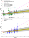 |
Fig. 4 32S/34S isotope ratios as functions of the distance from the Galactic center. The symbol ⊙ indicates the 32S/34S isotope ratio in the Solar System. In the upper panel, the 32S/34S ratios directly derived from 13CS/13C34S in the J = 2−1 transition and obtained from the double isotope method in the J = 2−1 transition with corrections for optical depth are plotted as black and green dots, respectively. The 32S/34S ratios without corrections of opacity in the J = 3−2 transition are plotted as light blue dots. The 3σ lower limits of 32S/34S ratios obtained from non-detections of 13C34S in the current work are shown as open black circles. The 32S/34S ratios in Yu et al. (2020) derived from the double isotope method in the J = 2−1 transitions are shown as blue dots in the lower panel. The 32S/34S values in the CMZ obtained from 13CS/13C34S in Humire et al. (2020) are plotted as red stars in both panels. The resulting first-order polynomial fits to 32S/34S ratios with the direct method and the double isotope method from the J = 2−1 transition in this work are plotted as black and red solid lines in the two panels, respectively, with the gray and yellow shaded areas showing the 1 σ intervals of the fits. The magenta and cyan dashed-dotted lines show the 32S/34S gradients from Chin et al. (1996) and Yu et al. (2020). The red crosses visualize the results from the GCE model of Kobayashi et al. (2011, 2020, see also Sect. 4.9). |
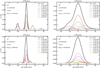 |
Fig. 5 Synthetic C33S (2−-1) and C33S (3−2) spectra for two intrinsic line widths, 1.0 km s−1 (left panels) and 4.0 km s−1 (right panels). |
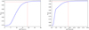 |
Fig. 6 Blue lines are curves showing the theoretical dependencies of the HFS factors, f21HFS (left) and f32HFS (right), on the line width of the C33S main component for sources in which only the main component was detected. The red dotted vertical and horizontal lines indicate the values of the minimal line widths where the factors are reaching almost 1.0, 19.0 km s−1 for the J = 2−1 transition (f21HFS ∼ 0.99) and 9.2 km s−1 for the J = 3−2 transition (f32HFS ∼ 0.99). |
3.5 32S/33S ratios
The 32S/33S values can also be derived from the 34S/33S ratios in Sect. 3.4 using the 32S/34S ratios – which we directly obtained from 13CS/13C34S and present in Sect. 3.2.2 – by applying the following equation:
 (11)
(11)
For sources where we did not detect 13C34S, the 32S/34S ratios derived from the double isotope method in Sect. 3.3 are used. Their uncertainty is also included in our error budget. The resulting 32S/33S ratios are listed in Table 4. As in the case of the 34S/33S ratios, the32S/33S values obtained from the J = 2−1 transitions with corrections for optical depth are slightly larger than the ones from the J = 3−2 transitions without opacity corrections toward the same source.
In the CMZ, 32S/33S J = 2−1 ratios toward four targets, namely the +20 km s−1 cloud, the +50 km s−1 cloud, Sgr B2, and Sgr D, lead to an average value of 70 ± 16. In the inner Galaxy, in a galactocentric distance range of 2.0 kpc ≤ RGC ≤ 6.0 kpc, an average 32S/33S ratio of 82 ± 19 was derived from values in 20 sources. Near the solar neighborhood, in a galactocentric distance range of 7.5 kpc ≤ RGC ≤ 8.5 kpc, 32S/33S ratios were obtained toward four objects, Orion-KL, G071.31+00.82, DR21, and G109.87+02.11, resulting in an average value of 88 ± 21. For the outer Galaxy, beyond the local arm, we were able to deduce an average 32S/33S ratio of 105 ± 19 from 32S/33S values in four sources. All these average values provide us with an indication of the existence of a 32S/33S gradient in the Galaxy. An unweighted least-squares fit to the J = 2−1 transition data from 46 sources yields
 (12)
(12)
In the J = 3−2 transition with data from 42 targets, an unweighted least-squares fit can be obtained with
 (13)
(13)
The 32S/33S gradients derived from these two transitions have similar slopes but obviously different intercepts. The lower intercept in the J = 3−2 transition could be due to the fact that we could not correct the values for optical-depth effects. If this difference is caused only by the opacity, then an average optical depth in the C34S J = 3−2 transition of about 0.4 can be derived with Eq. (4).
Corrected 34S/33S isotope ratios.
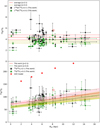 |
Fig. 7 34S/33S and 32S/33S isotope ratios (for the latter, see Eqs. (12) and (13)) plotted as functions of the distance from the Galactic center. Top: 34S/33S ratios derived from C34S/C33S in the J = 2−1 and J = 3−2 transitions plotted as black and green dots, respectively. The red solid and the two dashed lines show the average value and its standard deviation, 4.35 ± 0.44, of 34S/33S with corrections of optical depth toward our sample in the J = 2−1 transition. The yellow solid and the two dashed lines show the average value and its standard deviation, 3.49 ± 0.26, of 34S/33S toward our sample in the J = 3−2 transition. The red symbol ⊙ indicates the 34S/33S isotope ratio in the Solar System. Bottom: Black and green dots show the 32S/33S ratios in the J = 2−1 and J = 3−2 transitions, respectively. The red symbol ⊙ indicates the 32S/33S value in the Solar System. The resulting first-order polynomial fits to the 32S/33S ratios in the J = 2−1 and J = 3−2 transitions in this work are plotted as red and green solid lines, respectively, with the pink and yellow shaded area showing the 1 σ standard deviations. The red crosses are the results from the GCE model of Kobayashi et al. (2011, 2020, see also Sect. 4.9). |
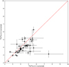 |
Fig. 8 Comparison of 34S/33S ratios between the J = 2−1 and 3−2 data. The J = 2−1 ratios are opacity corrected, while the same correction factors were also applied to the J = 3−2 data. The red solid line indicates that the 34S/33S ratios are equal in these two transitions. |
32S/33S isotope ratios.
3.6 34S/36S ratios
The detection of C36S in the J = 2−1 and J = 3−2 transitions allows us to also calculate 34S/36S ratios. Around the CMZ, the C36S J = 2−1 line in the +50 km s−1 cloud was detected, resulting in a 34S/36S ratio of 41 ± 4. In the local arm toward DR21 and Orion-KL (Menten et al. 2007; Xu et al. 2013), the C36S J = 2−1 and J = 3−2 transitions were detected, respectively, leading to 34S/36S values of 117 ± 24 and 83 ± 7. This yields an average 34S/36S ratio of 100 ± 16 in the ISM near the Sun. In the Perseus arm beyond the Solar System (Xu et al. 2006), we detected the C36S J = 2−1 line toward W3OH and obtained a 34S/36S value of 140 ± 16. These results reveal the possibility of the existence of a 34S/36S gradient from the Galactic center region to the outer Galaxy. Five tentative detections in the C36S J = 2−1 line and also five tentative detections in the J = 3−2 line provide additional 34S/36S ratios but with large uncertainties. All of the 34S/36S values are listed in Table 5 and are plotted as a function of the distance to the Galactic center in Fig. 9.
Isotope ratios of 34S/36S and 32S/36S.
3.7 32S/36S ratios
As in the case of the 32S/33S ratios, the 32S/36S values could also be obtained from the resulting 34S/36S ratios in Sect. 3.6 and the 32S/34S ratios in Sect. 3.2.2 using the following equation:
 (14)
(14)
The uncertainties of both isotope ratios in the product on the right-hand side of the equation are included in our error budget. The resulting 32S/36S ratios are listed in Table 5. In the CMZ, a 32S/36S ratio of 884 ± 104 is obtained toward the +50 km s−1 cloud.32S/36S values of 1765 ± 414 and 3223 ± 742 are derived toward Orion-KL and DR21, leading to an average 32S/36S value of 2494 ± 578 in the local regions near the Solar System. In the Perseus arm beyond the solar neighborhood toward W3OH, we obtain the highest 32S/36S value, 4181 ± 531. All these results indicate that there could be a positive 32S/36S gradient from the Galactic center region to the outer Galaxy. Figure 9 shows the 32S/36S ratios plotted as a function of the distance to the Galactic center.
4 Discussion
With the measurements of optically thin lines of the rare CS isotopologs, C34S, 13CS, C33S, 13C34S, and C36S, we derived 12C/13C, 32S/34S, 34S/33S, 32S/33S, 34S/36S, and 32S/36S isotope ratios. Combined with accurate galactocentric distances, we established a 32S/33S gradient for the first time and confirmed the existing gradients of 12C/13C and 32S/34S, as well as uniform 34S/33S ratios across the Milky Way, which are lower than previously reported. Furthermore, we may have detected 34S/36S and 32S/36S gradients for the first time. In Sect. 4.1, we compare the 12C/13C gradient obtained in this work with previous published ones derived from a variety of molecular species. A comparison between the 32S/34S gradients we obtained and previously published ones is presented in Sect. 4.2. The condition of LTE for C33S with its HFS line ratios is discussed in Sect. 4.3. We then also compare our results on 34S/33S ratios with previously published values and discuss the 32S/33S gradient. In Sect. 4.4, we evaluate whether or not 34S/36S, 33S/36S, and 32S/36S ratios may show gradients with galactocentric distance. Observational bias due to distance effects, beam size effects, and chemical fractionation are discussed. A comparison of several isotopes with respect to primary or secondary synthesis is provided in Sect. 4.8. Results from a Galactic chemical evolution (GCE) model, trying to simulate the observational data, are presented in Sect. 4.9.
4.1 Comparisons of 12C/13C ratios determined with different species
12C/13C ratios have been well studied in the CMZ where the value is about 20−25 (e.g., Henkel et al. 1983; Güsten et al. 1985; Langer & Penzias 1990; Milam et al. 2005; Riquelme et al. 2010; Belloche et al. 2013; Halfen et al. 2017; Humire et al. 2020),
similar to the results that we obtained from C34S in the current work. In the inner Galaxy, the 12C/13C ratios are higher than the values in the CMZ, which were ∼50 as derived from  in Henkel et al. (1985) and 41 ± 9 from C34S/13C34S in this work. As can be inferred from Fig. 3,12C/13C ratios at 3.0 kpc ≤ RGC ≤ 4.0 kpc might be as low as in the CMZ, but this is so far tentative and uncertain, as we only have one detection (G024.78+00.08) in this region and data from other groups referring to this small galactocentric interval are also relatively few. In the local regions near the Solar System, an average 12C/13C ratio of 66 ± 10 was obtained from C34S/13C34S in this work, which is consistent with 12C/13C values derived from other molecular species and their 13C isotopes, that are 75 ± 9 from C18O (Keene et al. 1998), 60 ± 19 from CN (Milam et al. 2005), 74 ± 8 from CH+ (Ritchey et al. 2011), and 53 ± 16 from H2CO (Yan et al. 2019). All these 12C/13C values for the solar neighborhood are well below the value for the Sun (89, Anders & Grevesse 1989; Meibom et al. 2007). This indicates that 13C has been enriched in the local ISM during the last 4.6 billion years following the formation of the Solar System. Beyond the Sun, at a galactocentric distance of about 10 kpc, our results from C34S/13C34S show a slightly higher value of 67 ± 8, which is similar to 12C/13C ratios from CN (66 ± 20), C18O (69 ± 10), and H2CO (64 ± 10). These values are still below the value for the Sun. In the far outer Galaxy at 13.8 kpc toward WB89 437, Wouterloot & Brand (1996) found a 3σ lower limit of 201 ± 15 from C18O/13C18O. This suggests that the 12C/13C gradient extends well beyond the solar neighborhood to the outer Galaxy. Additional sources with large galactocentric distances have to be measured to further improve the statistical significance of this result.
Previously published 12C/13C ratios derived from CN (Savage et al. 2002; Milam et al. 2005), C18O (Langer & Penzias 1990; Wouterloot & Brand 1996; Keene et al. 1998), H2CO (Henkel et al. 1980, 1982, 1983, 1985; Yan et al. 2019), CH+ (Ritchey et al. 2011), and CH (Jacob et al. 2020) are shown in Fig. 3, but with respect to the new distance values (see details in Sect. 2.1). In Fig. 10, the12C/13C values from different molecular species are projected onto the Galactic plane. This also visualizes the gradient from the Galactic center to the Galactic outer regions beyond the Solar System. In Table 6, the fitting results for the old and new distances are presented. The comparison shows that the adoption of the new distances has indeed an effect on the fitting results, such as for the 12CN/13CN gradient. In Savage et al. (2002) and Milam et al. (2005), the slope and intercept become (6.75 ± 1.44) and (5.77 ± 11.29) from (6.01 ± 1.19) and (12.28 ± 9.33), respectively. The fitting for  from Henkel et al. (1980, 1982, 1983, 1985) and Yan et al. (2019) becomes (5.43 ± 1.04) and (13.87 ± 6.38) from (5.08 ± 1.10) and (11.86 ± 6.60), respectively. The Galactic 12C/13C gradients derived based on measurements of CN, C18O, and H2CO are in agreement with our results from C34S and therefore indicate that chemical fractionation has little effect on the 12C/13C ratios. It is noteworthy that all these fits show a significant discrepancy with observations from the Galactic center. Indeed, they suggest values of 5–17 at RGC = 0, substantially below observed values of 20−25 (see also Tables 6, 7). While the values in the CMZ are clearly lower than in the inner Galactic disk (with the potential exception at galactocentric distances of 2.0−4.0 kpc), they are larger than suggested by a linear fit encompassing the entire inner 12.0 kpc of the Galaxy.
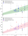 |
Fig. 9 J = 2−1 (opacity corrected) and J = 32 (no opacity corrections) 34S/36S and 32S/36S isotope ratios (see Eqs. (18) and (19)) plotted as functions of the distance from the Galactic center. Top: Filled black circles and filled black triangle present the 34S/36S ratios in the J = 2−1 and J = 3−2 transitions derived from C34S/C36S in this work with detections of C36S, respectively. The open gray circles and open gray triangles present the 34S/36S ratios in the J = 2−1 and J = 3−2 transitions derived from C34S/C36S in this work with tentative detections of C36S, respectively. The blue diamonds show the 34S/36S ratios in Mauersberger et al. (1996). The red symbol ⊙ indicates the 34S/36S isotope ratio in the Solar System. The resulting first-order polynomial fit to the 34S/36S ratios in Mauersberger et al. (1996) and this work, excluding the values from tentative detections, is plotted as a black solid line, with the green shaded area showing the 1 σ interval of the fit. Bottom: 32S/36S ratios obtained from 34S/36S ratios combined with the 32S/34S ratios derived in this work. The filled black circles and filled black triangle present the values in the J = 2−1 and J = 3−2 transitions from this work with detections of C36S, respectively. The open gray circles and open gray triangles present ratios in the J = 2−1 and J = 3−2 transitions from this work with tentative detections of C36S, respectively. The 32S/36S ratios derived with 34S/36S values from Mauersberger et al. (1996) are plotted as blue diamonds. The red symbol ⊙ indicates the 32S/36S isotope ratio in the Solar System. The 32S/36S gradient, excluding tentative detections, is plotted as a black solid line, with the pink shaded area showing the 1 σ interval of the fit. The red crosses visualize results from the GCE model of Kobayashi et al. (2011, 2020, see Sect. 4.9). |
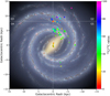 |
Fig. 10 Distribution of 12C/13C ratios from 93 sources in the Milky Way. The background image is the structure of the Milky Way from the artist's impression [Credit: NASA/JPL-Caltech/ESO/R. Hurt]. The 12C/13C isotope ratios with corrections for optical depth from C34S/13C34S in this work are plotted as circles. The triangles, pentagons, stars, squares, and diamonds indicate the 12C/13C ratios derived from CN/13CN (Savage et al. 2002; Milam et al. 2005), C18O/13C18O (Langer & Penzias 1990; Wouterloot & Brand 1996; Keene et al. 1998), |

Measurements of the 12C/13C gradient.
4.2 The 32S/34S gradient across the Milky Way
The existence of a 32S/34S gradient was first proposed by Chin et al. (1996) based on observations of 13CS and C34S J = 2−1 lines toward 20 mostly southern HMSFRs with galactocentric distances of between 3.0 and 9.0 kpc. Very recently, Yu et al. (2020) confirmed the existence of this 32S/34S gradient and enlarged the sample of measurements of 13CS and C34S J = 2−1 lines to a total of 61 HMSFRs from the inner Galaxy out to a galactocentric distance of 12.0 kpc. In the CMZ, Humire et al. (2020) found 32S/34S ratios of  and 17.9 ± 5.0 for the +50 km s−1 cloud and Sgr B2(N), which is consistent with our values derived from 13C34S and also with our results using the double isotope method. In the inner disk at 2.0 kpc ≤ RGC ≤ 6.0 kpc, a similar 32S/34S value of 18 ± 4 was derived based on our results in Sects. 3.2.2 and 3.3. While 12C/13C ratios in the inner disk at RGC ≥ 4.0 kpc are clearly higher than in the CMZ (see details in Sect. 4.1), this is not the case for 32S/34S. On the contrary, 32S/34S ratios in the CMZ and inner disk are similar, as already suggested for the first time by Humire et al. (2020). In the local ISM, our results lead to an average 32S/34S ratio of 24 ± 4, which is close to the value in the Solar System (22.57, Anders & Grevesse 1989). That is also differing from the 12C/13C ratio and its clearly subsolar value in the local ISM. A more detailed discussion is given in Sect. 4.8.
For the first time, we established a 32S/34S gradient directly from measurements of 13CS and 13C34S (see Sect. 3.2.2 for details). Similar 32S/34S gradients were also found in the 32S/34S values derived by the double isotope method with the J = 2−1 and J = 3−2 transitions (for details, see Sect. 3.3). A gradient of 32S/34S = (0.75 ± 0.13)RGC+(15.52 ± 0.78) was obtained based on a large dataset of 90 values from our detections of 13CS and C34S J = 2−1 lines with corrections of opacity, which is flatter than previous ones presented by Chin et al. (1996) and Yu et al. (2020). Following Yu et al. (2020), the gradient does not significantly change when the ratios in the CMZ or in the outer regions are excluded, indicating that the 32S/34S gradient is robust (see Fig. 11).
Interstellar C, N, O, and S isotope ratios.
4.3 C33S
We detected at least three components of the C33S J = 2−1 line toward 26 sources. This will guide us to obtain information with respect to LTE or nonLTE conditions. As mentioned in Sect. 3.4, the main component (Imain) consists of four HFS lines (F = 7/2−5/2, F = 5/2−3/2, F = 1/2−1/2, F = 3/2−5/2). Under LTE conditions in the optically thin case, the ratio between the other identified components (not belonging to the main one) and the main component can be obtained:
 (15)
(15)
 (16)
(16)
 (17)
(17)
A detailed examination of our 26 objects is presented in Table 8. Except for Orion-KL there is no evidence for nonLTE effects. All the remaining sources are found to be compatible with LTE conditions. The spectra of CS, C34S, and 13CS toward Orion-KL show broad wings (see Fig. 12), which might lead to a highly complex C33S J = 2−1 line shape, which may be what is causing apparent LTE deviations in Orion-KL.
No systematic dependence of the 34S/33S ratios on galac-tocentric distance was found in previous studies. The average 34S/33S values were 6.3 ± 1.0 and 5.9 ± 1.5 in Chin et al (1996) and Yu et al. (2020), respectively. A particularly low 34S/33S ratio of 4.3 ± 0.2 was found in the Galactic center region by Humire et al. (2020). These authors speculated about the possible presence of a gradient with low values at the center. However, in view of the correction for HFS in Sect. 3.4, it appears that this is simply an effect of different HFS correction factors, with the one at the Galactic center with its wide spectral lines being 1.0, thus (exceptionally) not requiring a downward correction. Yu et al. (2020) considered the effect of HFS, while they overestimated the ratio of the main component to the total intensity of the C33S J = 2−1 line (for details, see their Sect. 4.2). This resulted in higher 34S/33S values. However, the 34S/33S ratios appear to be independent of galactocentric distance based on our results (see details in Sect. 3.4). The average 34S/33S value with corrections of optical depth toward our sample in the J = 2−1 transition is 4.35 ± 0.44, which is similar to the value in the Galactic center region derived by Humire et al. (2020) and lower than the value of 5.61 in the Solar System (Anders & Grevesse 1989). This indicates that no systematic variation exists in the 34S/33S ratios in our Galaxy, that 33S is (with respect to stellar nucleosynthesis) similar to 34S, and that the Solar System (see Fig. 7) must be peculiar. An approximately constant 34S/33S ratio with opacity correction from the J = 2−1 transition across the Galactic plane leads to a 32S/33S gradient in our Galaxy as we already mentioned in Sect. 3.5:32S/33S = (2.64 ± 0.77)RGC + (70.80 ± 5.57), with a correlation coefficient of 0.46.
Line intensity ratios of C33S J = 2−1 hyperfine components.
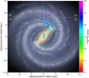 |
Fig. 11 Distribution of 32S/34S ratios from 112 sources in the Milky Way. The background image is the structure of the Milky Way from the artist's impression (Credit: NASA/JPL-Caltech/ESO/R. Hurt). The 32S/34S isotope ratios with corrections of opacity derived in this work from 13CS/13C34S and the double isotope method in the J = 2−1 transition are plotted as circles and stars, respectively. The triangles indicate the results from the CMZ obtained by Humire et al. (2020). The red symbol ⊙ indicates the position of the Sun. The color bar on the right-hand side indicates the range of the 32S/34S ratios. |
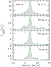 |
Fig. 12 Line proflies of the J = 2−1 transitions of CS, C33S, C34S, and 13CS toward Orion-KL. |
4.4 C36S
As mentioned in Sect. 3.6, we find novel potential indications for a positive 34S/36S gradient with galactocentric radius. The 36S-bearing molecule C36S was first detected by Mauersberger et al. (1996). These authors observed the J = 2−1 and 3−2 transitions toward eight Galactic molecular hot cores at galactocentric distances of between 5.0 kpc and 10.0 kpc. Mauersberger et al. (1996) reported an average 34S/36S ratio of 115 + 17, which is smaller than the value in the Solar System (200.5, Anders & Grevesse 1989). This is consistent with this nucleus being of a purely secondary nature. Combining the ratios of Mauersberger et al. (1996) – after applying new distances (see details in Table 5) – with our results in the J = 2−1 transition, the following fit could be achieved:
 (18)
(18)
with a correlation coefficient of 0.71. As the 34S/33S ratios show a uniform distribution across our Galaxy (see details in Sect. 4.3), a 33S/36S gradient is also expected. We obtain (2.38 + 0.67)/RGC+(13.21 + 4.48). After applying our 32S/34S gradient to the 34S/36S ratios in Mauersberger et al. (1996) with Eq. (9), 32S/36S ratios were then derived and listed in Table 5. Combined with our results in the J = 2−1 transition, a linear fit to the 32S/36S ratios is obtained:
 (19)
(19)
with a correlation coefficient of 0.84. The 34S/36S and 32S/36S ratios are plotted as functions of galactocentric distances in Fig. 9. Measurements of 34S/36S, 33S/36S, and 32S/36S are still not numerous. More sources with detected C36S lines would be highly desirable, especially in the CMZ and the inner disk within RGC = 5.0 kpc.
4.5 Observational bias due to distance effects
While we have so far analyzed isotope ratios as a function of galactocentric distances, there might be a bias in the sense that the ratios could at least in part also depend on the distance from Earth, a bias caused by different linear resolutions. In Appendix B, the 12C/13C, 32S/34S, 34S/33S, and 32S/33S, as well as the 34S/36S and 32S/36S isotope ratios are plotted as functions of the distance from the Sun and shown in Figs. B.2 to B.5, respectively. No apparent gradients can be found, which indicates that any observational bias on account of distance-dependent effects is not significant for 12C/13C, 32S/34S, 32S/33S, 34S/36S, and 32S/36S. This agrees with the findings of Yu et al. (2020, see their Sect. 4.5).
4.6 Beam size effects
A good way to check whether the different beam sizes for different lines could affect our results is to compare the isotope ratios derived from different transitions at different frequencies observed with different beam sizes. As shown in Sect. 3.3, 32S/34S ratios obtained from the double isotope method in the J = 2−1 and 3−2 transitions are in good agreement, suggesting that the effect of beam size is negligible. Furthermore, Humire et al. (2020) found an average 32S/34S ratio of 17.9 + 5.0 in the envelope of Sgr B2(N) with the Atacama Large Millimetre/submillimetre Array (ALMA) with 1".6 beam size, which is consistent with our results in the CMZ from the IRAM 30 meter telescope with beam sizes of about 27". Yu et al. (2020) derived similar 32S/34S and 34S/33S ratios from different telescopes – that is, the IRAM 30 meter and the ARO 12 meter – toward six HMS-FRs and concluded that beam-size effects are insignificant (see details in their Sect. 4.1). All this suggests that beam-size effects could not obviously affect our results.
4.7 Chemical fractionation
Isotopic fractionation could possibly affect the isotope ratios derived from the molecules in the interstellar medium. Watson et al. (1976) firstly proposed that gas-phase CO should have a tendency to be enriched in 13CO because of the charge-exchange reaction of CO with 13C+. Several theoretical studies also support this mechanism (e.g., Langer et al. 1984; Viti et al. 2020), which was then extended to other carbon bearing species (Loison et al. 2020). Formaldehyde forming in the gas phase is suggested to be depleted in the 13C bearing isotopolog (e.g., Langer et al. 1984). However, if H2CO originates from dust grain mantles, then the 13C bearing isotopolog might be enhanced relative to species like methanol and CO (Wirström et al. 2012; Yan et al. 2019). Recently, Colzi et al. (2020) performed a new gas-grain chemical model and proposed that molecules formed starting from atomic carbon could also show 13C enhancements through the reaction 13C + C3 → 12C + 13CC2. As already mentioned in Sect. 4.1, the Galactic 12C/13C gradient derived from C34S in this work is in good agreement with previous results based on measurements of CN, C18O, and H2CO. Therefore, chemical fractionation cannot greatly affect the carbon isotope ratios.
To date, little is known about sulfur fractionation. Loison et al. (2019) proposed a low 34S enrichment through the reaction of 34S+ + CS → S+ + C34S in dense clouds. A slight enrichment in 13C was predicted for CS with the 13C+ +CS → C+ + 13CS reaction (Loison et al. 2020). 32S/34S ratios derived directly from 13CS and 13C34S and the double isotope method involving 12C/13C ratios (Eq. (8)) turn out to agree very well, suggesting that sulfur fractionation is negligible as previously suggested by Humire et al. (2020) and in this work.
Comparison of isotope ratios at different galactocentric distances. Given are percentage enhancements.
4.8 Interstellar C, N, O, and S isotope ratios
The data collected so far allow us to evaluate the status of several isotopes with respect to primary or secondary synthesis in stellar objects. From the data presented here in Table 7, we choose the 12C/13C, 32S/34S, 32S/33S, and 32S/36S ratios because 12C is mostly primary (Timmes et al. 1995) while 32S is definitely a primary nucleus (Woosley & Weaver 1995), against which the other isotopes can be evaluated. A question arises as to whether all these ratios, as well as those from nitrogen and oxygen, can be part of the same scheme.
Comparing the CMZ with the ratios in the inner disk, the CMZ with the outer Galaxy, the inner disk with the ratios in the outer Galaxy, and the local ISM values with those of the Solar System, we obtain increases in values for 12C/13C, 32S/34S, 32S/33S, and 32S/36S ratios. All of these values are listed in Table 9. Percentages are clearly highest between 32S and 36S. These indicate that 36S is, as opposed to 32S, definitely secondary. Percentages between 12C and 13C are also high but not as extreme, presumably because 12C is also synthesized in longer lived stars of intermediate mass (e.g., Kobayashi et al. 2020). More difficult to interpret are the 32S/33S and 32S/34S ratios, where percentages are smaller, indicating that 33S and 34S are, as already mentioned in Sect. 4.3, neither fully primary nor secondary. However, percentages in the case of the 32S/33S ratio systematically surpass those of the 32S/34S ratio, suggesting a more secondary origin of 33S with respect to 34S, even though 34S/33S appears to be constant across the Galaxy. Finally, local interstellar 32S/34S and 32S/33S ratios behave strikingly differently with respect to solar values. While 32S/34S is (almost) solar, 32S/33S is far below the solar value. Peculiar Solar System abundance ratios may be the easiest way to explain this puzzling situation. Most likely there is an overabundance of 34S in the gas and dust that formed the Solar System.
Another clearly primary isotope is 16O, which allows us to look for 16O/18O and 16O/17O ratios (Henkel & Mauersberger 1993; Henkel et al. 1994; Wilson 1999; Wouterloot etal. 2008; Zhang et al. 2020a). The high percentages in the 16O/17O ratios show that 17O is more secondary than 18O, which is consistent with models of stellar nucleosynthesis, because 17O is a main product of the CNO cycle while 18O can also be synthesized by helium burning in massive stars.
14N/15N can also be measured; both nuclei can be synthesized in rotating massive stars and AGB stars as primary products (e.g., Meynet & Maeder 2002; 2011, 2020; Limongi & Chieffi 2018). However, most of the 14N is produced through CNO cycling, and is therefore secondary (e.g., Kobayashi et al. 2011; Karakas & Lattanzio 2014). The production of15 N remains to be understood and may be related to novae (e.g., Kobayashi et al. 2020; Romano 2022). None of the stable nitrogen isotopes are purely primary. While 14N appears to be less secondary than 15N (Audouze et al. 1975; Henkel et al. 1994; Wilson 1999; Adande & Ziurys 2012; Ritchey et al. 2015; Colzi et al. 2018; Chen et al. 2021), in this case we do not have a clear calibration against an isotope that can be considered to be mainly primary. Remarkably, Colzi et al. (2022) reported a rising 14N/N gradient that peaks at RGC = 11 kpc and then decreases, and suggested that 15N could be mainly produced by novae on long timescales.
4.9 Galactic chemical environment
Kobayashi et al. (2020) established a Galactic chemical evolution (GCE) model based on the GCE model in Kobayashi et al. (2011) with updates with respect to new solar abundances and also accounting for failed supernovae, super-AGB stars, the s-process from AGB stars, and various r-process sites. Based on this GCE model, the predicted 12C/13C, 32S/34S, 32S/33S, and 32S/36S ratios at RGC = 2.0, 4.0, 6.0, 8.5, 12.0, and 17.0 kpc are obtained and plotted in Figs. 3, 4, 7, and 9. The initial mass function and nucleosynthesis yields are the same for different galactic radii but star formation and inflow timescales (τs and τi) depend on the Galactic radius (see Kobayashi et al. 2000 for the definition of the timescales). Adopted values are τs = 1.0, 2.0, 3.0, 4.6, 6.5, and 8.8 Gyr as well as τi = 4.0, 5.0, 5.0, 5.0, 7.0, and 50.0 Gyr for RGC = 2.0, 4.0, 6.0, 8.5, 12.0, and 17.0 kpc, respectively. The predicted 12C/13C ratios are in good agreement with our results, while 32S/34S and 32S/36S ratios show significant deviations at larger galactocentric distances. 32S/33S ratios show an offset along the entire inner 12 kpc of the Milky Way. This indicates that current models of Galactic chemical evolution are still far from perfect. In this context, our data will serve as a useful guideline for further even more refined GCE models.
Very recently, Colzi et al. (2022) predicted 12C/13C gradients with four different models addressing nova systems (see details in their Table 2 and Sect. 4), following Romano et al. (2017, 2019, 2021). The gradients from these four models are shown in Fig. 13. The results from model 1 show a large deviation with respect to the observed values. The other three models could reproduce the ratios within the dispersion at galactocentric radii beyond the solar neighborhood, while the inner Galaxy is not as well reproduced.
5 Summary
We used the IRAM 30 meter telescope to perform observations of the J = 2−1 transitions of CS, C33S, C34S, C36S, 13CS, 13C33S, and 13C34S as well as the J = 3−2 transitions of C33S, C34S, C36S, and 13CS toward a large sample of 110 HMSFRs. The CS J = 2−1 line was detected toward 106 sources, with a detection rate of 96%. The J = 2−1 transitions of C34S, 13CS, C33S, 13C34S, and C36S were successfully detected in 90, 82, 46, 17, and 3 of our sources, respectively. The J = 3−2 lines of C34S, 13CS, C33S, and C36S were detected in 87, 71, 42, and 1 object(s). All the detected rare CS isotopologs exhibit optically thin lines and allow us to measure the isotope ratios of 12C/13C, 32S/34S,32S/33S, 32S/36S, 34S/33S, 34S/36S, and 33S/36S with only minor saturation corrections. Our main results are as follows:
Based on the measurements of C34S and 13C34S J = 2−1 transitions, we directly measured the 12C/13C ratios with corrections of opacity. With accurate distances obtained from parallax data (Reid et al. 2009, 2014, 2019), we confirm the previously determined 12C/13C gradient. A least-squares fit to our data results in 12C/13C = (4.77 + 0.81)RGC + (20.76 + 4.61), with a correlation coefficient of 0.82.
The Galactic 12C/13C gradients derived based on measurements of CN (Savage et al. 2002; Milam et al. 2005), C18O (Langer & Penzias 1990; Wouterloot & Brand 1996; Keene et al. 1998), and H2CO (Henkel et al. 1980, 1982, 1983, 1985; Yan et al. 2019) are in agreement with our results from C34S and emphasize that chemical fractionation has little effect on 12C/13C ratios.
While previously it had been assumed that a linear fit would provide a good simulation of carbon isotope ratios as a function of galactocentric distance, our analysis reveals that this does not hold for the Galactic center region. While 12C/13C ratios are lowest in this part of the Milky Way, they clearly surpass values expected from a linear fit to the Galactic disk sources. This indicates that there is no strict linear correlation of carbon isotope ratios across the Galaxy.
We confirm the previously determined 32S/34S gradients (Chin et al. 1996; Yu et al. 2020; Humire et al. 2020) with the direct method from 13CS and 13C34S, as well as the double isotope method also using 12C/13C ratios in the J = 2−1 and J = 3−2 transitions. Opacity corrections could be applied to the J = 2−1 transitions, but not to the J = 3−2 lines that may show, on average, slightly higher opacities. A 32S/34S gradient of (0.75 + 0.13)RGC+(15.52 + 0.78) was obtained based on a large dataset of 90 values from our double isotope method in the J = 2−1 transition. The 19 sources permitting the direct determination of this ratio with 13CS/13C34S yield and should be used as input for further chemical models: (a) In the inner disk the 12C/13C ratios at RGC ≥ 4.0 kpc are clearly higher than the value in the CMZ, while the 32S/34S ratios in the CMZ and inner disk are similar, as already suggested for the first time by Humire et al. (2020). (b) In the local ISM, the 12C/13C ratio is well below the Solar System value but 32S/34S is still quite close to it. All of this indicates that, unlike 13C, 34S is not a clean secondary isotope.
There is no notable 34S/33S gradient across the Galaxy. Ratios are well below the values commonly reported in earlier publications. This is a consequence of accounting for the full hyperfine structure splitting of the C33S lines. The average value of 34S/33S derived from the J = 2−1 transition lines after corrections for opacity toward our sample is 4.35 ± 0.44.
While there is no 34S/33S gradient with galactocentric radius, interstellar 34S/33S values near the solar neighborhood are well below the Solar System ratio, most likely suggesting the Solar System ratio is peculiar, and perhaps also the 18O/17O ratio. A comparison of local interstellar and Solar System 32S/34S and 34S/33S ratios suggests that the Solar System may have been formed from gas and dust with a peculiarly high 34S abundance. The data also indicate that33S is not a clean primary or secondary product of nucleosynthesis, similarly to 34S.
For the first time, we report a 32S/33S gradient in our Galaxy: 32S/33S = (2.64 + 0.77)RGC + (70.80 + 5.57), with a correlation coefficient of 0.46.
We find first potential indications for a positive 34S/36S gradient with galactocentric radius. Combined 34S/36S ratios from Mauersberger et al. (1996) and our new data with corrections of opacity in the J = 2−1 transition and applying new up-to-date distances yield a linear fit of 34S/36S = (10.34 ± 2.74)RGC + (57.45 ± 18.59), with a correlation coefficient of 0.71. Considering the uniform 34S/33S ratios in our Galaxy, a 33S/36S gradient of (2.38 ± 0.67)RGC+(13.21 ± 4.48) is also obtained.
For the first time, we report a tentative 32S/36S gradient with galactocentric radius: 32S/36S = (314 ± 55)RGC ± (659 ± 374), with a correlation coefficient of 0.84. Our measurements are consistent with 36S being a purely secondary nucleus. However, observations of 34S/36S and 32S/36S isotope ratios are still relatively few, especially in the CMZ and the inner disk within RGC = 5.0 kpc.
The predicted 12C/13C ratios from the latest Galactic chemical evolution models (e.g., Kobayashi et al. 2020; Romano et al. 2021; Colzi et al. 2022) are in good agreement with our results, while 32S/34S and 32S/36S ratios show significant differences at larger galactocentric distances. 32S/33S ratios even show clear offsets along the entire inner 12 kpc of the Milky Way. Taken together, these findings provide useful guidelines for further refinements of models of the chemical evolution of the Galaxy.
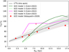 |
Fig. 13 12C/13C isotope ratios from observations in this work and GCE models. The red symbol ⊙ indicates the 12C/13C isotope ratio of the Sun. The 12C/13C gradient obtained from C34S in the current work is plotted as a black solid line, with the gray shaded area showing the 1 σ interval of the fit. The red crosses visualize the results from the GCE model of Kobayashi et al. (2011, 2020, see also Sect. 4.9). The dark green, light green, magenta, and pink lines refer to the predicted gradients from models in Table 2 from Colzi et al. (2022). |
Acknowledgements
We wish to thank the referee for useful comments. Y.T.Y, is a member of the International Max Planck Research School (IMPRS) for Astronomy and Astrophysics at the Universities of Bonn and Cologne. Y.T.Y, would like to thank the China Scholarship Council (CSC) and the Max-Planck-Institut für Radioastronomie (MPIfR) for the financial support. Y.T.Y, also thanks his fiancee, Siqi Guo, for her support during this pandemic period. C.K. acknowledges funding from the UK Science and Technology Facility Council through grant ST/R000905/1 and ST/V000632/1. The work was also partly funded by a Leverhulme Trust Research Project Grant on "Birth of Elements". We thank the IRAM staff for help provided during the observations.
Appendix A Additional Tables
Source list.
32S/34S isotope ratios derived through the double isotope method with the J = 2−1 and J = 3−2 transitions of C34S and 13CS.
Line Parameters derived from Gaussian-fitting.
Appendix B Additional Figures
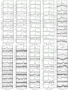 |
Fig. B.1 Line profiles of the J = 2−1 transitions of CS, C33S, C34S, C36S, 13CS, 13C33S and 13C34S as well as the J = 3−2 transitions of C33S, C34S, C36S, and 13CS toward 110 targets of our sample, after subtracting first-order polynomial baselines. The main beam temperature scales are presented on the left hand side of the profiles. |
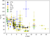 |
Fig. B.2 12C/13C isotope ratios from C34S/13C34S, CN/13CN, C18O/13C18O, |

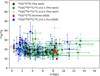 |
Fig. B.3 32S/34S isotope ratios plotted as a function of the distance from the Sun. The symbol Θ indicates the 32S/34S isotope ratio in the Solar System. The 32S/34S ratios with corrections of opacity in the J = 2−1 transition derived from 13CS/13C34S and obtained from the double isotope method are plotted as black and green dots, respectively. The 32S/34S ratios without corrections for optical depth in the J = 3−2 transition derived from the double isotope method are shown as light blue dots. The 32S/34S ratios in Yu et al. (2020) derived from the double isotope method in the J = 2−1 transitions are shown as blue dots. The 32S/34S values in the CMZ obtained from 13CS/13C34S in Humire et al. (2020) are plotted as red stars. |
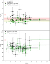 |
Fig. B.4 34S/33S and 32S/33S isotope ratios plotted as functions of the distance from the Sun. Top: 34S/33S ratios derived from C34S/C33S in the J = 2−1 and J = 3−2 transitions are plotted as black and green dots, respectively. The red solid and the two dashed lines show the average value and its standard deviation, 4.35 ± 0.44, for 34S/33S with corrections of optical depth toward our sample in the J = 2−1 transition. The yellow solid and the two dashed lines show the average value and its standard deviation, 3.49 ± 0.26, of 34S/33S toward our sample without opacity corrections for the J = 3−2 transition. The red symbol Θ indicates the 34S/33S isotope ratio in the Solar System. Bottom: Black and green dots show the 32S/33S ratios in the J = 2−1 and J = 3−2 transitions, respectively. The red symbol Θ indicates the 32S/33S value in the Solar System. |
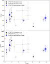 |
Fig. B.5 34S/36S and 32S/36S isotope ratios plotted as functions of the distance from the Sun. Top: Filled black circles and filled black triangle present the 34S/36S ratios in the J = 2−1 and J = 3−2 transitions derived from C34S/C36S in this work with detections of C36S, respectively. The open gray circles and open gray triangles present the 34S/36S ratios in the J = 2−1 and J = 3−2 transitions derived from C34S/C36S in this work with tentative detections of C36S, respectively. The blue diamonds show the 34S/36S ratios in Mauersberger et al. (1996). The red symbol ⊙ indicates the 34S/36S isotope ratio in the Solar System. Bottom: 32S/36S ratios obtained from 34S/36S ratios combined with the 32S/34S ratios derived in this work. The filled black circles and filled black triangle present the values in the J = 2−1 and J = 3−2 transitions from this work with detections of C36S, respectively. The open gray circles and open gray triangles present the ratios in the J = 2−1 and J = 3−2 transitions derived from this work with tentative detections of C36S, respectively. The 32S/36S ratios, derived with 34S/36S values in Mauersberger et al. (1996) and the 32S/34S gradient in this work, are plotted as blue diamonds. The red symbol ⊙ indicates the 32S/36S isotope ratio in the Solar System. |
References
- Adande, G. R., & Ziurys, L. M. 2012, ApJ, 744, 194 [NASA ADS] [CrossRef] [Google Scholar]
- Anders, E., & Grevesse, N. 1989, Geochim. Cosmochim. Acta, 53, 197 [Google Scholar]
- Audouze, J., Lequeux, J., & Vigroux, L. 1975, A&A, 43, 71 [NASA ADS] [Google Scholar]
- Belloche, A., Müller, H. S. P., Menten, K. M., Schilke, P., & Comito, C. 2013, A&A, 559, A47 [NASA ADS] [CrossRef] [EDP Sciences] [Google Scholar]
- Bogey, M., Demuynck, C., & Destombes, J. L. 1981, Chem. Phys. Lett., 81, 256 [NASA ADS] [CrossRef] [Google Scholar]
- Chen, J. L., Zhang, J. S., Henkel, C., et al. 2021, ApJS, 257, 39 [NASA ADS] [CrossRef] [Google Scholar]
- Chiappini, C., Matteucci, F., & Romano, D. 2001, ApJ, 554, 1044 [NASA ADS] [CrossRef] [Google Scholar]
- Chin, Y. N., Henkel, C., Whiteoak, J. B., Langer, N., & Churchwell, E. B. 1996, A&A, 305, 960 [NASA ADS] [Google Scholar]
- Colzi, L., Fontani, F., Caselli, P., et al. 2018, A&A, 609, A129 [NASA ADS] [CrossRef] [EDP Sciences] [Google Scholar]
- Colzi, L., Sipilä, O., Roueff, E., Caselli, P., & Fontani, F. 2020, A&A, 640, A51 [NASA ADS] [CrossRef] [EDP Sciences] [Google Scholar]
- Colzi, L., Romano, D., Fontani, F., et al. 2022, A&A, 667, A151 [NASA ADS] [CrossRef] [EDP Sciences] [Google Scholar]
- Denis-Alpizar, O., Stoecklin, T., Guilloteau, S., & Dutrey, A. 2018, MNRAS, 478, 1811 [Google Scholar]
- Endres, C. P., Schlemmer, S., Schilke, P., Stutzki, J., & Müller, H. S. P. 2016, J. Mol. Spectrosc., 327, 95 [NASA ADS] [CrossRef] [Google Scholar]
- Fontani, F., Caselli, P., Palau, A., Bizzocchi, L., & Ceccarelli, C. 2015, ApJ, 808, L46 [NASA ADS] [CrossRef] [Google Scholar]
- Gardner, F. F., & Whiteoak, J. B. 1981, MNRAS, 194, 37P [NASA ADS] [Google Scholar]
- Gong, Y., Belloche, A., Du, F. J., et al. 2021, A&A, 646, A170 [NASA ADS] [CrossRef] [EDP Sciences] [Google Scholar]
- GRAVITY Collaboration (Abuter, R., et al.) 2019, A&A, 625, A10 [NASA ADS] [CrossRef] [EDP Sciences] [Google Scholar]
- Güsten, R., Henkel, C., & Batrla, W. 1985, A&A, 149, 195 [NASA ADS] [Google Scholar]
- Halfen, D. T., Woolf, N. J., & Ziurys, L. M. 2017, ApJ, 845, 158 [Google Scholar]
- Henkel, C., & Mauersberger, R. 1993, A&A, 274, 730 [NASA ADS] [Google Scholar]
- Henkel, C., Walmsley, C. M., & Wilson, T. L. 1980, A&A, 82, 41 [NASA ADS] [Google Scholar]
- Henkel, C., Wilson, T. L., & Bieging, J. 1982, A&A, 109, 344 [NASA ADS] [Google Scholar]
- Henkel, C., Wilson, T. L., Walmsley, C. M., & Pauls, T. 1983, A&A, 127, 388 [NASA ADS] [Google Scholar]
- Henkel, C., Guesten, R., & Gardner, F. F. 1985, A&A, 143, 148 [Google Scholar]
- Henkel, C., Wilson, T. L., Langer, N., Chin, Y. N., & Mauersberger, R. 1994, Interstellar CNO Isotope Ratios, eds. T. L. Wilson, & K. J. Johnston, 439, 72 [NASA ADS] [Google Scholar]
- Humire, P. K., Thiel, V., Henkel, C., et al. 2020, A&A, 642, A222 [NASA ADS] [CrossRef] [EDP Sciences] [Google Scholar]
- Jacob, A. M., Menten, K. M., Wiesemeyer, H., et al. 2020, A&A, 640, A125 [EDP Sciences] [Google Scholar]
- Karakas, A. I., & Lattanzio, J. C. 2014, PASA, 31, e030 [NASA ADS] [CrossRef] [Google Scholar]
- Keene, J., Schilke, P., Kooi, J., et al. 1998, ApJ, 494, L107 [NASA ADS] [CrossRef] [Google Scholar]
- Kobayashi, C., Tsujimoto, T., & Nomoto, K. 2000, ApJ, 539, 26 [NASA ADS] [CrossRef] [Google Scholar]
- Kobayashi, C., Karakas, A. I., & Umeda, H. 2011, MNRAS, 414, 3231 [Google Scholar]
- Kobayashi, C., Karakas, A. I., & Lugaro, M. 2020, ApJ, 900, 179 [Google Scholar]
- Langer, N. 1989, A&A, 210, 93 [NASA ADS] [Google Scholar]
- Langer, W. D., & Penzias, A. A. 1990, ApJ, 357, 477 [Google Scholar]
- Langer, W. D., & Penzias, A. A. 1993, ApJ, 408, 539 [NASA ADS] [CrossRef] [Google Scholar]
- Langer, W. D., Graedel, T. E., Frerking, M. A., & Armentrout, P. B. 1984, ApJ, 277, 581 [Google Scholar]
- Li, H.-K., Zhang, J.-S., Liu, Z.-W., et al. 2016, Res. Astron. Astrophys., 16, 47 [NASA ADS] [Google Scholar]
- Limongi, M., & Chieffi, A. 2018, ApJS, 237, 13 [NASA ADS] [CrossRef] [Google Scholar]
- Linke, R. A., & Goldsmith, P. F. 1980, ApJ, 235, 437 [Google Scholar]
- Loison, J.-C., Wakelam, V., Gratier, P., et al. 2019, MNRAS, 485, 5777 [Google Scholar]
- Loison, J.-C., Wakelam, V., Gratier, P., & Hickson, K. M. 2020, MNRAS, 498, 4663 [Google Scholar]
- Mauersberger, R., Henkel, C., Langer, N., & Chin, Y. N. 1996, A&A, 313, L1 [Google Scholar]
- Mauersberger, R., Ott, U., Henkel, C., Cernicharo, J., & Gallino, R. 2004, A&A, 426, 219 [NASA ADS] [CrossRef] [EDP Sciences] [Google Scholar]
- Meibom, A., Krot, A. N., Robert, F., et al. 2007, ApJ, 656, L33 [NASA ADS] [CrossRef] [Google Scholar]
- Menten, K. M., Reid, M. J., Forbrich, J., & Brunthaler, A. 2007, A&A, 474, 515 [NASA ADS] [CrossRef] [EDP Sciences] [Google Scholar]
- Meyer, B. S. 1994, ARA&A, 32, 153 [NASA ADS] [CrossRef] [Google Scholar]
- Meynet, G., & Maeder, A. 2002, A&A, 390, 561 [NASA ADS] [CrossRef] [EDP Sciences] [Google Scholar]
- Milam, S. N., Savage, C., Brewster, M. A., Ziurys, L. M., & Wyckoff, S. 2005, ApJ, 634, 1126 [Google Scholar]
- Müller, H. S. P., Schlöder, F., Stutzki, J., & Winnewisser, G. 2005, J. Mol. Struct., 742, 215 [Google Scholar]
- Pilkington, K., Few, C. G., Gibson, B. K., et al. 2012, A&A, 540, A56 [NASA ADS] [CrossRef] [EDP Sciences] [Google Scholar]
- Reid, M. J., Menten, K. M., Zheng, X. W., et al. 2009, ApJ, 700, 137 [CrossRef] [Google Scholar]
- Reid, M. J., Menten, K. M., Brunthaler, A., et al. 2014, ApJ, 783, 130 [Google Scholar]
- Reid, M. J., Menten, K. M., Brunthaler, A., et al. 2019, ApJ, 885, 131 [Google Scholar]
- Riquelme, D., Amo-Baladrón, M. A., Martín-Pintado, J., et al. 2010, A&A, 523, A51 [NASA ADS] [CrossRef] [EDP Sciences] [Google Scholar]
- Ritchey, A. M., Federman, S. R., & Lambert, D. L. 2011, ApJ, 728, 36 [NASA ADS] [CrossRef] [Google Scholar]
- Ritchey, A. M., Federman, S. R., & Lambert, D. L. 2015, ApJ, 804, L3 [NASA ADS] [CrossRef] [Google Scholar]
- Roman-Duval, J., Jackson, J. M., Heyer, M., et al. 2009, ApJ, 699, 1153 [CrossRef] [Google Scholar]
- Romano, D. 2022, A&AR, 30, 7 [NASA ADS] [CrossRef] [Google Scholar]
- Romano, D., Matteucci, F., Zhang, Z. Y., Papadopoulos, P. P., & Ivison, R. J. 2017, MNRAS, 470, 401 [NASA ADS] [CrossRef] [Google Scholar]
- Romano, D., Matteucci, F., Zhang, Z.-Y., Ivison, R. J., & Ventura, P. 2019, MNRAS, 490, 2838 [NASA ADS] [CrossRef] [Google Scholar]
- Romano, D., Magrini, L., Randich, S., et al. 2021, A&A, 653, A72 [NASA ADS] [CrossRef] [EDP Sciences] [Google Scholar]
- Savage, C., Apponi, A. J., Ziurys, L. M., & Wyckoff, S. 2002, ApJ, 578, 211 [NASA ADS] [CrossRef] [Google Scholar]
- Thielemann, F. K., & Arnett, W. D. 1985, ApJ, 295, 604 [NASA ADS] [CrossRef] [Google Scholar]
- Timmes, F. X., Woosley, S. E., & Weaver, T. A. 1995, ApJS, 98, 617 [NASA ADS] [CrossRef] [Google Scholar]
- van der Tak, F. F. S., Black, J. H., Schöier, F. L., Jansen, D. J., & van Dishoeck, E. F. 2007, A&A, 468, 627 [NASA ADS] [CrossRef] [EDP Sciences] [Google Scholar]
- Viti, S., Fontani, F., & Jiménez-Serra, I. 2020, MNRAS, 497, 4333 [NASA ADS] [CrossRef] [Google Scholar]
- Watson, W. D., Anicich, V. G., & Huntress, W. T. J. 1976, ApJ, 205, L165 [NASA ADS] [CrossRef] [Google Scholar]
- Whiteoak, J. B., & Gardner, F. F. 1979, MNRAS, 188, 445 [NASA ADS] [Google Scholar]
- Wilson, T. L. 1999, Rep. Prog. Phys., 62, 143 [Google Scholar]
- Wilson, T. L., & Rood, R. 1994, ARA&A, 32, 191 [Google Scholar]
- Wilson, T. L., Bieging, J., Downes, D., & Gardner, F. F. 1976, A&A, 51, 303 [NASA ADS] [Google Scholar]
- Wirström, E. S., Charnley, S. B., Geppert, W. D., & Persson, C. M. 2012, in 43rd Annual Lunar and Planetary Science Conference, Lunar and Planetary Science Conference, 1611 [Google Scholar]
- Woosley, S. E., & Weaver, T. A. 1995, ApJS, 101, 181 [Google Scholar]
- Wouterloot, J. G. A., & Brand, J. 1996, A&AS, 119, 439 [NASA ADS] [CrossRef] [EDP Sciences] [Google Scholar]
- Wouterloot, J. G. A., Henkel, C., Brand, J., & Davis, G. R. 2008, A&A, 487, 237 [NASA ADS] [CrossRef] [EDP Sciences] [Google Scholar]
- Xu, Y., Reid, M. J., Zheng, X. W., & Menten, K. M. 2006, Science, 311, 54 [NASA ADS] [CrossRef] [Google Scholar]
- Xu, Y., Li, J. J., Reid, M. J., et al. 2013, ApJ, 769, 15 [Google Scholar]
- Yan, Y. T., Zhang, J. S., Henkel, C., et al. 2019, ApJ, 877, 154 [Google Scholar]
- Yu, H. Z., Zhang, J. S., Henkel, C., et al. 2020, ApJ, 899, 145 [NASA ADS] [CrossRef] [Google Scholar]
- Zhang, J. S., Sun, L. L., Riquelme, D., et al. 2015, ApJS, 219, 28 [Google Scholar]
- Zhang, J. S., Liu, W., Yan, Y. T., et al. 2020a, ApJS, 249, 6 [Google Scholar]
- Zhang, J. S., Yan, Y. T., Liu, W., et al. 2020b, in IAU General Assembly, 278 [Google Scholar]
All Tables
Comparison of isotope ratios at different galactocentric distances. Given are percentage enhancements.
32S/34S isotope ratios derived through the double isotope method with the J = 2−1 and J = 3−2 transitions of C34S and 13CS.
All Figures
|
Fig. 1 Line profiles of the J = 2−1 transitions of CS, C33S, C34S, C36S, 13CS, 13C33S, and 13C34S as well as the J = 3−2 transitions of C33S, C34S, C36S, and 13CS toward one typical target (DR21) of our large sample of 110 sources, after subtracting first-order polynomial baselines. The main beam brightness temperature scales are presented on the left hand side of the profiles. The spectra of all 110 objects in our sample are shown in Fig. B.1. |
| In the text | |
|
Fig. 2 Excitation temperature, Tex, as a function of optical depth for the J = 2−1 transition of C34S. The gray dashed lines indicate the range of opacities for our sample sources. |
| In the text | |
|
Fig. 3 12C/13C isotope ratios from C34S/13C34S, CN/13CN, C18O/13C18O, |
| In the text | |
|
Fig. 4 32S/34S isotope ratios as functions of the distance from the Galactic center. The symbol ⊙ indicates the 32S/34S isotope ratio in the Solar System. In the upper panel, the 32S/34S ratios directly derived from 13CS/13C34S in the J = 2−1 transition and obtained from the double isotope method in the J = 2−1 transition with corrections for optical depth are plotted as black and green dots, respectively. The 32S/34S ratios without corrections of opacity in the J = 3−2 transition are plotted as light blue dots. The 3σ lower limits of 32S/34S ratios obtained from non-detections of 13C34S in the current work are shown as open black circles. The 32S/34S ratios in Yu et al. (2020) derived from the double isotope method in the J = 2−1 transitions are shown as blue dots in the lower panel. The 32S/34S values in the CMZ obtained from 13CS/13C34S in Humire et al. (2020) are plotted as red stars in both panels. The resulting first-order polynomial fits to 32S/34S ratios with the direct method and the double isotope method from the J = 2−1 transition in this work are plotted as black and red solid lines in the two panels, respectively, with the gray and yellow shaded areas showing the 1 σ intervals of the fits. The magenta and cyan dashed-dotted lines show the 32S/34S gradients from Chin et al. (1996) and Yu et al. (2020). The red crosses visualize the results from the GCE model of Kobayashi et al. (2011, 2020, see also Sect. 4.9). |
| In the text | |
|
Fig. 5 Synthetic C33S (2−-1) and C33S (3−2) spectra for two intrinsic line widths, 1.0 km s−1 (left panels) and 4.0 km s−1 (right panels). |
| In the text | |
|
Fig. 6 Blue lines are curves showing the theoretical dependencies of the HFS factors, f21HFS (left) and f32HFS (right), on the line width of the C33S main component for sources in which only the main component was detected. The red dotted vertical and horizontal lines indicate the values of the minimal line widths where the factors are reaching almost 1.0, 19.0 km s−1 for the J = 2−1 transition (f21HFS ∼ 0.99) and 9.2 km s−1 for the J = 3−2 transition (f32HFS ∼ 0.99). |
| In the text | |
|
Fig. 7 34S/33S and 32S/33S isotope ratios (for the latter, see Eqs. (12) and (13)) plotted as functions of the distance from the Galactic center. Top: 34S/33S ratios derived from C34S/C33S in the J = 2−1 and J = 3−2 transitions plotted as black and green dots, respectively. The red solid and the two dashed lines show the average value and its standard deviation, 4.35 ± 0.44, of 34S/33S with corrections of optical depth toward our sample in the J = 2−1 transition. The yellow solid and the two dashed lines show the average value and its standard deviation, 3.49 ± 0.26, of 34S/33S toward our sample in the J = 3−2 transition. The red symbol ⊙ indicates the 34S/33S isotope ratio in the Solar System. Bottom: Black and green dots show the 32S/33S ratios in the J = 2−1 and J = 3−2 transitions, respectively. The red symbol ⊙ indicates the 32S/33S value in the Solar System. The resulting first-order polynomial fits to the 32S/33S ratios in the J = 2−1 and J = 3−2 transitions in this work are plotted as red and green solid lines, respectively, with the pink and yellow shaded area showing the 1 σ standard deviations. The red crosses are the results from the GCE model of Kobayashi et al. (2011, 2020, see also Sect. 4.9). |
| In the text | |
|
Fig. 8 Comparison of 34S/33S ratios between the J = 2−1 and 3−2 data. The J = 2−1 ratios are opacity corrected, while the same correction factors were also applied to the J = 3−2 data. The red solid line indicates that the 34S/33S ratios are equal in these two transitions. |
| In the text | |
|
Fig. 9 J = 2−1 (opacity corrected) and J = 32 (no opacity corrections) 34S/36S and 32S/36S isotope ratios (see Eqs. (18) and (19)) plotted as functions of the distance from the Galactic center. Top: Filled black circles and filled black triangle present the 34S/36S ratios in the J = 2−1 and J = 3−2 transitions derived from C34S/C36S in this work with detections of C36S, respectively. The open gray circles and open gray triangles present the 34S/36S ratios in the J = 2−1 and J = 3−2 transitions derived from C34S/C36S in this work with tentative detections of C36S, respectively. The blue diamonds show the 34S/36S ratios in Mauersberger et al. (1996). The red symbol ⊙ indicates the 34S/36S isotope ratio in the Solar System. The resulting first-order polynomial fit to the 34S/36S ratios in Mauersberger et al. (1996) and this work, excluding the values from tentative detections, is plotted as a black solid line, with the green shaded area showing the 1 σ interval of the fit. Bottom: 32S/36S ratios obtained from 34S/36S ratios combined with the 32S/34S ratios derived in this work. The filled black circles and filled black triangle present the values in the J = 2−1 and J = 3−2 transitions from this work with detections of C36S, respectively. The open gray circles and open gray triangles present ratios in the J = 2−1 and J = 3−2 transitions from this work with tentative detections of C36S, respectively. The 32S/36S ratios derived with 34S/36S values from Mauersberger et al. (1996) are plotted as blue diamonds. The red symbol ⊙ indicates the 32S/36S isotope ratio in the Solar System. The 32S/36S gradient, excluding tentative detections, is plotted as a black solid line, with the pink shaded area showing the 1 σ interval of the fit. The red crosses visualize results from the GCE model of Kobayashi et al. (2011, 2020, see Sect. 4.9). |
| In the text | |
|
Fig. 10 Distribution of 12C/13C ratios from 93 sources in the Milky Way. The background image is the structure of the Milky Way from the artist's impression [Credit: NASA/JPL-Caltech/ESO/R. Hurt]. The 12C/13C isotope ratios with corrections for optical depth from C34S/13C34S in this work are plotted as circles. The triangles, pentagons, stars, squares, and diamonds indicate the 12C/13C ratios derived from CN/13CN (Savage et al. 2002; Milam et al. 2005), C18O/13C18O (Langer & Penzias 1990; Wouterloot & Brand 1996; Keene et al. 1998), |
| In the text | |
|
Fig. 11 Distribution of 32S/34S ratios from 112 sources in the Milky Way. The background image is the structure of the Milky Way from the artist's impression (Credit: NASA/JPL-Caltech/ESO/R. Hurt). The 32S/34S isotope ratios with corrections of opacity derived in this work from 13CS/13C34S and the double isotope method in the J = 2−1 transition are plotted as circles and stars, respectively. The triangles indicate the results from the CMZ obtained by Humire et al. (2020). The red symbol ⊙ indicates the position of the Sun. The color bar on the right-hand side indicates the range of the 32S/34S ratios. |
| In the text | |
|
Fig. 12 Line proflies of the J = 2−1 transitions of CS, C33S, C34S, and 13CS toward Orion-KL. |
| In the text | |
|
Fig. 13 12C/13C isotope ratios from observations in this work and GCE models. The red symbol ⊙ indicates the 12C/13C isotope ratio of the Sun. The 12C/13C gradient obtained from C34S in the current work is plotted as a black solid line, with the gray shaded area showing the 1 σ interval of the fit. The red crosses visualize the results from the GCE model of Kobayashi et al. (2011, 2020, see also Sect. 4.9). The dark green, light green, magenta, and pink lines refer to the predicted gradients from models in Table 2 from Colzi et al. (2022). |
| In the text | |
|
Fig. B.1 Line profiles of the J = 2−1 transitions of CS, C33S, C34S, C36S, 13CS, 13C33S and 13C34S as well as the J = 3−2 transitions of C33S, C34S, C36S, and 13CS toward 110 targets of our sample, after subtracting first-order polynomial baselines. The main beam temperature scales are presented on the left hand side of the profiles. |
| In the text | |
|
Fig. B.2 12C/13C isotope ratios from C34S/13C34S, CN/13CN, C18O/13C18O, |
| In the text | |
|
Fig. B.3 32S/34S isotope ratios plotted as a function of the distance from the Sun. The symbol Θ indicates the 32S/34S isotope ratio in the Solar System. The 32S/34S ratios with corrections of opacity in the J = 2−1 transition derived from 13CS/13C34S and obtained from the double isotope method are plotted as black and green dots, respectively. The 32S/34S ratios without corrections for optical depth in the J = 3−2 transition derived from the double isotope method are shown as light blue dots. The 32S/34S ratios in Yu et al. (2020) derived from the double isotope method in the J = 2−1 transitions are shown as blue dots. The 32S/34S values in the CMZ obtained from 13CS/13C34S in Humire et al. (2020) are plotted as red stars. |
| In the text | |
|
Fig. B.4 34S/33S and 32S/33S isotope ratios plotted as functions of the distance from the Sun. Top: 34S/33S ratios derived from C34S/C33S in the J = 2−1 and J = 3−2 transitions are plotted as black and green dots, respectively. The red solid and the two dashed lines show the average value and its standard deviation, 4.35 ± 0.44, for 34S/33S with corrections of optical depth toward our sample in the J = 2−1 transition. The yellow solid and the two dashed lines show the average value and its standard deviation, 3.49 ± 0.26, of 34S/33S toward our sample without opacity corrections for the J = 3−2 transition. The red symbol Θ indicates the 34S/33S isotope ratio in the Solar System. Bottom: Black and green dots show the 32S/33S ratios in the J = 2−1 and J = 3−2 transitions, respectively. The red symbol Θ indicates the 32S/33S value in the Solar System. |
| In the text | |
|
Fig. B.5 34S/36S and 32S/36S isotope ratios plotted as functions of the distance from the Sun. Top: Filled black circles and filled black triangle present the 34S/36S ratios in the J = 2−1 and J = 3−2 transitions derived from C34S/C36S in this work with detections of C36S, respectively. The open gray circles and open gray triangles present the 34S/36S ratios in the J = 2−1 and J = 3−2 transitions derived from C34S/C36S in this work with tentative detections of C36S, respectively. The blue diamonds show the 34S/36S ratios in Mauersberger et al. (1996). The red symbol ⊙ indicates the 34S/36S isotope ratio in the Solar System. Bottom: 32S/36S ratios obtained from 34S/36S ratios combined with the 32S/34S ratios derived in this work. The filled black circles and filled black triangle present the values in the J = 2−1 and J = 3−2 transitions from this work with detections of C36S, respectively. The open gray circles and open gray triangles present the ratios in the J = 2−1 and J = 3−2 transitions derived from this work with tentative detections of C36S, respectively. The 32S/36S ratios, derived with 34S/36S values in Mauersberger et al. (1996) and the 32S/34S gradient in this work, are plotted as blue diamonds. The red symbol ⊙ indicates the 32S/36S isotope ratio in the Solar System. |
| In the text | |
Current usage metrics show cumulative count of Article Views (full-text article views including HTML views, PDF and ePub downloads, according to the available data) and Abstracts Views on Vision4Press platform.
Data correspond to usage on the plateform after 2015. The current usage metrics is available 48-96 hours after online publication and is updated daily on week days.
Initial download of the metrics may take a while.