| Issue |
A&A
Volume 667, November 2022
|
|
|---|---|---|
| Article Number | A137 | |
| Number of page(s) | 30 | |
| Section | Interstellar and circumstellar matter | |
| DOI | https://doi.org/10.1051/0004-6361/202244000 | |
| Published online | 18 November 2022 | |
Ammonia characterisation of dense cores in the Rosette Molecular Cloud★
1
Eötvös Loránd University, Department of Astronomy,
Pázmány Péter sétány 1/A,
1117
Budapest, Hungary
e-mail: This email address is being protected from spambots. You need JavaScript enabled to view it.
2
Institut UTINAM, CNRS UMR 6213, OSU THETA, Université de Franche-Comté,
41 bis avenue de l’Observatoire,
25000
Besançon, France
3
Laboratoire d’astrophysique de Bordeaux, Université de Bordeaux, CNRS,
B18N, allée Geoffroy Saint-Hilaire,
33615
Pessac, France
4
Max-Planck-Institut für Radioastronomie,
Auf dem Hügel 69,
53121
Bonn, Germany
5
I. Physikalische Institut, University of Cologne,
Zuelpicher Str. 77,
50937
Cologne, Germany
6
Univ. Grenoble Alpes, CNRS, IPAG,
38000
Grenoble, France
7
University of Debrecen, Faculty of Science and Technology, Institute of Physics,
PO Box 400,
4002
Debrecen, Hungary
Received:
11
May
2022
Accepted:
30
August
2022
Abstract
Context. The Rosette molecular cloud complex is a well-known Galactic star-forming region with a morphology pointing towards triggered star formation. The distribution of its young stellar population and the gas properties point to the possibility that star formation is globally triggered in the region.
Aims. We focus on the characterisation of the most massive pre- and protostellar cores distributed throughout the molecular cloud in order to understand the star formation processes in the region.
Methods. We observed a sample of 33 dense cores, identified in Herschel continuum maps, with the Effelsberg 100-m telescope. Using NH3 (1,1) and (2,2) measurements, we characterise the dense core population, computing rotational and gas kinetic temperatures and NH3 column density with multiple methods. We also estimated the gas pressure ratio and virial parameters to examine the stability of the cores. Using results from Berschel data, we examined possible correlations between gas and dust parameters.
Results. Ammonia emission is detected towards 31 out of the 33 selected targets. We estimate kinetic temperatures to be between 12 and 20 K, and column densities within the 1014−2 × 1015 cm−2 range in the selected targets. Our virial analysis suggests that most sources are likely to be gravitationally bound, while the line widths are dominated by non-thermal motions. Our results are compatible with large-scale dust temperature maps suggesting that the temperature decreases and column density increases with distance from NGC 2244 except for the densest protoclusters. We also identify a small spatial shift between the ammonia and dust peaks in the regions most exposed to irradiation from the nearby NGC 2244 stellar cluster. However, we find no trends in terms of core evolution with spatial location, in the prestellar to protostellar core abundance ratio, or the virial parameter.
Conclusions. Star formation is more likely based on the primordial structure of the cloud in spite of the impact of irradiation from the nearby cluster, NGC 2244. The physical parameters from the NH3 measurements suggest gas properties in between those of low- and high-mass star-forming regions, suggesting that the Rosette molecular cloud could host ongoing intermediate-mass star formation, and is unlikely to form high-mass stars.
Key words: stars: formation / ISM: clouds / ISM: molecules
The reduced spectra are also available at the CDS via anonymous ftp to cdsarc.cds.unistra.fr (130.79.128.5) or via https://cdsarc.cds.unistra.fr/viz-bin/cat/J/A+A/667/A137
© R. Bőgner et al. 2022
 Open Access article, published by EDP Sciences, under the terms of the Creative Commons Attribution License (https://creativecommons.org/licenses/by/4.0), which permits unrestricted use, distribution, and reproduction in any medium, provided the original work is properly cited.
This article is published in open access under the Subscribe-to-Open model. This email address is being protected from spambots. You need JavaScript enabled to view it. to support open access publication.
1 Introduction
Stars form in dense cores within molecular clouds. Although the scenario for the formation of low-mass stars is well established (e.g. Andre et al. 2000), the process of high-mass (>8 M⊙) star formation is still not well understood (for a review see Tan et al. 2014; Motte et al. 2018). Observations in the high-mass range are more challenging because massive stars are more rare according to the stellar initial mass function (e.g. Weidner et al. 2011) and are typically found at larger distances than low-mass star-forming regions. High-mass stars form in clusters in complex, diverse environments and are deeply embedded in their earliest phases (Motte et al. 2018). Nevertheless, they are of special importance for the evolution of galaxies. They energise the interstellar medium (ISM) and enrich it with heavy elements, which influence cooling mechanisms (Kennicutt 2005). Their ionising radiation forms HII regions, and through their strong winds, outflows, and supernova explosions they mix the ISM (Zinnecker & Yorke 2007).
Such mechanical and radiative feedback from newly formed stars could trigger the formation of new generations of stars (Elmegreen 1998; Deharveng et al. 2005), and two main theories are discussed; the collect-and-collapse scenario (Elmegreen & Lada 1977), and radiation-driven implosion (Bertoldi 1989; Lefloch & Lazareff 1994). In the collect-and-collapse scenario, an expanding HII region sweeps up the surrounding material around the HII region to form a shell. This eventually becomes self-gravitating, fragmenting to form dense clumps that can collapse to form stars. As these fragments are massive (a few hundred M⊙), this scenario could explain the hierarchical nature of massive stellar clusters (Bastian et al. 2005). With the radiation-driven implosion, an expanding ionisation front of an HII region drives a shock to the surrounding molecular material, triggering the collapse of present subcritical clumps. The importance of feedback effects can be quantified using a combination of molecular tracers that allow us to measure the thermal pressure in the expanding HII gas, and recent studies heavily rely on [C II], CO and its isotopologues to measure feedback effects (e.g. Schneider et al. 2020; Pabst et al. 2019). To elucidate whether generations of stars could have formed due to triggering, other approaches rely on source counts and clustering of young stellar objects towards HII regions (Cárdenas et al. 2022), which, combined with morphological evidence, could indicate a potential triggered nature of the star formation scenario.
Development of our understanding of stellar feedback in star formation requires either drawing robust statistics from large samples of star-forming regions (e.g. Thompson et al. 2012; Elia et al. 2017, 2021) or characterising a small set of template regions in detail, such as for example the Λ Orionis region (Liu et al. 2016; Yi et al. 2018, 2021), or the massive molecular clouds W43 (Motte et al. 2003), Cygnus X (Motte et al. 2007), or G305 (Mazumdar et al. 2021a,b).
Several case studies emerge for triggering around expanding Galactic bubbles (e.g. Mookerjea 2022), and in this context the Rosette Nebula is an archetypical massive molecular cloud (1.6 × 10⁵ M⊙, Williams et al. 1995; Schneider et al. 1998; Heyer et al. 2006) where the role of triggered star formation is debated. This molecular cloud is associated with the OB cluster, NGC 2244, at its centre, which has approximately 2000 star members, of which 7 are O-type and 24 are B-type stars (Wang et al. 2008). These stars have already disrupted their surrounding medium of the Rosette Molecular Cloud (RMC), producing an expanding HII region inside the molecular cloud. The interaction between the OB stars and the molecular medium produced an extended photon-dominated region at the interface and radiation may also penetrate into the cloud. Recent distance estimates based on Gaia DR2 parallaxes confirm the distance of the Nebula at  pc and
  pc for NGC 2244 (Kuhn et al. 2019).
Using multi-band Herschel data, Schneider et al. (2010) found a temperature gradient for dust that decreases into the molecular cloud with increasing distance from the OB cluster, and could be indicative of an age gradient. Schneider et al. (2012) revisited this scenario and concluded that star formation in the RMC is probably only ‘triggered’ in the direct interface region between the HII region and the molecular cloud. These authors found no indication of sequential star formation; rather that clusters form at the junctions of filaments. The study of Cambrésy et al. (2013) analysed the distribution of the interstellar medium with extinction mapping. They computed young star cluster surface densities and an age estimation that led them to conclude that a triggering scenario for the star formation in the Rosette is not consistent with all the observed cluster ages.
Figure 1 shows an overview of the RMC. Seven clusters of young stellar objects (YSOs) have been identified in the RMC by Phelps & Lada (1997), and we refer to them as PL01–PL07. Román-Zúñiga et al. (2008) found three other clusters, REFL08, REFL09, and REFL10. The two former clusters are associated with massive clumps in the molecular cloud, and the latter is a small cluster at the northeast end of the cloud. Among these, only REFL08 falls inside our area of study, as it was the only cluster out of the three to be included in the previous studies done by Motte et al. (2010) and Schneider et al. (2010, 2012). To define distinct regions of the molecular cloud, we follow the nomenclature of Schneider et al. (2010). These regions along with the clusters are described in Sect. 5.1.
Motte et al. (2010) identified the 46 most massive dense cores (~0.1 pc) of the RMC from Herschel data (open squares in Fig. 1). These authors obtained the evolutionary stage of the sources by searching for point-like Spitzer 24 µm sources within Herschel dense cores. Using spectral energy distributions (SEDs), they determined their masses, luminosities, and dust temperatures. The sample contains 4 warm-starless, 12 prestellar, and 30 protostellar cores with masses ranging from 0.8 to 39 M⊙.
Previous studies of this region mainly focused on its YSO population through near-infrared (NIR) observations (Román-Zúñiga et al. 2008; Poulton et al. 2008), on dust emission (Shipman & Clark 1994; Motte et al. 2010; di Francesco et al. 2010; Schneider et al. 2010), and on intermediate-density gas (CO isotopologues, Veltchev et al. 2018; Li et al. 2018). Gas observations revealed two main velocity components that are rather distinct, around 10 km s−1 and 15 km s−1 (Schneider et al. 1998). The Rosette complex has recently been mapped in NH3 (1,1) and (2,2) inversion transitions using the Green Bank Telescope in the frame of the K-band Focal Plane Array Examinations of Young STellar Object Natal Environments (KEYSTONE) project (Keown et al. 2019). This project provides maps of the NH3 (1,1) and (2,2) inversion transitions with a median rms of 0.16 K per 0.07 km s−1. Using a dendrogram analysis, Keown et al. (2019) identified a sample of dense gas clumps with a total of 48 NH3 leaves towards the RMC, and compared them to the NH3 clump properties of seven other star-forming regions.
NH3 has been shown to be a good tracer of cold dense gas, and the volume density of high-mass star-forming clumps is around the critical density of NH3 at about ~104 cm−3 (Rohlfs & Wilson 2004). Therefore, NH3 is suitable for investigating the physical parameters of such clumps without being affected by confusion from the surrounding lower density large-scale cloud structures. In addition, NH3 is not easily depleted onto dust grains at low temperatures, in contrast to many other molecular tracers such as CO. NH3 is known to be a reliable temperature probe of dense interstellar medium (Ho & Townes 1983; Walmsley & Ungerechts 1983; Ungerechts et al. 1986; Juvela et al. 2012) through its inversion transitions. As the inversion transitions are split into hyperfine components, their ratio can be used to measure the optical depth. From that, one can obtain a reliable column density and rotational temperature estimation which can then be used to calculate the gas kinetic temperature.
In the present paper, we focus on the dense core population of the RMC with single pointing observations of NH3 inversion lines with better sensitivity (Sect. 2.2) than in Keown et al. (2019). Our aim is to characterise the star-forming cores themselves in detail through the emission of the dense gas ( ~ 104 cm−3) in order to examine the physical properties of the dense cores and to correlate them with the tentative age gradient found by Schneider et al. (2010). We also investigate whether feedback effects have an impact on star formation through a comparative analysis of the different regions taking into account their distance to NGC 2244.
The paper is structured as follows. Details on the observation and data reduction are given in Sect. 2. In Sect. 3, we present the derivations of physical parameters from the NH3 data and the results are then presented in Sect. 4. We discuss the implications of our results and compare them to other similar datasets in Sect. 5. Our findings are summarised in Sect. 6.
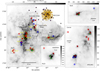 |
Fig. 1 Overview of the Rosette Nebula on a Berschel SPIRE 250 µm surface brightness map. The cores observed at Effelsberg are shown with different colours, which indicate their evolutionary stages derived from Berschel data by Motte et al. (2010): (green) warm-starless, (blue) prestellar, (red) protostellar core. The yellow dots represent the stars of the cluster NGC 2244. The white and purple stars mark the O and B stars of the cluster, respectively. The areas indicated by black rectangles and the YSO clusters indicated by yellow circles are presented in Sect. 1. The inserts give a closer look at areas PL03, Shell, Center, and AFGL 961 in order to clearly distinguish our sources. |
2 Observations
2.1 Sample selection
We selected 33 of the 45 massive dense cores identified by Motte et al. (2010) for NH3 observations with the Effelsberg 100 m telescope (project 89-10). This selection covers 73% of the total number of massive dense cores identified. We first classified the sources into starless and protostellar cores by searching for point-like Spitzer 24 µm sources associated with the Herschel cores. Based on fitting the SED, Motte et al. (2010) also identified a sample of warm starless cores, and defined prestellar cores. In the present project, we targeted all 4 warm starless cores, 9 of the 12 prestellar cores (75%), and 20 of the 29 protostellar cores (69%).
Table 1 shows the parameters obtained from Berschel measurements of the cores by Motte et al. (2010). Performing a grey-body SED fitting, these authors derived dust temperature, mass, and bolometric luminosity for the sample. The masses were estimated assuming optically thin 350 µm emission.
2.2 Effelsberg NH3 observations and data reduction
The NH3 observations were carried out with the Effelsberg 100m telescope in January 2011. We observed the NH3 (1,1) and (2,2) inversion lines at about 24 GHz simultaneously using single pointing observations in frequency switching mode with a frequency throw of 7.5 MHz. We used the K-band receiver frontend and the fast Fourier transform spectrometer (FFTS) backend with a total bandwidth of 100 MHz. We calculate a velocity resolution of 0.08 km s−1 using 3.5 kHz effective spectral resolution at the observing frequency of 23.7 GHz, and we smoothed the data to a resolution of 0.15. Altogether we observed 33 sources with an integration time of 30 minutes for each source. The beam width of the telescope is 40” at the frequencies of the NH3 lines, corresponding to a linear scale of about 0.28 pc at a distance of 1.6 kpc.
The data reduction was performed with the CLASS package of the GILDAS1 software distribution developed by IRAM. We based our data analysis on the method outlined in Wienen et al. (2012). We used a standard calibrator, NGC7027, a planetary nebula which is expected not to show linear polarisation, and whose flux density is precisely known (Ott et al. 1994). The variation of the flux of NGC 7027 is ~0.1% and the variation of the noise diode temperature in our sample was between 4–6%, both being smaller than the average calibration uncertainty of 10%. This allowed us to calculate only one calibration factor for each day of observation from the main beam brightness temperature of NGC 7027 (see also Wienen et al. 2012). Because the frequency switching gives two lines, inverted and separated by 7.5 MHz, this had to be reversed by folding the spectra. It shifted the lines by 3.75 MHz and subtracted them from one another. To correct for the fluctuations in the spectral baseline, we subtracted a polynomial function of the order of 3 to 7, excluding the lines in an iterative way. To fit the NH3 (1,1) lines, we defined windows around each hyperfine component in order to exclude them from the baseline fitting. Because our sources at different evolutionary phases of high-mass star formation show various line profiles as well as line widths, we needed a systematic method to reduce them in the same way. We therefore implemented a pipeline that chooses the width of the window around each (1,1) hyperfine component as well as the order of the baseline dependent on the width of the main line. To define the width of the windows, we made a preliminary method NH3 fit, and multiplied the resulting full width at half maximum (FWHM) values by 1.5. Following this method, the order of the polynomial decreases with increasing line width (cf. Wienen et al. 2012).
We obtain a median rms noise of 60 mK (for a maximum system temperature of 150 K) in TMB scale in a velocity bin of 0.15 km s−1.
We extracted the line parameters using the method NH3 and minimize fitting commands of CLASS. This fitting method assumes that the hyperfine structure (hfs) components have Gaussian profiles and that they all have the same excitation temperature. In this fitting method, the main group opacity is limited to the range of 0.1−30. The independent parameters obtained from the fitting are the radial velocity (vLSR), the FWHM of a Gaussian profile (Δν), and the optical depth of the main line (τm) with their respective errors. From these parameters, we computed the maximum main beam temperature and the signal-to-noise ratio (S/N). The rms of the spectra were obtained from the baseline fitting in CLASS.
The results of the NH3 line fitting are given in Table B.1. In summary, the main hyperfine optical depth varies between 0.1 and 2.05 with an average of 0.75. The NH3 lines are therefore optically thin overall, though we note that the values for τ and Tex are not independent.
The hyperfine satellite lines of the NH3 (2,2) inversion transitions are rather weak, and hence we could not apply the same procedure as for the NH3 (1,1) line. Instead, we fitted a single Gaussian to the main component in CLASS, giving the independent parameters of the integrated area (A), the radial velocity (vLSR), and the FWHM line width (Δν). Consequently, the optical depth of this transition could not be determined. Figure 2 shows an example spectrum of the NH3 (1,1) and (2,2) transitions for core #71 with the results obtained from the CLASS fit. The spectra and their fit towards the rest of the sources are shown in Appendix A. As the Gaussian fit to the NH3 (2,2) lines does not take into account the hfs components, they overestimate the line width and cannot therefore directly be compared to the line widths of the NH3 (1,1) transitions (see Wienen et al. 2012 for more details).
Parameters of the cores from Motte et al. (2010) and Hennemann et al. (2010) selected for our sample.
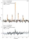 |
Fig. 2 Example of ammonia inversion transition spectra for core #71. Top: NH3 (1,1) spectrum shifted on the y-axis by 1 K. The orange line shows the CLASS hyperfine best fit obtained. Bottom: NH3 (2,2) spectrum. The blue line shows the Gaussian best fit. The best-fit centroid velocity, peak Tmb, FWHM, and S/N are included for both transitions. |
2.3 NH3 map from the GBT KEYSTONE project
The KEYSTONE project used the Green Bank Telescope (GBT) to map 11 GMCs that are part of the Herschel OB Young Stars Survey (HOBYS, Motte et al. 2010) in NH3 and other molecules, using the KFPA receiver and VEGAS spectrometer. The GBT beam has a half power beam width (HPBW) of 32″ at the rest frequency of the NH3 (1,1) transition at 23.694 GHz. We used the available baseline-subtracted NH3 (1,1) and (2,2) data cubes in Sect. 5.2 to investigate the spatial variations of NH3.
3 NH3 data analysis
3.1 Rotational and kinetic temperature
The energy level diagram of NH3 is described by Townes & Schawlow (1975), Ho & Townes (1983) and Rohlfs & Wilson (2004) for example. In the conditions of cold molecular clouds, the so-called metastable states (J, K) = (1,1) and (2,2) can be considered to be coupled only through collisions, and the populations in the upper non-metastable states in each K-ladder can be neglected. Several temperatures can be defined to characterise the state of ammonia molecules.
The rotational temperature describes the populations of metastable levels (J = K) in different K ladders. It is derived from the ratio of lines from different rotation energy levels (the intensity ratio of the inversion transitions in case of NH3). The gas kinetic temperature describes the local velocity distribution of the colliding particles. As dipole transitions between the different K ladders are forbidden, their relative populations depend only on collisions, and measures the gas kinetic temperature (Juvela et al. 2012). With probing the (J, K) = (1,1) and (2,2) lines, we probe only para-NH3 (K ≠ 3, where hydrogen spins are not parallel).
We calculate the rotational temperature of cores that were detected in the (1,1) and (2,2) transitions with the formula given by Ho & Townes (1983) as:
![Mathematical equation: ${T_{{\rm{rot}}}} = {{ - {T_0}} \over {\ln \left\{ {{{ - 0.282} \over {{\tau _{\rm{m}}}\left( {1,1} \right)}}\ln \left[ {1 - {{{T_{{\rm{MB}}}}(2,2)} \over {{T_{{\rm{MB}}}}\left( {1,1} \right)}}\left( {1 - \exp \left[ { - {\tau _{\rm{m}}}\left( {1,1} \right)} \right]} \right)} \right]} \right\}}},$](/articles/aa/full_html/2022/11/aa44000-22/aa44000-22-eq4.png) (1)
(1)
where T0 ≈ 41.5 K is the difference in the energy levels of the two rotational states, τm(1, 1) is the optical depth of the NH3 (1,1) main hyperfine component, and TMB(1, 1) and TMB(2, 2) are the main beam brightness temperatures of the NH3 (1,1) and (2,2) inversion transitions. We get the optical depth of the NH3 (1,1) main hyperfine component from our CLASS fitting, and from the best-fit parameters we can derive the NH3 (1,1) and (2,2) main beam brightness temperatures.
From the estimated Trot, we computed the kinetic temperature using the formula described by Ott et al. (2011) based on large velocity gradient (LVG) modelling assuming optically thin lines (see Ott et al. 2005):
 (2)
(2)
We also computed the kinetic temperature using the semi-empirical formula described by Tafalla et al. (2004):
![Mathematical equation: ${T_{{\rm{kin,T}}}} = {{{T_{{\rm{rot}}}}} \over {1 - {{{T_{{\rm{rot}}}}} \over {41.5K}}\ln \left[ {1 + 1.1\exp \left( {{{ - 16{\rm{K}}} \over {{T_{{\rm{rot}}}}}}} \right)} \right]}}.$](/articles/aa/full_html/2022/11/aa44000-22/aa44000-22-eq6.png) (3)
(3)
A very similar formula was obtained by Bouhafs et al. (2017). Their results agree with ours within 1 K in the Tkin = 1−40 K range, and they suggested the formulas to be used at kinetic temperatures lower than 40 K and volume densities lower than 105 cm−3. We are using both Eqs. (2) and (3) to calculate kinetic temperatures, and we compare the obtained results in Sect. 4.1.
3.2 Excitation temperature, beam filling factor, and volume density
The excitation temperature describes the populations with different J values within a K ladder. This temperature depends on the relative importance of radiative and collisional processes If radiative processes dominate, Tex approaches the value of the background temperature, Tbg. If collisions dominate, Tex approaches the gas kinetic temperature. Therefore, Tex can be well below the rotational and kinetic temperatures if the local thermodynamic equilibrium (LTE) is not reached.
It can be related to the opacity of the main hyperfine component τm through (Ho & Townes 1983):
![Mathematical equation: ${T_{{\rm{ex}}}} = {{{T_{{\rm{MB}}}}\left( {1,1} \right)} \over {\left\{ {1 - \exp \left[ { - {\tau _{\rm{m}}}\left( {1,1} \right)} \right]} \right\} \times \eta }} + {T_{{\rm{bg}}}},$](/articles/aa/full_html/2022/11/aa44000-22/aa44000-22-eq7.png) (4)
(4)
where η is the beam filling factor, and Tbg = 2.73 K is the background temperature. The opacity τm(1, 1) is derived from the spectrum fit (Sect. 2.2). Following Wienen et al. (2018), we assume η = 1, so that this equation provides Tex. As this assumption is done by several studies (e.g. Friesen et al. 2017), it makes it possible to do a fair comparison between them. As we show in Sect. 4.1, this assumption leads to lower limits on the volume densities (see Eq. (5)), because the value η = 1 is an upper limit. In cases where the fit returns the lower bound (0.1) for τm (1, 1), the obtained Tex are not reliable, and we adopt the median value of Tex of the rest of the cores (4.5 K). This is the case for five cores in total.
The local hydrogen volume density can be computed using Eq. (2) of Ho & Townes (1983), assuming that collisions and stimulated emission are balanced against spontaneous emission:
![Mathematical equation: $n\left( {{{\rm{H}}_{\rm{2}}}} \right) = {{{A_{{\rm{ul}}}}} \over C}{{F\left( {{T_{{\rm{ex}}}}} \right) - F\left( {{T_{{\rm{bg}}}}} \right)} \over {F\left( {{T_{{\rm{kin}}}}} \right) - F\left( {{T_{{\rm{ex}}}}} \right)}}\left[ {1 + F\left( {{T_{{\rm{kin}}}}} \right)} \right],$](/articles/aa/full_html/2022/11/aa44000-22/aa44000-22-eq8.png) (5)
(5)
where C is the collisional de-excitation rate (8.5 × 10⁻¹¹ cm3s−1) from Danby et al. (1988), Aul is the spontaneous emission rate (Einstein A coefficient) of the NH3 (1,1) transition (1.7 × 10⁻⁷s−1), and the function F(T) is defined as  , (Harju et al. 1993; Fehér et al. 2016).
3.3 Line width, velocity dispersion, and gas pressure ratio
The line width of the NH3 inversion lines originates from the combination of thermal and non-thermal motions. The thermal line width is related to the kinetic temperature through
 (6)
(6)
where Tkin is the kinetic temperature, k is the Boltzmann constant, and  the mass of the ammonia molecule. The line width relates to the velocity dispersion, σv, as
 (7)
(7)
The non-thermal velocity can be estimated using  where Δv is the line width and Δvth the thermal line width.
From the thermal and non-thermal (or turbulent) line widths we can obtain the ratio of the thermal to non-thermal pressure, that is the gas pressure ratio (e.g. Lada et al. 2003; Urquhart et al. 2015):
 (8)
(8)
3.4 Source-averaged NH3 column density
We estimate the beam-averaged NH3 column density following Rosolowsky et al. (2008) and Friesen et al. (2009), who estimated the NH3 (1,1) column density assuming that the excitation temperature is equal to the rotational temperature:
 (9)
(9)
where ν0 is the frequency of the NH3 (1,1) line, c is the speed of light, Aul is the spontaneous emission rate, g1 and gu are the statistical weights of the lower and upper inversion transition levels, σv is the velocity dispersion, and t is the total optical depth with τ = τm(1, 1) × IJK, where τm(1, 1) is the optical depth of the NH3 (1, 1) main hyperfine line, and is the factor that relates the total optical depth, τ(J, K), to the optical depth of the main hyperfine component, τ(J, K, m), as detailed in Appendix A2. of Mangum et al. (1992):
![Mathematical equation: $\tau \left( {J,K} \right) = \left[ {{{\mathop \sum \limits^{F,F\prime } {{\left( {RI} \right)}_{F,F\prime }}} \mathord{\left/{\vphantom {{\mathop \sum \limits^{F,F\prime } {{\left( {RI} \right)}_{F,F\prime }}} {\mathop \sum \limits^{F,F\prime } }}} \right.\kern-\nulldelimiterspace} {\mathop \sum \limits^{F,F\prime } }}{{\left( {RI} \right)}_{\rm{m}}}} \right]\tau \left( {J,K,m} \right),$](/articles/aa/full_html/2022/11/aa44000-22/aa44000-22-eq16.png) (10)
(10)
where RI is the relative intensity for a quadrupole hyperfine component. For the (1,1) and (2,2) transitions, this can be written as
![Mathematical equation: ${I_{{\rm{J,K}}}} \equiv \left[ {{{\mathop \sum \limits^{F,F\prime } {{\left( {RI} \right)}_{F,F\prime }}} \mathord{\left/{\vphantom {{\mathop \sum \limits^{F,F\prime } {{\left( {RI} \right)}_{F,F\prime }}} {\mathop \sum \limits^{F,F\prime } }}} \right.\kern-\nulldelimiterspace} {\mathop \sum \limits^{F,F\prime } }}{{\left( {RI} \right)}_{\rm{m}}}} \right],$](/articles/aa/full_html/2022/11/aa44000-22/aa44000-22-eq17.png) (11)
(11)
which is equal to 2.000 for (1,1).
A similar method was described by Lu et al. (2014). Their calculations are based on the method presented by Mangum et al. (1992) in their Appendix A2. Assuming that the excitation temperature is equal to the rotational temperature (LTE condition), Lu et al. (2014) compute the column density of the NH3 (1, 1) transition as:
 (12)
(12)
where ν0 is the line frequency in GHz, Δv is the (1,1) line width in km s−1, and τm(1, 1) is the optical depth of the NH3 (1,1) main hyperfine line.
Because of the relatively short lifetime of the non-metastable (J ≠ K) states, all NH3 molecules are assumed to be in metastable states. The total NH3 column density can therefore be obtained by scaling the (1,1) column density as in Friesen et al. (2009):
 (13)
(13)
where Zot is the partition function of the metastable states. Ztot is given as
![Mathematical equation: ${Z_{{\rm{tot}}}} = \sum\limits_J {\left( {2J + 1} \right)S\left( J \right)\exp } {{ - h\left[ {BJ\left( {J + 1} \right) + \left( {C - B} \right){J^2}} \right]} \over {k{T_{{\rm{rot}}}}}},$](/articles/aa/full_html/2022/11/aa44000-22/aa44000-22-eq20.png) (14)
(14)
where S (J) denotes the extra statistical weight of the ortho-over para-NH3 states, with S (J) = 2 for J = 3, 6, 9, and so on, and S (J) = 1 for all other J values, and B and C are rotational constants, 298 117 MHz and 186726 MHz, respectively (Pickett et al. 1998).
When the non-metastable energy levels, J > K, are not populated, Z(J = K) can be given as the sum of the metastable levels (Rohlfs & Wilson 2004). For NH3 in areas of T =10 K and n(H2) ≈ 104 cm−3 this can be written as
 (15)
(15)
Lu et al. (2014) adopted another approximation for the total column density. They adopted the LTE approximation, where the populations of the given molecule are thermalised (Rohlfs & Wilson 2004; Lu et al. 2014), leading to:
 (16)
(16)
where  is the partition function where the rotational constants B and C are given in GHz. According to Lu et al. (2014), this approximation leads to an error of less than 10 % in the range of Trot = 10–50 K.
Table 2 presents the total column density values for each core obtained with the three different methods. For the sake of simplicity, in the rest of the paper we present the results using the method of Friesen et al. (2009) only, and we discuss the systematic differences between the two methods in Sect. 4.1.
Parameters calculated from the NH3 (1,1) and (2,2) with the average, minimum, maximum, and median values of each parameter and their respective standard deviations obtained from the MC calculation.
3.5 Virial parameter
We calculated virial masses and virial parameters based on Bertoldi & McKee (1992), Keown et al. (2017), and Keown et al. (2019). The virial mass is given as
 (17)
(17)
where  is the velocity dispersion of H2 including thermal and non-thermal components, R is the radius of the core, G is the gravitational constant, and
 (18)
(18)
accounts for the radial power-law density profile of the core, where ρ(r) ∝ r−k (Bertoldi & McKee 1992). Similarly to Keown et al. (2019), we assume that the density profile of the cores take the form of ρ(r) ∝ r−1.5, and that the cores are in a steady state, are spherical, and are isothermal.
For the radius R, we used half of the beam deconvolved FWHM size obtained by Motte et al. (2010) from Herschel 160 µm measurements (see Table 1).
The virial parameter is
 (19)
(19)
which is ≲2 for clumps that are gravitationally bound (Rohlfs & Wilson 2004). For Mgas, we used the mass estimates from dust observations (see Table B.1). For the H2 velocity dispersion, we followed the method described in Appendix A.3 of Montillaud et al. (2019) and used the following formula:
 (20)
(20)
where  is the mass of the hydrogen molecule, and the nonthermal velocity dispersion σNT is
 (21)
(21)
where Δv and m are the (1,1) FWHM line width and the mass of the NH3 molecule.
3.6 Uncertainties of the physical properties
To calculate the uncertainties of the physical quantities presented above, one needs to propagate the observational uncertainties through several non-linear equations, potentially leading to complex (non-Gaussian) error distributions. Therefore, we performed Monte Carlo (MC) simulations to derive the uncertainties of the physical quantities from the observational uncertainties and to check the shape of the error distributions. Prior to the MC calculation, the hyperfine structure fit of the NH3 (1,1) line and the Gaussian fit of the NH3 (2,2) line presented in Sect. 2.2 were repeated in Python, using the Scipy curvefit function to obtain the corresponding covariance matrices. We fed them and the errors obtained originally from CLASS to a multi-variate Gaussian random number generator to simulate, for each core, 1000 mock spectra parameters (Tant × τ, vLSR, FWHM(1,1), τm for (1,1); Area, vLSR, FWHM(22) for (2,2)). From these parameters, we derived distributions of core physical parameters: NH3 (1,1) and (2,2) main beam brightness temperatures, kinetic temperatures according to Eq. (2) and (3), column density according to Eq. (13). The standard deviation of the distribution of each parameter was considered as an estimate of its uncertainty. Points with rotational temperature outside the 0−50 K range, or Ntot outside the 0−1017 cm−2 range were deemed non-physical and were excluded from the standard deviation calculation. Figure C.1 shows an example of the observed distributions for core #1. This analysis reveals that although the distributions of Trot and Ntot can be slightly asymmetrical, the standard deviations provide a reasonable estimate of the uncertainties. The standard deviations resulting from the MC are consistent with the errors obtained from the CLASS fitting process.
4 Results
Of the 33 sources observed, we detected the NH3 (1,1) inversion transition towards 31 cores considering an average rms level of TMB = 0.06 K and an average S/N of 12.7.
The NH3 (2,2) transition was detected towards 28 cores, but only 22 cores had a sufficient S/N to carry out the analysis with them. We refer to this sample of 22 cores as the whole sample hereafter. The NH3 (1,1) and (2,2) spectra with the corresponding fit (see Sect. 3.4) are shown in Appendix A, and the best-fit parameters are given in Table B.1 We show the distribution of the obtained parameters in Figs. 3–6, and in Appendices D and F. Table 2 gives the result of all the different physical parameter calculation methods listed in Sect. 3, listing the averages, minima, maxima, and medians.
In the following analysis, we classify our sources into a reliable and a candidate sample based on the S/N of the NH3 (1,1) and (2,2) measurements. The reliable sample consists of 15 cores with both transitions detected, having S/N > 5 for NH3 (1,1) and S/N > 3 for NH3 (2,2). The candidate sample consists of 7 cores with both transitions detected, having 2 < S/N < 3 for (2,2). In the reliable sample, we have seven prestellar and eight protostellar cores. In the candidate sample, we have one warm-starless, one prestellar, and five protostellar cores.
4.1 Core general properties
We discuss here the statistics of our calculations detailed in Sect. 3 considering the physical characterisation of the sample from Motte et al. (2010). This classifies the sample based on the SED into prestellar and protostellar cores, and we discuss their physical properties based on the NH3 observations to search for systematic differences or similarities.
We obtain brightness temperatures, T(11), for the NH3 (1,1) line for the whole sample of between 0.2 and 2.1 K with an average of 0.9 K. For the reliable sample, we obtain values from 0.3 to 2.1 K with an average of 1.1 K, and for the candidate sample values from 0.2 to 0.7 K with an average of 0.5 K. The main hyperfine optical depths, τm(1,1), of the whole sample range from 0.1 to 2.05, and their distribution presents a maximum around 0.1, the lower limit of the line-fitting procedure (see Sect. 2.2). This implies that most of the emission is optically thin; we only find larger (>1.5) values for three protostellar cores, corresponding to 14% of the sample. However, the uncertainties on the optical depth are rather large, between 0.04 and 0.7, peaking between 0.2 and 0.3. Among the 22 sources, four of them have larger errors (0.45, 0.54, 0.63 and 0.68), and the rest of them have errors of between 0.04 and 0.35.
We obtained excitation temperatures for the whole sample of between 3 and 9.13 K with an average of 4.75 K (here we take into account the excitation temperatures replaced by the median excitation temperature of the sample; see Sect. 3.2).
We computed the rotational and kinetic temperatures for the 22 cores where both the NH3 (1,1) and the (2,2) lines were detected. For the whole sample, we obtained rotational temperatures ranging from 10.9 to 23 K, and kinetic temperatures between 11.8 and 24.6 K using the formula of Ott et al. (2011). For the kinetic temperatures, the formula by Tafalla et al. (2004) tends to give larger values than that of Ott et al. (2011), by typically half a degree, which is within the typical uncertainties. Using the formula of Ott et al. (2011), for prestellar sources we obtained kinetic temperatures in the range of 11.8–19.8 K with an average of 15.4 K and a median of 15.5 K. For protostellar sources, kinetic temperatures were between 12.1 and 19.9 K with an average of 15.6 K and a median of 15.2 K.
In Fig. 3, we show the kinetic temperatures obtained from the formula of Ott et al. (2011). We find that the prestellar sources are grouped around 14–16 K, while the protostellar sources are more evenly spread. The KEYSTONE project mapped the RMC in the NH3 (1,1) and (2,2) lines with a median rms of 0.16 K per 0.07 km s−1 channel for both maps (Keown et al. 2019). These authors obtained a median kinetic temperature of 14.2 ± 3.8 K for the area (see Fig. 8 of Keown et al. 2019) and a median velocity dispersion of 0.4 ± 0.1 km s−1. The median kinetic temperatures we obtained for our sources, both prestellar and protostellar are in agreement with this result.
The NH3 (1,1) inversion transitions of the whole sample show line widths between 0.4 and 2 km s−1, well above our velocity resolution of 0.15 km s−1. In Fig. 3a, both the prestellar and the protostellar sources appear to be grouped around Δv1,1= 1 km s−1, with the protostellar sources having a larger spread of values. The NH3 (2,2) line widths range from 0.7 to 2.9 km s−1 (the excluded cores based on their S/Ns have NH3 (2,2) line widths of 4.5 and 5.2 km s−1, with considerably large errors of 0.7 and 0.8 km s−1, respectively; see Table B.1). Figure 4 shows a comparison between the NH3 (1,1) and (2,2) line widths. The sources closer to NGC 2244 are grouped tighter together, while those from AFGL 961, PL03, and PL07 are more aligned to the line indicating equal line widths. Interestingly, the protostellar cores from the Center, Shell, and Extended Ridge have the broadest (2,2) line widths while having average (1,1) line widths. The overall broader line widths obtained for the NH3 (2,2) lines may result from the single Gaussian fitting we used to obtain the line parameters, as it does not take optical depth effects or hyperfine structure into account (Wienen et al. 2012), but may also result from the lower S/N of the (2,2) transition.
The average thermal line width for the whole sample is 0.21 km s−1 with values ranging from 0.18 to 0.26 km s−1. As the measured average line width is 1.1 km s−1, this implies that they are dominated by non-thermal motions.
Using the equations of Friesen et al. (2009), the total NH3 column densities range from 1.1 × 10¹⁴ to 2.3 × 1015 cm−2 with an average of 8.8 × 1014 cm−2 for the whole sample. Two peaks can be seen in the distribution of NH3 column density in Fig. 3 near the obtained minimum and maximum, suggesting two source types. However, we do not find a correlation with the pre- or proto-stellar nature of the sources. The warm-starless source marks the largest value obtained from the whole sample. The NH3 (1,1) column densities calculated from Eqs. (9) and (12) give similar results within typically 8 × 1010 cm−2 to be compared with an average N(1, 1) of 3.3 × 1014 cm−2 (relative difference is less than 1%), while the typical spread in NH3 column densities is 4 × 1014 cm−2 (relative difference is ~30%). This indicates that the differences in the total column density values are due to the different approximations used during the calculation of the partition function (Sect. 3.4).
We used Eq. (4) to calculate Tex and derive  . Our estimates of H2 volume densities are lower limits, because of the assumed beam filling factor of 1 (see Sect. 3.2). The average Tex for the whole sample was 4.75 K and the average volume density 5.6 × 103 cm−3. The range of H2 volume densities is 5.9 × 1022.5 × 104 cm−3. Schneider et al. (2010) estimates the average H2 volume density of clumps over the RMC based on the dust column density map from Herschel. These authors obtain values of between 0.4 and 9.5×103 cm−3, with the highest values found towards the Extended Ridge region of 1.1 × 104 cm−3. These results based on the dust are close to the range of values we find with NH3. As pointed out by Schneider et al. (2010), even our highest H2 volume density estimates are considerably lower than the values predicted by turbulence models of pillar formation of about 107 cm−3 (Gritschneder et al. 2009).
We show the ratio of thermal to non-thermal pressure in Fig. 5. The whole sample has an average Rp of 0.05, suggesting that non-thermal motions are dominant. Core #1, which hosts an evolved protostar, has the lowest Rp followed by the warm-starless core #8. We do not find a significant difference between the prestellar and protostellar populations. Overall, our values are in line with those reported by Urquhart et al. (2015) in a study of 66 massive young stellar objects and compact HII regions of the RMS survey (Red MSX Source survey, Lumsden et al. 2013), where Urquhart et al. (2015) obtained gas pressure ratios Rp =0.01−0.02 for both massive star forming and quiescent clumps. Somewhat higher values of ~0.07 were found by Ragan et al. (2011) who used VLA and GBT NH3 observations towards high-mass star-forming cores, suggesting that the contribution from non-thermal motions may become less important on the smaller, core scales, although the pressure is still dominated by non-thermal motions. This is different from low-mass star-forming cores, where for example towards Barnard 68, based on C18O and C34S data, Lada et al. (2003) obtained an order of magnitude higher values of Rp = 4−5. This indicates that thermal pressure dominates over non-thermal motions. Our sample clearly more closely resembles the samples of massive clumps where non-thermal motions provide a strong contribution to the kinetic energy balance.
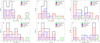 |
Fig. 3 Distributions of the obtained parameters according to the evolutionary stages of the sources covering both the reliable and the candidate sample. The colours represent warm-starless, protostellar, and prestellar cores, and the black outline represents the whole sample, as indicated in the legend. The histograms are (a) NH3 (1,1) line width, (b) NH3 (2,2) line width, (c) NH3 (1,1) main hyperfine component optical depth – all of which are from CLASS fitting (see Sect. 2.2) –, (d) thermal line width calculated from Eq. (6), (e) kinetic temperature calculated from Eq. (2), and (f) NH3 column density calculated from Eq. (13). |
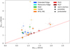 |
Fig. 4 NH3 (1,1) and (2,2) line widths with their errors. The red line marks equal widths. The warm-starless, prestellar, and protostellar cores are indicated with squares, circles, and stars, respectively. The colours represent the areas where the cores are from (see Fig. 1). The filled points mark the reliable sample, the open points the candidate sample. The point that has a (2,2) FWHM of 5.15 km s−1 has been excluded from further analysis based on its broad line width. |
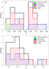 |
Fig. 5 Distribution of the (a) gas pressure ratios and (b) virial parameters. The low gas pressure ratio of the warm-starless core #8 may suggest a more turbulent line width for these types of cores. However, this core is not depicted in the bottom panel because of its significantly higher α of 12.32. |
4.2 Virial analysis
We show the distribution of virial parameters (see Sect. 3.5) in Fig. 5. Core #8, the single warm-starless source is an outlier with a significantly higher α of 10.84, which is not shown here. We find that the virial parameter for the whole sample is between 0.3 and 2.6, with an average of 1.1. A source can be considered as gravitationally unstable when α ≪ 2 (Bertoldi & McKee 1992; Kauffmann et al. 2013); nine cores of our sample have α < 1 and four have α ~ 1. This suggest that most of the clumps are likely to be gravitationally unstable and undergo collapse. This also includes Core #1, which was highlighted by Motte et al. (2010) as one of the high-mass, high-luminosity cores and a possible precursor to an OB type star. With an α of 1.78, our results are in agreement with this clump being potentially gravitationally unstable. We find the highest values of α ~ 2 for core # 36, which is located in the Extended Ridge and has been characterised as prestellar. However, our virial parameter estimates suggest that it is close to being gravitationally stable, and could therefore be a starless condensation. However, there are some caveats when estimating the α parameter, such as that the NH3 observations may not trace the same volume of gas corresponding to the dust-based mass estimates, although the difference in the beam sizes is rather small. We compare the NH3 measurements taken in the 40″ Effelsberg beam with the Berschel observations smoothed to ~37″, corresponding to the resolution of the 500 µm map. More importantly, these estimates do not take into account the effect of the magnetic field that may play a role in the stabilisation of the clumps (e.g. Zhang et al. 2014; Wareing et al. 2018).
Within the frame of the KEYSTONE project, Keown et al. (2019) also carried out a study of the virial parameter based on a dendrogram analysis of their NH3 maps and dust observations from Berschel. Using the same formulation as that used here, and considering dendrogram leaves covering typically larger areas, these authors estimate a range of α values of ~0.3−20. Our distribution of values corresponds to the lower end of these values. This is expected because, in the KEYSTONE project, the sources are defined as the dendrogram leaves in a large map, which may include relatively low-density sources, while in our study the sample selection was based on a preselection of compact sources designed to identify prestellar and protostellar cores. They also cross-matched their 48 dendrogram leaves identified towards Rosette with YSO catalogues, which revealed a similar fraction of about 42−46% of the leaves associated with protostars and gravitationally bound as suggested by the virial analysis. While the overall range of α values is similar to that found by Keown et al. (2019), we have a significantly larger fraction of ~90% of gravitationally bound cores with α < 2. The fact that our sample tends to show a larger fraction of gravitationally bound clumps could be due to the source selection and the smaller area considered here. While we compute the virial parameter over a radius of 0.05−0.25 pc, their effective radius is about 0.1−0.4 pc.
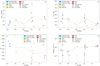 |
Fig. 6 (a) NH3 (1,1) line width, (b) kinetic temperature, (c) gas pressure ratio, and (d) column density plotted against the projected distance of the cores from NGC 2244. The filled points mark the reliable sample, the open points the candidate sample. The black and the grey lines indicate a running median of the values using non-uniform binning for the reliable and for the whole sample, respectively. The distances are shown in degrees with 1° corresponding to 28 pc at a distance of 1.6 kpc. |
5 Discussion
5.1 Overview of the region
In this section, we put our results in perspective with the regions outlined by Schneider et al. (2010) and the clusters described by Phelps & Lada (1997) and Román-Zúñiga et al. (2008) with a particular focus on the spatial variation of our NH3 results across the RMC. Figure 6 indicates how the different parameters vary with the increasing projected distance (assuming that all objects are in the same plane on the sky) from the OB cluster, NGC 2244 by showing the running median (RM) of the parameters. Our observed positions lie within a projected distance of 1.4 degrees of NGC 2244 which corresponds to a maximum projected separation of ~40 pc at a distance of 1.6 kpc.
The southern part of the arc around NGC 2244 related to the extended PDR, the so-called Shell region, contains the cluster PL01 (see Fig. 1). We have two sources from the reliable sample here: a protostellar core associated with PL01, and a prestellar core outside of PL01. This prestellar source, core #39, has the highest gas pressure ratio of the whole sample, suggesting a strong contribution from external pressure or compression contributing to the observed line widths.
The Monoceros Ridge is an area of gas compression at the cloud-nebula interface (Román-Zúñiga & Lada 2008) with the cluster PL02 towards the Extended Ridge. This latter part is more exposed to the ionising radiation of NGC 2244, and therefore has strong temperature and density gradients (Schneider et al. 2010). Three sources from our reliable sample, two prestellar and one protostellar, fall into the Extended Ridge along with a candidate protostellar source. Two candidate sources, one prestellar and one protostellar, are in the Monoceros Ridge. There are slight decreases in temperature and column density when comparing these regions in the running medians of Figs. 6b and 6d, although the large uncertainties, especially in NH3 column densities, prevents us from drawing firm conclusions.
The cluster PL03 lies about 20−30 pc away from NGC 2244 in a gas clump outside the main area of the cloud. Two candidate sources, the warm-starless core #8 and a protostellar core, fall into this area, with one reliable protostellar source. The warm-starless core #8 marks the maxima in the kinetic temperature and NH3 column density plots of Fig. 6. Its gas pressure ratio is among the lowest, implying dominant non-thermal motions in the core. However, these values have large uncertainties due to the relatively low S/N of the source (4.3 for TMB(1, 1) and 2.65 for TMB(2, 2)).
The Center area, including PL04, PL05, and REFL08, was reported to be in direct interaction with the shock front from NGC 2244 by Heyer et al. (2006). These three clusters make up almost 50% of the total embedded YSO population of the cloud (Román-Zúñiga & Lada 2008). For the cores in this area, we had a high non-detection rate (five cores with no line detections or insufficient S/N). This is rather unexpected given the large dust column densities revealed by Herschel, although the spatial distribution of the NH3 emission from Keown et al. (2019) indeed shows a highly non-homogeneous distribution for NH3. However, the three detections – two candidate protostellar and one reliable protostellar source – have lower kinetic temperatures than and similar column densities to the other cores of the Ridges and the Shell, where the interaction between the molecular medium and NGC 2244 is more evident. The study of Keown et al. (2019) shows NH3 (1, 1) and (2, 2) detections in the area of REFL08, but not in PL04 or PL05. In contrast with the conclusions of Heyer et al. (2006), the low Tkin and N(NH3) values obtained together with the non-homogeneous NH3 distribution suggest a less pronounced interaction with the shock front from the nebula. In all panels of Fig. 6, the cores from this area mark a break in the RM.
Associated with cluster PL06 is a B-type binary protostellar system, AFGL961 (Román-Zúñiga et al. 2008). According to NIR observations, PL06 includes around 30 young sources, of which at least 9 are associated with shock-like features (Aspin 1998). In this area, we have four prestellar sources and one protostellar source, all in the reliable sample. These sources have high NH3 column densities compared to the Ridges and the Shell, all about 1015 cm−2. However, the rest of their parameters obtained from NH3 exhibit the largest dispersion in this region. This could be a statistical effect because this area has the greatest number of sources in our sample.
The cluster PL07 is surrounded by compact gas emission forming an envelope around the cluster, similarly to PL01 and PL06. Román-Zúñiga et al. (2008) claim that triggered star formation is unlikely in this area because of its distance from the shock front as it lies in a region beyond the main interaction with the cluster. In PL07, we have three reliable protostellar sources. They all have similar temperature and column density parameters, but a wider range of gas pressure ratios. Core #18 has higher αvir and H2 volume density than the two other sources. Altogether, high NH3 column densities and low kinetic temperatures characterise our sources associated with this region.
Using dust emission from Herschel data, Schneider et al. (2010) noted the gradient in average H2 volume density from the ‘compression’ zone towards the more distant areas, ranging from 0.5 × 103 cm−3 (Shell, Extended Ridge, and Monoceros Ridge) to 3.9 × 103 cm−3 (PL07). We also note a global increase in the total NH3 column densities and a slight increase in the RM of the NH3 (1, 1) line widths with the distance where the spread of the values gets larger until the RM drops for the three sources of PL07. Overall, the RM of kinetic temperatures shows a decreasing trend with increasing distance from NGC 2244, except for the sources in AFGL 961 which might be dominated by local heating due to the high density of protostellar sources. This overall trend seems consistent with the idea that the heating by NGC 2244 decreases with distance, and broadly corresponds to the increase in the aforementioned volume and column densities. The gas pressure ratios also show a decrease, although the spread of the values is considerable.
5.2 Dust and NH3 spatial variations
In order to investigate the spatial variation between the thermal dust emission and NH3 emission, we complemented our data from the publicly available maps of the KEYSTONE project (Keown et al. 2019). This complements our more sensitive Effelsberg data set, which is composed of pointed observations, and allows us to investigate the spatial variations in ammonia emission. Figure 7 shows their NH3 (1,1) integrated emission for the whole Rosette region and close-up views of the main regions discussed above. The comparison with the thermal dust emission traced by the Herschel 250 µm shows that the NH3 emission is typically more compact than the dust. This is consistent with the NH3 tracing relatively dense gas.
While we do not see significant NH3 emission without thermal dust, interestingly, many sources exhibit a shift between the ammonia and the dust emission peak. This is particularly striking in the Extended Ridge region, where Fig. 7 shows that dust emission tends to peak northwest of the ammonia peak. A practical consequence of this is that the coordinates of some of our Effelsberg pointed observations are somewhat shifted from the ammonia peak, because the targets were selected from Herschel maps, well before the Keown et al. (2019) study. This suggests that for targets with a large shift, the physical properties derived from our pointed observations may not be representative of the source properties, with a plausible bias towards lower column and volume densities and higher temperature. It can also be noted that in the Center region, our observations do not sample the most intense emission in the southern part of this region.
We quantified the shift between the NH3 and dust emission peaks by visually examining the Herschel 250 µm and the integrated ammonia maps from Keown et al. (2019) for the observed Effelsberg positions covered by the GBT map. Figure 8 summarises the observed shifts for all the sources where an emission peak could be observed for both the dust and ammonia. This approach is biased in the sense that sources located within the densest regions of the cloud are affected by significant confusion, and a clear maximum for at least one tracer was difficult to identify. The typical uncertainty in the shift amplitude comes from the limited resolution of the maps. The pixel sizes are 6″ and 9″ in the Herschel and ammonia maps, respectively, leading to a typical uncertainty of 10–15″ (for quadratic or simple combination, respectively). We measure shifts in Fig. 8 of the order of 10″ to 20″. These can be considered consistent with the intrinsic position error measurements and seem compatible with simple statistical dispersion. However, when focusing on the Extended Ridge region, the average shift is approximately 18″ with an uncertainty reduced to 5 to 8″ if one assumes independent errors and therefore divides the uncertainty by the square root of the number of points. A systematic shift may also arise from pointing errors from the observations, and this could possibly explain the overall shift to positive Δδ values (only five sources have Δδ < 0, while 17 have Δδ < 0). Considering both the measurement and observational uncertainties, it remains notable that sources in the Extended Ridge, Monoceros Ridge, and the isolated easternmost source of the Center region consistently present an approximately 20″ shift towards the west or northwest, the approximate direction of the NGC 2244 open cluster. In Fig. 7, the close-up view of these regions shows that dust emission contours closely follow the brightest ammonia sources, while in the same view the dust-to-ammonia shift is visually clear for several sources, especially the isolated ones. This seems incompatible with the systematic shift expected for a pointing error. Overall, the data suggest that a genuine shift exists between the dust and ammonia emission for the isolated sources in the Extended and Monoceros ridges.
Harju et al. (2020) reported asymmetric distributions of molecules in the starless molecular cloud core Ophiuchus/H-MM1 that have been interpreted as a combination of photodissociation on the irradiated side and shading effect on the opposite side. Due to the irradiation of the nearby cluster, a similar phenomenon may explain the shift of the NH3 and the dust emission towards the Extended Ridge regions. Observations of higher angular resolution would be necessary to investigate whether similar effects are seen towards our targets.
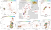 |
Fig. 7 Integrated NH3 intensity from Keown et al. (2019) in K km s−1. The red contours show the Herschel dust emission at 250 µm. In the central map, the grey area indicates the zone not covered by Keown et al. (2019) observations, and the contour is at level 400 MJy sr−1. In the close up views of the region, the contours are at levels of 400, 500, and 600 MJy sr−1 for the Monoceros Ridge and the Extended Ridge; at 400, 500, 1000, and 1500 MJy sr−1 for PL03; at 400, 500, 1000, and 2000 MJy sr−1 for the Shell; at 400, 500, 1000, 2000, and 4000 MJy sr−1 for AFGL 961; and at 600, 800, 1000, 1200, and 1400 MJy sr−1 for the Center. The open squares show the Effelsberg targets with the same colour code as in Fig. 1. |
5.3 Correlations
Here, we examine the correlations between the various physical parameters we obtained from our NH3 analysis in Fig. 9 and Appendix D. In Fig. 9, most sources show the classical anti-correlation between kinetic temperature and ammonia column density, although three of the densest sources, which also present the largest uncertainties, depart from this trend with large kinetic temperatures. Two of these outliers are protostellar sources, which may explain their high temperatures. The third one is the peculiar warm starless core #8 (discussed in Sect. 5.5).
We also examined correlations between NH3 and dust parameters. As presented in Sect. 5.1, Motte et al. (2010) and Schneider et al. (2010) examined the properties of the RMC based on Herschel observations, obtaining a physical size (from a 2D Gaussian fit to the 160 µm image after subtracting a >0.5 pc background), dust temperature, bolometric luminosity, and mass estimates (from SED analysis assuming optically thin 350 µm emission) for the cores, which are summarised in Table 1. Figure 10 and Appendix F show the relation between the physical parameters obtained from NH3 and dust.
Figure 10 shows the dust temperature, the NH3 (1,1) and (2,2) line widths, gas pressure ratios, main hyperfine optical depth, kinetic temperature, and NH3 column density, and we computed the Pearson r correlation coefficient and p-value. For the reliable sample, we find high Pearson r coefficients for the correlation between the dust temperature and the NH3 (1,1) line widths (Fig. 10a), with r = 0.83 and a p-value <0.00 (r = 0.84 and p-value <0.01 for the whole sample). For the correlation between the dust temperature and the NH3 (2,2) line widths (Fig. 10c), we find r = 0.73 and a p-value < 0.00 (r = 0.54 and p-value <0.01 for the whole sample). Correlating the dust temperature and the kinetic temperature (Fig. 10d) provides r = 0.67 and a p-value of 0.01 (r = 0.72 and p-value <0.01 for the whole sample) suggesting a positive correlation between these parameters. The gas pressure ratio and the dust temperature on Fig.10e show a possible anticorrelation with r = −0.49 and a p-value of 0.06 (r = −0.51 and a p-value of 0.02 for the whole sample); however, cores with a lower dust temperature show a high scatter in Rp and the trend may be mostly due to the two high Tdust sources. In the rest of the figures (Figs. 10b, f), the points are very scattered revealing a flat or statistically unreliable trend with high p-values. Figure 10f, which depicts dust temperatures and NH3 column densities, shows a flat trend, with many cores showing low column densities, and the warm-starless core #8 and another protostellar core showing bigger column densities along with higher dust temperatures.
5.4 Star formation properties
The impact of the NGC 2244 cluster on the star formation in the RMC and the question of triggered star formation in this region have long been under discussion. Schneider et al. (2010) found an age gradient in an increasing ratio of prestellar and young protostellar cores to more evolved protostellar cores with increasing distance to the cluster NGC 2244, implying that star formation in Rosette is probably influenced by the radiative impact of the cluster. Cambrésy et al. (2013) estimated the age distribution of YSO clusters with WISE photometry in Rosette and found that the evolution of the complex is not influenced by its OB star population. Their analysis supported the conclusion of Heyer et al. (2006), who found that the expansion of the gas ionised by the OB stars has only spatially limited effects and does not have a significant impact on the global dynamics of the cloud. Similarly, from morphological and probability density function analysis, Schneider et al. (2012) found that star formation in Rosette is not globally triggered by the impact of UV radiation. These authors concluded that star formation occurs at its filaments, which originate from the primordial turbulent structure built up during the formation of the cloud where the column density is high enough, and also in the Shell region, where we can observe the compression of gas. However, local triggering may still be possible. Román-Zúñiga & Lada (2008) claim that the apparent age sequence of the clusters indeed indicates a sequential star formation in time, but that the relative age differences are not large enough to account for the triggered cluster formation scenario of Elmegreen (1998). Román-Zúñiga & Lada (2008) therefore propose a primordial overall age sequence. Wareing et al. (2018) were able to reproduce the structure of the region with a mechanical stellar feedback model using a thin sheet-like molecular cloud. These authors suggest a possibility for localised triggered star formation for the southeast side of the nebula along the direction where they have imposed magnetic field in their model.
As discussed in Sect. 5.1, we find no clear evidence for triggered star formation at a global scale. To see if there is an effect of local triggering, we used the 7 O- and 24 B-type stars that NGC 2244 hosts and the AllWISE YSO candidate catalogue (Marton et al. 2016). We calculated the angular distance between the cores and YSO candidates and O and B stars, before selecting the smallest distance between each core and YSO or OB star, and making correlation plots using those values. Figure E.1 shows the variations of Tkin and N(NH3) with the distance to the Class I/II, Class III, and O/B stars. The spread in Tkin and N(NH3) tends to decrease with the distance to Class I/II YSOs. We do not see any strong trends in the parameters with the projected distances in either of the figures as we find both high and low kinetic temperature and column density values in the vicinity of all types of YSOs and OB type stars. Figure E.2 shows strong scatter in Tdust (from 12 to 37 K) in the first ~0.6 pc around Class I/II protostars, and relatively little scatter (from 14 to 16 K) beyond this distance. The situation is less clear around Class III objects. These variations in Tdust suggest that the more actively star-forming clumps, where Class I/II protostars are found, tend to have more complex and contrasted substructures. Examples of such substructures were reported, for example in Monoceros OB1 (Montillaud et al. 2019), where a clump hosts several cores, including both a warm core harbouring a Class I/II protostar and a cold starless core. However, higher resolution data would be needed to conclude whether local triggering is playing a role here.
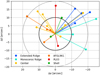 |
Fig. 8 Spatial shift between the NH3 and dust maxima for targets where both KEYSTONE and Herschel data are available. For the missing sources, no maxima are visible for at least one dataset. The colours show the region hosting the source as mentioned in the legend. The shift of Δα = −18″, Δδ = 13″ corresponds to the isolated source east of the Center region. The circles have 10″ and 20″ radii, corresponding to 25% and 50% of the Effelsberg beam size, and to 31% and 62% of the GBT beam size. |
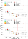 |
Fig. 9 NH3 column density and kinetic temperature. The symbols and colours are as in Fig. 4. The grey line indicates a linear fit for the whole sample, the black line for the reliable sample. The Pearson correlation coefficients are noted with the same colours. Bottom: The red square indicates three outlier sources, which have been excluded from the correlation measurements in this panel. |
5.5 Core #8
The warm-starless core #8 is the most peculiar object in our sample, with the highest ammonia column density but the lowest hydrogen volume density, the highest kinetic temperature, the largest virial parameter, and the second lowest gas pressure ratio after core #1, a reliable protostellar source in AFGL961. The α parameter and the rest of the parameters point towards a gravitationally unbound object. On the other hand, the α value does not account for external pressure, while the low gas-pressure ratio indicates large non-thermal motions. If these motions correspond to longitudinal motions rather than solenoidal ones, as in converging flows for example, external pressure would play a significant role in the source boundedness. Figure 7 shows that core #8 is at the centre of the PL03 protocluster as traced by dust emission, but that it is away from the dense gas structure seen in ammonia in the western part of PL03. Unfortunately, the sensitivity of the KEYSTONE data is too limited to reveal ammonia emission across PL03 and, therefore, to examine possible velocity gradients in the dense gas that might support the idea that core #8 is formed by dynamical pressure. Our data are more sensitive but are limited to the discrete locations of the four PL03 cores: #76 on the northeast, #8 and #16 near the centre, and #5 in the western part of PL03. They show a difference in radial velocities of about 1 km s−1 from core #76 to core #5, and only of ~0.5km s−1 from the two central cores to core #5. Thus, unless the gas flows mainly parallel to the plane of the sky, it seems unlikely that the warm starless core #8 is bound by external pressure, and it is more likely to be a transient structure.
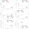 |
Fig. 10 NH3 (1,1) and (2,2) line width, gas pressure ratio, (1,1) main hyperfine component optical depth, kinetic temperature, and column density plotted against dust temperature. The filled points mark the reliable sample, the open points the candidate sample. The grey line indicates a linear fit for the two parameters for the whole sample, the black line for the reliable sample. The Pearson correlation coefficients are noted with the same colours. The rest of the correlation plots for ammonia and dust parameters are included in Appendices F.1, F.2, and F.3. |
5.6 Rosette, an intermediate-mass star-forming region
We compared our results with parameters obtained from studies of different star-forming regions. To this end, we selected surveys using NH3 data as well as studies on high- and low-mass star-forming regions. For high-mass star-forming regions, we used the ATLASGAL star-forming clumps from Wienen et al. (2012), and the star-forming clumps of G333 from Lowe et al. (2014). For low-mass star-forming regions, we selected the dense core candidates in Perseus from Rosolowsky et al. (2008), and the dense cores in Ophiuchus from Friesen et al. (2009). We used both of our samples in the comparison, that is, the reliable and the candidate sample.
The ATLASGAL sample from Wienen et al. (2012) covers high-mass star-forming clumps at various evolutionary stages in the inner Galactic disc over a large range of distances. These sources are more extended than our compact cores. The highmass star-forming region examined by Lowe et al. (2014), G333, is a giant molecular cloud (GMC) of the southern Galactic plane associated with the HII region RCW 106 (Rodgers et al. 1960), at a distance of 3.6 kpc. This is the fourth-most active star-forming region in the Galaxy (Urquhart et al. 2014) containing bright HII regions and high-mass star-forming clumps. Their sample contained 20 IR-bright and 26 IR-faint objects.
For the comparison of our sample to low-mass star-forming regions, we selected dense core candidates in Perseus at a distance of 260 pc from Rosolowsky et al. (2008). These latter authors detected NH3 towards 162 cores. We also compared our sample to that of Friesen et al. (2009), who analysed the initial conditions of clustered star formation in Ophiuchus at 120 pc. These latter authors selected three areas: Oph B, C, and F, finding 14, 3, and 3 sources, respectively.
To calculate kinetic temperatures from NH3, Friesen et al. (2009) and Wienen et al. (2012) used the method of Tafalla et al. (2004), which we used as well and outline in Sect. 3.1. Rosolowsky et al. (2008) and Lowe et al. (2014) used the method of Swift et al. (2005). In this method, assuming that Tkin < T0 ≈ 41.5 K, which implies that only the (1,1) and (2,2) states are populated, the relationship between the rotational and kinetic temperature is
![Mathematical equation: ${T_{{\rm{rot}}}} = {{{T_{{\rm{kin}}}}} \over {1 + {{{T_{{\rm{kin}}}}} \over {{T_0}}}\ln \left[ {1 + 0.6\exp \left( {{{ - 15.7} \over {{T_{{\rm{kin}}}}}}} \right)} \right]}}.$](/articles/aa/full_html/2022/11/aa44000-22/aa44000-22-eq32.png) (22)
(22)
As detailed in Sect. 3.1, we calculated kinetic temperatures following the method of Tafalla et al. (2004) and Ott et al. (2011). Of the three methods, the results of Ott et al. (2011) give the lowest values on average. The results obtained following the method of Swift et al. (2005) differ from the results obtained following the method of Ott et al. (2011) in an average of 1, returning both lower and higher values. The method of Tafalla et al. (2004) gives the highest values on average for a given dataset. The method for calculating kinetic temperature for each sample is noted in Fig. 11. For our sample, the averages are Tkin,O = 15.92 K, Tkin,S = 16.93 K, and Tkin,T = 17.98 K.
To obtain NH3 column densities, the methods used for the other samples give similar results. To calculate N(1,1), Eq. (4) in Lowe et al. (2014), Eq. (5) in Wienen et al. (2012), and Eq. (A4) in Friesen et al. (2009) give similar results. Equation (13) in Rosolowsky et al. (2008) gives a lower value (~51−53% of what the other equations give as a result) because it does not include both parity states of the NH3 (1,1) level in the (1,1) column density (as stated in Friesen et al. 2009). To calculate total NH3 column density, Eq. (5) of Lowe et al. (2014) and Eq. (4) of Wienen et al. (2012) use the same approximation, while Rosolowsky et al. (2008) and Friesen et al. (2009) use another approximation. All approximations give similar results, except for that of Rosolowsky et al. (2008) because of the aforementioned limitation of their (1, 1) column density calculation.
The ATLASGAL sample has an average kinetic temperature of 20 K (13−40 K), and an average NH3 column density of 2 × 1015 cm−2, corresponding to warmer and denser gas compared to ours. This sample of Galactic star-forming regions shows masses of 60−104 M⊙ and exhibits broad line widths. The sources of the ATLASGAL sample that have broad line widths have virial parameters that imply that they are supported against gravitational collapse. They obtain lower virial parameters for sources with narrow line widths. Our sample shows a variety of cores that are in virial equilibrium and are gravitationally unstable but we have to note the uncertainties of our calculations.
For the sources of G333, the IR-bright sample had on average higher kinetic temperatures around 24 K and had NH3 column densities around 1016 cm−2, while the IR-faint cores had lower kinetic temperatures around 19 K and similar column densities. Both of these samples are warmer and have significantly higher column densities on average than ours. In the column density calculation for the G333 sample, Lowe et al. (2014) were also assuming the same excitation temperatures for all hyperfine lines and homogeneous excitation conditions along the beam and used the derivation of Mangum et al. (1992) and Li et al. (2003). Lowe et al. (2014) found that the clumps cluster into three regions, and based on the clustering of the IR-bright clumps into the centre of each region, they concluded a possibility of sequentially triggered star formation as their parameters indicated a different evolutionary status for the IR-faint clumps, which were clustering towards the edges of each region. In our sample of prestellar and protostellar cores, we do not see any significant clustering of positions or parameters similar to that of the IR-faint and IR-bright clumps in the sample of Li et al. (2003), which otherwise would suggest a global triggering effect.
The dense core candidates in Perseus had line widths of between 0.08 and 0.7 km s−1 with an average of 0.2 km s−1, which are well below our average of 1.1 km s−1. Their cores have an average kinetic temperature of ~11 K, which is than the average of our sample of 16.2K. We obtained a maximum kinetic temperature of 24.6K, while the warmest core from Rosolowsky et al. (2008) is 26 K. However, precaution must be taken with these values, because the beam coverage of nearby low-mass star-forming regions does not necessarily cover the same structures our beam coverage did. Regions of low column density found for the dense cores by Rosolowsky et al. (2008) have similar values to those of our sample (5.04 × 1013 cm−2−2.29 × 1015 cm−2).
In Ophiuchus, the Oph C area was the coldest with an average kinetic temperature of 12 K and (1,1) line widths of between 0.1 and 0.7 km s−1. Also, its NH3 column densities of around 5.3 × 1014 cm−2 and its H2 volume densities of 0.8−4.2 × 104 cm−3 fall into the range of our obtained values. Oph B had a wider range of (1,1) line widths, an average of 0.8 km s−1, an average kinetic temperature of 15 K, an NH3 column density of 4.6 × 1014 cm−2, and a volume density of 5.9 × 104 cm−3. Oph F is similarly warm but less dense in both column and volume densities.
Figure 11a shows the kinetic temperatures and the NH3 column densities of all the compared samples. For NH3 column density, our sample falls between the parameters of the Perseus and the ATLASGAL sample. The high-mass cores of G333 have the highest NH3 column densities; the low-mass cores of Perseus have the lowest, but they cover a wide range of column densities.
We calculated gas pressure ratios for all samples as detailed in Sect. 3.3. In Figs. 11b, c, we can see the distribution of gas pressure ratios with kinetic temperatures and NH3 column densities. The high-mass cores of G333 and the ATLASGAL sample have the lowest gas pressure ratios. With the exception of the few high gas-pressure ratios of Perseus, all of the cores seem to be dominated by non-thermal motions.
Altogether, our sample is warmer and exhibits higher NH3 column densities than other nearby low-mass star-forming regions, while it is colder and has lower NH3 column densities than high-mass star-forming regions. Our sample is considerably less dense than the clumps of the high-mass star-forming GMC.
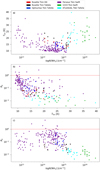 |
Fig. 11 Comparison of the parameters of our sample of cores with those of different star-forming regions. (a) Kinetic temperatures and NH3 column densities, (b) kinetic temperatures and gas pressure ratios, and (c) NH3 column densities and gas pressure ratios of our sample of cores from the Rosette Molecular Cloud along with the samples from Perseus of Rosolowsky et al. (2008), from Ophiuchus of Friesen et al. (2009), from the ATLASGAL survey of Wienen et al. (2012), and from G333 of Lowe et al. (2014). The samples of Perseus and Ophiuchus show the widest range of gas pressure ratios. The red dashed line marks Rp = 1. In (c), the red and black points of Rosette overlap as the figure does not depict kinetic temperatures. The column densities of Rosolowsky et al. (2008) have lower values, ~51−53% of what the other equations used by the other samples give as a result. |
6 Summary
The Rosette molecular cloud is one of the template regions the detailed study of which contributes to our understanding of massive star formation. To contribute to characterising this region, we selected 33 dense cores from Herschel dust emission maps. We observed these with the Effelsberg 100-m telescope in the (1,1) and (2,2) NH3 inversion transitions in single pointing mode, providing deep (rms ~ 60 mK in TMB) ammonia spectra capable of detecting the dense gas ( ~ 104 cm−3) in these objects. We detected the NH3 (1,1) and (2,2) inversion transitions in 31 and 28 targets, respectively, leading to a reliable sample of 15 sources and a candidate sample of 7 sources. We investigated the physical properties of these sources and put them in perspective with the present understanding of the nature and evolution of the Rosette molecular cloud. We reached the following conclusions:
We obtained kinetic temperatures and NH3 column densities with different methods. The methods for calculating the NH3 (1,1) column density agree very closely, but the methods for obtaining the total NH3 column density result in more significant differences, that is, differences of 4 × 1014 cm−2 on average. Assumptions on LTE and the use of different temperature values (rotational or excitation temperature) can account for some of these differences;
We observed line widths in the range of 0.4−2 km s−1, dominated by non-thermal motions. The kinetic temperatures derived from ammonia are mostly between 12 and 20 K, and the ammonia column densities are within the 1014−2 × 1015 cm−2 range;
For most sources, the virial parameter α was found to be smaller than the threshold of 2 for gravitational collapse. However, the large uncertainties in this method make it difficult to disentangle a core in virial equilibrium from a collapsing core or an unbound core. A notable exception was found for the warm starless core #8 whose large value indicates it is very likely an unbound structure;
The spatial variations of kinetic temperature and ammonia column density with distance to the open cluster NGC 2244 show large scatter. This is compatible with the idea that temperature decreases and column density increases with distance from NGC 2244 on the condition that the sources from the dense protocluster AFGL 961 are discarded from the trend. This view is consistent with the idea that the cluster has an impact − probably through its radiation field – on the evolution of the cloud, except in the densest regions the evolution of which is fully driven by their internal characteristics;
This latter view is possibly supported by the tentative detection of a shift between the locations of ammonia and dust emission peaks. Higher resolution data are necessary to assess this possibility;
We find no additional evidence for globally triggered star formation. However, our findings can support the scenario of locally triggered star formation and the influence of the primordial structure of the cloud on its star formation processes;
Overall, the gas parameters of the cores fall between those of the low- and the high-mass star-forming regions. We did not obtain column densities as large as that found in one of the most active high-mass star-forming regions. The lower limit for our H2 volume density estimates falls within the range of H2 volume densities of low-mass star-forming regions.
Acknowledgements
Based on observations with the 100-m telescope of the MPIfR (Max-Planck-Institut für Radioastronomie) at Effelsberg. Herschel is an ESA space observatory with science instruments provided by European-led Principal Investigator consortia and with important participation from NASA. This research was made with the support of the Erasmus+ programme of the European Union, the Hungarian OTKA grant NN111016, the Balaton program 40470VL and the TÉT grant 2017-2.2.5-TÉT-FR-2017-00027. This research was partially supported by the TKP2020-NKA-04 DE-SPACE project. R.B acknowledges support from the French Institute of Hungary, the Carnot-Pasteur Doctoral School of Université de Franche-Comté, and the Physics Doctoral School of Eötvös Loránd University. T.Cs. acknowledges support from the Deutsche Forschungsgemeinschaft, DFG via the SPP (priority programme) 1573 ‘Physics of the ISM’. N.S. acknowledges support through the project “GENESIS” (ANR-16-CE92-0035-01/DFG1591/2-1), the DFG project number SFB 956, and from the BMWI via DLR, project number 50 OR 1916 (FEEDBACK).
Appendix A Fit results
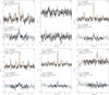 |
Fig. A.1 Ammonia spectra for cores #1 to #5 and #7, as indicated in the top-right corner of each frame. In each panel, the top spectrum is the NH3 (1,1) spectrum shifted by 1 K. The orange line shows the CLASS hyperfine best fit obtained. The bottom spectrum is NH3 (2,2) spectrum. The blue line shows the Gaussian best fit. The best-fit centroid velocity, peak Tmb, FWHM, and S/N are included for both transitions. The grey parts of the spectra were outside the analysed velocity range, which were defined around the vIsr(1,1) and vIsr(2,2) values. |
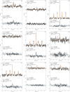 |
Fig. A.1 continued for cores #8 to #13 and #15 to #17. |
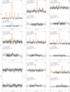 |
Fig. A.1 continued for cores #18 to #20, #22, #24, #28, #31, #36, and #39. |
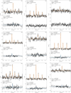 |
Fig. A.1 continued for cores #41, #43, #45, #46, #49, #50, #52, #71, and #76. |
Appendix B NH3 (1,1) and (2,2) fit parameters
Parameters obtained from the NH3 observations.
Appendix C Example result of the Monte Carlo simulations
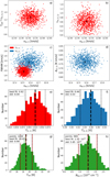 |
Fig. C.1 Results of the MC simulations for core #1. Frames (a), (b), and (c) show parameters obtained for the NH3 (1,1) line, (c) and (d) for the (2,2) line. Frame (e) shows the distribution obtained for (1,1) temperature, (f) for (2,2), (g) for rotational temperature, and (h) for NH3 column density. Black crosses show the values obtained from the CLASS fitting. The red dashed lines indicate the 16, 50, and 84 percentiles, the thin black dashed lines show the standard deviation, and the thick black dashed line shows the values obtained with the best-fit parameter. |
Appendix D NH3 correlation plots
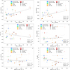 |
Fig. D.1 Correlation plots between different parameters calculated from the ammonia data. |
Appendix E Projected distance plots
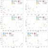 |
Fig. E.1 Distance of the cores from the closest Class I/II (top row) or Class III YSO candidate (middle row) or O/B star (bottom row) plotted against kinetic temperature and column density. The spread of the values is declining as the distance between the cores and Class I/II candidates grow but such trend cannot be seen in the cases of Class III candidates or the O/B stars. |
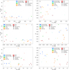 |
Fig. E.2 Distance of the cores from the closest Class I/II (top row) or Class III YSO candidate (middle row) or O/B star (bottom row) plotted against dust temperature and gas pressure ratio. The spread of the values is declining as the distance between the cores and Class I/II candidates grow but such trend cannot be seen in the cases of Class III candidates or the O/B stars. |
Appendix F Dust correlation plots
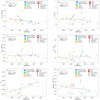 |
Fig. F.1 NH3 (1,1) and (2,2) line width, gas pressure ratio, (1,1) main hyperfine component optical depth, kinetic temperature and column density plotted against the size of the cores calculated from Herschel dust data. The filled points mark the reliable sample, the open points the candidate sample. The grey line indicates a linear fit for the two parameters for the whole sample, the black line for the reliable sample. The Pearson correlation coefficients are noted with the same colours. |
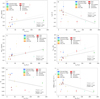 |
Fig. F.2 NH3 (1,1) and (2,2) line width, gas pressure ratio, (1,1) main hyperfine component optical depth, kinetic temperature and column density plotted against the bolometric luminosity of the cores calculated from Herschel dust data. Core #1 with its 4032 L0 has been excluded from these plots due to its extremely high Lbol compared to the rest of the sample. The filled points mark the reliable sample, the open points the candidate sample. The grey line indicates a linear fit for the two parameters for the whole sample, the black line for the reliable sample. The Pearson correlation coefficients are noted with the same colours. |
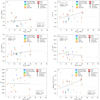 |
Fig. F.3 NH3 (1,1) and (2,2) line width, gas pressure ratio, (1,1) main hyperfine component optical depth, kinetic temperature and column density plotted against the mass of the cores calculated from Herschel dust data. The filled points mark the reliable sample, the open points the candidate sample. The grey line indicates a linear fit for the two parameters for the whole sample, the black line for the reliable sample. The Pearson correlation coefficients are noted with the same colours. |
References
- Andre, P., Ward-Thompson, D., & Barsony, M. 2000, in Protostars and Planets IV, eds. V. Mannings, A.P. Boss, & S.S. Russell, 59 [Google Scholar]
- Aspin, C. 1998, A&A, 335, 1040 [NASA ADS] [Google Scholar]
- Bastian, N., Gieles, M., Efremov, Y. N., & Lamers, H. J. G. L. M. 2005, A&A, 443, 79 [NASA ADS] [CrossRef] [EDP Sciences] [Google Scholar]
- Bertoldi, F. 1989, ApJ, 346, 735 [Google Scholar]
- Bertoldi, F., & McKee, C. F. 1992, ApJ, 395, 140 [NASA ADS] [CrossRef] [Google Scholar]
- Bouhafs, N., Rist, C., Daniel, F., et al. 2017, MNRAS, 470, 2204 [NASA ADS] [CrossRef] [Google Scholar]
- Cambrésy, L., Marton, G., Feher, O., Tóth, L. V., & Schneider, N. 2013, A&A, 557, A29 [Google Scholar]
- Cárdenas, S. B., Cichowolski, S., Suad, L. A., et al. 2022, MNRAS, 509, 3395 [Google Scholar]
- Danby, G., Flower, D. R., Valiron, P., Schilke, P., & Walmsley, C. M. 1988, MNRAS, 235, 229 [NASA ADS] [CrossRef] [Google Scholar]
- Deharveng, L., Zavagno, A., & Caplan, J. 2005, A&A, 433, 565 [NASA ADS] [CrossRef] [EDP Sciences] [Google Scholar]
- di Francesco, J., Sadavoy, S., Motte, F., et al. 2010, A&A, 518, A91 [Google Scholar]
- Elia, D., Molinari, S., Schisano, E., et al. 2017, MNRAS, 471, 100 [NASA ADS] [CrossRef] [Google Scholar]
- Elia, D., Merello, M., Molinari, S., et al. 2021, MNRAS, 504, 2742 [NASA ADS] [CrossRef] [Google Scholar]
- Elmegreen, B. G. 1998, ASP Conf. Ser., 148, 150 [Google Scholar]
- Elmegreen, B. G., & Lada, C. J. 1977, ApJ, 214, 725 [Google Scholar]
- Fehér, O., Tóth, L. V., Ward-Thompson, D., et al. 2016, A&A, 590, A75 [Google Scholar]
- Friesen, R. K., Di Francesco, J., Shirley, Y. L., & Myers, P. C. 2009, ApJ, 697, 1457 [Google Scholar]
- Friesen, R. K., Pineda, J. E., co-PIs, et al. 2017, ApJ, 843, 63 [NASA ADS] [CrossRef] [Google Scholar]
- Gritschneder, M., Naab, T., Walch, S., Burkert, A., & Heitsch, F. 2009, ApJ, 694, L26 [NASA ADS] [CrossRef] [Google Scholar]
- Harju, J., Walmsley, C. M., & Wouterloot, J. G. A. 1993, A&AS, 98, 51 [NASA ADS] [Google Scholar]
- Harju, J., Pineda, J. E., Vasyunin, A. I., et al. 2020, ApJ, 895, 101 [NASA ADS] [CrossRef] [Google Scholar]
- Hennemann, M., Motte, F., Bontemps, S., et al. 2010, A&A, 518, L84 [NASA ADS] [CrossRef] [EDP Sciences] [Google Scholar]
- Heyer, M. H., Williams, J. P., & Brunt, C. M. 2006, ApJ, 643, 956 [NASA ADS] [CrossRef] [Google Scholar]
- Ho, P. T. P., & Townes, C. H. 1983, ARA&A, 21, 239 [NASA ADS] [CrossRef] [Google Scholar]
- Juvela, M., Harju, J., Ysard, N., & Lunttila, T. 2012, A&A, 538, A133 [NASA ADS] [CrossRef] [EDP Sciences] [Google Scholar]
- Kauffmann, J., Pillai, T., & Goldsmith, P. F. 2013, ApJ, 779, 185 [NASA ADS] [CrossRef] [Google Scholar]
- Kennicutt, R. C. 2005, in IAU Symposium, 227, 3 [NASA ADS] [CrossRef] [Google Scholar]
- Keown, J., Di Francesco, J., Kirk, H., et al. 2017, ApJ, 850, 3 [NASA ADS] [CrossRef] [Google Scholar]
- Keown, J., Di Francesco, J., Rosolowsky, E., et al. 2019, ApJ, 884, 4 [Google Scholar]
- Kuhn, M. A., Hillenbrand, L. A., Sills, A., Feigelson, E. D., & Getman, K. V. 2019, ApJ, 870, 32 [CrossRef] [Google Scholar]
- Lada, C. J., Bergin, E. A., Alves, J. F., & Huard, T. L. 2003, ApJ, 586, 286 [NASA ADS] [CrossRef] [Google Scholar]
- Lefloch, B., & Lazareff, B. 1994, A&A, 289, 559 [NASA ADS] [Google Scholar]
- Li, C., Wang, H., Zhang, M., et al. 2018, ApJS, 238, 10 [NASA ADS] [CrossRef] [Google Scholar]
- Li, D., Goldsmith, P. F., & Menten, K. 2003, ApJ, 587, 262 [NASA ADS] [CrossRef] [Google Scholar]
- Liu, T., Zhang, Q., Kim, K.-T., et al. 2016, ApJS, 222, 7 [NASA ADS] [CrossRef] [Google Scholar]
- Lowe, V., Cunningham, M. R., Urquhart, J. S., et al. 2014, MNRAS, 441, 256 [NASA ADS] [CrossRef] [Google Scholar]
- Lu, X., Zhang, Q., Liu, H. B., Wang, J., & Gu, Q. 2014, ApJ, 790, 84 [NASA ADS] [CrossRef] [Google Scholar]
- Lumsden, S. L., Hoare, M. G., Urquhart, J. S., et al. 2013, ApJS, 208, 11 [Google Scholar]
- Mangum, J. G., Wootten, A., & Mundy, L. G. 1992, ApJ, 388, 467 [NASA ADS] [CrossRef] [Google Scholar]
- Marton, G., Tóth, L. V., Paladini, R., et al. 2016, MNRAS, 458, 3479 [Google Scholar]
- Mazumdar, P., Wyrowski, F., Colombo, D., et al. 2021a, A&A, 650, A164 [NASA ADS] [CrossRef] [EDP Sciences] [Google Scholar]
- Mazumdar, P., Wyrowski, F., Urquhart, J. S., et al. 2021b, A&A, 656, A101 [NASA ADS] [CrossRef] [EDP Sciences] [Google Scholar]
- Montillaud, J., Juvela, M., Vastel, C., et al. 2019, A&A, 631, A1 [NASA ADS] [CrossRef] [EDP Sciences] [Google Scholar]
- Mookerjea, B. 2022, ApJ, 926, 4 [NASA ADS] [CrossRef] [Google Scholar]
- Motte, F., Schilke, P., & Lis, D. C. 2003, ApJ, 582, 277 [NASA ADS] [CrossRef] [Google Scholar]
- Motte, F., Bontemps, S., Schilke, P., et al. 2007, A&A, 476, 1243 [NASA ADS] [CrossRef] [EDP Sciences] [Google Scholar]
- Motte, F., Zavagno, A., Bontemps, S., et al. 2010, A&A, 518, A77 [Google Scholar]
- Motte, F., Bontemps, S., & Louvet, F. 2018, ARA&A, 56, 41 [NASA ADS] [CrossRef] [Google Scholar]
- Ott, M., Witzel, A., Quirrenbach, A., et al. 1994, A&A, 284, 331 [NASA ADS] [Google Scholar]
- Ott, J., Weiss, A., Henkel, C., & Walter, F. 2005, ApJ, 629, 767 [NASA ADS] [CrossRef] [Google Scholar]
- Ott, J., Henkel, C., Braatz, J. A., & Weiß, A. 2011, ApJ, 742, 95 [NASA ADS] [CrossRef] [Google Scholar]
- Pabst, C., Higgins, R., Goicoechea, J. R., et al. 2019, Nature, 565, 618 [NASA ADS] [CrossRef] [Google Scholar]
- Phelps, R. L., & Lada, E. A. 1997, ApJ, 477, 176 [NASA ADS] [CrossRef] [Google Scholar]
- Pickett, H. M., Poynter, R. L., Cohen, E. A., et al. 1998, J. Quant. Spec. Radiat. Transf., 60, 883 [Google Scholar]
- Poulton, C. J., Robitaille, T. P., Greaves, J. S., et al. 2008, MNRAS, 384, 1249 [NASA ADS] [CrossRef] [Google Scholar]
- Ragan, S. E., Bergin, E. A., & Wilner, D. 2011, ApJ, 736, 163 [NASA ADS] [CrossRef] [Google Scholar]
- Rodgers, A. W., Campbell, C. T., & Whiteoak, J. B. 1960, MNRAS, 121, 103 [NASA ADS] [CrossRef] [Google Scholar]
- Rohlfs, K., & Wilson, T. L. 2004, Tools of radio astronomy (Berlin: Springer) [Google Scholar]
- Román-Zúñiga, C. G., & Lada, E. A. 2008, Star Formation in the Rosette Complex, ed. B. Reipurth, 4, 928 [Google Scholar]
- Román-Zúñiga, C. G., Elston, R., Ferreira, B., & Lada, E. A. 2008, ApJ, 672, 861 [CrossRef] [Google Scholar]
- Rosolowsky, E. W., Pineda, J. E., Foster, J. B., et al. 2008, ApJS, 175, 509 [Google Scholar]
- Schneider, N., Stutzki, J., Winnewisser, G., Poglitsch, A., & Madden, S. 1998, A&A, 338, 262 [NASA ADS] [Google Scholar]
- Schneider, N., Motte, F., Bontemps, S., et al. 2010, A&A, 518, A83 [Google Scholar]
- Schneider, N., Csengeri, T., Hennemann, M., et al. 2012, A&A, 540, A11 [Google Scholar]
- Schneider, N., Simon, R., Guevara, C., et al. 2020, PASP, 132, 104301 [NASA ADS] [CrossRef] [Google Scholar]
- Shipman, R. F., & Clark, F. O. 1994, ApJ, 422, 153 [NASA ADS] [CrossRef] [Google Scholar]
- Swift, J. J., Welch, W. J., & Di Francesco, J. 2005, ApJ, 620, 823 [NASA ADS] [CrossRef] [Google Scholar]
- Tafalla, M., Myers, P. C., Caselli, P., & Walmsley, C. M. 2004, A&A, 416, 191 [NASA ADS] [CrossRef] [EDP Sciences] [Google Scholar]
- Tan, J. C., Beltrán, M. T., Caselli, P., et al. 2014, in Protostars and Planets VI, eds. H. Beuther, R.S. Klessen, C.P. Dullemond, & T. Henning, 149 [Google Scholar]
- Thompson, M. A., Urquhart, J. S., Moore, T. J. T., & Morgan, L. K. 2012, MNRAS, 421, 408 [NASA ADS] [Google Scholar]
- Townes, C. H., & Schawlow, A. L. 1975, Microwave spectroscopy (New York, USA: Dover Publications) [Google Scholar]
- Ungerechts, H., Walmsley, C. M., & Winnewisser, G. 1986, A&A, 157, 207 [Google Scholar]
- Urquhart, J. S., Figura, C. C., Moore, T. J. T., et al. 2014, MNRAS, 437, 1791 [NASA ADS] [CrossRef] [Google Scholar]
- Urquhart, J. S., Figura, C. C., Moore, T. J. T., et al. 2015, MNRAS, 452, 4029 [NASA ADS] [CrossRef] [Google Scholar]
- Veltchev, T. V., Ossenkopf-Okada, V., Stanchev, O., et al. 2018, MNRAS, 475, 2215 [Google Scholar]
- Walmsley, C. M., & Ungerechts, H. 1983, A&A, 122, 164 [Google Scholar]
- Wang, J., Townsley, L. K., Feigelson, E. D., et al. 2008, ApJ, 675, 464 [NASA ADS] [CrossRef] [Google Scholar]
- Wareing, C. J., Pittard, J. M., Wright, N. J., & Falle, S. A. E. G. 2018, MNRAS, 475, 3598 [NASA ADS] [CrossRef] [Google Scholar]
- Weidner, C., Pflamm-Altenburg, J., & Kroupa, P. 2011, ASP Conf. Ser., 440, 19 [NASA ADS] [Google Scholar]
- Wienen, M., Wyrowski, F., Schuller, F., et al. 2012, A&A, 544, A146 [NASA ADS] [CrossRef] [EDP Sciences] [Google Scholar]
- Wienen, M., Wyrowski, F., Menten, K. M., et al. 2018, A&A, 609, A125 [NASA ADS] [CrossRef] [EDP Sciences] [Google Scholar]
- Williams, J. P., Blitz, L., & Stark, A. A. 1995, ApJ, 451, 252 [NASA ADS] [CrossRef] [Google Scholar]
- Yi, H.-W., Lee, J.-E., Liu, T., et al. 2018, ApJS, 236, 51 [NASA ADS] [CrossRef] [Google Scholar]
- Yi, H.-W., Lee, J.-E., Kim, K.-T., et al. 2021, ApJS, 254, 14 [NASA ADS] [CrossRef] [Google Scholar]
- Zhang, Q., Qiu, K., Girart, J. M., et al. 2014, ApJ, 792, 116 [Google Scholar]
- Zinnecker, H., & Yorke, H. W. 2007, ARA&A, 45, 481 [Google Scholar]
All Tables
Parameters of the cores from Motte et al. (2010) and Hennemann et al. (2010) selected for our sample.
Parameters calculated from the NH3 (1,1) and (2,2) with the average, minimum, maximum, and median values of each parameter and their respective standard deviations obtained from the MC calculation.
All Figures
|
Fig. 1 Overview of the Rosette Nebula on a Berschel SPIRE 250 µm surface brightness map. The cores observed at Effelsberg are shown with different colours, which indicate their evolutionary stages derived from Berschel data by Motte et al. (2010): (green) warm-starless, (blue) prestellar, (red) protostellar core. The yellow dots represent the stars of the cluster NGC 2244. The white and purple stars mark the O and B stars of the cluster, respectively. The areas indicated by black rectangles and the YSO clusters indicated by yellow circles are presented in Sect. 1. The inserts give a closer look at areas PL03, Shell, Center, and AFGL 961 in order to clearly distinguish our sources. |
| In the text | |
|
Fig. 2 Example of ammonia inversion transition spectra for core #71. Top: NH3 (1,1) spectrum shifted on the y-axis by 1 K. The orange line shows the CLASS hyperfine best fit obtained. Bottom: NH3 (2,2) spectrum. The blue line shows the Gaussian best fit. The best-fit centroid velocity, peak Tmb, FWHM, and S/N are included for both transitions. |
| In the text | |
|
Fig. 3 Distributions of the obtained parameters according to the evolutionary stages of the sources covering both the reliable and the candidate sample. The colours represent warm-starless, protostellar, and prestellar cores, and the black outline represents the whole sample, as indicated in the legend. The histograms are (a) NH3 (1,1) line width, (b) NH3 (2,2) line width, (c) NH3 (1,1) main hyperfine component optical depth – all of which are from CLASS fitting (see Sect. 2.2) –, (d) thermal line width calculated from Eq. (6), (e) kinetic temperature calculated from Eq. (2), and (f) NH3 column density calculated from Eq. (13). |
| In the text | |
|
Fig. 4 NH3 (1,1) and (2,2) line widths with their errors. The red line marks equal widths. The warm-starless, prestellar, and protostellar cores are indicated with squares, circles, and stars, respectively. The colours represent the areas where the cores are from (see Fig. 1). The filled points mark the reliable sample, the open points the candidate sample. The point that has a (2,2) FWHM of 5.15 km s−1 has been excluded from further analysis based on its broad line width. |
| In the text | |
|
Fig. 5 Distribution of the (a) gas pressure ratios and (b) virial parameters. The low gas pressure ratio of the warm-starless core #8 may suggest a more turbulent line width for these types of cores. However, this core is not depicted in the bottom panel because of its significantly higher α of 12.32. |
| In the text | |
|
Fig. 6 (a) NH3 (1,1) line width, (b) kinetic temperature, (c) gas pressure ratio, and (d) column density plotted against the projected distance of the cores from NGC 2244. The filled points mark the reliable sample, the open points the candidate sample. The black and the grey lines indicate a running median of the values using non-uniform binning for the reliable and for the whole sample, respectively. The distances are shown in degrees with 1° corresponding to 28 pc at a distance of 1.6 kpc. |
| In the text | |
|
Fig. 7 Integrated NH3 intensity from Keown et al. (2019) in K km s−1. The red contours show the Herschel dust emission at 250 µm. In the central map, the grey area indicates the zone not covered by Keown et al. (2019) observations, and the contour is at level 400 MJy sr−1. In the close up views of the region, the contours are at levels of 400, 500, and 600 MJy sr−1 for the Monoceros Ridge and the Extended Ridge; at 400, 500, 1000, and 1500 MJy sr−1 for PL03; at 400, 500, 1000, and 2000 MJy sr−1 for the Shell; at 400, 500, 1000, 2000, and 4000 MJy sr−1 for AFGL 961; and at 600, 800, 1000, 1200, and 1400 MJy sr−1 for the Center. The open squares show the Effelsberg targets with the same colour code as in Fig. 1. |
| In the text | |
|
Fig. 8 Spatial shift between the NH3 and dust maxima for targets where both KEYSTONE and Herschel data are available. For the missing sources, no maxima are visible for at least one dataset. The colours show the region hosting the source as mentioned in the legend. The shift of Δα = −18″, Δδ = 13″ corresponds to the isolated source east of the Center region. The circles have 10″ and 20″ radii, corresponding to 25% and 50% of the Effelsberg beam size, and to 31% and 62% of the GBT beam size. |
| In the text | |
|
Fig. 9 NH3 column density and kinetic temperature. The symbols and colours are as in Fig. 4. The grey line indicates a linear fit for the whole sample, the black line for the reliable sample. The Pearson correlation coefficients are noted with the same colours. Bottom: The red square indicates three outlier sources, which have been excluded from the correlation measurements in this panel. |
| In the text | |
|
Fig. 10 NH3 (1,1) and (2,2) line width, gas pressure ratio, (1,1) main hyperfine component optical depth, kinetic temperature, and column density plotted against dust temperature. The filled points mark the reliable sample, the open points the candidate sample. The grey line indicates a linear fit for the two parameters for the whole sample, the black line for the reliable sample. The Pearson correlation coefficients are noted with the same colours. The rest of the correlation plots for ammonia and dust parameters are included in Appendices F.1, F.2, and F.3. |
| In the text | |
|
Fig. 11 Comparison of the parameters of our sample of cores with those of different star-forming regions. (a) Kinetic temperatures and NH3 column densities, (b) kinetic temperatures and gas pressure ratios, and (c) NH3 column densities and gas pressure ratios of our sample of cores from the Rosette Molecular Cloud along with the samples from Perseus of Rosolowsky et al. (2008), from Ophiuchus of Friesen et al. (2009), from the ATLASGAL survey of Wienen et al. (2012), and from G333 of Lowe et al. (2014). The samples of Perseus and Ophiuchus show the widest range of gas pressure ratios. The red dashed line marks Rp = 1. In (c), the red and black points of Rosette overlap as the figure does not depict kinetic temperatures. The column densities of Rosolowsky et al. (2008) have lower values, ~51−53% of what the other equations used by the other samples give as a result. |
| In the text | |
|
Fig. A.1 Ammonia spectra for cores #1 to #5 and #7, as indicated in the top-right corner of each frame. In each panel, the top spectrum is the NH3 (1,1) spectrum shifted by 1 K. The orange line shows the CLASS hyperfine best fit obtained. The bottom spectrum is NH3 (2,2) spectrum. The blue line shows the Gaussian best fit. The best-fit centroid velocity, peak Tmb, FWHM, and S/N are included for both transitions. The grey parts of the spectra were outside the analysed velocity range, which were defined around the vIsr(1,1) and vIsr(2,2) values. |
| In the text | |
|
Fig. A.1 continued for cores #8 to #13 and #15 to #17. |
| In the text | |
|
Fig. A.1 continued for cores #18 to #20, #22, #24, #28, #31, #36, and #39. |
| In the text | |
|
Fig. A.1 continued for cores #41, #43, #45, #46, #49, #50, #52, #71, and #76. |
| In the text | |
|
Fig. C.1 Results of the MC simulations for core #1. Frames (a), (b), and (c) show parameters obtained for the NH3 (1,1) line, (c) and (d) for the (2,2) line. Frame (e) shows the distribution obtained for (1,1) temperature, (f) for (2,2), (g) for rotational temperature, and (h) for NH3 column density. Black crosses show the values obtained from the CLASS fitting. The red dashed lines indicate the 16, 50, and 84 percentiles, the thin black dashed lines show the standard deviation, and the thick black dashed line shows the values obtained with the best-fit parameter. |
| In the text | |
|
Fig. D.1 Correlation plots between different parameters calculated from the ammonia data. |
| In the text | |
|
Fig. E.1 Distance of the cores from the closest Class I/II (top row) or Class III YSO candidate (middle row) or O/B star (bottom row) plotted against kinetic temperature and column density. The spread of the values is declining as the distance between the cores and Class I/II candidates grow but such trend cannot be seen in the cases of Class III candidates or the O/B stars. |
| In the text | |
|
Fig. E.2 Distance of the cores from the closest Class I/II (top row) or Class III YSO candidate (middle row) or O/B star (bottom row) plotted against dust temperature and gas pressure ratio. The spread of the values is declining as the distance between the cores and Class I/II candidates grow but such trend cannot be seen in the cases of Class III candidates or the O/B stars. |
| In the text | |
|
Fig. F.1 NH3 (1,1) and (2,2) line width, gas pressure ratio, (1,1) main hyperfine component optical depth, kinetic temperature and column density plotted against the size of the cores calculated from Herschel dust data. The filled points mark the reliable sample, the open points the candidate sample. The grey line indicates a linear fit for the two parameters for the whole sample, the black line for the reliable sample. The Pearson correlation coefficients are noted with the same colours. |
| In the text | |
|
Fig. F.2 NH3 (1,1) and (2,2) line width, gas pressure ratio, (1,1) main hyperfine component optical depth, kinetic temperature and column density plotted against the bolometric luminosity of the cores calculated from Herschel dust data. Core #1 with its 4032 L0 has been excluded from these plots due to its extremely high Lbol compared to the rest of the sample. The filled points mark the reliable sample, the open points the candidate sample. The grey line indicates a linear fit for the two parameters for the whole sample, the black line for the reliable sample. The Pearson correlation coefficients are noted with the same colours. |
| In the text | |
|
Fig. F.3 NH3 (1,1) and (2,2) line width, gas pressure ratio, (1,1) main hyperfine component optical depth, kinetic temperature and column density plotted against the mass of the cores calculated from Herschel dust data. The filled points mark the reliable sample, the open points the candidate sample. The grey line indicates a linear fit for the two parameters for the whole sample, the black line for the reliable sample. The Pearson correlation coefficients are noted with the same colours. |
| In the text | |
Current usage metrics show cumulative count of Article Views (full-text article views including HTML views, PDF and ePub downloads, according to the available data) and Abstracts Views on Vision4Press platform.
Data correspond to usage on the plateform after 2015. The current usage metrics is available 48-96 hours after online publication and is updated daily on week days.
Initial download of the metrics may take a while.