| Issue |
A&A
Volume 684, April 2024
|
|
|---|---|---|
| Article Number | A142 | |
| Number of page(s) | 37 | |
| Section | Interstellar and circumstellar matter | |
| DOI | https://doi.org/10.1051/0004-6361/202345963 | |
| Published online | 18 April 2024 | |
Surveys of clumps, cores, and condensations in Cygnus X
Temperature and nonthermal velocity dispersion revealed by VLA NH3 observations★
1
School of Astronomy and Space Science, Nanjing University,
163 Xianlin Avenue,
Nanjing
210023,
PR China
e-mail: This email address is being protected from spambots. You need JavaScript enabled to view it.
2
Max-Planck-Institut für Radioastronomie,
Auf dem Hügel 69,
53121
Bonn,
Germany
3
Key Laboratory of Modern Astronomy and Astrophysics (Nanjing University), Ministry of Education,
Nanjing
210023,
PR China
4
Center for Astrophysics | Harvard & Smithsonian,
160 Concord Avenue,
Cambridge,
MA
02138,
USA
5
National Astronomical Observatory of Japan,
2-21-1 Osawa, Mitaka,
Tokyo
181-8588,
Japan
6
Shanghai Astronomical Observatory, Chinese Academy of Sciences,
80 Nandan Road,
Shanghai
200030,
PR China
Received:
20
January
2023
Accepted:
15
February
2024
Abstract
Context. The physical properties, evolution, and fragmentation of massive dense cores (MDCs, ~0.1 pc) are fundamental pieces in our understanding of high-mass star formation.
Aims. We aim to characterize the temperature, velocity dispersion, and fragmentation of the MDCs in the Cygnus X giant molecular cloud and to investigate the stability and dynamics of these cores.
Methods. We present the Karl G. Jansky Very Large Array (VLA) observations of the NH3 (J, K) = (1,1) and (2,2) inversion lines towards 35 MDCs in Cygnus X, from which we calculated the temperature and velocity dispersion. We extracted 202 fragments (~0.02 pc) from the NH3 (1,1) moment-0 maps with the GAUSSCLUMPS algorithm. We analyzed the stability of the MDCs and their NH3 fragments through evaluating the corresponding kinetic, gravitational potential, and magnetic energies and the virial parameters.
Results. The MDCs in Cygnus X have a typical mean kinetic temperature TK of ~20 K. Our virial analysis shows that many MDCs are in subvirialized states, indicating that the kinetic energy is insufficient to support these MDCs against their gravity. The calculated nonthermal velocity dispersions of most MDCs are at transonic to mildly supersonic levels, and the bulk motions make only a minor contribution to the velocity dispersion. Regarding the NH3 fragments, with TK ~19 K, their nonthermal velocity dispersions are mostly trans-sonic to subsonic. Unless there is a strong magnetic field, most NH3 fragments are probably not in virialized states. We also find that most of the NH3 fragments are dynamically quiescent, while only a few are active due to star formation activity.
Key words: stars: formation / stars: massive / ISM: kinematics and dynamics / ISM: molecules
The reduced datacubes and the table of the physical parameters of NH3 fragments are available at the CDS ftp to cdsarc.cds.unistra.fr (130.79.128.5) or via https://cdsarc.cds.unistra.fr/viz-bin/cat/J/A+A/684/A142
© The Authors 2024
 Open Access article, published by EDP Sciences, under the terms of the Creative Commons Attribution License (https://creativecommons.org/licenses/by/4.0), which permits unrestricted use, distribution, and reproduction in any medium, provided the original work is properly cited.
This article is published in open access under the Subscribe to Open model. This email address is being protected from spambots. You need JavaScript enabled to view it. to support open access publication.
1 Introduction
High-mass stars (>8 M⊙) play a vital role in shaping their host galaxies via their intense feedback effects in the form of powerful outflows, strong stellar winds, and violent UV radiation (Motte et al. 2018). However, the formation of high-mass stars is still an open question. Unlike the star formation model built in low-mass stars (Shu et al. 1993), accretion onto high-mass protostars is difficult to model because of the radiation pressure problem (Wolfire & Cassinelli 1987) and the violent wind (Krumholz 2015). In observations, it is difficult to catch the high-mass stellar embryos as their birthplaces are usually far away and deeply embedded (Zinnecker & Yorke 2007). The small populations and short timescales of critical evolutionary phases mean that the sample of high-mass stellar embryos is even more insufficient (Zinnecker & Yorke 2007).
Several candidate theories of high-mass star formation have been proposed, such as competitive accretion in protostellar clusters (Bonnell et al. 1997, 2001), mergers of protostars (Bonnell et al. 1998), turbulent core accretion (McKee & Tan 2003), and inertial inflow (Padoan et al. 2020). To verify these theories, it is necessary to observationally investigate the initial conditions of high-mass star formation. Observations with a range of tracers in a variety of wavelengths and resolutions have been carried out towards massive dense cores (MDCs), the possible birth places of high-mass stars (e.g., Beuther et al. 2002; Motte et al. 2007; Lu et al. 2014; Rathborne et al. 2016; Cao et al. 2019; Zhang et al. 2019). By characterizing the physical conditions of high-mass star formation with observations, we can test and provide practical constraints to the corresponding theories.
The CENSUS project (Surveys of Clumps, CorEs, and CoNdenSations in CygnUS X, PI: Keping Qiu) is dedicated to a systematic study of the 0.01–10 pc hierarchical molecular structures and the high-mass star formation process in the molecular complex Cygnus X. In order to investigate the temperature structures and dynamic conditions of MDCs in our project, we make use of the NH3 (1,1) and (2,2) inversion emission lines, which trace gas with critical density of ~104 cm−3 and excitation temperature of ~10–30 K (Ho & Townes 1983; Mangum & Shirley 2015). These lines are widely used for studying the initial conditions of star formation. Previous NH3 surveys find a mean temperature of ≲ 15 K in less-evolved structures and ~20 K in protostellar cores with significant star-forming activity (e.g., Pillai et al. 2006; Wu et al. 2006; Chira et al. 2013; Kerr et al. 2019). The velocity dispersion of these lines is found to be dominated by nonthermal components in most cases (e.g., Lu et al. 2014; Billington et al. 2019). Furthermore, analyses of the dynamical stability of star-forming structures at various scales and evolutionary stages can be done with these lines via the virial analysis (e.g., Jijina et al. 1999; Zhang et al. 2020). Therefore, a high-resolution unbiased NH3 survey towards the MDCs in the Cygnus X cloud complex offers a remarkable observational sample that can be used to unravel the initial conditions of high-mass star formation.
The Cygnus X cloud, located at 1.4 kpc from the Sun (Rygl et al. 2012), is one of the richest and most active molecular and HII complexes in the Galaxy. It is massive (~4 × 10⁶ M⊙) and large (extends over ~100 pc in diameter; Leung & Thaddeus 1992), and consists of substantial HII regions (Wendker et al. 1991) and OB associations (Uyanıker et al. 2001). All these features make Cygnus X an ideal object for studying high-mass star formation. Several surveys and numerous case studies towards Cygnus X have been carried out over recent decades (e.g., Motte et al. 2007; Gottschalk et al. 2012; Takekoshi et al. 2019). The CENSUS project has published several works on Cygnus X: Cao et al. (2019) generated a complete sample of MDCs in Cygnus X and performed an analysis of their far-infrared emission; Wang et al. (2022) provide radio continuum views of the MDCs; Pan et al. (2024) provide a survey of the possible circumstellar disks in Cygnux X; Yang et al. (2024) analyzed the high-velocity outflow using Submillimeter Array (SMA) observations of SiO (5–4). In the CENSUS project, we adopt the terminology that clumps, cores, and condensations correspond to cloud structures of a physical full width at half maximum (FWHM) size of ~1, ~0.1, and ~0.01 pc, respectively, which is also widely used in other studies (e.g., Pokhrel et al. 2018; Zhang et al. 2019).
As a part of CENSUS, we report an unbiased NH3 survey towards 37 fields in Cygnus X observed with the Karl G. Jansky Very Large Array (VLA) with a spatial resolution of ~0.02 pc. This paper is organized as follows. Section 2 outlines details of the sample and observational setups. In Sect. 3, we describe the methods we used to analyze the NH3 data. The derived physical parameters and their distributions and correlations are presented in Sect. 4. The NH3 morphology, a virial analysis, the dynamical states of MDCs, and a comparison between dust and gas temperatures are discussed in Sect. 5. Finally, the study is summarized in Sect. 6, where we outline our conclusions.
2 Sample and observations
2.1 Sample selection
The interferometer observations of the CENSUS project (PI: Keping Qiu, also see Cao et al. 2019) were designed to target most MDCs in Cygnus X (Wang et al. 2022). We first selected 42 sources with estimated masses of greater than 30 M⊙ from Motte et al. (2007), though one source (S26) was later found to be outside of Cygnus X (Rygl et al. 2012) and another (N58) should have a much lower mass (see Table 1 for more details). In this work, we exclude 10 sources in the DR 21 region, which were observed by the VLA in a mosaic setup (Project ID: 14A-241; PI: Qizhou Zhang) and will be presented in a separate work. The other 32 sources, as well as an additional source (NW12, see Table 1 for more details), were observed with the VLA in 29 fields. In the present work, we also include VLA observations of another eight fields covering bright JCMT SCUBA-2 sources (Cao et al. 2019) located in the OB2 association region1. Here, VLA observations of a total of 37 fields are therefore presented (Table 1). As part of the CENSUS project, Cao et al. (2021) constructed a column density map of the entire Cygnus X complex based on SED fitting of multiband Herschel observations and extracted more than 8000 cores with the getsources algorithm. In the following analysis, we adopt the parameters of dense cores from Cao et al. (2021).
2.2 Very Large Array
The NH3 data were obtained from the NRAO2 VLA program 17A-107 (PI: Keping Qiu), which observed with 27 antennas in the D-array configuration. The program 17A-107 is an unbiased and high-resolution survey dedicated to observing the NH3 (J,K)=(1,1), (2,2), (3,3), (4,4), and (5,5) rotation-inversion transitions, CCS (1,2-2,1) and CCS (6,5-5,5) emissions, and H2O maser lines for MDCs in Cygnus X. The baselines of the array range from 0.035 km to 1.03 km, corresponding to the largest recoverable angular scale of ~66″ (0.45 pc for Cygnus X) and an angular resolution of ~3″.1 (0.02 pc for Cygnus X), respectively. The correlator setup provides eight independent spectral windows with a spectral channel spacing of 7.8 kHz and a bandwidth of 8 MHz, corresponding to a velocity resolution of 0.1 km s−1 and a velocity coverage of 100 km s−1 for the NH3 (1,1) and (2,2) lines.
The VLA data were calibrated using the Common Astronomy Software Applications (CASA) package (McMullin et al. 2007). The flux calibrator and bandpass calibrator were both set as the quasar 1331+305 (3C286). Gain calibration was performed with observations of J2007+4029. The calibrated data were imaged using the CASA task clean, gridded with a pixel size of 1″. The rms of these fields is ≲ 0.013 Jy beam−1 in a 0.1 km s−1 channel width. The coordinates of the field centers and noise levels are also listed in Table 1. The NH3 (1,1) and (2,2) emission lines are the main interests of this paper. The rest frequencies of the (1,1) and (2,2) emission lines are 23.6945 and 23.72263 GHz, while upper energy levels are 23.4 and 64.9 K, respectively. Observations of the other spectral lines in 17A-107 are beyond the scope of this paper, and are listed in Appendix A.
2.3 MIR archive data from the Spitzer Space Telescope
We use the Spitɀer IRAC 3.6, 4.5, and 8.0 µm data from the Spitɀer Legacy Survey of the Cygnus X Complex3 (Kraemer et al. 2010) in this paper, which are downloaded from the NASA/IPAC Infrared Science Archive4. All these data cover the entire Cygnus X region, with a pixel size of 2″ and 1σ rms noise levels of 25.1, 27.1, and 47.9 MJy sr−1, respectively.
3 Methods
We checked detections in all data cubes before fitting the NH3 lines. In order to determine whether there is detection in a spectrum, the NH3 (1,1) data cubes are smoothed to a velocity resolution of 0.7 km s−1, or seven spectral channels in our observations, to improve signal-to-noise ratios (S/Ns). The criterion of significant detection within a beam is set as S/N ≥ 5 in the smoothed NH3 (1,1) data. The corresponding original spectra were fitted in the following processes if their smoothed spectra exceeded the threshold. The detections and noise levels in all the fields are reported in Table 2. The detections in fields are marked as marginal if the emissions are only detected in one or two beams. We adopt the distance of 1.4 kpc (Rygl et al. 2012) for all the fields except for Field 21 (also known as AFGL2591), of which the distance is 3.3 kpc (Rygl et al. 2012).
3.1 Ammonia line fitting
Following the theoretical framework in Mangum & Shirley (2015), we built spectral models of the NH3 (1,1) and (2,2) emission with the centroid velocity, line width, excitation temperature, NH3 column density in the upper transition state, and beam-filling factor as free parameters and with the following assumptions: (1) the same beam-filling factor and excitation temperature for all hyperfine transitions; (2) local thermodynamic equilibrium (LTE). The NH3 (1,1) and (2,2) data cubes were fitted simultaneously using the model to derive the aforementioned physical parameters.
We can get the relationship between the brightness temperature and excitation temperature as
 (1)
(1)
where f is the beam-filling factor and Tbg is the background temperature. We take the temperature of cosmic microwave background (CMB) as Tbg, which is 2.73K. The optical depth τν can be written as
 (2)
(2)
where Nu is the column density of molecules in the upper transition state. Here, we assume a Gaussian profile,
 (3)
(3)
where v0 is the central frequency of the emission. The Einstein coefficient Aul is
 (4)
(4)
where µlu and Rs are the permanent dipole moment of NH3 and the relative strengths of the hyperfine structures, respectively. In our model, Rs is set as 1/2, 5/36, and 1/9 for the main, inner satellite, and outer satellite components of NH3 (1,1) emission, respectively. As for the main and inner satellite components of NH3 (2,2) emission, Rs is set as 0.796 and 0.052, respectively. We can derive the total NH3 column density Ntot from the relationship between Nu and Ntot (Boltzmann distribution),
 (5)
(5)
where the rotation partition function  , and gu is the total degeneracy for the upper energy level, which can be found in Mangum & Shirley (2015).
Using these formulas, we built a blended spectral model rather than the all-hyperfine model after comparing their fitted results. This model consists of five Gaussian components for NH3 (1,1) emission and three Gaussian components for NH3 (2,2) emission. We do not include the two outer satellite components in our model as most NH3 (2,2) lines do not show remarkable satellite components in our data. The excitation temperature and the column density are derived only when the S/Ns of the (2,2) moment-0 maps are greater than 2 in order to avoid large uncertainties.
We then fitted the NH3 (1,1) and (2,2) simultaneously with five Gaussian components for (1,1) emission and three Gaussian components for (2,2) emission. An example result is shown in Fig. 1.
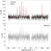 |
Fig. 1 Example five-component-fitting results on NH3 (1,1) and (2,2) emission (pixel coordinate (142,131) in Field 3). Upper panel: original spectrum and the fitted result are colored in black and red, respectively. Lower panel: residual spectrum of this fitting result. |
3.2 Temperature threshold and kinetic temperature
Regarding the NH3 inversion emission lines, the excitation temperature refers to the rotation temperature of NH3, Trot. We set the upper limit and lower limit of Trot in the fitting processes to 50 K and 8 K, respectively. The lower limit refers to the typical temperature of interstellar molecular clouds without starforming activity, that is, ~ 10K, and the upper bound corresponds to the fact that the NH3 (1,1) and (2,2) lines cannot be a good temperature probe when the Trot of the gas exceeds ~30 K.
To obtain the kinetic temperature, TK, from Trot, we employ the empirical approximation provided by Ott et al. (2011),
 (6)
(6)
The temperature mentioned hereafter refers to the kinetic temperature.
Tafalla et al. (2004) and Swift et al. (2005) also derived Trot–TK relations. Comparing these results, we find that the empirical approximation from Ott et al. (2011) applies for a wider range of Trot (Trot < 500 K), while the ranges are 5 K < Trot < 20 K and TK ≪ 41 K for the relations in Tafalla et al. (2004) and Swift et al. (2005), respectively. In our results, a remarkable number of detections are hotter than 20 K, which is why we choose the relation from Ott et al. (2011).
Observational fields and related MDCs.
3.3 Intrinsic line width and velocity dispersion
The line width derived from our fitting is blended by several hyperfine lines, because we do not conduct the full-hyperfine fitting. To derive the intrinsic line width that truly reflects the gas motion, we firstly subtract the channel width (0.1 km s−1) from the FWHM line widths derived from the line fitting quadratically. We then apply the following empirical relation of Barranco & Goodman (1998) to eliminate the effect of hyperfine-line blending:
 (7)
(7)
where Cn(τ0) is given as
 (8)
(8)
Here, τ0 is the total optical depth of NH3 (1,1) emission. We take the optical depth of the NH3 (1,1) main line, τ11,m, as the approximation of τ0. The conversion coefficient, Knm, is listed in Table 3. As a polyfit result, this relation has its limitations for large FWHM line widths, which will make ∆υint larger than ∆υblended. In this case, we use ∆υblended as an approximation of ∆υint; that is, ∆υint ≈ ∆υblended. Furthermore, we also tested the full-hyperfine fitting in Fields 3 and 5 and compared the fitted line width with that derived from our fitting results. In Field 3, the mean and median differences between the line widths from these two fitting methods are 0.034 and 0.027 km s−1 (5.4% and 6.7% for relative deviations, respectively). Regarding Field 5, these values are 0.062 (2.4%) and 0.008 (1.5%) km s−1, respectively. The empirical relation is therefore reliable and the differences are totally negligible.
The intrinsic line width can be further decomposed into  , where
  is the thermal velocity dispersion of NH3 and συ,NT is the nonthermal component. We can calculate the thermal velocity dispersion via
  . Thus, we can derive the nonthermal velocity dispersion συ,NT. Taking the molecular weight per mean free particle of typical interstellar molecular gas as 2.33 mH (Kauffmann et al. 2008), we can calculate the thermal velocity dispersion of the whole molecular gas,
  . We then derive the total velocity dispersion for the whole molecular gas from
 (9)
(9)
We refer to συ when we discuss velocity dispersion in the following context.
Detections in each field.
Values of Knm.
3.4 Uncertainties of the results
The uncertainties of the derived physical parameters could originate from both the observational process and the data reduction, including the missing flux, the calibration errors, the systematic errors of the calculating algorithms we use, and so on. The uncertainty of kinetic temperatures comes from two processes: the calculation of Trot and the transformation from Trot to TK. Here, Trot is mainly determined by the ratio of the main components of the NH3 (1,1) and (2,2) inversion lines. In this process, the uncertainty of Trot is ~10.3/S/N K, where S/N is the signal-to-noise ratio of the NH3 (2,2) inversion line (Li et al. 2003). The S/Ns of our results range from ~2 to ≳ 15, corresponding to the rms errors from ~5.2 to ≲0.69 K. For the transformation process, we expect an uncertainty of ~4 K according to Ott et al. (2011).
Regarding the velocity dispersion, there are three physical parameters involved in its calculation: the blended line width, the optical depth, and the kinetic temperature. The optical depth has little effect on the calculation of intrinsic line width (Barranco & Goodman 1998). According to Lu et al. (2014), the uncertainty of the blended line width can be written as
 (10)
(10)
where F is the flux intensity. δF/F is estimated to be ~30% in our data, indicating an uncertainty on the blended line width of ~15%. The empirical relation between ∆υint and ∆υblended would increase this uncertainty to about 30%. Coupled with the uncertainty of kinetic temperatures, the uncertainty of the velocity dispersion could be ≳30%.
4 Results
4.1 Moment-0 paps and fragment extraction
In order to show the distributions of the spectral lines, we produce the moment-0 maps of all fields by integrating their intensities in the velocity ranges of the NH3 (1,1) main components. The NH3 (1,1) and (2,2) moment-0 maps of Field 3 are shown as an example in Fig. 2. The NH3 (1,1) and (2,2) moment-0 maps are plotted from 3σ and 2σ levels, respectively. Moment-0 maps of other fields and the other emission lines are presented in Appendix A.
As mentioned in Sect. 1, the NH3 (1,1) moment-0 maps could roughly illustrate the distribution of cold dense gas in our MDCs. We extracted 202 fragments from the NH3 (1,1) moment-0 maps using the Starlink GAUSSCLUMPS algorithm (Berry et al. 2007; Currie et al. 2014). The field 21 was excluded from the extraction as it is not at the distance of Cygnus X. The results of the identified NH3 fragments in Field 3 are also plotted in Fig. 2 with blue ellipses. In addition, the sizes of NH3 fragments are defined as the deconvolved radius, following
 (11)
(11)
where a and b are the semi-major and semi-minor axes of NH3 fragments.
We also show the positions of the condensations identified in the SMA 1.3 mm continuum data from Cao et al. (2021). There are 148 condensations overlapping with the fields in this paper. The majority of them (103 out of 148) are distributed in the identified NH3 fragments, indicating that the NH3 fragments can probe the density structures well in most cases. As shown in Fig. 3, the (1,1) main components of most NH3 fragments have moderate optical depths, and the mean and median values are 2.2 and 1.9. Under such a moderate optical depth, the NH3 (1,1) lines might show different morphologies from the density profiles of the dust continuum emission, which could account for the condensations uncorrelated to the NH3 fragments. In conclusion, the majority of the NH3 fragments can be considered as density structures.
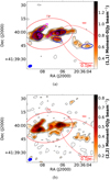 |
Fig. 2 (a) Moment-0 map of the NH3 (1,1) line for Field 3. The contour is plotted from 3σ level and in steps of 2σ. The red ellipses show the MDCs identified from the H2 column density map (resolution ~20″) by Cao et al. (2021), and the blue ellipses illustrate the fragments extracted using the GAUSSCLUMPS algorithm. The magenta boxes show the condensations identified from the SMA 1.3 mm continuum, (b) Moment-0 map of the NH3 (2,2) line for Field 3. The contour is plotted from 2σ level and in steps of 2σ. |
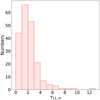 |
Fig. 3 Histogram of the average optical depth of the main component of the NH3 (1,1) line for identified NH3 fragments. |
4.2 Maps of the derived physical parameters
The line-fitting process of the NH3 (1,1) and (2,2) emission lines provides the spatial distributions of the kinetic temperature, centroid velocity, velocity dispersion, optical depth of the NH3 (1,1) main component, NH3 column density, and the beam-filling factor in all the fields, which allow us to investigate the temperature and dynamic conditions of the MDCs in Cygnus X and their fragments. We present maps of these derived parameters in Appendix B, and the maps of Field 3 in Fig. 4 as an example. Ranges of the derived physical parameters are listed by each field in Table 4. Using these maps, we obtain the average kinetic temperature, NH3 column density, velocity dispersion, and its nonthermal component for all the NH3 fragments. The contribution from the velocity gradients within the NH3 fragments, which is usually considered as the bulk motion, is taken into account when calculating the velocity dispersion, συ, and its nonthermal component, συ,NT. We also fit the velocity gradients (following the method in e.g., Goodman et al. 1993; Wu et al. 2018) and deduct them from the nonthermal velocity dispersions, which are provided as συ,ng. The detailed calculation can be found in Appendix E. A brief statistic analysis of these physical parameters is reported in Table 5 and the histograms of their distributions are shown in Fig. 5. The detailed physical parameters of the NH3 fragments are available in our online materials at the CDS.
Statistically, the NH3 fragments have a mean deconvolved radius of 0.02 pc thanks to the high spatial resolution of our observations. Recently, Zhang et al. (2019) obtained the same value for the typical radius of condensations from their PdBI 1.3 mm continuum observations. In the other two papers of CENSUS (Pan et al. 2024; Yang et al. 2024), the properties of condensations in the Cygnus X regions are explored in more detail using submillimeter continuum and spectral observations from SMA.
The temperatures of NH3 fragments range from ~11.0 K to 34.1 K, with mean and median values of 18.6 K and 17.5 K, respectively. The mean temperature of the condensations in Zhang et al. (2019), which are selected from several massive proto-cluster clumps, is 28.3 K, which is higher than the value found in the present study. Lu et al. (2014) derived a mean temperature of ~18.3 K for NH3 dense cores (with a typical size of ~0.08 pc) in 62 high-mass star-forming regions, which is consistent with our results. Temperature is one of the commonly used indicators of the evolutionary stage of molecular structures. For example, Sánchez-Monge et al. (2013) calculated the mean temperatures of the quiescent starless cores and the protostellar cores (with typical sizes of ~0.05 pc) as 18.8 K and 28.8 K, respectively. To verify this relation in our data, we matched the NH3 fragments with the condensations from Cao et al. (2021) and the IR sources from the Cygnus X Archive catalog (the Spitzer Cygnus X Legacy Survey, Kraemer et al. 2010). The temperature distribution of the NH3 fragments coincident with the continuum condensations (70 out of 202) is shown in Fig. 6, indicating that these fragments are more likely to be density structures. These condensation-related fragments are divided into two groups: those associated and not associated with the IR sources (44 and 26 in number). The mean temperature of the former group is 20.4±4.5 K, slightly higher than that of the latter group of 19.1 ±4.4 K. Also, their median temperature values are 19.4 K and 17.3 K. In general, those with IR sources are considered to be more evolved than those without IR sources. We performed a two-sample Kolmogorov-Smirnov test on the temperature distribution of these two groups and the p-value is calculated as 0.18. The p-value is higher than the threshold 0.05, indicating the two groups are not distinguishable. As shown in Fig. 6, there are also considerable overlaps in temperatures between the two groups, suggesting that there is no significant difference in internal heating for the sources in the two groups. Instead, we find that the morphology of the NH3 fragments is more correlated with the evolutionary stage; we discuss this topic in Sect. 5.1.
The mean values of συ, συ,NT and συ,ng are 0.46±0.20 km s−1, 0.37±0.23 km s−1, and 0.34±0.21 km s−1, respectively. The typical velocity dispersion of the condensations in Zhang et al. (2019) is ~0.9 km s−1. Considering that their temperature is also higher than that of our NH3 fragments, the larger velocity dispersion could also result from them being a more evolved sample. In contrast, our results are comparable to those of quiescent starless cores (0.44 km s−1 for nonthermal component) in Sánchez-Monge et al. (2013). The cores in Lu et al. (2014) have a smaller typical velocity dispersion of ~0.46 km s−1. Detailed discussions on the dynamic states of the MDCs are given in Sect. 5.3. The mean NH3 column density of the NH3 fragments is 3.9 × 1015 cm−2, of the same order of magnitude as the values found by Sánchez-Monge et al. (2013; ~1015 cm−2) and Lu et al. (2014; ~2.3 × 1015 cm−2).
4.3 Correlation analysis
In this section, we present analyses of the correlations between physical parameters of the NH3 fragments. We find one possible correlation between the nonthermal velocity dispersion and the kinetic temperature in our results, which are presented in Fig. 7.
Figures 7a and b show συ,NT and συ,ng versus kinetic temperature. Though the distributions show large scatters, both of them show weak positive correlations:  with a correlation coefficient of r = 0.43, and
  with r = 0.47. Similar correlations have been reported in previous NH3 and H2CO observations, such as TK ∝ ∆υ0.53±0.14 in Wu et al. (2006), Trot ∝ ∆υ0.65 in Sánchez-Monge et al. (2013), ∆υ ∝ Trot1.16±0.29 in Lu et al. (2014), and
  in Tang et al. (2018). This relation is interpreted by Wu et al. (2006) and Tang et al. (2018) as the turbulent heating effect, which converts the turbulent energy into the internal energy of gas (Guesten et al. 1985). In particular, Tang et al. (2018) obtain a positive correlation between temperature and nonthermal velocity dispersion with the APEX H2CO observations. Using the equations of turbulent temperature from Ao et al. (2013), Tang et al. (2018) suggest that the turbulent heating could play an important role in widely existing massive star formation regions on scales of ~0.06–2 pc. However, such an effect usually dominates in the central molecular zone (Ginsburg et al. 2016; Immer et al. 2016) or other regions with strong nonthermal motions, which is not the case in our sample (e.g., ~0.6–4 km s−1 in Tang et al. 2018, much larger than our result of ~0.4 km s−1). Using the same method as Ao et al. (2013), we find a turbulent temperature of only ~8 K, which is comparable to the background temperature (~10 K) of cold molecular gas. Therefore, the turbulent heating does not seem to be remarkable in our results. Lu et al. (2014) linked temperature with velocity dispersion using the black-body radiation law (L ~ T4), the mass–luminosity relation (L ~ Mα), and the virial equilibrium approximation (M ~ σ2), which gives an index varying from 0.67 to 2. Nevertheless, the assumptions of black-body radiation and virial equilibrium are questionable in molecular cores, and the mass-luminosity relation is very uncertain. In our results, the relation is considered as a natural consequence of the star-forming activity. An NH3 fragment with stronger star-forming activity tends to be hotter and to have stronger infall and shearing motions that contribute to its nonthermal velocity dispersion. Conversely, an NH3 fragment with weaker star-forming activity would be cooler and would have a smaller nonthermal velocity dispersion. This scenario is also consistent with the fact that our derived temperatures and velocity dispersions are higher at the positions of water masers and radio sources from Wang et al. (2022), where strong star-forming activities reside.
We also plot συ,NT and συ,ng versus the radius of fragments in panels c and d. Such a relation is known as one of Larson’s laws (Larson 1981), and is found in a number of works (e.g., Jijina et al. 1999; Wu et al. 2006; Lu et al. 2014). However, this relation is not found in our results. The main reason for the absence of these correlations could be the narrow range of the radius in our sample, which is within an order of magnitude. On the other hand, our mean value of συ,ng 0.34 km s−1 coincides with the prediction of Larson’s laws of 0.32 km s−1 at the scale of 0.02 pc.
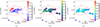 |
Fig. 4 Physical parameter maps of Field 3. (a) Centroid velocity map. (b) Velocity dispersion map. (c) Kinetic temperature map. The ellipses are the same as those in Fig. 2. |
Ranges of derived physical properties in each field.
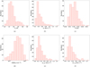 |
Fig. 5 Distributions of the physical parameters of NH3 fragments. (a) Histogram of kinetic temperatures Tk. (b) Histogram of total velocity dispersions συ (including bulk motions and using the thermal component of the entirety of the molecular gas). (c) Histogram of deconvolved radii of NH3 fragments Rdec. (d) Histogram of NH3 column density N(NH3). (e) Histogram of nonthermal velocity dispersion with bulk motions συ,NT. (f) Histogram of nonthermal velocity dispersion without bulk motions συ,ng. |
Statistics of physical parameters of NH3 fragments.
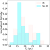 |
Fig. 6 Histogram of average kinetic temperatures of the NH3 fragments coinciding with the condensations of 1.3 mm continuum emission. Those matched with IR sources are colored in red, while the rest are colored in cyan. |
5 Discussion
5.1 Morphology
5.1.1 Comparison between ammonia observations and H2 column density
The NH3 (1,1) emissions in our data show diverse morphologies in the moment-0 maps, such as filaments (Field 28), core-like structures (Field 6), hub-like structures (Field 13), and dispersed features (Field 17). The morphology of the NH3 (1,1) emission can be affected by protostellar feedback during core evolution. During the star formation process, increasing feedback from protostars can distort their envelopes (Motte et al. 2018) and heat the surrounding gas. The NH3 (1,1) line gets much weaker and becomes undetectable when the gas temperature rises beyond 100 K (Ho & Townes 1983). Therefore, the morphology of the NH3 in MDCs could evolve from a concentrated distribution at the peak of the H2 density profile (hereafter, the M1 stage) to a dispersed shape around the protostar (hereafter, M2), and finally become undetectable (hereafter, M3). In order to construct an evolutionary sequence of the MDCs in Cygnus X, we compared the morphology of the NH3 (1,1) emission to that of the H2 column density (from the column density map, hereafter N-map, derived from spectral energy distribution (SED) fitting in Cao et al. 2019) of the MDCs, and classified the MDCs with infrared emissions. We present our findings in the following subsection.
As shown in Fig. 8 and Appendix C, the NH3 (1,1) emission is strongly correlated with dense regions of the N-map in most fields, indicating that the NH3 (1,1) line emission generally traces the dense structures in molecular gas. Nevertheless, the difference in resolution (~3″.1 for NH3 data and ~20″ for the N-map) leads to a more complicated morphology of NH3 (1,1) emission than that of the N-map for our MDCs. We also find that many of the peaks of the NH3 (1,1) emission show slight offsets from the peaks in the N-map, which could result from the depletion of NH3 around protostars (Tobin et al. 2011; Sewilo et al. 2017) and from the difference in resolution between the N-map and the NH3 cubes.
In light of their morphologies, we find that most (27 out of 35) MDCs are at the M1 stage. This result is consistent with our expectations, because the majority of our MDCs are not very evolved. As for the MDCs at the M2 stage (8 out of 35), we find evident star-forming activity (radio continuum emission, water masers, or bright sources on Spitɀer images) in all of them, which corroborates the mentioned mechanism for distorted NH3 (1,1) morphology. The MDCs at the M3 stage are not included in Table 6 because of their nondetection with the NH3 (1,1) line. Figures 8 and 9 present some example MDCs in each stage.
5.1.2 A possible evolutionary sequence in our sample
The evolution of MDCs is a fundamental piece in our understanding of high-mass star formation. There have been many studies focusing on this topic, both observational and theoretical (e.g., Chambers et al. 2009; Battersby et al. 2014b; Molinari et al. 2019). Based on theoretical frameworks and observations, a simple four-stage evolutionary scenario of MDCs is proposed as CDMC→HDMC→DAMS→FIMS by Zinnecker & Yorke (2007), where CDMC, HDMC, DAMS and FIMS stand for cold dense massive core, hot dense massive core, disk-accreting main sequence star, and final main sequence star, respectively. Recently, Motte et al. (2018) updated the star-formation pictures in different scales: (1) at the scale of 1–10 pc, the gas is fed into clumps by the inflow on ridges and hubs; (2) at the scale of ~0.1 pc, the beginning of star-forming activity will make starless MDCs grow into protostellar MDCs; (3) the stellar embryos in high-mass protostars grow from low-mass ones into high-mass ones, which transform the high-mass protostars from IR-quiet into IR-bright at ~0.02 pc scales; and (4) the HII region phase at 0.01–10 pc scales is the end of this scenario.
Although the evolution of high-mass protostars cannot be properly determined based on their infrared SEDs – as is possible for the low-mass ones – due to their complicated environments (Andre et al. 1993; Marseille et al. 2010), the infrared properties can still serve as an indicator of the evolution of embedded high-mass protostars. In order to obtain a better estimation of evolutionary stage, we adopt the infrared classification of Wang et al. (2022)5. The MDCs are divided into three groups: 8 IR-bright MDCs, 25 IR-quiet MDCs, and 2 starless MDCs. The IR-bright MDCs correspond to MDCs with possible embedded high-mass protostar(s), while the IR-quiet ones only harbor low-mass protostars. Regarding the MDCs without any star-forming activity according to the criterion of Wang et al. (2022), we take them as starless MDC candidates. To illustrate the evolutionary stages of MDCs, we combine the data at hand, which include NH3 emission data, the N-map, water masers, radio continuum sources, and mid-infrared pseudo three-color maps (8, 4.5, and 3.6 µm emission colored in red, green, and blue, respectively), into a composite image for each field (see Figs. 8 and 9).
Figure 8 shows three MDCs at the M1 stage. The MDC 774 and 1179 are the only two starless MDCs in our sample. In the IR-quiet MDC 1225, we find two radio sources and two water masers, indicating star-forming activities and the existence of protostar(s). As the protostar or protostars grow, stronger feedback distorts the morphology of NH3, which could be the situation shown in Fig. 9. The MDC 725 and 1454 are considered to be at stage M2. The MDC 725 is an IR-bright MDC with a radio source; that is, the high-mass stellar embryo or embryos have formed in it, while the MDC 1454 is an IR-quiet MDC with NH3 (1,1) emission distorted near the density peak. The MDC 1201 and 675 illustrate the latest stages in our sample, where most of the NH3 is destroyed and NH3 (1,1) emission is almost undetected within them. The MDC 1201 and 675 are IR-bright and IR-quiet, respectively. In conclusion, the morphology of the NH3 (1,1) emission could be a possible indicator for the evolutionary stage of MDCs.
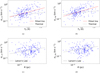 |
Fig. 7 Correlations between physical parameters of NH3 fragments. Panels a and b plot nonthermal velocity dispersions including or excluding the bulk motions versus kinetic temperature. The red and gray lines show the fitted result of the linear regression and the thermal velocity dispersion. There are positive correlations in both of them. Panels c and d plot nonthermal velocity dispersions including or excluding the bulk motions versus deconvolved radius. The gray line shows Larson’s law. |
5.2 Virial analysis
The virial parameter, which is the ratio between the kinetic energy and the gravitational energy, is an important indicator of the dynamical conditions of molecular structures, especially for those in early evolutionary stages. Typically, the turbulent core accretion model requires a virialized MDC as the birth place of the high-mass star (McKee & Tan 2002). Previous studies in which a virial analysis was carried out using different gas tracers at different size scales found that the distribution of virial parameters varies greatly with the sizes of molecular structures (e.g., Larson 1981; Heyer et al. 2001; Chen et al. 2019). The virial parameters of molecular clouds (~ 10 pc) are mostly ≫2, which is the critical value of an isothermal sphere in hydrostatic equilibrium embedded in a pressurized medium (Bonnor 1956; Ebert 1955; Larson 1981), while virial (1 ≤ αvir ≤ 2) and subvirial structures (αvir < 1) are found in the fragments (~0.01–1 pc) within molecular clouds (e.g., Pillai et al. 2011; Li et al. 2013). In this section, we perform a virial analysis of MDCs and try to understand their stability.
5.2.1 Calculation of virial parameters
As defined in Bertoldi & McKee (1992), the virial parameter, αvir, is in the form of
 (12)
(12)
where συ is the velocity dispersion and R is the radius of the structure. In this work, the total velocity dispersion of the whole molecular gas, συ, is obtained from the NH3 results, and the mass of MDCs is provided by Cao et al. (2021). We therefore calculate the virial parameters for MDCs that have both NH3 (1,1) and (2,2) detections. It is worth noting that we include the contributions from both turbulence and kinematics in the calculation of συ. Detailed calculation processes are listed in Appendix E.
In many MDCs, the detected NH3 emission only covers part of the spatial extent of MDCs (such as the MDC 725 in Fig. 9). For these cases, we take the sizes of their detected parts, Rsel, and calculate the corresponding mass, Msel, by multiplying their areas by the column densities taken from the N-map. Using Rsel and Msel, the virial parameters are calculated for the detected parts of the MDCs, which are called “partial” virial parameters in our analysis. The partial virial parameters are considered to be an upper limit value for their host MDCs. Such overestimation comes from two aspects, R/M and συ. First, we compare Rsel/Msel of the selected parts and Rtotal/Mtotal of their host MDCs. Figure 10 shows that all the ratios between Rsel/Msel and Rtotal/Mtotal are larger than 1, suggesting R/M is overestimated in the partial virial parameters. Second, as shown in Appendices A and B, the velocity dispersion is usually enhanced where the integral NH3 (1,1) emission is strong in most sources. The undetected parts should therefore have lower velocity dispersion than the detected parts, indicating the velocity dispersion is also overestimated in the partial virial parameters.
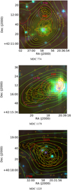 |
Fig. 8 MDCs at the Ml stage (i.e., the NH3 (1,1) emission is roughly concentrated around the column density peaks). The background is pseudo three-color images of each field, with Spitɀer 8, 4.5, and 3.6 µm emission colored in red, green, and blue, respectively. The contours of H2 column density and NH3 (1,1) integrated emission are over-plotted with green and orange, respectively. Cyan and magenta crosses mark the positions of any H2O masers or radio continuum sources, respectively. The starless, IR-quiet, and IR-bright MDCs are shown as pink dashed, red dashed, and red solid ellipses, respectively. More figures are showed in Appendix C. |
5.2.2 Distribution of virial parameters
Through the above calculations, we determined the virial parameters for 35 MDCs, including 14 full ones and 21 partial ones, as listed in Table 6. The mean and median values of the virial parameter are 1.0 and 0.9, respectively, with a standard deviation of 1.0. The majority of MDCs (23 out of 35) have a virial parameter of smaller than 1. Moreover, most full virial parameters (11 out of 14) are smaller than 1, with only one exceeding 2. Furthermore, the partial virial parameters, mostly distributed around 1, are considered as upper limits in our analysis, indicating that the majority of MDCs could be subvirialized. This result is consistent with previous findings that many MDCs are moderately to strongly subvirial (e.g., Pillai et al. 2011; Wienen et al. 2012; Li et al. 2013, 2020; Lu et al. 2014; Keown et al. 2017; Kerr et al. 2019; Traficante et al. 2020; Zhang et al. 2015; Ohashi et al. 2016). Recently, Singh et al. (2021) proposed three possible sources of bias that could result in a false subvirial result when calculating virial parameters: neglected bulk motions, an overestimated density profile correction factor, and mass contribution from the fore- and/or background. We tried to exclude these sources of bias in our calculation: (1) The bulk motions are considered in the total kinetic energy of MDCs; (2) the density profile correction factor is taken as 1 as defined in Singh et al. (2021), which could result in an overestimated virial parameter rather than an underestimated one; and (3) the mass of our MDCs is derived from the SED fitting results of Cao et al. (2019), where the fore- and background are removed in the fitting processes. Our subvirial results should therefore not be affected by these sources of bias and we consider them to be trustworthy.
As a result, our MDCs appear to be mostly subvirialized, which is not expected based on the turbulence core accretion model (McKee & Tan 2002). This suggests that MDCs could undergo dynamical collapse in nonequilibrium in the early stages of star formation unless there is additional support. Regarding high-mass star formation, the subvirial prestellar cores, according to the simulation work by Rosen et al. (2019), are more likely to form massive stars than virialized ones due to their higher accretion rates and lower levels of fragmentation. Additionally, an anti-correlation between the virial parameter and mass has been found in many works using only a single gas tracer (e.g., Lada et al. 2008; Foster et al. 2009). We also plot virial parameter versus mass for our sample of MDCs in Fig. 11. However, the Pearson’s correlation coefficient of the fitted line is only 0.18, which indicates no correlation. This is mainly due to the fact that the mass range of the MDCs in our sample is very small compared with other works (e.g., Roman-Duval et al. 2010; Wienen et al. 2012), namely ~101−102 M⊙. This trend also disappears in the combination of works with different gas tracers and different samples (Kauffmann et al. 2013). Traficante et al. (2018) interpret this trend as an observational bias due to the limitation of gas tracers.
As mentioned above, the subvirial MDCs would collapse if there were no additional support. Previous studies suggested that the magnetic field could provide significant support in MDCs (e.g., Frau et al. 2014; Hull & Zhang 2019; Liu et al. 2020, 2022). Following the methods in Liu et al. (2020), the total virial mass – which includes the contribution of magnetic field – can be calculated as
 (13)
(13)
where Mk = αvirM is the kinetic virial mass, and MB here is
 (14)
(14)
We then calculated the total virial parameter, αk+B = Mk+b/M, by assuming a typical magnetic field strength of ~0.5 mG (Hezareh et al. 2014). The results are shown in Fig. 12 for comparison with the original results in Fig. 11.
The mean and median values of the total virial parameter are 2.2 and 2.1, with a standard deviation of 1.2. The majority of total virial parameters are approximately 2 (as shown in Kauffmann et al. 2013, the critical virial parameter is ~2 for Bonnor-Ebert spheres), indicating that most MDCs are expected to be in stability with a typical magnetic field strength of 0.5 mG. In addition, if there is a strong magnetic field strength up to 1 mG, the total virial parameter would increase by ~ 1–2 in value. In addition, Liu et al. (2022) find an anti-correlation between the magnetic virial parameter (αB = MB /M) and the column density of H2. Considering the typical column density of our MDCs, of namely ~1023 cm−3, the magnetic virial parameters are ~0.5 in Liu et al. (2022), indicating that the magnetic field could provide remarkable support against the gravity. In our results, the non-thermal velocity dispersion of MDCs is lower than that predicted by McKee & Tan (2002), ~1.65(m/30M⊙)1/4Σ1/4 km s−1. Subsequent studies using this model (e.g., Krumholz & McKee 2005) also proposed significant support from the magnetic field against the gravity at the scale of MDCs. The Cygnus X North and South regions are also covered by the lower resolution NH3 survey (KEYSTONE) presented in Keown et al. (2019). The virial parameter of the NH3 cores presented by these authors (≳ 0.1 pc, referring to the NH3 “leaves” in that paper) show higher values than our results. A significant part of the NH3 cores are at supervirial states in Keown et al. (2019). Therefore, the parent structures of our NH3 fragments have larger virial parameters, indicating that the accretion of “cores” may not be dominated by the gravity. The gas might be fed to the “core” via the filament or the initial inflow suggested by Motte et al. (2018) and Padoan et al. (2020).
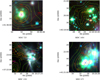 |
Fig. 9 MDCs at the M2 stage (MDC 725 and 1454) and M3 stage (MDC 1201 and 675). Marks are the same as those in Fig. 8. For MDC 1201, there is nearly no NH3 (1,1) emission in it. As for MDC 675, NH3 (1,1) emission is only detected in a few isolated beams around the density peak. We therefore consider both of them to be MDCs at the M3 stage. |
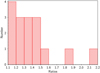 |
Fig. 10 Distribution of the ratios between Rsel/Msel and Rtotal/Mtotal. |
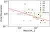 |
Fig. 11 Virial parameters vs. mass of the 35 MDCs in Cygnus X. In the legends, “B”, “Q”, and “S” refer to different infrared classes, IR-bright, IR-quiet, and starless, respectively. “F” and “N” are the same as those in Table 6. The red line shows the least-linear-square fitting result. The gray dashed lines show where virial parameters are equal to 1 and 2. |
5.3 Dynamical states in star-forming regions
We produced nonthermal velocity dispersion maps of each field and mark the regions where the nonthermal velocity dispersion is higher than the sound speed with green contours (Fig. 13). We find the dynamical states vary among different MDCs. As shown in Fig. 13, the MDC 248 is dominated by the transsonic to supersonic nonthermal velocity dispersion (𝓜NT ≥ 1), while the nonthermal velocity dispersion in MDC 892 is almost entirely subsonic. The majority of MDCs consist of both supersonic and subsonic regions, such as MDCs 274, 584, and 774. Maps of other fields are reported in Appendix D.
In Sect. 4.2, we provide the συ,NT and συ,ng of NH3 fragments, where the resolved bulk motions are included and excluded, respectively. We also calculate συ,NT and συ,ng for MDCs. Then, using συ,NT and συ,ng, we obtain the Mach numbers, 𝓜NT and 𝓜ng, for both NH3 fragments and MDCs (Fig. 14). For MDCs, 𝓜NT has mean and median values of 2.2 and 2.3, with a standard deviation of 0.8, while the mean and median values of 𝓜ng are 1.9 and 1.9, with a standard deviation of 0.7. As for NH3 fragments, the majority of both 𝓜NT and 𝓜ng are smaller than 2 (trans-sonic to subsonic). The mean and median values of 𝓜NT are 1.4 and 1.2, with a standard deviation of 0.8, and the mean and median values of 𝓜ng are 1.3 and 1.1, with a standard deviation of 0.7. These distributions of NH3 fragments are similar to previous results (e.g., Sokolov et al. 2018; Yue et al. 2021; Li et al. 2020) The differences between 𝓜NT and 𝓜ng of MDCs are more remarkable than those of NH3 fragments, suggesting that the bulk motions have a larger contribution to the nonthermal velocity dispersions of MDCs than those of NH3 fragments. In contrast, the 𝓜ng and 𝓜NT of NH3 fragments are close. Moreover, both panels show a decreasing trend in Mach number from MDCs to NH3 fragments.
Recently, high-spatial-resolution observations revealed similar transonic and subsonic nonthermal velocity dispersion in both low-mass and high-mass star-forming regions, such as L1517 (Hacar & Tafalla 2011), NGC 1333 (Hacar et al. 2017), the Orion integral filament (Hacar et al. 2018), OMC 2/3 (Yue et al. 2021), and NGC 6334S (Li et al. 2020). Comparing N2H+ J = 1 − 0 observations from the Nobeyama 45m telescope and ALMA, Yue et al. (2021) propose the nonthermal motions would transit from supersonic motions to subsonic motions at a scale of ~0.05 pc. In our results, the transition occurs at a scale of NH3 fragments, ~0.04 pc, which is consistent with the result of Yue et al. (2021). These latter authors interpret this transition as a resolution-dependent bias, where more bulk motions are involved in larger beams and give a greater nonthermal velocity dispersion. The large-scale dispersion measured from Nobeyama observations, σls, is decomposed in Yue et al. (2021) into small-scale dispersion measured from ALMA observations, σss, bulk motion probed by dispersion between the peak velocity of each ALMA beam, σbm, and residual dispersion, σrd, with the relation  . Comparing 𝓜ng of MDCs with that of NH3 fragments as shown in the panel b of Fig. 14, where the bulk motions are deducted, the decreasing trend of 𝓜ng from MDCs to NH3 fragments still remains. The differences between the 𝓜ng of MDCs and that of NH3 fragments could refer to σrd. A possible explanation for σrd is turbulent vortex, as put forward by Yue et al. (2021). In most cases, the decrease in nonthermal velocity dispersion from large scale to small scale is also thought to be the dissipation of turbulence, as suggested by the relation between velocity dispersion and size at lower spatial resolutions (~0.1–100 pc) in Larson (1981). Considering that the typical size of NH3 fragments (~0.04 pc is larger than the typical Kolmogorov scale in molecular clouds (~10−5–10−4 pc; McKee & Ostriker 2007; Kritsuk et al. 2011; Qian et al. 2018), the turbulent dissipation could be a possible cause for the decreasing trend of 𝓜ng.
Furthermore, the lower Mach numbers imply that magnetic fields can play a more important role if the fragments are in a virialized state. However, as shown in Liu et al. (2022), αB would decrease with increasing column density. Considering that αB is about 0.5 in our MDCs, the gravity could be more dominant than the magnetic field in these fragments (usually the peaks on the column density map). As estimated by Sokolov et al. (2018), magnetic fields with strengths over ~ 1 mG are needed to achieve virialization in these fragments. However, such a strong magnetic fields have only been detected in a small number of star-forming structures (e.g., Curran & Chrysostomou 2007; Fish & Sjouwerman 2007; Palau et al. 2021). Therefore, the fragments of MDCs are probably not in virialized states.
Properties of MDCs with NH3 detection.
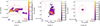 |
Fig. 13 Nonthermal velocity dispersion maps of Fields 3, 5, and 26. The green contours show the regions with Mach numbers of greater than 1. The ellipses are the same as those in Fig. 2. |
5.4 Gas and dust temperature
In general, there are two ways to trace the temperature of molecular clouds: from the dust continuum emission or from spectral line emission of a certain molecule. As the temperatures of MDCs are also provided in Cao et al. (2021; Tdust column in Table 6), which were calculated from the SED fitting of the dust continuum data, we compared these temperatures with the temperatures derived from the NH3 data; we present our findings below.
In order to compare the NH3 temperature and the dust temperature in MDCs, the NH3 data cubes are convolved to the resolution of temperature map in Cao et al. (2019) and the NH3 temperatures of MDCs are rederived (Tgas column in Table 6). The correlation between them is plotted in Fig. 15. The gray line illustrates where Tgas = Tdust and the red line presents the linear regression fitting result,
 (15)
(15)
with the correlation coefficient r = 0.66. According to this relation, the gas temperature is mostly higher than the dust temperature when Tgas ≳ 20 K. In the scatter plot, the turning point is also around 20 K. We find that Tdust is almost equal to Tgas when Tgas ≲ 20 K and deviates from Tgas when Tgas ≳ 20 K.
The gas and dust are expected to be well coupled – that is, they can be characterized by the same temperature – within a molecular core with a density of ≳ 104.5 cm−3 (Goldsmith 2001; Young et al. 2004). This coupling has been confirmed by many works (e.g., Dunham et al. 2010; Merello et al. 2019). However, although all the MDCs in our sample have densities higher than 105 cm−3 , Tgas and Tdust are not thermally well coupled. Similarly, in high-mass star-forming regions, Tgas is usually measured to be higher than Tdust, which is the case for example for the quiescent clumps in Battersby et al. (2014a), the S 140 in Koumpia et al. (2015), and the W40 in Tursun et al. (2020).
The origin of the excess gas temperature is a complex open question. In the photon-dominated region S 140, Koumpia et al. (2015) found an excess of ~5–15 K in their deeply embedded regions, where Tdust and Tgas are expected to be well coupled in the KOSMA-τ PDR model (Röllig et al. 2013). Koumpia et al. (2015) interpret these differences as the result of inhomogeneous clumpy structures, which could lead to a deeper penetration of the UV radiation and heating of the gas in the embedded cores. In addition, differences between Tgas and Tdust can also arise from different layers traced by the gas and the dust (Battersby et al. 2014a). Such differences arise from both different excitation conditions and different angular resolutions. The NH3 (1,1) and (2,2) lines are usually excited in the dense gas, while the dust continuum emission arises from a range of densities. In the present work, the resolutions of the NH3 data and the temperature map from Cao et al. (2019) are quite different. Only a few MDCs have sufficient temperature pixels as shown in Fig. 4 and Appendix B. The spatially extended NH3 emission, which usually has lower temperatures, is missed due to the filtering effect of VLA. In our results, Tgas deviates from Tdust at Tgas ≳ 20 K (Fig. 15). The MDCs with Tgas ≳ 20 K should have internal heating from the star-forming activity, but this heating is diluted by the large beam in the dust temperature data. Therefore, on average, we obtain a higher Tgas than Tdust in our results.
6 Summary
The initial conditions of the birth places of high-mass stars are of utmost importance in the study of high-mass star formation. We present VLA NH3 (1,1) and (2,2) observations of MDCs in Cygnus X at a distance of 1.4 kpc. As a part of the CENSUS project, we provide the temperature and dynamical information derived from the simultaneous line fitting of the NH3 (1,1) and (2,2) inversion emission lines.
We used the MDCs catalog from Cao et al. (2021) in our analysis. We compared the morphology between the H2 column density map from Cao et al. (2019) and NH3 (1,1) emission within each MDC and provide a possible indicator for estimating their evolutionary stages. We also performed a virial analysis for each MDC to evaluate the stability of the MDCs. The dynamical states of the MDCs are discussed based on their nonthermal velocity dispersions. We also compare the gas temperature with the dust temperature of MDCs. In addition, we identified 202 fragments from the NH3 (1,1) moment-0 maps using the GAUSS-CLUMPS algorithm. We derived the physical parameters of these NH3 fragments and conducted a correlation analysis among them. We also analyzed the dynamical states of the NH3 fragments and compared them with those of the MDCs. The main results of this paper can be summarized as follows:
The NH3 fragments have a mean deconvolved radius of 0.02 pc, a mean velocity dispersion of 0.46 km s−1, a mean nonthermal velocity dispersion of 0.37 km s−1, a mean kinetic temperature of 18.6 K, and a mean NH3 column density of 3.9 × 1015 cm−2. Comparison with the temperature of structures in previous works indicates that the NH3 fragments are mostly early evolved structures;
We find a correlation between nonthermal velocity dispersion and kinetic temperature. This correlation is likely the result of different levels of star-forming activity. A molecular structure with more active star-forming activity is usually hotter and with larger velocity dispersion;
We perform a morphological analysis of the NH3 (1,1) emission and column density map of MDCs. We propose a possible evolutionary sequence of MDCs based on the NH3 (1,1) emission: in the early, relatively little-evolved MDCs, the NH3 emission is concentrated around density peaks; the NH3 emission is subsequently dispersed by the star-forming activity, after which, in the evolved MDC, the NH3 emission becomes undetected;
We perform a virial analysis of all MDCs. The majority of the MDCs of our sample are subvirialized, indicating that the kinetic energy cannot support the MDCs alone in our sample. Considering the support from magnetic fields, MDCs could attain their stability states if there were a typical magnetic field strength of ~0.5 mG;
We investigate the dynamic states of MDCs and the NH3 fragments with their nonthermal Mach numbers. The Mach numbers show a decreasing trend from MDCs to NH3 fragments, which could be an indication of the dissipation of turbulence. When the resolved bulk motions are excluded from the nonthermal velocity dispersion, we find the NH3 fragments are mostly subsonic to trans-sonic, while the majority of MDCs are transonic;
The gas temperature derived from NH3 (1,1) and (2,2) lines is compared with the dust temperature calculated by SED fitting from Cao et al. (2019). The two are well coupled when the gas temperature is ≲ 20 K, while the gas temperature is mostly larger than the dust temperature when the gas temperature is ≳20 K.
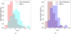 |
Fig. 14 Normalized density distribution of 𝓜NT and 𝓜ng in NH3 fragments and MDCs. The contribution of velocity gradient is included in (a) and excluded in (b). |
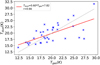 |
Fig. 15 Correlation between Tgas and Tdust. The red line shows the linear regression fitting results, and the gray line shows where Tdust = Tgas. |
Acknowledgements
This work is supported by National Key R&D Program of China No. 2022YFA1603103, No. 2017YFA0402604, the National Natural Science Foundation of China (NSFC) grant U1731237, and the science research grant from the China Manned Space Project with no. CMS-CSST-2021-B06. This research made use of APLpy, an open-source plotting package for Python. (Robitaille & Bressert 2012) This research made use of Astropy, a community-developed core Python package for Astronomy (Astropy Collaboration 2013, 2018). This study used observations from the Spitzer Space Telescope Cygnus X Legacy Survey (PID 40184, P.I. Joseph L. Hora).
Appendix A Overview of observations of detected spectral lines
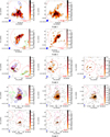 |
Fig. A.1 Moment-0 maps with remarkable detection of NH3 (J,K) = (1,1), (2,2), (3,3), (4,4), and (5,5) inversion lines among our observations. The (1,1) maps are plotted from a 3 rms level and in steps of 2σ, while others are plotted from the 2 rms level and in steps of 2σ. The IR-bright, IR-quiet, and starless MDCs are shown as red solid, red dashed, and pink dashed ellipses, respectively. The smaller ellipses present the fragments extracted using the GAUSSCLUMPS algorithm. The blue ones are included in the parameter analysis while the green ones are not. |
Appendix B Distributions of kinetic temperature, centroid velocity and velocity dispersion
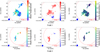 |
Fig. B.1 Distributions of kinetic temperature (left panel), centroid velocity (middle panel), and velocity dispersion (right panel) derived from the simultaneous fitting of NH3 (1,1) and (2,2) inversion lines. The ellipses are the same as those in Fig. A.1. |
Appendix C Compositive images
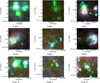 |
Fig. C.1 Compositive images of each field. The background is the Spitɀer three-color images using 8µm (R), 4.5µm (G), and 3.6µm (B) bands. The column density contours and NH3 (1,1) integrated emission contours are over-plotted with green and orange. Cyan and magenta crosses mark the positions of any H2O masers or radio continuum sources, respectively. The ellipses are the same as those in Fig. A.1. |
Appendix D Maps of non-thermal velocity dispersion
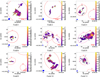 |
Fig. D.1 Nonthermal velocity dispersion maps of other fields. The green enclosing areas show the regions with Mach numbers larger than 1. The ellipses are the same as those in Fig. A.1. |
Appendix E Derivation of different velocity dispersions
There are three velocity dispersions used in our analyses of MDCs and NH3 fragments: the total velocity dispersion συ, the nonthermal velocity dispersion including the bulk motions συ,NT, and the nonthermal velocity dispersion excluding the bulk motions συ,ng.
First, for the total velocity dispersion, συ, both the velocity dispersion of a certain beam, συ,i·, and the gradient of υlsr need to be taken into account. The mean value of συ,i is calculated as root mean square (RMS) weighed by the integrated flux of the (1,1) line; that is,
 (E.1)
(E.1)
where w is the integrated flux of the NH3 (1,1) line from their moment-0 maps. The contribution of υlsr is derived as
![Mathematical equation: $\Delta {v_{{\rm{lsr}}}} = \sqrt {\Sigma \left[ {w \times {{\left( {{v_{{\rm{lsr}},i}} - \overline {{v_{{\rm{lsr}},i}}} } \right)}^2}} \right]/\Sigma (w)} ,$](/articles/aa/full_html/2024/04/aa45963-23/aa45963-23-eq27.png) (E.2)
(E.2)
where υlsr,i is the centroid velocity of a certain beam, and  is the weighted mean value υlsr,i. Here, συ is then derived as
 (E.3)
(E.3)
Generally, συ, including all the observed motions, is used in the virial analysis.
Similarly, συ,NT is calculated as the weighted RMS value from the nonthermal velocity dispersion maps combined with the contribution of υlsr, which is
 (E.4)
(E.4)
where συ,NTi is the nonthermal velocity dispersion of a certain beam.
In order to calculate συ,ng, we fit the bulk motions of υbm with a 2D linear function on the centroid velocity maps following the method provided in Goodman et al. (1993):
 (E.5)
(E.5)
where δα and δβ are the offsets in right ascension (RA) and declination (Dec). Then, the contribution of the bulk motion is estimated as
![Mathematical equation: $\Delta {v_{{\rm{bm}}}} = \sqrt {\Sigma \left[ {w \times {{\left( {{v_{{\rm{bm}},{\rm{i}}}} - \overline {{v_{{\rm{bm}}}}} } \right)}^2}} \right]/\Sigma (w)} ,$](/articles/aa/full_html/2024/04/aa45963-23/aa45963-23-eq32.png) (E.6)
(E.6)
where υbm,i is the fitted velocity of a certain beam. Deducting ∆υbm from συ,NT, we can obtain συ,ng as
 (E.7)
(E.7)
Both συ,NT and συ,ng are used in the calculation of the Mach numbers of different molecular structures.
References
- Andre, P., Ward-Thompson, D., & Barsony, M. 1993, ApJ, 406, 122 [NASA ADS] [CrossRef] [Google Scholar]
- Ao, Y., Henkel, C., Menten, K. M., et al. 2013, A&A, 550, A135 [NASA ADS] [CrossRef] [EDP Sciences] [Google Scholar]
- Astropy Collaboration (Robitaille, T. P., et al.) 2013, A&A, 558, A33 [NASA ADS] [CrossRef] [EDP Sciences] [Google Scholar]
- Astropy Collaboration (Price-Whelan, A. M., et al.) 2018, AJ, 156, 123 [Google Scholar]
- Barranco, J. A., & Goodman, A. A. 1998, ApJ, 504, 207 [Google Scholar]
- Battersby, C., Bally, J., Dunham, M., et al. 2014a, ApJ, 786, 116 [NASA ADS] [CrossRef] [Google Scholar]
- Battersby, C., Ginsburg, A., Bally, J., et al. 2014b, ApJ, 787, 113 [NASA ADS] [CrossRef] [Google Scholar]
- Berry, D. S., Reinhold, K., Jenness, T., & Economou, F. 2007, in ASP Conf. Ser., 376, Astronomical Data Analysis Software and Systems XVI, eds. R. A. Shaw, F. Hill, & D. J. Bell, 425 [NASA ADS] [Google Scholar]
- Bertoldi, F., & McKee, C. F. 1992, ApJ, 395, 140 [NASA ADS] [CrossRef] [Google Scholar]
- Beuther, H., Schilke, P., Menten, K. M., et al. 2002, ApJ, 566, 945 [Google Scholar]
- Billington, S. J., Urquhart, J. S., Figura, C., Eden, D. J., & Moore, T. J. T. 2019, MNRAS, 483, 3146 [NASA ADS] [CrossRef] [Google Scholar]
- Bonnell, I. A., Bate, M. R., Clarke, C. J., & Pringle, J. E. 1997, MNRAS, 285, 201 [NASA ADS] [CrossRef] [Google Scholar]
- Bonnell, I. A., Bate, M. R., & Zinnecker, H. 1998, MNRAS, 298, 93 [Google Scholar]
- Bonnell, I. A., Bate, M. R., Clarke, C. J., & Pringle, J. E. 2001, MNRAS, 323, 785 [Google Scholar]
- Bonnor, W. B. 1956, MNRAS, 116, 351 [NASA ADS] [CrossRef] [Google Scholar]
- Cao, Y., Qiu, K., Zhang, Q., et al. 2019, ApJS, 241, 1 [Google Scholar]
- Cao, Y., Qiu, K., Zhang, Q., Wang, Y., & Xiao, Y. 2021, ApJ, 918, L4 [NASA ADS] [CrossRef] [Google Scholar]
- Chambers, E. T., Jackson, J. M., Rathborne, J. M., & Simon, R. 2009, ApJS, 181, 360 [NASA ADS] [CrossRef] [Google Scholar]
- Chen, H.-R. V., Zhang, Q., Wright, M. C. H., et al. 2019, ApJ, 875, 24 [Google Scholar]
- Chira, R. A., Beuther, H., Linz, H., et al. 2013, A&A, 552, A40 [NASA ADS] [CrossRef] [EDP Sciences] [Google Scholar]
- Curran, R. L., & Chrysostomou, A. 2007, MNRAS, 382, 699 [NASA ADS] [CrossRef] [Google Scholar]
- Currie, M. J., Berry, D. S., Jenness, T., et al. 2014, in ASP Conf. Ser., 485, Astronomical Data Analysis Software and Systems XXIII, eds. N. Manset, & P. Forshay, 391 [NASA ADS] [Google Scholar]
- Dunham, M. K., Rosolowsky, E., Evans, Neal J., I., et al. 2010, ApJ, 717, 1157 [NASA ADS] [CrossRef] [Google Scholar]
- Ebert R. 1955 ZAp 37 217 [NASA ADS] [Google Scholar]
- Fish, V. L., & Sjouwerman, L. O. 2007, ApJ, 668, 331 [CrossRef] [Google Scholar]
- Foster, J. B., Rosolowsky, E. W., Kauffmann, J., et al. 2009, ApJ, 696, 298 [Google Scholar]
- Frau, P., Girart, J. M., Zhang, Q., & Rao, R. 2014, A&A, 567, A116 [NASA ADS] [CrossRef] [EDP Sciences] [Google Scholar]
- Ginsburg, A., Henkel, C., Ao, Y., et al. 2016, A&A, 586, A50 [NASA ADS] [CrossRef] [EDP Sciences] [Google Scholar]
- Goldsmith, P. F. 2001, ApJ, 557, 736 [Google Scholar]
- Goodman, A. A., Benson, P. J., Fuller, G. A., & Myers, P. C. 1993, ApJ, 406, 528 [Google Scholar]
- Gottschalk, M., Kothes, R., Matthews, H. E., Land ecker, T. L., & Dent, W. R. F. 2012, A&A, 541, A79 [NASA ADS] [CrossRef] [EDP Sciences] [Google Scholar]
- Guesten, R., Walmsley, C. M., Ungerechts, H., & Churchwell, E. 1985, A&A, 142, 381 [NASA ADS] [Google Scholar]
- Hacar, A., & Tafalla, M. 2011, A&A, 533, A34 [NASA ADS] [CrossRef] [EDP Sciences] [Google Scholar]
- Hacar, A., Tafalla, M., & Alves, J. 2017, A&A, 606, A123 [NASA ADS] [CrossRef] [EDP Sciences] [Google Scholar]
- Hacar, A., Tafalla, M., Forbrich, J., et al. 2018, A&A, 610, A77 [NASA ADS] [CrossRef] [EDP Sciences] [Google Scholar]
- Heyer, M. H., Carpenter, J. M., & Snell, R. L. 2001, ApJ, 551, 852 [NASA ADS] [CrossRef] [Google Scholar]
- Hezareh, T., Csengeri, T., Houde, M., Herpin, F., & Bontemps, S. 2014, MNRAS, 438, 663 [NASA ADS] [CrossRef] [Google Scholar]
- Ho, P. T. P., & Townes, C. H. 1983, ARA&A, 21, 239 [NASA ADS] [CrossRef] [Google Scholar]
- Hull, C. L. H., & Zhang, Q. 2019, Front. Astron. Space Sci., 6, 3 [Google Scholar]
- Immer, K., Kauffmann, J., Pillai, T., Ginsburg, A., & Menten, K. M. 2016, A&A, 595, A94 [NASA ADS] [CrossRef] [EDP Sciences] [Google Scholar]
- Jijina, J., Myers, P. C., & Adams, F. C. 1999, ApJS, 125, 161 [Google Scholar]
- Kauffmann, J., Bertoldi, F., Bourke, T. L., Evans, N. J., I., & Lee, C. W. 2008, A&A, 487, 993 [NASA ADS] [CrossRef] [EDP Sciences] [Google Scholar]
- Kauffmann, J., Pillai, T., & Goldsmith, P. F. 2013, ApJ, 779, 185 [NASA ADS] [CrossRef] [Google Scholar]
- Keown, J., Di Francesco, J., Kirk, H., et al. 2017, ApJ, 850, 3 [NASA ADS] [CrossRef] [Google Scholar]
- Keown J. Di Francesco J. Rosolowsky E. et al. 2019 ApJ 884 4 [NASA ADS] [CrossRef] [Google Scholar]
- Kerr, R., Kirk, H., Di Francesco, J., et al. 2019, ApJ, 874, 147 [NASA ADS] [CrossRef] [Google Scholar]
- Koumpia, E., Harvey, P. M., Ossenkopf, V., et al. 2015, A&A, 580, A68 [NASA ADS] [CrossRef] [EDP Sciences] [Google Scholar]
- Kraemer, K. E., Hora, J. L., Adams, J., et al. 2010, in Am. Astron. Soc. Meeting Abstracts, 215, American Astronomical Society Meeting Abstracts #215, 414.01 [NASA ADS] [Google Scholar]
- Kritsuk, A. G., Nordlund, Å., Collins, D., et al. 2011, ApJ, 737, 13 [NASA ADS] [CrossRef] [Google Scholar]
- Krumholz, M. R. 2015, arXiv e-prints, [arXiv:1511.03457] [Google Scholar]
- Krumholz, M. R. & McKee, C. F. 2005, ApJ, 630, 250 [NASA ADS] [CrossRef] [Google Scholar]
- Lada, C. J., Muench, A. A., Rathborne, J., Alves, J. F., & Lombardi, M. 2008, ApJ, 672, 410 [Google Scholar]
- Larson, R. B. 1981, MNRAS, 194, 809 [Google Scholar]
- Leung, H. O., & Thaddeus, P. 1992, ApJS, 81, 267 [NASA ADS] [CrossRef] [Google Scholar]
- Li, D., Goldsmith, P. F., & Menten, K. 2003, ApJ, 587, 262 [NASA ADS] [CrossRef] [Google Scholar]
- Li, D., Kauffmann, J., Zhang, Q., & Chen, W. 2013, ApJ, 768, L5 [NASA ADS] [CrossRef] [Google Scholar]
- Li, S., Zhang, Q., Liu, H. B., et al. 2020, ApJ, 896, 110 [Google Scholar]
- Liu, J., Zhang, Q., Qiu, K., et al. 2020, ApJ, 895, 142 [Google Scholar]
- Liu, J., Qiu, K., & Zhang, Q. 2022, ApJ, 925, 30 [NASA ADS] [CrossRef] [Google Scholar]
- Lu, X., Zhang, Q., Liu, H. B., Wang, J., & Gu, Q. 2014, ApJ, 790, 84 [NASA ADS] [CrossRef] [Google Scholar]
- Mangum, J. G., & Shirley, Y. L. 2015, PASP, 127, 266 [Google Scholar]
- Marseille, M. G., van der Tak, F. F. S., Herpin, F., & Jacq, T. 2010, A&A, 522, A40 [NASA ADS] [CrossRef] [EDP Sciences] [Google Scholar]
- McKee, C. F., & Tan, J. C. 2002, Nature, 416, 59 [CrossRef] [Google Scholar]
- McKee, C. F., & Tan, J. C. 2003, ApJ, 585, 850 [Google Scholar]
- McKee, C. F., & Ostriker, E. C. 2007, ARA&A, 45, 565 [Google Scholar]
- McMullin, J. P., Waters, B., Schiebel, D., Young, W., & Golap, K. 2007, in ASP Conf. Ser., 376, Astronomical Data Analysis Software and Systems XVI, eds. R. A. Shaw, F. Hill, & D. J. Bell, 127 [NASA ADS] [Google Scholar]
- Merello, M., Molinari, S., Rygl, K. L. J., et al. 2019, MNRAS, 483, 5355 [NASA ADS] [CrossRef] [Google Scholar]
- Molinari, S., Baldeschi, A., Robitaille, T. P., et al. 2019, MNRAS, 486, 4508 [Google Scholar]
- Motte, F., Bontemps, S., Schilke, P., et al. 2007, A&A, 476, 1243 [NASA ADS] [CrossRef] [EDP Sciences] [Google Scholar]
- Motte, F., Bontemps, S., & Louvet, F. 2018, ARA&A, 56, 41 [NASA ADS] [CrossRef] [Google Scholar]
- Ohashi, S., Sanhueza, P., Chen, H.-R. V., et al. 2016, ApJ, 833, 209 [NASA ADS] [CrossRef] [Google Scholar]
- Ott, J., Henkel, C., Braatz, J. A., & Weiß, A. 2011, ApJ, 742, 95 [NASA ADS] [CrossRef] [Google Scholar]
- Padoan, P., Pan, L., Juvela, M., Haugbølle, T., & Nordlund, Å. 2020, ApJ, 900, 82 [NASA ADS] [CrossRef] [Google Scholar]
- Palau, A., Zhang, Q., Girart, J. M., et al. 2021, ApJ, 912, 159 [NASA ADS] [CrossRef] [Google Scholar]
- Pan, X., Qiu, K., Yang, K., Cao, Y., & Zhang, X. 2024, A&A, 684, A141 (Paper II) [NASA ADS] [CrossRef] [EDP Sciences] [Google Scholar]
- Pillai, T., Wyrowski, F., Carey, S. J., & Menten, K. M. 2006, A&A, 450, 569 [NASA ADS] [CrossRef] [EDP Sciences] [Google Scholar]
- Pillai, T., Kauffmann, J., Wyrowski, F., et al. 2011, A&A, 530, A118 [CrossRef] [EDP Sciences] [Google Scholar]
- Pokhrel, R., Myers, P. C., Dunham, M. M., et al. 2018, ApJ, 853, 5 [NASA ADS] [CrossRef] [Google Scholar]
- Qian, L., Li, D., Gao, Y., Xu, H., & Pan, Z. 2018, ApJ, 864, 116 [CrossRef] [Google Scholar]
- Rathborne, J. M., Whitaker, J. S., Jackson, J. M., et al. 2016, PASA, 33, e030 [NASA ADS] [CrossRef] [Google Scholar]
- Robitaille, T., & Bressert, E. 2012, Astrophysics Source Code Library [record ascl:1208.017] [Google Scholar]
- Röllig, M., Szczerba, R., Ossenkopf, V., & Glück, C. 2013, A&A, 549, A85 [Google Scholar]
- Roman-Duval, J., Jackson, J. M., Heyer, M., Rathborne, J., & Simon, R. 2010, ApJ, 723, 492 [NASA ADS] [CrossRef] [Google Scholar]
- Rosen, A. L., Li, P. S., Zhang, Q., & Burkhart, B. 2019, ApJ, 887, 108 [NASA ADS] [CrossRef] [Google Scholar]
- Rygl, K. L. J., Brunthaler, A., Sanna, A., et al. 2012, A&A, 539, A79 [NASA ADS] [CrossRef] [EDP Sciences] [Google Scholar]
- Sánchez-Monge, Á., Palau, A., Fontani, F., et al. 2013, MNRAS, 432, 3288 [CrossRef] [Google Scholar]
- Sewilo, M., Wiseman, J., Indebetouw, R., et al. 2017, ApJ, 849, 68 [CrossRef] [Google Scholar]
- Shu, F., Najita, J., Galli, D., Ostriker, E., & Lizano, S. 1993, in Protostars and Planets III, eds. E. H. Levy, & J. I. Lunine, 3 [Google Scholar]
- Singh, A., Matzner, C. D., Friesen, R. K., et al. 2021, ApJ, 922, 87 [CrossRef] [Google Scholar]
- Sokolov, V., Wang, K., Pineda, J. E., et al. 2018, A&A, 611, L3 [NASA ADS] [CrossRef] [EDP Sciences] [Google Scholar]
- Swift, J. J., Welch, W. J., & Di Francesco, J. 2005, ApJ, 620, 823 [NASA ADS] [CrossRef] [Google Scholar]
- Tafalla, M., Myers, P. C., Caselli, P., & Walmsley, C. M. 2004, A&A, 416, 191 [NASA ADS] [CrossRef] [EDP Sciences] [Google Scholar]
- Takekoshi, T., Fujita, S., Nishimura, A., et al. 2019, ApJ, 883, 156 [NASA ADS] [CrossRef] [Google Scholar]
- Tang, X. D., Henkel, C., Menten, K. M., et al. 2018, A&A, 609, A16 [NASA ADS] [CrossRef] [EDP Sciences] [Google Scholar]
- Tobin, J. J., Hartmann, L., Chiang, H.-F., et al. 2011, ApJ, 740, 45 [NASA ADS] [CrossRef] [Google Scholar]
- Traficante, A., Lee, Y. N., Hennebelle, P., et al. 2018, A&A, 619, A7 [NASA ADS] [CrossRef] [EDP Sciences] [Google Scholar]
- Traficante, A., Fuller, G. A., Duarte-Cabral, A., et al. 2020, MNRAS, 491, 4310 [Google Scholar]
- Tursun, K., Esimbek, J., Henkel, C., et al. 2020, A&A, 643, A178 [NASA ADS] [CrossRef] [EDP Sciences] [Google Scholar]
- Uyanıker, B., Fürst, E., Reich, W., Aschenbach, B., & Wielebinski, R. 2001, A&A, 371, 675 [NASA ADS] [CrossRef] [EDP Sciences] [Google Scholar]
- Wang, Y., Qiu, K., Cao, Y., et al. 2022, ApJ, 927, 185 [NASA ADS] [CrossRef] [Google Scholar]
- Wendker, H. J., Higgs, L. A., & Landecker, T. L. 1991, A&A, 241, 551 [Google Scholar]
- Wienen, M., Wyrowski, F., Schuller, F., et al. 2012, A&A, 544, A146 [NASA ADS] [CrossRef] [EDP Sciences] [Google Scholar]
- Wolfire, M. G., & Cassinelli, J. P. 1987, ApJ, 319, 850 [NASA ADS] [CrossRef] [Google Scholar]
- Wu, Y., Zhang, Q., Yu, W., et al. 2006, A&A, 450, 607 [NASA ADS] [CrossRef] [EDP Sciences] [Google Scholar]
- Wu, G., Qiu, K., Esimbek, J., et al. 2018, A&A, 616, A111 [NASA ADS] [CrossRef] [EDP Sciences] [Google Scholar]
- Yang, K., Qiu, K., & Pan, X. 2024, A&A, 684, A140 (Paper I) [NASA ADS] [CrossRef] [EDP Sciences] [Google Scholar]
- Young, K. E., Lee, J.-E., Evans, Neal J., I., Goldsmith, P. F., & Doty, S. D. 2004, ApJ, 614, 252 [Google Scholar]
- Yue, N.-N., Li, D., Zhang, Q.-Z., et al. 2021, Res. Astron. Astrophys., 21, 024 [CrossRef] [Google Scholar]
- Zhang, C.-P., Csengeri, T., Wyrowski, F., et al. 2019, A&A, 627, A85 [NASA ADS] [CrossRef] [EDP Sciences] [Google Scholar]
- Zhang, Q., Wang, K., Lu, X., & Jiménez-Serra, I. 2015, ApJ, 804, 141 [Google Scholar]
- Zhang, C.-P., Li, G.-X., Pillai, T., et al. 2020, A&A, 638, A105 [EDP Sciences] [Google Scholar]
- Zinnecker, H., & Yorke, H. W. 2007, ARA&A, 45, 481 [Google Scholar]
These sources were not included by Motte et al. (2007) as the OB2 region has a lower extinction while Motte et al. (2007) extracted sources from high-extinction regions.
The National Radio Astronomy Observatory is a facility of the National Science Foundation operated under cooperative agreement by Associated Universities, Inc.
The IR-bright and quiet MDCs are classified according to their Spitɀer 24 µm fluxes or MSX 21 µm fluxes when 24 µm data are saturated. The criteria are 23 Jy for 24 µm flux and 17 Jy for 21 µm flux. The starless candidates are selected from IR-quiet MDCs, which are not associated with any water maser, radio source, or IR sources in 2MASS, Spitzer, Herschel, and MSX catalogs.
All Tables
All Figures
|
Fig. 1 Example five-component-fitting results on NH3 (1,1) and (2,2) emission (pixel coordinate (142,131) in Field 3). Upper panel: original spectrum and the fitted result are colored in black and red, respectively. Lower panel: residual spectrum of this fitting result. |
| In the text | |
|
Fig. 2 (a) Moment-0 map of the NH3 (1,1) line for Field 3. The contour is plotted from 3σ level and in steps of 2σ. The red ellipses show the MDCs identified from the H2 column density map (resolution ~20″) by Cao et al. (2021), and the blue ellipses illustrate the fragments extracted using the GAUSSCLUMPS algorithm. The magenta boxes show the condensations identified from the SMA 1.3 mm continuum, (b) Moment-0 map of the NH3 (2,2) line for Field 3. The contour is plotted from 2σ level and in steps of 2σ. |
| In the text | |
|
Fig. 3 Histogram of the average optical depth of the main component of the NH3 (1,1) line for identified NH3 fragments. |
| In the text | |
|
Fig. 4 Physical parameter maps of Field 3. (a) Centroid velocity map. (b) Velocity dispersion map. (c) Kinetic temperature map. The ellipses are the same as those in Fig. 2. |
| In the text | |
|
Fig. 5 Distributions of the physical parameters of NH3 fragments. (a) Histogram of kinetic temperatures Tk. (b) Histogram of total velocity dispersions συ (including bulk motions and using the thermal component of the entirety of the molecular gas). (c) Histogram of deconvolved radii of NH3 fragments Rdec. (d) Histogram of NH3 column density N(NH3). (e) Histogram of nonthermal velocity dispersion with bulk motions συ,NT. (f) Histogram of nonthermal velocity dispersion without bulk motions συ,ng. |
| In the text | |
|
Fig. 6 Histogram of average kinetic temperatures of the NH3 fragments coinciding with the condensations of 1.3 mm continuum emission. Those matched with IR sources are colored in red, while the rest are colored in cyan. |
| In the text | |
|
Fig. 7 Correlations between physical parameters of NH3 fragments. Panels a and b plot nonthermal velocity dispersions including or excluding the bulk motions versus kinetic temperature. The red and gray lines show the fitted result of the linear regression and the thermal velocity dispersion. There are positive correlations in both of them. Panels c and d plot nonthermal velocity dispersions including or excluding the bulk motions versus deconvolved radius. The gray line shows Larson’s law. |
| In the text | |
|
Fig. 8 MDCs at the Ml stage (i.e., the NH3 (1,1) emission is roughly concentrated around the column density peaks). The background is pseudo three-color images of each field, with Spitɀer 8, 4.5, and 3.6 µm emission colored in red, green, and blue, respectively. The contours of H2 column density and NH3 (1,1) integrated emission are over-plotted with green and orange, respectively. Cyan and magenta crosses mark the positions of any H2O masers or radio continuum sources, respectively. The starless, IR-quiet, and IR-bright MDCs are shown as pink dashed, red dashed, and red solid ellipses, respectively. More figures are showed in Appendix C. |
| In the text | |
|
Fig. 9 MDCs at the M2 stage (MDC 725 and 1454) and M3 stage (MDC 1201 and 675). Marks are the same as those in Fig. 8. For MDC 1201, there is nearly no NH3 (1,1) emission in it. As for MDC 675, NH3 (1,1) emission is only detected in a few isolated beams around the density peak. We therefore consider both of them to be MDCs at the M3 stage. |
| In the text | |
|
Fig. 10 Distribution of the ratios between Rsel/Msel and Rtotal/Mtotal. |
| In the text | |
|
Fig. 11 Virial parameters vs. mass of the 35 MDCs in Cygnus X. In the legends, “B”, “Q”, and “S” refer to different infrared classes, IR-bright, IR-quiet, and starless, respectively. “F” and “N” are the same as those in Table 6. The red line shows the least-linear-square fitting result. The gray dashed lines show where virial parameters are equal to 1 and 2. |
| In the text | |
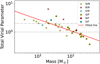 |
Fig. 12 Total virial parameter vs. mass. The legends are the same as those in Fig. 11. |
| In the text | |
|
Fig. 13 Nonthermal velocity dispersion maps of Fields 3, 5, and 26. The green contours show the regions with Mach numbers of greater than 1. The ellipses are the same as those in Fig. 2. |
| In the text | |
|
Fig. 14 Normalized density distribution of 𝓜NT and 𝓜ng in NH3 fragments and MDCs. The contribution of velocity gradient is included in (a) and excluded in (b). |
| In the text | |
|
Fig. 15 Correlation between Tgas and Tdust. The red line shows the linear regression fitting results, and the gray line shows where Tdust = Tgas. |
| In the text | |
|
Fig. A.1 Moment-0 maps with remarkable detection of NH3 (J,K) = (1,1), (2,2), (3,3), (4,4), and (5,5) inversion lines among our observations. The (1,1) maps are plotted from a 3 rms level and in steps of 2σ, while others are plotted from the 2 rms level and in steps of 2σ. The IR-bright, IR-quiet, and starless MDCs are shown as red solid, red dashed, and pink dashed ellipses, respectively. The smaller ellipses present the fragments extracted using the GAUSSCLUMPS algorithm. The blue ones are included in the parameter analysis while the green ones are not. |
| In the text | |
|
Fig. B.1 Distributions of kinetic temperature (left panel), centroid velocity (middle panel), and velocity dispersion (right panel) derived from the simultaneous fitting of NH3 (1,1) and (2,2) inversion lines. The ellipses are the same as those in Fig. A.1. |
| In the text | |
|
Fig. C.1 Compositive images of each field. The background is the Spitɀer three-color images using 8µm (R), 4.5µm (G), and 3.6µm (B) bands. The column density contours and NH3 (1,1) integrated emission contours are over-plotted with green and orange. Cyan and magenta crosses mark the positions of any H2O masers or radio continuum sources, respectively. The ellipses are the same as those in Fig. A.1. |
| In the text | |
|
Fig. D.1 Nonthermal velocity dispersion maps of other fields. The green enclosing areas show the regions with Mach numbers larger than 1. The ellipses are the same as those in Fig. A.1. |
| In the text | |
Current usage metrics show cumulative count of Article Views (full-text article views including HTML views, PDF and ePub downloads, according to the available data) and Abstracts Views on Vision4Press platform.
Data correspond to usage on the plateform after 2015. The current usage metrics is available 48-96 hours after online publication and is updated daily on week days.
Initial download of the metrics may take a while.