| Issue |
A&A
Volume 662, June 2022
|
|
|---|---|---|
| Article Number | A39 | |
| Number of page(s) | 28 | |
| Section | Interstellar and circumstellar matter | |
| DOI | https://doi.org/10.1051/0004-6361/202142601 | |
| Published online | 14 June 2022 | |
Astrochemical modelling of infrared dark clouds
1
Dept. of Space, Earth & Environment, Chalmers University of Technology,
Gothenburg,
Sweden
e-mail: This email address is being protected from spambots. You need JavaScript enabled to view it.
2
Dept. of Astronomy, University of Virginia,
Charlottesville,
VA,
USA
3
Max-Planck-Institut für extraterrestrische Physik,
Gießenbachstrasse 1,
85748
Garching bei München,
Germany
4
School of Physics and Astronomy, University of Leeds,
Leeds
LS2 9JT
UK
5
SOFIA Science Center,
Mountain View,
CA,
USA
6
Max Planck Institute for Astronomy,
Königstuhl 17,
69117
Heidelberg,
Germany
7
Argelander-Institut für Astronomie, Universität Bonn,
Auf dem Hügel 71,
53121
Bonn,
Germany
8
INAF Osservatorio Astronomico di Arcetri,
Largo E. Fermi 5,
50125
Florence,
Italy
9
Centro de Astrobiología (CSIC/INTA),
Ctra. de Torrejón a Ajalvir km 4,
28850
Madrid,
Spain
Received:
6
November
2021
Accepted:
16
March
2022
Abstract
Context. Infrared dark clouds (IRDCs) are cold, dense regions of the interstellar medium (ISM) that are likely to represent the initial conditions for massive star and star cluster formation. It is thus important to study the physical and chemical conditions of IRDCs to provide constraints and inputs for theoretical models of these processes.
Aims. We aim to determine the astrochemical conditions, especially the cosmic ray ionisation rate (CRIR) and chemical age, in different regions of the massive IRDC G28.37+00.07 by comparing observed abundances of multiple molecules and molecular ions with the predictions of astrochemical models.
Methods. We have computed a series of single-zone, time-dependent, astrochemical models with a gas-grain network that systematically explores the parameter space of the density, temperature, CRIR, and visual extinction. We have also investigated the effects of choices of CO ice binding energy and temperatures achieved in the transient heating of grains when struck by cosmic rays. We selected ten positions across the IRDC that are known to have a variety of star formation activity. We utilised mid-infrared extinction maps and sub-millimetre (sub-mm) emission maps to measure the mass surface densities of these regions needed for abundance and volume density estimates. The sub-mm emission maps were also used to measure temperatures. We then used Instituto de Radioas-tromía Milimétrica (IRAM) 30 m observations of various tracers, especially C18O(1-0), H13CO+(1-0), HC18O+(1-0), and N2H+(1-0), to estimate column densities and thus abundances. Finally, we investigated the range of astrochemical conditions that are consistent with the observed abundances.
Results. The typical physical conditions of the IRDC regions are nH ~ 3 × 10⁴ to 105 cm−3 and T ≃ 10 to 15 K. Strong emission of H13CO+(1-0) and N2H+(1-0) is detected towards all the positions and these species are used to define relatively narrow velocity ranges of the IRDC regions, which are used for estimates of CO abundances, via C18O(1-0). We would like to note that CO depletion factors are estimated to be in the range fD ~ 3 to 10. Using estimates of the abundances of CO, HCO+, and N2H+, we find consistency with astrochemical models that have relatively low CRIRs of ζ ~ 10−18 to ~10−17 s−1, with no evidence for systematic variation with the level of star formation activity. Astrochemical ages, which are defined with a reference to an initial condition of all H in H2, all C in CO, and all other species in atomic form, are found to be <1 Myr. We also explore the effects of using other detected species, that is HCN, HNC, HNCO, CH3OH, and H2CO, to constrain the models. These generally lead to implied conditions with higher levels of CRIRs and older chemical ages. Considering the observed fD versus nH relation of the ten positions, which we find to have relatively little scatter, we discuss potential ways in which the astrochemical models can match such a relation as a quasi-equilibrium limit valid at ages of at least a few free-fall times, that is ≳0.3 Myr, including the effect of CO envelope contamination, small variations in temperature history near 15 K, CO-ice binding energy uncertainties, and CR-induced desorption. We find general consistency with the data of ~0.5 Myr-old models that have ζ ~ 2-5 × 10⁻¹⁸ s−1 and CO abundances set by a balance of freeze-out with CR-induced desorption.
Conclusions. We have constrained the astrochemical conditions in ten regions in a massive IRDC, finding evidence for relatively low values of CRIR compared to diffuse ISM levels. We have not seen clear evidence for variation in the CRIR with the level of star formation activity. We favour models that involve relatively low CRIRs (≲10−17 s−1) and relatively old chemical ages (≳0.3 Myr, i.e. ≳3tff). We discuss potential sources of systematic uncertainties in these results and the overall implications for IRDC evolutionary history and astrochemical models.
Key words: astrochemistry / cosmic rays / ISM: clouds / ISM: abundances
© ESO 2022
1 Introduction
Infrared dark clouds (IRDCs) are cold (T < 25 K) (e.g. Pillai et al. 2006; Peretto et al. 2010; Lim et al. 2016) and dense (nH ≳ 103 cm−3) (e.g. Kainulainen & Tan 2013; Lim et al. 2016) regions of the interstellar medium (ISM) that have the potential to host the formation of massive stars and star clusters (for a review, see, e.g. Tan et al. 2014). Thus, it is important to study the physical and chemical properties of IRDCs to understand the initial conditions for the formation of these massive stellar systems.
One important astrochemical process that is expected to occur in the cold, dense conditions of IRDCs is the freeze-out of certain molecules to form ice mantles around dust grains, thus depleting their abundance in the gas phase. The CO depletion factor (fD,CO) is defined as the ratio of the CO gas phase abundance if all C was present as gas phase CO compared to the actual abundance. For example, in the filamentary IRDC G035.39-00.33 (Cloud H), this depletion factor has been measured to be ~3 on parsec scales by Hernandez et al. (2012) and up to ~10 in some positions by Jiménez-Serra et al. (2014).
High CO depletion factors are generally expected in cold conditions, that is when T ≲ 20 K. The rate of CO depletion scales inversely with density, and the timescale to achieve a high depletion factor can be relatively short, that is shorter than the free-fall time for densities nH ≳ 103 cm−3. In this cold temperature regime, the equilibrium abundance of gas phase CO is then expected to be set by a balance between the freeze-out rate and rates of non-thermal desorption processes, that is photodesorption (including by UV photons induced by cosmic rays [CRs]) and by direct CR desorption, that is due to localised transitory heating of dust grains when impacted by a CR (Hasegawa & Herbst 1993). While CO and other species, such as H2O, are expected to be heavily depleted in cold, dense conditions, from studies of low-mass cores it has been inferred that N-bearing species suffer lower amounts of depletion (e.g. Caselli et al. 1999; Crapsi et al. 2007).
In regions where CO is highly depleted and the ortho-to-para ratio of H2 has declined to small values, another astrochemical process that is expected to occur is the build-up of relatively large abundances of H2D+, which in turn can lead to the deuteration of species such as N2H+. Relatively high levels of deuteration of N2H+ have been observed in IRDCs on both parsec scales (Barnes et al. 2016) and in more localised, sub-parsec scale cores (e.g. Kong et al. 2016). These studies have concluded that the conditions in these IRDCs are likely to be relatively chemically evolved, that is with the gas having been in a cold and dense state for at least several local free-fall times in order to achieve the high levels of deuteration that are observed. However, this is not a unique solution: models of relatively rapid collapse of cores can achieve the high observed levels of deuteration if the CR ionisation rate (CRIR) is relatively high. For example, Hsu et al. (2021) have presented models of a massive (60 M⊙ ) core that can achieve abundance ratios of [N2D+] / [N2H+] ~ 0.1 within one free-fall time of ~80 000 yr if the CRIR is ~10−16 s−1.
In addition to the deuteration process, much of interstellar chemistry is driven by CR ionisation, and the CRIR, ζ, (defined as the rate of ionisations per H nucleus) is an important parameter of astrochemical models. Examples of inferred values of CRIR include the study of the H13CO+ emission and  absorption towards seven massive protostellar cores by van der Tak & van Dishoeck (2000), who estimated ζ - (2.61.8) × 10−17 s−1. More recent studies of hot cores with more sophisticated chemical networks include the work of Barger & Garrod (2020), who derived more elevated levels of CRIRs. Studies of the diffuse ISM have found values of ζ ≃ 2 × 10⁻¹⁶ s−1 (e.g. Neufeld & Wolfire 2017). In regions of active star formation, such as OMC-2 FIR 4, much higher values of CRIR, ≳10−15s−1, have been reported (Ceccarelli et al. 2014; Fontani et al. 2017; Favre et al. 2018), which may be explained by local production in protostellar accretion and/or outflow shocks (Padovani et al. 2016; Gaches & Offner 2018). Another region where the CRIR is inferred to be very high is the Galactic Centre, with values of ζ > 10−15 s−1 (Carlson et al. 2016).
Lower energy CRs, which dominate the CRIR, are expected to be absorbed by high column densities of gas and potentially more easily shielded by magnetic fields, whose strength increases in denser regions (Crutcher 2012; however, see Silsbee et al. 2018). Thus, it is possible that the CRIR in IRDCs may be smaller than that of the diffuse ISM in which they reside. To date, there have been relatively few studies of the CRIR in IRDCs.
IRDCs have the advantage of being probed by mid-infrared (MIR) extinction (MIREX) mapping methods (e.g. Butler & Tan 2009, 2012; Kainulainen & Tan 2013), which yield measurements of cloud mass surface density, Σ. Herschel sub-mm emission maps also constrain Σ and additionally provide a measure of the dust temperature, although careful subtraction of contributions from the diffuse Galactic plane are important (Lim et al. 2016). IRDCs are expected to be at a relatively early evolutionary stage, which should simplify their modelling, especially with respect to hot cores (e.g. van der Tak & van Dishoeck 2000; Gieser et al. 2019). However, studies with ALMA and Herschel do indicate that active star formation can be proceeding even in MIR-dark regions of the clouds (e.g. Tan et al. 2016; Kong et al. 2019; Moser et al. 2020).
In this paper, we aim to constrain the astrochemical conditions, including CRIR and chemical age, in ten different positions in the massive IRDC G28.37+00.07. We first present a grids of astrochemical models, based on the work of Walsh et al. (2015), that cover a wide range of physical conditions, including those relevant to IRDCs (Sect. 2). We next, in Sect. 3, measure the physical properties of mass surface density (Σ), number density (nH) and temperature (T) of the IRDC regions, followed by measurements of the column densities and thus abundances of various molecules and molecular ions from IRAM-30 m telescope observations. Then, in Sect. 4, we first discuss the derived abundances, then determine which parts of the multi-dimensional astrochemical model parameter space, including CRIR and time, are consistent with the observations. We also discuss potential effects of systematic uncertainties in the measurements of abundances and astrochemical modelling. We present our conclusions in Sect. 6.
2 Astrochemical model
2.1 Overview of the model
We use the astrochemical model developed by Walsh et al. (2015) to predict the evolution of abundances of different species in the gas and grain ice mantle phases. The model uses a gasphase network extracted from the UMIST 2012 Database for Astrochemistry (McElroy et al. 2013), complemented by both thermal and non-thermal gas-grain processes, including CR-induced thermal desorption (CRID) (with standard value for CR-induced temperature of Tcrid = 70 K), photodesorption, X-ray desorption, and grain-surface reactions. The reaction types included in the astrochemical code are described in Walsh et al. (2010) and the subsequent works (Walsh et al. 2012, 2013, 2014, 2015).
For the first model grid (‘Grid 1’) we have adopted the default CO ice binding energy of 855 K and we have switched off CR-induced thermal desorption reactions (Hasegawa & Herbst 1993), since their rates are highly uncertain (Cuppen et al. 2017). Still, CR-induced photoreactions are included, including those that lead to desorption of species from grain surfaces. Grid 1 is the fiducial model we have used for most of our investigation. However, as we discuss later, after comparison with the observational results we find the need to investigate the following changes in the astrochemical modelling, that is ‘Grid 2’: an increase in the CO ice binding energy to 1100 K, relevant in more realistic situations in which CO is mixed with water ice (Öberg et al. 2005; Cuppen et al. 2017); CRID reactions turned on with various values of Tcrid explored up to about 100 K. In all of our modelling we do not include any X-ray background, so the reactions involving X-rays do not play any role.
Overall the network includes a total of 8763 reactions following the time evolution of the abundances of 669 species. The elements that are followed in the network and their assumed initial abundances are shown in Table 1. All elements are initially in atomic form, except for: H, which is almost entirely in the form of H2; C, which is entirely in the form of CO; and 44% of O that is in the form of CO. This choice is made given that IRDCs are expected to typically be structures within larger-scale molecular clouds.
We have adopted the standard parameter values of a Draine FUV radiation field equal to 6.4 × 10⁻³ erg cm−2 s−1 and a Habing FUV field equal to 4.0 × 108 cm−2 s−1. Other standard parameters are the assumed dust particle radius of a0 = 0.1 μm, so that the grain surface area per H nucleus is 1.63 × 10⁻¹⁹ cm2.
Each astrochemical model in a grid is run for a fixed set of values of number density of H nuclei (nH), gas temperature (T), CRIR (ζ), visual extinction (Av), and FUV radiation field intensity (G0). The range of the parameter space of the grid of the models for this work is presented in Table 2. This parameter space is sampled at a resolution of 3 values per decade for density and CRIR. For temperatures, with a focus on lower values, we run models at 5, 10, 15, 20, 25, 30, 40, 50,…, 100, 120,…, 200, 250, 300,…, 500, 600,…, 1000 K. For Av, we run models at 1, 2, 3, 4, 5, 7, 10, 20, 50, 100 mag. We only run models with one value of external FUV radiation field, that is G0 = 4, which is the value expected in the inner Galaxy relevant to most IRDCs (Wolfire et al. 2010). In any case, the typical values of extinctions in IRDCs are very high, so that the external FUV radiation field is expected to play a negligible role in the chemical evolution.
With the above choices, we have a total of 137 750 different physical models in each grid. Each of these models is evolved in time for 108 yr, with a sampling of 100 outputs per decade in time (after 103 yr). We note that while we have developed here a relatively wide range of models for a first general exploration, when modelling IRDCs, we focus on a much narrower range of conditions that are constrained by observational data on the clouds.
Fiducial initial abundances.
Model grid parameter space.
2.2 CO depletion factor
In this section, we study how the CO depletion factor, fD, varies with astrochemical conditions. CO is typically the second most abundant molecule in molecular clouds after H2 and so it is important to understand its behaviour. One of the main expectations is that CO freezes out rapidly from the gas phase at temperatures ≲20 K, but then with eventual abundances set by a balance of the non-thermal desorption processes from the grains.
In the following, we define fD via:
![Mathematical equation: ${f_{\rm{D}}}\left(t \right) = {{1.4 \times {{10}^{- 4}}} \over {X\left[{{\rm{CO}}} \right]\left(t \right)}},$](/articles/aa/full_html/2022/06/aa42601-21/aa42601-21-eq2.png) (1)
(1)
where 1.4 × 10⁻⁴ is the initial gas phase abundance of CO with respect to H nuclei in our models (i.e. assuming all C is in this form) and X[CO](t) is the actual gas phase abundance of CO with respect to H nuclei, which evolves in time.
To explore the time evolution of fD and its dependence on density, temperature, CRIR and Av, we choose a fiducial reference case with nH = 105 cm−3, T = 15 K, ζ = 10−17 s−1 and Av = 100 mag. We then vary each of these variables systematically, while holding the others constant. The results are shown in Figs. 1a-d). Simple profiles of fD versus these environmental variables at several fixed times are shown in Figs. 2a-d). The time evolution of the abundances of CO, HCO+ and N2H+ are shown in Figs. 3a-d. We now discuss these results in the following four sub-sections.
2.2.1 Dependence on density
In the high density regime, nH ≳ 105 cm−3, the general trend shown in Fig. 1a is that the CO depletion factor increases with time and can reach very high values, fD ≳ 20, within a few Myr. As expected, the evolution proceeds more quickly at higher densities, which lead to higher rates of CO molecules hitting and sticking to the dust grains.
At low densities, nH ≲ 102 cm−3, the freeze-out rates become very low and the desorption rates are high enough to keep most CO in the gas phase. We note that at these densities and at relatively higher CRIRs (>10−16 s−1) (not shown in Fig. 1a) competing processes that destroy CO, that is via interaction with CR-produced He+ or CR-induced FUV photons, become more important (it is important to note that when Av = 100 mag, the destruction of CO via external FUV photons is unimportant). The system can then evolve to having most of the C in atomic or ionised form, and hence the CO abundance is lowered and fD appears large.
Focusing on the density range that is relevant to IRDCs (at least as averaged on ~parsec scales), that is nH ~ 104 to 105 cm−3, we see from Fig. 2a that after 100000 yr fD is still quite small (≲2) at the low density end of this range, but is rising steeply with density at the high-density end. By 1 Myr, it is still relatively low at the low density end, while at the high-density end of the range it is approaching quasi-equilibrium values of fD ≳ 100 for Grid 1 and fD ≳ 10 for Grid 2, which would hold even at ~10 Myr. However, as we see later, this evolution of fD with time and its dependence on density can be very sensitive to the temperature in the range from ~ 15 to 20 K.
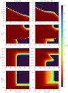 |
Fig. 1 Time evolution of CO depletion factor, fD, evaluated in astrochemical model Grid 1 (left column) and Grid 2 (right column) as a function of the environmental variables of: (a) top row: number density of H nuclei, nH; (b) second row: temperature, T; (c) third row: cosmic ray ionisation rate, ζ; (d) fourth row: visual extinction, Av. In each panel the three remaining variables are held fixed at their fiducial level (i.e. nH = 105 cm−3, T = 15 K, ζ = 10−17 s−1, An = 100 mag). Each time-evolving model is shown by a horizontal line with fD indicated by the colour scale. |
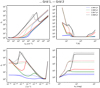 |
Fig. 2 CO depletion factor, fD, evaluated in astrochemical model Grid 1 (dotted lines) and Grid 2 (solid lines), at fixed times of 105 (blue), 106 (green), 107 (red) and 108 yr (black) as a function of the environmental variables of: (a) top left: number density of H nuclei, nH; (b) top right: temperature, T; (c) bottom left: cosmic ray ionisation rate, ζ; (d) bottom right: visual extinction, Av. In each panel, the three remaining variables are held fixed at their fiducial level, that is nH = 105 cm−3, T = 15 K, ζ = 10−17 s−1, Av = 100 mag. |
2.2.2 Dependence on temperature
Time dependant evolutions of fD at different temperatures are shown in Figs. 1b and 2b. The actual gas phase abundances of CO versus time for these models are shown in Fig. 3, along with similar evolutions of HCO+ and N2H+. The strong dependence of fŋ evolution with T in the range from ~10-50 K is clearly illustrated, that is above this temperature range, gas phase CO remains the main reservoir of C. At temperatures ≳500 K, C is still mostly in the gas phase, but mostly in the form of HCN, rather than CO.
2.2.3 Dependence on cosmic ray ionisation rate
Time dependant evolutions of fD at different CRIRs are shown in Figs. 1c and 2c. The actual gas phase abundances of CO versus time for these models are shown in Fig. 3c, along with similar evolutions of HCO+ and N2H+. In this figure, we sometimes see oscillations in the abundances of CO, HCO+ and N2H+, that is in the models with high CRIR and where the condition 1018 cm−3 s < nH/ζ < 2.2 × 1018 cm−3 s. Such behaviour has been noted in the previous study of Maffucci et al. (2018), corresponding to the high ionisation phase (HIP) case discussed by Roueff & Le Bourlot (2020). More generally, the results of Figs. 1c and 2c indicate that as ζ increases, CO depletion begins later in time, but reaches a lower equilibrium value. A different mode of evolution occurs at the highest value of CRIR (ζ = 10−13 s−1), in which C is mostly in the form of C+.
2.2.4 Dependence on visual extinction
Time dependant evolutions of fD at different levels of Av are shown in Figs. 1d and 2d. The actual gas phase abundances of CO versus time for these models are shown in Fig. 3d, along with similar evolutions of HCO+ and N2H+. These figures show that in the models with Av > 5 mag, CO evolution has little dependency on the level of visual extinction so that CO depletion becomes large after about 1 Myr for Grid 1 and after about 10 Myr for Grid 2, no matter the value of Av.
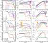 |
Fig. 3 Time evolutions of the abundances of CO (left column), HCO+ (middle column) and N2H+ (right column) evaluated in astrochemical model Grid 1 (dotted lines) and Grid 2 (solid lines), exploring the effects of the environmental variables of: (a) top row: number density of H nuclei, nH; (b) second row: temperature, T; (c) third row: cosmic ray ionisation rate, ζ; (d) bottom row: visual extinction, Av. In each row, the three remaining variables are held fixed at their fiducial level (i.e. nH = 105 cm−3, T = 15 K, ζ = 10−17 s−1, Av = 100 mag). |
3 Observational data and abundance estimates
3.1 Molecular line data
The rotational transitions listed in Table 3 were mapped towards the IRDC G28.37+00.07 (hereafter Cloud C, Butler & Tan 2009, 2012) in August 2008, May 2013 and September 2013 using the IRAM (Instituto de Radioastromía Milimétrica) 30 m telescope in Pico Velata, Spain. Observations were performed in On-The-Fly mode with map size 264" × 252"; central coordinates α = 18h42m52.3s, δ = -4o02'26.2"; and a relative off position of (-370", 30"). An angular separation in the direction perpendicular to the scanning direction of 6" was adopted.
The VESPA receiver was utilised for observations of C18O(1-0) and N2H+(1-0), which provided a spectral resolution of 20 kHz, corresponding to a velocity resolution of 0.053 and 0.063 km s−1, respectively. The other species were observed using the FTS spectrometer with 200 kHz resolution, corresponding to velocity resolutions of ~0.4 to 0.7 km s−1. In the worst case, that is at the lowest frequency of 81.5 GHz, the angular resolution of the molecular line data has a half power beam width (HPBW) of 32" (corresponding to 0.78 pc at the 5 kpc distance of the IRDC). Peak intensities were measured in units of antenna temperature,  , and converted into main-beam temperature, Tmb. Beam and forward efficiencies of 0.73 and 0.95, respectively, for ν ~ 145 GHz, and 0.86 and 0.95 for ν ~ 86 GHz were used. The final data cubes were produced using the CLASS and MAPPING software within the GILDAS package1.
3.2 Mass surface density and temperature data
The mid-infrared (MIR) extinction (MIREX) map of Butler & Tan (2012), derived from 8 μm Spitzer-IRAC imaging data, with the near-infrared (NIR) correction of Kainulainen & Tan (2013), was used as a first method to estimate the mass surface density, Σ, of selected regions in the IRDC. The advantage of this map is that it has a high angular resolution of 2" and the derivation of Σ does not depend on the temperature of the cloud. The disadvantages of the map are that it cannot make a measurement in regions that are MIR bright. Furthermore, the map saturates at values of Σ ~ 0.5 g cm−2, that is in regions with Σ approaching this value the map underestimates the true value of Σ.
An independent measure of Σ for the IRDC has been derived by Lim et al. (2016) based on Herschel-PACS and SPIRE submillimetre (sub-mm) emission imaging data, with this analysis also simultaneously yielding an estimate of the dust temperature. These maps have an angular resolution of 18" for the Σ map and 36" for the T map, that is much lower than that of the MIREX map. As discussed by Lim et al. (2016), there are significant effects due to galactic plane foreground and background emission that contaminate the emission arising from the IRDC itself. In our analysis, we make use of the map derived from the galactic Gaussian (GG) foreground-background subtraction method.
Observed molecular species, rest frequencies, rotational quantum numbers of the transitions, rotational constants, rotational partition function, Einstein A coefficients, energy of lower state, degeneracy of upper state, velocity resolution, Beff and HPBWs.
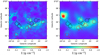 |
Fig. 4 (a): MIREX derived mass surface density map of IRDC G28.37+00.07 from Kainulainen & Tan (2013) (scalebar is in g cm−2). The 10 regions selected for our astrochemical study are marked with circles, labelled 1 to 10. Regions 1 to 6 (red) are known to harbour some star formation activity, while regions 7-10 have been specifically selected to avoid known protostellar sources. (b): sub-mm emission derived mass surface density map of the IRDC from Lim et al. (2016) using the Galactic Gaussian method of foreground-background subtraction (scalebar is in g cm−2). We note that it is of significantly lower angular resolution than the MIREX map (see text). The analysed positions are marked as in (a). |
3.3 Ten selected IRDC regions
From the final data cubes, we extracted molecular line spectra from ten regions in the IRDC (see Fig. 4). Each region has a circular aperture of radius 16", which was set so that the angular resolution of the HPBW of the lowest frequency transition, that is from HC18O+(1-0), fits within the region. At the 5 kpc distance of the IRDC, the radius of each region corresponds to 0.39 pc.
The locations of the 10 positions were selected for having relatively high values of Σ and for having a range of star formation activities. In particular, positions P1 to P6 (shown with red circles in Fig. 4) are known to be sites of active star formation based on the presence of CO outflows (Kong et al. 2019) and containing Herschel-Hi-GAL 70 μm point sources (Moser et al. 2020). However, these positions are still dark structures at 8 μm: indeed the P1 to P6 positions correspond approximately to the MIREX Σ peaks of C1, C2, C4, C5, C6 and C8, respectively, identified and characterised by Butler & Tan (2012).
The positions from P7 to P10 (shown with black circles in Figs. 4 and 5) are not directly associated with massive condensations previously identified within the cloud (Rathborne et al. 2006; Butler & Tan 2009, 2012) and have been selected for being relatively quiescent in terms of their star formation activity (Kong et al. 2019; Moser et al. 2020).
From the two mass surface density maps shown in Fig. 4, we have measured the average values of ∑MIREX and ∑sub-mm in each of the ten regions P1 to P10 (see Table 4). This also allows an estimate of Nh, assuming a mass per H of μH = 1.4mH = 2.34 × 10⁻²⁴ g (i.e. approximately due to nHe - 0.1nH and ignoring contributions from other species). We assume an uncertainty of ~30% in the measurements of Σ and Nh (Kainulainen & Tan 2013; Lim et al. 2016).
We have then estimated the average total amount of visual extinction, Av, through each region using the standard dust model assumptions of Kainulainen & Tan (2013), that is:
 (2)
(2)
However, we then divide this estimate of the total extinction through the region by a factor of 4 in order to obtain an estimate of the typical extinction from the nearest boundary of the IRDC, that is Āv = Av,tot/4
We have estimated the average number density of H nuclei, nH, in each region by assuming the material is distributed in a spherical volume with radius equal to the circular aperture radius of the region projected on the sky. These values are also listed in Table 4.
Finally, by using the dust temperature map from Lim et al. (2016), we have estimated the Σ-averaged T values for the ten selected positions (Fig. 5). These values are also listed in Table 4. The uncertainties in T are assumed to be at the level of 30% (Lim et al. 2016).
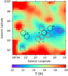 |
Fig. 5 Sub-mm emission derived dust temperature map of IRDC G28.37+00.07 from Lim et al. (2016) using the galactic Gaussian method of foreground-background subtraction (scalebar in K). The ten regions selected for our astrochemical study are marked with circles, labelled 1 to 10, as in Fig. 4. |
3.4 Molecular abundances
We now estimate column densities of the nine observed species listed in Table 3 in the 10 regions of the IRDC and use these results to calculate their abundances with respect to the total H nuclei, that is Nx/Nh. For the column density estimation we have used Eq. (A4) of Caselli et al. (2002):
![Mathematical equation: $\matrix{{{N_{\rm{X}}}} \hfill & {= {{8\pi {v^2}} \over {A{g_u}{c^3}}}{k \over h}{1 \over {{J_v}\left({{T_{{\rm{ex}}}}} \right) - {J_v}\left({{T_{{\rm{bg}}}}} \right)}}} \hfill \cr {} \hfill & {\times {{{Q_{{\rm{rot}}}}} \over {1 - \exp \left({{{- hv} \mathord{\left/ {\vphantom {{- hv} {\left[{k{T_{{\rm{ex}}}}} \right]}}} \right. \kern-\nulldelimiterspace} {\left[{k{T_{{\rm{ex}}}}} \right]}}} \right)}}{1 \over {\exp \left({{{- {E_L}} \mathord{\left/ {\vphantom {{- {E_L}} {\left[{k{T_{{\rm{ex}}}}} \right]}}} \right. \kern-\nulldelimiterspace} {\left[{k{T_{{\rm{ex}}}}} \right]}}} \right)}}\int {{T_{{\rm{mb}}}}} {\rm{d}}v,} \hfill \cr} $](/articles/aa/full_html/2022/06/aa42601-21/aa42601-21-eq5.png) (3)
(3)
where v is the frequency of the observed transition, A is the Einstein coefficient obtained from the CDMS catalog2, gu = 2J + 1 is the statistical weight of the upper level, El is the energy of the lower level, and Jv(Tex) and Jv(Tbg) are the equivalent RayleighJeans (RJ) excitation and background temperatures, respectively. For these we set Tex = 7.5 K based on the multi-transition CO study of an IRDC by Hernandez et al. (2012), while Tbg = 2.73 K from the cosmic microwave background (CMB). Finally, Qrot is the rotational partition function at the assumed Tex. For each molecule, Qrot has been calculated by fitting its values from jet propulsion laboratory (JPL) catalogue3, except in the case of N2H+ and HCN for which, since their main rotational transitions split into hyperfine components, the partition function reported in the JPL catalogue includes an additional factor and it does not coincide with the pure rotational partition function. Hence, for N2H+ and HCN, we have calculated Qrot as:
 (4)
(4)
where, Ej - J(J + 1)hB is the energy of the J level and B is the rotational constant of the molecule. The various parameters used to derive the abundances of the species are listed in Table 3. Finally, we note that  and Nhcn obtained from Eq. (3) have been corrected for the transition statistical weights of 0.11 and 0.3333, respectively, since only one of the hyperfine lines was used in each case to derive total abundances.
In deriving column densities from the observed spectra, which are shown in Figs. 6 and 7, we must make a choice of the velocity range over which to integrate the line intensities. From inspection of the spectra, this range is chosen to have a common extent of 77 to 82 km s−1, motivated by the goal of covering the dense gas tracers of H13CO+(1-0), HC18O+(1-0) and N2H+ (1-0). Examining the spectra of Figs. 6 and 7, we see that C18 O(1-0) generally shows emission from several components that span a broader velocity range than the above dense gas tracers. In our analysis, we only measure the CO column density from the part of C18O(1-0) emission that falls in the velocity range from 77 to 82 km s−1.
To estimate the uncertainties in the total column densities, we consider the following factors. First is the uncertainty in the integrated intensity of each line, which we assess to be equal to the noise integrated in a line-free spectral range and calculated as:
 (5)
(5)
where n is the number of channels, each of velocity width dv, that are summed in the integration and ΔTmb,noise is the noise in an individual channel.
Second is the systematic uncertainty due to the need to assume a value of Tex. We note that Tex = 7.5 K has been adopted for all the species. If Tex is varied by ±30% about this value, the estimated total column density changes by ~7-28%. For most species, this systematic error dominates over that due to the noise in the integrated intensity. In our analysis, we estimate the overall uncertainty in total column densities by summing the above two sources of uncertainties in quadrature. However, we note that there are other potential sources of systematic error, such as the assumption that the emission in the particular chosen velocity range is a good representation of the physical component of the molecular cloud that is being modelled.
For some of the species, like CO, HCO+ and HNC, the column density is estimated by conversion from a rarer isotopologue. This involves another source of systematic uncertainty. For these conversions, we assume [12C]/[13C] = 40.2 ± 8.0 (Zeng et al. 2017) and [16O]/[18O] = 318 ± 64 (Hezareh et al. 2008) and these levels of uncertainty are also propagated in quadrature for the final column density estimate.
We note that, since no significant signal is detected for the HC18O+(1-0) transition towards the positions P6, P7, P8, P9, and P10, we have estimated their HC18O+ column density from the average of their spectra. Then, we have apportioned this column density among the five positions in proportion to their H column densities.
The final step of the analysis is to estimate abundances of species with respect to H nuclei that are assumed to be present in the same molecular cloud component. For this we simply divide the above estimates of total species column density by the estimate of H nucleus column density obtained previously either via Herschel-observed sub-mm dust emission or via MIR extinction. Each of these methods is assumed to have a 30% uncertainty, which is summed in quadrature for the final abundance estimate. The obtained results are summarised in Table 4. We note that the H column densities obtained by both methods are themselves quite similar (see above) and, for simplicity, in the remaining analysis we adopt those estimates based on the sub-mm dust continuum emission.
Estimated physical properties and molecular abundances of the P1 to P10 positions in IRDC G28.37+00.07.
4 Results
4.1 Abundances, including density dependence
Here, we summarise the abundances of the various species obtained in the IRDC positions (see also Table 4). For CO, we find a typical value of [CO] ≡ Nco/Nh ~ 2 × 10⁻⁵, which corresponds to a CO depletion factor of fD ~ 7. In Fig. 8a we plot fD versus nH, which reveals a trend of increasing depletion factor (i.e. smaller gas phase CO abundance) with increasing density. While correlated uncertainties are present in the measurements of fD and nH (estimated via Nh), the trend is significant, given a Pearson correlation coefficient of r = 0.93. For completeness, the same information about the trend of [CO] with nH is also shown in Fig. 9a, with this figure showing the abundances versus density for all eight species measured in our study.
Theoretically, for a given set of conditions, including cloud age, one expects higher CO depletion factors at higher densities, that is due to higher rates of freeze-out leading to shorter freeze-out timescales. To illustrate this quantitatively, Fig. 8a shows some example models of the time evolution of fD versus nH, with other parameters set to values of T = 15 K, Av = 20 mag, and three values of ζ = 10−18, 10−17 and 10−16 s−1 explored. The observed trend of fD versus nH can be explained by a model in which the ten positions have fairly similar ages of 2 × 10⁵ yr. We note that this result is quite insensitive to certain choices of the astrochemical models, such as ζ, Av (for values >5 mag) and T (for values <20 K). However, as we discuss below, certain choices in the models about how nonthermal desorption processes are implemented can have impact on the inferred chemical age from these data.
Figure 8b plots fD versus Āv. While we see a trend of increasing observed fD versus Āv , we note that Āv ∝ Nh ∝ nH. At a given age and volume density, the astrochemical models do not predict a significant variation of fD with Av (at least for Av > 5 mag, which is the relevant range). Thus, we consider that trend we observe here is more likely to be caused by variations in density in the regions.
For HCO+, using emission from H13CO+ we infer typical abundances of [HCO+] ~ 4× 10⁻¹⁰. The abundances inferred from HC18O+ are systematically larger by about 30%. However, such a difference is within the isotopologue ratio uncertainties. While the two lowest density regions, P6 and P10, are seen to have the highest abundances, -6 × 10⁻¹⁰, the overall correlation with density is not as strong as in the case of [CO] (see Fig. 9b).
We estimate [N2H+] ~10−10 on average (see Fig. 9c). Again, the lowest density region has the highest abundance, but, as with HCO+, there is no significant trend with density. Similar results are seen for HNC, with typical abundance of 6 × 10⁻¹⁰ (Fig. 9d) and HCN, with typical abundance of [HCN] ~ 10−10 (Fig. 9e).
Finally, we find [HNCO] ~ 3 × 10⁻¹⁰, [H2CO] ~ 5 × 10⁻¹⁰ and [CH3OH] ~ 10−9 as typical values (see Figs. 9f, g and h). Here there are hints of a bifurcation in the regions, with P1, P6, P7 and P8 having relatively low values, and the other six regions having abundances that are several times larger.
We note that P7 and P8 were specifically chosen to be in regions that are relatively quiescent with respect to star formation activity as traced by CO(2-1) outflows (Kong et al. 2019), while still containing relatively dense structures. P1 also includes the candidate C1-N and S massive pre-stellar cores (Tan et al. 2013), that is significant quantities of dense, quiescent gas, although there are also two protostellar sources (C1-Sa and C1-Sb) in the same region. P6 also appears to be quiescent, that is not containing a 70 μm detected protostar (Moser et al. 2020), but is outside the region mapped for CO(2-1) outflows. Thus, we tentatively conclude that regions with relatively low star formation activity also have relatively low abundances of the relatively complex species of HNCO, H2CO and CH3OH. Such a result could be due to requirement of protostellar warming or outflow shock activity to liberate these species efficiently from dust grain ice mantles.
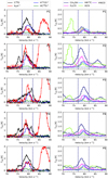 |
Fig. 6 Fig. 6. – Spectra of observed species at positions P1-P5. The dashed lines indicate the velocity range 77-82 km s−1, which has been selected to cover the dense gas as traced by N2H+ and H13CO+. In the left column panels, the amplitudes of the signals of H13CO+(1-0), HC18O+ (1-0) and N2H+(1-0) have been multiplied by a factor of three for clarity of display. |
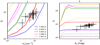 |
Fig. 8 (a): CO depletion factor (fd) versus number density of hydrogen nuclei (nH). The data for each position are shown, along with their uncertainties. Astrochemical models are shown for ages ranging from 105 yr to 107 yr and for ζ = 10−18 s−1 (dotted lines) and 10−17 s−1 (solid lines) and 10−16 s−1 (dashed lines) with other parameters set to be T = 15 K and Av = 20 mag. (b): CO depletion factor (fd) versus visual extinction (Av). The data for each position are shown, along with their uncertainties. Astrochemical models are shown here for nH = 105 cm−3, T = 15 K and ζ = 10−17 s−1 with solid lines (colors represent different times, as in legend of (a)). An equivalent model for nH = 104 cm−3 is shown with dotted lines. |
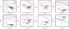 |
Fig. 9 Observed abundances of (a) CO, (b) HCO+, (c) N2H+, (d) HNC, (e) HCN, (f) HNCO, (g) H2CO and (h) CH3OH versus n∏. Astrochemical model results are also shown for ζ = 10−18 s−1 (dotted lines), 10−17 s−1 (solid lines) and 10−16 s−1 (dashed lines) with other parameters set to be T = 15 K and Av = 20 mag. |
Extracted astrochemical parameters of the best models in R, UR and XR regions, using observed abundances of [CO],[HCO+] and [N2H+] as Case 1, and all observed abundances as Case 2.
4.2 Astrochemical implications for cosmic ray ionisation rate and cloud age
In this section we use the abundance measurements of the IRDC positions to constrain conditions in the clouds, especially ζ and t, via the astrochemical models described in Sect. 2. In general, we compare a set of the observed abundances, [Xi]obs in a given position with those of theoretical model abundances, [Xi]theory. We search the model grid parameter space (nH, T, Av,ζ, t) to minimise a χ2 metric of the following form
![Mathematical equation: ${\chi ^2} = \sum\limits_i {{W_i}} {\left[{{{\left({{{\log}_{10}}{{\left[{{X_i}} \right]}_{{\rm{obs}}}} - {{\log}_{10}}{{\left[{{X_i}} \right]}_{{\rm{theory}}}}} \right)} \mathord{\left/ {\vphantom {{\left({{{\log}_{10}}{{\left[{{X_i}} \right]}_{{\rm{obs}}}} - {{\log}_{10}}{{\left[{{X_i}} \right]}_{{\rm{theory}}}}} \right)} {{{\log}_{10}}}}} \right. \kern-\nulldelimiterspace} {{{\log}_{10}}}}\left({{\sigma _i}} \right)} \right]^2}$](/articles/aa/full_html/2022/06/aa42601-21/aa42601-21-eq9.png) (6)
(6)
where σi is an estimate of the uncertainty in the abundance, including the basic observational uncertainty and any allowed theoretical model uncertainty, and Wi; is a weighting factor, which allows certain species to be given greater or lesser importance in the analysis.
4.2.1 Constraints using [CO], [HCO+] and [N2H+] (Case 1)
As first step (Case 1), we only consider the abundances of CO, HCO+ (obtained from H13CO+) and N2H+, that is CO and the two molecular ions in our set of species. We have first searched the entire model grid parameter space to find best fitting models and map out theχ2 landscape. However, unrealistic solutions can be found with low values of χ2, that is at high temperatures (>500 K), where low values of [CO] are caused by gas-phase chemical processing of the CO, rather than by CO freeze out onto dust. Thus, we focus on a restricted (R) search over the ranges: пн = 104-106 cm−3; T = 10-50K and Av = 5-100mag. We also consider ultra-restricted (UR) searches in which nH and Av are set to the closest values in the model grid to those of the observed region and with only adjacent values also considered. For this UR case we limit the search to T = 10-20 K. Finally, we have an extreme-restricted (XR) case where we only search the ζ-t parameter space in the best physically matched model for nH, Av and T (we note that in this case we always set T = 15 K: this is always the closest match, except for P1, where T = 11.8 K, but even here, for simplicity, we consider 15 K for the XR case).
The χ2 landscape in the ζ versus t plane for the XR search at the P2 position (i.e. with nH = 1.0 × 105 cm−3, Av = 20 mag and T = 15 K) with Case 1 ([CO], [HCO+] and [N2H+]) fitting is shown in the central panel of Fig. 10. The surrounding eight panels show the effect on the χ2 landscape of stepping in the model grid to the next higher and lower values of density and temperature, while keeping Av held fixed at 20 mag.
We notice several main features in Fig. 10. First, the best result in the central panel that is matched to the physical conditions of P2 has ζ = 2.2 × 10⁻¹⁸ s−1 and t = 2 × 10⁵ yr and yields a value of χ2 = 0.69. These values are listed in Table 5, along with those obtained for the UR and R searches.
Second, we see that this position of lowest χ2 sits in an ‘island’ that extends to higher values of ζ at earlier times and lower values of ζ at later times. There is also a separate, secondary island of relatively low values of χ2 at later times and higher ζ, with local minimum at t = 2.82 × 10⁶ yr and ζ = 2.2 × 10⁻¹⁶ s−1.
As we vary the density of the model, the above features are broadly preserved, with a shift in the best position to earlier times and higher ζ if the density is raised, and later times and lower ζ if it is lowered. We have also inspected the equivalent figures for the cases with Av = 10 and 50 mag and find only modest differences compared to the An = 20 mag cases. Considering temperature variation, the models at T = 10 K have a similar structure, with the best position now at moderately higher values of ζ, but with worse values of χ2. However, at T = 20 K the results are quite different, with the previous best χ2 island now erased and the new best solutions being at much later times, with the best value unrealistically old.
To understand the above behaviour, we next consider the detailed time evolution of some example models from the XR conditions: we examine the overall best model and the best model in the secondary, late-time island (see Fig. 11). With a temperature of 15 K, for both models the evolution of gasphase CO abundance is initially one of monotonic decline due to freeze-out onto dust grains. At the XR density of nH = 1.0 × 105 cm−3, this reaches the observed depletion factor of ~10 by about 2 × 10⁵ yr, independent of ζ. The influence of the CRIR is seen on the (quasi-)equilibrium level of gas phase CO abundance that is reached, after about 1 Myr. However, even in the case with ζ = 2.2 × 10⁻¹⁶ s−1, this abundance of CO is about 10 times smaller than the observed level. Thus the process of CO freeze-out essentially sets the timescale of the best model.
Next, considering the abundance of HCO+, it is seen to have a fairly constant evolution in time. In the overall best model it is gradually declining in the first few hundred thousand years. Finally, the evolution of [N2H+] shows an early-time rapid rise from very low values associated with our assumed initial conditions, that is all N in atomic form. The rate of this rise is more rapid when ζ is higher. This is followed by a plateau phase and subsequent decline in abundance. The overall best model is achieved on the first time rise of [N2H+], while the higher CRIR later-time model is achieved on the decline from the plateau phase. It is [HCO+] and [N2H+] that mostly set the CRIR of the best model, in particular favouring a low value of ζ = 2.2 × 10⁻¹⁸ s−1. This is illustrated in Fig. 12, where models with ten times higher and lower values of CRIR compared to this value are shown.
Next we consider the results of the UR and R search results for P2. As mentioned, the best fitting models for these search ranges are also listed in Table 5. Figure 13 shows the projected χ2 landscapes in the ζ versus t plane for XR, UR and R searches. We see that the regions of low values of χ2 expand, as expected. The early-time, low-ζ island expands to cover a broader range of times, with the later time solutions being those of lower density and vice versa. In particular, the overall best models are now moved to these later time, lower density, lower ζ regions. However, it should be noted that there are quite widespread regions of relatively low χ2, so the relevance of the particular overall best model is less significant.
Next we consider the Case 1 results for the rest of the IRDC positions. In particular, we next consider the P6 position (Fig. 14), which has been selected to be starless. We see that the overall feature of the χ2 distributions for P6 are quite similar to those of P2. The equivalent figures for the other regions follow the same general patterns and we do not present them here. In general, all these regions also exhibit quite similar χ2 landscapes for their XR, UR and R Case 1 search results.
Thus, in summary, the main features of the Case 1 fitting are that the best solutions have relatively low CRIRs (~10−18s−1) and yield ages in the range ~105 to ~106 yr. There is an extended ‘valley’ of low χ2 values extending to higher CRIR solutions (e.g. ~10−17 s−1), but requiring smaller ages (e.g. 105 yr). This type of solution is based on the gas being in a phase of early CO freeze-out, that is with the age set by the time needed to freeze-out from the adopted initial conditions of all CO in gas phase.
However, as we discuss later in Sect. 5, we consider that there are caveats with this interpretation. In particular, it seems to be unlikely that all the ten selected positions would be in this initial phase of CO freeze out and the implied values of CRIR are relatively low compared to previous estimates in the more diffuse ISM. Thus, we also discuss possible ways in which later-time solutions (t ≳ 1 Myr) can be achieved.
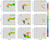 |
Fig. 10 The central panel shows the χ2 landscape (up to values of 30) in the ζ versus t plane for the P2 position for the XR search (i.e. with nH = 1.0 × 105 cm−3, Av = 20 mag and T = 15 K) Case 1 (fitting to abundances of CO, HCO+ and N2H+). The location of the minimum χ2 is marked with a white cross. The surrounding eight panels show the effect on the χ2 landscape of stepping in the model grid to the next higher and lower values of density and temperature (as labelled). Note, Av is held fixed at 20 mag in all these panels (so these are just a subset of the UR search). |
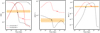 |
Fig. 11 Time evolution of [CO] (gas [dotted] and ice [solid] phases) (left), [HCO+] (middle) and [N2H+] (right) for the overall best fitting model (black lines, ζ = 2.2 × 10⁻¹⁸ s−1) and best ‘late-time’ model (red lines, ζ = 2.2 × 10⁻¹⁶ s−1) for the XR search of the P2 clump, i.e. with nH = 1.0 × 105 cm−3, Av = 20 mag and T = 15 K. The time of the best models along each of these tracks is marked with a ‘+’ symbol. Horizontal dotted lines show the observed values of abundances, with the uncertainties shown by the shaded bands. |
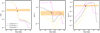 |
Fig. 12 As Fig. 11, but now showing the effect of varying the CRIR by a factor of 10 to higher (magenta) and lower (yellow) values compared to the XR best model value of ζ = 2.2 × 10⁻¹⁸ s−1. The best timescales for each of the models are shown with corresponding ‘+’ symbols, given the observed abundances of the P2 location. |
4.2.2 Constraints using all species (Case 2)
We next show the equivalent results for constraining the astrochemical conditions when the abundances of all the eight species observed at the P2 position are used, which we refer to as Case 2. However, for these additional five species we set their weights to only contribute 25% of the total weighting of χ2, that is 5% each. This choice is made given that we consider that these species have somewhat more uncertain astrochemistry and that, being neutral species, they have a less direct connection to the CRIR than HCO+ and N2H+.
The Case 2 χ2 landscape in the ζ versus t plane for the XR search at the P2 position (i.e. with nH = 1.0 × 105 cm−3, Av = 20 mag and T = 15 K) is shown in the central panel of Fig. 15. The surrounding eight panels show the effect on the χ2 landscape of stepping in the model grid to the next higher and lower values of density and temperature, while keeping Av fixed at 20 mag.
We notice several main features in Fig. 15. First, the best result in the central panel that is matched to the physical conditions of P2 has ζ = 2.2 × 10⁻¹⁷ s−1 and t = 4.47 × 10⁶ yr and yields a value of χ2 = 60.82. These values are listed in Table 5, along with those obtained for the UR and R searches. We see that this position of lowest χ2 sits close to the later-time, higher CRIR region that was found as a secondary solution area in the Case 1 XR search. The previous best χ2 region from Case 1 that is at earlier times and lower CRIRs is still seen in Case 2 as a local minimum of χ2, but now does not contain the global minimum. We note also that for Case 2 the overall values of χ2 are much greater than for Case 1. We examine below the reason for the poorer level of fitting.
As we vary the density of the model, the general, overall shape of the χ2 landscape does not change too much, however, we note that going to higher densities leads to the best fit model being at earlier times (~105 yr) and with relatively high CRIR (ζ = 2.2 × 10⁻¹⁶ s−1). This solution region is also found when the temperature is lowered to 10 K. When raising the temperature to 20 K we see that later time solutions are preferred, with there being some overlap of these with the best region found in the XR case. Similar to Case 1, having inspected the equivalent results for Av = 10 and 50 mag, we find only modest differences compared to the Av = 20 mag cases.
To understand the above behaviour, we next consider the detailed time evolution of some example models from the XR conditions. First, we examine the overall best model (see Fig. 16). As seen before in Case 1, with a temperature of 15 K, the evolution of gas-phase CO abundance is initially one of monotonic decline due to freeze-out onto dust grains. At the XR density of nH = 1.0 × 105 cm−3, this reaches the observed depletion factor of ~10 by about 2 × 10⁵ yr. However, because of the abundance of other species, especially CH3OH, later time solutions are preferred, even though the gas-phase abundance of CO is now in worse agreement compared to the observed value. We also see why the overall value of χ2 is worse, since the abundances of several of the species, such as CO, HNC, HCN, H2CO and CH3OH, are not very well fit even for the best model, with differences greater than a factor of 10.
A comparison of models with different CRIRs is shown in Fig. 17, where models with ten times higher and lower values of ζ compared to that of the best XR model are shown. In general higher values of ζ lead to higher abundances of the considered species and vice versa.
Next, we consider the Case 2 UR and R search results for P2. As mentioned, the best fitting models for these search ranges are also listed in Table 5. Figure 18 shows the projected χ2 landscapes in the ζ versus t plane for XR, UR and R searches. We see that the regions of low values of χ2 expand, as expected. In the UR search, a solution at earlier time and higher CRIR is preferred, which is in a region already seen in Fig. 15. In the less constrained R search, a solution with an unrealistically old age (≫107 yr) is found, although earlier times with only moderately worse χ2 values are apparent. In general, the estimated values of ζ via Case 2 at P2 are higher than those found in Case 1. Later time solutions are also more favoured. However, the overall fits are worse, with larger values of χ2.
Next, we consider the Case 2 results for the rest of the IRDC positions. In particular, we next consider the P6 position (Fig. 19). There are some noticeable differences in the Case 2 χ2 landscapes of P6 compared to P2, especially for the XR and UR searches. For XR in P6 there is a greater preference for earlier time solutions, while for UR a later time solution is favoured. The equivalent figures for the other regions are quite similar and we do not present them here.
Thus, in summary, the main features of the Case 2 fitting are that, compared to Case 1, the best solutions have relatively larger values of CRIRs (~10−17 s−1) and a more extended range of ages, from ~105 to ~107 yr. However, the overall goodness of the fits is worse.
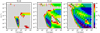 |
Fig. 13 Projected best χ2 values in the ζ versus t plane for the P2 position for the XR (left), UR (middle) and R (right) search methods with Case 1 (fitting to abundances of CO, HCO+ and N2H+). The location of the minimum χ2 is marked with a white cross in each panel. |
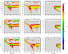 |
Fig. 15 The central panel shows the χ2 landscape (up to values of 100) in the ζ versus t plane for the P2 position for the XR search (i.e. with nH = 1.0 × 105 cm−3, Av = 20 mag and T = 15 K) Case 2 (fitting to abundances of all species). The location of the minimum χ2 is marked with a black cross. The surrounding eight panels show the effect on the χ2 landscape of stepping in the model grid to the next higher and lower values of density and temperature (as labelled). We note that Av is held fixed at 20 mag in all these panels (so these are just a subset of the UR search). |
5 Discussion and extended analysis
Here we investigate the effects of several aspects of the observational analysis and astrochemical modelling that may have a major influence on the fiducial Case 1 results of a preference for relatively early time (~105 yr) and low ζ (~10−18 s−1) solutions. We consider that such young ages are questionable because it is unlikely that all ten regions, P1 to P10, are in such early evolutionary stages with ages similar to their current local free-fall times, tff = (3π∕[32Gρ])1/2 ~ 105 yr (see Table 4). Furthermore, the derived values of CRIR are significantly lower than those derived from previous studies (see Sect. 1).
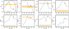 |
Fig. 16 Time evolution of [CO] (gas [dotted] and ice [solid] phases) (top left). The remaining panels show the equivalent panels for the gas phase abundances of the rest of the species for the overall best fitting model (ζ = 2.2 × 10⁻¹⁷ s−1), for the XR search of the P2 clump, that is with nH = 1.0 × 105 cm−3, Av = 20 mag and T = 15 K. The time of the best overall model along each of these tracks is marked with a ‘+’ symbol. Horizontal dotted lines show the observed values of abundances, with the uncertainties shown by the shaded bands. |
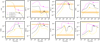 |
Fig. 17 As Fig. 16, but now showing the effect of varying the CRIR by a factor of 10 to higher (magenta) and lower (yellow) values compared to the XR best model value of ζ = 2.2 × 10⁻¹⁷ s−1. The overall best timescales for each of the models are shown with corresponding ‘+’ symbols, given the observed abundances of the P2 location. |
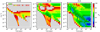 |
Fig. 18 Projected best χ2 values in the ζ versus t plane for the P2 position for the XR (left), UR (middle) and R (right) search methods with Case 2 (fitting to abundances of all species). The location of the minimum χ2 is marked with a black or white cross in each panel. |
5.1 Contamination by envelope CO emission
The CO(1-0) has a much lower critical density than HCO+(1-0) and N2H+ (1-0). While we have made efforts to restrict the velocity range used to estimate the CO column density to closely match that of the higher density tracers, it remains possible that our measurement suffers from contamination from lower density, envelope gas that is surrounding the region of interest, but overlapping in velocity space. To account for this possibility and to investigate its potential effects, we simply assume a contamination level of 90%, and reduce the observed CO column density by a factor of 10 (and we set the uncertainty in CO abundance to then be a factor of 3).
Figure 20 presents XR, UR and R χ2 projections in the ζ versus t plane for P2 with this reduced gas phase CO abundance. We find that later-time solutions are now favoured. For example, the best XR solution has t ≃ 2 × 10⁷ yr and ζ ≃ 2 × 10⁻¹⁸ s−1. However, there is also a degeneracy with higher CRIR and earlier times that yield similarly low χ2 values. Figure 21 shows time histories of abundances for several example XR models that illustrate these kinds of solutions. The observed HCO+ abundance is seen to give a constraint on the CRIR, while that of N2H+ helps select models at relatively later times.
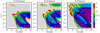 |
Fig. 20 Investigation of effect of CO envelope contamination showing the projected best χ2 values in the ζ versus t plane for the P2 position for the XR (left), UR (middle) and R (right) search methods with Case 1 (fitting to abundances of CO, HCO+ and N2H+). For this fitting, the observed abundance of CO has been reduced by a factor of 10 and the associated uncertainty is set to be a factor of 3. The location of the minimum χ2 is marked with a white cross in each panel. |
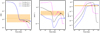 |
Fig. 21 Investigation of effect of CO envelope contamination showing time evolution of [CO] (left), [HCO+] (middle) and [N2H+] (right) for the overall best fitting model (black line, ζ = 2.2 × 10⁻¹⁸ s−1). Here the observed CO abundance has been reduced by a factor of 10 and the total uncertainty set to be a factor of 3. The effects of varying the CRIR by a factor of 10 to higher (magenta) and lower (blue) values compared to the XR best model value are shown. The best timescales for each of the models are marked with corresponding ‘+’ symbols. |
5.2 Influence of temperature near the CO sublimation limit
The next aspect we investigate is that of the precise choice of temperature in the range 15 K to 20 K4. Within this range there is a dramatic difference in the evolution of gas phase CO abundance due to freeze-out on dust grains. Recall also that the early-time solutions found in Case 1 are driven largely by the evolution of CO freeze-out from an initial condition of [CO] ~ 10−4 to observed values of ~10−5 (i.e. CO depletion factor of fD ~ 10).
Figure 22 shows the time evolution of the abundances of CO, HCO+ and N2H+ in the fiducial Case 1 modelling of P2 with finer temperature variation from 15 to 20 K. We see that a small difference in adopted temperature, that is 16 K compared to 15 K, makes a large difference in the gas phase CO abundance during timescales up to ~107 yr. In particular, the model with T = 16 K reaches a quasi-equilibrium gas phase CO abundance of ~ 10−5 after about 300 000 yr, which then persists at about this level for several Myr. Given the sensitivity of this aspect of the astrochemical model to the choice of T and recognising the systematic uncertainties in both the CO ice binding energy and the measurement of T in the IRDC, it is conceivable that the IRDC clumps are in this quasi-equilibrium phase.
In Fig. 23, we show examples of the time evolution of [CO], [HCO+] and [N2H+] at T = 16 K for various CRIRs. Later time solutions are possible, although the preferred value of ζ remains relatively low, ~10−18s−1, set by [HCO+]. The full projected Case 1 χ2 landscapes for P2 with XR, UR and R, but with the temperature always fixed to be T = 16 K, are shown in Fig. 24. Here we see the full extent of these later-time, lower-CRIR solutions.
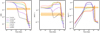 |
Fig. 22 Time evolution of [CO], [HCO+] and [N2H+] for XR conditions for P2, that is nH = 1 × 105 cm−3, Av =20 mag, but with various temperatures from 15 to 20 K. Here, ζ = 1.0 × 10⁻¹⁷ s−1. The horizontal band shows the observed abundances, together with corresponding uncertainties, at P2. |
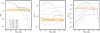 |
Fig. 23 Time evolution of CO, HCO+ and N2H+ abundances in the models with nH = 1 × 105 cm−3, T = 16 K, Av = 100 mag and for different values of ζ. The horizontal band shows the observed abundances together with corresponding uncertainties at P2. |
5.3 Influence of cosmic ray induced desorption (CRID)
When cosmic rays impact dust grains they cause local heating of the material, which can lead to enhanced thermal desorption of species from the ice mantles. This process has been described by Walsh et al. (2010) and incorporated into the astrochemical network. However, so far, in the fiducial modelling described above, we have not included this process due to its inherent large uncertainties. Here we investigate its effects with the standard rates described by Walsh et al. (2010) and Sipilä et al. (2021). In particular, the maximum temperature of the transiently heated grains is assumed to be Tcrid = 70 K (see Sect. 2).
Figure 25 shows the results of modelling of [CO], [HCO+] and [N2H+] for XR conditions for P2 with several different values of ζ. For each ζ we show a model with and without CRID, with the latter being the fiducial models already presented. We see that for [CO] the effect of CRID is, as expected, to maintain a higher gas phase abundance, especially from about 0.5 to 10 Myr. As a result of this higher CO abundance, the level of [HCO+] is also increased in the CRID models.
Figure 26 shows the projected χ2 landscapes in the ζ versus t plane for the Case 1 XR, UR and R search methods for the P2 abundances using models in which CRID is included. While the best overall XR model is similar to that found before without CRID, in general we see that inclusion of CRID raises up the values of χ2 at later times, that is around t = 1 Myr.
We conclude that CRID, along with the already investigated effects of CO envelope contamination and intermediate temperatures in the range 15 to 20 K, can make later time and higher CRIR solutions more consistent with the observational constraints of the P2 position (and other IRDC positions). In the next subsection we use the Case 1 data from all the positions, including the observed trends with density, to give some constraints on combinations of these effects that can give reasonable later time solutions.
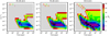 |
Fig. 24 Investigation of effect of temperature variation between 15 and 20 K. The panels show the projected best χ2 values in the ζ versus t plane for the P2 position for the XR (left), UR (middle) and R (right) search methods, but with a further constraint of T = 16 K, for Case 1 (fitting to abundances of CO, HCO+ and N2H+). The location of the minimum χ2 is marked with a white cross in each panel. |
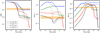 |
Fig. 25 Effects of CR induced desorption (CRID). Time evolution of the abundances of the Case 1 species CO (left), HCO+ (middle) and N2H+ (right) in the models with nH = 1.0 × 105 cm−3, T = 15 K and Av = 20 mag for several different CRIRs. The dotted lines show the fiducial case in which CRID is not included. The dashed lines show the case in which CRID is included with a standard rate (see text). The horizontal bands show the observed abundances together with their uncertainties at P2. |
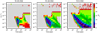 |
Fig. 26 Effects of CRID. The panels show the projected best χ2 values in the ζ versus t plane for the P2 position for the XR (left), UR (middle) and R (right) search methods using models with CRID included for Case 1 (fitting to abundances of CO, HCO+ and N2H+). The location of the minimum χ2 is marked with a white cross in each panel. Temperature is set to be 15 K for all panels. |
5.4 Combined effects and application to the full sample
Here, we examine the [CO], [HCO+] and [N2H+] data for all positions P1 to P10 and search for later time (quasi-equilibrium) models, that is in the range from t ~ 0.2 to 1 Myr, that have CRIRs that are closer to ‘standard’ values, that is ζ ~ 10−17 s−1, to see if they are able to explain the observed trends. Figure 27 shows examples of this analysis. In each row, the left panel shows fD versus nH, the middle panel shows [HCO+]/[CO] versus nH, and the right panel shows [N2H+]/[CO] versus nH. In each panel the black points show the observed data of positions P1 to P10. The grey points show the measurements assuming that 90% of the inferred [CO] is contamination from a lower density envelope (i.e. see Sect. 5.1). In general we show models for conditions with Av = 20 mag, that is a relatively high level of extinction, which should also be applicable for higher values of Av, and their results at times of 0.1, 0.2, 0.5, 1 and 2 Myr.
The first row of Fig. 27 shows models with ζ = 2.2 × 10⁻¹⁷ s−1 and with T = 15 K (solid lines) and 16 K (dotted lines). The high sensitivity of CO depletion to this choice is clearly seen. Examining the three panels, if the goal is to match the black points, then we see that this is best done at earlier times (~0.1 to 0.2 Myr), although the [HCO+]/[CO] metric is hard to match for any of the models. If the goal is to match the grey points, then this can be done with 15 K models at ages of about 0.2 to 0.5 Myr, although the N2H+ abundance can be difficult to match in the highest density sources. If the goal is to find the best later time (≳0.5 Myr) solution, then it is easiest to do when allowing for some CO envelope contamination, that is fitting to grey points, and with the 15 K models. However, overall, in all of these three cases, there is no self-consistent single solution.
The second row of Fig. 27 shows models with and without CRID included, with other parameters as in the first row for the 15 K models. If CO envelope contamination is negligible, that is attempting to fit black data points, then solutions with relatively young ages are preferred, although there is no global model that gives a good match to all the data. Similarly, if fitting to the grey data points, the models without CRID are preferred, that is the same as those found in the analysis of the first row. These are also the best later-time solutions. In summary, these ζ = 2.2 × 10⁻¹⁷ s−1 models with CRID at 15 K can only match the data if there is little CO envelope contamination and only at relatively young ages.
The third row of Fig. 27 also shows these ζ = 2.2 × 10⁻¹⁷ s−1 models with and without CRID, but now for 16 K conditions. We see from the fD results that there is little scope for CO envelope contamination in these cases and that relatively late time solutions are needed to reach even the minimum CO depletion factor estimates. However, such models tend to overproduce [HCO+] and [N2H+] abundances.
Figure 28 presents the same type of results as Fig. 27, but now for models with CRIR of ζ = 2.2 × 10⁻¹⁸ s−1. It can be seen that the effect of lowering the CRIR is to lower the abundance of HCO+ and N2H+ for a given model as a function of density and at a given age. This generally gives better agreement with the observed values of [HCO+]/[CO], and is needed for the case of no CO envelope contamination (black data points).
From a global consideration of the results of Figs. 27 and 28, we draw the following conclusions. First, we note that the observational data for fD versus density form a very tight relation, especially in comparison to what is seen in the time evolution of many of the models. We consider that this indicates that quasiequilibrium solutions that converge to this fD versus nH relation are favoured. Furthermore, this argues against there being a significant effect of CO envelope contamination, since this would be expected to introduce scatter in the fD-nH relation at about the level of the contamination factor. Late time, quasi-equilibrium solutions that match the observed fD-nH relation can be found, for example with 16 K models or with 15 K models with CRID, but to better match [HCO+] and [N2H+] constraints, then relatively low values of CRIR (≲2.2 × 10⁻¹⁸ s−1) are preferred. There is a strong sensitivity of the normalisation of the late-time, quasiequilibrium fD-nH relation to temperature occurring at values of temperature close to 15 K. While this means that agreement between the models and the data can be achieved by fine tuning the choice of temperature, again the lack of dispersion in the observational data argues against this solution. Indeed, it would favour a quasi-equilibrium solution that is insensitive to temperature, thus pointing to cosmic ray induced desorption mechanisms for liberating CO to the gas phase as being more important than simple thermal desorption. In the next subsection we consider a chemical network with revised CO ice binding energy and CRID parameters that can yield a reasonable match to the observed constraints, that is with later time solutions that converge on the observed fD-nH relation and that are insensitive to temperature for values below ~15 K.
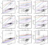 |
Fig. 27 Exploration of Case 1 fitting of the whole IRDC clump sample, including trends with density. Left column panels show fD versus nH; middle column panels show [HCO+]/[CO] versus nH; right column panels show [N2H+]/[CO] versus nH. In all panels, the black points are the observed data, while grey points assume CO envelope contamination of 90% (see text). (a) First row: temperature comparison; models have ζ = 2.2 × 10⁻¹⁷ s−1, Av = 20 mag. Solid lines are from the models with T = 15 K and dotted lines from those of T = 16 K. (b) Second row: CRID comparison at 15 K; models have ζ = 2.2 × 10⁻¹⁷ s−1, Av = 20 mag and T = 15 K. Solid lines are from the models without CRID; dotted lines are with CRID. (c) Third row: CRID comparison at 16 K; results as (b), but with T = 16 K. |
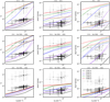 |
Fig. 28 Same as Fig. 27, but with all models having ζ = 2.2 × 10¹⁸ s−1. (a) Top row; (b) middle row; (c) bottom row. |
5.5 Models with revised astrochemical parameters of CO ice binding energy and Tcrid
In the models we have investigated so far, CO ice binding energy was set to the fiducial value of 855 K, leading to a strong sensitivity of CO depletion to temperature variation between 15 and 16 K. While this value of binding energy is suitable for pure CO ice (Öberg et al. 2005), in more realistic situations in which CO is mixed with water ice, its binding energy is expected to increase, with values of ~1100 K preferred (Öberg et al. 2005; Cuppen et al. 2017). As shown in Fig. 29, by increasing CO ice binding energy to 1100 K, CO abundance variation between 13 and 16 K becomes negligible, that is the gas phase abundance of CO decreases rapidly towards very low values. Thus, to release CO and raise its later-time gas phase abundance closer to observed levels for temperatures in the observed range ≲15 K, we need to rely on CRID.
In the astrochemical network, the main parameter which affects significantly the final CRID rate is TcriD, which is the maximum temperature reached by grains after suffering a CR impact. Within the network utilised so far, the fiducial value of Tcrid = 70 K. Figure 30 shows the effect of varying Tcrid from 70 to 100 K. We see that values of Tcrid ~ 90 to 100 K are able to sustain CO depletion factors of about 10 for relatively long timescales, up to ~10 Myr. Furthermore, as illustrated in Fig. 31, in these models the level of CO abundance around the timescales from 0.5 to 10 Myr also depends on the level of CRIR.
Figure 32 shows examples of XR fitting of P2 for a grid of models with CO ice binding energy of 1100 K and Tcrid = 100 K, that is ‘Grid 2’. Relatively early time and low CRIR solutions are again found as the best overall models, although good solutions with low χ2 values are now found extending to later times at similar values of CRIR. The main difference compared to the equivalent Grid 1 results is that these later time solutions do not require much lower values of CRIR.
Now we examine again the [CO], [HCO+] and [N2H+] data for all positions P1 to P10 and search for later-time (quasiequilibrium) models with CO ice binding energy of 1100 K and different values of Tcrid. Following the format of Figs. 27 and 28, Fig. 33 shows examples of this type of analysis. In each row the left panel shows fD versus nH, the middle panel shows [HCO+]/[CO] versus nH, and the right panel shows [N2H+]/[CO] versus nH. In each panel the black points show the observed data of positions P1 to P10. The grey points show the measurements assuming that 50% of the inferred [CO] is contaminated (i.e. see Sect. 5.1). We show models for conditions with T = 15 K (although results are relatively insensitive to temperatures near this value) and Av = 20 mag and their results at times of 0.1, 0.2, 0.5, 1 and 2 Myr.
The first row of Fig. 33 presents a high CRIR case with ζ = 1.0 × 10⁻¹⁶ s−1. Matching the observed fD-nH relation with later-time solutions requires Tcrid ≃ 80 to 85 K. However, we see that these models are not good fits to the [HCO+]/[CO] and [N2H+]/[CO] data. The second row shows ζ = 1.0 × 10⁻¹⁷ s−1 models with Tcrid = 90 and 100 K (the latter being the fiducial Grid 2 value). Again, later-time solutions can match the fD-nH relation and are now seen to be closer to, but still above, the [HCO+]/[CO] and [N2H+]/[CO] constraints. The third and fourth rows bring the CRIR down to ζ = 4.6× 10⁻¹⁸s−1 and ζ = 2.2 × 10⁻¹⁸ s−1, respectively. Values of Tcrid within 100 ± 5 K are displayed. In the third row, models with an age of about 0.5 Myr with Tcrid = 95 K are a good match to the fD-nH relation with 50% CO envelope contamination and the [HCO+]/[CO] versus nH data. They are also within about a factor of two of the [N2H+]/[CO] data. Finally, in the fourth row the 0.5 Myr models with Tcrid = 105 K are a good match to all the constraints provided by the fD, [HCO+]/[CO] and [N2H+]/[CO] versus nH data (assuming 50% CO envelope contamination).
Thus the conclusion of this analysis is that relatively latetime (~0.5 Myr) solutions (i.e. much older than a local free-fall time) exist that are insensitive to the gas temperature (in the relevant range ≲15 K) requiring only modest levels of CO envelope contamination (as implied by the relatively low scatter in the fD–nH relation). However, these solutions require thermal heating of dust grain ice mantles up to Tcrid ~ 100 K. The models also imply that the cosmic ray ionisation rate is a factor a few times smaller than the canonical value of ζ = 10−17 s−1.
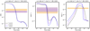 |
Fig. 29 Evolution of [CO], [HCO+] and [N2H+] in models with CO ice binding energy of 1100 K, nH = 1.0 × 105 cm−3, Av = 20mag, ζ = 1.0 × 10⁻¹⁷ s−1 and no CRID, exploring effects of different temperatures in the range relevant to IRDCs. The golden bands at each panel represent observed abundances at P2 ([HCO+] from [H13CO+]) and the purple bands show [CO] reduced by a factor of 2 (allowing for potential CO envelope contamination) and [HCO+] estimated from [HC18O+]. |
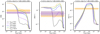 |
Fig. 30 Evolution of [CO], [HCO+] and [N2H+] in models with CO ice binding energy of 1100 K, nH = 1.0 × 105 cm−3, Av = 20 mag, ζ = 1.0 × 10⁻¹⁷ s−1 and CRID, exploring values of Tcrid from 70 to 100 K. The golden bands in each panel represent observed abundances at P2 ([HCO+] from [H13CO+]) and the purple bands show [CO] reduced by a factor of 2 (allowing for potential CO envelope contamination) and [HCO+] estimated from [HC18O+]. |
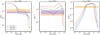 |
Fig. 31 Evolution of [CO], [HCO+] and [N2H+] in models with CO ice binding energy of 1100 K, nH = 1.0 × 105 cm−3, Av = 20 mag, Tcrid = 100 K and ζ = (0.22,0.46,1.0) × 10−17 s−1. The golden bands at each panel represent observed abundances at P2 ([HCO+] from [H13CO+]) and the purple bands show [CO] reduced by a factor of 2 (allowing for potential CO envelope contamination) and [HCO+] estimated from [HC18O+]. |
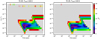 |
Fig. 32 (a) Left: example of XR Case 1 fitting of P2 abundances (HCO+ from HC18O+) using astrochemical model Grid 2 (i.e. CO ice binding energy of 1100 K and Tcrid = 100 K) showing the projected best χ2 values in the ζ versus t plane. The location of minimum χ2 is marked with a white cross. (b) Right: as (a), but now for [CO] reduced by a factor of two (allowing for potential CO envelope contamination). |
5.6 Relation to previous works and implications for massive star and star cluster formation
Summarising our results, we have found individual astrochemical models that can be a good match to observed abundances of CO, HCO+ and N2H+, that is focusing on relatively simple species that also have high sensitivity to the CRIR, implying chemical ages as short as ~105 yr, based on the timescale to freeze-out CO onto dust grains at densities of ~3 to 10 × 104 cm−3 at cold temperatures of ≲15 K. However, we have argued against such models given the relatively narrow dispersion in the observed CO depletion factor versus density relation among ten independent positions. Instead, we have concentrated on what conditions would be needed for relatively late time solutions, that is ≳3tff ~ 0.5 Myr to explain [CO], [HCO+] and [N2H+]. Here we have seen that such solutions are possible, but require an adjustment of one the main parameters involved in cosmic ray induced thermal desorption, which is Tcrid ~ 100 K, as well as favouring values of CRIR of ≲5 × 10⁻¹⁸ s−1.
One may ask how the timescale of ~ 0.5 Myr compares with expected massive star and star cluster formation times. For massive star formation from prestellar cores (PSCs) of mass Mc that are in approximate pressure equilibrium with their local clump environment that has a mass surface density of Σcl ~ 0.3 g cm−2, McKee & Tan (2003) [MT03] estimated star formation times of tf ≃ 3.2 × 10⁵(Mc/60 M⊙)1/4(Σcl/0.3 g cm−2)−3/4 yr. Thus, we see that a chemical age of ~0.5 Myr would be quite similar to the timescale expected for massive star formation in these environments, especially as the MT03 estimate is for the protostellar phase, rather than the earlier prestellar phase. For star cluster formation, the overall timescale of the process remains debated between the extremes of relatively short formation in ~ 1tff (e.g. Elmegreen 2007; Vázquez-Semadeni et al. 2019) to longer timescales of ≳10tff (e.g. Tan et al. 2006; Da Rio et al. 2014). We suggest that the lack of dispersion in the observed fD versus nH relation is evidence in favour of longer duration star formation models.
Vasyunina et al. (2012) presented astrochemical models of two IRDC positions, one estimated from NH3 observations to be cold (IRDC 013.90-1 with T ~ 13 K) and another estimated to be warm (IRDC 321.73-1 with T ~ 22 K). They included an investigation on the role of surface chemistry. They considered densities in the range nH2 = 105 to 106 cm−3, temperatures in the range T = 10 to 40 K and CRIR for H2 of 1.3 × 10⁻¹⁷ s−1. For their most complete ‘surface’ network applied to their cold IRDC, they found a most likely chemical age (based on matching to abundances of seven species) of ~105 yr, but with older ages up to about 1 Myr still having confidence parameter values within a factor of about 5 of the best value. We note that they did not have observational constraints on the abundance of CO. We consider that these results of Vasyunina et al. (2012) are broadly consistent with results that we have found, that is identifying a potential early-time solution at ~105 yr, but with later time solutions not completely excluded. However, given the significant differences in the astrochemical modelling and analysis methods, it is difficult to draw more general and definitive conclusions from this comparison.
Gerner et al. (2014) have estimated a chemical age of IRDC regions to be very short, that is ~ 104 yr. However, this is an order of magnitude shorter than the free-fall time of the regions we have considered, so seems unlikely to be valid for our case. The method of Gerner et al. (2014) is based on the time to evolve a chemical model, assuming ζ = 5 × 10⁻¹⁷ s−1 and Av = 10 mag, from its initial conditions to an observed set of abundances, but with agreement a factor of 10, and with equal weighting given to relatively complicated species whose chemistry is more uncertain). Furthermore, the possibility that the system is older is not excluded by this analysis.
Sabatini et al. (2021) studied the chemical timescales of the different phases of massive star formation, including an early 70 μm-weak phase that was inferred to have a duration of only ~5 × 10⁴ yr. However, their analysis involves several significant differences compared to our work. For example, they only considered one value of CRIR (5 × 10⁻¹⁷ s−1), one value of temperature (15 K) and one starting density (nH = 104 cm−3) for their early phase models (though they consider evolution of the density up to various values in the range 105-108 cm−3). They also focused on the relatively complicated species of CH3CCH, CH3CN, H2CO and CH3OH. Sabatini et al. (2021) described how changing the ice binding energies by ~10% leads to changes in abundances of more than one order of magnitude by the end of the evolution. Furthermore, their comparison to another chemical network (e.g. Garrod & Herbst 2006), led to order of magnitude differences in the abundances of their considered species. Given these difficulties, it appears that it is very difficult to use this type of modelling and comparison to these relatively complex species to constrain the chemical timescale of the prestellar phase with any great precision. Such considerations have led us to focus on the simpler species of CO, HCO+ and N2H+ as the primary species to be modelled.
Another general difference between our work and studies such as those of Gerner et al. (2014) and Sabatini et al. (2021) is our use of a simple one-zone model, that is of constant density, temperature, etc., rather than a more complicated model with a structured density and temperature profile. We consider that the single zone model, while approximate, is a reasonable first estimate for the average conditions in the regions traced by our molecular line observations, especially since we are focusing on the pre-stellar phase, rather than trying to model protostellar systems, which would be better described by concentrated structures with well-defined centres. While our IRDC regions likely do include higher density substructures, our modelling does allow for a range of densities to be considered above and below the average value inferred from our column density maps.
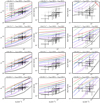 |
Fig. 33 Exploration of Case 1 fitting of the whole IRDC clump sample, including trends with density, using models with gas temperature of T = 15 K, Av = 20 mag, CO ice binding energy of 1100 K and exploring effects of cosmic ray induced desorption parameter Tcrid. Left column panels show fD versus nH; middle column panels show [HCO+]/[CO] versus nH; right column panels show [N2H+]/[CO] versus nH. In all panels, black points are the actual observed data (with HCO+ obtained from HC18O+), while the grey points assume CO abundance is reduced by a factor of 2 (due to CO envelope contamination). (a) First row: high CRIR case with ζ = 1.0 × 10⁻¹⁶ s−1. Solid lines are models with Tcrid = 80 K and dotted lines are those with Tcrid = 85 K. As shown in the legend, the various colours correspond to models from 0.1 to 2 Myr. (b) Second row: case with ζ = 1.0 × 10⁻¹⁷ s−1. Solid lines are models with Tcrid = 100 K and dotted lines are those with Tcrid = 90 K. (c) Third row: case with ζ = 4.6 × 10⁻¹⁸ s−1. Solid lines are models with Tcrid = 100 K and dotted lines are those with Tcrid = 95 K. (d) Fourth row: case with ζ = 2.2 × 10⁻¹⁸ s−1. Solid lines are models with Tcrid = 100 K and dotted lines are those with Tcrid = 105 K. |
5.7 Caveats
One potential caveat is the relative simplicity of the astrochemical modelling. In regard to the ability of the models to match [HCO+] and [N2H+] as the main constraint on CRIR, we note that in these presented models HCO+ is one of the main carriers of the positive charge, that is with [HCO+]/[e−] ~ 0.5. One may consider whether the lack of deuterated species in the astrochemical network may influence these results, especially if the deuterated species, such as H2D+ and DCO+ were to make a significant contribution to the charge budget. To examine this issue, we have considered the gas phase only deuteration modelling results of Hsu et al. (2021) with fD = 10 and similar conditions as XR for P2. We find that deuteration only makes ~20% differences to the abundance of HCO+ and so is not likely to be a major influence on our analysis.
Another caveat is the relative simplicity of the treatment of cosmic ray induced desorption. In particular, the modelling assumes a single value for the maximum temperature reached by the grains when they are hit by a cosmic ray. A more realistic treatment would allow for a distribution of such temperatures. In addition, variation of heating within an individual grain (e.g. Ivlev et al. 2015) is a feature that is also likely to be relevant and worthy of consideration in future analysis.
Finally, as discussed previously, there are a number of observational limitations. We have measured physical properties and chemical abundances averaged on scales of about 1 pc. In reality, these regions will contain a distribution of densities, temperatures, abundances, etc. In addition, a number of the regions considered are known to have sites of star formation, which will have very localised and strong variations in physical and chemical properties. While IRDCs do contain large amounts of relatively quiescent molecular gas and our study has included an effort to select regions that are free of known star formation, future studies making use of higher angular resolution data are warranted.
6 Conclusions
We have studied the astrochemical conditions in ten positions in a massive IRDC. The abundances of eight species were measured via line emission observed from single dish IRAM-30 m telescope observations, in combination with total mass surface density measurements from both Herschel dust emission and NIR+MIR extinction maps. The dust emission maps also enabled a measurement of temperature of the positions. To interpret these results an extensive grid of gas-grain astrochemical models was computed, exploring the effects of density, temperature, visual extinction of the Galactic FUV radiation field and cosmic ray ionisation rate on the time evolution of the abundances of the observed species. Furthermore, additional parameters and features of the models, which are CO ice binding energy and effect of cosmic ray induced desorption, including an exploration of the transient heating temperature, were explored.
With various restrictions on the density, temperature, and visual extinction, the standard astrochemical models (Grid 1) that best match CO, HCO+ and N2H+ (Case 1) and all species (Case 2) have been found. For Case 1 fitting, these generally favour early time solutions (i.e. t ~ 105 yr), driven by CO freeze-out timescales, and with relatively low CRIRs. However, there are islands of low χ2 at later times and higher CRIRs. Furthermore, later times can be preferable for Case 2 fittings, although with worse values of χ2.
We have discussed several aspects of the methodology that may be producing systematic errors, including the possibility of CO envelope contamination, high sensitivity to precise values of temperature near 15 K (or equivalently CO-ice binding energy assumptions) and cosmic ray induced desorption.
We have argued that the observed tightness of the CO depletion factor (fD) versus density (nH) relation argues against significant CO envelope contamination, since this would introduce significant scatter that is not observed. We have also proposed that the lack of scatter in the fD-nH relation does not favour solutions that rely on a fine tuning of temperature, but rather rely on the process of cosmic ray induced desorption to achieve a quasi-equilibrium later-time solution. Comparing to free-fall times, one would then favour models that show relatively tight, convergent behaviour after a few × tff ~ 0.3 Myr. Such a conclusion would argue against rapid evolution of the IRDC structures on timescales that are as short as their local free-fall times.
We have found that such models exist that well match the shape and normalisation of the fD-nH relation: which are the models with ζ ~ 2 to 4 × 10⁻¹⁸ s−1, Tcrid ~ 100 K, CO ice binding energy of 1100 K and ages of ~0.5 Myr (see Figs. 33c and d). Furthermore, these models also provide good matches to the observed [HCO+]/[CO] and [N2H+]/[CO] versus nH data. Within the framework of the presented models, we are not able to find good solutions with cosmic ray ionisation rates ≳few × 10−17 s−1, since these overpredict the abundances of HCO+ and N2H+. Such low rates of cosmic ray ionisation are in contrast to measurements in the diffuse ISM (e.g. Neufeld & Wolfire 2017), which may point to shielding of IRDC regions via their high column densities and∕or magnetic field gradients.
Future work to extend this type of study to other IRDCs, including in different Galactic environments, and utilising higher angular resolution molecular line observations is desirable.
Acknowledgements
We thank an anonymous referee for helpful comments that improved the paper. This work is based on that submitted in partial requirements for Ms. Negar Entekhabi’s Masters thesis in Physics at Chalmers University of Technology, supervised by Prof. Jonathan C. Tan. We acknowledge Mr. Arturo Cevallos Soto for serving as the student opponent for the Masters defense. JCT acknowldeges support from VR grant 2017-04522 and ERC project MSTAR. I.J.-S. has received partial support from the Spanish State Research Agency (AEI; project number PID2019-105552RB-C41).
References
- Barger, C. J., & Garrod, R. T. 2020, ApJ, 888, 38 [Google Scholar]
- Barnes, A., Kong, S., Tan, J., et al. 2016, MNRAS, 458, 1990 [NASA ADS] [CrossRef] [Google Scholar]
- Bron, E., Roueff, E., Gerin, M., et al. 2021, A&A, 645, A28 [NASA ADS] [CrossRef] [EDP Sciences] [Google Scholar]
- Butler, M. J., & Tan, J. C. 2009, ApJ, 696, 484 [NASA ADS] [CrossRef] [Google Scholar]
- Butler, M. J., & Tan, J. C. 2012, ApJ, 754, 5 [Google Scholar]
- Carlson, E., Profumo, S., & Linden, T. 2016, Phys. Rev. Lett., 117, 111101 [NASA ADS] [CrossRef] [Google Scholar]
- Caselli, P., Walmsley, C., Tafalla, M., Dore, L., & Myers, P. 1999, ApJ, 523, L165 [NASA ADS] [CrossRef] [Google Scholar]
- Caselli, P., Walmsley, C., Zucconi, A., et al. 2002, ApJ, 565, 344 [NASA ADS] [CrossRef] [Google Scholar]
- Ceccarelli, C., Dominik, C., López-Sepulcre, A., et al. 2014, ApJ, 790, L1 [Google Scholar]
- Crapsi, A., Caselli, P., Walmsley, M. C., & Tafalla, M. 2007, A&A, 470, 221 [NASA ADS] [CrossRef] [EDP Sciences] [Google Scholar]
- Crutcher, R. M. 2012, ARA&A, 50, 29 [Google Scholar]
- Cuppen, H., Walsh, C., Lamberts, T., et al. 2017, Space Sci. Rev., 212, 1 [NASA ADS] [CrossRef] [Google Scholar]
- Da Rio, N., Tan, J. C., & Jaehnig, K. 2014, ApJ, 795, 55 [NASA ADS] [CrossRef] [Google Scholar]
- Elmegreen, B. G. 2007, ApJ, 668, 1064 [NASA ADS] [CrossRef] [Google Scholar]
- Favre, C., Ceccarelli, C., López-Sepulcre, A., et al. 2018, ApJ, 859, 136 [Google Scholar]
- Fontani, F., Ceccarelli, C., Favre, C., et al. 2017, A&A, 605, A57 [NASA ADS] [CrossRef] [EDP Sciences] [Google Scholar]
- Gaches, B. A., & Offner, S. S. 2018, ApJ, 861, 87 [NASA ADS] [CrossRef] [Google Scholar]
- Garrod, R. T., & Herbst, E. 2006, A&A, 457, 927 [NASA ADS] [CrossRef] [EDP Sciences] [Google Scholar]
- Gerner, T., Beuther, H., Semenov, D., et al. 2014, A&A, 563, A97 [NASA ADS] [CrossRef] [EDP Sciences] [Google Scholar]
- Gieser, C., Semenov, D., Beuther, H., et al. 2019, A&A, 631, A142 [NASA ADS] [CrossRef] [EDP Sciences] [Google Scholar]
- Hasegawa, T. I., & Herbst, E. 1993, MNRAS, 261, 83 [NASA ADS] [CrossRef] [Google Scholar]
- Hernandez, A. K., Tan, J. C., Kainulainen, J., et al. 2012, ApJ, 756, L13 [NASA ADS] [CrossRef] [Google Scholar]
- Hezareh, T., Houde, M., McCoey, C., Vastel, C., & Peng, R. 2008, ApJ, 684, 1221 [NASA ADS] [CrossRef] [Google Scholar]
- Hsu, C.J., Tan, J. C., Goodson, M. D., et al. 2021, MNRAS, 502, 1104 [NASA ADS] [CrossRef] [Google Scholar]
- Ivlev, A. V., Röcker, T. B., Vasyunin, A., & Caselli, P. 2015, ApJ, 805, 59 [NASA ADS] [CrossRef] [Google Scholar]
- Jiménez-Serra, I., Caselli, P., Fontani, F., et al. 2014, MNRAS, 439, 1996 [Google Scholar]
- Kainulainen, J., & Tan, J. C. 2013, A&A, 549, A53 [NASA ADS] [CrossRef] [EDP Sciences] [Google Scholar]
- Kong, S., Tan, J. C., Caselli, P., et al. 2016, ApJ, 821, 94 [NASA ADS] [CrossRef] [Google Scholar]
- Kong, S., Arce, H. G., Maureira, M. J., et al. 2019, ApJ, 874, 104 [Google Scholar]
- Lim, W., Tan, J. C., Kainulainen, J., Ma, B., & Butler, M. J. 2016, ApJ, 829, L19 [NASA ADS] [CrossRef] [Google Scholar]
- Maffucci, D. M., Wenger, T. V., Le Gal, R., & Herbst, E. 2018, ApJ, 868, 41 [NASA ADS] [CrossRef] [Google Scholar]
- McElroy, D., Walsh, C., Markwick, A. J., et al. 2013, A&A, 550, A36 [NASA ADS] [CrossRef] [EDP Sciences] [Google Scholar]
- McKee, C. F., & Tan, J. C. 2003, ApJ, 585, 850 [Google Scholar]
- Moser, E., Liu, M., Tan, J. C., et al. 2020, ApJ, 897, 136 [NASA ADS] [CrossRef] [Google Scholar]
- Neufeld, D. A., & Wolfire, M. G. 2017, ApJ, 845, 163 [Google Scholar]
- Öberg, K., Van Broekhuizen, F., Fraser, H., et al. 2005, ApJ, 621, L33 [CrossRef] [Google Scholar]
- Padovani, M., Marcowith, A., Hennebelle, P., & Ferrière, K. 2016, A&A, 590, A8 [NASA ADS] [CrossRef] [EDP Sciences] [Google Scholar]
- Peretto, N., Fuller, G., Plume, R., et al. 2010, A&A, 518, L98 [NASA ADS] [CrossRef] [EDP Sciences] [Google Scholar]
- Pillai, T., Wyrowski, F., Carey, S. J., & Menten, K. M. 2006, A&A, 450, 569 [NASA ADS] [CrossRef] [EDP Sciences] [Google Scholar]
- Rathborne, J. M., Jackson, J., & Simon, R. 2006, ApJ, 641, 389 [NASA ADS] [CrossRef] [Google Scholar]
- Roueff, E., & Le Bourlot, J. 2020, A&A, 643, A121 [NASA ADS] [CrossRef] [EDP Sciences] [Google Scholar]
- Sabatini, G., Bovino, S., Giannetti, A., et al. 2021, A&A, 652, A71 [NASA ADS] [CrossRef] [EDP Sciences] [Google Scholar]
- Silsbee, K., Ivlev, A. V., Padovani, M., & Caselli, P. 2018, ApJ, 863, 188 [Google Scholar]
- Sipilä, O., Silsbee, K., & Caselli, P. 2021, ApJ, 922, 126 [CrossRef] [Google Scholar]
- Tan, J. C., Krumholz, M. R., & McKee, C. F. 2006, ApJ, 641, L121 [CrossRef] [Google Scholar]
- Tan, J. C., Kong, S., Butler, M. J., Caselli, P., & Fontani, F. 2013, ApJ, 779, 96 [Google Scholar]
- Tan, J. C., Beltrán, M. T., Caselli, P., et al. 2014, in Protostars and Planets VI, eds. H. Beuther, R. S. Klessen, C. P. Dullemond, & T. Henning, 149 [Google Scholar]
- Tan, J. C., Kong, S., Zhang, Y., et al. 2016, ApJ, 821, L3 [Google Scholar]
- van der Tak, F. F. S., & van Dishoeck, E. F. 2000, A&A, 358, L79 [NASA ADS] [Google Scholar]
- Vasyunina, T., Vasyunin, A. I., Herbst, E., & Linz, H. 2012, ApJ, 751, 105 [NASA ADS] [CrossRef] [Google Scholar]
- Vázquez-Semadeni, E., Palau, A., Ballesteros-Paredes, J., Gómez, G. C., & Zamora-Avilés, M. 2019, MNRAS, 490, 3061 [Google Scholar]
- Walsh, C., Millar, T., & Nomura, H. 2010, ApJ, 722, 1607 [NASA ADS] [CrossRef] [Google Scholar]
- Walsh, C., Nomura, H., Millar, T., & Aikawa, Y. 2012, ApJ, 747, 114 [NASA ADS] [CrossRef] [Google Scholar]
- Walsh, C., Millar, T., & Nomura, H. 2013, ApJ, 766, L23 [NASA ADS] [CrossRef] [Google Scholar]
- Walsh, C., Millar, T. J., Nomura, H., et al. 2014, A&A, 563, A33 [NASA ADS] [CrossRef] [EDP Sciences] [Google Scholar]
- Walsh, C., Nomura, H., & van Dishoeck, E. 2015, A&A, 582, A88 [NASA ADS] [CrossRef] [EDP Sciences] [Google Scholar]
- Wolfire, M. G., Hollenbach, D., & McKee, C. F. 2010, ApJ, 716, 1191 [Google Scholar]
- Zeng, S., Jiménez-Serra, I., Cosentino, G., et al. 2017, A&A, 603, A22 [NASA ADS] [CrossRef] [EDP Sciences] [Google Scholar]
This effect is also similar to uncertainties in the precise value of the CO-ice binding energy, which we discuss below in Sect. 5.4.
All Tables
Observed molecular species, rest frequencies, rotational quantum numbers of the transitions, rotational constants, rotational partition function, Einstein A coefficients, energy of lower state, degeneracy of upper state, velocity resolution, Beff and HPBWs.
Estimated physical properties and molecular abundances of the P1 to P10 positions in IRDC G28.37+00.07.
Extracted astrochemical parameters of the best models in R, UR and XR regions, using observed abundances of [CO],[HCO+] and [N2H+] as Case 1, and all observed abundances as Case 2.
All Figures
|
Fig. 1 Time evolution of CO depletion factor, fD, evaluated in astrochemical model Grid 1 (left column) and Grid 2 (right column) as a function of the environmental variables of: (a) top row: number density of H nuclei, nH; (b) second row: temperature, T; (c) third row: cosmic ray ionisation rate, ζ; (d) fourth row: visual extinction, Av. In each panel the three remaining variables are held fixed at their fiducial level (i.e. nH = 105 cm−3, T = 15 K, ζ = 10−17 s−1, An = 100 mag). Each time-evolving model is shown by a horizontal line with fD indicated by the colour scale. |
| In the text | |
|
Fig. 2 CO depletion factor, fD, evaluated in astrochemical model Grid 1 (dotted lines) and Grid 2 (solid lines), at fixed times of 105 (blue), 106 (green), 107 (red) and 108 yr (black) as a function of the environmental variables of: (a) top left: number density of H nuclei, nH; (b) top right: temperature, T; (c) bottom left: cosmic ray ionisation rate, ζ; (d) bottom right: visual extinction, Av. In each panel, the three remaining variables are held fixed at their fiducial level, that is nH = 105 cm−3, T = 15 K, ζ = 10−17 s−1, Av = 100 mag. |
| In the text | |
|
Fig. 3 Time evolutions of the abundances of CO (left column), HCO+ (middle column) and N2H+ (right column) evaluated in astrochemical model Grid 1 (dotted lines) and Grid 2 (solid lines), exploring the effects of the environmental variables of: (a) top row: number density of H nuclei, nH; (b) second row: temperature, T; (c) third row: cosmic ray ionisation rate, ζ; (d) bottom row: visual extinction, Av. In each row, the three remaining variables are held fixed at their fiducial level (i.e. nH = 105 cm−3, T = 15 K, ζ = 10−17 s−1, Av = 100 mag). |
| In the text | |
|
Fig. 4 (a): MIREX derived mass surface density map of IRDC G28.37+00.07 from Kainulainen & Tan (2013) (scalebar is in g cm−2). The 10 regions selected for our astrochemical study are marked with circles, labelled 1 to 10. Regions 1 to 6 (red) are known to harbour some star formation activity, while regions 7-10 have been specifically selected to avoid known protostellar sources. (b): sub-mm emission derived mass surface density map of the IRDC from Lim et al. (2016) using the Galactic Gaussian method of foreground-background subtraction (scalebar is in g cm−2). We note that it is of significantly lower angular resolution than the MIREX map (see text). The analysed positions are marked as in (a). |
| In the text | |
|
Fig. 5 Sub-mm emission derived dust temperature map of IRDC G28.37+00.07 from Lim et al. (2016) using the galactic Gaussian method of foreground-background subtraction (scalebar in K). The ten regions selected for our astrochemical study are marked with circles, labelled 1 to 10, as in Fig. 4. |
| In the text | |
|
Fig. 6 Fig. 6. – Spectra of observed species at positions P1-P5. The dashed lines indicate the velocity range 77-82 km s−1, which has been selected to cover the dense gas as traced by N2H+ and H13CO+. In the left column panels, the amplitudes of the signals of H13CO+(1-0), HC18O+ (1-0) and N2H+(1-0) have been multiplied by a factor of three for clarity of display. |
| In the text | |
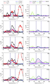 |
Fig. 7 As Fig. 6, but now for positions P6-P10. |
| In the text | |
|
Fig. 8 (a): CO depletion factor (fd) versus number density of hydrogen nuclei (nH). The data for each position are shown, along with their uncertainties. Astrochemical models are shown for ages ranging from 105 yr to 107 yr and for ζ = 10−18 s−1 (dotted lines) and 10−17 s−1 (solid lines) and 10−16 s−1 (dashed lines) with other parameters set to be T = 15 K and Av = 20 mag. (b): CO depletion factor (fd) versus visual extinction (Av). The data for each position are shown, along with their uncertainties. Astrochemical models are shown here for nH = 105 cm−3, T = 15 K and ζ = 10−17 s−1 with solid lines (colors represent different times, as in legend of (a)). An equivalent model for nH = 104 cm−3 is shown with dotted lines. |
| In the text | |
|
Fig. 9 Observed abundances of (a) CO, (b) HCO+, (c) N2H+, (d) HNC, (e) HCN, (f) HNCO, (g) H2CO and (h) CH3OH versus n∏. Astrochemical model results are also shown for ζ = 10−18 s−1 (dotted lines), 10−17 s−1 (solid lines) and 10−16 s−1 (dashed lines) with other parameters set to be T = 15 K and Av = 20 mag. |
| In the text | |
|
Fig. 10 The central panel shows the χ2 landscape (up to values of 30) in the ζ versus t plane for the P2 position for the XR search (i.e. with nH = 1.0 × 105 cm−3, Av = 20 mag and T = 15 K) Case 1 (fitting to abundances of CO, HCO+ and N2H+). The location of the minimum χ2 is marked with a white cross. The surrounding eight panels show the effect on the χ2 landscape of stepping in the model grid to the next higher and lower values of density and temperature (as labelled). Note, Av is held fixed at 20 mag in all these panels (so these are just a subset of the UR search). |
| In the text | |
|
Fig. 11 Time evolution of [CO] (gas [dotted] and ice [solid] phases) (left), [HCO+] (middle) and [N2H+] (right) for the overall best fitting model (black lines, ζ = 2.2 × 10⁻¹⁸ s−1) and best ‘late-time’ model (red lines, ζ = 2.2 × 10⁻¹⁶ s−1) for the XR search of the P2 clump, i.e. with nH = 1.0 × 105 cm−3, Av = 20 mag and T = 15 K. The time of the best models along each of these tracks is marked with a ‘+’ symbol. Horizontal dotted lines show the observed values of abundances, with the uncertainties shown by the shaded bands. |
| In the text | |
|
Fig. 12 As Fig. 11, but now showing the effect of varying the CRIR by a factor of 10 to higher (magenta) and lower (yellow) values compared to the XR best model value of ζ = 2.2 × 10⁻¹⁸ s−1. The best timescales for each of the models are shown with corresponding ‘+’ symbols, given the observed abundances of the P2 location. |
| In the text | |
|
Fig. 13 Projected best χ2 values in the ζ versus t plane for the P2 position for the XR (left), UR (middle) and R (right) search methods with Case 1 (fitting to abundances of CO, HCO+ and N2H+). The location of the minimum χ2 is marked with a white cross in each panel. |
| In the text | |
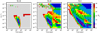 |
Fig. 14 As Fig. 13, but now for P6. |
| In the text | |
|
Fig. 15 The central panel shows the χ2 landscape (up to values of 100) in the ζ versus t plane for the P2 position for the XR search (i.e. with nH = 1.0 × 105 cm−3, Av = 20 mag and T = 15 K) Case 2 (fitting to abundances of all species). The location of the minimum χ2 is marked with a black cross. The surrounding eight panels show the effect on the χ2 landscape of stepping in the model grid to the next higher and lower values of density and temperature (as labelled). We note that Av is held fixed at 20 mag in all these panels (so these are just a subset of the UR search). |
| In the text | |
|
Fig. 16 Time evolution of [CO] (gas [dotted] and ice [solid] phases) (top left). The remaining panels show the equivalent panels for the gas phase abundances of the rest of the species for the overall best fitting model (ζ = 2.2 × 10⁻¹⁷ s−1), for the XR search of the P2 clump, that is with nH = 1.0 × 105 cm−3, Av = 20 mag and T = 15 K. The time of the best overall model along each of these tracks is marked with a ‘+’ symbol. Horizontal dotted lines show the observed values of abundances, with the uncertainties shown by the shaded bands. |
| In the text | |
|
Fig. 17 As Fig. 16, but now showing the effect of varying the CRIR by a factor of 10 to higher (magenta) and lower (yellow) values compared to the XR best model value of ζ = 2.2 × 10⁻¹⁷ s−1. The overall best timescales for each of the models are shown with corresponding ‘+’ symbols, given the observed abundances of the P2 location. |
| In the text | |
|
Fig. 18 Projected best χ2 values in the ζ versus t plane for the P2 position for the XR (left), UR (middle) and R (right) search methods with Case 2 (fitting to abundances of all species). The location of the minimum χ2 is marked with a black or white cross in each panel. |
| In the text | |
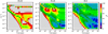 |
Fig. 19 As Fig. 18, but now for P6. |
| In the text | |
|
Fig. 20 Investigation of effect of CO envelope contamination showing the projected best χ2 values in the ζ versus t plane for the P2 position for the XR (left), UR (middle) and R (right) search methods with Case 1 (fitting to abundances of CO, HCO+ and N2H+). For this fitting, the observed abundance of CO has been reduced by a factor of 10 and the associated uncertainty is set to be a factor of 3. The location of the minimum χ2 is marked with a white cross in each panel. |
| In the text | |
|
Fig. 21 Investigation of effect of CO envelope contamination showing time evolution of [CO] (left), [HCO+] (middle) and [N2H+] (right) for the overall best fitting model (black line, ζ = 2.2 × 10⁻¹⁸ s−1). Here the observed CO abundance has been reduced by a factor of 10 and the total uncertainty set to be a factor of 3. The effects of varying the CRIR by a factor of 10 to higher (magenta) and lower (blue) values compared to the XR best model value are shown. The best timescales for each of the models are marked with corresponding ‘+’ symbols. |
| In the text | |
|
Fig. 22 Time evolution of [CO], [HCO+] and [N2H+] for XR conditions for P2, that is nH = 1 × 105 cm−3, Av =20 mag, but with various temperatures from 15 to 20 K. Here, ζ = 1.0 × 10⁻¹⁷ s−1. The horizontal band shows the observed abundances, together with corresponding uncertainties, at P2. |
| In the text | |
|
Fig. 23 Time evolution of CO, HCO+ and N2H+ abundances in the models with nH = 1 × 105 cm−3, T = 16 K, Av = 100 mag and for different values of ζ. The horizontal band shows the observed abundances together with corresponding uncertainties at P2. |
| In the text | |
|
Fig. 24 Investigation of effect of temperature variation between 15 and 20 K. The panels show the projected best χ2 values in the ζ versus t plane for the P2 position for the XR (left), UR (middle) and R (right) search methods, but with a further constraint of T = 16 K, for Case 1 (fitting to abundances of CO, HCO+ and N2H+). The location of the minimum χ2 is marked with a white cross in each panel. |
| In the text | |
|
Fig. 25 Effects of CR induced desorption (CRID). Time evolution of the abundances of the Case 1 species CO (left), HCO+ (middle) and N2H+ (right) in the models with nH = 1.0 × 105 cm−3, T = 15 K and Av = 20 mag for several different CRIRs. The dotted lines show the fiducial case in which CRID is not included. The dashed lines show the case in which CRID is included with a standard rate (see text). The horizontal bands show the observed abundances together with their uncertainties at P2. |
| In the text | |
|
Fig. 26 Effects of CRID. The panels show the projected best χ2 values in the ζ versus t plane for the P2 position for the XR (left), UR (middle) and R (right) search methods using models with CRID included for Case 1 (fitting to abundances of CO, HCO+ and N2H+). The location of the minimum χ2 is marked with a white cross in each panel. Temperature is set to be 15 K for all panels. |
| In the text | |
|
Fig. 27 Exploration of Case 1 fitting of the whole IRDC clump sample, including trends with density. Left column panels show fD versus nH; middle column panels show [HCO+]/[CO] versus nH; right column panels show [N2H+]/[CO] versus nH. In all panels, the black points are the observed data, while grey points assume CO envelope contamination of 90% (see text). (a) First row: temperature comparison; models have ζ = 2.2 × 10⁻¹⁷ s−1, Av = 20 mag. Solid lines are from the models with T = 15 K and dotted lines from those of T = 16 K. (b) Second row: CRID comparison at 15 K; models have ζ = 2.2 × 10⁻¹⁷ s−1, Av = 20 mag and T = 15 K. Solid lines are from the models without CRID; dotted lines are with CRID. (c) Third row: CRID comparison at 16 K; results as (b), but with T = 16 K. |
| In the text | |
|
Fig. 28 Same as Fig. 27, but with all models having ζ = 2.2 × 10¹⁸ s−1. (a) Top row; (b) middle row; (c) bottom row. |
| In the text | |
|
Fig. 29 Evolution of [CO], [HCO+] and [N2H+] in models with CO ice binding energy of 1100 K, nH = 1.0 × 105 cm−3, Av = 20mag, ζ = 1.0 × 10⁻¹⁷ s−1 and no CRID, exploring effects of different temperatures in the range relevant to IRDCs. The golden bands at each panel represent observed abundances at P2 ([HCO+] from [H13CO+]) and the purple bands show [CO] reduced by a factor of 2 (allowing for potential CO envelope contamination) and [HCO+] estimated from [HC18O+]. |
| In the text | |
|
Fig. 30 Evolution of [CO], [HCO+] and [N2H+] in models with CO ice binding energy of 1100 K, nH = 1.0 × 105 cm−3, Av = 20 mag, ζ = 1.0 × 10⁻¹⁷ s−1 and CRID, exploring values of Tcrid from 70 to 100 K. The golden bands in each panel represent observed abundances at P2 ([HCO+] from [H13CO+]) and the purple bands show [CO] reduced by a factor of 2 (allowing for potential CO envelope contamination) and [HCO+] estimated from [HC18O+]. |
| In the text | |
|
Fig. 31 Evolution of [CO], [HCO+] and [N2H+] in models with CO ice binding energy of 1100 K, nH = 1.0 × 105 cm−3, Av = 20 mag, Tcrid = 100 K and ζ = (0.22,0.46,1.0) × 10−17 s−1. The golden bands at each panel represent observed abundances at P2 ([HCO+] from [H13CO+]) and the purple bands show [CO] reduced by a factor of 2 (allowing for potential CO envelope contamination) and [HCO+] estimated from [HC18O+]. |
| In the text | |
|
Fig. 32 (a) Left: example of XR Case 1 fitting of P2 abundances (HCO+ from HC18O+) using astrochemical model Grid 2 (i.e. CO ice binding energy of 1100 K and Tcrid = 100 K) showing the projected best χ2 values in the ζ versus t plane. The location of minimum χ2 is marked with a white cross. (b) Right: as (a), but now for [CO] reduced by a factor of two (allowing for potential CO envelope contamination). |
| In the text | |
|
Fig. 33 Exploration of Case 1 fitting of the whole IRDC clump sample, including trends with density, using models with gas temperature of T = 15 K, Av = 20 mag, CO ice binding energy of 1100 K and exploring effects of cosmic ray induced desorption parameter Tcrid. Left column panels show fD versus nH; middle column panels show [HCO+]/[CO] versus nH; right column panels show [N2H+]/[CO] versus nH. In all panels, black points are the actual observed data (with HCO+ obtained from HC18O+), while the grey points assume CO abundance is reduced by a factor of 2 (due to CO envelope contamination). (a) First row: high CRIR case with ζ = 1.0 × 10⁻¹⁶ s−1. Solid lines are models with Tcrid = 80 K and dotted lines are those with Tcrid = 85 K. As shown in the legend, the various colours correspond to models from 0.1 to 2 Myr. (b) Second row: case with ζ = 1.0 × 10⁻¹⁷ s−1. Solid lines are models with Tcrid = 100 K and dotted lines are those with Tcrid = 90 K. (c) Third row: case with ζ = 4.6 × 10⁻¹⁸ s−1. Solid lines are models with Tcrid = 100 K and dotted lines are those with Tcrid = 95 K. (d) Fourth row: case with ζ = 2.2 × 10⁻¹⁸ s−1. Solid lines are models with Tcrid = 100 K and dotted lines are those with Tcrid = 105 K. |
| In the text | |
Current usage metrics show cumulative count of Article Views (full-text article views including HTML views, PDF and ePub downloads, according to the available data) and Abstracts Views on Vision4Press platform.
Data correspond to usage on the plateform after 2015. The current usage metrics is available 48-96 hours after online publication and is updated daily on week days.
Initial download of the metrics may take a while.