| Issue |
A&A
Volume 690, October 2024
|
|
|---|---|---|
| Article Number | A293 | |
| Number of page(s) | 13 | |
| Section | Interstellar and circumstellar matter | |
| DOI | https://doi.org/10.1051/0004-6361/202450285 | |
| Published online | 17 October 2024 | |
A new analytic approach to infer the cosmic-ray ionization rate in hot molecular cores from HCO+, N2H+, and CO observations
1
Institut de Radioastronomie Millimetrique,
300 rue de la Piscine,
38400
Saint-Martin d’Hères,
France
2
Research Center for Astronomical Computing, Zhejiang Laboratory,
Hangzhou
311100,
China
3
INAF-Osservatorio Astrofisico di Arcetri,
Largo E. Fermi 5,
50125
Firenze,
Italy
4
Department of Space, Earth and Environment, Chalmers University of Technology,
Gothenburg
412 96,
Sweden
★ Corresponding author; This email address is being protected from spambots. You need JavaScript enabled to view it.
; This email address is being protected from spambots. You need JavaScript enabled to view it.
Received:
8
April
2024
Accepted:
11
September
2024
Abstract
Context. The cosmic-ray ionization rate (ζ2) is one of the key parameters in star formation, since it regulates the chemical and dynamical evolution of molecular clouds by ionizing molecules and determining the coupling between the magnetic field and gas.
Aims. However, measurements of ζ2 in dense clouds (e.g., nH ≥ 104 cm−3) are difficult and sensitive to the model assumptions. The aim is to find a convenient analytic approach that can be used in high-mass star-forming regions (HMSFRs), especially for warm gas environments such as hot molecular cores (HMCs).
Methods. We propose a new analytic approach to calculate ζ2 through HCO+, N2H+, and CO measurements. By comparing our method with various astrochemical models and with observations found in the literature, we identify the parameter space for which the analytic approach is applicable.
Results. Our method gives a good approximation, to within 50%, of ζ2 in dense and warm gas (e.g., nH ≥ 104 cm−3, T = 50, 100 K) for AV ≥ 4 mag and t ≥ 2 × 10⁴ yr at Solar metallicity. The analytic approach gives better results for higher densities. However, it starts to underestimate ζ2 at low metallicity (Z = 0.1 Z⊙) when the value is too high (ζ2 ≥ 3 × 10⁻¹⁵ s−1). By applying our method to the OMC-2 FIR4 envelope and the L1157-B1 shock region, we find ζ2 values of (1.0 ± 0.3) × 10−14 s−1 and (2.2 ± 0.4) × 10−16 s−1, consistent with those previously reported.
Conclusions. We calculate ζ2 toward a total of 82 samples in HMSFRs, finding that the average value of ζ2 toward all HMC samples (ζ2 = (7.4±5.0)×10−16 s−1) is more than an order of magnitude higher than the theoretical prediction of cosmic-ray attenuation models, favoring the scenario that locally accelerated cosmic rays in embedded protostars should be responsible for the observed high ζ2.
Key words: astrochemistry / stars: formation / ISM: abundances / ISM: clouds / cosmic rays / ISM: molecules
© The Authors 2024
 Open Access article, published by EDP Sciences, under the terms of the Creative Commons Attribution License (https://creativecommons.org/licenses/by/4.0), which permits unrestricted use, distribution, and reproduction in any medium, provided the original work is properly cited.
This article is published in open access under the Subscribe to Open model. This email address is being protected from spambots. You need JavaScript enabled to view it. to support open access publication.
1 Introduction
Cosmic rays (CRs) play a major role in the physical and chemical evolution of dense clouds. In well-shielded regions where far-ultraviolet (FUV) photons cannot penetrate, namely where the visual extinction (AV) is larger than 3–4 mag (Wolfire et al. 2010), CRs initiate the chemistry by ionizing various molecules and producing ions (e.g., ![Mathematical equation: $\[\mathrm{H}_{3}^{+}\]$](/articles/aa/full_html/2024/10/aa50285-24/aa50285-24-eq1.png) )1. On the other hand, CRs determine the degree of ionization in dense clouds and regulate the coupling between the magnetic field and gas, which, in turn, affects the dynamic timescale during the star formation process (Dalgarno 2006; Padovani et al. 2014, 2020; Padovani & Gaches 2024).
)1. On the other hand, CRs determine the degree of ionization in dense clouds and regulate the coupling between the magnetic field and gas, which, in turn, affects the dynamic timescale during the star formation process (Dalgarno 2006; Padovani et al. 2014, 2020; Padovani & Gaches 2024).
Ions (e.g., ![Mathematical equation: $\[\mathrm{H}_{3}^{+}\]$](/articles/aa/full_html/2024/10/aa50285-24/aa50285-24-eq2.png) and HnO+) are the most favored tracers to constrain the cosmic-ray ionization rate (CRIR), since the formation and destruction of these species are relatively simple and allow us to estimate almost directly the CRIR (Gerin et al. 2010; Indriolo & McCall 2012; Indriolo et al. 2015; Neufeld & Wolfire 2017). In dense clouds, such methodology is, however, not available due to the large extinction and low abundance of the above-mentioned ions.
and HnO+) are the most favored tracers to constrain the cosmic-ray ionization rate (CRIR), since the formation and destruction of these species are relatively simple and allow us to estimate almost directly the CRIR (Gerin et al. 2010; Indriolo & McCall 2012; Indriolo et al. 2015; Neufeld & Wolfire 2017). In dense clouds, such methodology is, however, not available due to the large extinction and low abundance of the above-mentioned ions.
The abundance ratios of DCO+/HCO+ and HCO+/CO had been proposed to infer the ionization fraction and CRIR in cold prestellar cores (Caselli et al. 1998). However, the deuteration ratios are sensitive to the initial ortho-to-para ratio, the evolution timescale, and the source physical conditions (e.g., gas density and temperature, Shingledecker et al. 2016). Thus, the resultant CRIR from the above method could be overestimated by several orders of magnitude (Sabatini et al. 2023; Redaelli et al. 2024). More recently, an analytic approach using otho-H2D+ and CO was proposed to estimate the CRIR (Bovino et al. 2020) in cold prestellar cores where depletion of molecules is crucial. In addition, rovibrational H2 lines could be a potentially useful method to derive CRIR value in the cold molecular cloud (Bialy 2020; Padovani et al. 2022; Bialy et al. 2022; Gaches et al. 2022a), which would be, in principle, detected by the James Webb Space Telescope (JWST).
In high-mass star-forming regions (HMSFRs), the gas temperature increases in the more evolved phase (e.g., T ~ 100 K in hot molecular cores, HMCs, Blake et al. 1987; Beuther et al. 2007b; Luo et al. 2019; Qin et al. 2022), depletion and deuteration are inefficient, so that the methods described above cannot be adopted. Over the past decade, different molecular line tracers combined with astrochemical models have been used to probe the CRIR in HMSFRs, such as HCO+ and N2H+ (Ceccarelli et al. 2014b; Redaelli et al. 2021), and carbon-chain molecules (e.g., HC3N, HC5N, Fontani et al. 2017; Favre et al. 2018). While chemical modeling requires large computational resources, a convenient analytic approach would be useful in determining the variance of CRIR with the spatial distribution and evolution stage in HMSFRs.
In this work, we propose a new analytic approach to estimate the CRIR in HMSFRs, especially for high-mass protostellar objects (HMPOs) and HMCs. HMPOs are in a more evolved phase than the cold infrared dark cloud (IRDC). They consist of massive accreting protostars (e.g, M > 8 M⊙) and exhibit bright mid-infrared emission and strong outflows (Beuther et al. 2002b, 2007a; Zinnecker & Yorke 2007; Motte et al. 2018). The characteristic size of HMPOs is ~0.5 pc and the average density is between 104 and 106 cm−3 (Beuther et al. 2002a). HMCs appear in the later stage of HMPOs and are characterized by high gas temperatures (e.g., T ≳ 100 K), densities (nH ≳ 106 cm−3), and rich molecular lines (Blake et al. 1987; Kurtz et al. 2000; Beuther et al. 2007b; Qin et al. 2022). We compare our approach with chemical simulations from 3D-PDR and UCLCHEM and demonstrate that our method can give a good estimation of CRIR for HMPOs and HMCs.
The paper is organized as follows. We present the chemical analysis and describe the analytic approach in Sec. 2. In Sec. 3, we compare our approach with chemical simulations. We apply our method to two well-known sources and compare our results with previous modeling in the literature in Sec. 4. The uncertainties and robustness of the approach are also discussed. In Sec. 5, we calculate the CRIR toward a large sample of HMSFRs. The main results and conclusions are summarized in Sec. 6.
2 Methods
2.1 Chemical analysis
We describe, below, the formation and destruction reactions of ![Mathematical equation: $\[\mathrm{H}_{3}^{+}, \mathrm{HCO}^{+}, \mathrm{N}_{2} \mathrm{H}^{+}\]$](/articles/aa/full_html/2024/10/aa50285-24/aa50285-24-eq3.png) , and H3O+ in dense and warm clouds (e.g., nH ≥ 104 cm−3, T ≥ 50 K), where the depletion is negligible.
, and H3O+ in dense and warm clouds (e.g., nH ≥ 104 cm−3, T ≥ 50 K), where the depletion is negligible.
The formation of ![Mathematical equation: $\[\mathrm{H}_{3}^{+}\]$](/articles/aa/full_html/2024/10/aa50285-24/aa50285-24-eq4.png) in dense clouds starts from the ionization of H2 by CRs (see, e.g., Glassgold & Langer 1973):
in dense clouds starts from the ionization of H2 by CRs (see, e.g., Glassgold & Langer 1973):
![Mathematical equation: $\[\mathrm{H}_2+\mathrm{CR} \rightarrow \mathrm{H}_2^{+}+\mathrm{e}^{-},\]$](/articles/aa/full_html/2024/10/aa50285-24/aa50285-24-eq5.png) (R1)
(R1)
![Mathematical equation: $\[\mathrm{H}_2^{+}+\mathrm{H}_2 \rightarrow \mathrm{H}_3^{+}+\mathrm{H}.\]$](/articles/aa/full_html/2024/10/aa50285-24/aa50285-24-eq6.png) (R2)
(R2)
Then, ![Mathematical equation: $\[\mathrm{H}_{3}^{+}\]$](/articles/aa/full_html/2024/10/aa50285-24/aa50285-24-eq7.png) can be removed by the most abundant neutral species (Indriolo & McCall 2012):
can be removed by the most abundant neutral species (Indriolo & McCall 2012):
![Mathematical equation: $\[\begin{aligned}\mathrm{H}_3^{+}+\mathrm{CO} & \rightarrow \mathrm{HCO}^{+}+\mathrm{H}_2, \\& \rightarrow \mathrm{HOC}^{+}+\mathrm{H}_2,\end{aligned}\]$](/articles/aa/full_html/2024/10/aa50285-24/aa50285-24-eq8.png) (R3)
(R3)
![Mathematical equation: $\[\mathrm{H}_3^{+}+\mathrm{N}_2 \rightarrow \mathrm{~N}_2 \mathrm{H}^{+}+\mathrm{H}_2.\]$](/articles/aa/full_html/2024/10/aa50285-24/aa50285-24-eq9.png) (R4)
(R4)
![Mathematical equation: $\[\begin{aligned}\mathrm{H}_3^{+}+\mathrm{O} & \rightarrow \mathrm{OH}^{+}+\mathrm{H}_2, \\& \rightarrow \mathrm{H}_2 \mathrm{O}^{+}+\mathrm{H}_2,\end{aligned}\]$](/articles/aa/full_html/2024/10/aa50285-24/aa50285-24-eq10.png) (R5)
(R5)
and electrons:
![Mathematical equation: $\[\begin{aligned}\mathrm{H}_3^{+}+\mathrm{e}^{-} & \rightarrow \mathrm{H}_2+\mathrm{H}, \\& \rightarrow \mathrm{H}+\mathrm{H}+\mathrm{H}.\end{aligned}\]$](/articles/aa/full_html/2024/10/aa50285-24/aa50285-24-eq11.png) (R6)
(R6)
Reactions (R3) and (R4) are the main formation channels of HCO+2 and N2H+, respectively.
The corresponding destruction channels of HCO+ and N2H+ are (Dalgarno 2006):
![Mathematical equation: $\[\mathrm{HCO}^{+}+\mathrm{e}^{-} \rightarrow \mathrm{CO}+\mathrm{H},\]$](/articles/aa/full_html/2024/10/aa50285-24/aa50285-24-eq12.png) (R7)
(R7)
and
![Mathematical equation: $\[\mathrm{N}_2 \mathrm{H}^{+}+\mathrm{CO} \rightarrow \mathrm{HCO}^{+}+\mathrm{N}_2,\]$](/articles/aa/full_html/2024/10/aa50285-24/aa50285-24-eq13.png) (R8)
(R8)
![Mathematical equation: $\[\mathrm{N}_2 \mathrm{H}^{+}+\mathrm{e}^{-} \rightarrow \mathrm{H}+\mathrm{N}_2.\]$](/articles/aa/full_html/2024/10/aa50285-24/aa50285-24-eq14.png) (R9)
(R9)
![Mathematical equation: $\[\mathrm{N}_2 \mathrm{H}^{+}+\mathrm{O} \rightarrow \mathrm{OH}^{+}+\mathrm{N}_2.\]$](/articles/aa/full_html/2024/10/aa50285-24/aa50285-24-eq15.png) (R10)
(R10)
Considering reactions (R1)–(R6), CRIR (ζ2, referring to the ionization rate of H2) can be written as:
![Mathematical equation: $\[\zeta_2=\frac{n(\mathrm{H}_3^{+})}{n(\mathrm{H}_2)}\left[n(\mathrm{CO}) \mathrm{k}_{\mathrm{R} 3}+n\left(\mathrm{~N}_2\right) \mathrm{k}_{\mathrm{R} 4}+n(\mathrm{O}) \mathrm{k}_{\mathrm{R} 5}+n\left(\mathrm{e}^{-}\right) \mathrm{k}_{\mathrm{R} 6}\right].\]$](/articles/aa/full_html/2024/10/aa50285-24/aa50285-24-eq16.png) (1)
(1)
Similarly, from reactions (R4) and (R8)–(R10) we can write:
![Mathematical equation: $\[n(\mathrm{H}_3^{+}) n(\mathrm{~N}_2) \mathrm{k}_{\mathrm{R} 4}=n(\mathrm{~N}_2 \mathrm{H}^{+})[n(\mathrm{CO}) \mathrm{k}_{\mathrm{R} 8}+n(\mathrm{e}^{-}) \mathrm{k}_{\mathrm{R} 9}+n(\mathrm{O}) \mathrm{k}_{\mathrm{R} 10}].\]$](/articles/aa/full_html/2024/10/aa50285-24/aa50285-24-eq17.png) (2)
(2)
Considering the charge balance, the number density of electrons should be equal to the most abundant ions (see Appendix A):
![Mathematical equation: $\[n(\mathrm{e}^{-})=n(\mathrm{HCO}^{+})+n(\mathrm{N}_2 \mathrm{H}^{+})+n(\mathrm{H}_3^{+})+n(\mathrm{H}_3 \mathrm{O}^{+}).\]$](/articles/aa/full_html/2024/10/aa50285-24/aa50285-24-eq18.png) (3)
(3)
In dense clouds, the formation of H3O+ starts from reaction (R5). Then, it hydrogenates to form H2O+ and H3O+ (Bialy & Sternberg 2015; Indriolo et al. 2015; Luo et al. 2023b):
![Mathematical equation: $\[\mathrm{OH}^{+}+\mathrm{H}_2 \rightarrow \mathrm{H}_2 \mathrm{O}^{+}+\mathrm{H},\]$](/articles/aa/full_html/2024/10/aa50285-24/aa50285-24-eq19.png) (R11)
(R11)
![Mathematical equation: $\[\mathrm{H}_2 \mathrm{O}^{+}+\mathrm{H}_2 \rightarrow \mathrm{H}_3 \mathrm{O}^{+}+\mathrm{H}.\]$](/articles/aa/full_html/2024/10/aa50285-24/aa50285-24-eq20.png) (R12)
(R12)
Electron recombination reactions dominate the destruction of H3O+:
![Mathematical equation: $\[\begin{aligned}\mathrm{H}_3 \mathrm{O}^{+}+\mathrm{e}^{-} & \rightarrow \mathrm{OH}+\mathrm{H}+\mathrm{H}, \\& \rightarrow \mathrm{OH}+\mathrm{H}_2, \\& \rightarrow \mathrm{H}_2 \mathrm{O}+\mathrm{H}.\end{aligned}\]$](/articles/aa/full_html/2024/10/aa50285-24/aa50285-24-eq21.png) (R13)
(R13)
From reactions (R5), (R10), and (R11)–(R13), n(H3O+) can be written as:
![Mathematical equation: $\[n(\mathrm{H}_3 \mathrm{O}^{+})=\frac{n(\mathrm{O}) n(\mathrm{H}_3^{+}) \mathrm{k}_{\mathrm{R} 5}+n(\mathrm{~N}_2 \mathrm{H}^{+}) n(\mathrm{O}) \mathrm{k}_{\mathrm{R} 10}}{n(\mathrm{e}^{-}) \mathrm{k}_{\mathrm{R} 13}}.\]$](/articles/aa/full_html/2024/10/aa50285-24/aa50285-24-eq22.png) (4)
(4)
Combining Eqs. (3) and (4), ![Mathematical equation: $\[n\left(\mathrm{H}_{3}^{+}\right)\]$](/articles/aa/full_html/2024/10/aa50285-24/aa50285-24-eq23.png) can be written as:
can be written as:
![Mathematical equation: $\[n(\mathrm{H}_3^{+})=\frac{n(\mathrm{e}^{-})^2-n(\mathrm{e}^{-})[n(\mathrm{HCO}^{+})+n(\mathrm{~N}_2 \mathrm{H}^{+})]-\alpha}{n(\mathrm{e}^{-})+n(\mathrm{O}) \mathrm{k}_{\mathrm{R} 5} / \mathrm{k}_{\mathrm{R} 13}},\]$](/articles/aa/full_html/2024/10/aa50285-24/aa50285-24-eq24.png) (5)
(5)
where α is
![Mathematical equation: $\[\alpha=\frac{n(\mathrm{~N}_2 \mathrm{H}^{+}) n(\mathrm{O}) \mathrm{k}_{\mathrm{R} 10}}{\mathrm{k}_{\mathrm{R} 13}},\]$](/articles/aa/full_html/2024/10/aa50285-24/aa50285-24-eq25.png) (6)
(6)
Then, n(e−) can be calculated from Eqs. (2) and (5):
![Mathematical equation: $\[n(\mathrm{e}^{-})=\frac{\beta+\sqrt{\beta^2+4 \gamma \theta}}{2 \gamma},\]$](/articles/aa/full_html/2024/10/aa50285-24/aa50285-24-eq26.png) (7)
(7)
where
![Mathematical equation: $\[\begin{aligned}\beta= & \frac{n(\mathrm{N}_2 \mathrm{H}^{+})}{n(\mathrm{N}_2) \mathrm{k}_{\mathrm{R} 4}}[\frac{n(\mathrm{O}) \mathrm{k}_{\mathrm{R} 5} \mathrm{k}_{\mathrm{R} 9}}{\mathrm{k}_{\mathrm{R} 13}}+n(\mathrm{CO}) \mathrm{k}_{\mathrm{R} 8}+n(\mathrm{O}) \mathrm{k}_{\mathrm{R} 10}] \\& +n(\mathrm{HCO}^{+})+n(\mathrm{N}_2 \mathrm{H}^{+}),\end{aligned}\]$](/articles/aa/full_html/2024/10/aa50285-24/aa50285-24-eq27.png) (8)
(8)
![Mathematical equation: $\[\gamma=1-\frac{n(\mathrm{N}_2 \mathrm{H}^{+}) \mathrm{k}_{\mathrm{R} 9}}{n(\mathrm{N}_2) \mathrm{k}_{\mathrm{R} 4}},\]$](/articles/aa/full_html/2024/10/aa50285-24/aa50285-24-eq28.png) (9)
(9)
and
![Mathematical equation: $\[\theta=\alpha\left[1+\mathrm{k}_{\mathrm{R} 5} \frac{n(\mathrm{CO}) \mathrm{k}_{\mathrm{R} 8}+n(\mathrm{O}) \mathrm{k}_{\mathrm{R} 10}}{n\left(\mathrm{N}_2\right) \mathrm{k}_{\mathrm{R} 4} \mathrm{k}_{\mathrm{R} 10}}\right].\]$](/articles/aa/full_html/2024/10/aa50285-24/aa50285-24-eq29.png) (10)
(10)
To determine ζ2 through our new methodology it is needed:
a proper constraint on n(H2);
to determine the abundances of HCO+, N2H+, and CO from observations;
an assumption of the initial abundances of N2 and O.
In dense cores where hydrogen is mostly in molecular form, we can divide all number density terms (n(x)) by n(H2) in Eqs. (1)–(7). Thus, the calculated CRIR (![Mathematical equation: $\[\widetilde{\zeta}_{2}\]$](/articles/aa/full_html/2024/10/aa50285-24/aa50285-24-eq30.png) , we distinguish between the calculated CRIR (
, we distinguish between the calculated CRIR (![Mathematical equation: $\[\widetilde{\zeta}_{2}\]$](/articles/aa/full_html/2024/10/aa50285-24/aa50285-24-eq31.png) ) and the input one (ζ2) from chemical simulations) can be written as:
) and the input one (ζ2) from chemical simulations) can be written as:
![Mathematical equation: $\[\widetilde{\zeta_2}=n(\mathrm{H}_2) f(\mathrm{H}_3^{+})[f(\mathrm{CO}) \mathrm{k}_{\mathrm{R} 3}+f(\mathrm{~N}_2) \mathrm{k}_{\mathrm{R} 4}+f(\mathrm{O}) \mathrm{k}_{\mathrm{R} 5}+f(\mathrm{e}^{-}) \mathrm{k}_{\mathrm{R} 6}],\]$](/articles/aa/full_html/2024/10/aa50285-24/aa50285-24-eq32.png) (11)
(11)
where f(x) is the relative abundance of species “x” with respect to H2, n(H2) is the number density of H2, and f(e−) can be obtained from Eq. (7). For the calculations of ![Mathematical equation: $\[\widetilde{\zeta_{2}}\]$](/articles/aa/full_html/2024/10/aa50285-24/aa50285-24-eq33.png) , we use the latest reaction rates from the UMIST database (hereafter, UMIST2022, Millar et al. 2024) unless otherwise stated.
, we use the latest reaction rates from the UMIST database (hereafter, UMIST2022, Millar et al. 2024) unless otherwise stated.
2.2 Chemical models
To explore the behavior of our analytic approach, we employ the publicly available astrochemical codes3 3D-PDR (Bisbas et al. 2012) and UCLCHEM (Holdship et al. 2017). 3D-DPR is a photodissociation region code that models one- and three-dimensional density distributions. It calculates the attenuation of the FUV radiation field in every depth point and outputs the self-consistent solutions of chemical abundances, gas and dust temperature, emissivities, and level populations by performing iterations over thermal balance. In the 3D-PDR models, we consider more than 200 species with 3000 reactions taken from the UMIST20124 (McElroy et al. 2013). The initial gas phase abundances of different elements are listed in Table 1. We note that the initial element abundances are not expected to be the same everywhere. However, as long as the abundances of key species do not change significantly, the assumptions and conclusions in Sec. 2 remain valid (see Sect. 4.1.1 for more discussion on different metallicities). We also consider the treatment of CR attenuation incorporated into 3D-PDR, as presented in Gaches et al. (2019, 2022b). Unless otherwise stated, all 3D-PDR models presented here are calculated until the thermal balance is reached.
We perform additional simulations with UCLCHEM (Holdship et al. 2017) to test how the gas-grain reactions and depletion processes influence the results. UCLCHEM is a time-dependent astrochemical code focusing on gas-grain reactions. It considers freeze-out processes, thermal, and non-thermal desorption processes and outputs the chemical abundances at a given temperature, density, and AV. Contrary to 3D-PDR calculations where the code terminates as long as the thermal balance is reached, the simulations in UCLCHEM are isothermal. We set three temperatures in these simulations, Tk = 15, 50, and 100 K. The typical temperature of the cold dark cloud is 15 K and it is below the temperature for CO desorption (T ~ 20 K) (Öberg et al. 2011). The second chosen temperature (50 K) is above the sublimation temperature of simple molecules (e.g., CO) but below the desorption temperature of water ice and COMs. The third chosen temperature (100 K) is the typical temperature of HMCs and most of the species would be released from the ice phase (van Dishoeck 2014).
In UCLCHEM simulations, the deuterium chemical network of Majumdar et al. (2017) is adopted. To reduce the computational expense, species with molecular weight higher than 66 were excluded (mostly carbon-chain molecules and complex organic molecules that contain more than 5 carbon atoms). Excluding these molecules may not greatly impact the results since they gradually build up the abundances from C and C+, and have little chemical connection with the simple species we mentioned above. Besides, their abundances are usually too low (e.g., 10−10 and below, Herbst & van Dishoeck 2009) to impact the simple species. The chemical network contains a total of ~800 species and ~3 × 10⁴ reactions. The initial gas-phase abundance of HD is adopted as the value measured in the Local Bubble (1.6×10⁻⁵, Linsky et al. 2006)5. The remaining element abundances are the same as in Table 1. For all the simulations in both 3D-PDR and UCLCHEM, the cloud radius is set as 1 pc.
Initial gas-phase element abundances used in our simulations.
3 Results
3.1 Comparison to 3d-pdr simulations
We test three uniform density clouds (nH = 104, 105, and 106 cm−3) with different uniform CRIR (10−19 ≤ ζ2/s−1 ≤ 10−14) input. Figure 1 shows the ratio between CRIR derived from Eq. (11) and the input value ![Mathematical equation: $\[\left(\widetilde{\zeta}_{2} / \zeta_{2}\right)\]$](/articles/aa/full_html/2024/10/aa50285-24/aa50285-24-eq34.png) at Av = 20 mag. In most of the simulations, the calculated CRIR from the analytic approach is within 50% of the model input. The analytic approach underestimates the input CRIR by up to a factor of 3 at nH = 104 cm−3 and ζ2 = 10−14 s−1. This is due to the destruction of CO molecules under high CRIR (Bialy & Sternberg 2015; Bisbas et al. 2015, 2017), thus, the destruction pathways we analyzed in Sect. 2 change. As the density increases, the analytic approach gives a more accurate result.
at Av = 20 mag. In most of the simulations, the calculated CRIR from the analytic approach is within 50% of the model input. The analytic approach underestimates the input CRIR by up to a factor of 3 at nH = 104 cm−3 and ζ2 = 10−14 s−1. This is due to the destruction of CO molecules under high CRIR (Bialy & Sternberg 2015; Bisbas et al. 2015, 2017), thus, the destruction pathways we analyzed in Sect. 2 change. As the density increases, the analytic approach gives a more accurate result.
Figure 2 shows the deviation maps between the analytic approach and the input values at different AV and ζ2. Our analytic approach gives a good approximation, to within 50%, if ζ2 ≤ 5 × 10⁻¹⁵ s−1 and AV ≥ 4 mag at nH = 104 cm−3, and AV ≥ 4 mag for any ζ2 at nH = 105 cm−3 and nH = 106 cm−3.
In addition, we test the CR attenuation model with a variable density distribution, in which the CR spectrum is adopted as the high-energy spectrum model ℋ from Ivlev et al. (2015) and the density distribution of the cloud adopts the AV-nH relation of Bisbas et al. (2023). This relation has been found to reproduce reasonably well and at a minimal computational cost, the results from computationally expensive three-dimensional astrochemical models. Figure 3 shows the comparison between the input ζ2 and the analytical approach. At lower column densities (![Mathematical equation: $\[\left(N_{\mathrm{H}_{2}}<3.4 \times 10^{21} \mathrm{~cm}^{-2}\right.\]$](/articles/aa/full_html/2024/10/aa50285-24/aa50285-24-eq36.png) , corresponding to nH < 3 × 103 cm−3), our approach underestimates ζ2 by over 50%. At higher column densities, our approach gives a good approximation.
, corresponding to nH < 3 × 103 cm−3), our approach underestimates ζ2 by over 50%. At higher column densities, our approach gives a good approximation.
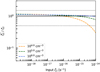 |
Fig. 1 Comparison between our approach and 3D-PDR simulations. The x-axis denotes the input CRIR of each simulation, where the CRIR in each simulation is treated as uniform. The y-axis denotes the ratio between the calculated CRIR and the input one |
![Mathematical equation: $\[\left(\widetilde{\zeta_{2}} / \zeta_{2}\right)\]$](/articles/aa/full_html/2024/10/aa50285-24/aa50285-24-eq35.png)
3.2 Comparison to UCLCHEM simulations
Figure 4 shows the comparison between the analytic approach with UCLCHEM simulations for different temperatures and densities. At low temperatures (Tk = 15 K), most of the species (including CO and O) would freeze out onto dust grain, the analytic approach underestimates the CRIR by a factor from a few (nH = 104 cm−3) to several orders of magnitude (at nH = 105 and 106 cm−3). This is expected since the depletion processes greatly reduce the abundances of CO, O, and N2 by several orders of magnitude such that the destruction pathways of ![Mathematical equation: $\[\mathrm{H}_{3}^{+}\]$](/articles/aa/full_html/2024/10/aa50285-24/aa50285-24-eq37.png) we considered in Sect. 2 (reactions (R3)–(R5)) are no longer the dominant
we considered in Sect. 2 (reactions (R3)–(R5)) are no longer the dominant ![Mathematical equation: $\[\mathrm{H}_{3}^{+}\]$](/articles/aa/full_html/2024/10/aa50285-24/aa50285-24-eq38.png) destruction mechanism. Instead, deuteration fractionation cannot be ignored such that the destruction of
destruction mechanism. Instead, deuteration fractionation cannot be ignored such that the destruction of ![Mathematical equation: $\[\mathrm{H}_{3}^{+}\]$](/articles/aa/full_html/2024/10/aa50285-24/aa50285-24-eq39.png) and the reaction channels should involve deuterated species (Millar et al. 1989; Ceccarelli et al. 2014a; Caselli et al. 2019).
and the reaction channels should involve deuterated species (Millar et al. 1989; Ceccarelli et al. 2014a; Caselli et al. 2019).
When the gas temperature is higher than the sublimation temperature of CO (the cases of Tk = 50 and 100 K), the analytic approach gives a better estimation, to within 50% for most cases. The higher the gas temperature, the better estimation is given by the analytic approach. Our analytic approach gives a more accurate estimation for higher density simulations, the same as we found with the 3D-PDR simulations.
Figure 5 shows the deviation map between the analytic approach and the input values at different evolution timescales and ζ2. For early timescales, where the molecules are still building their abundances (e.g., at nH = 104 cm−3 and t ≤ 104 yr), the analytic approach underestimates the CRIR. At nH = 104 cm−3 and t ≥ 2 × 10⁴ yr, the analytic approach gives a reasonable ζ2 estimation except for t ≈ 105 yr and ζ2 ≈ 5 × 10⁻¹⁶ s−1, where the calculated value is overestimated by a factor of 3.7. For nH = 105 cm−3, the analytic approach gives a good approximation of the CRIR for the majority of the parameter space if t > 104 yr. The maximum deviation between the analytic approach and the input value ![Mathematical equation: $\[\left(\widetilde{\zeta}_{2} / \zeta_{2}=2.6\right)\]$](/articles/aa/full_html/2024/10/aa50285-24/aa50285-24-eq40.png) appears at t ≈ 104 yr and ζ2 ≈ 5 × 10⁻¹⁵ s−1. At nH = 106 cm−3, the analytic approach gives a good estimate for all the parameter space we modeled. The results suggest that the analytic approach can be used for conditions of warm dense gas, namely in HMPOs and HMCs.
appears at t ≈ 104 yr and ζ2 ≈ 5 × 10⁻¹⁵ s−1. At nH = 106 cm−3, the analytic approach gives a good estimate for all the parameter space we modeled. The results suggest that the analytic approach can be used for conditions of warm dense gas, namely in HMPOs and HMCs.
4 Discussion
4.1 Robustness of the analytic approach
In the above simulations, we ignore the variation of initial element abundances (e.g., in different metallicity environments), the size of the source, and the gas density and temperature during the evolution processes. In the following sections, we discuss the robustness of the analytic approach under different cases.
4.1.1 Variation of metallicity
The variation of metallicity would change the initial abundances of heavy elements (heavier than He). We test three metallici-ties (Z = 0.1, 0.3, and 2 Z⊙, which correspond to low-metallicity, outer Galaxy/Large Magellanic Cloud (LMC), and the Galactic Center) with UCLCHEM at nH = 106 cm−3. The results are shown in Fig. 6. The analytic approach gives a good estimation of ζ2 at Z = 0.3 and 2 Z⊙. However, the analytic approach starts to underestimate the value of ζ2 at Z = 0.1 Z⊙ when the CRIR is high (ζ2 ≥ 3 × 10⁻¹⁵ s−1). At Z = 0.1 Z⊙, the abundances of heavy elements are reduced by a factor of 10, while the abundances of D and He remain the same. Furthermore, due to the high CRIR, key species like CO would be easily destroyed, leading to comparable or lower abundances than that of HD. Thus, the main destruction channels of ![Mathematical equation: $\[\mathrm{H}_{3}^{+}\]$](/articles/aa/full_html/2024/10/aa50285-24/aa50285-24-eq41.png) we considered in Sect. 2 would change. The results suggest that our analytic approach may only give a lower limit for metal-poor starburst galaxies where the CRIR is supposed to be extremely high.
we considered in Sect. 2 would change. The results suggest that our analytic approach may only give a lower limit for metal-poor starburst galaxies where the CRIR is supposed to be extremely high.
4.1.2 Variation of source size
In our simulations, we set the cloud radius to be 1 pc. In reality, the size of the source could change significantly in different environments. Figure 2 shows the deviation maps from 3D-PDR simulations, where the analytic approach gives a good estimation of CRIR for AV ≳ 4 mag. This value corresponds to 0.25 pc at nH = 104 cm3 and 2.5 × 10⁻³ pc (~500 AU) at nH = 106 cm−3, suggesting a minimal source size that the analytic approach can give a good CRIR estimation. We also run simulations with two different source sizes (r = 0.1, 5 pc) in UCLHEM. As seen in Fig. 7, changing the source size has no impact on the conclusions.
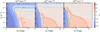 |
Fig. 2 Deviation maps between the analytic approaches and the input values at different Av and ζ2 for nH = 104 (left), 105 (middle), and 106 cm−3 (right). Red, orange, black, and blue curves denote the 20, 0, −20, and −50% deviations. |
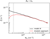 |
Fig. 3 Comparison of the calculated CRIR from the analytic approach ( |
![Mathematical equation: $\[\widetilde{\zeta}_{2}\]$](/articles/aa/full_html/2024/10/aa50285-24/aa50285-24-eq42.png)
4.1.3 HMC models
To test the robustness of our analytic approach, we perform tests with more physical HMC models, which consider both the variation of density and temperature with evolution timescale. Each of the HMC models consists of two stages. In the first stage, we perform simulations of the isothermal free-fall collapse (representing a prestellar phase) with an initial temperature of 10 K. The free-fall collapse phase starts from a cloud with nH = 103 cm−3, reaching higher densities ![Mathematical equation: $\[\left(n_{\mathrm{H}}^{\text {final }}=10^{4}, 10^{5}\right.\]$](/articles/aa/full_html/2024/10/aa50285-24/aa50285-24-eq43.png) , 105, and 106 cm−3) at a free-fall timescale6 (see Priestley et al. 2018, for a detailed description of the density profiles in collapse models). In the second stage, we perform simulations with a gradually increasing gas temperature (representing a formed HMPO or HMC) due to the heating of a central massive star. The gas densities and initial composition of all the species in the second stage inherit from the final state of the free-fall collapse. The mass of the central star in the HMC model is set to 10 M⊙, and the gas temperature increases from 10 to 200 K within a few 105 yr (see Viti et al. 2004 and Awad et al. 2010 for more details of the treatment of temperature).
, 105, and 106 cm−3) at a free-fall timescale6 (see Priestley et al. 2018, for a detailed description of the density profiles in collapse models). In the second stage, we perform simulations with a gradually increasing gas temperature (representing a formed HMPO or HMC) due to the heating of a central massive star. The gas densities and initial composition of all the species in the second stage inherit from the final state of the free-fall collapse. The mass of the central star in the HMC model is set to 10 M⊙, and the gas temperature increases from 10 to 200 K within a few 105 yr (see Viti et al. 2004 and Awad et al. 2010 for more details of the treatment of temperature).
Figure 8 shows the comparison between the analytic approach and the HMC models. The analytic approach gives a reasonable estimation for all models at ζ2 ≥ 10−17 s−1, while it underestimates ζ2 by up to a factor of 25 at ζ2 ≈ 10−18 s−1. As shown in Fig. A.1 this is due to an underestimation of electron abundance through Eq. (2) at very low CRIR, where the formation of ions (e.g., HCO+ and N2H+) is suppressed while Eq. (2) does not consider the contribution from other ions such as C+, Mg+, etc.
4.2 Uncertainties
There are a few factors that may bring uncertainties when using the analytic approach to calculate the CRIR. The most uncertain factors are the assumption of the gas phase abundances of O and N2, since they are almost undetectable in dense clouds. On the other hand, when there is a lack of measurements of CO isotopologs, a CO abundance of 10−4 (without depletion) is frequently assumed. In this section, we discuss the uncertainties induced by these factors.
Without depletion, most of the carbon is found in CO molecules in dense molecular clouds. Thus, CO has been widely used as an indicator of H2 in large surveys (Dame et al. 2001; Su et al. 2019). The canonical abundance of CO in well-shielded molecular clouds (e.g., Av > 4 mag) is ≈10−4 (Frerking et al. 1982; Pineda et al. 2010; Luo et al. 2023a). The calculated abundances of CO toward specific sightlines could also be biased by the method of deriving the column densities, excitation, and optical depths.
The abundance of molecular oxygen (O2) from both observations and chemical models is negligible compared with atomic oxygen in dense clouds (Larsson et al. 2007; Goldsmith et al. 2011; Wakelam et al. 2019). Thus, the majority of the oxygen element should be in the atomic form in dense clouds. The measured mean value of atomic oxygen abundance (with respect to total H) in the moderate density cloud (![Mathematical equation: $\[n_{\mathrm{H}_{2}}=\]$](/articles/aa/full_html/2024/10/aa50285-24/aa50285-24-eq44.png) a few 104 cm−3) is (2.51±0.69)×10−4 (Lis et al. 2023).
a few 104 cm−3) is (2.51±0.69)×10−4 (Lis et al. 2023).
Since there are no observable rotational or vibrational transitions of N2 in dense clouds, the main reservoir of nitrogen in molecular clouds is still under debate (Womack et al. 1992; Maret et al. 2006; Furuya & Persson 2018). Measurements from N2H+ in different environments suggest that N2 should be abundant in dense regions (Womack et al. 1992; Furuya & Persson 2018).
To examine the uncertainties of CRIR induced by CO and O abundances, and whether the assumed abundances of N2 are reasonable, we calculate the CRIR for each of the above chemical simulations, with the abundances (with respect to total H, including the uncertainties) of CO, O, and N2 to be (1.0 ± 0.3) × 10−4, (2.51±0.69)×l0−4, and (3.8 ± 0.5) × 10−5. Figure 9 shows the mean value (dashed lines) and 1σ deviation (shadow regions) of our analytic approach with comparison to the input ζ2 from 3D-PDR, isothermal simulations from UCLCHEM, and HMC simulations from UCLCHEM, respectively. As can be seen, the derived mean values of CRIR are mostly within 50% deviation for 3D-PDR and HMC simulations with UCLCHEM even if we consider the uncertainties induced by CO, O, and N, and the results in Sect. 3 remain the same.
Larger differences can be found in isothermal simulations with UCLCHEM. For high-temperature models (Tk = 50, 100 K) with ζ2 between 10−17 to 10−14 s−1, the mean value is consistent with that of Fig. 4 and the deviation induced by the above uncertainties are mostly within 50%. When ζ2 below a few 10−18 s−1, the deviation induced by the above uncertainties would tend to decrease the calculated CRIR by up to a factor of ~ 10. The results suggest that the assumed initial abundances of O or N2 deviate from the simulations at low CRIR. For low-temperature models (Tk = 15 K), the predicted mean value is significantly different from the previous results in Fig. 4, suggesting an unpredictable behavior at the low temperature and the analytic approach should not be used in such environments. In the following analysis, we consider all the above uncertainties when calculating the CRIR using Eq. (11).
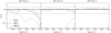 |
Fig. 4 Comparison between our approach and the UCLCHEM simulations. The x-axis denotes the input CRIR of each simulation, where the CRIR in each simulation is treated as uniform. The y-axis denotes the ratio between the calculated CRIR and the input one ( |
![Mathematical equation: $\[\widetilde{\zeta}_{2} / \zeta_{2}\]$](/articles/aa/full_html/2024/10/aa50285-24/aa50285-24-eq90.png)
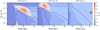 |
Fig. 5 Deviation maps between the analytic approaches and the input values at different evolution timescales and ζ2 for nH = 104 (left), 105 (middle), and 106 cm−3 (right). Red, black, and blue curves denote the 50, 0, and −50% deviations. |
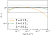 |
Fig. 6 Comparison between our approach and UCLCHEM simulations under different metallicities (Z). The temperature and density are adopted as 100 K and 106 cm−3. The solid, dash, and dotted lines represent Z = 0.1, 0.3, and 2 Z⊙. The black horizontal line represents the fiducial value and the horizontal dotted lines represent 50% of the deviation from the input values. |
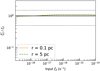 |
Fig. 7 Comparison between our approach and UCLCHEM simulations under different source size (r = 0.1 and 5 pc). The temperature and density are adopted as 100 K and 106 cm−3. The solid and dash lines represent r = 0.1 and 5 pc, respectively. The black horizontal line represents the fiducial value and the horizontal dotted lines represent 50% of the deviation from the input values. |
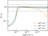 |
Fig. 8 Comparison of |
![Mathematical equation: $\[\widetilde{\zeta}_{2} / \zeta_{2}\]$](/articles/aa/full_html/2024/10/aa50285-24/aa50285-24-eq45.png)
4.3 Comparison between our calculations and the literature
We apply our method to two well-known sources (OMC-2 FIR 4 and L1157-B1) with reported CRIR values found in the literature. The two sources have available HCO+ and N2H+ observations, and the source physical properties are located within the allowable parameter space as we discussed above.
4.3.1 OMC-2 FIR4
At a distance of −420 pc (Hirota et al. 2007), OMC-2 FIR 4 is located in the north of the Orion KL object, which hosts a few embedded low- and intermediate-mass protostars (Shimajiri et al. 2008). Multi-transitions of N2H+ (J=6–5 to 12–11), HCO+ (J=6–5 to 13–12), and H13CO+ (J=6–5 to 7–6) have been observed toward this source with Herschel. The detailed spectral line energy distribution (SLED) analysis can be found in Ceccarelli et al. (2014b).
The non-local thermal equilibrium (LTE) results for the warm core component and the envelope are taken from Table 1 in Ceccarelli et al. (2014b). The column density of ![Mathematical equation: $\[\mathrm{H}_{2}\left(N_{\mathrm{H}_{2}}\right)\]$](/articles/aa/full_html/2024/10/aa50285-24/aa50285-24-eq46.png) has relatively larger uncertainties than those of molecular lines. The value of
has relatively larger uncertainties than those of molecular lines. The value of ![Mathematical equation: $\[N_{\mathrm{H}_{2}}\]$](/articles/aa/full_html/2024/10/aa50285-24/aa50285-24-eq47.png) derived from the modeled source size (~1600 AU) in Ceccarelli et al. (2014b) is 9.6×1023 cm−2. However, this value is higher than that given by radiative transfer modeling of dust spectral energy distribution (SED,
derived from the modeled source size (~1600 AU) in Ceccarelli et al. (2014b) is 9.6×1023 cm−2. However, this value is higher than that given by radiative transfer modeling of dust spectral energy distribution (SED, ![Mathematical equation: $\[N_{\mathrm{H}_{2}}=2.2 \times 10^{23} \mathrm{~cm}^{-2}\]$](/articles/aa/full_html/2024/10/aa50285-24/aa50285-24-eq48.png) , Crimier et al. 2009) and that measured from 3 mm continuum (1–9×1023 cm−2, Fontani et al. 2017). In regards to the 3 mm continuum, which could be contributed by both free-free emission and dust thermal emission, the derived
, Crimier et al. 2009) and that measured from 3 mm continuum (1–9×1023 cm−2, Fontani et al. 2017). In regards to the 3 mm continuum, which could be contributed by both free-free emission and dust thermal emission, the derived ![Mathematical equation: $\[N_{\mathrm{H}_{2}}\]$](/articles/aa/full_html/2024/10/aa50285-24/aa50285-24-eq49.png) should be considered as an upper limit.
should be considered as an upper limit.
On the other hand, due to the lack of velocity information in the dust continuum, the core and envelope components cannot be distinguished. To simplify our calculations, a median value of ![Mathematical equation: $\[N_{\mathrm{H}_{2}}=(5 \pm 1.3) \times 10^{23} \mathrm{~cm}^{-2}\]$](/articles/aa/full_html/2024/10/aa50285-24/aa50285-24-eq50.png) is adopted for the warm core component (which is the dominant component). The minimum and maximum values of
is adopted for the warm core component (which is the dominant component). The minimum and maximum values of ![Mathematical equation: $\[N_{\mathrm{H}_{2}}\]$](/articles/aa/full_html/2024/10/aa50285-24/aa50285-24-eq51.png) adopted are 1×1023 cm−2 and 9×1023 cm−2, respectively. For the envelope component, the value of
adopted are 1×1023 cm−2 and 9×1023 cm−2, respectively. For the envelope component, the value of ![Mathematical equation: $\[N_{\mathrm{H}_{2}}=6.6 \times 10^{22} \mathrm{~cm}^{-2}\]$](/articles/aa/full_html/2024/10/aa50285-24/aa50285-24-eq52.png) is adopted according to the models presented in Ceccarelli et al. (2014b).
is adopted according to the models presented in Ceccarelli et al. (2014b).
Following Eq. (11), the derived CRIR toward the warm core component is ζ2 = (1.0±0.3)×l0−14 s−1, with a lower limit of (0.6±0.2)×10−14 s−1 (adopting ![Mathematical equation: $\[N_{\mathrm{H}_{2}}=9 \times 10^{23} \mathrm{~cm}^{-2}\]$](/articles/aa/full_html/2024/10/aa50285-24/aa50285-24-eq53.png) ) and an upper limit of (5.2±1.4)×10−14 s−1 (adopting
) and an upper limit of (5.2±1.4)×10−14 s−1 (adopting ![Mathematical equation: $\[N_{\mathrm{H}_{2}}=1 \times 10^{23} \mathrm{~cm}^{-2}\]$](/articles/aa/full_html/2024/10/aa50285-24/aa50285-24-eq54.png) ). The models of Ceccarelli et al. (2014b) result in a CRIR more than two orders of magnitude higher than ours (they find ζ2 ~ 6 × 10⁻¹² s−1). We argue that this may be related to their overestimation of N2H+ and HCO+ abundances by 2~3 orders of magnitude. According to the non-LTE analysis in Ceccarelli et al. (2014b), the calculated abundances of HCO+ and N2H+ should be 7.3×10⁻¹¹ and 3.1×10⁻¹¹, respectively. However, the resultant abundances of HCO+ and N2H+ from their chemistry analysis are 10−7 and 3×10⁻⁸. The derived CRIR toward the envelope is ζ2 = (1.0±0.3)×10−14 s−1, which is slightly lower than the value given by Ceccarelli et al. (2014b, ζ2 = 1.5–8×10⁻¹⁴ s−1) and recent chemical modeling from carbon-chain molecules (ζ2 ≈ 4×10⁻¹⁴ s−1, Fontani et al. 2017; Favre et al. 2018).
). The models of Ceccarelli et al. (2014b) result in a CRIR more than two orders of magnitude higher than ours (they find ζ2 ~ 6 × 10⁻¹² s−1). We argue that this may be related to their overestimation of N2H+ and HCO+ abundances by 2~3 orders of magnitude. According to the non-LTE analysis in Ceccarelli et al. (2014b), the calculated abundances of HCO+ and N2H+ should be 7.3×10⁻¹¹ and 3.1×10⁻¹¹, respectively. However, the resultant abundances of HCO+ and N2H+ from their chemistry analysis are 10−7 and 3×10⁻⁸. The derived CRIR toward the envelope is ζ2 = (1.0±0.3)×10−14 s−1, which is slightly lower than the value given by Ceccarelli et al. (2014b, ζ2 = 1.5–8×10⁻¹⁴ s−1) and recent chemical modeling from carbon-chain molecules (ζ2 ≈ 4×10⁻¹⁴ s−1, Fontani et al. 2017; Favre et al. 2018).
4.3.2 L1157-B1
L1157-B1 is a well-known line-rich shock region, which is located at the blue-shifted outflow lobe of a low-mass protostar L1157 (Bachiller & Pérez Gutiérrez 1997; Lefloch et al. 2017; Holdship et al. 2019; Codella et al. 2020). Various molecular line emissions (e.g., CH3OH, SiO) have been detected toward L1157-B1 with broad linewidth (a few to ~20 km s−1) and enhanced abundance respect to H2. High sensitivity IRAM 30-m observations found broad linewidth (4.3 ± 0.2km s−1) emission of N2H+, while the calculated abundance of N2H+ has large uncertainties due to the unknown kinetic temperature (Codella et al. 2013; Podio et al. 2014).
Recent NH3 observations by JVLA had revealed the distribution of Tk at the blue-shifted lobe of L1157 (Feng et al. 2022). In the B1 regions, Tk is in the range of 80–120 K. We take an average Tk to be 100 K within the 26″ IRAM beam-size toward L1157-B1, and a consistent ![Mathematical equation: $\[n_{\mathrm{H}_{2}}\]$](/articles/aa/full_html/2024/10/aa50285-24/aa50285-24-eq55.png) of 105 cm−3 as in Podio et al. (2014). We use the non-local thermal equilibrium (LTE) radiative transfer model RADEX (van der Tak et al. 2007) to calculate the column density. The collisional excitation rate coefficients of N2H+ from Daniel et al. (2005) are adopted and obtained from the Leiden Atomic and Molecular Database (LAMDA, Schöier et al. 2005). The derived column density of N2H+ is (9.2 ± 1.0) × 1011 cm−2, and the resultant abundance is (9.2 ± 1.0) × 10−10. The abundances of CO and HCO+ are 1 × 10⁻⁴ and 7 × 10⁻⁹, respectively (Podio et al. 2014). The derived CRIR toward L1157-B1 from Eq. (11) is ζ2 = (2.2 ± 0.4) × 10−16 s−1, which is in good agreement with the value from chemical modeling (ζ2 ≈ 3 × 10⁻¹⁶ s−1, Podio et al. 2014; Benedettini et al. 2021).
of 105 cm−3 as in Podio et al. (2014). We use the non-local thermal equilibrium (LTE) radiative transfer model RADEX (van der Tak et al. 2007) to calculate the column density. The collisional excitation rate coefficients of N2H+ from Daniel et al. (2005) are adopted and obtained from the Leiden Atomic and Molecular Database (LAMDA, Schöier et al. 2005). The derived column density of N2H+ is (9.2 ± 1.0) × 1011 cm−2, and the resultant abundance is (9.2 ± 1.0) × 10−10. The abundances of CO and HCO+ are 1 × 10⁻⁴ and 7 × 10⁻⁹, respectively (Podio et al. 2014). The derived CRIR toward L1157-B1 from Eq. (11) is ζ2 = (2.2 ± 0.4) × 10−16 s−1, which is in good agreement with the value from chemical modeling (ζ2 ≈ 3 × 10⁻¹⁶ s−1, Podio et al. 2014; Benedettini et al. 2021).
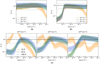 |
Fig. 9 Comparison of |
![Mathematical equation: $\[\widetilde{\zeta}_{2} / \zeta_{2}\]$](/articles/aa/full_html/2024/10/aa50285-24/aa50285-24-eq56.png)
5 The CRIR in HMSFRs
To statistically investigate how the CRIR varies in different stages of HMSFRs, we calculate CRIR using our method toward a total of 82 samples from Purcell et al. (2006, 2009) and Gerner et al. (2014, 2015). These samples include 20 HMPOs, 54 HMCs, and 8 ultra-compact H II (UCH II) regions.
In the hot core samples of Purcell et al. (2006, 2009), the gas temperatures are in the range of 28 ± 7 to 131 ± 53 K, which are derived from the rotational diagram of CH3CN. The column densities of HCO+ are derived from the optically thin H13CO+ emission, assuming 12C/13C =50 and Tex = 50 K. The column densities of N2H+ are derived from the hyperfine transitions with the assumption of Tex = 10 K and are corrected for the beam dilution with dust continuum. The column and volume densities of H2 are derived from 1.2 mm continuum emission (see Purcell et al. (2009) for details). There are no observations of CO isotopologs, in our calculation, a constant abundance of CO (1.0 ± 0.3 × 10⁻⁴) is assumed for all the hot core samples from Purcell et al. (2006, 2009).
In the samples of Gerner et al. (2014, 2015), the gas temperatures of HMPOs, HMCs, and UCH II are 29.5, 40.2, and 36 K, respectively. The column densities of HCO+ are derived from two transitions of H13CO+ (1–0 and 3–2) using RADEX, assuming 12C/13C = 897. The column densities of N2H+ are calculated with the hyperfine structure fitting routine. The column densities of CO are derived from C18O with LTE, assuming 16O/18O = 500. The H2 column densities are derived from dust emission at 850 μm with JCMT or 1.2 mm with IRAM-30 m (see Gerner et al. (2014) for details). The volume densities of H2 are derived by assuming a typical source size of 0.5 pc for all sources. We note that the choice of source size is based on the IRAM-30 m beam size, which may underestimate the actual physical size of these systems. Thus, the derived CRIR may also be underestimated.
Figure 10 shows the calculated ζ2 from the above samples. For comparison, the CRIR values from L1544 (Redaelli et al. 2021) and IRDC G28.37+00.07 (Entekhabi et al. 2022), and the theoretical CR attenuation models ℒ, ℋ, and 𝒰 from Padovani et al. (2024) are also overlaid. The models ℒ, ℋ, and 𝒰 are based on different assumptions on the low-energy slope of the interstellar CR proton spectrum (see Ivlev et al. 2015 and Padovani et al. 2024 for a detailed description of the parameterization of the CR spectrum), which have energy density ϵCR ≈ 0.65, 1.18, and 2.28 eV cm−3, respectively. The trends of the CRIR in Fig. 10 also account for the ionization due to primary and secondary electrons. It is noted that all the physical parameters ![Mathematical equation: $\[\left(T_{\text {kin }} \geq 30 \mathrm{~K}, n_{\mathrm{H}_{2}}>10^{4} \mathrm{~cm}^{-3}\right.\]$](/articles/aa/full_html/2024/10/aa50285-24/aa50285-24-eq57.png) , no CO depletion) are within the allowable parameter space that the analytic approach gives a good approximation. The average values of ζ2 in HMPOs, HMCs, and UCH II are (2.5±1.3)×10−16, (7.4±5.0)×10−16, and (3.4±3.4)×10−16 s−1, respectively. The values in these targets are over an order of magnitude higher than the measurements in prestellar cores (e.g., L1544 and G28.37+00.07) and that predicted by the model ℋ, where the latter describes the average decrease of the observationally estimated ζ2 (Padovani et al. 2022; Padovani 2023).
, no CO depletion) are within the allowable parameter space that the analytic approach gives a good approximation. The average values of ζ2 in HMPOs, HMCs, and UCH II are (2.5±1.3)×10−16, (7.4±5.0)×10−16, and (3.4±3.4)×10−16 s−1, respectively. The values in these targets are over an order of magnitude higher than the measurements in prestellar cores (e.g., L1544 and G28.37+00.07) and that predicted by the model ℋ, where the latter describes the average decrease of the observationally estimated ζ2 (Padovani et al. 2022; Padovani 2023).
Interestingly, observations from Fermi and the Large High Altitude Air Shower Observatory (LHAASO) also find the ubiquitous γ-ray emissions in HMSFRs (e.g., W43) from sub-GeV to PeV (Yang et al. 2018; Yang & Wang 2020; Vink 2022; de la Fuente et al. 2023), suggesting an efficient acceleration of particles in active star-forming environments (Bykov et al. 2020; Tibaldo et al. 2021; Owen et al. 2023). While the high energy (E ≫ 10 GeV) γ-ray could originate from CRs accelerated by stellar wind of massive stars (Peron et al. 2024), the lower energy γ-ray could come from the embedded massive protostars which undergo their accretion phase and in which the first-order Fermi acceleration mechanism operates, e.g., jet shocks (Padovani et al. 2015, 2016; Lattanzi et al. 2023), shocks on protostellar surfaces (Padovani et al. 2015, 2016; Gaches & Offner 2018), H II regions (Padovani et al. 2019; Meng et al. 2019), and wind-driven shocks (Bhadra et al. 2022). These processes would accelerate CRs to tens of GeV (depending on the actual physical conditions), leading to a detectable γ-ray emission toward individual protostar (Araudo et al. 2007; Bosch-Ramon et al. 2010; Padovani et al. 2015, 2016). The detection of γ-ray emission at ~1 GeV from the protostellar jet in HH 80–81 and ~10 GeV level toward a young massive protostar supports these scenarios (Yan et al. 2022; de Oña Wilhelmi et al. 2023).
The high values of ζ2 from our work are also consistent with the model prediction under the existence of internal CR source models as presented by Gaches et al. (2019), in which the CRIR is in the range of 10−16 s−1−10−14 s−1 at a column density of ~1023 cm−2. In addition, observations toward B335 also suggest high CRIR near the central protostars (Cabedo et al. 2023). The increasing trend of CRIR from HMPOs to HMCs is consistent with our understanding that HMCs are in a more evolved phase and that star-formation activities (e.g., shocks) in HMCs may have stronger impacts on the surrounding gas. At the late stage of HMSFRs, once the central massive protostars have gathered enough mass and evolved to the zero age main sequence, the stellar wind and radiation feedback would drive the surrounding gas and lead to an expansion of UCH II regions. And because the accretion and outflows/jets gradually disappear in the late stage, the CRIR could be lower.
Such a methodology could be, in principle, used to estimate CRIR of external galaxies, where the physical properties could be quite different to those in the Milky Way (Rosolowsky et al. 2021). However, we should note that a better understanding of the source properties (e.g., density, metallicity) and a correction for the beam dilution are needed before using such a method on distant starburst galaxies. This is because, the spatial resolution of distant galaxies is usually quite low, thus, the average volume density within the beam is not supposed to be high enough to give a good approximation at very high CRIR (ζ2 ≥ 10−14 s−1, see Sect. 3). For cosmic noon starburst galaxies where the CRIR is supposed to be extremely high (e.g., orders of magnitude above ~10−16−10−14 s−1, Indriolo et al. 2018), the analytic approach could only give a lower limit.
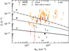 |
Fig. 10 Calculated ζ2 toward HMPOs (brown), HMCs (orange), and UCH IIs (green). Black triangles represent CRIR from IRDC G28.37+00.07, which are taken from Entekhabi et al. (2022). The cyan star represents CRIR from prestellar core L1544, which is taken from Redaelli et al. (2021). The black solid, dashed, and dash-dotted curves denote the theoretical CR attenuation models ℒ, ℋ, and 𝒰 by Padovani et al. (2024). |
6 Conclusions
We present a new analytic approach to estimate the CRIR using the abundances of HCO+, N2H+, and CO. The basic assumptions of deriving the analytic approach are: 1) ![Mathematical equation: $\[\mathrm{HCO}^{+}, \mathrm{N}_{2} \mathrm{H}^{+}, \mathrm{H}_{3}^{+}\]$](/articles/aa/full_html/2024/10/aa50285-24/aa50285-24-eq58.png) , and H3O+ are the main ions, and 2) warm gas environments (depletion of molecules can be ignored). Our analytic approach has been tested with different 3D-PDR and UCLCHEM simulations. The main conclusions are as follows:
, and H3O+ are the main ions, and 2) warm gas environments (depletion of molecules can be ignored). Our analytic approach has been tested with different 3D-PDR and UCLCHEM simulations. The main conclusions are as follows:
The analytic approach gives a reasonable estimation of ζ2 (to within 50% deviation) in dense warm gas (e.g., nH ≥ 104 cm−3, T ≥ 50 K) for Av ≥ 4 mag, t ≥ 2 × 10⁴ yr. The higher the gas density, the better the estimation from our analytic approach. Such environments may correspond to HMPOs and HMCs.
Application of our method to the OMC-2 FIR 4 envelope and L1157-B1 results in ζ2 values of (1.0 ± 0.3) × 10−14 s−1 and (2.2 ± 0.4) × 10−16 s−1, which are in good agreement with the estimation of ζ2 from the chemical modeling in the literature, suggesting wide applicability of our method in warm gas environments.
The values of ζ2 toward a total of 82 samples of HMPOs, HMCs, and UCH II have been derived with our analytic approach. The average value of ζ2 in HMCs is over an order of magnitude higher than the prediction of canonical CR attenuation models. Our results suggest that the internal massive protostars are likely to be responsible for the high CRIR.
We highlight future high spatial resolution interferometry observations with multi-transitions of molecular lines, which will allow the more robust estimation and direct mapping of CRIR in HMSFRs. This will potentially help understand the origin of the high CRIR (Padovani et al. 2019, 2021).
Acknowledgements
B.A.L.G. acknowledges support from a Chalmers Cosmic Origins postdoctoral fellowship.
Appendix A Comparison of electron fraction from our assumption and model prediction
Figure A.1 shows the comparison between the electron fraction (f(e−)) obtained from model simulations and that of Eq. 3. As can be seen, our assumption in Eq. 3 gives reasonable results for both 3D-PDR and UCLCHEM simulations. The deviation between Eq. 3 and model prediction is within a factor of ~2 for all 3D-PDR simulations and isothermal simulations from UCLCHEM. For the HMC simulations from UCLCHEM, the deviation is within a factor of 4 if 10−17 ≤ ζ2/s−1 ≤ 10−14. For ζ2 < 10−17 s−1, Eq. 3 underestimate the electron fraction since we did not consider the contribution of other ions (e.g., C+, Mg+).
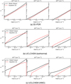 |
Fig. A.1 (a): Comparison of electron fraction as a function of ζ2 as obtained from the 3D-PDR output (black solid curves) and from Eq. 3 (red dashed curves). (b): The same as (a) while for the isothermal simulations from UCLCHEM. (c): The same as (a) while for the HMC simulations from UCLCHEM. |
Appendix B The reaction rates that appears in the analytic approach
Table B.1 lists the reaction rates that appear in Sect. 2, where the rates are taken from UMIST database (Millar et al. 2024).
References
- Araudo, A. T., Romero, G. E., Bosch-Ramon, V., & Paredes, J. M. 2007, A&A, 476, 1289 [NASA ADS] [CrossRef] [EDP Sciences] [Google Scholar]
- Awad, Z., Viti, S., Collings, M. P., & Williams, D. A. 2010, MNRAS, 407, 2511 [Google Scholar]
- Bachiller, R., & Pérez Gutiérrez, M. 1997, ApJ, 487, L93 [Google Scholar]
- Benedettini, M., Viti, S., Codella, C., et al. 2021, A&A, 645, A91 [NASA ADS] [CrossRef] [EDP Sciences] [Google Scholar]
- Beuther, H., Schilke, P., Menten, K. M., et al. 2002a, ApJ, 566, 945 [Google Scholar]
- Beuther, H., Schilke, P., Sridharan, T. K., et al. 2002b, A&A, 383, 892 [NASA ADS] [CrossRef] [EDP Sciences] [Google Scholar]
- Beuther, H., Churchwell, E. B., McKee, C. F., & Tan, J. C. 2007a, in Protostars and Planets V, eds. B. Reipurth, D. Jewitt, & K. Keil (Tucson: University of Arizona Press), 165 [Google Scholar]
- Beuther, H., Zhang, Q., Bergin, E. A., et al. 2007b, A&A, 468, 1045 [NASA ADS] [CrossRef] [EDP Sciences] [Google Scholar]
- Bhadra, S., Gupta, S., Nath, B. B., & Sharma, P. 2022, MNRAS, 510, 5579 [NASA ADS] [CrossRef] [Google Scholar]
- Bialy, S. 2020, Commun. Phys., 3, 32 [NASA ADS] [CrossRef] [Google Scholar]
- Bialy, S., & Sternberg, A. 2015, MNRAS, 450, 4424 [NASA ADS] [CrossRef] [Google Scholar]
- Bialy, S., Belli, S., & Padovani, M. 2022, A&A, 658, L13 [NASA ADS] [CrossRef] [EDP Sciences] [Google Scholar]
- Bisbas, T. G., Bell, T. A., Viti, S., Yates, J., & Barlow, M. J. 2012, MNRAS, 427, 2100 [NASA ADS] [CrossRef] [Google Scholar]
- Bisbas, T. G., Papadopoulos, P. P., & Viti, S. 2015, ApJ, 803, 37 [NASA ADS] [CrossRef] [Google Scholar]
- Bisbas, T. G., van Dishoeck, E. F., Papadopoulos, P. P., et al. 2017, ApJ, 839, 90 [Google Scholar]
- Bisbas, T. G., van Dishoeck, E. F., Hu, C.-Y., & Schruba, A. 2023, MNRAS, 519, 729 [Google Scholar]
- Blake, G. A., Sutton, E. C., Masson, C. R., & Phillips, T. G. 1987, ApJ, 315, 621 [Google Scholar]
- Bosch-Ramon, V., Romero, G. E., Araudo, A. T., & Paredes, J. M. 2010, A&A, 511, A8 [NASA ADS] [CrossRef] [EDP Sciences] [Google Scholar]
- Bovino, S., Ferrada-Chamorro, S., Lupi, A., Schleicher, D. R. G., & Caselli, P. 2020, MNRAS, 495, L7 [Google Scholar]
- Bykov, A. M., Marcowith, A., Amato, E., et al. 2020, Space Sci. Rev., 216, 42 [CrossRef] [Google Scholar]
- Cabedo, V., Maury, A., Girart, J. M., et al. 2023, A&A, 669, A90 [NASA ADS] [CrossRef] [EDP Sciences] [Google Scholar]
- Caselli, P., Walmsley, C. M., Terzieva, R., & Herbst, E. 1998, ApJ, 499, 234 [Google Scholar]
- Caselli, P., Sipilä, O., & Harju, J. 2019, arXiv e-prints [arXiv:1905.08653] [Google Scholar]
- Ceccarelli, C., Caselli, P., Bockelée-Morvan, D., et al. 2014a, in Protostars and Planets VI, eds. H. Beuther, R. S. Klessen, C. P. Dullemond, & T. Henning (Tucson: University of Arizona Press), 859 [Google Scholar]
- Ceccarelli, C., Dominik, C., López-Sepulcre, A., et al. 2014b, ApJ, 790, L1 [Google Scholar]
- Codella, C., Viti, S., Ceccarelli, C., et al. 2013, ApJ, 776, 52 [NASA ADS] [CrossRef] [Google Scholar]
- Codella, C., Ceccarelli, C., Bianchi, E., et al. 2020, A&A, 635, A17 [NASA ADS] [CrossRef] [EDP Sciences] [Google Scholar]
- Crimier, N., Ceccarelli, C., Lefloch, B., & Faure, A. 2009, A&A, 506, 1229 [NASA ADS] [CrossRef] [EDP Sciences] [Google Scholar]
- Dalgarno, A. 2006, Proc. Natl. Acad. Sci., 103, 12269 [NASA ADS] [CrossRef] [Google Scholar]
- Dame, T. M., Hartmann, D., & Thaddeus, P. 2001, ApJ, 547, 792 [Google Scholar]
- Daniel, F., Dubernet, M. L., Meuwly, M., Cernicharo, J., & Pagani, L. 2005, MNRAS, 363, 1083 [NASA ADS] [CrossRef] [Google Scholar]
- de la Fuente, E., Toledano-Juarez, I., Kawata, K., et al. 2023, PASJ, 75, 546 [NASA ADS] [CrossRef] [Google Scholar]
- de Oña Wilhelmi, E., López-Coto, R., & Su, Y. 2023, MNRAS, 523, 105 [CrossRef] [Google Scholar]
- Entekhabi, N., Tan, J. C., Cosentino, G., et al. 2022, A&A, 662, A39 [NASA ADS] [CrossRef] [EDP Sciences] [Google Scholar]
- Favre, C., Ceccarelli, C., López-Sepulcre, A., et al. 2018, ApJ, 859, 136 [Google Scholar]
- Feng, S., Liu, H. B., Caselli, P., et al. 2022, ApJ, 933, L35 [CrossRef] [Google Scholar]
- Fontani, F., Ceccarelli, C., Favre, C., et al. 2017, A&A, 605, A57 [NASA ADS] [CrossRef] [EDP Sciences] [Google Scholar]
- Frerking, M. A., Langer, W. D., & Wilson, R. W. 1982, ApJ, 262, 590 [Google Scholar]
- Friedman, S. D., Chayer, P., Jenkins, E. B., et al. 2023, ApJ, 946, 34 [NASA ADS] [CrossRef] [Google Scholar]
- Furuya, K., & Persson, M. V. 2018, MNRAS, 476, 4994 [NASA ADS] [CrossRef] [Google Scholar]
- Gaches, B. A. L., & Offner, S. S. R. 2018, ApJ, 861, 87 [NASA ADS] [CrossRef] [Google Scholar]
- Gaches, B. A. L., Offner, S. S. R., & Bisbas, T. G. 2019, ApJ, 878, 105 [NASA ADS] [CrossRef] [Google Scholar]
- Gaches, B. A. L., Bialy, S., Bisbas, T. G., et al. 2022a, A&A, 664, A150 [NASA ADS] [CrossRef] [EDP Sciences] [Google Scholar]
- Gaches, B. A. L., Bisbas, T. G., & Bialy, S. 2022b, A&A, 658, A151 [CrossRef] [EDP Sciences] [Google Scholar]
- Gerin, M., de Luca, M., Black, J., et al. 2010, A&A, 518, L110 [NASA ADS] [CrossRef] [EDP Sciences] [Google Scholar]
- Gerner, T., Beuther, H., Semenov, D., et al. 2014, A&A, 563, A97 [NASA ADS] [CrossRef] [EDP Sciences] [Google Scholar]
- Gerner, T., Shirley, Y. L., Beuther, H., et al. 2015, A&A, 579, A80 [NASA ADS] [CrossRef] [EDP Sciences] [Google Scholar]
- Glassgold, A. E., & Langer, W. D. 1973, ApJ, 179, L147 [NASA ADS] [CrossRef] [Google Scholar]
- Goldsmith, P. F., Liseau, R., Bell, T. A., et al. 2011, ApJ, 737, 96 [Google Scholar]
- Herbst, E., & van Dishoeck, E. F. 2009, ARA&A, 47, 427 [NASA ADS] [CrossRef] [Google Scholar]
- Hincelin, U., Wakelam, V., Hersant, F., et al. 2011, A&A, 530, A61 [NASA ADS] [CrossRef] [EDP Sciences] [Google Scholar]
- Hirota, T., Bushimata, T., Choi, Y. K., et al. 2007, PASJ, 59, 897 [NASA ADS] [CrossRef] [Google Scholar]
- Holdship, J., Viti, S., Jiménez-Serra, I., Makrymallis, A., & Priestley, F. 2017, AJ, 154, 38 [NASA ADS] [CrossRef] [Google Scholar]
- Holdship, J., Jimenez-Serra, I., Viti, S., et al. 2019, ApJ, 878, 64 [NASA ADS] [CrossRef] [Google Scholar]
- Indriolo, N. 2023, ApJ, 950, 64 [NASA ADS] [CrossRef] [Google Scholar]
- Indriolo, N., & McCall, B. J. 2012, ApJ, 745, 91 [NASA ADS] [CrossRef] [Google Scholar]
- Indriolo, N., Neufeld, D. A., Gerin, M., et al. 2015, ApJ, 800, 40 [NASA ADS] [CrossRef] [Google Scholar]
- Indriolo, N., Bergin, E. A., Falgarone, E., et al. 2018, ApJ, 865, 127 [NASA ADS] [CrossRef] [Google Scholar]
- Ivlev, A. V., Padovani, M., Galli, D., & Caselli, P. 2015, ApJ, 812, 135 [Google Scholar]
- Kurtz, S., Cesaroni, R., Churchwell, E., Hofner, P., & Walmsley, C. M. 2000, in Protostars and Planets IV, eds. V. Mannings, A. P. Boss, & S. S. Russell (Tucson: University of Arizona Press), 299 [Google Scholar]
- Larsson, B., Liseau, R., Pagani, L., et al. 2007, A&A, 466, 999 [NASA ADS] [CrossRef] [EDP Sciences] [Google Scholar]
- Lattanzi, V., Alves, F. O., Padovani, M., et al. 2023, A&A, 671, A35 [NASA ADS] [CrossRef] [EDP Sciences] [Google Scholar]
- Lefloch, B., Ceccarelli, C., Codella, C., et al. 2017, MNRAS, 469, L73 [Google Scholar]
- Linsky, J. L., Draine, B. T., Moos, H. W., et al. 2006, ApJ, 647, 1106 [Google Scholar]
- Lis, D. C., Goldsmith, P. F., Güsten, R., et al. 2023, A&A, 669, L15 [NASA ADS] [CrossRef] [EDP Sciences] [Google Scholar]
- Luo, G., Feng, S., Li, D., et al. 2019, ApJ, 885, 82 [NASA ADS] [CrossRef] [Google Scholar]
- Luo, G., Zhang, Z.-Y., Bisbas, T. G., et al. 2023a, ApJ, 942, 101 [NASA ADS] [CrossRef] [Google Scholar]
- Luo, G., Zhang, Z.-Y., Bisbas, T. G., et al. 2023b, ApJ, 946, 91 [NASA ADS] [CrossRef] [Google Scholar]
- Majumdar, L., Gratier, P., Ruaud, M., et al. 2017, MNRAS, 466, 4470 [Google Scholar]
- Maret, S., Bergin, E. A., & Lada, C. J. 2006, Nature, 442, 425 [Google Scholar]
- McElroy, D., Walsh, C., Markwick, A. J., et al. 2013, A&A, 550, A36 [NASA ADS] [CrossRef] [EDP Sciences] [Google Scholar]
- Meng, F., Sánchez-Monge, Á., Schilke, P., et al. 2019, A&A, 630, A73 [NASA ADS] [CrossRef] [EDP Sciences] [Google Scholar]
- Meyer, D. M., Cardelli, J. A., & Sofia, U. J. 1997, ApJ, 490, L103 [NASA ADS] [CrossRef] [Google Scholar]
- Meyer, D. M., Jura, M., & Cardelli, J. A. 1998, ApJ, 493, 222 [CrossRef] [Google Scholar]
- Milam, S. N., Savage, C., Brewster, M. A., Ziurys, L. M., & Wyckoff, S. 2005, ApJ, 634, 1126 [Google Scholar]
- Millar, T. J., Bennett, A., & Herbst, E. 1989, ApJ, 340, 906 [NASA ADS] [CrossRef] [Google Scholar]
- Millar, T. J., Walsh, C., Van de Sande, M., & Markwick, A. J. 2024, A&A, 682, A109 [NASA ADS] [CrossRef] [EDP Sciences] [Google Scholar]
- Motte, F., Bontemps, S., & Louvet, F. 2018, ARA&A, 56, 41 [NASA ADS] [CrossRef] [Google Scholar]
- Neufeld, D. A., & Wolfire, M. G. 2017, ApJ, 845, 163 [Google Scholar]
- Neufeld, D. A., Wolfire, M. G., & Schilke, P. 2005, ApJ, 628, 260 [Google Scholar]
- Öberg, K. I., Boogert, A. C. A., Pontoppidan, K. M., et al. 2011, ApJ, 740, 109 [Google Scholar]
- Owen, E. R., Wu, K., Inoue, Y., Yang, H. Y. K., & Mitchell, A. M. W. 2023, Galaxies, 11, 86 [NASA ADS] [CrossRef] [Google Scholar]
- Padovani, M. 2023, in Physics and Chemistry of Star Formation: The Dynamical ISM Across Time and Spatial Scales (Germany: Universitäts- und Stadtbibliothekj Köln), 237 [Google Scholar]
- Padovani, M., & Gaches, B. 2024, in Astrochemical Modeling: Practical Aspects of Microphysics in Numerical Simulations, eds. S. Bovino, & T., Grassi (Amsterdam: Elsevier), 189 [Google Scholar]
- Padovani, M., Galli, D., Hennebelle, P., Commerçon, B., & Joos, M. 2014, A&A, 571, A33 [NASA ADS] [CrossRef] [EDP Sciences] [Google Scholar]
- Padovani, M., Hennebelle, P., Marcowith, A., & Ferrière, K. 2015, A&A, 582, L13 [NASA ADS] [CrossRef] [EDP Sciences] [Google Scholar]
- Padovani, M., Marcowith, A., Hennebelle, P., & Ferrière, K. 2016, A&A, 590, A8 [NASA ADS] [CrossRef] [EDP Sciences] [Google Scholar]
- Padovani, M., Marcowith, A., Sánchez-Monge, Á., Meng, F., & Schilke, P. 2019, A&A, 630, A72 [NASA ADS] [CrossRef] [EDP Sciences] [Google Scholar]
- Padovani, M., Ivlev, A. V., Galli, D., et al. 2020, Space Sci. Rev., 216, 29 [CrossRef] [Google Scholar]
- Padovani, M., Marcowith, A., Galli, D., Hunt, L. K., & Fontani, F. 2021, A&A, 649, A149 [NASA ADS] [CrossRef] [EDP Sciences] [Google Scholar]
- Padovani, M., Bialy, S., Galli, D., et al. 2022, A&A, 658, A189 [NASA ADS] [CrossRef] [EDP Sciences] [Google Scholar]
- Padovani, M., Galli, D., Scarlett, L. H., et al. 2024, A&A, 682, A131 [NASA ADS] [CrossRef] [EDP Sciences] [Google Scholar]
- Peron, G., Casanova, S., Gabici, S., Baghmanyan, V., & Aharonian, F. 2024, Nat. Astron., 8, 530 [CrossRef] [Google Scholar]
- Pineda, J. L., Goldsmith, P. F., Chapman, N., et al. 2010, ApJ, 721, 686 [NASA ADS] [CrossRef] [Google Scholar]
- Podio, L., Lefloch, B., Ceccarelli, C., Codella, C., & Bachiller, R. 2014, A&A, 565, A64 [NASA ADS] [CrossRef] [EDP Sciences] [Google Scholar]
- Priestley, F. D., Viti, S., & Williams, D. A. 2018, AJ, 156, 51 [NASA ADS] [CrossRef] [Google Scholar]
- Purcell, C. R., Balasubramanyam, R., Burton, M. G., et al. 2006, MNRAS, 367, 553 [Google Scholar]
- Purcell, C. R., Longmore, S. N., Burton, M. G., et al. 2009, MNRAS, 394, 323 [NASA ADS] [CrossRef] [Google Scholar]
- Qin, S.-L., Liu, T., Liu, X., et al. 2022, MNRAS, 511, 3463 [CrossRef] [Google Scholar]
- Redaelli, E., Sipilä, O., Padovani, M., et al. 2021, A&A, 656, A109 [NASA ADS] [CrossRef] [EDP Sciences] [Google Scholar]
- Redaelli, E., Bovino, S., Lupi, A., et al. 2024, A&A, 685, A67 [NASA ADS] [CrossRef] [EDP Sciences] [Google Scholar]
- Rosolowsky, E., Hughes, A., Leroy, A. K., et al. 2021, MNRAS, 502, 1218 [NASA ADS] [CrossRef] [Google Scholar]
- Sabatini, G., Bovino, S., & Redaelli, E. 2023, ApJ, 947, L18 [NASA ADS] [CrossRef] [Google Scholar]
- Schöier, F. L., van der Tak, F. F. S., van Dishoeck, E. F., & Black, J. H. 2005, A&A, 432, 369 [Google Scholar]
- Shimajiri, Y., Takahashi, S., Takakuwa, S., Saito, M., & Kawabe, R. 2008, ApJ, 683, 255 [Google Scholar]
- Shingledecker, C. N., Bergner, J. B., Le Gal, R., et al. 2016, ApJ, 830, 151 [NASA ADS] [CrossRef] [Google Scholar]
- Sofia, U. J., Cardelli, J. A., Guerin, K. P., & Meyer, D. M. 1997, ApJ, 482, L105 [NASA ADS] [CrossRef] [Google Scholar]
- Su, Y., Yang, J., Zhang, S., et al. 2019, ApJS, 240, 9 [Google Scholar]
- Tibaldo, L., Gaggero, D., & Martin, P. 2021, Universe, 7, 141 [NASA ADS] [CrossRef] [Google Scholar]
- van der Tak, F. F. S., Black, J. H., Schöier, F. L., Jansen, D. J., & van Dishoeck, E. F. 2007, A&A, 468, 627 [NASA ADS] [CrossRef] [EDP Sciences] [Google Scholar]
- van Dishoeck, E. F. 2014, Faraday Discuss., 168, 9 [NASA ADS] [CrossRef] [Google Scholar]
- Vink, J. 2022, arXiv e-prints [arXiv:2212.10677] [Google Scholar]
- Viti, S., Collings, M. P., Dever, J. W., McCoustra, M. R. S., & Williams, D. A. 2004, MNRAS, 354, 1141 [NASA ADS] [CrossRef] [Google Scholar]
- Wakelam, V., & Herbst, E. 2008, ApJ, 680, 371 [NASA ADS] [CrossRef] [Google Scholar]
- Wakelam, V., Ruaud, M., Gratier, P., & Bonnell, I. A. 2019, MNRAS, 486, 4198 [NASA ADS] [CrossRef] [Google Scholar]
- Wolfire, M. G., Hollenbach, D., & McKee, C. F. 2010, ApJ, 716, 1191 [Google Scholar]
- Womack, M., Ziurys, L. M., & Wyckoff, S. 1992, ApJ, 393, 188 [NASA ADS] [CrossRef] [Google Scholar]
- Yan, D.-H., Zhou, J.-N., & Zhang, P.-F. 2022, Res. Astron. Astrophys., 22, 025016 [CrossRef] [Google Scholar]
- Yang, R.-Z., & Wang, Y. 2020, A&A, 640, A60 [NASA ADS] [CrossRef] [EDP Sciences] [Google Scholar]
- Yang, R.-Z., de Oña Wilhelmi, E., & Aharonian, F. 2018, A&A, 611, A77 [NASA ADS] [CrossRef] [EDP Sciences] [Google Scholar]
- Yusef-Zadeh, F., Wardle, M., Rho, J., & Sakano, M. 2003, ApJ, 585, 319 [NASA ADS] [CrossRef] [Google Scholar]
- Zinnecker, H., & Yorke, H. W. 2007, ARA&A, 45, 481 [Google Scholar]
Assuming no other sources of ionization (e.g., X-rays in the vicinity of supernova remnants, Yusef-Zadeh et al. 2003; Indriolo 2023).
Reaction (R8) below also contribute to the formation of HCO+ but with a minor role.
![Mathematical equation: $\[\widetilde{\zeta_{2}}\]$](/articles/aa/full_html/2024/10/aa50285-24/aa50285-24-eq89.png)
The measured D/H ratios in high column density regions are lower, presumably due to the depletion of D on dust grain (Linsky et al. 2006; Friedman et al. 2023). However, the D/H ratio only matters in our analysis for the dark cloud where depletion of molecules is significant (see Sec. 3.2).
The choice of the initial density would not influence the conclusion but could greatly reduce the time cost of each simulation.
Although the adopted value is higher than the local interstellar medium (ISM) (~65, Milam et al. 2005) and those from Purcell et al. (2006, 2009), a variance of 12C/13C by 30% would only result in an uncertainty of ζ2 by ~1%.
All Tables
All Figures
|
Fig. 1 Comparison between our approach and 3D-PDR simulations. The x-axis denotes the input CRIR of each simulation, where the CRIR in each simulation is treated as uniform. The y-axis denotes the ratio between the calculated CRIR and the input one |
| In the text | |
|
Fig. 2 Deviation maps between the analytic approaches and the input values at different Av and ζ2 for nH = 104 (left), 105 (middle), and 106 cm−3 (right). Red, orange, black, and blue curves denote the 20, 0, −20, and −50% deviations. |
| In the text | |
|
Fig. 3 Comparison of the calculated CRIR from the analytic approach ( |
| In the text | |
|
Fig. 4 Comparison between our approach and the UCLCHEM simulations. The x-axis denotes the input CRIR of each simulation, where the CRIR in each simulation is treated as uniform. The y-axis denotes the ratio between the calculated CRIR and the input one ( |
| In the text | |
|
Fig. 5 Deviation maps between the analytic approaches and the input values at different evolution timescales and ζ2 for nH = 104 (left), 105 (middle), and 106 cm−3 (right). Red, black, and blue curves denote the 50, 0, and −50% deviations. |
| In the text | |
|
Fig. 6 Comparison between our approach and UCLCHEM simulations under different metallicities (Z). The temperature and density are adopted as 100 K and 106 cm−3. The solid, dash, and dotted lines represent Z = 0.1, 0.3, and 2 Z⊙. The black horizontal line represents the fiducial value and the horizontal dotted lines represent 50% of the deviation from the input values. |
| In the text | |
|
Fig. 7 Comparison between our approach and UCLCHEM simulations under different source size (r = 0.1 and 5 pc). The temperature and density are adopted as 100 K and 106 cm−3. The solid and dash lines represent r = 0.1 and 5 pc, respectively. The black horizontal line represents the fiducial value and the horizontal dotted lines represent 50% of the deviation from the input values. |
| In the text | |
|
Fig. 8 Comparison of |
| In the text | |
|
Fig. 9 Comparison of |
| In the text | |
|
Fig. 10 Calculated ζ2 toward HMPOs (brown), HMCs (orange), and UCH IIs (green). Black triangles represent CRIR from IRDC G28.37+00.07, which are taken from Entekhabi et al. (2022). The cyan star represents CRIR from prestellar core L1544, which is taken from Redaelli et al. (2021). The black solid, dashed, and dash-dotted curves denote the theoretical CR attenuation models ℒ, ℋ, and 𝒰 by Padovani et al. (2024). |
| In the text | |
|
Fig. A.1 (a): Comparison of electron fraction as a function of ζ2 as obtained from the 3D-PDR output (black solid curves) and from Eq. 3 (red dashed curves). (b): The same as (a) while for the isothermal simulations from UCLCHEM. (c): The same as (a) while for the HMC simulations from UCLCHEM. |
| In the text | |
Current usage metrics show cumulative count of Article Views (full-text article views including HTML views, PDF and ePub downloads, according to the available data) and Abstracts Views on Vision4Press platform.
Data correspond to usage on the plateform after 2015. The current usage metrics is available 48-96 hours after online publication and is updated daily on week days.
Initial download of the metrics may take a while.