| Issue |
A&A
Volume 699, July 2025
|
|
|---|---|---|
| Article Number | A126 | |
| Number of page(s) | 10 | |
| Section | Interstellar and circumstellar matter | |
| DOI | https://doi.org/10.1051/0004-6361/202452470 | |
| Published online | 02 July 2025 | |
Impact of cosmic-ray propagation on the chemistry and ionisation fraction of dark clouds
1
Departamento de Astronomía, Facultad de Ciencias Físicas y Matemáticas, Universidad de Concepción, Av. Esteban Iturra s/n Barrio Universitario,
Casilla 160,
Concepción,
Chile
2
Como Lake Center for Astrophysics, DiSAT, Università degli Studi dell’Insubria,
via Valleggio 11,
22100
Como,
Italy
3
INAF, Osservatorio Astronomico di Bologna,
Via Gobetti 93/3,
40129
Bologna,
Italy
4
Chemistry Department, Sapienza University of Rome,
P.le A. Moro,
00185
Rome,
Italy
5
INAF – Osservatorio Astrofisico di Arcetri,
Largo E. Fermi 5,
50125
Firenze,
Italy
6
Max-Planck-Institut für Extraterrestrische Physik,
Giessenbachstr. 1,
85749
Garching bei München,
Germany
★ Corresponding author: This email address is being protected from spambots. You need JavaScript enabled to view it.
Received:
3
October
2024
Accepted:
30
April
2025
Abstract
Aims. A proper modelling of the cosmic-ray ionisation rate within gas clouds is crucial to describe their chemical evolution accurately. However, this modelling is computationally demanding because it requires the propagation of cosmic rays throughout the cloud over time. We present a more efficient approach that simultaneously guarantees a reliable estimate of the cosmic-ray impact on the chemistry of prestellar cores.
Methods. We introduce a numerical framework that mimics the cosmic-ray propagation within gas clouds and applies it to magnetohydrodynamic simulations performed with the code GIZMO. It simulates the cosmic-ray attenuation by computing the effective column density of H2 that is traversed, which is estimated using the same kernel weighting approach as employed in the simulation. The obtained cosmic-ray ionisation rate is then used in post-processing to study the chemical evolution of the clouds.
Results. We found that cosmic-ray propagation affects deuterated and non-deuterated species significantly and that it depends on the assumed cosmic-ray spectrum. We explored correlations between the electron abundance, the cosmic-ray ionisation rate, and the abundance of the most relevant ions (HCO+, N2H+, DCO+, N2D+, and o-H2D+), with the purpose of finding simple expressions that link them. We provide an analytical formula to estimate the ionisation fraction, X(e−), from observable tracers and applied it to existing observations of high-mass clumps. We obtained values of about 10−8, which is in line with previous works and with expectations for dense clouds. We also provide a linear fit to calculate the cosmic-ray ionisation rate from the local H2 density, which is to be employed in three-dimensional simulations that do not include cosmic-ray propagation.
Key words: ISM: abundances / ISM: clouds / cosmic rays / ISM: molecules
© The Authors 2025
 Open Access article, published by EDP Sciences, under the terms of the Creative Commons Attribution License (https://creativecommons.org/licenses/by/4.0), which permits unrestricted use, distribution, and reproduction in any medium, provided the original work is properly cited.
This article is published in open access under the Subscribe to Open model. This email address is being protected from spambots. You need JavaScript enabled to view it. to support open access publication.
1 Introduction
Dark clouds are commonly characterised by extreme conditions, such as temperatures below 20 K and high column densities that span 1023−1025 cm−2 (Bergin & Tafalla 2007). The dense material is sufficient to completely shield the cloud from incoming photo-radiation, which leaves only cosmic rays (CRs) as a potential source of ionisation in the inner regions of the clouds. Cosmic rays are non-thermal charged particles whose origin depends on their energies, which extend from local sources such as stars (109−1010 eV), galactic sources such as supernova remnants (1010−1015 eV), and extra-galactic sources such as active galactic nuclei (E > 1015 eV; see Padovani et al. 2020, as a review).
Within dark clouds, hydrogen is mainly in its molecular form, H2, and it represents the major constituent, followed by CO and then other species. Because H2 dominates the other species, CRs are expected to have a stronger impact on it and first form ![Mathematical equation: $\[\mathrm{H}_{2}^{+}\]$](/articles/aa/full_html/2025/07/aa52470-24/aa52470-24-eq1.png) and subsequently
and subsequently ![Mathematical equation: $\[\mathrm{H}_{3}^{+}\]$](/articles/aa/full_html/2025/07/aa52470-24/aa52470-24-eq2.png) . After
. After ![Mathematical equation: $\[\mathrm{H}_{3}^{+}\]$](/articles/aa/full_html/2025/07/aa52470-24/aa52470-24-eq3.png) is formed, the path to molecular formation is paved. It leads to the production of other molecules such as the OH+ and HCO+ ions (Dalgarno 2006; Indriolo & McCall 2013), the molecular form of atomic species such as O2 and N2 (Indriolo & McCall 2013), complex neutrals, H2O and NH3 (Gaches et al. 2022), and deuterated species such as H2D+ (Caselli et al. 2019).
is formed, the path to molecular formation is paved. It leads to the production of other molecules such as the OH+ and HCO+ ions (Dalgarno 2006; Indriolo & McCall 2013), the molecular form of atomic species such as O2 and N2 (Indriolo & McCall 2013), complex neutrals, H2O and NH3 (Gaches et al. 2022), and deuterated species such as H2D+ (Caselli et al. 2019).
The latter is formed through the reaction of HD with ![Mathematical equation: $\[\mathrm{H}_{3}^{+}\]$](/articles/aa/full_html/2025/07/aa52470-24/aa52470-24-eq4.png) (e.g. Dalgarno & Lepp 1984). When it is formed, the path to deuteration begins. Because H2D+ donates its deuterium atom to abundant neutral species such as CO, DCO+ is produced. At the same time, CO forms HCO+ via interaction with
(e.g. Dalgarno & Lepp 1984). When it is formed, the path to deuteration begins. Because H2D+ donates its deuterium atom to abundant neutral species such as CO, DCO+ is produced. At the same time, CO forms HCO+ via interaction with ![Mathematical equation: $\[\mathrm{H}_{3}^{+}\]$](/articles/aa/full_html/2025/07/aa52470-24/aa52470-24-eq5.png) ,
,
![Mathematical equation: $\[\mathrm{CO}+\text{o-H}_2 \mathrm{D}^{+} \longrightarrow \mathrm{DCO}^{+}+\mathrm{H}_2,\]$](/articles/aa/full_html/2025/07/aa52470-24/aa52470-24-eq6.png) (1)
(1)
![Mathematical equation: $\[\mathrm{CO}+\mathrm{H}_3^{+} \longrightarrow \mathrm{HCO}^{+}+\mathrm{H}_2.\]$](/articles/aa/full_html/2025/07/aa52470-24/aa52470-24-eq7.png) (2)
(2)
The formation of N2H+ is similar to that of HCO+,
![Mathematical equation: $\[\mathrm{N}_2+\mathrm{H}_3^{+} \longrightarrow \mathrm{N}_2 \mathrm{H}^{+}+\mathrm{H}_2.\]$](/articles/aa/full_html/2025/07/aa52470-24/aa52470-24-eq8.png) (3)
(3)
Ionisation occurs through collisions between CRs and neutral molecules (H2, N2, and CO). This drives fast ion-neutral reactions in the environment. The number of ionisations of H2 molecules (or H atoms) per unit time, referred to as the CR ionisation rate, therefore plays a fundamental role in determining the chemical state of star-forming regions. Throughout this paper, we indicate the ionisation rate for molecular hydrogen as ζ2.
Several studies have attempted to determine the CR ionisation rate from observational tracers in different environments so far, including diffuse medium (Shaw et al. 2008; Indriolo & McCall 2012), high-mass star-forming regions (Sabatini et al. 2020, 2023), circumstellar discs (Ceccarelli et al. 2014), and low-mass dense cores (Caselli et al. 1998; Redaelli et al. 2021; Bialy et al. 2022). To do this, they relied on relations between the species abundances and ζ2 (Caselli et al. 1998; Indriolo et al. 2007, 2012; Indriolo & McCall 2012; Bovino et al. 2020; Socci et al. 2024), or they explored the chemical evolution with low-dimensional (0D or 1D) models (Shaw et al. 2008; Shingledecker et al. 2016; Neufeld & Wolfire 2017; Redaelli et al. 2021). From a theoretical point of view, it is highly computationally expensive to propagate CRs in simulations alongside hydrodynamics because the particle velocities are high (close to the speed of light). This reduces the simulation time-step, the extended energy spectrum, and several uncertainties in the CR propagation process itself. Some studies have attempted to self-consistently couple CRs with magnetohydrodynamics only recently (MHD; Chan et al. 2019; Winner et al. 2019; Bustard & Zweibel 2021; Ogrodnik et al. 2021; Thomas et al. 2021), but with several limitations, and never alongside a proper nonequilibrium chemical evolution.
We explore the effect of a consistent CR propagation on the chemistry of prestellar cores simulated with the magnetohydrodynamics code GIZMO (Hopkins 2015; Hopkins & Raives 2016), which was previously reported by Bovino et al. (2019). The paper is organised as follows: In Section 2 we describe the numerical framework, that is, the CR propagator and the coupling of the CR ionisation rate to the chemical post-processing. In Section 3 we discuss our main results, and in Section 4 we draw our conclusions.
2 Numerical framework
Our numerical framework is composed of two parts, a CR propagation code that we describe in Section 2.1, and a chemical post-processing tool that we present in Section 2.2. The tool uses the output of the CR propagation code as input.
2.1 CR propagation scheme
The propagation scheme we considered aimed to mimic a continuous CR flux in which CRs are modelled as tracer particles (TPs) that propagate throughout the system (e.g. a molecular cloud). Because CRs are charged particles, they propagate along paths defined by the magnetic field lines. As CRs propagate through the cloud, they lose energy because of collisions with molecular gas. This results in an effective attenuation of the flux deeper in the cloud at increasingly higher column densities (Padovani & Gaches 2024).
The structure of the propagation scheme is as follows:
- (i)
TP generation: A specific number of TPs are created (determined by 2p, with p set before the run) at a distance R from the cloud, and they are distributed randomly over a spherical surface. The initial direction of the TPs along the magnetic field lines is chosen to be towards the centre of the cloud, and all are assumed to start from a uniform isotropic distribution of pitch angles (α0) over a hemisphere, where the pitch angle distribution ranges from 0 to π/2, sampled using Nα bins. For each initial value of the pitch angle, TPs are assigned an initial column density
![Mathematical equation: $\[N_{\mathrm{eff}}\left(\mathbf{x}_0, \alpha_0\right)=\frac{2 \times 10^{21} \mathrm{~cm}^{-2}}{\cos ~\alpha_0},\]$](/articles/aa/full_html/2025/07/aa52470-24/aa52470-24-eq9.png) (4)
(4)where Neff stands for the effective column density that is traversed by the TP, 2 × 1021 cm−2 is the column density value at which hydrogen is mainly in its molecular form (Snow & McCall 2006), and x0 is the initial position of the TP.
- (ii)
Gas particle interpolation: In order to compute the column density that is traversed by CRs and then the CR ionisation rate, local gas properties at the position of the TPs are needed, in particular, the H2 number density n(H2) and the average magnetic field B, the latter setting the propagation direction. Because all these physical quantities vary throughout the cloud, we estimated them by means of kernel weighting, analogous to what is done for hydrodynamics (see Hopkins 2015). In particular, at the location xk of the k-th TP, we determined the kernel size hk that encompasses an effective number of gas-neighbours Nngb = 32, defined by
![Mathematical equation: $\[N_{\mathrm{ngb}}=\frac{4 \pi}{3} h_k^3 \sum_j W\left(\mathbf{x}_j-\mathbf{x}_k, h_k\right),\]$](/articles/aa/full_html/2025/07/aa52470-24/aa52470-24-eq10.png) (5)
(5)where the sum is over all neighbours within hk, xj is the location of the jth neighbour, and the kernel function W(xj − xk, hk) is defined by the standard cubic spline
![Mathematical equation: $\[\bar{W}\left(q, h_k\right)=\frac{8}{\pi h_k^3} \begin{cases}1-6 q^2+6 q^3, & 0 \leq q \leq \frac{1}{2}, \\ 2(1-q)^3, & \frac{1}{2}<q \leq 1, \\ 0, & q>1,\end{cases}\]$](/articles/aa/full_html/2025/07/aa52470-24/aa52470-24-eq11.png) (6)
(6)with q = |xj − xk|/hk the normalised distance.
The neighbour search is repeated at each step of the integration for all TPs and thus represents the highest computational cost of the scheme because Eq. (5) must be solved implicitly. To limit the computational cost and rapidly converge to the desired solution, we performed this operation using a Newton-Raphson iteration1 (Springel 2005; Hopkins 2015). After the kernel size was determined, a last loop on the neighbours was performed to compute the smoothed magnetic field and the gas density, which were then used to update the column density.
- (iii)
TPs propagation: The propagation of TPs is computed by means of a fourth-order Runge-Kutta integrator, where the step size for the kth TP is determined as Δℓk = 0.1Δxk, with
![Mathematical equation: $\[\Delta x_{k}=(4 \pi / 3)^{1 / 3} N_{\text {ngb }}^{-1 / 3} h_{k}\]$](/articles/aa/full_html/2025/07/aa52470-24/aa52470-24-eq12.png) the grid-equivalent inter-particle spacing, and motion occurs along the direction of the smoothed magnetic field. We note that the interpolated quantities were recomputed at every sub-step of the propagation by repeating (ii).
the grid-equivalent inter-particle spacing, and motion occurs along the direction of the smoothed magnetic field. We note that the interpolated quantities were recomputed at every sub-step of the propagation by repeating (ii). - (iv)
Column density and CR ionisation rate update: Using the new location of the TP x′ and the new interpolated quantities n(x′) and B(x′), we updated the column density that is traversed by CRs as
![Mathematical equation: $\[N_{\mathrm{eff}}\left(\mathbf{x}^{\prime}, \alpha_0\right)=N_{\mathrm{eff}}\left(\mathbf{x}, \alpha_{\mathbf{0}}\right)+\frac{n\left(\mathbf{x}^{\prime}\right) \Delta \ell_k}{\sqrt{1-B_k\left(\mathbf{x}^{\prime}\right) \sin ^2\left(\alpha_0\right) / B_{k, 0}}},\]$](/articles/aa/full_html/2025/07/aa52470-24/aa52470-24-eq13.png) (7)
(7)and the corresponding CR ionisation rate was re-estimated by integrating with the trapezoidal rule over all the pitch angles as
![Mathematical equation: $\[\zeta_2\left(\mathbf{x}^{\prime}\right)=\delta\left(\mathbf{x}^{\prime}\right) \int_0^{\pi / 2} f\left[N_{\mathrm{eff}}\left(\mathbf{x}^{\prime}, \alpha\right)\right] \sin \alpha ~\mathrm{d} \alpha,\]$](/articles/aa/full_html/2025/07/aa52470-24/aa52470-24-eq14.png) (8)
(8)
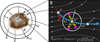
Fig. 1 Sketch of the CR propagation scheme based on the structure given in Section 2.1. The left panel describes the TP propagation through the domain. TPs (grey dots) are created from a spherical surface of radius R (dashed black circle) with radial inward trajectories (step i). TPs are then deactivated when the column density that is traversed exceeds 1029 cm−2 or when they leave the outer spherical surface at a distance Rout (solid black circle), as shown by the crossed grey dots. The right panel instead highlights the propagation of a single TP particle. The trajectory is shown by the curved solid blue arrow, and the magnetic field lines (B) are reported as dash-dotted grey lines. The pitch angle (α) between the TP velocity and the local magnetic field is shown as the dashed red line. The displacement of the TP between the previous (x) and the current (x′) location is defined by the step size Δℓ (step iii). To compute the effective column density of the TP, the average local density (n(x′)) and local magnetic field (B(x′)) were estimated from gas particles (pink dots) within the kernel size h (thin yellow arrows; step ii). Then, its value was used to update the CR ionisation rate (ζ2; step iv), which was finally deposited at the location of the original gas particle (thick yellow arrows; step v).
where
![Mathematical equation: $\[\delta\left(\mathbf{x}^{\prime}\right)=\frac{B\left(x^{\prime}\right)}{B_{0}}\]$](/articles/aa/full_html/2025/07/aa52470-24/aa52470-24-eq15.png) accounts for the increase in ζ2 due to the growth in the magnetic flux, with B(x′) the magnetic field at the current position and B0 the field at the TP injection, sin α accounts for the spherical distribution of the pitch angles (see Eq. (6) in Padovani et al. 2013) at the TP injection, and the f function converts Neff into the corresponding ζ2 according to the relations presented in Fig. F.1 of Padovani et al. (2018), where the three curves represent different levels of ζ2 and account for the ionisation of H2 by protons and primary and secondary electrons. The exact conversion defined by f is arbitrary and was chosen at the beginning of the calculation. We considered model ℋ (the average CR ionisation rate on diffuse media2) and model ℒ in particular, which comes from the data of the two Voyager spacecraft (see Padovani et al. 2022, for more details).
accounts for the increase in ζ2 due to the growth in the magnetic flux, with B(x′) the magnetic field at the current position and B0 the field at the TP injection, sin α accounts for the spherical distribution of the pitch angles (see Eq. (6) in Padovani et al. 2013) at the TP injection, and the f function converts Neff into the corresponding ζ2 according to the relations presented in Fig. F.1 of Padovani et al. (2018), where the three curves represent different levels of ζ2 and account for the ionisation of H2 by protons and primary and secondary electrons. The exact conversion defined by f is arbitrary and was chosen at the beginning of the calculation. We considered model ℋ (the average CR ionisation rate on diffuse media2) and model ℒ in particular, which comes from the data of the two Voyager spacecraft (see Padovani et al. 2022, for more details).In our set-up, the argument of the square root in Eq. (7) could become negative or equal to zero. When this occurs, the gyrocenter of the particle is mirrored backwards (e.g., Silsbee et al. 2018). It is therefore possible to define Bcrit = B0/ sin2(α0) as the upper limit of the non-mirroring particles. The propagation scheme includes this effect by assuming that the reflected particles above Bcrit are neglected in the evaluation of Eq. (8).
- (v)
CR ionisation rate deposition: At the end of each iteration of the propagation algorithm, the ζ2 value for each kth TP is deposited on the jth gas particles that contributed to its calculation, again weighted by the smoothing kernel. Because the same gas particles can contribute to the calculation of ζ2 at different iterations, the actual value of ζ2 for each gas particle was computed only at the end of the entire procedure as
![Mathematical equation: $\[\zeta_2^j=\frac{\sum_{k=1}^{N_p} W\left(\mathbf{x}_j-\mathbf{x}_k, h_k\right) \zeta_2\left(\mathbf{x}_k\right)}{\sum_{k=1}^{N_p} W\left(\mathbf{x}_j-\mathbf{x}_k, h_k\right)}.\]$](/articles/aa/full_html/2025/07/aa52470-24/aa52470-24-eq16.png) (9)
(9)
Steps (ii) to (iv) were repeated over all active TPs, where a TP was considered active until one of the following two conditions was fulfilled: a) the CR flux becomes negligible, which in our scheme corresponds to reaching a traversed column density Neff > 1029 cm−2, or b) TPs leave the spherical region around the cloud, defined by an outer boundary spherical surface, which in our case was located at Rout = 1.02 maxj{rj}, where rj is the distance of the jth gas particle from the centre of the cloud. The calculation ended when all the TPs became inactive, namely, they completed their propagation throughout the cloud.
The final output of our propagation algorithm, a sketch of which is shown in Fig. 1, consisted of a 3D distribution of ζ2 generated from the magnetised cloud at a specific time during its evolution. By taking different time steps from the simulation, it is then possible to obtain the evolution of the ζ2 distribution over time as the gas evolves and to use it as an input to the chemical post-processing, as explained in the next section.
2.2 Chemical post-processing
The output of the CR propagator can be used to chemically evolve the cloud with time-dependent chemistry over the timescale of the simulation. The calculations were performed via the post-processing tool developed by Ferrada-Chamorro et al. (2021), which was coupled to the thermo-chemistry library KROME (Grassi et al. 2014). The chemical network we employed includes 134 species and 4616 reactions (for more details, see the ‘M1’ case and Section 2 of Bovino et al. 2019) and was evolved throughout the entire history of the cloud. We obtained the ζ2 distribution at each timestep, considering models ℋ, ℒ, and an additional reference case (ℒ), where the CR ionisation rate was kept constant to a typical value of ζ2 = 2.5 × 10⁻¹⁷ s−1 (hereafter ζc). We used ζc to compare the impact of a consistent propagation of CRs on several species (HCO+, N2H+, DCO+, N2D+, and o-H2D+) that are commonly used as tracers for ζ2. We first determined the value of ζ2 every three snapshots of the simulation, corresponding to a time interval of 1.5 kyr. This was done to decrease the computational costs. Following Ferrada-Chamorro et al. (2021), we only considered 10% of all gas particles and interpolated the chemical abundances for the remaining ones. The subset particles were randomly selected according to the procedure and the convergence tests reported by Ferrada-Chamorro et al. (2021), which guarantee a proper ratio of the core and background particles.
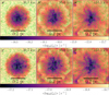 |
Fig. 2 Time evolution of the density-weighted ζ2 for models ℋ (top panels) and ℒ (bottom panels) in a sphere of 0.5 pc radius, inside which CRs are propagated. The green arrows correspond to the x-y projection of the magnetic field lines. The two different models yield a difference of one order of magnitude within the high-density region. |
3 Results
3.1 Distribution of the CR ionisation rate
Before investigating the chemical evolution in the core, we analysed the distribution of ζ2 resulting from our propagator. The code was applied to each snapshot of the simulation within a spherical region of radius 0.5 pc centred on the highest-density region of the cloud.
Figure 2 shows density-weighted maps of ζ2 for ℋ (top panels) and ℒ (bottom panels) at three different times: 30.7, 95.0, and 153.3 kyr. The x–y projection of the magnetic field lines is overplotted as green arrows. ζ2 differs by approximately one order of magnitude between the two models and spans a range of 0.6 dex. The interval below 10−16.2 s−1 (ℋ) and 10−17.1 s−1 (ℒ) covers the high-density region, as expected by considering the CR attenuation, and the highest CR ionisation rate is found in the background region where CRs are almost unattenuated. Strong twisting and bending of the magnetic field lines is also observed, especially in the highest-density regions, where the line density (hence the magnetic field intensity) also increases. This complex pattern results in a significant increase in the effective column density that is traversed by CRs, and hence, in a stronger attenuation.
The time evolution of the ζ2 distribution for the two models in a 0.2 × 0.2 × 0.2 pc3 box centred at the peak of the high-density region is shown in Fig. 3. Both distributions show that regardless of the initial ζ2 computed at injection, the attenuation reduces the initial ionisation rate by more than one order of magnitude.
In the intervals 10−16.4 to 10−15.8 s−1 (ℋ) and 10−17.3 to 10−16.7 s−1 (ℒ), the ζ2 distribution does not vary over time, but for the low- and high-end tails. In particular, the low-ζ2 tail, which is associated with the innermost region of the cloud (namely only about 1% of the total mass) simply fluctuates over time without any clear evolutionary trend. When the lowest ionisation rates per distribution, ~10−17.1 (ℋ) and ~10−18 s−1 (ℒ), are compared with Fig. F.1 of Padovani et al. (2018), these ionisation rate values correspond to column densities of ~1025–26 cm−2. In our run, this is the effect of the pitch angles that were not considered in Eq. (8), and it is related to the mirroring effect and not to a high column density accumulated by TPs.
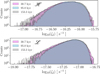 |
Fig. 3 Time evolution of the distribution of ζ2 for the gas particles in the simulation for models ℋ (top) and ℒ (bottom). The distributions are determined from a box of 0.2 × 0.2 × 0.2 pc3, which only includes particles from the simulated cloud, i.e., with identical mass. The rightmost edge of the distribution shrinks over time as the gas particles within the box become denser. The low-end tail of the distribution expands towards lower ionisation rates, which is consistent with the evolution of the gas density. |
3.2 ζ2 dependence on local properties
Because the self-consistent propagation of CRs in numerical simulations is expensive, effective models that relate the gas density to ζ2 are often employed. With our framework, we have the unique ability to determine more accurate semi-analytic prescriptions and how these prescriptions might depend on the CR model that is considered. The attenuation of ζ2 is expected to significantly depend on the gas density, under the assumption that high volume densities correspond higher column densities (Sabatini et al. 2023; Socci et al. 2024). In Fig. 4 we explore this dependence by showing the correlation between the CR ionisation rate and the number density of H2, where the viridis histogram corresponds to the ℋ model and the magma histogram to the ℒ model. The trend is clearly negative in both models, which we fit with power laws. The power law is shown as solid and dashed red lines and given by the following expressions:
![Mathematical equation: $\[\log _{10} ~\zeta_2^{\mathscr{H}}=-0.22 ~\log_{10} n(\mathrm{H}_2)-15.06,\]$](/articles/aa/full_html/2025/07/aa52470-24/aa52470-24-eq17.png) (10)
(10)
![Mathematical equation: $\[\log _{10} ~\zeta_2^{\mathscr{L}}=-0.12 ~\log _{10} n(\mathrm{H}_2)-16.45,\]$](/articles/aa/full_html/2025/07/aa52470-24/aa52470-24-eq18.png) (11)
(11)
for models ℋ and ℒ respectively. Due to the 3D structure of the system, the different lines of sight result in a slightly different CR ionisation rate, with a scatter of σℋ = 0.25 and σℒ = 0.22 for the two models (shown as shaded grey areas), calculated as the root mean square (RMS) between the actual ζ2 and our best fits.
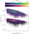 |
Fig. 4 Correlation between ζ2 and n(H2) at 153.3 kyr. The viridis and magma color maps represent the ℋ and ℒ models, respectively. The solid and dashed red lines correspond to our best-fit relations, and the shaded grey areas show the intrinsic scatter discussed in Section 3.2. |
3.3 Ion chemistry and physical correlations
We present in Fig. 5 the radial profiles obtained from column density maps of the ions HCO+, N2H+, DCO+, N2D+, and o-H2D+, together with ζ2 for the inner 0.1 pc of the simulated prestellar core. The profiles display the ℋ and ℒ models and ℒ at time 153.3 kyr. The column densities were calculated by integrating the gas cloud along a line of sight that was aligned with the z-axis over a depth of 0.2 pc. In order to exclude background gas outside the initial Bonnor-Ebert sphere representing our core, we removed gas particles with number densities below log[n/(cm−3)] < −3.78, with n calculated as ρ(2.3mp)−1 with mp the proton mass. The radial profiles were then computed by averaging the integrated quantities in circular annuli. The radial profiles (panel f) clearly show the effect of the CR attenuation in the central part (highest density). This brings the ionisation rate from model ℋ close to ζc. As a consequence, for deuterated species in particular (panels b, c, and e), the column densities of the analysed tracers approach each other. The ℒ model shows more marked differences, in particular, for deuterated species such as DCO+ and N2D+. This is due to the efficiency of the formation channels. In particular, after checking the reaction fluxes in the different cases, we found that reactions that are directly dependent on ζ2 and on (multiple) deuterated species (e.g. H2D+, D2H+, and ![Mathematical equation: $\[\mathrm{D}_{2}^{+}\]$](/articles/aa/full_html/2025/07/aa52470-24/aa52470-24-eq19.png) ) become much more relevant for high ζ2 values by boosting N2D+ and even more DCO+, as a consequence of the CO + N2D+ → N2 + DCO+ reaction. Overall, the effect of the different CR ionisation rate spectra is highly non-linear because of the attenuation effects and the different chemical evolution of these species over time.
) become much more relevant for high ζ2 values by boosting N2D+ and even more DCO+, as a consequence of the CO + N2D+ → N2 + DCO+ reaction. Overall, the effect of the different CR ionisation rate spectra is highly non-linear because of the attenuation effects and the different chemical evolution of these species over time.
We show in Fig. 6 the correlation between the abundance of electrons X(e−)and ζ2 over time for the two models with variable CR ionisation rates. The abundance was calculated from column densities obtained by integrating the gas cloud properties along the z-axis of the line of sight, as X(mol) = N(mol)/N(H2). The results for the ℋ model are shown using the outermost color map, and those for model ℒ are reported using the innermost color map. Overall, the two quantities show a clear linear correlation that remains stable over time. The distributions were fit with a power law of the form
![Mathematical equation: $\[\log_{10} ~\zeta_2^{\mathscr{H}}=0.41 ~\log _{10} X(\mathrm{e}^{-})-13.06,\]$](/articles/aa/full_html/2025/07/aa52470-24/aa52470-24-eq20.png) (12)
(12)
![Mathematical equation: $\[\log _{10} ~\zeta_2^{\mathscr{L}}=0.32 ~\log _{10} X(\mathrm{e}^{-})-14.53.\]$](/articles/aa/full_html/2025/07/aa52470-24/aa52470-24-eq21.png) (13)
(13)
At first approximation, a linear correlation is also expected for the electron abundance (or column density) and the sum of the main positive ions (DCO+, HCO+, N2H+, N2D+, and ![Mathematical equation: $\[\mathrm{H}_{3}^{+}\]$](/articles/aa/full_html/2025/07/aa52470-24/aa52470-24-eq22.png) ). Considering that
). Considering that ![Mathematical equation: $\[\mathrm{H}_{3}^{+}\]$](/articles/aa/full_html/2025/07/aa52470-24/aa52470-24-eq23.png) is not observable in the dense and cold regions of molecular clouds, we replaced it with the proxy provided by Bovino et al. (2020),
is not observable in the dense and cold regions of molecular clouds, we replaced it with the proxy provided by Bovino et al. (2020),
![Mathematical equation: $\[N\left(\mathrm{H}_3^{+}\right)_{\text {proxy }}=\frac{1}{3} \frac{N\left(\text{o-H}_2 \mathrm{D}^{+}\right)}{R_{\mathrm{D}}},\]$](/articles/aa/full_html/2025/07/aa52470-24/aa52470-24-eq24.png) (14)
(14)
where
![Mathematical equation: $\[R_{\mathrm{D}}=\frac{N(\mathrm{DCO}^{+})}{N(\mathrm{HCO}^{+})},\]$](/articles/aa/full_html/2025/07/aa52470-24/aa52470-24-eq25.png) (15)
(15)
and we tested the reliability of the following formula that can also be applied to observational data:
![Mathematical equation: $\[\begin{aligned}N(\mathrm{e}^{-})_{\text {proxy }}= & N(\mathrm{DCO}^{+})+N(\mathrm{HCO}^{+})+N(\mathrm{~N}_2 \mathrm{D}^{+}) \\& +N(\mathrm{~N}_2 \mathrm{H}^{+})+N(\mathrm{H}_3^{+})_{\text {proxy}}.\end{aligned}\]$](/articles/aa/full_html/2025/07/aa52470-24/aa52470-24-eq26.png) (16)
(16)
We show in Fig. 7 the distributions of ![Mathematical equation: $\[\mathrm{H}_{3}^{+}\]$](/articles/aa/full_html/2025/07/aa52470-24/aa52470-24-eq27.png) and e− against their proxies for models ℋ and ℒ averaged over time. The upper panel shows a very tight linear correlation between
and e− against their proxies for models ℋ and ℒ averaged over time. The upper panel shows a very tight linear correlation between ![Mathematical equation: $\[N(\mathrm{H}_{3}^{+})\]$](/articles/aa/full_html/2025/07/aa52470-24/aa52470-24-eq28.png) and
and ![Mathematical equation: $\[N\left(\mathrm{H}_{3}^{+}\right)_{\text {proxy}}\]$](/articles/aa/full_html/2025/07/aa52470-24/aa52470-24-eq29.png) up to ~1013−1014 cm−2 for both models. A deviation then appears, while the relation still remains linear, but becomes steeper. This region corresponds to the central 10 000 au, and the deviation is likely due to the neglected isotopologues in the estimation of
up to ~1013−1014 cm−2 for both models. A deviation then appears, while the relation still remains linear, but becomes steeper. This region corresponds to the central 10 000 au, and the deviation is likely due to the neglected isotopologues in the estimation of ![Mathematical equation: $\[\mathrm{H}_{3}^{+}\]$](/articles/aa/full_html/2025/07/aa52470-24/aa52470-24-eq30.png) (see Bovino et al. 2019, for a discussion). A similar behavior is also observed for the electron column density (bottom panel of Fig. 7).
(see Bovino et al. 2019, for a discussion). A similar behavior is also observed for the electron column density (bottom panel of Fig. 7).
Our proxy tends to underestimate the true electron abundance by 65% overall. This was determined as the RMS error of the ratio of the distribution of N(e−)proxy and the actual N(e−) because only a limited number of ions was included in the formula and the approximations made. The analytical formula reported in Eq. (16) was validated by employing a simulation of a typical prestellar core, specifically, on sub-parsec scales, but it also holds on larger scales and has a wider and more general applicability within the approximation we introduced so far. First, in the sum we neglected the contribution of ions that might become important (e.g. H3O+ among others) and the charged grains that might be relevant in star-forming regions, which particularly affects the total negative charge. In addition, when we probed ![Mathematical equation: $\[\mathrm{H}_{3}^{+}\]$](/articles/aa/full_html/2025/07/aa52470-24/aa52470-24-eq33.png) through its first deuterated product (H2D+), we neglected other isotopologues that become important when the core central densities increase (see also Bovino et al. 2020; Redaelli et al. 2024). Finally, we worked with averaged quantities (column densities) to estimate local physical variables. For these reasons, the estimates of the ionisation fraction we provide represent a robust (within a factor of two) lower limit of the real value.
through its first deuterated product (H2D+), we neglected other isotopologues that become important when the core central densities increase (see also Bovino et al. 2020; Redaelli et al. 2024). Finally, we worked with averaged quantities (column densities) to estimate local physical variables. For these reasons, the estimates of the ionisation fraction we provide represent a robust (within a factor of two) lower limit of the real value.
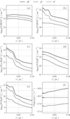 |
Fig. 5 Radial profiles of the column densities of HCO+(a), DCO+ (b), o-H2D+(c), N2H+(d), and N2D+(e) ions and the ζ2 distribution (f) at 153.3 kyr. The ζ2 radial profile is calculated in circular annuli from the average along the line of sight (as shown in Fig. 2). The CR ionisation models ℋ, ℒ, and ℒ are represented by solid, dashed, and dotted black lines, respectively. |
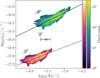 |
Fig. 6 Correlation between X(e−)and ζ2 obtained from the 2D maps (line-of-sight averages) for models ℋ (outermost color scale) and ℒ (innermost color scale), combining different time snapshots (t = 30.7, 95.0, and 153.3 kyr). The solid and dashed lines correspond to power-law fits. The cross located at log10(ζc) = −16.6 represents the median of the electron abundance (X(e−)) for the ℒ model, and the error bars are the 1σ of the data. |
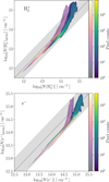 |
Fig. 7 Pixel-by-pixel 2D histogram distributions for the ℋ (viridis) and ℒ (magma) model by combining different times (t = 30.7, 95.0, and 153.3 kyr). The upper panel correlates the |
![Mathematical equation: $\[\mathrm{H}_{3}^{+}\]$](/articles/aa/full_html/2025/07/aa52470-24/aa52470-24-eq31.png)
![Mathematical equation: $\[\mathrm{H}_{3}^{+}\]$](/articles/aa/full_html/2025/07/aa52470-24/aa52470-24-eq32.png)
3.4 Ionisation fraction in observed clumps
To show an application of the analytical formula presented in Eq. (16), we employed recent available data for five high-mass clumps at different evolutionary stages: namely G13.18+0.06, G14.11-0.57, G14.63-0.58, G15.72-0.59, and G19.88-0.54. These sources were selected from the APEX3 Telescope Large Area Survey of the Galaxy (ATLASGAL; Schuller et al. 2009), where they have reliable estimates of kinematic distances, masses, luminosities, and dust temperatures (e.g. Urquhart et al. 2022), employed in this derivation.
We used the data presented by Sabatini et al. (2020, 2024) for all tracers in Eq. (16). Sabatini et al. (2020) observed o-H2D+ (110−111), N2H+ (4–3), DCO+ (1–0), and H13CO+ (1–0) with the APEX and IRAM-30m telescopes. Additional N2D+(3–2) data were obtained with the nFLASH receiver mounted at APEX through two projects (project-IDs: C-0105.F-9715C-2020 and C-0107.F-9711-2021; PIs: S. Bovino and G. Sabatini, respectively). We refer to Sabatini et al. (2020, 2024) for a full description of the observations and the data analysis.
Considering the recent updates of dust temperatures for ATLASGAL clumps (Urquhart et al. 2022), and following Sabatini et al. (2020), we derived the column densities using MCWeeds (Giannetti et al. 2017), which is an interface between Weeds (Maret et al. 2011) and the Bayesian statistical models of PyMC (Patil et al. 2010), and we assumed Tex = Tdust equal to 20.3 K (G13.18+0.06), 15.8 K (G14.11-0.57), 19.1 K (G14.63-0.58), 12.1 K (G15.72-0.59), and 20.3 K (G19.88-0.54). The final column densities are in the range ~(0.8–3.2) × 1012 cm−2 for o-H2D+, ~(3.7–5.9) × 1011 cm−2 for N2D+, ~(0.2–3.0) × 1013 cm−2 for N2H+, ~(0.6–4.0) × 1013 cm−2 for DCO+, and ~(1.6–6.3) × 1013 cm−2 for H13CO+. This matches the typical abundances relative to H2 in high-mass star-forming clumps (e.g. Miettinen 2020; Sabatini et al. 2020; Li et al. 2022). The average error on the computed column densities is ≲20%. We calculated N(HCO+) from N(H13CO+) taking into account a 12C/13C ratio that changes as a function of the galactocentric distance (DGC) of each source; that is, [12C]/13C] = ![Mathematical equation: $\[6.1_{-1.8}^{+1.1}\]$](/articles/aa/full_html/2025/07/aa52470-24/aa52470-24-eq34.png) DGC +
DGC + ![Mathematical equation: $\[14.3_{-7.2}^{+7.7}\]$](/articles/aa/full_html/2025/07/aa52470-24/aa52470-24-eq35.png) (Giannetti et al. 2014). When applying Eq. (16) to this range of column densities, we obtained N(e−)in the range ~(1.1–3.9) ± 0.5 × 1015 cm−2, corresponding to X(e−)from 1.8 × 10⁻⁸ to 2.7 × 10⁻⁸. We note that a typical uncertainty of ~30% is associated with X(e−), which results from propagating the uncertainty on the integrated line intensity.
(Giannetti et al. 2014). When applying Eq. (16) to this range of column densities, we obtained N(e−)in the range ~(1.1–3.9) ± 0.5 × 1015 cm−2, corresponding to X(e−)from 1.8 × 10⁻⁸ to 2.7 × 10⁻⁸. We note that a typical uncertainty of ~30% is associated with X(e−), which results from propagating the uncertainty on the integrated line intensity.
Regardless of the scale difference between observations (~1 pc) and simulation (~0.1 pc), HCO+ is the dominating ion in both cases, together with ![Mathematical equation: $\[\mathrm{H}_{3}^{+}\]$](/articles/aa/full_html/2025/07/aa52470-24/aa52470-24-eq36.png) (and its isotopologues) that is necessary to recover the electron abundance in the central region. This confirms the reliability of the method even when it is applied on different scales. The simulations and observations we analysed clearly represent specific physical cases. We expect the formula to work also in situations in which other ions dominate the overall sum, in particular, cases in which small scales are properly resolved by high-resolution observations (e.g. using the Atacama Large Millimeter Array; ALMA) that might unveil emission and a contribution from more compact tracers.
(and its isotopologues) that is necessary to recover the electron abundance in the central region. This confirms the reliability of the method even when it is applied on different scales. The simulations and observations we analysed clearly represent specific physical cases. We expect the formula to work also in situations in which other ions dominate the overall sum, in particular, cases in which small scales are properly resolved by high-resolution observations (e.g. using the Atacama Large Millimeter Array; ALMA) that might unveil emission and a contribution from more compact tracers.
4 Conclusions
We have introduced a CR propagation code for accurately estimating the CR ionisation rate in MHD simulations. We coupled our code to the outputs of MHD simulations performed with GIZMO by implementing an interpolation scheme of gas properties consistent with the smoothing kernel procedure in the simulation. The propagator maps CRs as a flux of TPs for which the effective column density that is traversed following the magnetic field lines is determined by means of a Runge-Kutta integrator. The CR ionisation rate at the location of each TP was then estimated according to the ℋ and ℒ models by Padovani et al. (2018) and was deposited onto the gas tracers in the original simulation in a self-consistent way. The results of the propagator were then used to investigate the evolution of several ions whose abundances are directly affected by CRs.
We tested the convergence of the code and found the optimal number of TPs (see Appendix A) that balance accuracy and performance (10 240). We therefore demonstrated that this number is adequate enough to generate a reliable characterisation of the CR ionisation rate of the object because the differences from the most expensive run (32 times more TPs) are minimal and mostly affect the background region.
After the optimal number of TPs was found, we analysed the time evolution of the chemistry in a collapsing magnetised prestellar core from Bovino et al. (2019) by employing the KROME framework in post-processing as described by Ferrada-Chamorro et al. (2021). We focussed on three different CR models, two variable cases (ℋ and ℒ in Padovani et al. 2018) evolved by means of the propagation scheme, and a reference constant case with ζ2 = 2.5 × 10⁻¹⁷ s−1, with the aim to assess the CR propagation impact on the chemistry.
We found that a proper CR propagation scheme can produce significant differences (with a non-linear behaviour) for key chemical tracers, in particular, on deuterated species such as DCO+ and N2D+. We also analysed the correlations between the electron abundance X(e−)and ζ2 and between the electron column density and the column density of the most relevant positive ions. We found that clear correlations exist in both cases, and the two CR ionisation models ℋ and ℒ only yield a different normalisation. In particular, we provided an analytical function to estimate the electron abundance in star-forming regions with a standard deviation of 0.6, and we showed that when applied to observational data, it provides reliable estimates. For early stages high-mass clumps, we reported values around 10−8 that agree with previous estimates of prestellar regions (e.g. Caselli et al. 1998; Bergin et al. 1999; Maret & Bergin 2007). We analysed the correlation between ζ2 and n(H2) and determined the best-fit expressions, with an uncertainty of ~25% that could be employed as an approximate estimator for ζ2 in numerical simulations without a self-consistent CR propagation scheme.
Finally, the increasing capabilities of modern astronomical facilities such as ALMA represent a viable method for testing our predictions. Additional high-sensitivity and high-resolution observations of the molecular tracers involved in Eq. (16) are needed to reveal possible fluctuations in electron abundance on core scales. In this context, intensive observational campaigns such as the recently accepted ALMA large program UNveiling the Initial Conditions of high-mass star-formation (UNIC)4, which targets ten massive clumps with potentially more than 130 embedded cores, offer a unique opportunity to extend the results reported in this work under a variety of physical and chemical conditions in the near future.
Acknowledgements
GL gratefully acknowledges the financial support of ANID-Subdirección de Capital Humano/Magíster Nacional/2024-22241873 and Millenium Nucleus NCN23_002 (TITANs). SB acknowledges BASAL Centro de Astrofisica y Tecnologias Afines (CATA), project number AFB-17002. GS acknowledges the PRIN-MUR 2020 BEYOND-2p (Astrochemistry beyond the Second period elements, Prot. 2020AFB3FX), the project ASI-Astrobiologia 2023 MIGLIORA (Modeling Chemical Complexity, F83C23000800005), the INAF Mini-grant 2023 TRIESTE (“TRacing the chemIcal hEritage of our originS: from proTostars to planEts”; PI: G. Sabatini), and the National Recovery and Resilience Plan (NRRP), Mission 4, Component 2, Investment 1.1, Call for tender No. 104 published on 2.2.2022 by the Italian Ministry of University and Research (MUR), funded by the European Union – NextGenerationEU-Project Title 2022JC2Y93 Chemical Origins: linking the fossil composition of the Solar System with the chemistry of protoplanetary disks – CUP J53D23001600006 – Grant Assignment Decree No. 962 adopted on 30.06.2023 by the Italian Ministry of MUR.
Appendix A Convergence tests
Because of our choice of kernel size, the scheme does not guarantee that all gas particles in the original simulation are used for the calculation. When this happens, ζ2 is set to zero, which would yield an inaccurate chemical evolution. In order to avoid this issue, there are two possible solutions. The computationally cheapest one, that however we have not considered in this work, is similar in spirit to the approach in Ferrada-Chamorro et al. (2021), and interpolates ζ2 using the values of the neighbouring gas particles. The other possibility, that we have employed here, as it guarantees a much higher accuracy, requires a sufficiently large number of TPs, so that no regions of the cloud are left uncovered during the TP propagation.
In order to identify the minimum number of particles required to reach convergence, that is our ‘fiducial’ case, we explored different values of TPs in a suite of test runs, starting from 5120 TPs and gradually increasing their number by a factor of two, as reported in Table A.1.
Number of TPs in the suite of convergence runs performed. The fiducial case is highlighted in boldface.
In Fig. A.1, we show the distribution of ζ2 per particle for the ℋ case (left-hand panels), and for the ℒ case (right-hand panel), comparing each run in Table A.1 with our fiducial case (X2). Most of the particles are located on the rightmost side of the distribution, with a long tail extending to low ζ2 values. This reflects that gas particles with large ζ2 are located near the edge of the cloud where the attenuation is not strong yet, before the steep decrease begins as we move towards the centre of the cloud, which corresponds to the leftmost tail where the attenuation is the strongest. In general, we find a reasonable agreement in the shape of the distribution among the runs, which is consistent with the fact that the distribution is mainly determined by the physical properties of the cloud, which does not vary. The only differences we find can thus be attributed to the number of TPs used, which affects the smoothing procedure and the integration step. On one hand, X1 exhibits an overestimation at the edges of the distribution, because of the poor spatial sampling that is more sensitive to outliers. On the other hand, the increase of TPs slowly carves the high-ζ2 region, thanks to a better spatial sampling which removes the outliers, but does not significantly change the low-ζ2 tail, which instead shows stochastic variations due to the small number of gas particles in the central region. This comparison implies that the X2 case represents the best compromise between accuracy and efficiency for the chemical analysis we are interested in. For sake of completeness, in Appendix B we analyse the relative error in the line-of-sight projection of ζ2 between our fiducial run and the other five runs.
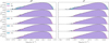 |
Fig. A.1 ζ2 distribution for ℋ (left) and ℒ (right) at 153.3 kyr in a 0.2 × 0.2 × 0.2 pc3 box. In each row, we compared one of the runs in Table A.1 (in cyan) with our fiducial case (X2, in pink), with the matching regions in purple. fpart represents the fraction of particles. |
Appendix B Relative error of expensive runs
Fig. B.1 shows the relative difference between ζ2 obtained in our fiducial case, X2, and the other runs employing different numbers of TPs, averaged along a line-of-sight aligned with the z-axis. The largest and smallest relative error among the pixels are reported in the bottom left corner of every panel, corresponding to X1, X4, X8, X16, and X32 from top to bottom, respectively. We clearly observe larger deviations for the X1 case, whereas the other cases oscillate around 10–20% almost independently of resolution.
To further check the robustness of our calculations, we determined the error within a spherical region of radius 0.065 pc (identified by the green dashed circle), comparable to the typical size of star-forming filaments. The relative error in this case drops by about a factor of 2, reaching at most 3–13% for both ionisation models. The use of 10240 particles (our base) seems therefore adequate, as higher resolution runs do not significantly improve the results, but at the same time require a much higher computational cost. Obviously, on the largest scales explored here, the errors are larger, but this is expected as we start to encompass more background gas as well, which has lower column densities, hence is more easily affected by variations in ζ2.
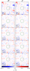 |
Fig. B.1 Relative error (ϵ) for ℋ (left) and ℒ (right) within a 0.5 × 0.5 × 0.2 pc3 at 153.3 kyr. We chose this box size to take into account the 0.5 pc of injection and a depth length similar to the filament scale (0.2 pc) to avoid the inclusion of background particles. The errors are calculated between X2 case and the rest. The panels are, from top to bottom: X1, X4, X8, X16 and X32. The bluer and redder indicate underestimation and overestimation of X2 relative to the others. The maximum and minimum errors for each comparison are written in the bottom-left corner. All green spheres have 0.065 pc radii. |
References
- Bergin, E. A., & Tafalla, M. 2007, ARA&A, 45, 339 [Google Scholar]
- Bergin, E. A., Plume, R., Williams, J. P., & Myers, P. C. 1999, ApJ, 512, 724 [NASA ADS] [CrossRef] [Google Scholar]
- Bialy, S., Belli, S., & Padovani, M. 2022, A&A, 658, L13 [NASA ADS] [CrossRef] [EDP Sciences] [Google Scholar]
- Bovino, S., Ferrada-Chamorro, S., Lupi, A., et al. 2019, ApJ, 887, 224 [NASA ADS] [CrossRef] [Google Scholar]
- Bovino, S., Ferrada-Chamorro, S., Lupi, A., Schleicher, D. R. G., & Caselli, P. 2020, MNRAS, 495, L7 [Google Scholar]
- Bustard, C., & Zweibel, E. G. 2021, ApJ, 913, 106 [NASA ADS] [CrossRef] [Google Scholar]
- Caselli, P., Walmsley, C. M., Terzieva, R., & Herbst, E. 1998, ApJ, 499, 234 [Google Scholar]
- Caselli, P., Sipilä, O., & Harju, J. 2019, Philos. Trans. Roy. Soc. A: Math. Phys. Eng. Sci., 377, 20180401 [Google Scholar]
- Ceccarelli, C., Dominik, C., López-Sepulcre, A., et al. 2014, ApJ, 790, L1 [Google Scholar]
- Chan, T. K., Kereš, D., Hopkins, P. F., et al. 2019, MNRAS, 488, 3716 [NASA ADS] [CrossRef] [Google Scholar]
- Dalgarno, A. 2006, Proc. Natl. Acad. Sci., 103, 12269 [NASA ADS] [CrossRef] [Google Scholar]
- Dalgarno, A., & Lepp, S. 1984, ApJ, 287, L47 [NASA ADS] [CrossRef] [Google Scholar]
- Ferrada-Chamorro, S., Lupi, A., & Bovino, S. 2021, MNRAS, 505, 3442 [NASA ADS] [CrossRef] [Google Scholar]
- Gaches, B. A. L., Bisbas, T. G., & Bialy, S. 2022, A&A, 658, A151 [CrossRef] [EDP Sciences] [Google Scholar]
- Giannetti, A., Wyrowski, F., Brand, J., et al. 2014, A&A, 570, A65 [NASA ADS] [CrossRef] [EDP Sciences] [Google Scholar]
- Giannetti, A., Leurini, S., Wyrowski, F., et al. 2017, A&A, 603, A33 [NASA ADS] [CrossRef] [EDP Sciences] [Google Scholar]
- Grassi, T., Bovino, S., Schleicher, D. R. G., et al. 2014, MNRAS, 439, 2386 [Google Scholar]
- Güsten, R., Nyman, L. A., Schilke, P., et al. 2006, A&A, 454, L13 [NASA ADS] [CrossRef] [EDP Sciences] [Google Scholar]
- Hopkins, P. F. 2015, MNRAS, 450, 53 [Google Scholar]
- Hopkins, P. F., & Raives, M. J. 2016, MNRAS, 455, 51 [NASA ADS] [CrossRef] [Google Scholar]
- Indriolo, N., & McCall, B. J. 2012, ApJ, 745, 91 [NASA ADS] [CrossRef] [Google Scholar]
- Indriolo, N., & McCall, B. J. 2013, Chem. Soc. Rev., 42, 7763 [NASA ADS] [CrossRef] [Google Scholar]
- Indriolo, N., Geballe, T. R., Oka, T., & McCall, B. J. 2007, ApJ, 671, 1736 [NASA ADS] [CrossRef] [Google Scholar]
- Indriolo, N., Neufeld, D. A., Gerin, M., et al. 2012, ApJ, 758, 83 [NASA ADS] [CrossRef] [Google Scholar]
- Li, S., Sanhueza, P., Lu, X., et al. 2022, ApJ, 939, 102 [CrossRef] [Google Scholar]
- Maret, S., & Bergin, E. A. 2007, ApJ, 664, 956 [Google Scholar]
- Maret, S., Hily-Blant, P., Pety, J., Bardeau, S., & Reynier, E. 2011, A&A, 526, A47 [NASA ADS] [CrossRef] [EDP Sciences] [Google Scholar]
- Miettinen, O. 2020, A&A, 634, A115 [NASA ADS] [CrossRef] [EDP Sciences] [Google Scholar]
- Neufeld, D. A., & Wolfire, M. G. 2017, ApJ, 845, 163 [Google Scholar]
- Obolentseva, M., Ivlev, A. V., Silsbee, K., et al. 2024, ApJ, 973, 142 [NASA ADS] [CrossRef] [Google Scholar]
- Ogrodnik, M. A., Hanasz, M., & Wóltański, D. 2021, ApJS, 253, 18 [CrossRef] [Google Scholar]
- Padovani, M., & Gaches, B. 2024, in Astrochemical Modeling: Practical Aspects of Microphysics in Numerical Simulations, ed. S. Bovino, & T. Grassi (Elsevier), 189 [Google Scholar]
- Padovani, M., Hennebelle, P., & Galli, D. 2013, A&A, 560, A114 [NASA ADS] [CrossRef] [EDP Sciences] [Google Scholar]
- Padovani, M., Ivlev, A. V., Galli, D., & Caselli, P. 2018, A&A, 614, A111 [NASA ADS] [CrossRef] [EDP Sciences] [Google Scholar]
- Padovani, M., Ivlev, A. V., Galli, D., et al. 2020, Space Sci. Rev., 216, 29 [CrossRef] [Google Scholar]
- Padovani, M., Bialy, S., Galli, D., et al. 2022, A&A, 658, A189 [NASA ADS] [CrossRef] [EDP Sciences] [Google Scholar]
- Patil, A., Huard, D., & Fonnesbeck, C. J. 2010, J. Statist. Softw., 35, 1 [Google Scholar]
- Redaelli, E., Sipilä, O., Padovani, M., et al. 2021, A&A, 656, A109 [NASA ADS] [CrossRef] [EDP Sciences] [Google Scholar]
- Redaelli, E., Bovino, S., Lupi, A., et al. 2024, A&A, 685, A67 [NASA ADS] [CrossRef] [EDP Sciences] [Google Scholar]
- Sabatini, G., Bovino, S., Giannetti, A., et al. 2020, A&A, 644, A34 [EDP Sciences] [Google Scholar]
- Sabatini, G., Bovino, S., & Redaelli, E. 2023, ApJ, 947, L18 [NASA ADS] [CrossRef] [Google Scholar]
- Sabatini, G., Bovino, S., Redaelli, E., et al. 2024, A&A, 692, A265 [NASA ADS] [CrossRef] [EDP Sciences] [Google Scholar]
- Schuller, F., Menten, K. M., Contreras, Y., et al. 2009, A&A, 504, 415 [NASA ADS] [CrossRef] [EDP Sciences] [Google Scholar]
- Shaw, G., Ferland, G. J., Srianand, R., et al. 2008, ApJ, 675, 405 [NASA ADS] [CrossRef] [Google Scholar]
- Shingledecker, C. N., Bergner, J. B., Le Gal, R., et al. 2016, ApJ, 830, 151 [NASA ADS] [CrossRef] [Google Scholar]
- Silsbee, K., Ivlev, A. V., Padovani, M., & Caselli, P. 2018, ApJ, 863, 188 [Google Scholar]
- Snow, T. P., & McCall, B. J. 2006, ARA&A, 44, 367 [NASA ADS] [CrossRef] [Google Scholar]
- Socci, A., Sabatini, G., Padovani, M., Bovino, S., & Hacar, A. 2024, A&A, 687, A70 [NASA ADS] [CrossRef] [EDP Sciences] [Google Scholar]
- Springel, V. 2005, MNRAS, 364, 1105 [Google Scholar]
- Thomas, T., Pfrommer, C., & Pakmor, R. 2021, MNRAS, 503, 2242 [Google Scholar]
- Urquhart, J. S., Wells, M. R. A., Pillai, T., et al. 2022, MNRAS, 510, 3389 [NASA ADS] [CrossRef] [Google Scholar]
- Winner, G., Pfrommer, C., Girichidis, P., & Pakmor, R. 2019, MNRAS, 488, 2235 [Google Scholar]
We verified that convergence was typically reached in up to three iterations.
Note that recently the estimates of ζ2 for diffuse clouds have been revised in Obolentseva et al. (2024). This model would then represent an upper limit to diffuse clouds estimates.
Atacama Pathfinder EXperiment 12 meter submillimeter telescope (APEX; Güsten et al. 2006). APEX has been a collaboration between the Max Planck Institute for Radioastronomy, the European Southern Observatory, and the Onsala Space Observatory.
All Tables
Number of TPs in the suite of convergence runs performed. The fiducial case is highlighted in boldface.
All Figures
|
Fig. 1 Sketch of the CR propagation scheme based on the structure given in Section 2.1. The left panel describes the TP propagation through the domain. TPs (grey dots) are created from a spherical surface of radius R (dashed black circle) with radial inward trajectories (step i). TPs are then deactivated when the column density that is traversed exceeds 1029 cm−2 or when they leave the outer spherical surface at a distance Rout (solid black circle), as shown by the crossed grey dots. The right panel instead highlights the propagation of a single TP particle. The trajectory is shown by the curved solid blue arrow, and the magnetic field lines (B) are reported as dash-dotted grey lines. The pitch angle (α) between the TP velocity and the local magnetic field is shown as the dashed red line. The displacement of the TP between the previous (x) and the current (x′) location is defined by the step size Δℓ (step iii). To compute the effective column density of the TP, the average local density (n(x′)) and local magnetic field (B(x′)) were estimated from gas particles (pink dots) within the kernel size h (thin yellow arrows; step ii). Then, its value was used to update the CR ionisation rate (ζ2; step iv), which was finally deposited at the location of the original gas particle (thick yellow arrows; step v). |
| In the text | |
|
Fig. 2 Time evolution of the density-weighted ζ2 for models ℋ (top panels) and ℒ (bottom panels) in a sphere of 0.5 pc radius, inside which CRs are propagated. The green arrows correspond to the x-y projection of the magnetic field lines. The two different models yield a difference of one order of magnitude within the high-density region. |
| In the text | |
|
Fig. 3 Time evolution of the distribution of ζ2 for the gas particles in the simulation for models ℋ (top) and ℒ (bottom). The distributions are determined from a box of 0.2 × 0.2 × 0.2 pc3, which only includes particles from the simulated cloud, i.e., with identical mass. The rightmost edge of the distribution shrinks over time as the gas particles within the box become denser. The low-end tail of the distribution expands towards lower ionisation rates, which is consistent with the evolution of the gas density. |
| In the text | |
|
Fig. 4 Correlation between ζ2 and n(H2) at 153.3 kyr. The viridis and magma color maps represent the ℋ and ℒ models, respectively. The solid and dashed red lines correspond to our best-fit relations, and the shaded grey areas show the intrinsic scatter discussed in Section 3.2. |
| In the text | |
|
Fig. 5 Radial profiles of the column densities of HCO+(a), DCO+ (b), o-H2D+(c), N2H+(d), and N2D+(e) ions and the ζ2 distribution (f) at 153.3 kyr. The ζ2 radial profile is calculated in circular annuli from the average along the line of sight (as shown in Fig. 2). The CR ionisation models ℋ, ℒ, and ℒ are represented by solid, dashed, and dotted black lines, respectively. |
| In the text | |
|
Fig. 6 Correlation between X(e−)and ζ2 obtained from the 2D maps (line-of-sight averages) for models ℋ (outermost color scale) and ℒ (innermost color scale), combining different time snapshots (t = 30.7, 95.0, and 153.3 kyr). The solid and dashed lines correspond to power-law fits. The cross located at log10(ζc) = −16.6 represents the median of the electron abundance (X(e−)) for the ℒ model, and the error bars are the 1σ of the data. |
| In the text | |
|
Fig. 7 Pixel-by-pixel 2D histogram distributions for the ℋ (viridis) and ℒ (magma) model by combining different times (t = 30.7, 95.0, and 153.3 kyr). The upper panel correlates the |
| In the text | |
|
Fig. A.1 ζ2 distribution for ℋ (left) and ℒ (right) at 153.3 kyr in a 0.2 × 0.2 × 0.2 pc3 box. In each row, we compared one of the runs in Table A.1 (in cyan) with our fiducial case (X2, in pink), with the matching regions in purple. fpart represents the fraction of particles. |
| In the text | |
|
Fig. B.1 Relative error (ϵ) for ℋ (left) and ℒ (right) within a 0.5 × 0.5 × 0.2 pc3 at 153.3 kyr. We chose this box size to take into account the 0.5 pc of injection and a depth length similar to the filament scale (0.2 pc) to avoid the inclusion of background particles. The errors are calculated between X2 case and the rest. The panels are, from top to bottom: X1, X4, X8, X16 and X32. The bluer and redder indicate underestimation and overestimation of X2 relative to the others. The maximum and minimum errors for each comparison are written in the bottom-left corner. All green spheres have 0.065 pc radii. |
| In the text | |
Current usage metrics show cumulative count of Article Views (full-text article views including HTML views, PDF and ePub downloads, according to the available data) and Abstracts Views on Vision4Press platform.
Data correspond to usage on the plateform after 2015. The current usage metrics is available 48-96 hours after online publication and is updated daily on week days.
Initial download of the metrics may take a while.