| Issue |
A&A
Volume 649, May 2021
|
|
|---|---|---|
| Article Number | A95 | |
| Number of page(s) | 19 | |
| Section | Interstellar and circumstellar matter | |
| DOI | https://doi.org/10.1051/0004-6361/202039200 | |
| Published online | 19 May 2021 | |
CO isotopolog line fluxes of viscously evolving disks
Cold CO conversion insufficient to explain observed low fluxes
1
Leiden Observatory, Leiden University,
Niels Bohrweg 2,
2333
CA
Leiden, The Netherlands
2
Department of Astronomy, University of Wisconsin-Madison,
475 N Charter St,
Madison,
WI,
53706, USA
e-mail: ltrapman@wisc.edu
3
Department of Astronomy, University of Michigan, 1085 S. University Ave,
Ann Arbor,
MI
48109, USA
4
School of Physics and Astronomy, University of Leicester,
Leicester
LE1 7RH, UK
5
Anton Pannekoek Institute for Astronomy, University of Amsterdam,
Science Park 904,
1090 GE
Amsterdam, The Netherlands
6
Max-Planck-institute für Extraterrestrische Physik,
Giessenbachstraße,
85748
Garching, Germany
Received:
17
August
2020
Accepted:
3
March
2021
Context. Protoplanetary disks are thought to evolve viscously, where the disk mass – the reservoir available for planet formation – decreases over time as material is accreted onto the central star over a viscous timescale. Observations have shown a correlation between disk mass and the stellar mass accretion rate, as expected from viscous theory. However, this happens only when using the dust mass as a proxy of the disk mass; the gas mass inferred from CO isotopolog line fluxes, which should be a more direct measurement, shows no correlation with the stellar mass accretion rate.
Aims. We investigate how 13CO and C18O J = 3−2 line fluxes, commonly used as gas mass tracers, change over time in a viscously evolving disk and use them together with gas disk sizes to provide diagnostics of viscous evolution. In addition, we aim to determine if the chemical conversion of CO through grain-surface chemistry combined with viscous evolution can explain the CO isotopolog observations of disks in Lupus.
Methods. We ran a series of thermochemical DALI models of viscously evolving disks, where the initial disk mass is derived from observed stellar mass accretion rates.
Results. While the disk mass, Mdisk, decreases over time, the 13CO and C18O J = 3−2 line fluxes instead increase over time due to their optically thick emitting regions growing in size as the disk expands viscously. The C18O 3–2 emission is optically thin throughout the disk for only for a subset of our models (M*≤ 0.2 M⊙ and αvisc ≥ 10−3, corresponding to Mdisk(t = 1 Myr) ≤ 10−3 M⊙). For these disks the integrated C18O flux decreases with time, similar to the disk mass. Observed 13CO and C18O 3–2 fluxes of the most massive disks (Mdisk ≳ 5 × 10⁻³ M⊙) in Lupus can be reproduced to within a factor of ~2 with viscously evolving disks in which CO is converted into other species through grain-surface chemistry with a moderate cosmic-ray ionization rate of ζcr ~ 10−17 s−1. The C18O 3–2 fluxes for the bulk of the disks in Lupus (with Mdisk ≲ 5 × 10⁻³ M⊙) can be reproduced to within a factor of ~2 by increasing ζcr to ~ 5 × 10⁻¹⁷−10−16 s−1, although explaining the stacked upper limits requires a lower average abundance than our models can produce. In addition, increasing ζcr cannot explain the observed 13CO fluxes for lower mass disks, which are more than an order of magnitude fainter than what is predicted. In our models the optically thick 13CO emission originates from a layer higher up in the disk (z∕r ~ 0.25−0.4) where photodissociation stops the conversion of CO into other species. Reconciling the 13CO fluxes of viscously evolving disks with the observations requires either efficient vertical mixing or low mass disks (Mdust ≲ 3 × 10⁻⁵ M⊙) being much thinner and/or smaller than their more massive counterparts.
Conclusions. The 13CO model flux predominantly traces the disk size, but the C18O model flux traces the disk mass of our viscously evolving disk models if chemical conversion of CO is included. The discrepancy between the CO isotopolog line fluxes of viscously evolving disk models and the observations suggests that CO is efficiently vertically mixed or that low mass disks are smaller and/or colder than previously assumed.
Key words: protoplanetary disks / astrochemistry / radiative transfer / line: formation
© ESO 2021
1 Introduction
With over 4200 exoplanets detected1 in a multitude of planetary systems, it has become clear that the formation of planets around young stars is a common occurrence (see, e.g., Borucki et al. 2011; Winn & Fabrycky 2015; Morton et al. 2016). Understanding the processes behind the formation of planets has proven challenging. A key ingredient is the total amount of material available in the protoplanetary disks in which these planets form and grow (see, e.g., Benz et al. 2014; Armitage 2015; Mordasini 2018). The disk mass determines how much raw material can be accreted onto the forming planets. The disk mass is also not static as accretion onto the central star slowly decreases its mass over time. Combined, the disk mass and the stellar mass accretion rate determine the lifetime of the disk and therefore set an upper limit to the duration of planet formation. Determining disk masses and how they evolve over time is therefore crucial for our understanding of planet formation.
It is commonly assumed that protoplanetary disks evolve viscously (see, e.g., Lynden-Bell & Pringle 1974; Shakura & Sunyaev 1973). Viscous stresses in the disk transport angular momentum outward, causing the outer parts of the disk to spread out. To conserve angular momentum, this causes material to be transported inward, where it is accreted onto the central star.While still debated, the physical process behind this effective viscosity is commonly assumed to be the magnetorotational instability (see, e.g., Balbus & Hawley 1991, 1998). In the framework of viscous evolution, the disk mass, Mdisk, and the stellar mass accretion rate, Ṁacc, follow a linear relation, with the disk mass being accreted onto the star on a viscous timescale (Mdisk ~Ṁacctvisc).
Alternatively, it has been suggested that the angular momentum in disks can be removed by a magnetic disk wind rather than transported outward by viscous stresses (see, e.g. Turner et al. 2014). This magnetic disk wind forms in the presence of a vertical magnetic field in the disk, and it is able to remove material from the disk surface, thus reducing the total angular momentum in the disk. What fraction of the angular momentum can be carried away by the disk wind is still a matter of debate (see, e.g., Ferreira et al. 2006; Béthune et al. 2017; Zhu & Stone 2018). Magnetic disk winds have been detected in observations but predominantly in the inner part of the disk, and it remains unclear how much disk winds affect disk evolution (see, e.g., Pontoppidan et al. 2011; Bjerkeli et al. 2016; Tabone et al. 2017; de Valon et al. 2020).
Recently, several combined observing campaigns have performed large surveys of the full disk population, allowing the simultaneous study of properties of protoplanetary disks and the young stellar objects that host them. Several star-forming regions havebeen covered by Atacama Large Millimeter/submillimeter Array (ALMA) disk surveys, providing high angular resolution observations of disk continuum emission and carbon monoxide (CO) rotational line emission (e.g., Ansdell et al. 2016, 2017, 2018; Barenfeld et al. 2016, 2017; Pascucci et al. 2016; Long et al. 2017; Cazzoletti et al. 2019; Cox et al. 2017; Cieza et al. 2019; Williams et al. 2019). Using spectra from the X-shooter spectrograph (Vernet et al. 2011) at the ESO Very Large Telescope, stellar properties such as the stellar mass accretion rate have also been measured for a large fraction of the disk-hosting stars in star-forming regions such as Lupus, Chamaeleon I, and Upper Sco (Alcalá et al. 2014, 2017; Manara et al. 2017, 2020).
Combining observations for the disk population in Lupus, Manara et al. (2016) found a correlation between the observed stellar mass accretion rate, Ṁacc, and the disk dust mass, Mdust, derived from millimeter continuum emission. If an interstellar medium (ISM) gas-to-dust mass ratio Δgd = 100 is assumed, the observations (Ṁacc and Mdisk = 100 × Mdust) are consistent with viscous disks having evolved for 1–3 Myr, which matches the approximate age of the sources (see also Rosotti et al. 2017). Interestingly, they find no correlation between Ṁacc and the disk gas mass, Mgas, derived from 13CO J = 3−2 and C18O J = 3−2 line fluxes. This seems to contradict their first finding, suggesting that the disk gas mass, which is expected to make up most of the total disk mass, is not related to the stellar mass accretion rate.
The cause for this discrepancy might lie with the tracer used to measure the disk gas mass. For most disks the gas masses derived from optically thin CO isotopologs such as 13CO and C18O are found to be low compared to their dust mass, with Δgd = Mgas∕Mdust ≈ 1−10 for most disks (see, e.g., Ansdell et al. 2016; Miotello et al. 2017; Long et al. 2017). Herschel Space observatory observations of the hydrogen deuteride (HD) J = 1−0 rotational line toward a handful of disks have provided an independent measurement of the disk gas mass (Bergin et al. 2013; McClure et al. 2016; Trapman et al. 2017; Kama et al. 2020). These observations find a gas-to-dust mass ratio of ~ 100, suggesting that the low CO-based gas masses are a sign that disks are underabundant in CO. This underabundance is in addition to well-understood processes such as CO freeze-out and photodissociation. Several processes have been suggested to explain the extra underabundance of CO, such as chemical conversion of CO in the gas or on the grains into more complex species (e.g., Aikawa et al. 1997; Bergin et al. 2014; Furuya & Aikawa 2014; Yu et al. 2016, 2017; Dodson-Robinson et al. 2018; Bosman et al. 2018; Schwarz et al. 2018) or the locking of CO in larger bodies (see, e.g., Bergin et al. 2010, 2016; Kama et al. 2016; Krijt et al. 2018).
In this work we use an alternative approach to investigate the lack of a correlation between Ṁacc and the CO-based Mgas, by taking a step back and examine what 13CO and C18O line fluxes are expected for viscously evolving disks. Over time the disk spreads out, increasing the emitting region, and the disk mass decreases, lowering the13CO- and C18O-column densities, both of which affect the resulting line fluxes. Furthermore, by using the initial gas masses that can explain the observed stellar mass accretion rates, we can examine if the observed 13CO and C18O line fluxes are consistent with viscous evolution.
Recently, Trapman et al. (2020) used the same modeling framework to examine if observed gas outer radii of disks in the Lupus and Upper Sco star-forming regions can be explained with viscous evolution (see also Ansdell et al. 2018; Barenfeld et al. 2017). They showed that gas outer radii of disks in Lupus are consistent with viscously evolving disks that start out small, meaning an initial characteristic radius of ~ 10 AU, and that have a low viscosity (αvisc = 10−4−10−3). Combining their results with our analysis of the CO isotopolog line fluxes, we can examine if disks are in agreement with viscous theory in terms of both their size and their mass.
The structure of this work is as follows: In Sect. 2 we discuss the setup and initial conditions of our models. Here we also outline how we implement the chemical conversion of CO through grain-surface chemistry. In Sect. 3 we first show how 13CO and C18O intensity profiles and integrated line fluxes change over time in a viscously evolving disk and how they shift if grain-surface chemistry converts CO into other species. Next we compare our models to observations in Lupus and discuss the cosmic-ray ionization rates that are required to match the observed fluxes. In Sect. 4 we look in more detail at the 13CO and C18O fluxes that are overproduced by our models and we discuss the impact of vertical mixing and alternative explanations such as small disks. We conclude in Sect. 5 that reconciling the 13CO and C18O fluxes of viscously evolving disks models with the observations requires either that CO is efficiently mixed vertically or that low mass disks are small.
2 Model setup
For setting up the initial conditions and time evolution of our models, we follow the same approach as presented Trapman et al. (2020). For completeness we reiterate the steps in this approach here.
Based on observed stellar accretion rates we calculate what the initial disk mass must have been, assuming that the disk has evolved viscously. From the initial disk masses we compute the surface density profile analytically at 10 consecutive disk ages. At each time step the thermochemical code Dust and Lines (DALI; Bruderer et al. 2012; Bruderer 2013) is used to calculate the abundances, excitation and temperature of the disk and the model is ray-traced to obtain 13CO J = 3−2 and C18O J = 3−2 line fluxes. This modeling approach was previously used by Trapman et al. (2020) to study the evolution of measured gas disk sizes.
2.1 Viscous evolution of the surface density
While the physical processes underlying the viscosity in disks are still an open question, it is common to describe the kinetic viscosity ν using the dimensionless parameter αvisc, defined as ν = αcsH, where cs is the sound speed and H is the height above the midplane (the α−disk formalism, see Shakura & Sunyaev 1973; Pringle 1981). In this formalism a self-similar solution for the surface density Σ can be calculated (Lynden-Bell & Pringle 1974; Hartmann et al. 1998)
![\begin{equation*}\Sigma_{\textrm{gas}}(R)\,{=}\,\frac{\left(2-\gamma\right)\mdisk(t)}{2\pi\rc(t)^2} \left(\frac{R}{\rc(t)} \right)^{-\gamma} \exp\left[ -\left(\frac{R}{\rc(t)}\right)^{2-\gamma}\right], \end{equation*}](/articles/aa/full_html/2021/05/aa39200-20/aa39200-20-eq1.png) (1)
(1)
where γ enters by assuming that the viscosityvaries radially as ν ∝ Rγ and Mdisk and Rc are the disk mass and the characteristic radius, respectively.
The evolution of the surface density depends on how Mdisk and Rc change over time (see, e.g., Hartmann et al. 1998):
![\begin{align*}\mdisk(t) &\,{=}\, \mdisk(t\,{=}\,0) \left(1 + \frac{t}{\tvisc} \right)^{-\frac{1}{[2(2-\gamma)]}}\\ &\,{=}\, \mdisk(t\,{=}\,0) \left(1 + \frac{t}{\tvisc} \right)^{-\frac{1}{2}}\\ \rc(t) &\,{=}\, \rc(t\,{=}\,0) \left(1 + \frac{t}{\tvisc} \right)^{\frac{1}{(2-\gamma)}}\\ &\,{=}\, \rc(t\,{=}\,0) \left(1 + \frac{t}{\tvisc} \right). \end{align*}](/articles/aa/full_html/2021/05/aa39200-20/aa39200-20-eq2.png)
Here tvisc is the viscous timescale. For the second step and in the rest of this work we have assumed γ = 1. For a typical temperature profile this corresponds to the case where αvisc stays constant with radius. The time evolution of Mdisk for our models can be seen in Fig. 1.
2.2 Initial disk mass and disk size
Over time the mass of a disk decreases as material is accreted onto the central star. For a disk that is viscously evolving with a constant αvisc the relation between the initial disk mass Mdisk(t = 0) and the stellar mass accretion rate, Ṁacc, at a given time t can be written such that the initial disk mass is a function of Ṁacc(t) (see, e.g., Hartmann et al. 1998)
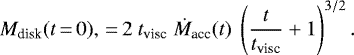 (6)
(6)
Stellar mass accretion rates have now been measured for multiple star-forming regions such as Lupus, Chamaeleon I, and Upper Sco (Alcalá et al. 2014, 2017; Manara et al. 2017, 2020). Based on these accretion rates we can calculate what the initial disk masses would have been, given the viscous timescale and the average age of the star-forming region.
To determine the initial disk masses of the models, our approach is as follows. We take four stellar mass accretion rates (4 × 10⁻¹², 4 × 10⁻¹¹, 2 × 10⁻⁹ and 10−8 M⊙ yr−1) that span the range of the observations in Lupus (see, e.g., Alcalá et al. 2014, 2017). As observations have shown that Ṁacc is correlated to M*, our selected Ṁacc represent the average accretion rates for stars with M* = 0.1, 0.2, 0.32, and 1.0 M⊙. Compared to Trapman et al. (2020) this includes one more set of models (M* = 0.2 M⊙). For these stellar mass accretion rates we calculate what the initial disk mass must have been for three different viscous timescales, assuming an average age of 1 Myr for Lupus. The viscous timescales are calculated for three values of the dimensionless viscosity αvisc = 10−2, 10−3, 10−4, assuming a characteristic radius of 10 AU (a choice that is discussed below) and a disk temperature Tdisk of 20 K (see, e.g., Eq. (37) in Hartmann et al. 1998)
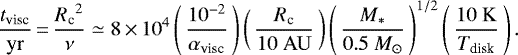 (7)
(7)
The resulting initial disk masses, 12 in total, are summarized in Table 1. Figure 1 shows how these disk masses decrease over time. In our analysis we exclude three models. Trapman et al. (2020) showed that the gas disk sizes measured from models with α = 10−2 and M* = [ 0.32, 1.0 ] M⊙ can be ruled out based on observed gas disk sizes in Lupus. We also exclude the model with M* = 1.0 M⊙ and α = 10−4, which has an initial disk mass of Mdisk = 2.6 × 10⁻¹ M⊙. At all points during its evolution, this model is factor of five more massive than the most massive disk observed in Lupus, but consistent with Class 0/1 disk masses (cf. Fig. A.1 in Trapman et al. 2020; see also Tychoniec et al. 2018, 2020; Tobin et al. 2020).
For the initial disk size we assume that disks start out small, with an initial characteristic disk size Rc (t = 0) = 10 AU. Recently, Trapman et al. (2020) showed that the observed gas outer radii of Class II disks in Lupus can be explained by viscously evolving disks that start out small (Rc(t = 0) = 10 AU) and that have a low viscosity (αvisc = 10−4−10−3). More importantly, they show that the bulk of the observed gas outer radii cannot be explained by disks that start out large (Rc (t = 0) ≥ 30 AU).
Observational constraints on the disk size of young Class 1 and 0 objects have only recently become available. In their VANDAM II survey, Tobin et al. (2020) presented ALMA 0.87 millimeter observations of 330 protostars in Orion at a resolution of ~ 0.′′1 (~ 40 AU in diameter). Their observations suggest that the majority of disks are initially small (~ 37−45 AU in radius), at least as seen in the emission of the millimeter dust. It is worth mentioning that their radii are defined as half of the full with at half maximum (FWHM) of a 2D Gaussian fit to the observations, which is not the same as the characteristic radius of the disk. For the gas there is similar evidence that disks start out small, albeitfrom a smaller sample. Maret et al. (2020) presented NOEMA observations of 16 Class 0 protostars as part of the CALYPSO large program. They found only two sources that show a Keplerian disk larger than ~ 50 AU. This suggests that stars with a large Keplerian disk at a young age, such as those found for VLA 1623 (Murillo et al. 2013), are uncommon. We therefore adopted an initial disk size of Rinit = 10 AU for our models.
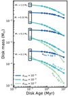 |
Fig. 1 Time evolution of the disk mass, Mdisk, of our models. Colors indicate the viscous alpha, αvisc, of the models. The black boxes show which stellar mass, and therefore accretion rate, was used to calculate the initial disk mass of the models (see Table 1). We note that we exclude models with αvisc = 10−2 for M* = [0.32, 1.0] M⊙ as the gas disk sizes of these models can be ruled out by observations of disks in Lupus (Trapman et al. 2020). We also note that models with M* = 1.0 M⊙ and αvisc = 10−4 are much more massive (Mgas ≳ 2 × 10⁻¹ M⊙) than the disks observed in Lupus (cf. Ansdell et al. 2016; see Fig. A.1 in Trapman et al. 2020). |
Initial conditions of our DALI models.
2.3 The DALI models
Using the initial conditions discussed previously we computed how Mdisk decreases and Rc increases over time. For ten points in the lifetime of the disk, starting at 0.1 Myr and ending at 10 Myr, we computed the current surface density Σgas(t) of the disk model.
We used the thermochemical code DALI to compute CO isotopolog abundances and line fluxes of our disk models. DALI is a 2D physical-chemical code that computes the thermal and chemical structure for a given physical disk structure. For each Σgas(t) a Monte Carlo radiative transfer calculation is used determine the dust temperature and the internal radiation field from UV- to mm-wavelengths. Next, the code computes atomic and molecular abundances by solving the time-dependent chemistry. The atomic and molecular excitation is then obtained using a non-LTE calculation. The heating and cooling balance is solved to calculate the gas temperature. These three steps were performed iteratively until a self-consistent solution is obtained. Raytracing of the model then yields line fluxes. For a more detailed description of the code we refer the reader to Appendix A of Bruderer et al. (2012).
To obtain a 2D (i.e., R, z) density structure for our models, we assumed that in the vertical direction the disk follows a Gaussian density distribution, as motivated by hydrostatic equilibrium (see, e.g., Chiang & Goldreich 1997). The height of the disk was assumed to follow a powerlaw of the form  , where hc is the opening angle at Rc and ψ is the flaring angle.
As grains grow larger they decouple from the gas and settle toward the midplane of the disk (see, e.g., Dubrulle et al. 1995; Dullemond & Dominik 2004, 2005; Mulders & Dominik 2012; Riols & Lesur 2018). The settling of large grains is included in our models in a simplified way by splitting the dust grains into two populations, following the approach in Andrews et al. (2011). Most of the dust mass (90%) is in large grains with sizes of 1–103 μm. These large grains follow the gas radially, but vertically they are confined to the midplane as their scale height is reduced by a factor χ = 0.2 with respect to the gas. A population of small grains (0.005–1 μm) make up the remaining 10% of the dust mass in the disk. These small grains follow the distribution of the gas both radially and vertically.
We assume that our disks encircle a typical T Tauri star, which we represent with a blackbody with effective temperature for Teff = 4000 K. A second blackbody with Teff = 10 000 K is added to simulate the excess UV radiation released by material accreted onto the star. To compute the luminosity of this second component we follow Kama et al. (2015) and assume that the gravitational potential energy of the accreted material is converted into radiation with a 100% efficiency. These parameters are summarized in Table 2. We note that stellar evolution is not included in our models. Including stellar evolution can affect CO chemistry and its chemical conversion. Especially the higher stellar luminosity early on will increase the disk temperature and reduce the amount of CO freeze out (see e.g., the observations presented in van’t Hoff et al. 2020a,b). A detailed study of the effect of stellar evolution on CO chemistry is available in Yu et al. (2016).
2.3.1 Isotopolog chemical network
For less abundant isotopologs of CO such as 13 CO, C18 O, and C17 O, isotope-selective photodissociation can have significant effect on their abundances (see, e.g., Visser et al. 2009; Miotello et al. 2014). Using the results from Visser et al. (2009), Miotello et al. (2014) expanded the standard chemical network of DALI, based on the UMIST 06 network (Woodall et al. 2007; Bruderer et al. 2012; Bruderer 2013), to include the isotope-selective photodissociation and chemistry of 13 CO, C18 O, and C17 O. The chemical network includes the formation of H2 on grains, freeze-out, thermal and nonthermal desorption of species, hydrogenation of simple species on ices, gas-phase reactions, photodissociation, X-ray- and cosmic-ray-induced reactions, polycyclic aromatic hydrocarbon (PAH) grain charge exchange and/or hydrogenation, and reactions with vibrationally excited H . A detailed description of the implementation of these reactions can be found in Appendix A.3.1 of Bruderer et al. (2012). A full description of the isotopolog chemical network can be found in Miotello et al. (2014). For the initial volatile carbon and oxygen abundances, typical ISM values of [C]/[H]ISM = 1.35 × 10⁻⁴, [O]/[H]ISM = 2.88 × 10⁻⁴ were used (Cardelli et al. 1996; Jonkheid et al. 2007; Woitke et al. 2009; Bruderer et al. 2012). We take the isotope ratios to be [12 C]/[13C] = 77 and [16 O]/[18O] = 560 (Wilson & Rood 1994).
Relevant for this work is that in the DALI chemical network CO is not further processed once it is frozen out on the grains. The only reaction included in the network that affects CO ice is desorption back into the gas phase.
DALI parameters of the physical model.
2.3.2 CO conversion through grain-surface chemistry
Recent observations have shown that a large fraction of protoplanetary disks have unexpectedly low 13CO and C18O line fluxes (see, e.g., Ansdell et al. 2016; Miotello et al. 2017; Long et al. 2017). Gas masses derived from these line fluxes using models that include freeze-out and photodissociation suggest that the bulk of the protoplanetary disks are gas poor, with gas-to-dust mass ratios (Δgd) on the order of Δgd ≈ 1−10. For a few disks the gas mass has been determined independently using HD (see, e.g., Bergin et al. 2013; McClure et al. 2016; Trapman et al. 2017; Kama et al. 2020). These observations suggest instead that CO is underabundant in disks (see, e.g., Favre et al. 2013; Du et al. 2015; Bergin et al. 2016; Kama et al. 2016; Zhang et al. 2019). This requires some process currently not accounted for that removes CO from the gas phase. Two such processes have been suggested: The first proposes that when CO freezes out on grain it can become locked up in larger bodies, preventing it from reentering the gas phase (see, e.g. Bergin et al. 2010, 2016; Du et al. 2015; Kama et al. 2016; Krijt et al. 2018, 2020). Radial drift of these larger bodies can move the frozen out CO to smaller radii (see, e.g. Booth et al. 2017). Several authors have also shown that grain-surface chemistry is capable of lowering the CO abundance in disks. In the gas collisions with He+ can break apart CO molecules, allowing the available carbon to be locked up in hydrocarbons such as CH4 and C2 H6 (see, e.g., Aikawa et al. 1997; Bergin et al. 2014; Schwarz et al. 2018). In the ice CO can be converted into other species such as CO2 and CH3OH on a timescale of several megayears (see, e.g., Bergin et al. 2014; Yu et al. 2016, 2017; Bosman et al. 2018; Schwarz et al. 2019).
Calculating the “chemical conversion of CO” requires a large chemical network. As expanding the network significantly increases the computation time of a thermochemical model, it is unfeasible to calculate the chemical conversion of CO for a large set of models. In this work we have instead implemented the chemical conversion of CO using an approximate description for CO gas and grain-surface chemistry based on the results of Bosman et al. (2018). The description simplifies the full chemical network in Bosman et al. (2018) by only tracing the main carbon carriers, meaning CO, CH3OH, CO2 and CH4. The chemistry is split up into the carrier species that have long (>104 yr) chemical timescales and intermediates, radicals and ions, which have a short, <100 yr, chemical timescales. The former are explicitly integrated while kinetic equilibrium is assumed for the latter. A more detailed description can be found in Appendix A in Krijt et al. (2020).
Using this approximate grain-surface chemistry, we recalculate the CO abundances computed by DALI. In doing so some thought has to be put in where in the disk our method gives an accurate approximation of the full chemical network in Bosman et al. (2018). Based on tests where the full chemistry is computed, we identify three boundaries beyond which the shielded midplane approximation is no longer valid: a low outward column of CO, the presence of oxygen in the gas phase, and a high temperature. The first is an outward column of CO of NCO, outward = 1016 cm−2 (see also van Dishoeck & Black 1988; Heays et al. 2017). The outward column is defined as the minimum of the vertical and radial external columns. In regions with a lower outward column CO can be photodissociated by UV photons and the CO abundance is set by the balance between photodissociation and chemistry, which is included in DALI.
The second boundary is related to the fraction of oxygen in the gas phase. The approximation assumes that all gas-phase oxygen directly transforms into OH ice where it can react with CO or H to form CO2 ice or H2O ice, respectively. The presence of atomic oxygen in the gas phase in the model indicates that photodissociation is still a significant driver of thechemistry. UV dissociation reactions will dissociate carbon carriers other than CO and push carbon back into the more photo-stable CO (see, e.g., van Dishoeck & Black 1988). Empirically we have found the boundary where 5% of the available oxygen exists as gas-phase O or OH encloses the region where in the full chemical network CO is transformed into other species (see Fig. 2).
Finally we also exclude the parts of the disk where Tgas > 35 K. Tests show that above this temperature the conversion of CO through grain-surface chemistry is negligible. At these temperatures CO is converted in CH4 in the gas phase (see, e.g., Aikawa et al. 1997; Schwarz et al. 2018). This is the dominant route above ~ 25 K and densities below ≲1010 cm−3. It becomes less and less effective with increasing temperature due to the lower sticking of atomic oxygen on grains (see Fig. 4 in Bosman et al. 2018). The increased time atomic oxygen spends in the gas phase results in the reformation of CO through reactions of O and OH with hydrocarbon radicals and ions, for example: CH + O → HCO+ → CO.
It should be noted that efficiency of gas-phase conversion of CO depends directly on rate at which CO can be destroyed by He+. Changes to the assumptions made to calculate this rate, for example increasing cosmic-ray ionization rate of He, could increase the efficiency of gas-phase CO conversion. It should also be noted that our chemical conversion of CO focuses on the reactions that result in CO no longer being the main carbon carrier in the disk. Other reactions that include CO do still occur both inside and outside our set boundaries (e.g., the formation of H2CO; see, e.g., Loomis et al. 2015; Öberg et al. 2017; Terwisscha van Scheltinga et al. 2021), but these reactions do not significantly affect CO being the predominant carbon carrier. To summarize, CO abundances are recalculated using the approximate grain-surface chemistry for regions in the disk where NCO, outward > 1016, ≤ 5% of [O] is in O(g)+OH(g) and Tgas ≤ 35 K. The abundances of the CO isotopologs 13CO and C18O are calculated by scaling their abundances by factor  , that is, by how much the 12CO abundance has decreased.
Figure 3 shows the effects of CO conversion through grain-surface chemistry on the CO abundances at 1, 3, and 10 Myr for one of our disk models. As discussed above, the CO abundances are only recalculated below the dashed black lines. At 1 Myr the CO abundance is still CO∕H2 ~ 10−4 and CO has not been depleted significantly. By 3 Myr the CO abundance has dropped to CO∕H2 ~ 5 × 10⁻⁵ higher up in the disk and CO∕H2 ~ 5 × 10⁻⁶ close to the midplane. For 13CO the effect of isotope-selective photodissociation is partly offset by the reaction 13 C + + 12 CO → 13 CO + 12 C + + 35 K, which is energetically favored toward the production of 13CO at low temperatures (see, e.g., Visser et al. 2009; Miotello et al. 2014 and references therein).
Having a lower abundance and lacking a back reaction similar to 13CO (see Eq. (20) in Miotello et al. 2014), C18O is much more affected by isotope-selective photodissociation. As a result, C18O is confined to a layer deeper in the disk. This can be seen in Fig. 3, with the 13CO 3–2 emitting region lying higher up in the disk, fully above the black contour. The C18O 3–2 emitting region lies closer toward the midplane and crosses the black contour. We can therefore expect the 13CO 3–2 flux not to be affected by the chemical conversion of CO, whereas the C18O 3–2 flux will be affected. After 10 Myr almost all of the available CO has been converted, with CO∕H2 ≲ 10−6 for the region where CO can be converted through cosmic-ray-driven chemistry. The 13CO and C18O emitting regions have moved inward and upward to regions of the disk that still have a high CO abundance.
In this work we raytrace the 13CO and C18O J = 3−2 lines, but tests show that the J = 2−1 lines show the same qualitative behavior (cf. Appendices B and C). As a rule of thumb if the J = 3−2 lines are optically thick, meaning that at early ages, when the disk is most massive, the 13CO 2–1 line is up to 5% fainter (in Jy km s−1) and the C18O 2–1 line is up to 15% fainter. If the J = 3−2 lines are optically thin, the J = 2−1 fluxes are up to 30% lower for both 13CO and C18O.
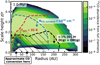 |
Fig. 2 CO abundance computed using the full chemical network in Bosman et al. (2018; see also Cridland et al. 2020) for the model with M* = 0.32 M⊙ and αvisc = 10−3 at 1 Myr. The chemistry was calculated using a ζcr = 10−16 s−1 to show where CO can be transformed. Taken from the same model, but with the chemistry calculated within DALI, the dashed blue line shows where the CO outward column is 1016 cm−2. The black contour shows where 5% of the total oxygen abundance is in OH(g) + O(g). The red contour shows where Tgas = 35 K. The hatched region below the three dashed lines shows where the CO abundance is recalculated using the approximate grain-surface chemistry. |
3 Results
3.1 CO isotopolog line fluxes: a viscously evolving disk
As the disk evolves viscously, the characteristic radius increases and the disk spreads out. At the same time the disk mass decreases as material is accreted onto the star. The left panel of Fig. 4 shows the surface density profile of the model with M* = 0.32 M⊙ and αvisc = 10−3, corresponding to an initial disk mass Mdisk(t = 0) = 10−2 M⊙, as it changes over time.
The middle panel of Fig. 4 shows the corresponding 13CO J = 3−2 azimuthally averaged intensity profile. Throughout most of the disk the 13CO emission is optically thick and decreases slowly with radius. In the outer part of the disk, at a radius between ~ 100 and 400 AU depending on the age of the model, the 13CO emission drops off rapidly. Comparing to the left panel in Fig. 4, this radius corresponds to a surface density of Σgas ≈ 10−3 g cm−2. Below this density, the 13CO column is no longer high enough to effectively self-shield and 13CO is rapidly removed from the disk beyond this radius.
As the 13CO emission is optically thick throughout almost all of the disk, the integrated 13CO flux is expected to increase over time as viscous expansion of the disk increases its emitting area. This is indeed what is seen in Fig. 5, where the top panel shows the integrated 13CO 3–2 flux as a function of disk age. 13CO intensity profiles of all of our models, shown in Appendix A, indicate that the 13CO emission is optically thick throughout the disk for all disk models with αvisc ≤ 10−3. Overall, the 13CO flux is therefore more of a disk size tracer than a disk mass tracer.
The rightmost panel of Fig. 4 shows the time evolution of the C18O intensity profile for the disk model with M* = 0.32 M⊙, αvisc = 10−3. The profile consists of two components: the inner ~90 AU is the emission of the bulk of the C18O in the disk, located just above the midplane. This emission is optically thick up to 3–5 Myr, after which the emission starts to become optically thin. The second component, visible beyond ~ 100 AU, is two orders of magnitude fainter than the first component. This emission is optically thin and originates from a lower abundance warm finger of C18O located higher up in the disk (see Fig. 2 in Miotello et al. 2014).
While the first component of the C18O emission is optically thick, the total C18O increases with age as can be seen in the bottom panel of Fig. 5. The total C18O 3–2 flux increases up to ~3 Myr. At this point the C18O emission within ~ 100 AU starts to become optically thin and the C18O integrated flux becomes a tracer of the disk mass instead of the disk size.
Whether the C18O integrated flux is predominantly optically thick and tracing the disk size or optically thin and tracing the disk mass is determined, to first order, by the mass and the size of the disk. For disk ages ≥1 Myr the C18O emission of our models is optically thin throughout the disk if M* ≤ 0.2 M⊙ and αvisc ≥ 10−3 (Mdisk(t = 1 Myr) ≤ 10−3 M⊙). However, higher mass disks (Mdisk(t = 1 Myr) around higher mass stars (M* ≥ 0.32 M⊙) or disks that have low turbulence (αvisc ≤ 10−4) instead have optically thick C18O 3–2 emission throughout most of the disk.
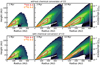 |
Fig. 3 Effect of the chemical conversion of CO on the CO abundance after 1, 3 and 10 Myr. The example model shown here has M* = 0.32 M⊙ and αvisc = 10−3. Top panels: CO abundances have been calculated using the DALI chemical network (see Sect. 2.3.1).Bottom panels: we have included the chemical conversion of CO into other species, as described in Sect. 2.3.2. Colors show the CO abundance with respect to H2, where white indicates CO/H2 ≤ 10−8. The dashed black line shows where ≤5% of the total amount of oxygen is in O(g)+OH(g), the gas temperature Tgas ≤ 35 K and outwardCO column is ≥1016 cm−2. Grain-surface chemistry is calculated below this black dashed line. Red contours show the 13 CO J = 3− 2 emitting region, enclosing 25 and 75% of the total 13CO flux. Similarly, the orange contours show the C18O J = 3− 2 emitting region. |
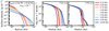 |
Fig. 4 Time evolution of the surface density profile (left panel), with the middle and right panel showing the corresponding 13CO J = 3−2 and C18O J = 3−2 intensity profiles, respectively. The model shown here has M* = 0.32 M⊙, α = 10−3 and Mdisk(t = 0) = 10−2 M⊙. The colors, going from red to blue, show different time steps. 13CO and C18O 3–2 intensity profiles for all models can be found in Appendix A. |
3.2 CO isotopolog line fluxes: effects of grain-surface chemistry
Before we compare our models to the observations, we first look at the effects of conversion of CO through grain-surface chemistry on CO isotopolog line fluxes. As lowering the CO abundance decreases the 13CO and C18O column densities, we expect the 13CO and C18O emission to become optically thin at an earlier disk age.
Figure 6 shows C18O and 13CO J = 3−2 integrated line fluxes for models with M* = 0.32 M⊙ and αvisc = [10−3, 10−4]. The line fluxes without grain-surface chemistry, presented earlier in Fig. 5, are included as dashed lines. Up to 1 Myr there is no discernible difference between the models with and without grain-surface chemistry, as it takes time for the chemistry to lower the gas-phase CO abundance. We note here that the timescale for the grain-surface chemistry depends directly on the assumed cosmic-ray ionization rate ζcr, which we have assumed to be ζcr = 1 × 10⁻¹⁷ s−1. For a higher ζcr the conversion of CO into other species will occur on a shorter timescale (see also Sect. 3.4).
For 13CO there is almost no difference when grain-surface chemistry is included even after 1 Myr. As can be seen in Fig. 3 the 13CO 3–2 emitting region lies almost completely above the region of the disk where CO can be transformed on the grains. Grain-surface chemistry has a larger effect on the C18O fluxes because the C18O 3–2 emitting region lies closer to the midplane, where the conversion of CO is most efficient (see, e.g., Fig. 3). For both αvisc = 10−3 and 10−4 the C18O 3–2 flux starts to decrease at a disk age of ~1.5 Myr. This indicates that the C18O emission is optically thin for a much larger disk masses (up to Mdisk ~ 2 × 10⁻² M⊙, cf. Fig. 1). At 10 Myr grain-surface chemistry has lowered the C18O 3–2 fluxes by a factor of ~2−3 compared to the model without CO conversion.
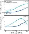 |
Fig. 5 13CO and C18O J = 3−2 line fluxes of a viscously evolving disk, shown in the top and bottom panel, respectively. Presented here are models with M* = 0.32 M⊙, αvisc = 10−3−10−4 that have an initial disk mass Mdisk(t = 0) = 2 × 10⁻³−2 × 10⁻² M⊙. We note that for these models CO conversion through grain-surface chemistry is not included. |
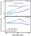 |
Fig. 6 13CO and C18O J = 3−2 line fluxes of a viscously evolving disk, shown in the top and bottom panel, respectively. Presented here are models with M* = 0.32 M⊙, αvisc = 10−3−10−4 that have an initial disk mass Mdisk(t = 0) = 2 × 10⁻³−2 × 10⁻² M⊙. A full overview of the model fluxes can be found in Fig. B.1. Solid lines show fluxes for models that include CO conversion through grain-surface chemistry. For comparison, dashed lines show fluxes for models without CO conversion as in Fig. 5. The red line highlights the age range of disks in the Lupus star-forming region. |
3.3 Comparing to the Lupus disk population
Recently Ansdell et al. (2016) have carried out an ALMA survey of the protoplanetary disk population in the Lupus star-forming region, in both continuum and 12CO, 13CO and C18O line emission (see also Ansdell et al. 2018). We examine whether the low 13CO and C18O 3–2 fluxes are compatible with viscous evolution.
Figure 7 shows the C18O and 13CO J = 3−2 integrated line fluxes of our models and observations of protoplanetary disks in Lupus (Ansdell et al. 2016; Yen et al. 2018). To have a useful comparison, we have aligned the models and observations based on total (estimated) disk mass. For the observations we use 100 × Mdust as a proxy for the disk mass. This is equivalent to assuming that disks have a gas-to-dust mass ratio Δgd = 100, the canonical value for the ISM. It is likely that radial drift of larger grains and their subsequent accretion onto the star causes disks to have a Δgd > 100. This would move the observations to the right in Fig. 7. We note, however, that substructures detected in the continuum (e.g., ALMA Partnership 2015; Andrews et al. 2016, 2018; van Terwisga et al. 2018; Long et al. 2018, 2019; Cieza et al. 2021) could halt the inward drift of large grains (see e.g., Pinilla et al. 2012; Dullemond et al. 2018). This is discussed in more detail in Sect. 4.2. In our analysis we exclude transition disks with a resolved inner cavity in the dust continuum as our models do no represent their disk structure (see van der Marel et al. 2018).
At the high mass end (Mdisk ≳ 5 × 10⁻³ M⊙) 13CO 3–2 is detected for all disks and C18O 3–2 is detected for most disks in Lupus. The observed range of 13CO fluxes is reasonably well reproduced by our models, although for individual objects the flux for the model with the corresponding mass might be a factor of two to four times higher. There are two disks, IM Lup (Sz 82) and HK Lup (Sz98) that are either significantly brighter or fainter than our models. These two disks are among the largest disks in Lupus. Interestingly, while these two disks are of similar size and dust mass, they differ in 13CO 3–2 flux by more than an order of magnitude, suggesting that the processes that affect the abundance of CO can be very different in two very similarly looking disks. We note that our models are aimed at reproducing the average protoplanetary disk and we do not expect them to reproduce outliers. In a similar study Trapman et al. (2020) showed that a larger initial disk size of 30–50 AU is required to reproduce the gas disk size of these large disks. The C18O 3–2 fluxes detected for the high mass disks are reproduced by the models within a factor of ~ 2 for most disks. Four of the massive disks in Lupus, slightly less than half of the disks in this mass range, are not detected in C18O 3–2. Our models overproduce these C18O upper limits by a factor of ~2−4, suggesting they either have a Δgd ≪ 100 or that they have lower C18O abundances than our models. The C18O fluxes in our models can be reduced by increasing the cosmic-ray ionization rate (see Sect. 3.4 and Fig. D.1).
For lower disk masses (5 × 10⁻⁴ M⊙ ≲ Mdisk ≲ 5 × 10⁻³ M⊙) the majority of disks in Lupus are still detected in 13CO but only a few are also detected in C18O. Here the 13CO fluxes of our models and the observations start to diverge. While the brightest observed 13CO fluxes are still reproduced by the models, there is up to an order of magnitude difference between the model 13CO fluxes and the bulk of the 13CO detections and the 13CO upper limits.
For C18O, comparing the models to the observations becomes more difficult due to the low number of C18O 3–2 detections in Lupus. The few C18O detections in this massrange are reproduced by the models. However, these are the same disks whose bright 13CO emission is also reproduced by the models. The C18O fluxes of the models do get low enough to match the observed C18O upper limits (~0.1 Jy km s−1), but only when the disk models are ~10 Myr old. This is much older than most disks in Lupus, which are estimated to be 1–3 Myr old.
Ansdell et al. (2016) stacked the disks that were detected in the continuum but not in 13CO 3–2 and C18O 3–2. First, stacking the 25 sources that were detected in the continuum and 13CO resulted in a mean continuum flux of 70 mJy, corresponding to a dust mass of ~5 × 10⁻⁵ M⊙, with a detected mean C18O 3–2 flux of 206 ± 31 mJy km s−1. Stacking the 26 sources detected in the continuum but not detected in both 13CO 3–2 and C18O 3–2 provided a much deeper mean C18O 3–2 upper limit of 42 mJy km s−1. We note that we have scaled the fluxes to a distance of 160 pc, the average distance to the Lupus clouds based on Gaia DR2 measurements (Gaia Collaboration 2018; Bailer-Jones et al. 2018), instead of the 200 pc used by Ansdell et al. (2016). This stacked upper limit lies a factor of five to ten lower than our model fluxes, similar to what was found for 13CO, suggesting that both 13CO 3–2 and C18O 3–2 fluxes are overproduced by our models, even if chemical conversion of CO is included.
For disks with Mdisk = 100 × Mdust ≲ 5 × 10⁻⁴ M⊙ only a handful of disks are detected in 13CO and none are detected in C18O. While the 13CO fluxes of the models have decreased for these lower gas masses, the model fluxes are still at least a factor of five higher than the observed 13CO upper limits. In comparison the C18O fluxes of the model have decreased with Mdisk and are consistent with the observed C18O upper limits.
To summarize, our viscously evolving disk models that include CO conversion are able to explain most observed 13CO and C18O fluxes for high mass disks (Mdisk ≳ 5 × 10⁻⁵ M⊙) in Lupus. For lower mass disks the model 13CO and C18O fluxes are up to an order of magnitude higher than what has been observed.
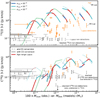 |
Fig. 7 13CO (top) and C18O (bottom) J = −2 line fluxes versus disk mass. Solid lines show models that include CO conversion through grain-surface chemistry. For comparison, dashed lines show the models without grain-surface chemistry. For the observations, shown in orange, we use Mgas ≃ 100 × Mdust as a proxy for the disk mass (see, e.g., Ansdell et al. 2016, 2018; Yen et al. 2018). Colors show models with different viscous alpha. Models with age between 1 and 3 Myr, the approximate age of Lupus, are highlighted in red. We note that in our models Mdisk decreases with time, meaning that time runs right to left in this figure for our models. Observations for which we only have an upper limit on the 13 CO or C18 O line flux are shown in gray. Stacked non-detections are shown in black (cf. Sect. 3.3). |
3.4 Cosmic-ray ionization rate required to match observed CO isotopolog fluxes
The previous Section showed that for disk masses below ~5 × 10⁻³ M⊙ the model 13CO and C18O fluxes are a factor of five to ten times higher than what is observed in Lupus. The cosmic-ray ionization rate ζcr is one of the main factors that determines the rate at which CO is converted into CO2, CH4 and CH3OH. In our models we have assumed a moderate ζcr ~ 10−17 s−1, comparable to the rate found in dense molecular clouds (see, e.g., Black et al. 1990). The cosmic-ray ionization rate in disks is highly uncertain, so it is possible that ζcr is higher, especially if activity from the young star at the center of the disk is contributing (see, e.g., Rab et al. 2017; Padovani et al. 2018). However, it should be noted that there is also evidence for a much lower cosmic-ray ionization rate in disks (ζcr~ 10−19−10−18 s−1) as a result of thedisk being shielded by the stellar magnetic field and disk winds (Cleeves et al. 2013, 2015). However, as reducing ζcr only decreases the effectiveness of the chemical conversion of CO we do not examine it here. Instead we examine if increasing ζcr would allow us to reproduce the observationsand what ζcr would be needed to do so in a 1–3 Myr time period. We focus on the mass range between Mdisk = 5 × 10⁻⁴ M⊙ and Mdisk = 10−2 M⊙ where the difference in fluxes between the models and the observations is the largest. Similarly, we focus on models with αvisc = 10−3 and M* = [0.2, 0.32] M⊙, which span a similar disk mass range.
Figure 8 shows the 13CO and C18O 3–2 fluxes after CO abundances were recalculated using a higher ζcr than is used in the models presented previously (ζcr = 1 × 10⁻¹⁷ s−1; see Table 2.) The 13CO 3–2 emission is only weakly dependent on the cosmic-ray ionization rate, with less than ~ 10% differences in flux. Again, this is due to the 13CO emitting region (z∕r ~ 0.2−0.35) being higher than the region ofCO removal (z∕r ≲ 0.15) In Sect. 4.1 we discuss alternative ways to reconcile the 13CO 3–2 observationswith our models.
The bottom panel of Fig. 8 shows that, in contrast to 13CO, increasing ζcr has a larger effect on the C18O fluxes, but not enough. Increasing ζcr from 1 × 10⁻¹⁷ s−1 to 5 × 10⁻¹⁷−10−16 s−1 is sufficient to explain almost all of the C18O detections for disks with 100 × Mdust ≳ 2 × 10⁻³ M⊙. However, the figure also shows that by increasing ζcr the C18O 3–2 fluxes can reduced to at most ~0.2 Jy km s−1, which is still a factor of ~2 higher than the observed C18O upper limits in Lupus. Moreover, the fluxes obtained from our models remain a factor of ~ 5 higher than the stacked C18O 3–2 upper limits. This indicates that increasing the amount of cosmic-ray ionization in our models by itself cannot explain the faintest C18O 3–2 fluxes.
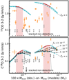 |
Fig. 8 Effect of the cosmic ray ionization rate on 13CO and C18O J = 3− 2 line fluxes, shown in the top and bottom panel respectively. Models shown here have αvisc = 10−3 and M* = [ 0.2, 0.32 ] M⊙. Solid light blue lines show the model line fluxes where CO conversion through grain-surface chemistry is calculated with a cosmic ray ionization rate ζcr = 1 × 10⁻¹⁷ s−1. For the black dashed lines ζcr is increased up to 5 × 10⁻¹⁶ s−1. The dashed blue line shows the upper limit of the effect of grain-surface chemistry, where we have removed all CO in the region of the disk where CO conversion by grain-surface chemistry is effective. Observations in Lupus are shown in orange if detected and in gray if an upper limit (Ansdell et al. 2016; Yen et al. 2018). The stacked non-detections are shown in black (see also Sect. 3.3). The red shaded lane highlights the age range of the Lupus star-formingregion. |
4 Discussion
4.1 Reproducing 13CO 3–2 line fluxes observed in Lupus
In Sect. 3.3 it was found that our models overproduce the 13CO 3–2 and C18O 3–2 observation in Lupus by a factor of five to ten for disks with Mdisk ≲ 5 × 10⁻³ M⊙. By increasing the cosmic-ray ionization rate from ζcr = 1 × 10⁻¹⁷ s−1 to 10−16 s−1 it is possible to decrease the C18O 3–2 fluxes of our models to within a factor of two of the observed upper limits. However, the 13CO 3–2 emission originates predominantly from a layer higher up in the disk where CO is not being efficiently converted into other species. As such, the 13CO 3–2 fluxes of our models remain a factor of 10−30 times higher than the observations, even after removing all CO from region of the disk where CO grain-surface chemistry is effective. Here, we examine the emitting regions of 13CO 3–2 and C18O 3–2 and we discuss processes that could reduce the 13CO and C18O fluxes to the point where they are in agreement with both detections and upper limits seen in observations.
Figure 9 shows an example of the 13CO and C18O emitting regions in a model with maximum CO conversion. The 13CO emitting region is located high up in the disk (z∕r ~ 0.25−0.4), fully above the region where CO can be removed (z∕r ≲ 0.15). The presence of oxygen in the gas phase in this layer indicates that it cannot be locked up efficiently in H2O, meaning it is available to react with the carbon released from the destruction of CO to reform CO (see also Schwarz et al. 2018). It should be noted a small amount of carbon can go into other molecules such as H2CO (e.g., Loomis et al. 2015; Öberg et al. 2017; Terwisscha van Scheltinga et al. 2021) and C2 H (e.g., Kastner et al. 2015; Bergin et al. 2016; Cleeves et al. 2018; Bergner et al. 2019; Miotello et al. 2019), but in this FUV dominated layer CO remains the main carbon carrier (see Fig. 18 in Schwarz et al. 2018). The C18O emitting region, shown in the bottom panel of Fig. 9 lies much deeper in the disk, at a height of z∕r ~ 0.18. With efficient CO conversion the C18O emitting region is very compact and extends only slightly above the oxygen-threshold. Unlike for 13CO it is therefore plausible that a slight change in for example the height of the disk will push the C18O abundant region below the oxygen-threshold, thus drastically reducing the observed C18O 3–2 fluxes. In the rest of this section we therefore focus on lowering the 13CO 3–2 fluxes, which are in stronger violation with the observations.
Knowing the location of the 13CO emission, we can discuss processes by which the emission can be reduced.
A colder disk
Given that the 13CO 3–2 emission is optically thick, a lower disk temperature could potentially explain the low 13CO 3–2 emission in Lupus. Lowering Tgas would decrease the brightness of the optically thick line. The temperature of a disk is predominantly set by its vertical structure. Our models all have the same height,  (see Sect. 2.3). In reality, however, it is unlikely that all disks have the same height. The vertical structure that is assumed in our disk models is thought to be a good representation of the average disk vertical structure, but there are only a few disks, biased toward high disk masses, for which the disk height has been estimated using the scattering surface observed in scattered light (see, e.g., Avenhaus et al. 2018; Garufi et al. 2020). It is therefore possible that lower mass disks are much flatter (hc ≪ 0.1), and therefore colder, than previously thought.
A lower scale height would also increase the fraction of CO in the disk that can be converted. Reducing the scale height of the disk would concentrate the mass in the shielded midplane, where the cosmic-ray-driven conversion of CO is efficient.
A colder disk cannot explain all of the disks observed to be underabundant in CO. The TW Hya disk is thought to be underabundant in CO by a factor of 10–100 (see, e.g., Favre et al. 2013; Du et al. 2015; Bergin et al. 2016; Kama et al. 2016; Trapman et al. 2017; McClure et al. 2020). This disk is also known to be much more flared (ψ ~ 0.3), and therefore warmer, than the disk models presented here (see, e.g., Kama et al. 2016; van Boekel et al. 2017; Schwarz et al. 2016; Calahan et al. 2021). Although anecdotal, the example of TW Hya shows that a colder disk cannot be the sole explanation for the low observed 13CO 3–2 fluxes (see also Fedele et al. 2016).
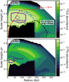 |
Fig. 9 13CO (top) and C18O (bottom) abundance structure (colors) and J = 3−2 emitting regions (purple contours) for an example disk model (M* = 0.32 M⊙, αvisc = 10−3 and a disk age of 1.5 Myr). The contours shown are the same as in Fig. 2. |
Smaller disks
Another way to explain the low 13CO 3–2 fluxes would be that disks are smaller than our models. Trapman et al. (2020) showed that our models are consistent with observed gas disk sizes in Lupus, measured from the extent of the 12 CO J = 2−1 emission. However, these observations are biased toward the most massive disks around the most massive stars in the Lupus disk population. Comparing their results with the observations presented in Fig. 7 reveals that there are only three disks below Mdisk = 3 × 10⁻³ M⊙ for which the gas disk size has been measured: Sz 133 (238 AU), Sz 65 (172 AU), and Sz 73 (103 AU). Of these, only Sz 73 has a 13CO flux that lies a factor of ~2 below the predictions of our models. For the remaining disks of similar or lower mass the gas disk size is unknown. Without knowing their gas disk size, it could be possible that the low 13CO fluxes can be explained by a compact gas disk.
The optically thick emitting region of our disk models with Mdisk ≲ 5 × 10⁻³ M⊙ has a radius of ~ 30−150 AU, depending on the mass and Rc of the disk model. The 13CO 3–2 flux scales with emitting area (F ∝ R2). To reduce the 13CO 3–2 flux of these models by a factor of 10−30 and bring them in line with the observations, the disk size has to be reduced by a factor of three to five, to ~ 10−50 AU. We note that this is the disk size as measured from the 13CO 3–2 emission. Trapman et al. (2019) found that the gas disk size measured from 12 CO is 30–35% larger than the gas disk size measured from 13CO, assuming that both 12CO and 13CO are optically thick. This would suggest that disks with dust masses ≲ 3 × 10⁻⁴ M⊙ need to have gas disk sizes on the order of ~40−70 AU as measured from 12 CO if small disks are the explanation for the low 13CO fluxes. It should be noted however that disks with similar 13CO flux can have very different gas disk sizes (e.g., Sz 129 (140 AU) and HK Lup (358 AU)), suggesting that 13CO might not always be optically thick and that compact disks might not be the sole explanation for the faint 13CO emission seen in observations. Deeper high resolution (≲ 0.′′2) 12 CO and 13CO observations of low mass disks are required to test this theory.
Vertical mixing
It is very likely that turbulence in protoplanetary disks mixes material both vertically and radially. Through vertical mixing the CO-rich material higher up in the disk would be moved down toward the midplane, where the CO can then be converted into other species via grain-surface chemistry. If the mixing timescale is much shorter than the lifetime of the disk the CO will be well mixed and the CO abundance higher up in the disk will match that of the CO-poor material close to the midplane (see, e.g., Willacy et al. 2006; Semenov & Wiebe 2011; Krijt et al. 2018, 2020).
Figure 10 shows the effect of vertical mixing on the 13CO and C18O 3–2 fluxes. Here we have approximated the effect of mixing by setting the CO abundance higher up in the disk equal to the mass-weighted average CO abundance in the region where we compute the grain-surface chemistry. To obtain such efficient mixing requires a mixing timescale that is much shorter than the disk age. Based on turbulent diffusion, Krijt et al. (2020) calculate a vertical mixing timescale of tz ≈ 2.5 × 10⁵ yr for one scale height at 30 AU assuming a turbulent strength corresponding to α = 10−4, which is also the lowest level of turbulence assumed in our models. We have also assumed that mixing goes up to the 13CO emitting layer at z∕r ~ 0.25−0.4.
Up to 3 Myr vertical mixing does not significantly affect the 13CO and C18O fluxes for the standard case of ζcr = 1 × 10⁻¹⁷ s−1. While the material in the upper layer of the disk is now well mixed with the material below, the grain-surface chemistry has not had enough time to decrease the mass-averaged CO abundance to the point where it has a noticeable effect on the isotopolog line fluxes. After 3 Myr both the 13CO flux has started to decrease rapidly and by 10 Myr the fluxes from the our models are at or below the level of the observed upper limits in Lupus.
The effect of mixing on the 13CO and C18O 3–2 fluxes is limited to how quickly the chemistry is able to decrease the mass-averaged CO abundance. It is therefore interesting to examine whether a combination of vertical mixing and a higher cosmic-ray ionization rate ζcr can explain the 13CO 3–2 observationsin Lupus within 1–3 Myr age of the region. We included vertical mixing in our models with ζcr = 5 × 10⁻¹⁷−10−16 s−1 and present the resulting fluxes in Fig. 10. With CO conversion now occurring at an increased rate, vertical mixing has a much larger impact at earlier disk ages. Within 3 Myr the model fluxes have decreased to the same level as the faintest 13CO and C18O detections and upper limits in Lupus. By combining vertical mixing with a high cosmic-ray ionization rate of ζcr = 5 × 10⁻¹⁷−10−16 s−1 we can explain all 13CO 3–2 and C18O 3–2 observationsin Lupus.
This is in agreement with recent results of Krijt et al. (2020), who investigated processes that have been invoked to explain low CO abundances inferred for disks, such as chemical conversion of CO, turbulent diffusion of gas and small grains and locking up CO in large bodies. They show that a combination of vertical mixing and the chemical conversion of CO can decrease the CO abundance to 10−6−10−5 up to z∕r ~ 0.2, which is the upper edge of their model. This is similar to the mass-weighted average CO abundance of the viscous disk models that reproduce the observed 13CO and C18O 3–2 upper limits (see Fig. 10). We should note however that to lower the 13CO flux mixing must be efficient up to at least z∕r ~ 0.3 (see Fig. 9). Krijt et al. (2020) also show that including the locking up of CO ice into larger bodies in addition to the chemical conversion of CO can further decrease the CO abundance to below 10−6 at z∕r ~ 0.2 for ζcr = 1 × 10⁻¹⁷ s−1. The combination of these processes could therefore potentially explain the low observed fluxes without having to invoke a high cosmic-ray ionization.
The effect of vertical mixing combined with the chemical conversion of CO is expected to lower the total volatile carbon abundance in the upper layers of the disk. Observations of atomic carbon in TW Hya indeed show evidence that the upper layer of the disk is carbon poor (see Kama et al. 2016), but there is insufficient observational evidence to show that this extends to all protoplanetary disks. Krijt et al. (2020) also find that vertical mixing and chemical conversion of CO leads to (C/O)gas > 1 in the upper layer of the disk (see their Fig. 10). This prediction is in agreement with the bright ring-shaped C2 H emission that has been detected in a number of disks (see, e.g., Kastner et al. 2015; Bergin et al. 2016; Cleeves et al. 2018; Miotello et al. 2019; Bergner et al. 2019). However, it should be noted that it is still unclear how the C2H emission is related to the total amount of carbon that has been removed from the disk (see e.g., the discussion in Miotello et al. 2019).
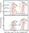 |
Fig. 10 13CO 3–2 model fluxes after applying vertical mixing (dash-dotted black lines) compared the observation in Lupus (orange markers). Upper limits are shown in gray. The stacked non-detections are shown in black (see also Sect. 3.3). Shown here are disk models with αvisc = 10−3 and M* = [ 0.2, 0.32 ] M⊙. For reference, the model fluxes without vertical mixing are shown in light blue. The dashed and dotted black lines show models where mixing is combined with higher cosmic-ray ionization rates (see also Sect. 3.4). The red shaded lane highlights the age range of the Lupus star-forming region. |
4.2 Alternative explanations
Assumed gas-to-dust mass ratio. In Sect. 3.3 we compared our models to observations of disks in Lupus. In this comparison we used Mdisk ≈ 100 × Mdust, which is equivalent to assuming that the disk has inherited the ISM gas-to-dust mass ratio of Δgd = 100. However, most of the dust mass in protoplanetary is made up of large grains, which are expected to radially drift inward where they are accreted onto the star. This process would lead to Δgd ≫ 100, with simulations of dust evolution in protoplanetary disks showing values as high as Δgd = 103−104 (see, e.g., Birnstiel et al. 2012). Increasing the assumed gas-to-dust mass ratio would shift the observations to the right in Fig. 7, as it would increase the gas mass we associate with each of the sources. While this could change which models the observations are compared to, it would not significantly affect our results. A small increase (Δgd = 200−300) might help the comparison between the observations and our models at the high mass end. The main effect of increasing Δgd would be increasing the gas mass threshold, currently Mdisk ≲ 5 × 10⁻³ M⊙, below whichwe require a higher cosmic-ray ionization rate to match our models to the observations (see also Fig. D.1).
We note here that lowering the gas-to-dust mass ratio of the observed sources to Δgd = 1−10 would also allow us to reproduce the observed 13CO and C18O fluxes with our models. This is in essence the same result as was obtained by Ansdell et al. (2016) and Miotello et al. (2017), who showed that gas masses derived from the 13CO and C18O fluxes suggest thatdisks have low gas-to-dust mass ratios. However, these lower gas masses would no longer be consistent with observed stellar mass accretion rates under the assumption of viscous evolution (see Manara et al. 2016).
On the other side of this comparison are the initial disk masses used for our models. As outlined in Sect. 2.2, the initial disk mass Mdisk(t = 0) is set by the stellar accretion rate Ṁacc, for which we took the representative Ṁacc for four stellar masses, M* = [ 0.1, 0.2, 0.32, 1.0 ] M⊙, from observations. As the observationsshow a spread in Ṁacc there should be a similar spread in Mdisk(t = 0). Changing the initial disk mass would, to first order, move the model curves to the left or right in Fig. 7. While the gas masses of both the models and observations can be varied to some degree, changing the gas masses alone cannot explain the order of magnitude difference between the 13CO fluxes of models and the observations.
The assumption of viscous evolution
Throughout this work we have assumed that protoplanetary disks evolve viscously and calculated the time evolution of 13CO and C18O 3–2 line fluxes based on this premise. However, it is also possible disk evolution is instead driven by magnetic disk winds. While a quantitative analysis of this scenario is beyond the scope of this work, we can discuss the expected differences. In our models we saw that the 13CO fluxes, and to some degree the C18O fluxes, increase with time while the disk mass instead decreases with time. This is attributed to a combination of the 13CO emission being mostly optically thick and the disk viscously spreading as it evolves. If disk evolution is instead driven by disk winds the disk is not expected to spread out and the 13CO and C18O line fluxes will not increase over time. Instead, the 13CO and C18O fluxes are expected to remain constant with time while the emission is optically thick. To drive the observed stellar mass accretion the disk mass has to decrease over time. At some point the 13CO and C18O emission will become optically thin and the line fluxes will start to decrease over time, similarly to what is seen for C18O at 2 Myr in Fig. 5. It might take more time for the emission to become optically thin because, in contrast to a viscously spreading disk, the disk mass is not distributed out over an increasingly larger area. Indeed, if disks start out small as suggested by observations (e.g. Maury et al. 2019; Tobin et al. 2020), it is possible that the 13CO emission remains optically thick as most of the mass is concentrated in a small area. To test whether disk evolution is driven by disk winds or by viscous spreading, future observations should focus on detecting and resolving the 12 CO, 13CO and C18O emission of the disks that make up the bulk of the disk population of star-forming regions spread over a wide age range.
5 Conclusions
In this workwe have used the thermochemical code DALI to run a series of viscously evolving disk models with initial disk masses based on observed stellar mass accretion rates. Using these models we examined how CO isotopolog line fluxes, commonly used as to measure disk gas masses, change over time in a viscously evolving disk. We also compared our models to 13CO J = 3−2 and C18O J = 3−2 observationsof disks in the Lupus star-forming region, to investigate if they are consistent with disks evolving viscously. Here we present our conclusions:
-
13CO and C18O 3–2 fluxes of viscously evolving disks increase over time due to the lines being optically thick and their optically thick emitting area increasing in size as the disk expands. Only for disks around stars with M* ≤ 0.2 M⊙ that evolve with a moderate amount of turbulence (αvisc ≥ 10−3) the C18O 3–2 emission is optically thin throughout the disk and the integrated C18O flux thus trace the disk mass.
-
Including the conversion of CO through grain-surface chemistry at <35 K does not affect the 13CO flux. Initially the C18O is also not affected, but from ~1 Myr onward it starts to decrease up to a factor of ~2−3 at 10 Myr. This also ensures that from ~1 Myr and onward C18O 3–2 emissiondecreases with time in a viscously evolving disk.
-
The observed 13CO 3–2 and C18O 3–2 line fluxes of the most massive disks (Mdisk ≳ 5 × 10⁻³ M⊙) in Lupus are consistent to within a factor of two with our viscously evolving disk models where CO is converted into other species through grain-surface chemistry, assuming a moderate cosmic-ray ionization rate ζcr ~ 10−17 s−1.
-
Increasing the cosmic-ray ionization rate to ζcr ≳ 5 × 10⁻¹⁷− 10−16 s−1 decreases the C18O fluxes to within a factor of ~2 of the observed upper limits for disks in Lupus with Mdisk ≲ 5 × 10⁻³ M⊙. Reproducing the stacked C18O upper limit observed in Lupus requires a lower average abundance, which could be obtained with efficient vertical mixing.
-
Our models overpredict the observed 13CO 3–2 fluxes by a factor of 10−30 for most disks with Mdisk ≲ 5 × 10⁻³ M⊙ because the 13CO 3–2 emission originates from a layer at z∕r ~ 0.25−0.4 (= 2.5−4 × hc for our models), which is much higher up than the region where CO can be efficiently converted into other species (z∕r ≲ 0.15).
-
Reproducing the 13CO 3–2 observations in Lupus requires both efficient vertical mixing and a higher cosmic-ray ionization rate, ζcr ~ 5 × 10⁻¹⁷−10−16 s−1. Alternatively, the observations can be explained if less massive (Mdust ≲ 3 × 10⁻⁵ M⊙) disks are either much flatter and colder or much smaller (RCO, 90% ~ 40−70 AU) than their more massive counterparts.
Our models show that the observed C18O fluxes in Lupus areconsistent with these disks having evolved viscously, if CO has been converted into other species under a high cosmic-ray ionization rate. The observed 13CO fluxes are also consistent with this picture, provided that the material in the disk is also well mixed vertically. However, alternative explanations for the low observed 13CO fluxes such as the disks being colder or smaller than assumed cannot be discarded based on current observations. Deeper observations that resolve the CO isotopolog emission of low mass disks are needed to conclusively demonstrate whether these disks are evolving viscously. Observing the products into which CO is being converted will be difficult as they are either frozen out or their emission lines lie in the infrared. However, with the James Webb Space Telescope it will be possible to search for CO2 and CH3OH ice at intermediate disk layers of edge-on disks or for CO2 gas in the inner disk (see, e.g., Bosman et al. 2017; Anderson et al. 2021 for a more detailed discussion).
Acknowledgements
We thank the referee for the useful comments that helped improve the manuscript. L.T. and M.R.H. are supported by NWO grant 614.001.352. A.D.B. acknowledges support from NSF Grant#1907653 and NASA grant XRP 80NSSC20K0259. G.R. acknowledges support from the Netherlands Organisation for Scientific Research (NWO, program number 016.Veni.192.233). G.R. also acknowledges an STFC Ernest Rutherford Fellowship (grant number ST/T003855/1). Astrochemistry in Leiden is supported by the Netherlands Research School for Astronomy(NOVA). All figures were generated with the PYTHON-based package MATPLOTLIB (Hunter 2007). This research made use of Astropy (http://www.astropy.org), a community-developed core Python package for Astronomy (Astropy Collaboration 2013, 2018).
Appendix A Model 13CO and C18O J = 3–2 intensity profiles
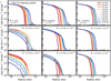 |
Fig. A.1 Time evolution of the 13CO J = 3−2 intensity profiles of our models, where colors denote different time steps. Each panel shows a different M* and αvisc. |
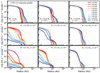 |
Fig. A.2 Time evolution of the 13CO J = 3−2 intensity profiles of our models, where colors denote different time steps. Each panel shows a different M* and αvisc. |
Appendix B Model 13CO and C18O J = 3–2 integrated fluxes
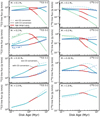 |
Fig. B.1 As Fig. 6, but showing the 13CO (left) and C18O (right) J = 3− 2 fluxes for all models. Colors indicate different αvisc. Models with and without CO conversion through grain-surface chemistry are shown with solid and dashed lines, respectively. The age range for disks in Lupus is highlighted in red. Few models show a significant decrease in 13CO line fluxes, except for models with αvisc = 10−2 that have low disk masses. The C18O line fluxes do show a decrease with age, especially at later disk ages. |
Appendix C Model 13CO and C18O J = 2–1 fluxes
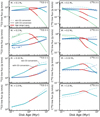 |
Fig. C.1 As Fig. B.1, but showing the 13CO (left) and C18O (right) J = 2− 1 fluxes for allmodels. We note that the range of the y-axes are the same as for Fig. B.1. |
Appendix D Comparing maximum CO conversion models to observed CO isotopolog line fluxes
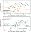 |
Fig. D.1 As Fig. 6, but now showing three sets of models. The dotted lines show the 13 CO (top) and C18O (bottom) J = 3−2 line fluxes for models with standard DALI chemistry, that is, without CO conversion. The solid lines show line fluxes for the models where CO has been chemically converted into other species, as described in Sect. 2.3.2. The dashed lines show line fluxes for models with maximal CO conversion, where we have removed all CO in the region where CO conversion through grain-surface chemistry occurs (see also Sect. 8). Observations in Lupus are shown in orange if detected and gray if an upper limit (Ansdell et al. 2016; Yen et al. 2018). Stacked non-detections are shown in black (see Sect. 3.3). |
References
- Aikawa, Y., Umebayashi, T., Nakano, T., & Miyama, S. M. 1997, ApJ, 486, L51 [NASA ADS] [CrossRef] [Google Scholar]
- Alcalá, J., Natta, A., Manara, C., et al. 2014, A&A, 561, A2 [NASA ADS] [CrossRef] [EDP Sciences] [Google Scholar]
- Alcalá, J., Manara, C., Natta, A., et al. 2017, A&A, 600, A20 [NASA ADS] [CrossRef] [EDP Sciences] [Google Scholar]
- ALMA Partnership (Brogan, C. L., et al.) 2015, ApJ, 808, L3 [NASA ADS] [CrossRef] [Google Scholar]
- Anderson, D. E., Blake, G. A., Cleeves, L. I., et al. 2021, ApJ, 909, 55 [NASA ADS] [CrossRef] [Google Scholar]
- Andrews, S. M., Wilner, D. J., Espaillat, C., et al. 2011, ApJ, 732, 42 [Google Scholar]
- Andrews, S. M., Wilner, D. J., Zhu, Z., et al. 2016, ApJ, 820, L40 [NASA ADS] [CrossRef] [Google Scholar]
- Andrews, S. M., Terrell, M., Tripathi, A., et al. 2018, ApJ, 865, 157 [Google Scholar]
- Ansdell, M., Williams, J. P., van der Marel, N., et al. 2016, ApJ, 828, 46 [Google Scholar]
- Ansdell, M., Williams, J. P., Manara, C. F., et al. 2017, AJ, 153, 240 [NASA ADS] [CrossRef] [EDP Sciences] [Google Scholar]
- Ansdell, M., Williams, J. P., Trapman, L., et al. 2018, ApJ, 859, 21 [Google Scholar]
- Armitage, P. J. 2015, ArXiv e-prints [arXiv:1509.06382] [Google Scholar]
- Astropy Collaboration (Robitaille, T. P., et al.) 2013, A&A, 558, A33 [NASA ADS] [CrossRef] [EDP Sciences] [Google Scholar]
- Astropy Collaboration (Price-Whelan, A. M., et al.) 2018, AJ, 156, 123 [Google Scholar]
- Avenhaus, H., Quanz, S. P., Garufi, A., et al. 2018, ApJ, 863, 44 [Google Scholar]
- Bailer-Jones, C. A. L., Rybizki, J., Fouesneau, M., Mantelet, G., & Andrae, R. 2018, AJ, 156, 58 [NASA ADS] [CrossRef] [Google Scholar]
- Balbus, S. A., & Hawley, J. F. 1991, ApJ, 376, 214 [NASA ADS] [CrossRef] [Google Scholar]
- Balbus, S. A., & Hawley, J. F. 1998, Rev. Mod. Phys., 70, 1 [Google Scholar]
- Barenfeld, S. A., Carpenter, J. M., Ricci, L., & Isella, A. 2016, ApJ, 827, 142 [Google Scholar]
- Barenfeld, S. A., Carpenter, J. M., Sargent, A. I., Isella, A., & Ricci, L. 2017, ApJ, 851, 85 [NASA ADS] [CrossRef] [Google Scholar]
- Benz, W., Ida, S., Alibert, Y., Lin, D., & Mordasini, C. 2014, in Protostars and Planets VI, eds. H. Beuther, R. S. Klessen, C. P. Dullemond, & T. Henning (Tucson: University of Arizona Press), 691 [Google Scholar]
- Bergin, E., Hogerheijde, M., Brinch, C., et al. 2010, A&A, 521, L33 [NASA ADS] [CrossRef] [EDP Sciences] [Google Scholar]
- Bergin, E. A., Cleeves, L. I., Gorti, U., et al. 2013, Nature, 493, 644 [NASA ADS] [CrossRef] [PubMed] [Google Scholar]
- Bergin, E., Cleeves, L. I., Crockett, N., & Blake, G. 2014, Faraday Discuss., 168, 61 [Google Scholar]
- Bergin, E. A., Du, F., Cleeves, L. I., et al. 2016, ApJ, 831, 101 [NASA ADS] [CrossRef] [Google Scholar]
- Bergner, J. B., Öberg, K. I., Bergin, E. A., et al. 2019, ApJ, 876, 25 [NASA ADS] [CrossRef] [Google Scholar]
- Béthune, W., Lesur, G., & Ferreira, J. 2017, A&A, 600, A75 [NASA ADS] [CrossRef] [EDP Sciences] [Google Scholar]
- Birnstiel, T., Klahr, H., & Ercolano, B. 2012, A&A, 539, A148 [NASA ADS] [CrossRef] [EDP Sciences] [Google Scholar]
- Bjerkeli, P., van der Wiel, M. H. D., Harsono, D., Ramsey, J. P., & Jørgensen, J. K. 2016, Nature, 540, 406 [NASA ADS] [CrossRef] [Google Scholar]
- Black, J. H., van Dishoeck, E. F., Willner, S. P., & Woods, R. C. 1990, ApJ, 358, 459 [NASA ADS] [CrossRef] [Google Scholar]
- Booth, R. A., Clarke, C. J., Madhusudhan, N., & Ilee, J. D. 2017, MNRAS, 469, 3994 [NASA ADS] [CrossRef] [Google Scholar]
- Borucki, W. J., Koch, D. G., Basri, G., et al. 2011, ApJ, 736, 19 [NASA ADS] [CrossRef] [Google Scholar]
- Bosman, A. D., Bruderer, S., & van Dishoeck, E. F. 2017, A&A, 601, A36 [NASA ADS] [CrossRef] [EDP Sciences] [Google Scholar]
- Bosman, A. D., Walsh, C., & van Dishoeck E. F. 2018, A&A, 618, A182 [NASA ADS] [CrossRef] [EDP Sciences] [Google Scholar]
- Bruderer, S. 2013, A&A, 559, A46 [NASA ADS] [CrossRef] [EDP Sciences] [Google Scholar]
- Bruderer, S., van Dishoeck, E. F., Doty, S. D., & Herczeg, G. J. 2012, A&A, 541, A91 [NASA ADS] [CrossRef] [EDP Sciences] [Google Scholar]
- Calahan, J., Bergin, E., Zhang, K., et al. 2021, ApJ, 908, 8 [Google Scholar]
- Cardelli, J. A., Meyer, D. M., Jura, M., & Savage, B. D. 1996, ApJ, 467, 334 [NASA ADS] [CrossRef] [Google Scholar]
- Cazzoletti, P., Manara, C. F., Baobab Liu, H., et al. 2019, A&A, 626, A11 [NASA ADS] [CrossRef] [EDP Sciences] [Google Scholar]
- Chiang, E. I., & Goldreich, P. 1997, ApJ, 490, 368 [NASA ADS] [CrossRef] [Google Scholar]
- Cieza, L. A., Ruíz-Rodríguez, D., Hales, A., et al. 2019, MNRAS, 482, 698 [Google Scholar]
- Cieza, L. A., González-Ruilova, C., Hales, A. S., et al. 2021, MNRAS, 501, 2934 [Google Scholar]
- Cleeves, L. I., Adams, F. C., & Bergin, E. A. 2013, ApJ, 772, 5 [Google Scholar]
- Cleeves, L. I., Bergin, E. A., Qi, C., Adams, F. C., & Öberg, K. I. 2015, ApJ, 799, 204 [NASA ADS] [CrossRef] [Google Scholar]
- Cleeves, L. I., Öberg, K. I., Wilner, D. J., et al. 2018, ApJ, 865, 155 [NASA ADS] [CrossRef] [Google Scholar]
- Cox, E. G., Harris, R. J., Looney, L. W., et al. 2017, ApJ, 851, 83 [Google Scholar]
- Cridland, A. J., Bosman, A. D., & van Dishoeck, E. F. 2020, A&A, 635, A68 [CrossRef] [EDP Sciences] [Google Scholar]
- de Valon, A., Dougados, C., Cabrit, S., et al. 2020, A&A, 634, L12 [NASA ADS] [CrossRef] [EDP Sciences] [Google Scholar]
- Dodson-Robinson, S. E., Evans, Neal J., I., Ramos, A., Yu, M., & Willacy, K. 2018, ApJ, 868, L37 [NASA ADS] [CrossRef] [Google Scholar]
- Du, F., Bergin, E. A., & Hogerheijde, M. R. 2015, ApJ, 807, L32 [Google Scholar]
- Dubrulle, B., Morfill, G., & Sterzik, M. 1995, Icarus, 114, 237 [NASA ADS] [CrossRef] [Google Scholar]
- Dullemond, C. P., & Dominik, C. 2004, A&A, 421, 1075 [NASA ADS] [CrossRef] [EDP Sciences] [Google Scholar]
- Dullemond, C. P., & Dominik, C. 2005, A&A, 434, 971 [NASA ADS] [CrossRef] [EDP Sciences] [Google Scholar]
- Dullemond, C. P., Birnstiel, T., Huang, J., et al. 2018, ApJ, 869, L46 [NASA ADS] [CrossRef] [EDP Sciences] [Google Scholar]
- Facchini, S., Birnstiel, T., Bruderer, S., & van Dishoeck E. F., 2017, A&A, 605, A16 [NASA ADS] [CrossRef] [EDP Sciences] [Google Scholar]
- Favre, C., Cleeves, L. I., Bergin, E. A., Qi, C., & Blake, G. A. 2013, ApJ, 776, L38 [NASA ADS] [CrossRef] [Google Scholar]
- Fedele, D., van Dishoeck, E. F., Kama, M., Bruderer, S., & Hogerheijde, M. R. 2016, A&A, 591, A95 [NASA ADS] [CrossRef] [EDP Sciences] [Google Scholar]
- Ferreira, J., Dougados, C., & Cabrit, S. 2006, A&A, 453, 785 [NASA ADS] [CrossRef] [EDP Sciences] [Google Scholar]
- Furuya, K., & Aikawa, Y. 2014, ApJ, 790, 97 [NASA ADS] [CrossRef] [Google Scholar]
- Gaia Collaboration (Brown, A. G. A., et al.) 2018, A&A, 616, A1 [NASA ADS] [CrossRef] [EDP Sciences] [Google Scholar]
- Garufi, A., Avenhaus, H., Pérez, S., et al. 2020, A&A, 633, A82 [CrossRef] [EDP Sciences] [Google Scholar]
- Hartmann, L., Calvet, N., Gullbring, E., & D’Alessio, P. 1998, ApJ, 495, 385 [NASA ADS] [CrossRef] [Google Scholar]
- Heays, A. N., Bosman, A. D., & van Dishoeck, E. F. 2017, A&A, 602, A105 [NASA ADS] [CrossRef] [EDP Sciences] [Google Scholar]
- Hunter, J. D. 2007, Comput. Sci. Eng., 9, 90 [NASA ADS] [CrossRef] [Google Scholar]
- Jonkheid, B., Dullemond, C. P., Hogerheijde, M. R., & van Dishoeck, E. F. 2007, A&A, 463, 203 [NASA ADS] [CrossRef] [EDP Sciences] [Google Scholar]
- Kama, M., Folsom, C. P., & Pinilla, P. 2015, A&A, 582, L10 [NASA ADS] [CrossRef] [EDP Sciences] [Google Scholar]
- Kama, M., Bruderer, S., van Dishoeck, E. F., et al. 2016, A&A, 592, A83 [NASA ADS] [CrossRef] [EDP Sciences] [Google Scholar]
- Kama, M., Trapman, L., Fedele, D., et al. 2020, A&A, 634, A88 [CrossRef] [EDP Sciences] [Google Scholar]
- Kastner, J. H., Qi, C., Gorti, U., et al. 2015, ApJ, 806, 75 [NASA ADS] [CrossRef] [Google Scholar]
- Krijt, S., Schwarz, K. R., Bergin, E. A., & Ciesla, F. J. 2018, ApJ, 864, 78 [NASA ADS] [CrossRef] [Google Scholar]
- Krijt, S., Bosman, A. D., Zhang, K., et al. 2020, ApJ, 899, 134 [Google Scholar]
- Long, F., Herczeg, G. J., Pascucci, I., et al. 2017, ApJ, 844, 99 [NASA ADS] [CrossRef] [Google Scholar]
- Long, F., Pinilla, P., Herczeg, G. J., et al. 2018, ApJ, 869, 17 [NASA ADS] [CrossRef] [Google Scholar]
- Long, F., Herczeg, G. J., Harsono, D., et al. 2019, ApJ, 882, 49 [Google Scholar]
- Loomis, R. A., Cleeves, L. I., Öberg, K. I., Guzman, V. V., & Andrews, S. M. 2015, ApJ, 809, L25 [NASA ADS] [CrossRef] [Google Scholar]
- Lynden-Bell, D., & Pringle, J. E. 1974, MNRAS, 168, 603 [NASA ADS] [CrossRef] [Google Scholar]
- Manara, C. F., Rosotti, G., Testi, L., et al. 2016, A&A, 591, L3 [NASA ADS] [CrossRef] [EDP Sciences] [Google Scholar]
- Manara, C. F., Testi, L., Herczeg, G. J., et al. 2017, A&A, 604, A127 [NASA ADS] [CrossRef] [EDP Sciences] [Google Scholar]
- Manara, C. F., Natta, A., Rosotti, G. P., et al. 2020, A&A, 639, A58 [CrossRef] [EDP Sciences] [Google Scholar]
- Maret, S., Maury, A. J., Belloche, A., et al. 2020, A&A, 635, A15 [NASA ADS] [CrossRef] [EDP Sciences] [Google Scholar]
- Maury, A. J., André, P., Testi, L., et al. 2019, A&A, 621, A76 [NASA ADS] [CrossRef] [EDP Sciences] [Google Scholar]
- McClure, M. K., Bergin, E. A., Cleevs, L. I., et al. 2016, ApJ, 831, 167 [NASA ADS] [CrossRef] [Google Scholar]
- McClure, M. K., Dominik, C., & Kama, M. 2020, A&A, 642, L15 [Google Scholar]
- Miotello, A., Bruderer, S., & van Dishoeck, E. F. 2014, A&A, 572, A96 [NASA ADS] [CrossRef] [EDP Sciences] [Google Scholar]
- Miotello, A., van Dishoeck, E., Williams, J., et al. 2017, A&A, 599, A113 [NASA ADS] [CrossRef] [EDP Sciences] [Google Scholar]
- Miotello, A., Facchini, S., van Dishoeck, E. F., et al. 2019, A&A, 631, A69 [NASA ADS] [CrossRef] [EDP Sciences] [Google Scholar]
- Mordasini, C. 2018, Handbook of Exoplanets, Planetary Population Synthesis (Berlin: Springer), 143 [Google Scholar]
- Morton, T. D., Bryson, S. T., Coughlin, J. L., et al. 2016, ApJ, 822, 86 [Google Scholar]
- Mulders, G. D., & Dominik, C. 2012, A&A, 539, A9 [NASA ADS] [CrossRef] [EDP Sciences] [Google Scholar]
- Murillo, N. M., Lai, S.-P., Bruderer, S., Harsono, D., & van Dishoeck, E. F. 2013, A&A, 560, A103 [NASA ADS] [CrossRef] [EDP Sciences] [Google Scholar]
- Öberg, K. I., Guzmán, V. V., Merchantz, C. J., et al. 2017, ApJ, 839, 43 [NASA ADS] [CrossRef] [Google Scholar]
- Padovani, M., Ivlev, A. V., Galli, D., & Caselli, P. 2018, A&A, 614, A111 [NASA ADS] [CrossRef] [EDP Sciences] [Google Scholar]
- Pascucci, I., Testi, L., Herczeg, G., et al. 2016, ApJ, 831, 125 [NASA ADS] [CrossRef] [Google Scholar]
- Pinilla, P., Birnstiel, T., Ricci, L., et al. 2012, A&A, 538, A114 [NASA ADS] [CrossRef] [EDP Sciences] [Google Scholar]
- Pontoppidan, K. M., Blake, G. A., & Smette, A. 2011, ApJ, 733, 84 [NASA ADS] [CrossRef] [Google Scholar]
- Pringle, J. E. 1981, ARA&A, 19, 137 [Google Scholar]
- Rab, C., Güdel, M., Padovani, M., et al. 2017, A&A, 603, A96 [NASA ADS] [CrossRef] [EDP Sciences] [Google Scholar]
- Riols, A., & Lesur, G. 2018, A&A, 617, A117 [NASA ADS] [CrossRef] [EDP Sciences] [Google Scholar]
- Rosotti, G. P., Clarke, C. J., Manara, C. F., & Facchini, S. 2017, MNRAS, 468, 1631 [NASA ADS] [Google Scholar]
- Schwarz, K. R., Bergin, E. A., Cleeves, L. I., et al. 2016, AJ, 823, 91 [Google Scholar]
- Schwarz, K. R., Bergin, E. A., Cleeves, L. I., et al. 2018, ApJ, 856, 85 [NASA ADS] [CrossRef] [Google Scholar]
- Schwarz, K. R., Bergin, E. A., Cleeves, L. I., et al. 2019, ApJ, 877, 131 [NASA ADS] [CrossRef] [Google Scholar]
- Semenov, D., & Wiebe, D. 2011, ApJS, 196, 25 [Google Scholar]
- Shakura, N. I., & Sunyaev, R. A. 1973, A&A, 24, 337 [NASA ADS] [Google Scholar]
- Tabone, B., Cabrit, S., Bianchi, E., et al. 2017, A&A, 607, L6 [NASA ADS] [CrossRef] [EDP Sciences] [Google Scholar]
- Terwisscha van Scheltinga, J., Hogerheijde, M. R., Cleeves, L. I., et al. 2021, ApJ, 906, 111 [Google Scholar]
- Tobin, J. J., Sheehan, P. D., Megeath, S. T., et al. 2020, ApJ, 890, 130 [Google Scholar]
- Trapman, L., Miotello, A., Kama, M., van Dishoeck, E. F., & Bruderer, S. 2017, A&A, 605, A69 [NASA ADS] [CrossRef] [EDP Sciences] [Google Scholar]
- Trapman, L., Facchini, S., Hogerheijde, M. R., van Dishoeck, E. F., & Bruderer, S. 2019, A&A, 629, A79 [NASA ADS] [CrossRef] [EDP Sciences] [Google Scholar]
- Trapman, L., Rosotti, G., Bosman, A. D., Hogerheijde, M. R., & van Dishoeck, E. F. 2020, A&A, 640, A5 [EDP Sciences] [Google Scholar]
- Turner, N. J., Fromang, S., Gammie, C., et al. 2014, Protostars and Planets VI (Tucson: University of Arizona Press), 411 [Google Scholar]
- Tychoniec, Ł., Tobin, J. J., Karska, A., et al. 2018, ApJS, 238, 19 [NASA ADS] [CrossRef] [Google Scholar]
- Tychoniec, Ł., Manara, C. F., Rosotti, G. P., et al. 2020, A&A, 640, A19 [CrossRef] [EDP Sciences] [Google Scholar]
- van Boekel, R., Henning, T., Menu, J., et al. 2017, ApJ, 837, 132 [NASA ADS] [CrossRef] [Google Scholar]
- van der Marel, N., Williams, J. P., Ansdell, M., et al. 2018, ApJ, 854, 177 [Google Scholar]
- van Dishoeck, E. F. & Black, J. H. 1988, ApJ, 334, 771 [NASA ADS] [CrossRef] [Google Scholar]
- van’t Hoff, M. L. R., van Dishoeck, E. F., Jørgensen, J. K., & Calcutt, H. 2020a, A&A, 633, A7 [CrossRef] [EDP Sciences] [Google Scholar]
- van’t Hoff, M. L. R., Harsono, D., Tobin, J. J., et al. 2020b, ApJ, 901, 166 [CrossRef] [Google Scholar]
- van Terwisga, S. E., van Dishoeck, E. F., Ansdell, M., et al. 2018, A&A, 616, A88 [NASA ADS] [CrossRef] [EDP Sciences] [Google Scholar]
- Vernet, J., Dekker, H., D’Odorico, S., et al. 2011, A&A, 536, A105 [NASA ADS] [CrossRef] [EDP Sciences] [Google Scholar]
- Visser, R., van Dishoeck, E. F., & Black, J. H. 2009, A&A, 503, 323 [NASA ADS] [CrossRef] [EDP Sciences] [Google Scholar]
- Weingartner, J. C., & Draine, B. 2001, ApJ, 548, 296 [NASA ADS] [CrossRef] [Google Scholar]
- Willacy, K., Langer, W., Allen, M., & Bryden, G. 2006, ApJ, 644, 1202 [NASA ADS] [CrossRef] [Google Scholar]
- Williams, J. P., Cieza, L., Hales, A., et al. 2019, ApJ, 875, L9 [Google Scholar]
- Wilson, T. L.,& Rood, R. 1994, ARA&A, 32, 191 [Google Scholar]
- Winn, J. N., & Fabrycky, D. C. 2015, ARA&A, 53, 409 [Google Scholar]
- Woitke, P., Kamp, I., & Thi, W.-F. 2009, A&A, 501, 383 [NASA ADS] [CrossRef] [EDP Sciences] [Google Scholar]
- Woodall, J., Agúndez, M., Markwick-Kemper, A., & Millar, T. 2007, A&A, 466, 1197 [NASA ADS] [CrossRef] [EDP Sciences] [Google Scholar]
- Yen, H.-W., Koch, P. M., Manara, C. F., Miotello, A., & Testi, L. 2018, A&A, 616, A100 [NASA ADS] [CrossRef] [EDP Sciences] [Google Scholar]
- Yu, M., Willacy, K., Dodson-Robinson, S. E., Turner, N. J., & Evans, Neal J., I. 2016, ApJ, 822, 53 [NASA ADS] [CrossRef] [Google Scholar]
- Yu, M., Evans, Neal J., I., Dodson-Robinson, S. E., Willacy, K., & Turner, N. J. 2017, ApJ, 841, 39 [NASA ADS] [CrossRef] [Google Scholar]
- Zhang, K., Bergin, E. A., Schwarz, K., Krijt, S., & Ciesla, F. 2019, ApJ, 883, 98 [NASA ADS] [CrossRef] [Google Scholar]
- Zhu, Z., & Stone, J. M. 2018, ApJ, 857, 34 [NASA ADS] [CrossRef] [Google Scholar]
All Tables
All Figures
|
Fig. 1 Time evolution of the disk mass, Mdisk, of our models. Colors indicate the viscous alpha, αvisc, of the models. The black boxes show which stellar mass, and therefore accretion rate, was used to calculate the initial disk mass of the models (see Table 1). We note that we exclude models with αvisc = 10−2 for M* = [0.32, 1.0] M⊙ as the gas disk sizes of these models can be ruled out by observations of disks in Lupus (Trapman et al. 2020). We also note that models with M* = 1.0 M⊙ and αvisc = 10−4 are much more massive (Mgas ≳ 2 × 10⁻¹ M⊙) than the disks observed in Lupus (cf. Ansdell et al. 2016; see Fig. A.1 in Trapman et al. 2020). |
| In the text | |
|
Fig. 2 CO abundance computed using the full chemical network in Bosman et al. (2018; see also Cridland et al. 2020) for the model with M* = 0.32 M⊙ and αvisc = 10−3 at 1 Myr. The chemistry was calculated using a ζcr = 10−16 s−1 to show where CO can be transformed. Taken from the same model, but with the chemistry calculated within DALI, the dashed blue line shows where the CO outward column is 1016 cm−2. The black contour shows where 5% of the total oxygen abundance is in OH(g) + O(g). The red contour shows where Tgas = 35 K. The hatched region below the three dashed lines shows where the CO abundance is recalculated using the approximate grain-surface chemistry. |
| In the text | |
|
Fig. 3 Effect of the chemical conversion of CO on the CO abundance after 1, 3 and 10 Myr. The example model shown here has M* = 0.32 M⊙ and αvisc = 10−3. Top panels: CO abundances have been calculated using the DALI chemical network (see Sect. 2.3.1).Bottom panels: we have included the chemical conversion of CO into other species, as described in Sect. 2.3.2. Colors show the CO abundance with respect to H2, where white indicates CO/H2 ≤ 10−8. The dashed black line shows where ≤5% of the total amount of oxygen is in O(g)+OH(g), the gas temperature Tgas ≤ 35 K and outwardCO column is ≥1016 cm−2. Grain-surface chemistry is calculated below this black dashed line. Red contours show the 13 CO J = 3− 2 emitting region, enclosing 25 and 75% of the total 13CO flux. Similarly, the orange contours show the C18O J = 3− 2 emitting region. |
| In the text | |
|
Fig. 4 Time evolution of the surface density profile (left panel), with the middle and right panel showing the corresponding 13CO J = 3−2 and C18O J = 3−2 intensity profiles, respectively. The model shown here has M* = 0.32 M⊙, α = 10−3 and Mdisk(t = 0) = 10−2 M⊙. The colors, going from red to blue, show different time steps. 13CO and C18O 3–2 intensity profiles for all models can be found in Appendix A. |
| In the text | |
|
Fig. 5 13CO and C18O J = 3−2 line fluxes of a viscously evolving disk, shown in the top and bottom panel, respectively. Presented here are models with M* = 0.32 M⊙, αvisc = 10−3−10−4 that have an initial disk mass Mdisk(t = 0) = 2 × 10⁻³−2 × 10⁻² M⊙. We note that for these models CO conversion through grain-surface chemistry is not included. |
| In the text | |
|
Fig. 6 13CO and C18O J = 3−2 line fluxes of a viscously evolving disk, shown in the top and bottom panel, respectively. Presented here are models with M* = 0.32 M⊙, αvisc = 10−3−10−4 that have an initial disk mass Mdisk(t = 0) = 2 × 10⁻³−2 × 10⁻² M⊙. A full overview of the model fluxes can be found in Fig. B.1. Solid lines show fluxes for models that include CO conversion through grain-surface chemistry. For comparison, dashed lines show fluxes for models without CO conversion as in Fig. 5. The red line highlights the age range of disks in the Lupus star-forming region. |
| In the text | |
|
Fig. 7 13CO (top) and C18O (bottom) J = −2 line fluxes versus disk mass. Solid lines show models that include CO conversion through grain-surface chemistry. For comparison, dashed lines show the models without grain-surface chemistry. For the observations, shown in orange, we use Mgas ≃ 100 × Mdust as a proxy for the disk mass (see, e.g., Ansdell et al. 2016, 2018; Yen et al. 2018). Colors show models with different viscous alpha. Models with age between 1 and 3 Myr, the approximate age of Lupus, are highlighted in red. We note that in our models Mdisk decreases with time, meaning that time runs right to left in this figure for our models. Observations for which we only have an upper limit on the 13 CO or C18 O line flux are shown in gray. Stacked non-detections are shown in black (cf. Sect. 3.3). |
| In the text | |
|
Fig. 8 Effect of the cosmic ray ionization rate on 13CO and C18O J = 3− 2 line fluxes, shown in the top and bottom panel respectively. Models shown here have αvisc = 10−3 and M* = [ 0.2, 0.32 ] M⊙. Solid light blue lines show the model line fluxes where CO conversion through grain-surface chemistry is calculated with a cosmic ray ionization rate ζcr = 1 × 10⁻¹⁷ s−1. For the black dashed lines ζcr is increased up to 5 × 10⁻¹⁶ s−1. The dashed blue line shows the upper limit of the effect of grain-surface chemistry, where we have removed all CO in the region of the disk where CO conversion by grain-surface chemistry is effective. Observations in Lupus are shown in orange if detected and in gray if an upper limit (Ansdell et al. 2016; Yen et al. 2018). The stacked non-detections are shown in black (see also Sect. 3.3). The red shaded lane highlights the age range of the Lupus star-formingregion. |
| In the text | |
|
Fig. 9 13CO (top) and C18O (bottom) abundance structure (colors) and J = 3−2 emitting regions (purple contours) for an example disk model (M* = 0.32 M⊙, αvisc = 10−3 and a disk age of 1.5 Myr). The contours shown are the same as in Fig. 2. |
| In the text | |
|
Fig. 10 13CO 3–2 model fluxes after applying vertical mixing (dash-dotted black lines) compared the observation in Lupus (orange markers). Upper limits are shown in gray. The stacked non-detections are shown in black (see also Sect. 3.3). Shown here are disk models with αvisc = 10−3 and M* = [ 0.2, 0.32 ] M⊙. For reference, the model fluxes without vertical mixing are shown in light blue. The dashed and dotted black lines show models where mixing is combined with higher cosmic-ray ionization rates (see also Sect. 3.4). The red shaded lane highlights the age range of the Lupus star-forming region. |
| In the text | |
|
Fig. A.1 Time evolution of the 13CO J = 3−2 intensity profiles of our models, where colors denote different time steps. Each panel shows a different M* and αvisc. |
| In the text | |
|
Fig. A.2 Time evolution of the 13CO J = 3−2 intensity profiles of our models, where colors denote different time steps. Each panel shows a different M* and αvisc. |
| In the text | |
|
Fig. B.1 As Fig. 6, but showing the 13CO (left) and C18O (right) J = 3− 2 fluxes for all models. Colors indicate different αvisc. Models with and without CO conversion through grain-surface chemistry are shown with solid and dashed lines, respectively. The age range for disks in Lupus is highlighted in red. Few models show a significant decrease in 13CO line fluxes, except for models with αvisc = 10−2 that have low disk masses. The C18O line fluxes do show a decrease with age, especially at later disk ages. |
| In the text | |
|
Fig. C.1 As Fig. B.1, but showing the 13CO (left) and C18O (right) J = 2− 1 fluxes for allmodels. We note that the range of the y-axes are the same as for Fig. B.1. |
| In the text | |
|
Fig. D.1 As Fig. 6, but now showing three sets of models. The dotted lines show the 13 CO (top) and C18O (bottom) J = 3−2 line fluxes for models with standard DALI chemistry, that is, without CO conversion. The solid lines show line fluxes for the models where CO has been chemically converted into other species, as described in Sect. 2.3.2. The dashed lines show line fluxes for models with maximal CO conversion, where we have removed all CO in the region where CO conversion through grain-surface chemistry occurs (see also Sect. 8). Observations in Lupus are shown in orange if detected and gray if an upper limit (Ansdell et al. 2016; Yen et al. 2018). Stacked non-detections are shown in black (see Sect. 3.3). |
| In the text | |
Current usage metrics show cumulative count of Article Views (full-text article views including HTML views, PDF and ePub downloads, according to the available data) and Abstracts Views on Vision4Press platform.
Data correspond to usage on the plateform after 2015. The current usage metrics is available 48-96 hours after online publication and is updated daily on week days.
Initial download of the metrics may take a while.