| Issue |
A&A
Volume 633, January 2020
|
|
|---|---|---|
| Article Number | A148 | |
| Number of page(s) | 17 | |
| Section | Extragalactic astronomy | |
| DOI | https://doi.org/10.1051/0004-6361/201936185 | |
| Published online | 23 January 2020 | |
Deriving star cluster parameters with convolutional neural networks
II. Extinction and cluster-background classification
1
Vilnius University Observatory, Saulėtekio av. 3, 10257 Vilnius, Lithuania
e-mail: jonas.bialopetravicius@ff.vu.lt, jonas.bialopetravicius@gmail.com
2
Center for Physical Sciences and Technology, Saulėtekio av. 3, 10257 Vilnius, Lithuania
Received:
26
June
2019
Accepted:
19
November
2019
Context. Convolutional neural networks (CNNs) have been established as the go-to method for fast object detection and classification of natural images. This opens the door for astrophysical parameter inference on the exponentially increasing amount of sky survey data. Until now, star cluster analysis was based on integral or resolved stellar photometry, which limit the amount of information that can be extracted from individual pixels of cluster images.
Aims. We aim to create a CNN capable of inferring star cluster evolutionary, structural, and environmental parameters from multiband images and to demonstrate its capabilities in discriminating genuine clusters from galactic stellar backgrounds.
Methods. A CNN based on the deep residual network (ResNet) architecture was created and trained to infer cluster ages, masses, sizes, and extinctions with respect to the degeneracies between them. Mock clusters placed on M 83 Hubble Space Telescope images utilizing three photometric passbands (F336W, F438W, and F814W) were used. The CNN is also capable of predicting the likelihood of the presence of a cluster in an image and quantifying its visibility (S/N).
Results. The CNN was tested on mock images of artificial clusters and has demonstrated reliable inference results for clusters of ages ≲100 Myr, extinctions AV between 0 and 3 mag, masses between 3 × 10³ and 3 × 10⁵ M⊙, and sizes between 0.04 and 0.4 arcsec at the distance of the M 83 galaxy. Real M 83 galaxy cluster parameter inference tests were performed with objects taken from previous studies and have demonstrated consistent results.
Key words: methods: data analysis / methods: statistical / techniques: image processing / galaxies: individual: M 83 / galaxies: clusters: general
© ESO 2020
1. Introduction
Observational astronomy is a favorable field for computer vision applications and currently also experiences the accelerating uptake of convolutional neural networks (CNNs). These methods have drastically improved various object recognition tasks from natural images, such as object classification and detection (Russakovsky et al. 2015). Just in the past year there have been numerous applications of CNNs in astrophysics, including galaxy shape estimation (Ribli et al. 2019), supernovae detection (Reyes et al. 2018), and radio source morphology classification (Wu et al. 2019). Such progress strongly motivates the adaptation of CNNs in star cluster analysis. Furthermore, CNNs perform inference by processing all pixels of an image, which is beneficial for the parameter derivation task as demonstrated by Whitmore et al. (2011), who used pixel-to-pixel variations to infer cluster ages.
In Paper I (Bialopetravičius et al. 2019) we implemented a CNN-based algorithm to simultaneously derive age, mass, and size of clusters in the low signal-to-noise ratio (S/N) regime. The algorithm was applied to M 31 clusters, cataloged by The Panchromatic Hubble Andromeda Treasury (PHAT) survey. We find that even when including information from all pixels and using accurate flux calibrations, interstellar extinction still plays a major role in influencing the results of parameter inference.
Numerous previous studies have explored physical parameter inference by taking into account the extinction problem, but these works were focused on the cases of resolved stellar or integrated cluster photometry. Among these are works by Bridžius et al. (2008), who used analytically integrated stellar luminosities, Fouesneau & Lançon (2010) and de Meulenaer et al. (2013, 2014), who used stochastically sampled stellar luminosities according to the stellar initial mass function (IMF), and SLUG, developed by Krumholz et al. (2015), which is one of the most mature codes in stochastic cluster population simulation and inference.
In this work we extend the CNN architecture proposed in Paper I to allow the inference of the interstellar extinction of a cluster directly from images. With an eye toward automated star cluster detection, we also explore indicators of cluster presence in images. The outputs of the network are modified to infer multiple cluster parameters jointly, which allows the degeneracies between them to be expressed in the outputs of the network, instead of relying on single-point estimates. This is especially useful when visualizing and dealing with age-extinction degeneracies.
We used the M 83 galaxy Hubble Space Telescope (HST) survey (Blair et al. 2014), which covers the entire disk of this face-on galaxy in a number of passbands. This allows us to investigate the effects of extinction in a variety of dense and sparse environments. Previous studies of the M 83 star cluster population have been based on aperture photometry; for example, Ryon et al. (2015) covered the whole galactic disk, Bastian et al. (2011) studied a smaller part of the galaxy in detail, and Harris et al. (2001) covered its central region. We trained the CNN on realistic mock observations and tested on mock clusters; we also validated our method on the aforementioned real cluster catalogs.
We also experimented with the renormalization of image fluxes for each passband separately when training the network, suggesting that precise photometric calibrations may not be necessary to derive star cluster parameters. This was done in the vein of Dieleman et al. (2015), in which JPEG color images are used to classify galaxies, achieving reliable results. This brings the approach of analysis of astronomical images closer to the methods used on natural images, which rarely have accurate flux calibrations.
The paper is organized as follows. Section 2 provides details about the M 83 survey data, the mock cluster bank construction, the added new parameters, and training data preparation. Section 3 describes the proposed CNN and its training methodology. Section 4 presents the results of testing the method on mock clusters and validating on real M 83 clusters previously studied using integral photometry. Section 5 discusses the CNN parameter inference results in an astrophysical context.
2. Data
2.1. M 83 mosaics
The M 83 mosaic project data observed by the HST Wide Field Camera 3 (WFC3; Blair et al. 2014; Dopita et al. 2010) was obtained from the Mikulski Archive for Space Telescopes1. We used stacked, defect-free mosaic images of 7 WFC3 fields, which are calibrated photometrically (pixel values are in counts per second) and astrometrically (with available world coordinate system information). The details of image processing are provided by Blair et al. (2014).
The mosaics cover the whole extent of the galaxy, from the dense center to its sparse outskirts where stellar background contamination is low. For the analysis we selected wide passband images that cover the whole galaxy without gaps: F336W, F438W, and F814W. All three mosaics are of the same size and in a tangential projection with a common scale (0.04 arcsec/pixel).
In Paper I the M 31 images were masked for saturated stars and extended objects to prevent unreliable CNN training. The distance to the M 31 galaxy is 785 kpc (McConnachie et al. 2005); however the distance to M 83 is 4.5 Mpc (Thim et al. 2003), therefore only a few saturated stars are visible. Because the area covered by extended objects in comparison to genuine stellar backgrounds is negligible, we decided to skip the masking step altogether and used all of the available mosaic area when selecting backgrounds for artificial clusters.
2.2. Mock cluster generation
Mock clusters were generated with different ages, masses, sizes, and affected by various levels of extinction. A fixed metallicity of Z = 0.03 (Hernandez et al. 2019) and standard extinction law with RV = AV/E(B − V) = 3.1 were assumed. To generate a cluster, its parameters were sampled independently of each other either from continuous (for mass and rh) or discrete (for age and AV) ranges. For a cluster to be included into the bank it also had to be brighter than a defined magnitude limit as discussed below to create suitable data for network training. We note that we did not perform grid sampling of cluster parameters, in which all possible permutations of their discrete values are combined, which would be computationally expensive, and, as further results show, not necessary for the network to learn cluster features based on a limited number of examples.
The age of each cluster was drawn with a uniform probability from the logarithmic range of log(t/yr) = [6.6, 10.1] with a step of 0.05 dex, which corresponds to 71 discrete ages in the isochrone bank. Mass for each cluster was drawn with a uniform probability from the logarithmic range of log(M/M⊙) = [3.5, 5.5] as a floating point number. The age and mass ranges were chosen to cover the majority of M 83 clusters studied by Bastian et al. (2011). Extinction was drawn with a uniform probability from the range of AV = [0.0, 3.0] mag with a step of 0.1 mag, which corresponds to 31 discrete extinctions in the isochrone bank. We define rh as the radius of a circle on the sky enclosing half of the stars of a cluster. The spatial distributions of stars were drawn from the Elson-Fall-Freeman (EFF, Elson et al. 1987) profile, which is defined as follows:

The parameters a and γ were drawn with a uniform probability from logarithmic ranges of [0.04, 1.2] and [2.05, 8.0] respectively as floating point numbers, such that rh is within the limits of [0.04, 0.4] arcsec. These values at the assumed distance of M 83 (Thim et al. 2003, 4.5 Mpc) roughly correspond to real cluster sizes (rh) in M 83 (Bastian et al. 2011).
The stars of the clusters were generated as follows. Given the initial mass, M, of a cluster, star masses were sampled according to the Kroupa (2001) IMF from Padova PARSEC isochrones2 (Bressan et al. 2012, release 1.2S), obtaining the absolute star magnitudes for passbands F336W, F438W, and F814W. Then, the absolute magnitudes were transformed to apparent magnitudes at the distance of M 83 (Thim et al. 2003, 4.5 Mpc) and converted to the WFC3 camera counts per second for the three passbands using calibrations provided by Dressel (2012). Finally, the spatial 2D positions of stars were generated by sampling their distances from the center of the cluster according to the EFF profile (with given a and γ values) and then distributing them symmetrically around the center.
The GalSim package (Rowe et al. 2015) was used to draw the individual stars of the clusters using TinyTim-generated3 point spread functions (PSFs; Krist et al. 2011) for each of the three passbands. Every star in the cluster was drawn separately for each passband using the appropriate PSF scaled by the flux of the star in counts per second. For a single cluster this produces three images, which can then be visualized as either RGB pictures or given to a CNN as 3D (width × height × passband) arrays. Artificial clusters were then placed on backgrounds cut from the M 83 mosaics. See Figs. 1 and 2 for examples of the generated mock clusters.
 |
Fig. 1. Examples of generated mock clusters placed on a real background image, which is the same for all panels. The ages of the clusters are shown top of each panel. The mass and size, rh, values are varied as shown on the axes; extinction AV = 0 mag. The intensity scale of the images was normalized with the arcsinh function within identical pixel value limits for each image. The yellow circles represent rh, obs values (rh convolved with the PSF). The value of the visibility, i.e., S/N proxy, is shown on the bottom left of each image for fainter objects with visibility < 100. Image sizes are 64 × 64 pixels (2.6 × 2.6 arcsec) or ∼60 × 60 pc at the distance of M 83. In the images red corresponds to passband F814W, green to F438W, and blue to F336W. |
To explore the photometric properties of the cluster bank, we show integrated color–color and color–magnitude diagrams in Fig. 3. The magnitudes depicted were obtained solely from integrating the total flux of mock clusters and therefore are an idealized case, which does not take into account the variations of background and spatial positions of stars. The only source of stochastic effects in such a case is IMF sampling. The panels are dedicated to illustrate the influence of age, extinction, and mass present in the bank. The effects of these parameters are in different directions in the color-color and color-magnitude space. The oldest clusters are red (panel a) and low-luminosity (panel e) objects. Clusters with high extinction are reddened (panel b), and the lowest mass clusters are faintest (panel g).
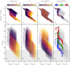 |
Fig. 3. Integrated color-color and color-magnitude diagrams of 50 000 generated mock clusters of the training bank and ∼7000 faint clusters. The color coding represents different ages (a, e), extinctions (b, f), and masses (c, g). Their values are as noted on the color bars on top. The last column (d, h) shows distributions of AV < 0.2 mag star clusters filtered by three mass ranges as specified on the color bar on top. The SSP tracks centered on the specified masses are shown as black curves. The shaded area below the dashed line represents the F814W magnitude limit used to filter out faint clusters. |
The last column (Fig. 3, panels d and h) shows distributions of star clusters filtered by mass and by extinction. The simple stellar population (SSP) tracks centered on the specified masses are shown as black curves. In both, color-color and color-magnitude space, it can be seen that lower mass clusters are more widely distributed because of the stochastic IMF sampling. The effects of mass on cluster magnitude can be seen again in Fig. 3h as vertical shifts of the SSP tracks.
This means that a point in color-color and color-magnitude space cannot uniquely map to a point in cluster parameter space. This is worsened by stochastic IMF sampling effects and results in degeneracies that any parameter inference method has to deal with. In cases like this any additional sources of information, such as individual image pixel values, are welcome.
Faint objects with mF336W > 24 mag, mF438W > 23.5 mag, and mF814W > 23 mag were not included in the final cluster bank because of their low signal, designed to mimic age, mass, and extinction selection effects existing in magnitude limited real cluster samples. As adding these extremely faint clusters to real backgrounds would result in mock images that are below the detection limit, the CNN would be forced to learn the parameters of a cluster on what effectively is just a plain background image. Therefore, magnitude cuts applied are necessary to provide the CNN with a balanced dataset. For the F814W band this is illustrated by the shaded gray area in Fig. 3. See the bottom left corner of panel d in Figs. 1 and 2 for examples of such barely visible clusters.
2.3. Mock cluster properties
Samples of artificial clusters were generated with the described parameters and placed on real backgrounds of M 83. In order to realistically model photon noise the following steps were applied. A cutout image of an M 83 background from a random position in the mosaics is selected and its median value is determined. This median is then added to the image of an artificial cluster, multiplied by the exposure time to get photon counts, and then each pixel is sampled from a Poisson distribution, with its mean set to the value of the pixel. The median is then subtracted back from this image, the real background image is added, and photon counts are transformed back to counts per second.
We also define a cluster visibility parameter, constructing this parameter to approximate S/N in such a way that higher values would be assigned to clusters that stand out relative to their stochastic stellar backgrounds. This parameter is defined as follows:

where fc is the integral flux of the cluster within its rh, obs, while σb is the standard deviation of the pixel values of the background in a 25 pix (1 arcsec) radius aperture, and n is the number of pixels within rh, obs. In this case rh, obs is the rh value of the cluster increased to account for PSF size, which has the largest effect on the most compact clusters. A mock cluster with visibility = 1 has mean flux per pixel approximately equal to the value of the standard deviation of a background it is placed on.
See Figs. 1 and 2 for a variety of visibility values of clusters, shown as yellow text in the corner of each image, where AV is up to 1 mag. See Fig. 4 for samples of clusters with the full range of extinction (AV up to 3 mag) used in this study to illustrate the effect of background crowding on visibility. It can be seen that the values of visibility correlate well with the ability to resolve clusters by eye, which is the best tool for cluster detection up to date.
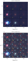 |
Fig. 4. Examples of generated mock clusters with varying ages and extinctions on real background images. The masses of the clusters are log10(M/M⊙) = 4.5, their sizes are log 10(rh/arcsec) = −0.7. The images are normalized as in Fig. 1. Top panel: clusters superimposed on a sparse background, bottom panel: same clusters superimposed on a denser background. The visibility value is indicated on the bottom left of each image. The sizes of the images are 64 × 64 pix. |
We note that for real clusters it is not possible to infer properties of background covered by the light of a cluster, however by placing mock objects into backgrounds, we can compute the visibility parameter beforehand and train the network to infer it from the data of real observations.
2.4. Training data preparation
To minimize the influence of photometric image calibration accuracy, the counts per second of each passband of the image of a cluster were individually normalized to the mean of 0 and standard deviation of 1. These were then rescaled with the arcsinh function. The resulting images were 64 × 64 pixels in size, which correspond to 2.6 × 2.6 arcsec or 60 × 60 pc at the distance of M 83 (Thim et al. 2003, 4.5 Mpc). Examples of the generated clusters with different ages, masses, and sizes, and without extinction, covering most of the parameter space, are shown in Fig. 1. A series of different examples (star position and mass sampling), but with extinction AV = 1 mag, are shown in Fig. 2. We generated 50 000 such images of mock clusters as a training sample for the CNN. The backgrounds have also been precomputed for efficiency resulting in 80 000 cutouts that were combined with the cluster images.
3. Convolutional neural network
3.1. Architecture
Following the work in Paper I, the ResNet-50 (He et al. 2016) architecture was used as a basis for our CNN. In addition, a series of modifications were made to the CNN to accommodate the different survey images, the higher number of predicted parameters, and the degeneracies between them. See Fig. 5 and Table 1 for details on the structure of the modified CNN.
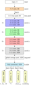 |
Fig. 5. Block diagram of the CNN. The three-channel input image of a cluster passes through the network top to bottom; the output result are age, extinction, mass, size, the cluster-background class classc/b, and visibility. All blocks with sharp corners depict single layers, while blocks with rounded corners are groupings of layers. The number on the left indicates how many times the group is repeated sequentially and the name on the right corresponds to the layer names in Table 1. The blocks with non-white backgrounds are parts of the network with optimizable parameters. The last number in each row is the number of output channels from that layer. “ReLU” indicates the locations in the network where rectified linear activations are applied between blocks. |
Designed 50-layer CNN based on the ResNet architecture.
In Paper I we used a method by Dieleman et al. (2015) to rotate the input image multiple times and pass it through the same convolutional layers; to simplify the network we omitted this step. The input image size was decreased to 64 × 64 pixels to account for the smaller angular size of the clusters due to the more distant galaxy. Three input channels were used corresponding to the F336W, F438W, and F814W passbands.
In Paper I, the parameters of the cluster were predicted via linear output layers by treating their prediction as a regression problem. This meant that each parameter was predicted independently. However, this approach is no longer viable owing to age-extinction degeneracies and age, extinction, and mass selection effects (shown in Fig. 3).
Therefore, we predicted all of the parameters on a grid; the positions on this grid correspond to the parameter values. This essentially transforms the regression problem into classification, allowing the network to predict each parameter in multiple locations of the parameter space, properly representing some degenerate cases such as low extinction and old age being just as likely as high extinction and young age.
Figure 6 depicts the four output layer activations. We grouped age, extinction, and mass into a single output layer to allow the degeneracies between these parameters to be expressed in the network architecture itself. This was done by predicting them as activations on a 3D grid, with 20 bins for age, 10 for extinction, and 14 for mass. When flattened, this results in a softmax layer with K = 2800 neurons. For classc/b K = 2 neurons were used to encode the likelihood of the presence of a cluster in the image. For the remaining parameters single-dimensional grids were used, resulting in K = 14 neurons for size and K = 20 for visibility.
 |
Fig. 6. Illustration of the activations in the output layers of the CNN. While training the CNN, target activation values are provided as a 3D Gaussian distribution for age, extinction, and mass (centered on true values as denoted by the red dot) and as 1D Gaussian distributions for rh (the blue line) and visibility (the red line). classc/b is represented as a value of 0 or 1. During inference the network produces similar outputs, examples of which are depicted in Figs. 8 and 20. |
Each of the four groups of output parameters were represented as softmax activations,

where z is the activations of a whole layer, and i specifies the index of a neuron (position on the parameter grid). The network was implemented with Keras4 and TensorFlow5 packages.
3.2. Training and inference
When training the network, we wish at the same time to infer both, classc/b, which indicates the presence of a cluster, and the astrophysical parameters of the cluster. To that end, learning the classc/b parameter was modeled as a simple binary classification task. The network is trained on batches of 512 images, half of which are images of backgrounds, and the other half are images of backgrounds combined with clusters as described in Sect. 2.2. We set classc/b = 0 for the images with only background, while we set classc/b = 1 for the samples with clusters.
In addition, for background images we zero out the training loss gradients for all cluster parameters. In effect this causes gradient updates to be derived only from the classc/b and visibility parameters, both of which are set to 0, indicating that the background contains no cluster. Training proceeds by sampling from M 83 backgrounds (∼25 000 images) and the cluster bank (50 000 mock clusters) separately, combining the cluster and background images on the fly, effectively giving us over 109 unique training samples.
The usual way to encode real-valued parameters as bins is called one-hot encoding. The parameter space is divided into bins and the bin at the position of the parameter’s value is set to 1. This array is then passed as a target vector, y, for the network. One-hot encoding is ideal for categorical classification, where only one of the target bins is true at a time. However, for binned real-valued parameters this has the unfortunate side-effect of penalizing bins far away from the target just as much as bins nearby to it. The way we solved this is by inserting a Gaussian distribution centered on the true value of the parameter (see Fig. 6). For the case of rh and visibility this is a simple 1D Gaussian, with a standard deviation equal to 0.5 the width of a bin. For age, mass, and AV a 3D Gaussian was used, with a standard deviation equal to 0.25 the width of a bin.
To obtain parameter estimates from this network we need a way to transform the output activations of the network back into single-point estimates that can then be analyzed. The 1D and 3D histograms, depicted in Fig. 6, need to be “unfolded”. This was done by finding the bin with the highest value in the histogram, which represents the most likely set of parameters inferred by the network, and calculating a weighted average within a radius of 3 bin widths. In effect this produces an output that is a real-valued, single-point estimate in between the bins instead of a discrete-valued estimate. Examples of inference results on mock and real clusters with both the raw activation outputs and the derived single-point estimates are shown in Figs. 8 and 20.
For computing the training gradients for the network the categorical cross-entropy loss function was used, that is,

where σ(z)i is the activation of the neuron, as described in Eq. (3), and yi is the target output for the given training cluster image.
The Adam optimizer (Kingma & Ba 2014) was used to calculate the gradients at each step of training. We experimented with various learning rates, starting from 0.1 down to 0.0001, with the learning rate decaying down to 0.0001 at the final iteration of training for all experiments. The learning rate of 0.01 gave the best performance on the mock validation set, so this was the value used for the final training of the network. The best CNN model was selected by picking the training iteration during which the CNN’s loss was the lowest on the validation set. The training accuracy track of the classc/b parameter for the resulting model is shown in Fig. 7. This is the only parameter for which accuracy can be meaningfully calculated because the other parameters are encoded as Gaussian distributions.
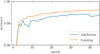 |
Fig. 7. Binary classification accuracy metric for classc/b on the training (orange) and validation (blue) sets during the course of CNN training. |
3.3. Output activations and stochastic effects
Three types of stochastic effects play a major role in the variation of CNN-inferred cluster parameters: 1) stellar mass sampling, 2) star spatial position randomization, and 3) background field. We combine stellar mass and position sampling into one stochastic factor as a property of the cluster itself, while leaving the background choice as a property of its environment. We study both effects separately by generating 100 different clusters with fixed parameters and placing them on the same background and placing the same cluster on 100 different backgrounds.
Figure 8 shows the influence of stochastic effects on the inference results of mock clusters. The left column shows clusters with log10(M/M⊙) = 5.0, extinctions AV = 0.5, 1.5, 2.5 mag, and log(t/yr) = 7.5, 8.5, 9.5. The right column shows clusters with AV = 0.5 mag, log10(M/M⊙) = 4.0, 4.5, 5.0, and the same ages. Cluster sizes are fixed at log10(rh/arcsec) = −0.6 for all cases. The top row shows the results of inference when stellar IMF sampling and spatial positions are varied while holding the cluster parameters constant. The middle row shows the results of inference when background images are varied while using the same cluster image. The cyan circles correspond to the true values of parameters. The grayscale colormaps are raw CNN outputs for one specific case and the magenta circles show 100 single-point estimates obtained for different random cases. The bottom row shows visualizations of the clusters with fixed background in the same format as Fig. 4. The visibility parameter value is shown on the bottom left of each image. We note that the CNN predicts ages, masses, and extinctions as one 3D cube, while the outputs shown are marginalized either over mass (left column) or extinction (right column).
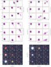 |
Fig. 8. Influence of stochastic effects on mock cluster inference results. Left column: clusters with log10(M/M⊙) = 5.0 and varied extinction and age. Right column: clusters with AV = 0.5 mag and varied mass and age. Cluster sizes are fixed at log10(rh/arcsec) = −0.6 for all cases. Top row: results of inference when stellar IMF sampling and spatial positions are varied while holding the cluster parameters constant. Middle row: results of inference when background images are varied while using the same cluster image. The cyan circles correspond to the true values of parameters. The grayscale colormaps are raw CNN outputs (activations over the parameter space) for one specific mock cluster case, while magenta circles show 100 single-point estimates obtained for different random cases. Bottom row: visualizations of the clusters with fixed background in the same format as in Fig. 4. |
In Fig. 8 it can be seen that the inference results for clusters with high visibility are all tightly packed for both types of stochastic effects (top and middle rows). This applies for both the spread of the CNN activation maps (grayscale) and the single-point estimates on different cluster images (magenta dots).
However, as clusters get fainter, and especially when they disappear into the background, the spread of activation maps (grayscale) and single-point estimates (magenta dots) get wider. Background variability has a significantly larger influence on the spread of parameter estimates than stellar sampling effects.
It is worth noting that for old clusters CNN output activations are elongated, attempting to represent age-extinction degeneracies. For a small number of cases bimodal solutions are obtained. However, for cases where clusters are completely invisible both activations and single-point estimates can end up tightly packed. This highlights the importance of the visibility parameter.
We note that less than 1% of the mock clusters show the bimodal distribution of activations. About 20% of the mock sample shows an extended unimodal distribution, while the rest of the results are symmetric and unimodal. Therefore, selecting the highest activation and obtaining single-point estimates from it is a viable approach, as that captures most of the information present in the CNN outputs.
For some clusters a systematic bias of the inference results can be observed, where the spread of activations would not sufficiently explain cluster misclassifications. This mainly occurs for the barely visible clusters, where only cluster sampling is varied. This implies that with a sufficiently difficult background and for a faint cluster, its parameter estimates may not be reliable and uncertainties may be underestimated.
However, Fig. 8 also illustrates the possibility to quantify the uncertainties of single inference results either from the extent of activation maps or by sampling random backgrounds, adding them to the image of a cluster, and rerunning inference. The former can produce tightly packed (underestimated) activation maps for some high-uncertainty samples, making them unreliable for low-visibility scenarios. The latter can also introduce additional effects, depending on the used background sampling method and the tendency to overestimate the uncertainties on real clusters, since the background effects would get doubled. In subsequent sections the single-point estimates are analyzed with respect to inferred parameter accuracy and the age-extinction degeneracy.
4. Results
4.1. Tests on mock clusters
To test the performance of the CNN, we built a separate bank of 5000 artificial clusters. Their parameters were drawn from the same distributions as described in Sect. 2.2. The backgrounds for these mock clusters were also sampled from the used M 83 mosaic, making sure that they are not the same as the backgrounds used for training. The inferred parameter values were obtained as described in Sect. 3.2.
The differences between CNN-derived single-point estimates of age, mass, extinction, and size versus true parameters are shown in Fig. 9. The spread of errors is visualized as a hexagonal density map with the count bins scaled logarithmically to highlight the spread of outliers. The dashed lines represent the error bounds containing 95% of the inference results for each parameter. We note that because of magnitude cuts introduced in the mock cluster bank, discussed in Sect. 2.2, the parameter distributions are not uniform. For example, there are relatively fewer low-mass, old-age clusters. In all of the panels, the clusters that are classified as much younger than the true given values are shown as red points, while the clusters classified as much older are highlighted as blue.
 |
Fig. 9. True and derived parameter values of test mock clusters visualized as a hexagonal density map. The bins are scaled logarithmically. Panels show comparisons for (a) age, (b) mass, (c) AV, and (d) rh. The dashed lines highlight the area containing 95% of the clusters. The red dots represent the clusters that were misclassified as younger than the real age values, while the blue dots represent clusters misclassified as older. |
Figure 9a shows no significant difference between the true and derived age values for log10(t/yr) < 8 and the distribution for all ages is symmetrical along the diagonal. The 95% of all inference results deviate < 0.9 dex from the true values, as shown by the dashed lines. Starting at log10(t/yr) = 8 and above a large scatter in both directions, toward older and younger ages, can be seen.
Figure 9c shows the true and derived AV values. The 95% of all inference results deviate < 1.4 dex from the true values, as shown by the dashed lines. The highlighted blue and red clusters are classified as having significantly higher and lower extinction, respectively. This can be explained by the age-extinction degeneracy, as older clusters with low extinction are hard to distinguish from younger clusters with high extinction, and vice versa, when using only three photometric passbands.
In Figs. 3a-b the age-extinction degeneracy can be seen in the lower S-shaped part (mF336W − mF438W > 0) of the color-color distribution of clusters. Clusters older than log10(t/yr) = 8 with high extinction can be located in the same color-color area as clusters with low extinction. These effects have also been observed when using analytically integrated stellar luminosities (Bridžius et al. 2008) and remain when stochastic effects of IMF sampling are included (de Meulenaer et al. 2014).
Figure 9b shows the true and derived mass values. Overall no systematic effects can be seen. The 95% of all inference results deviate < 0.4 dex from the true values, as shown by the dashed lines.
Figure 9d shows the true and derived rh values. No systematic effects can be seen. The 95% of all inference results deviate < 0.2 dex from the true values, as shown by the dashed lines. However, for the smallest clusters the error spread is as low as ∼0.1 dex, while for the largest clusters the error spread goes up to ∼0.2 dex. This can be explained by the clusters with higher rh having lower S/N, as their stars are spread out over a larger area in space.
Although in Fig. 9b we observe underestimated and overestimated cluster masses because of the age-extinction degeneracy, the size errors shown in panel d show no such bias. This can be explained by mass being a function of the magnitude of a cluster as can be seen in Fig. 3g, which makes the network mispredict its value if age and extinction are also mispredicted. However, size has no impact on cluster magnitude or color.
As we used images normalized in a passband-independent manner, the influence of calibration accuracy to our method was also explored. Figure 10 shows results obtained on the same dataset as Fig. 9, only with the CNN trained on images with background fluxes that were varied from image to image. The flux scaling factor was sampled independently for each passband as a Gaussian with a mean of 1 and a standard deviation of 0.2. After multiplying the background image flux by this factor the cluster images were added and the final images normalized as usual. This encourages the network to learn parameter inference regardless of whether the calibrations for backgrounds match mock clusters well. As can be seen when comparing Figs. 9 and 10, the inference results are very similar, except that the error spread increases for each parameter by about 10%. This implies that accurate calibrations, while still associated with slightly more precise results, are not essential for a CNN to derive cluster parameters.
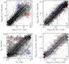 |
Fig. 10. Same as Fig. 9, but using a CNN that was trained on mock clusters with simulated uncertainty of photometric calibrations. |
Figure 11 shows the derived classc/b and visibility values for the 5000 test mock clusters and for a random sample of 5000 M 83 background images. As can be seen in the histogram on top, the classc/b parameter is predicted as > 0.5 for the vast majority of mock cluster images, and as < 0.5 for the majority of background images. This suggests that the fraction of background images that are classified as classc/b > 0.5 are likely to correspond to real clusters. The visibility parameter is highly correlated with classc/b, again showing high values for the majority of mock clusters and low values for the majority of backgrounds. The few remaining mock clusters with classc/b < 0.5 have very low visibility values, which indicates faint, nearly invisible objects seen in Fig. 4.
 |
Fig. 11. Visibility parameter values vs. classc/b for mock (red) and random M 83 field (gray) samples. The histograms are marginalized logarithmic counts of samples for visibility (right) and classc/b (top). Top right panel: true vs. derived visibility parameters of mock clusters as a logarithmic density map; dashed lines outline the area containing 95% of the clusters. |
Figure 12 illustrates selection effects by showing the derived age, extinction, mass, and size parameters of the test mock clusters; the color bar represents the derived visibility parameter value for each cluster. In Fig. 12a it can be seen that mass and age are correlated as expected when deriving the visibility parameter: clusters with lower mass and older ages tend to be less visible (this can also be seen in Figs. 1 and 2). The same is true for extinction (panels b and d), as higher extinctions tend to make cluster less visible, and size (panels c, d, and f), as more concentrated clusters stand out relative to their backgrounds.
 |
Fig. 12. Inferred parameter distributions for the test cluster sample. The panels show the following parameter combinations: (a) mass vs. age, (b) extinction vs. age, (c) size vs. age, (d) extinction vs. mass, (e) size vs. mass, and (f) size vs. extinction. Diagonal cutoffs in panels (a) and (b) are related to the cluster detection limit, applied as magnitude cuts, shown in Fig. 3. The color map represents the visibility parameter, which acts as a proxy for the selection effects in a magnitude limited sample, while also taking into account variable cluster sizes and extinctions. |
Even though the cluster-related parameter inference results for background images have no inherit meaning, the CNN produces values for all of its output neurons regardless. Looking at these values can provide us with additional insights. For example, we would expect backgrounds to be classified as low-mass extended objects. Figure 13 shows the derived parameters for the background images from Fig. 11; dot size and color indicate classc/b. The black dots represent images with classc/b close to 0, while the red circles indicate images with classc/b close to 1. As can be seen in Fig. 13e, the vast majority of the backgrounds are classified as low-mass extended objects as expected; some probable cluster images are spread out more evenly through the parameter space. The derived age values of these images are spread out through the whole age range (panels a, b, and c), however extinctions are heavily correlated with ages as seen in panel b. As the network is trained to predict extinction and age values regardless of what the background of the cluster looks like, there is no intuitive value that should be predicted for background images in this case. In effect the CNN avoids areas of age-extinction parameter space where the appearance of an observed object is either extremely blue (high-extinction high-age) or extremely red (low-extinction low-age), which can only be associated with genuine clusters, resulting in this diagonal effect.
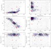 |
Fig. 13. Same as in Fig. 12, but for 5000 randomly spatially sampled M 83 background images. For reference, derived mock cluster parameters are shown as faint gray dots. Real background samples are shown as black dots, which transition to blue and then to red. The dot size and color represents classc/b. The blue dots indicate objects with classc/b > 0.5 and the red dots indicate objects with classc/b > 0.99. |
The classc/b parameter was shown to be usable in differentiating between cluster and background images, while the visibility parameter is correlated well with those cluster parameter ranges, which can show more confidently identified clusters. We conclude that these parameters can be useful indicators in star cluster search application.
4.2. Validation with cataloged clusters
To validate our method on real clusters, we used three previous M 83 HST star cluster studies that had published catalogs. This includes the study covering the whole galactic disk (7 WFC3 fields) by Ryon et al. (2015, R15), two WFC3 fields by Bastian et al. (2011, B11) and the central region of the galaxy by Harris et al. (2001, H01).
The study by Bastian et al. (2011) is comprised of 939 objects. We discarded objects with missing parameter values, leaving us with 889 of them to compare to the CNN inference results. Bastian et al. (2011) estimate the cluster age, mass, and extinction by comparing the integral photometry of the observed clusters to SSP models. Meanwhile, the sizes of clusters were estimated by fitting spatial models to F438W, F555W, and F814W band images. For this comparison we took the median value of these three size estimates. As the cluster magnitudes used by Bastian et al. (2011) are Galactic extinction corrected, we shift the AV values of those objects by 0.3 mag6. This allows us to compare CNN derived values directly because we compute total extinctions for clusters regardless of the dust source.
Figures 14 and 15 show a comparison between Bastian et al. (2011) and CNN-derived values. In Fig. 14 the red and blue dots represent clusters with significantly overestimated and underestimated extinction values, respectively. They were defined as clusters that are outside the dashed lines in panel c, which represent the area containing 95% of mock cluster parameter derivations. This mirrors the situation with mock objects in Fig. 9, as the majority of clusters with overestimated extinctions end up with underestimated ages, and vice versa for clusters with underestimated extinction values. These effects can again be attributed to the age-extinction degeneracy. In Fig. 15 the green dots represent images classified by the network as likely to be real clusters (classc/b ≥ 0.5), while the magenta dots are objects with classc/b < 0.5. The vast majority of the objects are classified as likely clusters.
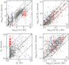 |
Fig. 14. Comparisons for (a) age, (b) mass, (c) AV, and (d) rh derived by Bastian et al. (2011) and by CNN. The red dots represent clusters with overestimated, while the blue dots represent clusters with underestimated extinction values with respect to Bastian et al. (2011). The remaining clusters are shown in gray. The dashed lines outline the area containing 95% of the mock clusters. |
 |
Fig. 15. Same as Fig. 14, but with large green dots representing objects classified as likely clusters (classc/b ≥ 0.5), and magenta dots representing objects with classc/b < 0.5. Mock clusters are shown in the background as a hexagonal density maps with bins scaled linearly. |
Overall the derived ages and masses show a reasonable correlation between Bastian et al. (2011) and CNN-derived values. Many of the objects have cataloged AV = 0 mag values (shown as AV = 0.3 mag in the figures, accounting for Galactic extinction). The CNN derives higher extinctions for some of these clusters, however, visual inspection has revealed that Galactic dust is unlikely to be the only source of extinction for the majority of them. The sizes show a good agreement for most of the objects, however, there is a subset of objects with somewhat overestimated values.
For the comparison with Ryon et al. (2015) we used 478 objects that had sizes obtained by a 2D spatial model fitting along with age and mass estimates derived using spectral energy distribution fitting. We also took 45 objects from Harris et al. (2001) whose age, mass, and extinction estimates were obtained by comparing the cluster photometry to theoretical population synthesis models. Figure 16 shows our results compared against both of these catalogs. Ryon et al. (2015) objects are denoted as green dots with the parameter error bounds indicated with black lines. Harris et al. (2001) objects are indicated as large cyan circles. For both of these catalogs a reasonable agreement with the CNN-derived values can be seen; only masses are slightly overestimated. However, there is some age estimate divergence over log10(t/yr) = 8, which is similar to the situation in Fig. 14.
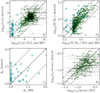 |
Fig. 16. Same as Fig. 15, but with green dots representing objects from Ryon et al. (2015) and cyan dots representing objects from Harris et al. (2001). The horizontal bars denote minimum and maximum parameter values for age and mass, and statistical errors for size, as provided in the catalogs. |
We have shown that the CNN is capable of deriving cluster parameters on real clusters by comparing our results with those of other authors. The agreements between the values are reasonable and follow the results obtained with mock clusters. However, owing to the age-extinction degeneracy with the three passbands used, the results with clusters older than log10(t/yr) = 8 are ambiguous and should be interpreted carefully.
5. Discussion
We have shown the applicability of a CNN-based method in deriving a variety of star cluster parameters from M 83 mosaic images in terms of quantitative error analysis. However, the final aim for this method is to be of use in star cluster search and automatic catalog construction. To this end, a better look into the derived parameters is needed both in terms of each other and their context in the galaxy. In this chapter we look at derived values of the Bastian et al. (2011) sample of objects in more detail.
Figure 17 shows the inferred age, extinction, mass, and size parameters of the Bastian et al. (2011) object sample. The objects are colored as in Fig. 15, in which mock results are shown in the background. The clusters cover the whole parameter range well; classc/b < 0.5 samples are classified as low-mass objects (panel a), as expected. The minimal extinction line, with a large number of clusters around it, seen in panels b, d, and f, coincides with AV ∼ 0.3 mag, expected due to Galactic dust foreground in the direction of M 83. Lines of constant density are shown in panel e. The majority of the objects fall within 10 and 103 M⊙/pc−3, which is consistent with results for clusters of the M 31 galaxy (Vansevičius et al. 2009).
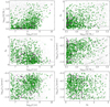 |
Fig. 17. Same as Fig. 12, but for objects from Bastian et al. (2011), with values derived by CNN. The green circles represent objects classified as likely clusters, while magenta circles represent likely non-clusters, as in Fig. 15. For reference, the derived parameters of the mock cluster set are shown as faint gray points. Panel e: locations of clusters with the same density, varying from 10 to 104 M⊙/pc−3. In panels b, d, and f the solid black lines represent the amount of Galactic extinction in the direction of M 83 (AV = 0.3 mag). |
Figure 18 shows Bastian et al. (2011) objects denoted on two fields of the M 83 mosaic. Objects of log10(t/yr) < 7.4 are indicated as blue circles in panel a, log10(t/yr) < 8.6 objects are denoted as orange circles in panel b, and log10(t/yr) ≥ 8.6 objects are denoted as red circles in panel c. Panel d shows all of the objects marked as dots, with AV < 1 mag colored cyan, and AV ≥ 1 mag colored magenta. The spatial distribution of objects is sensible, wherein young star clusters are grouped around the galaxies spiral arms, near the dust clouds where they were formed, and old clusters are spread out more evenly throughout the galaxy, as they had more time to drift away. The extinction distributions are less clear cut, however some crowding around dust-heavy regions can be seen by the high-extinction objects, as is expected. The spatial distributions of age-selected clusters in Fig. 18 correspond well to the results obtained by Fouesneau et al. (2012) using UBVIHα fluxes to measure ages, masses, and extinctions in the central region of M 83. Sánchez-Gil et al. (2019) derive age maps for the M 83 galaxy’s stellar populations younger than 20 Myr, which corresponds to the lower age range of clusters in this study.
 |
Fig. 18. M 83 mozaic of the F438W passband observations, overplotted with young – log10(t/yr) < 7.4 (blue), intermediate – 7.4 ≤ log10(t/yr) < 8.6 (yellow), and old – log10(t/yr) ≥ 8.6 (red) objects from Bastian et al. (2011). Last panel: objects with low – AV < 1 mag (cyan) and high – AV ≥ 1 mag (magenta) extinctions. |
Although we studied clusters with masses log(M/M⊙) = [3.5, 5.5], this does not imply that only such clusters are detectable with the HST/WFC3 observations of M 83. Clusters with masses as low as log(M/M⊙)∼3 have been studied by Whitmore et al. (2011) and Andrews et al. (2014). However, such clusters are dominated by stochastic effects of IMF sampling making the analysis of the effects of extinction problematic. The lower limit of masses was selected to focus on the effects of extinction and to align with the range of clusters used by Bastian et al. (2011). The presented CNN classifies lower mass clusters as being on the lower limit of this range.
Figure 19 shows the binned mass distributions obtained with the CNN. The gray outline shows all of the cluster distributions; the blue dots represent clusters of log10(t/yr) < 7.7 (panel a) and 7.7 ≤ log10(t/yr) < 8.7 (panel b). The red lines represent Schechter type mass functions (Portegies Zwart et al. 2010) with various amounts of truncation. The solid red line follows the non-truncated power-law dN/dM = A ⋅ M−2, the dashed red line follows  , and the dotted red line follows
  . The power-law distributions fit the data well for both of the age cuts, however, there is a lack of low-mass clusters (log10(M/M⊙) ≤ 4) for the mid-age data sample. This is due to selection effects, where less star clusters are detectable at those ages (see Fig. 17a). Similar cluster mass distributions and selection effects are found in M 31 (Vansevičius et al. 2009) and M 33 (de Meulenaer et al. 2015) star cluster samples.
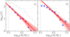 |
Fig. 19. Cluster mass distributions for samples with ages log10(t/yr) < 7.7 (a) and 7.7 < log10(t/yr) < 8.7 (b). The lines represent the power-law mass distribution function of the form dN/dM = A ⋅ M−2 ⋅ exp(−M/M*): M* = ∞ (solid line, with the shaded area encompassing its Poisson standard deviation), 106 M⊙ (dashed line), and 2.5 × 10⁵ M⊙ (dotted line). |
Figure 20 show examples of inference results on three distinct Bastian et al. (2011) clusters chosen to illustrate the variety of CNN outputs (previously sketched in Fig. 6). The top row shows a young, low-mass cluster. The inferred age and mass matches Bastian et al. (2011) parameters well. Extinction is derived to be slightly higher, however the value is very close when Galactic extinction is accounted for. The visibility parameter is derived to be ∼15, which corresponds well to similarly looking clusters in Fig. 2b.
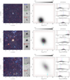 |
Fig. 20. Examples of real clusters and their parameter distributions inferred by the CNN. Left panels: color image of each cluster in a field of 7″ × 7″, with a 2.6″ × 2.6″ field used for inference highlighted with a dashed square. The three grayscale images are represented as the three passband observations shown separately. All of the images are normalized as in Fig. 1. The remaining panels depict inference results; the histograms show the neuron activations of the neural network for the given parameter. Age and extinction is depicted as a 2D activation map marginalized over mass to highlight the effects of age-extinction degeneracies; the color bar on the top indicates CNN output neuron activation strength. The Bastian et al. (2011) derived values of parameters are denoted in cyan, and the CNN inferred values in magenta. The light red shaded areas show parameter ranges in which the CNN produces activations, but were not covered by the clusters used in this study to deal with parameter boundary effects. The empty cyan circle in the age-extinction map represents the values obtained after Galactic extinction correction. |
In the middle, a cluster of log10(t/yr)∼8.3, medium extinction and high mass is shown. The age, mass, and size correspond well to the values derived by Bastian et al. (2011). Extinction is derived as slightly higher, however it is still within the range of the activations. The cluster is classified as brighter by the CNN, with visibility ∼ 25.
On the bottom an older cluster is depicted. Its mass and size estimates correspond well, however extinction is overestimated in comparison to Bastian et al. (2011). Furthermore, the neuron activations show a diagonal pattern highlighting the age-extinction degeneracy, which is hard to resolve with the used three passbands. However, the higher extinction results are more likely as a significant amount of the field seen in the leftmost panel appears reddened, which suggest the presence of dust obscuring the cluster.
As detailed in Sect. 3.3, a correlation between the spread of CNN output activations and scatter of inferred cluster parameters is noted, therefore, activation maps can be used to estimate cluster parameter uncertainties. We checked that less than 1% of the clusters show the bimodal distribution activation distributions and about 20% of the samples show an extended unimodal distribution (see Fig. 8 for examples). The rest of the results are unimodal. Therefore, selecting the highest activation and interpolating it is a viable approach to provide inferred parameter estimates. However, there are some cases in which there is a systematic bias in the derived results. This usually occurs for the nearly invisible clusters as well as clusters with high extinctions and older ages, where age-extinction degeneracies make inference unreliable with the photometric passbands used. This means that the extent of activation maps alone, while informative, is not a reliable uncertainty estimate in all cases. Additional insights on the reliability of inference results can be gained by performing the random background sampling test described in Sect. 3.3.
These results further validate the applicability of the CNN in deriving the parameters of star clusters in realistic scenarios. In addition, the classc/b and visibility parameters act as accurate proxies for cluster presence in images. Utilizing this method for constructing a full catalog of M 83 clusters is left for the subsequent paper in the series.
6. Conclusions
We have extended the method introduced in Paper I to infer cluster ages, masses, sizes, extinctions, and to account for the degeneracies between these parameters. Additional parameters were added to identify the presence of clusters on background images of M 83 and to judge their visibility (S/N).
To train this network a bank of mock clusters was generated utilizing three photometric passbands in the context of the M 83 galaxy. The CNN was verified on mock images of artificial clusters with ages, log10(t/yr), between 6.6 and 10.1, masses, log10(M/M⊙), between 3.5 and 5.5, sizes between 0.04 and 0.4 arcsec, and extinctions AV ≤ 3 mag. Parameters derived by CNN have shown a good agreement with the true parameters for log10(t/yr) < 8, where higher age estimates are unreliable because of the age-extinction degeneracy. Real cluster parameter inference tests were performed with three different M 83 cluster catalogs from Bastian et al. (2011), Ryon et al. (2015), and Harris et al. (2001) and have shown consistent results.
We demonstrated that a CNN can perform evolutionary (age, mass), structural (size), and environmental (extinction) star cluster parameter inference. In addition, the network is capable of giving an indication of cluster presence in images. Therefore, the created CNN is a useful tool for further research in constructing a full pipeline of star cluster detection and parameter inference.
Acknowledgments
This research was funded by a grant (No. LAT-09/2016) from the Research Council of Lithuania. This research made use of Astropy, a community-developed core Python package for Astronomy (Astropy Collaboration 2018). Some of the data presented in this paper were obtained from the Mikulski Archive for Space Telescopes (MAST). STScI is operated by the Association of Universities for Research in Astronomy, Inc., under NASA contract NAS5-26555. We are thankful to the anonymous referee who helped improve the paper.
References
- Andrews, J. E., Calzetti, D., Chandar, R., et al. 2014, ApJ, 793, 4 [NASA ADS] [CrossRef] [Google Scholar]
- Astropy Collaboration (Price-Whelan, A. M., et al.) 2018, AJ, 156, 123 [Google Scholar]
- Bastian, N., Adamo, A., Gieles, M., et al. 2011, MNRAS, 417, L6 [NASA ADS] [Google Scholar]
- Bialopetravičius, J., Narbutis, D., & Vansevičius, V. 2019, A&A, 621, A103 [NASA ADS] [CrossRef] [EDP Sciences] [Google Scholar]
- Blair, W. P., Chandar, R., Dopita, M. A., et al. 2014, ApJ, 788, 55 [NASA ADS] [CrossRef] [Google Scholar]
- Bressan, A., Marigo, P., Girardi, L., et al. 2012, MNRAS, 427, 127 [NASA ADS] [CrossRef] [Google Scholar]
- Bridžius, A., Narbutis, D., Stonkutė, R., Deveikis, V., & Vansevičius, V. 2008, Balt. Astron., 17, 337 [NASA ADS] [Google Scholar]
- de Meulenaer, P., Narbutis, D., Mineikis, T., & Vansevičius, V. 2013, A&A, 550, A20 [NASA ADS] [CrossRef] [EDP Sciences] [Google Scholar]
- de Meulenaer, P., Narbutis, D., Mineikis, T., & Vansevičius, V. 2014, A&A, 569, A4 [NASA ADS] [CrossRef] [EDP Sciences] [Google Scholar]
- de Meulenaer, P., Narbutis, D., Mineikis, T., & Vansevičius, V. 2015, A&A, 581, A111 [NASA ADS] [CrossRef] [EDP Sciences] [Google Scholar]
- Dieleman, S., Willett, K. W., & Dambre, J. 2015, MNRAS, 450, 1441 [NASA ADS] [CrossRef] [Google Scholar]
- Dopita, M. A., Blair, W. P., Long, K. S., et al. 2010, ApJ, 710, 964 [NASA ADS] [CrossRef] [Google Scholar]
- Dressel, L. 2012, Wide Field Camera 3 Instrument Handbook for Cycle 21 v. 5.0 [Google Scholar]
- Elson, R. A. W., Fall, S. M., & Freeman, K. C. 1987, ApJ, 323, 54 [NASA ADS] [CrossRef] [Google Scholar]
- Fouesneau, M., & Lançon, A. 2010, A&A, 521, A22 [NASA ADS] [CrossRef] [EDP Sciences] [Google Scholar]
- Fouesneau, M., Lançon, A., Chandar, R., & Whitmore, B. C. 2012, ApJ, 750, 60 [NASA ADS] [CrossRef] [Google Scholar]
- Harris, J. D., Calzetti, III., J. S. G., Conselice, C. J., & Smith, D. A. 2001, AJ, 122, 3046 [NASA ADS] [CrossRef] [Google Scholar]
- He, K., Zhang, X., Ren, S., & Sun, J. 2016, 2016 IEEE Conference on Computer Vision and Pattern Recognition (CVPR), 770 [Google Scholar]
- Hernandez, S., Larsen, S., Aloisi, A., et al. 2019, ApJ, 872, 116 [NASA ADS] [CrossRef] [Google Scholar]
- Kingma, D. P., & Ba, J. 2014, ArXiv e-prints [arXiv:1412.6980] [Google Scholar]
- Krist, J. E., Hook, R. N., & Stoehr, F. 2011, in Optical Modeling and Performance Predictions V, Proc. SPIE, 8127, 81270J [Google Scholar]
- Kroupa, P. 2001, MNRAS, 322, 231 [NASA ADS] [CrossRef] [Google Scholar]
- Krumholz, M. R., Fumagalli, M., da Silva, R. L., Rendahl, T., & Parra, J. 2015, MNRAS, 452, 1447 [NASA ADS] [CrossRef] [Google Scholar]
- McConnachie, A. W., Irwin, M. J., Ferguson, A. M. N., et al. 2005, MNRAS, 356, 979 [NASA ADS] [CrossRef] [Google Scholar]
- Portegies Zwart, S. F., McMillan, S. L. W., & Gieles, M. 2010, ARA&A, 48, 431 [NASA ADS] [CrossRef] [Google Scholar]
- Reyes, E., Estévez, P. A., Reyes, I., et al. 2018, 2018 International Joint Conference on Neural Networks (IJCNN), 1 [Google Scholar]
- Ribli, D., Dobos, L., & Csabai, I. 2019, MNRAS, 489, 4847 [NASA ADS] [CrossRef] [Google Scholar]
- Rowe, B. T. P., Jarvis, M., Mandelbaum, R., et al. 2015, Astron. Comput., 10, 121 [NASA ADS] [CrossRef] [Google Scholar]
- Russakovsky, O., Deng, J., Su, H., et al. 2015, Int. J. Comput. Vision, 115, 211 [Google Scholar]
- Ryon, J. E., Bastian, N., Adamo, A., et al. 2015, MNRAS, 452, 525 [NASA ADS] [CrossRef] [Google Scholar]
- Sánchez-Gil, M. C., Alfaro, E. J., Cerviño, M., et al. 2019, MNRAS, 483, 2641 [NASA ADS] [CrossRef] [Google Scholar]
- Thim, F., Tammann, G. A., Saha, A., et al. 2003, ApJ, 590, 256 [NASA ADS] [CrossRef] [Google Scholar]
- Vansevičius, V., Kodaira, K., Narbutis, D., et al. 2009, ApJ, 703, 1872 [NASA ADS] [CrossRef] [Google Scholar]
- Whitmore, B. C., Chandar, R., Kim, H., et al. 2011, ApJ, 729, 78 [NASA ADS] [CrossRef] [Google Scholar]
- Wu, C., Wong, O. I., Rudnick, L., et al. 2019, MNRAS, 482, 1211 [NASA ADS] [CrossRef] [Google Scholar]
All Tables
All Figures
|
Fig. 1. Examples of generated mock clusters placed on a real background image, which is the same for all panels. The ages of the clusters are shown top of each panel. The mass and size, rh, values are varied as shown on the axes; extinction AV = 0 mag. The intensity scale of the images was normalized with the arcsinh function within identical pixel value limits for each image. The yellow circles represent rh, obs values (rh convolved with the PSF). The value of the visibility, i.e., S/N proxy, is shown on the bottom left of each image for fainter objects with visibility < 100. Image sizes are 64 × 64 pixels (2.6 × 2.6 arcsec) or ∼60 × 60 pc at the distance of M 83. In the images red corresponds to passband F814W, green to F438W, and blue to F336W. |
| In the text | |
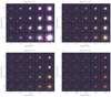 |
Fig. 2. Same as Fig. 1, but with AV = 1 mag. |
| In the text | |
|
Fig. 3. Integrated color-color and color-magnitude diagrams of 50 000 generated mock clusters of the training bank and ∼7000 faint clusters. The color coding represents different ages (a, e), extinctions (b, f), and masses (c, g). Their values are as noted on the color bars on top. The last column (d, h) shows distributions of AV < 0.2 mag star clusters filtered by three mass ranges as specified on the color bar on top. The SSP tracks centered on the specified masses are shown as black curves. The shaded area below the dashed line represents the F814W magnitude limit used to filter out faint clusters. |
| In the text | |
|
Fig. 4. Examples of generated mock clusters with varying ages and extinctions on real background images. The masses of the clusters are log10(M/M⊙) = 4.5, their sizes are log 10(rh/arcsec) = −0.7. The images are normalized as in Fig. 1. Top panel: clusters superimposed on a sparse background, bottom panel: same clusters superimposed on a denser background. The visibility value is indicated on the bottom left of each image. The sizes of the images are 64 × 64 pix. |
| In the text | |
|
Fig. 5. Block diagram of the CNN. The three-channel input image of a cluster passes through the network top to bottom; the output result are age, extinction, mass, size, the cluster-background class classc/b, and visibility. All blocks with sharp corners depict single layers, while blocks with rounded corners are groupings of layers. The number on the left indicates how many times the group is repeated sequentially and the name on the right corresponds to the layer names in Table 1. The blocks with non-white backgrounds are parts of the network with optimizable parameters. The last number in each row is the number of output channels from that layer. “ReLU” indicates the locations in the network where rectified linear activations are applied between blocks. |
| In the text | |
|
Fig. 6. Illustration of the activations in the output layers of the CNN. While training the CNN, target activation values are provided as a 3D Gaussian distribution for age, extinction, and mass (centered on true values as denoted by the red dot) and as 1D Gaussian distributions for rh (the blue line) and visibility (the red line). classc/b is represented as a value of 0 or 1. During inference the network produces similar outputs, examples of which are depicted in Figs. 8 and 20. |
| In the text | |
|
Fig. 7. Binary classification accuracy metric for classc/b on the training (orange) and validation (blue) sets during the course of CNN training. |
| In the text | |
|
Fig. 8. Influence of stochastic effects on mock cluster inference results. Left column: clusters with log10(M/M⊙) = 5.0 and varied extinction and age. Right column: clusters with AV = 0.5 mag and varied mass and age. Cluster sizes are fixed at log10(rh/arcsec) = −0.6 for all cases. Top row: results of inference when stellar IMF sampling and spatial positions are varied while holding the cluster parameters constant. Middle row: results of inference when background images are varied while using the same cluster image. The cyan circles correspond to the true values of parameters. The grayscale colormaps are raw CNN outputs (activations over the parameter space) for one specific mock cluster case, while magenta circles show 100 single-point estimates obtained for different random cases. Bottom row: visualizations of the clusters with fixed background in the same format as in Fig. 4. |
| In the text | |
|
Fig. 9. True and derived parameter values of test mock clusters visualized as a hexagonal density map. The bins are scaled logarithmically. Panels show comparisons for (a) age, (b) mass, (c) AV, and (d) rh. The dashed lines highlight the area containing 95% of the clusters. The red dots represent the clusters that were misclassified as younger than the real age values, while the blue dots represent clusters misclassified as older. |
| In the text | |
|
Fig. 10. Same as Fig. 9, but using a CNN that was trained on mock clusters with simulated uncertainty of photometric calibrations. |
| In the text | |
|
Fig. 11. Visibility parameter values vs. classc/b for mock (red) and random M 83 field (gray) samples. The histograms are marginalized logarithmic counts of samples for visibility (right) and classc/b (top). Top right panel: true vs. derived visibility parameters of mock clusters as a logarithmic density map; dashed lines outline the area containing 95% of the clusters. |
| In the text | |
|
Fig. 12. Inferred parameter distributions for the test cluster sample. The panels show the following parameter combinations: (a) mass vs. age, (b) extinction vs. age, (c) size vs. age, (d) extinction vs. mass, (e) size vs. mass, and (f) size vs. extinction. Diagonal cutoffs in panels (a) and (b) are related to the cluster detection limit, applied as magnitude cuts, shown in Fig. 3. The color map represents the visibility parameter, which acts as a proxy for the selection effects in a magnitude limited sample, while also taking into account variable cluster sizes and extinctions. |
| In the text | |
|
Fig. 13. Same as in Fig. 12, but for 5000 randomly spatially sampled M 83 background images. For reference, derived mock cluster parameters are shown as faint gray dots. Real background samples are shown as black dots, which transition to blue and then to red. The dot size and color represents classc/b. The blue dots indicate objects with classc/b > 0.5 and the red dots indicate objects with classc/b > 0.99. |
| In the text | |
|
Fig. 14. Comparisons for (a) age, (b) mass, (c) AV, and (d) rh derived by Bastian et al. (2011) and by CNN. The red dots represent clusters with overestimated, while the blue dots represent clusters with underestimated extinction values with respect to Bastian et al. (2011). The remaining clusters are shown in gray. The dashed lines outline the area containing 95% of the mock clusters. |
| In the text | |
|
Fig. 15. Same as Fig. 14, but with large green dots representing objects classified as likely clusters (classc/b ≥ 0.5), and magenta dots representing objects with classc/b < 0.5. Mock clusters are shown in the background as a hexagonal density maps with bins scaled linearly. |
| In the text | |
|
Fig. 16. Same as Fig. 15, but with green dots representing objects from Ryon et al. (2015) and cyan dots representing objects from Harris et al. (2001). The horizontal bars denote minimum and maximum parameter values for age and mass, and statistical errors for size, as provided in the catalogs. |
| In the text | |
|
Fig. 17. Same as Fig. 12, but for objects from Bastian et al. (2011), with values derived by CNN. The green circles represent objects classified as likely clusters, while magenta circles represent likely non-clusters, as in Fig. 15. For reference, the derived parameters of the mock cluster set are shown as faint gray points. Panel e: locations of clusters with the same density, varying from 10 to 104 M⊙/pc−3. In panels b, d, and f the solid black lines represent the amount of Galactic extinction in the direction of M 83 (AV = 0.3 mag). |
| In the text | |
|
Fig. 18. M 83 mozaic of the F438W passband observations, overplotted with young – log10(t/yr) < 7.4 (blue), intermediate – 7.4 ≤ log10(t/yr) < 8.6 (yellow), and old – log10(t/yr) ≥ 8.6 (red) objects from Bastian et al. (2011). Last panel: objects with low – AV < 1 mag (cyan) and high – AV ≥ 1 mag (magenta) extinctions. |
| In the text | |
|
Fig. 19. Cluster mass distributions for samples with ages log10(t/yr) < 7.7 (a) and 7.7 < log10(t/yr) < 8.7 (b). The lines represent the power-law mass distribution function of the form dN/dM = A ⋅ M−2 ⋅ exp(−M/M*): M* = ∞ (solid line, with the shaded area encompassing its Poisson standard deviation), 106 M⊙ (dashed line), and 2.5 × 10⁵ M⊙ (dotted line). |
| In the text | |
|
Fig. 20. Examples of real clusters and their parameter distributions inferred by the CNN. Left panels: color image of each cluster in a field of 7″ × 7″, with a 2.6″ × 2.6″ field used for inference highlighted with a dashed square. The three grayscale images are represented as the three passband observations shown separately. All of the images are normalized as in Fig. 1. The remaining panels depict inference results; the histograms show the neuron activations of the neural network for the given parameter. Age and extinction is depicted as a 2D activation map marginalized over mass to highlight the effects of age-extinction degeneracies; the color bar on the top indicates CNN output neuron activation strength. The Bastian et al. (2011) derived values of parameters are denoted in cyan, and the CNN inferred values in magenta. The light red shaded areas show parameter ranges in which the CNN produces activations, but were not covered by the clusters used in this study to deal with parameter boundary effects. The empty cyan circle in the age-extinction map represents the values obtained after Galactic extinction correction. |
| In the text | |
Current usage metrics show cumulative count of Article Views (full-text article views including HTML views, PDF and ePub downloads, according to the available data) and Abstracts Views on Vision4Press platform.
Data correspond to usage on the plateform after 2015. The current usage metrics is available 48-96 hours after online publication and is updated daily on week days.
Initial download of the metrics may take a while.