Photometric detection of internal gravity waves in upper main-sequence stars

D. M. Bowman; C. Aerts; C. Johnston; M. G. Pedersen; T. M. Rogers; P. V. F. Edelmann; S. Simón-Díaz; T. Van Reeth; B. Buysschaert; A. Tkachenko; S. A. Triana

doi:10.1051/0004-6361/201833662

Home

All issues

Volume 621 (January 2019)

A&A, 621 (2019) A135

Full HTML

Free Access

Issue		A&A Volume 621, January 2019


Article Number		A135
Number of page(s)		41
Section		Stellar structure and evolution
DOI		https://doi.org/10.1051/0004-6361/201833662
Published online		21 January 2019

A&A 621, A135 (2019)

I. Methodology and application to CoRoT targets

D. M. Bowman¹, C. Aerts¹^,2, C. Johnston¹, M. G. Pedersen¹, T. M. Rogers³^,4, P. V. F. Edelmann³, S. Simón-Díaz⁵^,6, T. Van Reeth⁷^,8, B. Buysschaert¹^,9, A. Tkachenko¹ and S. A. Triana¹⁰

¹ Instituut voor Sterrenkunde, KU Leuven, Celestijnenlaan 200D, 3001 Leuven, Belgium
e-mail: dominic.bowman@kuleuven.be
² Department of Astrophysics, IMAPP, Radboud University Nijmegen, 6500 GL Nijmegen, The Netherlands
³ School of Mathematics, Statistics and Physics, Newcastle University, Newcastle-upon-Tyne NE1 7RU, UK
⁴ Planetary Science Institute, Tucson, AZ 85721, USA
⁵ Instituto de Astrofísica de Canarias, 38200 La Laguna, Tenerife, Spain
⁶ Departamento de Astrofísica, Universidad de La Laguna, 38205 La Laguna, Tenerife, Spain
⁷ Sydney Institute for Astronomy (SIfA), School of Physics, The University of Sydney, NSW 2006, Australia
⁸ Stellar Astrophysics Centre, Department of Physics and Astronomy, Aarhus University, Ny Munkegade 120, 8000 Aarhus C, Denmark
⁹ LESIA, Observatoire de Paris, PSL Research University, CNRS, Sorbonne Universités, UPMC Univ. Paris 06, Univ. Paris Diderot, Sorbonne Paris Cité, 5 Place Jules Janssen, 92195 Meudon, France
¹⁰ Royal Observatory of Belgium, Ringlaan 3, 1180 Brussels, Belgium

Received: 17 June 2018
Accepted: 16 November 2018

Abstract

Context. Main sequence stars with a convective core are predicted to stochastically excite internal gravity waves (IGWs), which effectively transport angular momentum throughout the stellar interior and explain the observed near-uniform interior rotation rates of intermediate-mass stars. However, there are few detections of IGWs, and fewer still made using photometry, with more detections needed to constrain numerical simulations.

Aims. We aim to formalise the detection and characterisation of IGWs in photometric observations of stars born with convective cores (M ≳ 1.5 M_⊙) and parameterise the low-frequency power excess caused by IGWs.

Methods. Using the most recent CoRoT light curves for a sample of O, B, A and F stars, we parameterised the morphology of the flux contribution of IGWs in Fourier space using an MCMC numerical scheme within a Bayesian framework. We compared this to predictions from IGW numerical simulations and investigated how the observed morphology changes as a function of stellar parameters.

Results. We demonstrate that a common morphology for the low-frequency power excess is observed in early-type stars observed by CoRoT. Our study shows that a background frequency-dependent source of astrophysical signal is common, which we interpret as IGWs. We provide constraints on the amplitudes of IGWs and the shape of their detected frequency spectrum across a range of mass, which is the first ensemble study of stochastic variability in such a diverse sample of stars.

Conclusions. The evidence of a low-frequency power excess across a wide mass range supports the interpretation of IGWs in photometry of O, B, A and F stars. We also discuss the prospects of observing hundreds of massive stars with the Transiting Exoplanet Survey Satellite (TESS) in the near future.

Key words: asteroseismology / stars: early-type / stars: oscillations / stars: evolution / stars: rotation

© ESO 2019

1. Introduction

Understanding the physics at work within massive stars is a significant goal for astronomy as these stars are dominant in stellar and galactic evolution theory (Maeder & Meynet 2000). Specifically, the radial rotation profile, interior mixing and angular momentum transport mechanisms are poorly constrained, yet they dramatically influence stellar structure and evolution theory (Zahn 1992; Heger et al. 2000; Maeder 2009; Meynet et al. 2013; Aerts et al. 2018b). Only detailed observational constraints of stellar interiors provide the ability to mitigate uncertainties in current stellar models (e.g. Aerts et al. 2017b; Ouazzani et al. 2018).

Asteroseismology is a vastly successful method for directly probing the interior structure and physical processes occurring within a star. This methodology uses surface variability caused by stellar oscillations generated within a star’s interior to probe the physics at work at different depths, with a detailed monograph provided by Aerts et al. (2010). Stellar oscillations are governed by the physics of driving and damping. Some driving mechanisms produce standing waves (i.e. coherent pulsation modes) with characteristic frequencies and long mode lifetimes. Pressure (p) modes are sound waves, for which pressure is the dominant restoring force and are most sensitive to the surface layers within a star (Aerts et al. 2010). Whereas gravity (g) modes have buoyancy as the dominant restoring force and are most sensitive to the near-core region. For practically all stars, rotation and specifically the Coriolis force also act as a restoring force. When the Coriolis force is the dominant restoring force, one also gets inertial modes (also known as r modes). In the case of gravito-inertial pulsation modes, both buoyancy and the Coriolis force are important.

The research field of asteroseismology has greatly and rapidly expanded in the last decade because of high-precision and high duty-cycle photometric data sets from space missions such as CoRoT (Auvergne et al. 2009), Kepler (Borucki et al. 2010) and K2 (Howell et al. 2014). These telescopes began a space photometry revolution and provided the first truly high-quality asteroseismic data sets, which have photometric precisions that are hundreds of times better than achievable from the ground. Furthermore, these data sets were amongst the first continuous data sets long enough to provide the high frequency resolution required for detailed asteroseismic studies of different types of pulsating stars. Of course, ground-based multi-site campaigns can offer long-term monitoring of pulsating stars, but typically have lower duty cycles, much higher noise levels and are subject to aliasing problems (see e.g. Breger 2000; Breger et al. 2002, 2004; Kurtz et al. 2005; Bowman et al. 2015), which can make identification of individual pulsation modes difficult.

The 4-yr Kepler mission data have proven particularly useful for studying the interior properties of intermediate-mass stars (Aerts et al. 2017b). To date, approximately 70 main-sequence B, A and F stars have been measured to have near-uniform radial rotation rates (Degroote et al. 2010a; Kurtz et al. 2014; Pápics et al. 2014, 2017; Saio et al. 2015; Van Reeth et al. 2015, 2018; Triana et al. 2015; Murphy et al. 2016; Ouazzani et al. 2017, 2018; Zwintz et al. 2017). However, more observational studies of intermediate- and especially high-mass stars are needed to address the large shortcomings in the theory of angular momentum transport when comparing observations of main sequence and evolved stars (Tayar & Pinsonneault 2013; Cantiello et al. 2014; Eggenberger et al. 2017; Aerts et al. 2017b, 2018b; Ouazzani et al. 2018). To produce a near-uniform rotation rate within a star during its evolution, a strong angular momentum transport mechanism must be at work, the exact nature of which is not currently understood. A possible explanation of near-rigid rotation in stars on the upper main sequence is transport by internal gravity waves (IGWs). These travelling waves (i.e. damped modes) are stochastically driven at the interface of a convective region and a stably stratified zone, possibly by plumes of material perturbing the interface, such that IGWs propagate and dissipate within radiative regions. It has been shown numerically and theoretically that IGWs are efficient at transporting angular momentum and chemical mixing within stars of various masses and evolutionary stages (see, e.g. Press 1981; Schatzman 1993; Montalban 1994; Montalban & Schatzman 1996; Talon et al. 1997; Talon & Charbonnel 2003, 2004, 2008; Pantillon et al. 2007; Charbonnel & Talon 2005; Charbonnel et al. 2013; Shiode et al. 2013; Lecoanet & Quataert 2013; Fuller et al. 2014, 2015; Rogers et al. 2013; Rogers 2015; Rogers & McElwaine 2017), but also in laboratory experiments (e.g. Plumb & McEwan 1978).

However, the few inferred detections of IGWs have so far been limited to massive stars, and were made from a qualitative comparison of the observed frequency spectrum with predictions from state-of-the-art simulations of IGWs (Rogers et al. 2013; Rogers 2015; Aerts & Rogers 2015; Johnston et al. 2017; Aerts et al. 2017a, 2018a; Simón-Díaz et al. 2018). In this paper, we perform a detailed search for observational evidence of IGWs across a wide range in mass – the first dedicated study of its kind – to provide observational constraints of IGWs to numerical simulations. In Sect. 2, we provide an overview of the various causes of low-frequency variability in intermediate- and high-mass stars, and we interpret the predicted frequency spectra from numerical simulations of IGWs in Sect. 3. In Sect. 4 we discuss the method of characterising observations of IGWs and in Sects. 5 and 6 the results from our ensemble study of stars are discussed. Finally, we discuss the prospects of detecting IGWs in massive stars observed by the Transiting Exoplanet Survey Satellite (TESS; Ricker et al. 2015) in Sect. 7, and draw conclusions in Sect. 8.

2. The sources of low-frequency variability in early-type stars

Stochastic variability with periods of order days appears to be almost ubiquitous in massive stars, with photometric variability¹ of order a few hundred μmag and spectroscopic variability of at least tens of km s⁻¹ typically observed in O stars (see e.g. Balona 1992; Walker et al. 2005; Rauw et al. 2008; Buysschaert et al. 2015, 2017). In spectroscopy, large values of macroturbulent broadening are usually needed when fitting line profiles in O and B stars, with macroturbulence typically correlated with mass on the main sequence (see, e.g. Simón-Díaz et al. 2010, 2017; Simón-Díaz & Herrero 2014; Grassitelli et al. 2015). Since macroturbulence is a non-rotational form of broadening, it has been interpreted to be caused by stellar pulsations as these would explain the observed large-scale turbulent motions in stellar atmospheres of massive stars (Fullerton et al. 1996; Aerts et al. 2009; Simón-Díaz et al. 2010, 2011).

Photometry from the MOST satellite of the rapidly-rotating (v sin i ≃ 400 km s⁻¹) O9.5 V star ζ Oph showed low-frequency (ν ≲ 10 d⁻¹; 116 μHz)² variability that was attributed to β Cep pulsation modes (Walker et al. 2005). Later, Howarth et al. (2014) study the variable amplitudes and stochastic variability of the pulsation modes in ζ Oph by combining spectroscopy and multiple sources of space photometry that span several years. Another example of a star observed by MOST with low-frequency variability is the Wolf-Rayet star HD 165763, which was interpreted to be caused by its strong wind (Moffat et al. 2008). These studies discuss the possibility of radial and non-radial pulsation modes as the cause of the low-frequency variability, yet none of them were able to identify individual pulsation modes because of their non-coherent nature. Further examples of non-coherent variability in massive stars include the three O stars, HD 46150, HD 46223 and HD 46966, which were found to each have a significant low-frequency excess in their frequency spectra using CoRoT photometry (Blomme et al. 2011). Similarly, Buysschaert et al. (2015) used K2 space photometry to study five main-sequence O stars and found stochastic low-frequency variability in at least two of them. Aerts et al. (2017a) were able to extract the photometric variability of the O supergiant HD 188209 and also discovered a significant low-frequency power excess. More recently, Aerts et al. (2018a) investigated the variability of the blue supergiant HD 91316 (ρ Leo), which revealed rotational modulation, but additional multiperiodic low-frequency variability indicative of IGWs.

The observed low-frequency power excess, commonly referred to as red noise, in the photometry of massive stars has been determined to be astrophysical. However, there are multiple physical mechanisms that may occur concurrently, which produce stochastic low-frequency variability: (i) sub-surface convection and/or granulation; (ii) stellar pulsations (coherent and/or damped modes); (iii) modulation from an inhomogeneous and aspherical wind. Each of these phenomena produce a different frequency spectrum because of the different physical timescales associated with the variability. Our aim is to undertake a systematic investigation of stars across the Hertzsprung–Russell (HR) diagram and unravel the different possible observational signatures of their variability, for the purpose of constraining the amplitudes and frequencies of IGWs in upper main sequence stars. Below we briefly discuss the different sources of possible variability.

2.1. Granulation and surface convection

One of the earliest discussions of how red noise can be caused by granulation was made by Schwarzschild (1975). This stochastic and non-periodic form of variability is commonly observed in stars with large surface convection zones such as solar-type and red giant stars (Michel et al. 2008; Chaplin & Miglio 2013; Kallinger et al. 2014; Hekker & Christensen-Dalsgaard 2017). Harvey (1985) was the first to fit the background in the Fourier spectrum of the Sun with a Lorentzian function including a characteristic granulation frequency.

Red noise in the photometry of intermediate-mass main-sequence A stars has also been investigated. The two δ Sct stars HD 50844 and HD 174936 observed by CoRoT were claimed to contain hundreds of statistically significant peaks using iterative pre-whitening that assumed only white noise (García Hernández et al. 2009; Poretti et al. 2009). However, Kallinger & Matthews (2010) characterised the red noise in these stars using a Lorentzian-like model and demonstrate that these stars have characteristic frequencies of order a few hundred μHz and amplitudes of order a few tens to a few hundred μmag, which are consistent with solar granulation scaled to higher mass stars. Other examples of an observed red noise background attributed to granulation include the A5 III star α Ophiuchi (HD 159561) studied using MOST photometry by Monnier et al. (2010). Granulation has been claimed to be a possible explanation for the astrophysical red noise in post-main sequence late-A and early-F stars because of their non-negligible surface convection zones (Kallinger & Matthews 2010; Monnier et al. 2010; Pascual-Granado et al. 2015). However, no similar δ Sct stars have been found amongst the thousands of A stars observed by the Kepler Space Telescope (see, e.g. Balona 2014; Bowman & Kurtz 2018).

2.2. Coherent and damped pulsation modes

Coherent and/or damped pulsation modes have been independently suggested as explanations for macroturbulence in spectroscopy and for red noise in photometry, yet discrepancies between observations and theoretical models of pulsation excitation remain to this day. Specifically, pulsation modes predicted to be stable by theoretical models have been detected in some stars and vice versa (e.g. Dziembowski & Pamyatnykh 2008; Handler et al. 2009; Briquet et al. 2011; Aerts et al. 2011).

The excitation and detectability of convectively-driven g modes in high-mass stars was studied by Shiode et al. (2013), who predicted spectroscopic variability of order mm s⁻¹ and photometric variability of order tens of μmag. For more evolved stars that are near the terminal-age main-sequence (TAMS) or have evolved off the main sequence, the amplitudes were predicted to be of order a few hundred μmag and tens of cm s⁻¹ (Shiode et al. 2013). Importantly, Shiode et al. (2013) also predict that the amplitudes correlate with stellar mass. However, the theoretical predictions by Shiode et al. (2013) of pulsation mode lifetimes were of the order of years to Myr, which are more representative of coherent pulsation modes as opposed to damped modes or IGWs. Furthermore, these predictions were inconsistent with the observed lifetimes of order hours and days observed by Blomme et al. (2011) and Aerts & Rogers (2015).

Cantiello et al. (2009b) and Shiode et al. (2013) demonstrated that a sub-surface convection layer in high-mass stars is able to stochastically excite IGWs of high-degree (ℓ ≳ 30). These small-scale IGWs would produce an undetectably small velocity field and photometric amplitudes at the stellar surface because of geometric cancellation effects. A large-scale velocity field was detected in spectroscopy and stochastic variability of order 0.1 mmag in photometry for the high-mass primary of V380 Cyg by Tkachenko et al. (2014), which was interpreted to be caused by IGWs. The higher amplitudes in more massive stars and/or more evolved stars increases the likelihood of detecting IGWs. This may be in part why detections of IGWs in the literature have so far been in main-sequence O stars and blue supergiants (Aerts & Rogers 2015; Aerts et al. 2017a, 2018a; Simón-Díaz et al. 2017, 2018).

Pure inertial waves, and the corresponding subset known as Rossby waves, have recently been discovered in the Kepler photometry of intermediate-mass stars (Van Reeth et al. 2016; Saio et al. 2018). In their pioneering work, Saio et al. (2018) find that r modes (i.e. global Rossby waves) appear as groups of closely-spaced peaks in a frequency spectrum. Furthermore, in experiments that investigate inertial waves in rotating spheres of fluid (Zimmerman et al. 2011, 2014; Triana 2011; Rieutord et al. 2012), these waves have been observed to produce a low-frequency power excess (see Fig. 6.15 from Triana 2011). For a detailed discussion of the various types of waves that can occur within stars, we refer the reader to Mathis & de Brye (2011) and Mathis et al. (2014) and references therein.

2.3. Stellar winds

In addition to sub-surface convection, granulation and IGWs, red noise in stars with masses above M ≳ 15 M_⊙, can also be caused by a clumpy, aspherical and inhomogeneous stellar wind. The exact cause of the wind clumping in massive stars is not known (Puls et al. 2008), but a radiative driving mechanism was originally proposed by Owocki & Rybicki (1984), with the onset of a clumpy wind occurring in the stellar photosphere (Puls et al. 2006). Wind clumping is a possible explanation for photometric observations of red noise in massive stars (e.g. Aerts et al. 2018a; Ramiaramanantsoa et al. 2018; Krtička & Feldmeier 2018), which also may synonymously explain the large macroturbulence observed in spectroscopy of massive stars (e.g. Simón-Díaz et al. 2017).

In their study of red noise in the CoRoT photometry of three O stars, Blomme et al. (2011) comment on a tentative dichotomy of low-frequency photometric variability in massive stars. Specifically, early-O stars typically show red noise and late-O stars are more likely to have β Cep pulsations, with the transition occurring at a spectral type of O8 (Blomme et al. 2011). A similar transition has also been noted in spectroscopic studies of variability on the upper main sequence (Simón-Díaz et al. 2017). The various photometric and spectroscopic studies of stochastic variability in early-type stars provide strong motivation to study how the morphology of red noise changes as a function of mass on the main sequence. Furthermore, by characterising the photometric red noise in intermediate- and high-mass stars, one is able to search for the observational signatures of IGWs and provide much-needed constraints of their amplitudes and frequencies to numerical simulations.

3. Interpreting simulations of internal gravity waves

Any star with a convective region is capable of generating IGWs, with changing properties imposed by the radial rotation profile (Pantillon et al. 2007; Rogers et al. 2013; Rogers 2015; Mathis et al. 2014) or strength of an internal magnetic field (Rogers & MacGregor 2010, 2011; Mathis & de Brye 2011; Augustson et al. 2016; Lecoanet et al. 2017). The amplitudes of IGWs are expected to scale with stellar mass, as high-mass main-sequence stars have a larger convective core compared to intermediate-mass stars (Samadi et al. 2010; Shiode et al. 2013; Rogers 2015). Also, the frequencies of IGWs are predicted to inversely scale with stellar mass on the main sequence, since high-mass main-sequence stars have larger radii compared to intermediate-mass stars (Samadi et al. 2010; Shiode et al. 2013).

The first 3D simulations of core convection for an intermediate-mass star, specifically a 2 M_⊙ A star, were performed by Browning et al. (2004), but were restricted to only the inner 30 percent in stellar radius and provided no predictions of the amplitudes of IGWs, or of the occurrence of wave breaking close to the stellar surface. Other studies of wave excitation due to core convection exist (e.g. Samadi et al. 2010; Shiode et al. 2013), yet are typically limited to 1D, a parameterised treatment of convection and neglect rotation. The predictions from Samadi et al. (2010) and Shiode et al. (2013) were not consistent with each other in terms of the amplitudes of IGWs, which is likely because these 1D models were for non-rotating stars; it was shown by Mathis et al. (2014) that rotation and the Coriolis force play a key role in the determination of IGW amplitudes.

3.1. 2D numerical simulations in a 3 M_⊙ star

The most interesting aspect of IGWs for stellar structure and evolution is their ability to transport angular momentum within a star’s interior, which was demonstrated using 2D numerical simulations of a zero-age main-sequence (ZAMS) 3 M_⊙ star by Rogers et al. (2013). These 2D simulations have limitations in their dimensionality and degree of turbulence, but produce predictions of an IGW frequency spectrum that can be confronted with observations. As noted by Rogers et al. (2013), these IGW simulations have enhanced thermal diffusivity for numerical reasons. The consequences of these limitations strongly damp variability with frequencies below ν ≲ 1 d⁻¹. Furthermore, the absolute values of IGW amplitudes in a predicted spectrum are uncalibrated and possibly more likely resemble a higher mass main-sequence star (Aerts & Rogers 2015). The amplitudes of IGWs are dependent on the mass of the star, specifically the mass of the convective core, but the frequencies of IGWs are only weakly dependent of the stellar mass (Shiode et al. 2013; Aerts & Rogers 2015). For instance, the scaling of the global frequency spectrum is estimated to be approximately ∼0.75 for a ZAMS 3 M_⊙ star and a 30 M_⊙ star (Shiode et al. 2013; Aerts & Rogers 2015). However, without further IGW simulations for different masses and evolutionary stages, this scaling is only qualitative and approximate.

The combined effect of hundreds of IGWs at the surface of a star is predicted to produce a low-frequency power excess in the spectra of velocity and flux variations (Rogers et al. 2013; Rogers 2015), with the surface tangential and vertical velocities from the 2D IGW simulations by Rogers et al. (2013) shown in the top and bottom panels of Fig. 1, respectively. For any gravity wave, we expect the amplitudes of vertical velocities to be much smaller than the tangential velocities (Aerts et al. 2010), but the ordinate axis for the spectra in Fig. 1 are essentially in arbitrary units. In Fig. 1, three scenarios for the radial rotation profile are shown, which are labelled as no rotation; rigid rotation with a rotation frequency of 1.1 d⁻¹ (12.7 μHz); and non-rigid rotation (Ω_core/Ω_env = 1.5) with a surface rotational frequency of 0.275 d⁻¹ (8.7 μHz), which are shown in green, blue and red, respectively. As can be seen in Fig. 1, the non-rigid rotation typically shifts the IGW spectrum to lower frequencies, but the overall morphology of the IGW tangential velocity spectrum remains similar for all cases. Thus the dominant feature of IGWs in the frequency spectrum of a star should be a stochastic low-frequency power excess.

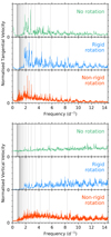Fig. 1.

Tangential (top panel) and vertical (bottom panel) velocity spectra predicted by the 2D IGW simulations from Rogers et al. (2013), for three scenarios for the radial rotation profile: no rotation; rigid rotation with a rotation frequency of 1.1 d⁻¹ (12.7 μHz); and non-rigid rotation (Ω_core/Ω_env = 1.5) with a surface rotational frequency of 0.275 d⁻¹ (8.7 μHz), which are shown in green, blue and red, respectively. We note that the amplitudes of these spectra have been normalised to the dominant peak in each spectrum and have arbitrary units. The vertical grey lines show the theoretical pulsation mode frequencies for (ℓ,m) = (1, 0) in a 3 M_⊙ ZAMS star for radial orders in the range n ∈ [−25, −1] calculated by GYRE (Townsend & Teitler 2013) and each rotation scenario.

3.2. IGW frequency comparison with `GYRE`

To further understand the IGW spectra from Rogers et al. (2013), we calculate a non-rotating 1D stellar structure model of a ZAMS 3 M_⊙ star using MESA (v9793; Paxton et al. 2011, 2013, 2015, 2018), and calculate its zonal dipole g-mode frequencies using the adiabatic module of GYRE (v5.0; Townsend & Teitler 2013; Townsend et al. 2018). The IGW frequency spectra shown in Fig. 1 have known rotation profiles from Rogers et al. (2013), hence we employ the traditional approximation for rotation (TAR) within GYRE when calculating numerical g-mode pulsation frequencies, with uniform rotation for the rigidly rotating model, and differential rotation as derived by Mathis (2009) and recently demonstrated by Van Reeth et al. (2018) for the non-rigid model. The frequencies corresponding to (ℓ,m) = (1, 0) for n ∈ [−25, −1] are overplotted on the IGW spectra as vertical grey lines in Fig. 1 for comparison. For a given radial order n, higher angular degrees ℓ have higher frequencies, which is why the IGW spectra in Fig. 1 appear structured, since these spectra contain many values of n, ℓ and m and thus contain hundreds of individual IGWs.

For all three scenarios of rotation in the tangential velocity spectrum in the top panel of Fig. 1, a series of dominant peaks are present between 1 ≲ ν ≲ 4 d⁻¹ (10 ≲ ν ≲ 50 μHz). Precise frequencies cannot be extracted from the IGW simulations using classical pre-whitening techniques because of the stochastic nature of the driving mechanism which produces broad peaks. However, if one assumes that the dominant peaks seen in Fig. 1 correspond to zonal dipole modes, (ℓ,m) = (1, 0), then one can see that they appear close to the pulsation mode frequencies calculated using GYRE, as such they are approximately equal to consecutive radial order modes in the range of n ∈ [−9, −5] with a characteristic period spacing between Δ P ≃ 4000−5000 s. This is consistent with the expected asymptotic period spacing for a ZAMS 3 M_⊙ star (Pápics et al. 2017; Pedersen et al. 2018). A similar interpretation is obtained if one makes a comparison to zonal quadrupole, retrograde dipole or prograde dipole g-mode frequencies using GYRE. Therefore, we speculate that the dominant peaks in the 2D IGW spectra from Rogers et al. (2013) correspond to g-mode pulsation frequencies that are stochastically excited through resonance, yet we cannot claim a unique identification of individual mode geometries for a given frequency. This interpretation is supported by the study of the Be star HD 51452, which was concluded to exhibit gravito-inertial modes that were stochastically excited by a convective region and produced broad peaks with variable amplitudes in the observed frequency spectrum (Neiner et al. 2012).

A detailed quantitative comparison of individual pulsation mode frequencies using GYRE and the theoretical IGW spectra from Rogers et al. (2013) must await 3D IGW numerical simulations. Yet, there are two important conclusions from the comparison of the 2D IGW spectra and GYRE, which are relevant for the characterisation of photometric variability due to an entire spectrum of IGWs, containing both travelling and standing wave components: (i) the dominant broad peaks in the IGW spectra are compatible with standing g-mode pulsation Eigenfrequencies, which we interpret to be stochastically-excited; and (ii) the background low-frequency power excess is caused by a spectrum of IGWs of various scales, which can be decomposed in multiple spherical harmonics of various ℓ and m values. It is the goal of this study to interpret the observational signatures of this background low-frequency power excess caused by a spectrum of IGWs in photometry. Specifically, we aim to measure the characteristic frequency and slope of the low-frequency power excess for stars across the HR diagram, as these observables provide useful constraints to the theory and numerical simulations of IGWs and angular momentum transport (Rogers et al. 2013; Rogers 2015).

4. Parameterising photometric red noise in massive stars

4.1. CoRoT stars of spectral types O, B, A and F

To perform a systematic search for IGWs across a wide range in stellar mass, we use the most recent, high-quality and high-cadence photometry from the CoRoT satellite (Auvergne et al. 2009). We use only a single telescope to avoid introducing biases from the differences in instrument passbands and sampling frequencies of other space missions. The early-type stars included in our study are stars of spectral type O, B, A and F from the CoRoT asteroseismology runs IRa01, LRa02, SRa01, SRa02, SRa03, SRa04, SRc01 and SRc02, with the specific details for each star, including the V-band magnitude, spectral type and fundamental parameters given in Table 1.

Table 1.

Properties of the stars included in this work.

We note that spectroscopic studies prior to the last decade typically have larger estimates of v sin i values for massive O and B stars as only rotational broadening was assumed and macroturbulence was usually ignored. Furthermore, estimates derived from only a single spectrum represent only a snapshot of the true variability, which explains why typically a variance of 20 km s⁻¹ is often found in literature values of v sin i and v_macro for O and B stars – see Table 1 of Aerts et al. (2014).

The CoRoT light curves range in length between ∼25 and ∼115 d and have a median cadence of approximately 32 s (Michel et al. 2006). The CoRoT satellite has an orbital frequency of 13.972 d⁻¹ (161.7 μHz) and its orbit crosses the South Atlantic Anomaly (SAA) twice each sidereal day, which introduces alias frequencies in a spectrum because of invalid flux measurements and periodically discarded hot pixels. The spectral window of CoRoT data is shown in Fig. 2, using the 34-d time series of HD 46150.

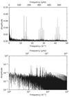Fig. 2.

Spectral window function of the CoRoT data for HD 46150 up to 50 d⁻¹ (578.7 μHz) on a linear scale (top panel) and on a logarithmic scale (bottom panel).

4.2. Pre-whitening of high signal-to-noise peaks

Amongst our sample are stars with coherent pulsation modes, including for example δ Sct, SPB and β Cep pulsators. The coherent pulsation modes in these stars can be p and g modes, which are driven by an opacity or heat engine driving mechanism and have periods of order hours and days (Aerts et al. 2010). The mode lifetimes of coherent pulsation modes are essentially infinite compared to the length of our observations, hence they can be extracted using iterative pre-whitening if time series data of sufficient length is available (see, e.g. Degroote et al. 2009; Pápics et al. 2012; Aerts et al. 2010; Bowman 2017).

Since we are interested in characterising the morphology of the background low-frequency power excess caused by a spectrum of IGWs, representing spherical harmonics of multiple ℓ and m values, we remove S/N > 4 peaks corresponding with the detected standing waves via pre-whitening (see e.g. Breger et al. 1993). The number of peaks extracted depends on the quality and quantity of photometric data available for an individual star. The noise level for each extracted peak is calculated using a window of 1 d⁻¹ centred at the extracted frequency, which in reality is an estimate that includes instrumental noise, white noise and any low-S/N astrophysical signal. Hence our conservative approach to pre-whitening by allowing for a local S/N estimate of a peak in a spectrum ensures we are not overfitting (Degroote et al. 2009; Pápics et al. 2012). Several studies have warned against the over-extraction of hundreds of frequencies using iterative pre-whitening, with this method injecting variability rather than removing it in the cases with variable amplitude and/or frequency peaks or strongly correlated data sets (see, e.g. Degroote et al. 2009; Pápics et al. 2012; Pascual-Granado et al. 2015; Kurtz et al. 2015; Bowman 2017). We opt for this conservative approach to only pre-whitening high-S/N peaks since we are interested in parameterising the background low-frequency power excess in a spectrum. This pre-whitening methodology produces a residual light curve, from which we calculate a residual power density spectrum in units of ppm²/μHz versus μHz to allow for an accurate comparison of stochastic signal in stars with different length CoRoT runs.

In the summary figures for these stars, we show the original and residual power density spectra in orange and black, respectively, in Appendix A. In stars for which pre-whitening was employed, the residual power density spectra represent our observations. The only exceptions were HD 46150 and HD 46223, in which no peaks with S/N ≥ 4 were detected. Thus we used the original power density spectra as our data for HD 46150 and HD 46233, and the residual power density spectra as our data for all other stars to search for signatures of IGWs.

4.3. Red noise fitting with a Bayesian MCMC numerical scheme

Following Stanishev et al. (2002) and Blomme et al. (2011), but also numerous studies of solar-like oscillators (see e.g. Michel et al. 2008; Chaplin & Miglio 2013; Kallinger et al. 2014; Hekker & Christensen-Dalsgaard 2017), the morphology of a stochastically-excited low-frequency power excess in a power density spectrum can be physically interpreted by a Lorentzian function:

$\begin{matrix} α (ν) = \frac{α_{0}}{1 + {(\frac{ν}{ν_{char}})}^{γ}} + P_{W}, \end{matrix}$ $\begin{aligned} \alpha \left( \nu \right) = \frac{ \alpha _{0} }{ 1 + \left( \frac{\nu }{\nu _{\rm char}} \right)^{\gamma }} + P_{\rm W} , \end{aligned}$ (1)

where α₀ is a scaling factor and represents the amplitude at zero frequency, γ is the gradient of the linear part of the profile in a log-log plot, ν_char is the characteristic frequency and P_W is a frequency-independent (i.e. white) noise term. The characteristic frequency (i.e. the frequency at which the amplitude of background equals half of α₀) is the inverse of the characteristic timescale: ν_char = (2πτ)⁻¹.

Previously, Blomme et al. (2011) discussed how the difference in the parameters of α₀, τ and γ may be related to the mass and evolutionary stage of the O stars HD 46150, HD 46223 and HD 46966. Specifically, HD 46966 is more evolved than HD 46223 and HD 46150, such that the fundamental parameters of HD 46966 may define the different morphology of the observed red noise. Furthermore, Blomme et al. (2011) also clearly demonstrate that this red noise is not instrumental, since different stars required different profiles. In this work, we extend the morphology characterisation of the photometric low-frequency power excess to more stars observed by CoRoT. We are motivated by the use of Eq. (1) as stochastic signals in the time domain are well-represented by Lorentzian profiles in the Fourier domain. Furthermore, the fitting parameters of ν_char and γ provide observables that can be directly compared to predictions from IGW simulations.

In our study, we use a Markov chain Monte Carlo (MCMC) numerical scheme within a Bayesian framework using the python emcee package (Foreman-Mackey et al. 2013), which is an ensemble, affine-invariant approach to sampling the parameter posterior distributions and provides a rigorous error assessment of the individual model parameters. Previous examples of this approach within asteroseismology include deriving orbital parameters for binary systems (Hambleton 2016; Schmid & Aerts 2016; Johnston et al. 2017; Hambleton et al. 2018; Kochukhov et al. 2018), peak-bagging of solar-like oscillations (e.g. Toutain & Appourchaux 1994; Appourchaux et al. 1998, 2008; Appourchaux 2003, 2008; Benomar et al. 2009; Gaulme et al. 2009; Gruberbauer et al. 2009; Handberg & Campante 2011; Davies et al. 2016), and extraction of unresolved pulsation mode frequencies in δ Sct stars (Bowman 2016, 2017). In our usage, the CoRoT residual power density spectra in the frequency range 1 ≤ ν ≤ 15 500 μHz are the data, the model and its parameters are given in Eq. (1). Since we are using the same model for all stars, we opt to use non-informative (flat) priors for all parameters and 128 parameter chains. At every iteration, each parameter chain is used to construct a model and is subject to a log-likelihood evaluation of:

$\begin{matrix} ln L \propto - \frac{1}{2} \sum_{i} {(\frac{y_{i} - M (Θ_{i})}{σ_{i}})}^{2}, \end{matrix}$ $\begin{aligned} \ln \mathcal{L} \propto - \frac{1}{2} \sum _i \left( \frac{\textit{y}_i - M(\Theta _i)}{\sigma _i} \right)^{2} , \end{aligned}$ (2)

where ln ℒ is the log-likelihood, y_i are the data, σ_i are their uncertainties and M_Θ is the model produced with parameters Θ. Since Eq. (2) uses an unnormalised χ² statistic, then ln ℒ converges to approximately −0.5n, where n is the number of data points. Typically, the first few hundred iterations are burned, but the exact number varies from star to star. Convergence is confirmed using the parameter variance criterion from Gelman & Rubin (1992), which is typically achieved after approximately 1000 iterations, and we produced the posteriors for the remaining ∼1000 iterations.

The results of our analysis for the O star HD 46150 are shown in Fig. 3, in which the top panel shows the logarithmic power density spectrum and the best-fit of Eq. (1) shown as a solid green line³. The middle panel of Fig. 3, shows the marginalised posteriors of each parameter as 1D histograms and 2D contours with the red and green crosses corresponding to the 68% and 95% credible levels, respectively. 1σ statistical uncertainties of each parameter are determined from a Gaussian fit to each histogram of the converged MCMC parameter chains. The numbers in the top-right sub-plots of the middle panel in Fig. 3 give the pair-wise correlation between parameters, with 1 indicating direct correlation and −1 indicating direct anti-correlation. The output parameters and their respective uncertainties for each star in our study are given in Table 2.

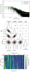Fig. 3.

Top panel: logarithmic power density spectrum of the CoRoT photometry for the O star HD 46150 is shown in black, and the best-fit model obtained using Eq. (1) is shown as the solid green line, with its red and white components shown as red short-dashed and blue long-dashed lines, respectively. Middle panel: posterior distributions from the Bayesian MCMC, with best-fit parameters obtained from Gaussian fits (shown in black) to the 1D histograms (shown in blue). Bottom panel: a sliding Fourier transform in the (linear) frequency range of 0 ≤ ν ≤ 4 d⁻¹ using a 15-d bin and a step of 0.1 d.

Table 2.

Optimised parameters for the extracted red noise (cf. Eq. (1)) for the stars studied in this paper using our Bayesian MCMC method, and the dominant cause(s) that are likely contributing to the observed low-frequency power excess, which are not only sourced from this work but also from the literature.

Similar summary figures for the O stars HD 46223 and HD 46966 are shown in Figs. 4 and 5, respectively, and all other summary figures are given in Appendix A. Most of our stars have undergone pre-whitening such that the original and residual spectra are shown as orange and black lines, respectively, expect for HD 46150 and HD 46233 in which the original spectra (shown in black) were used as the data as no significant (S/N ≥ 4) peaks were present in their spectra.

Fig. 4.

Summary figure for the O star HD 46223, which has a similar layout as shown in Fig. 3.

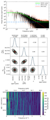Fig. 5.

Summary figure for the O star HD 46966, which has a similar layout as shown in Fig. 3, except that the original and residual power density spectra are shown in orange and black, respectively, since HD 49666 underwent pre-whitening of peaks with amplitude S/N ≥ 4.

4.4. Sliding Fourier transforms

Another commonly used method to demonstrate stochastic signal is the use of sliding Fourier transforms (SFTs), in which frequency spectra for moving subsets of a time series are calculated and stacked into a 2D image. The length of CoRoT data for some of the stars in our sample is ∼25 d, so the choice of the bin length and step size in an SFT is a compromise between temporal and frequency resolution. If the bin length is too short then a poor frequency resolution is obtained, but if it is too long, then the number of steps in an SFT will be too few to investigate any time-dependent behaviour. The SFTs for the O-stars HD 46150, HD 46223 and HD 46966 are shown in the bottom panels of Figs. 3–5, respectively, in which 15-d bins and a step size of 0.1 d are used for the frequency range between 0 ≤ ν ≤ 4 d⁻¹ (0 ≤ ν ≤ 46.3 μHz). Clearly, as previously noted by Blomme et al. (2011), the dominant low-frequency peaks in these three O stars are not coherent and have short lifetimes of order hours and days. Similar SFTs for all other stars are given in Appendix A.

5. Results: application to CoRoT stars

For each star given in Table 1, we applied our Bayesian MCMC methodology to determine the optimum values of α₀, ν_char, γ and P_W given in Eq. (1) and their respective uncertainties using the available CoRoT photometry. However, some of the stars in our sample are (known) pulsators with multiple high-S/N peaks in their frequency spectra representing coherent pulsation mode frequencies. Notable examples include the aforementioned δ Sct stars HD 50844 and HD 174936, with each of these stars claimed to have hundreds of independent coherent pulsation modes (Poretti et al. 2009; García Hernández et al. 2009). In this paper, we characterise the morphology of the background low-frequency power excess, so as previously discussed, coherent pulsation modes with S/N ≥ 4 were removed by iterative pre-whitening prior to employing the Bayesian MCMC methodology, as they affect the parameter estimation of the best-fitting red noise model of the residual power density spectra.

Our results are summarised in Table 2, in which we also indicate the causes of the variability observed for each star, with specific details given in the text. However, for some of the stars in our sample, the observational time base and resultant frequency resolution was insufficient to resolve and reliably extract all the pulsation modes via iterative pre-whitening. This resulted in some stars having localised “bumps” of unresolved pulsation modes or a flat noise plateau in their residual power density spectra, which impact the reliability of the background fit. We provide the MCMC fits for all stars for completeness, but have separated those stars significantly affected by the limitations of CoRoT data in Table 2.

5.1. HD 46150

HD 46150 is a young main-sequence O dwarf, which was first observed by Plaskett & Pearce (1931), and is the second hottest star in the cluster NGC 2244. It has an age of a few Myr (Bonatto & Bica 2009; Martins et al. 2012) and a spectral type of O5 V((f))z (Sota et al. 2011a,b). HD 46150 is suspected of being a long-period (P_orb ∼ 100 000 yr) binary system, because multiple nearby faint (Δ V ≥ 5 mag) stars having been detected in interferometry (Mason et al. 1998, 2001; Maíz Apellániz 2010; Sana et al. 2014; Aldoretta et al. 2015), and large radial velocity shifts in spectroscopy (e.g. Abt & Biggs 1972; Liu et al. 1989; Underhill & Gilroy 1990; Fullerton 1990; Fullerton et al. 2006; Mahy et al. 2009; Martins et al. 2012; Chini et al. 2012).

The known spectroscopic parameters of HD 46150 include an effective temperature of T_eff = 42 000 K and a surface gravity of log g = 4.0 (Martins et al. 2012, 2015), but its projected surface rotational velocity varies in the literature between 66 and 100 km s⁻¹ (Mahy et al. 2009; Martins et al. 2012, 2015; Simón-Díaz & Herrero 2014; Grunhut et al. 2017), with an average value of v sin i ≃ 80 km s⁻¹. Similarly, the macroturbulent velocities of HD 46150 also range between 37 and 176 km s⁻¹ (Martins et al. 2012, 2015; Simón-Díaz & Herrero 2014; Grunhut et al. 2017). HD 46150 was included as a target in the BOB campaign (Morel et al. 2014, 2015) and MiMeS survey (Wade et al. 2016), but null detections of a large-scale magnetic field were obtained by Fossati et al. (2015) and Grunhut et al. (2017).

As previously discussed by Blomme et al. (2011) and demonstrated in Fig. 3, HD 46150 clearly has a broad low-frequency power excess in its power density spectrum. Theoretical models were unable to explain the astrophysical red noise as coherent pulsation modes because of the inherent stochastic variability and Blomme et al. (2011) concluded that sub-surface convection, granulation, or inhomogeneities in the stellar wind were plausible explanations. Later, Aerts & Rogers (2015) interpreted the stochastic variability and red noise as IGWs. The summary figure showing the morphology of the red noise in the CoRoT photometry and the SFT for HD 46150 is given as Fig. 3.

5.2. HD 46223

HD 46223 is the hottest star in the cluster NGC 2244 with an age of a few Myr (Hensberge et al. 2000; Bonatto & Bica 2009; Martins et al. 2012), and a spectral type of O4 V((f)) (Underhill & Gilroy 1990; Massey et al. 1995; Sota et al. 2011a,b) or O4 V((f+)) (Maíz-Apellániz et al. 2004; Martins et al. 2005; Mokiem et al. 2007; Mahy et al. 2009). Although a faint companion star has been detected for HD 46223 (Mason et al. 2001; Turner et al. 2008), long-term spectroscopic campaigns have not revealed any significant radial velocity variations (e.g. Maíz-Apellániz et al. 2004; Fullerton et al. 2006; Mahy et al. 2009; Maíz Apellániz 2010; Chini et al. 2012; Schöller et al. 2017).

The known spectroscopic parameters of HD 46223 include an effective temperature of T_eff = 43 000 K and a surface gravity of log g = 4.0 (Martins et al. 2012, 2015). The projected surface rotational velocity of HD 46223 has a large variance in the literature with values that range from 58 to 100 km s⁻¹ (Mahy et al. 2009; Martins et al. 2012, 2015; Simón-Díaz & Herrero 2014; Grunhut et al. 2017), with an average value of approximately v sin i ≃ 80 km s⁻¹. Similarly, the macroturbulent velocities also range from 32 to 156 km s⁻¹ (Martins et al. 2012, 2015; Simón-Díaz & Herrero 2014; Grunhut et al. 2017). Estimates of the mass-loss rate for HD 46223 using Hα include log Ṁ ≃ −5.8 (Puls et al. 1996; Fullerton et al. 2006) and log Ṁ ≃ −6.2 (Martins et al. 2012). HD 46223 was included as a target in the BOB campaign (Morel et al. 2014, 2015) and MiMeS survey (Wade et al. 2016), but null detections of a large-scale magnetic field were obtained by Fossati et al. (2015) and Grunhut et al. (2017).

Similarly to HD 46150, HD 46223 also has a significant low-frequency power excess in its power density spectrum and stochastic variability in its SFT, which was interpreted as IGWs by Aerts & Rogers (2015). The summary figure showing the morphology of the red noise in the CoRoT photometry and the SFT for HD 46223 is given as Fig. 4.

5.3. HD 46966

HD 46966 is a slightly evolved O star in the Mon OB2 association (Mahy et al. 2009), and has a spectral type of O8.5 IV (Mahy et al. 2009; Sota et al. 2011a,b). Multiple faint objects (Δ V ≥ 5 mag) have been detected near to HD 46966 (Mason et al. 2001; Turner et al. 2008; Sana et al. 2014), although multi-epoch spectroscopy has yet to reveal strong evidence of binarity (see, e.g. Munari & Tomasella 1999; Maíz-Apellániz et al. 2004; Mahy et al. 2009; de Bruijne & Eilers 2012; Chini et al. 2012).

The known spectroscopic parameters of HD 46966 include an effective temperature of T_eff = 35 000 K and a surface gravity of log g = 3.9 (Martins et al. 2012, 2015). The projected surface rotational velocity of HD 46966 ranges from 33 to 50 km s⁻¹ in the literature (Mahy et al. 2009; Martins et al. 2012, 2015; Simón-Díaz & Herrero 2014; Grunhut et al. 2017), with an average value of v sin i ≃ 42 km s⁻¹. Similarly, the macroturbulent velocities of HD 46966 range from 27 to 90 km s⁻¹ (Martins et al. 2012, 2015; Simón-Díaz & Herrero 2014; Grunhut et al. 2017). HD 46966 was included as a target in the BOB campaign (Morel et al. 2014, 2015) and MiMeS survey (Wade et al. 2016), but null detections of a large-scale magnetic field were obtained by Fossati et al. (2015) and Grunhut et al. (2017).

Similarly to HD 46150 and HD 46223, HD 46966 has a significant low-frequency power excess interpreted as evidence for IGWs (Aerts & Rogers 2015), but there is also a dominant low-frequency peak in its spectrum which could be caused by rotational modulation. The summary figure showing the morphology of the red noise in the residual power density spectrum and the SFT after extracting this dominant peak for HD 46966 is given as Fig. 5.

5.4. HD 45418

HD 45418 (9 Mon) is a B5 V star, which is a member of the NGC 2232 cluster (Levato & Malaroda 1974; Baumgardt et al. 2000), and has an effective temperature of T_eff = 16 750 ± 130 K, a surface gravity of log g = 4.27 ± 0.04, and a projected surface rotational velocity of v sin i = 247 ± 8 km s⁻¹ (Lefever et al. 2010; Tetzlaff et al. 2011; McDonald et al. 2012; Bragança et al. 2012; Mugnes & Robert 2015). Previous investigations of the spectroscopic variability of HD 45418 have indicated that it may be a non-pulsating star (Adelman 2001; Lefever et al. 2010).

Our study is the first to analyse the CoRoT light curve of HD 45418, with its power density spectrum and SFT shown in Fig. A.1. Clearly, HD 45418 has multiple high-S/N low-frequency peaks in its power density spectrum, stochastic low-frequency variability, and a red noise background. Although it is not classified as a Be star, HD 45418 is a fast rotator and its pulsation modes between 0.3 ≤ ν ≤ 3 d⁻¹ (3 ≤ ν ≤ 30 μHz) may be stochastically-excited gravito-inertial modes, similar to those found in the Be star HD 51452 by Neiner et al. (2012). The summary figure showing the morphology of the red noise in the CoRoT photometry and the SFT for HD 45418 is given as Fig. A.1.

5.5. HD 45517

HD 45517 is a member of the cluster NGC 2232 (Claria 1972), and the only literature reference concerning its fundamental parameters is the determination is a spectral type as A0/2 V by Houk & Swift (1999). From analysis of its CoRoT photometry, we determine that HD 45517 has a low-frequency power excess and stochastic variability of order a few tens of μmag between 0 ≤ ν ≤ 20 d⁻¹ (0 ≤ ν ≤ 231 μHz). The summary figure showing the morphology of the red noise in the CoRoT photometry and the SFT for HD 45517 is given as Fig. A.2.

5.6. HD 45546

HD 45546 (10 Mon) is a member of the cluster NGC 2232 (Claria 1972), and has a spectral type of B2 V, an effective temperature of T_eff ≃ 19 000 K, a surface gravity of log g ≃ 4.0, and a projected surface rotational velocity of v sin i = 61 ± 3 km s⁻¹ (Lyubimkov et al. 2000, 2002, 2013; Abt et al. 2002; Tetzlaff et al. 2011; Bragança et al. 2012; Silaj & Landstreet 2014). HD 45546 has no strong evidence of being a binary or multiple system (Abt & Cardona 1984; Eggleton & Tokovinin 2008), but its spectroscopic variability revealed line profile variability that was indicative of high-ℓ pulsation modes (Telting et al. 2006). As the first study to investigate the photometric variability of HD 45546 using CoRoT observations, we confirm the presence of significant low-frequencies in its power density spectrum, as shown in Fig. A.3. Furthermore, we find that the low-frequency power excess in HD 45546 is stochastic, which could be caused by either unresolved coherent pulsation modes or damped pulsation modes. The summary figure showing the morphology of the red noise in the CoRoT photometry and the SFT for HD 45546 is given as Fig. A.3.

5.7. HD 46149

HD 46149 is a member of the young cluster NGC 2244 and was first observed by Plaskett & Pearce (1931). Later it was suspected of being a binary system because of variance in its radial velocity (Abt & Biggs 1972; Liu et al. 1989; Maíz-Apellániz et al. 2004; Turner et al. 2008). More recent studies have confirmed HD 46149 as an O8 V + B0/1 V long-period binary system with an orbital period of P_orb = 829 ± 4 d and an eccentricity of e = 0.59 ± 0.02 (Mahy et al. 2009; Degroote et al. 2010c; Sota et al. 2011a,b; Chini et al. 2012; Martins et al. 2012).

The known spectroscopic parameters of the O8 V primary include an effective temperature of T_eff = 36 000 K and a surface gravity of log g = 3.7, and an effective temperature of T_eff = 33 000 K and a surface gravity of log g = 4.0 for the B0/1 V secondary (Degroote et al. 2010c). The projected surface rotational velocity of the primary ranges between ∼0 and 78 km s⁻¹ in the literature (Degroote et al. 2010c; Martins et al. 2012, 2015; Simón-Díaz & Herrero 2014), with an average value of v sin i ≃ 30 km s⁻¹, and approximate value of v sin i ≃ 100 km s⁻¹ for the secondary (Martins et al. 2012). Similarly, macroturbulent velocities range from 24 to 61 km s⁻¹ for the primary (Martins et al. 2012, 2015; Simón-Díaz & Herrero 2014) and approximately 27 km s⁻¹ for the secondary (Martins et al. 2012). HD 46149 was included as a target in the BOB campaign (Morel et al. 2014, 2015) and MiMeS survey (Wade et al. 2016), but null detections of a large-scale magnetic field were obtained by Fossati et al. (2015) and Grunhut et al. (2017).

Previously, the 34-d CoRoT light curve of HD 46149 was analysed by Degroote et al. (2010c), who found evidence for pulsation modes between 3.0 < ν < 7.5 d⁻¹ (35 < ν < 87 μHz) that have have variable amplitudes, short lifetimes, and a characteristic frequency spacing of Δ ν = 0.48 ± 0.02 d⁻¹ (5.6 ± 0.2 μHz). These pulsation modes were postulated to be p modes excited by turbulent pressure in a sub-surface convection zone since coherent p modes excited by the opacity mechanism are not expected for such a star (Degroote et al. 2010c; Belkacem et al. 2010). However, as demonstrated in Fig. A.4, HD 46149 has an underlying stochastic low-frequency background in its residual power density spectrum, which is indicative of IGWs.

5.8. HD 46179

First classified by Merrill et al. (1925), HD 46179 is a known binary system with a B9 V primary (Dommanget & Nys 2000; Mason et al. 2001; Fabricius et al. 2002; Gontcharov 2006), an effective temperature of T_eff = 10 500 ± 500 K, a surface gravity of log g = 4.0 ± 0.2, and a projected surface rotational velocity of v sin i = 152 ± 13 km s⁻¹ (Niemczura et al. 2009; Degroote et al. 2011). Using ∼30 d of CoRoT photometry, Degroote et al. (2010b, 2011) found no significant periodicity indicative of coherent pulsation modes in HD 46179, which is not surprising since HD 46179 is located between the SPB and δ Sct instability regions and is not predicted to pulsate. In this work, we confirm the lack of coherent pulsation modes in HD 46179, but demonstrate that it has stochastic low-frequency variability between 0 ≤ ν ≤ 2 d⁻¹ (0 ≤ ν ≤ 23 μHz) in its power density spectrum, as shown in Fig. A.5. We also note, like Degroote et al. (2010b, 2011), that there is a dominant peak at an approximate frequency of ν ≃ 0.07 d⁻¹ (0.8 μHz) which could be caused by rotational modulation. HD 46179 is an interesting case study of an almost constant intermediate-mass star in our sample, thus its low-frequency power excess provides a useful upper constraint of the photometric amplitudes of order a few μmag for IGWs in a main sequence ∼3 M_⊙ late-B star.

5.9. HD 46202

HD 46202 is a young late-O dwarf and was first observed by Plaskett & Pearce (1931). It has a spectral type of O9.5 V (Walborn & Fitzpatrick 1990; Martins et al. 2005; Walborn et al. 2011; Sota et al. 2011a,b) or O9.2 V (Sota et al. 2014). Some studies inferred HD 46202 to have variable radial velocities (e.g. Abt & Biggs 1972), yet more recent dedicated spectroscopic campaigns show that HD 46202 is likely a single star (Underhill & Gilroy 1990; Mahy et al. 2009; Chini et al. 2012; Schöller et al. 2017). The spectroscopic parameters of HD 46202 include an effective temperature of T_eff = 33 000 K and a surface gravity of log g = 4.0 (Martins et al. 2005; Martins et al. 2012, 2015). The projected surface rotational velocity of HD 46202 ranges between 15 and 21 km s⁻¹ (Simón-Díaz & Herrero 2014; Martins et al. 2012, 2015) with an average value of v sin i ≃ 19 km s⁻¹. Similarly, the macroturbulent velocities of HD 46202 range between 13 and 58 km s⁻¹ (Simón-Díaz & Herrero 2014; Martins et al. 2012, 2015). HD 46202 was included as a target in the BOB campaign (Morel et al. 2014, 2015) and MiMeS survey (Wade et al. 2016), but null detections of a large-scale magnetic field were obtained by Fossati et al. (2015) and Grunhut et al. (2017).

Previously, Briquet et al. (2011) analysed the CoRoT photometry of HD 46202 and performed an asteroseismic analysis to identify p modes and perform forward seismic modelling. The authors determined a step convective core overshooting parameter of α_ov = 0.10 ± 0.05, but emphasise that none of the observed pulsation modes were predicted to be excited by theoretical models. More recently, Moravveji (2016) investigated the changes in the location of β Cep instability region after artificially enhancing the iron opacity by ∼75 percent. This alternative instability region includes HD 46202 and may provide an explanation for the observed pulsation mode frequencies.

HD 46202 is one of the more interesting stars in our study, with its summary figure shown in Fig. A.6. Its power density spectrum contains a few significant peaks, including ν ≃ 2.29, 2.64, and 3.00 d⁻¹ (26.5, 30.6 and 34.7 μHz, respectively), which Briquet et al. (2011) interpret as β Cep pulsations. These frequencies are similar to the dominant IGW frequencies shown in Fig. 1. After pre-whitening these significant peaks, HD 46202 also has an underlying background red noise profile and low-frequency stochastic variability in its residual power density spectrum, as shown in Fig. A.6, which is indicative of IGWs.

5.10. HD 46769

HD 46769 is a blue supergiant and a confirmed non-magnetic single star with a spectral type of B5 II, an effective temperature of T_eff = 13 000 ± 1000 K, a surface gravity of log g = 2.7 ± 0.1, and a projected surface rotational velocity of v sin i = 72 ± 2 km s⁻¹ (Houk & Swift 1999; Abt et al. 2002; Lefever et al. 2007; Zorec et al. 2009; Aerts et al. 2013; Wade et al. 2016). The CoRoT light curve and high-S/N, high-resolution spectroscopy of HD 46769 were previously analysed by Aerts et al. (2013), which revealed rotational modulation with multiple harmonics and a rotation period of 9.69 d. Their analysis also revealed a lack of coherent variability. The macroturbulence of HD 46769 was determined to be less than 10 km s⁻¹, which is much smaller than the measured rotational broadening and is atypically small for a blue supergiant (Aerts et al. 2013).

Similarly to other massive stars in our study, the lack of coherent periodicity in HD 46769 provides the opportunity to place constraints on the photometric low-frequency power excess in this blue supergiant (e.g. Aerts et al. 2018a). The morphology of the red noise in the CoRoT photometry after extracting the rotational modulation and the SFT for HD 46769 are shown in Fig. A.7. Our analysis of the blue supergiant HD 46769 revealed similar stochastic variability between 0 ≤ ν ≤ 3 d⁻¹ (0 ≤ ν ≤ 34.7 μHz) to that observed in the other blue supergiants HD 188209 (Aerts et al. 2017a) and HD 91316 (Aerts et al. 2018a), which suggests granulation from a surface convection zone or IGWs as plausible explanations.

5.11. HD 47485

HD 47485 has a spectral type of A5 IV/V (Houk & Swift 1999), an effective temperature of T_eff ≃ 7300 K, a surface gravity of log g ≃ 2.9, and a projected surface rotational velocity of v sin i ≃ 40 km s⁻¹ (Gebran et al. 2016). Our analysis of the CoRoT photometry of HD 47485 is the first analysis in the literature, and revealed intrinsic variability indicative of δ Sct pulsation modes between 6 ≤ ν ≤ 10 d⁻¹ (69 ≤ ν ≤ 116 μHz) as shown in its power density spectrum in Fig. A.8. However, the density of the peaks in this frequency range is extremely high and only ∼26 d of CoRoT photometry is not sufficient to resolve the beating and identify close-frequency pulsation modes (Bowman et al. 2016; Bowman 2017; Buysschaert et al. 2018). The residual pulsation signal in HD 47485 significantly affects the accuracy of our background fit. Therefore, we have labelled HD 47485 as having insufficient CoRoT data for an accurate background fit in Table 2. Nonetheless, we note the stochastic variability between 0 ≤ ν ≤ 3 d⁻¹ (0 ≤ ν ≤ 34.7 μHz) in HD 47485 which may be caused by granulation or IGWs.

5.12. HD 48784

HD 48784 has a literature spectral type of F0 V (Iijima & Ishida 1978) and an effective temperature of approximately T_eff ≃ 6900 K (McDonald et al. 2012). The CoRoT light curve of HD 48784 was previously studied by Barceló Forteza et al. (2017), who extracted 163 significant frequencies and detected a regular frequency spacing of Δ ν = 40.3 ± 0.6 μHz (≃3.5 d⁻¹). This was interpreted as the large frequency separation between consecutive radial order p modes, and from this an average density of $\bar{ρ} = 0.12 g {cm}^{- 3}$ $\bar{\rho} = 0.12 \,{\rm{g}}\,{\rm{c}}{{\rm{m}}^{ - 3}}$ and a mass of M = 2.0 ± 0.1 M_⊙ were derived for HD 48784 using scaling relations (Barceló Forteza et al. 2017). The low-frequency power excess in HD 48784 was interpreted to be related to the oblateness and rotation of the star, or the efficiency of the convective envelope (Barceló Forteza et al. 2017).

From the approximate mass of 2 M_⊙ and radius R = 2.8 R_⊙ from Barceló Forteza et al. (2017), one can easily calculate an approximate surface gravity of log g = 3.5, which we have included in Table 1. In our analysis of the CoRoT photometry of HD 48784, we extract 11 peaks that have S/N ≥ 4 between 0.5 ≤ ν ≤ 16.5 d⁻¹ (5.8 ≤ ν ≤ 191.0 μHz), which is far fewer than previous studies because our approach to iterative pre-whitening assumes non-white noise being present in the spectrum. The summary figure showing the morphology of the red noise in the CoRoT photometry and the SFT for HD 48784 is given as Fig. A.9.

5.13. HD 48977

HD 48977 (16 Mon) has a spectral type of B2.5 V, an effective temperature of T_eff ≃ 20 000 K, a surface gravity of log g ≃ 4.2, and a projected surface rotational velocity of v sin i ≃ 25 km s⁻¹ (Abt et al. 2002; Lyubimkov et al. 2005; Telting et al. 2006; Zorec et al. 2009; Hohle et al. 2010; Lefever et al. 2010; Thoul et al. 2013; Ahmed & Sigut 2017). In their previous analysis of the CoRoT photometry, Thoul et al. (2013) detect rotational modulation and infer a rotation frequency of ν = 0.6372 d⁻¹ (7.375 μHz), but also detect multiple g-mode pulsation frequencies. However, the ∼30-d length of the available CoRoT photometry limits the capability of identifying pulsation modes and subsequent modelling because of the poor frequency resolution, and since independent pulsation mode frequencies can be as close as 0.001 d⁻¹; 0.011 μHz (Bowman et al. 2016; Bowman 2017; Buysschaert et al. 2018).

In our analysis of the CoRoT photometry of HD 48977, we extract 12 peaks that have S/N ≥ 4 between 0.2 ≤ ν ≤ 1.3 d⁻¹ (2.3 ≤ ν ≤ 15.0 μHz), which are indicative of (unresolved) g-mode pulsation frequencies given that HD 48977 has a spectral type of B2.5 V. The low-frequency power excess in both the original and residual power density spectra of HD 48977 is clear, as demonstrated in the summary figure for HD 48977 in Fig. A.10, which supports the interpretation of damped pulsation modes in HD 48977 similar to those discussed by Aerts et al. (2017a, 2018a). However, we note that the complex CoRoT window pattern in HD 48977 results in a background fit which overestimates the white noise contribution. Thus we label HD 48977 as having insufficient data for an accurate background fit in Table 2, yet it is clear that this star still has a clear low-frequency power excess as shown in Fig. A.10.

5.14. HD 49677

HD 49677 is a slowly-rotating B9 V star, with an effective temperature of T_eff = 9200 ± 250 K and a surface gravity of log g = 4.0 ± 0.2, which were estimated using its spectral energy distribution (SED) by Degroote et al. (2011). If one assumes that the peak at ν ≃ 0.1 d⁻¹ (1.2 μHz) is the rotation frequency of HD 49677, a surface rotational velocity of order 10 km s⁻¹ can be derived, which is in agreement with the determination of HD 49677 as a slow rotator by Degroote et al. (2011). HD 49677 was also determined to be a candidate pulsator since it has frequencies between 0 ≤ ν ≤ 2 d⁻¹ (0 ≤ ν ≤ 23.1 μHz) in its spectrum (Degroote et al. 2011). However, HD 49677 lies outside of the δ Sct and SPB instability regions and is not expected to pulsate with coherent g modes. With no further analysis of HD 49677 having been performed since the study by Degroote et al. (2011), HD 49677 is another good example of stochastic low-frequency variability in a late-B star that cannot be explained as coherent pulsation modes, but can be explained by IGWs. The summary figure showing the morphology of the red noise in the CoRoT photometry and the SFT for HD 49677 is given as Fig. A.11.

5.15. HD 50747

HD 50747 has a spectral type of A4 IV, an effective temperature of T_eff ≃ 7500 K, a surface gravity of log g ≃ 3.5 and a projected surface rotational velocity of v sin i ≃ 70 km s⁻¹ (Royer et al. 2007; Zorec & Royer 2012; McDonald et al. 2012). However, Renson & Manfroid (2009) list a spectral type in the range of A4–A9 and flag HD 50747 as having possible chemical peculiarities. Dolez et al. (2009) previously analysed the CoRoT photometry of HD 50747 and found pulsation mode frequencies that they interpreted to be g modes. This star is also known to be a triple system from analysis of high-resolution spectroscopy as its spectra contain two narrow-line component stars and an additional broad-line component star (Eggleton & Tokovinin 2008; Dolez et al. 2009). Thus, Dolez et al. (2009) concluded that HD 50747 is a triple system containing a γ Dor star because of the spectroscopic parameters and observed range of pulsation mode frequencies.

From our analysis of the CoRoT light curve of HD 50747, we confirm the presence of significant low-frequency peaks in its power density spectrum, many of which are variable in amplitude and frequency as demonstrated in the SFT in the bottom panel of Fig. A.12. If the low-frequency power excess observed in HD 50747 is caused by coherent pulsation modes, then they are clearly not resolved with only ∼60 d of CoRoT observations, which would explain their apparent stochastic nature. On the other hand, IGWs can also explain the low-frequency power excess in HD 50747, although we cannot rule out granulation for HD 50747 since it is cool and evolved enough to have a surface convection zone. The summary figure showing the morphology of the red noise in the CoRoT photometry and the SFT for HD 50747 is given as Fig. A.12.

5.16. HD 50844

HD 50844 has a spectral type of A2 II (Houk & Swift 1999) and is one of the well-known δ Sct stars previously studied using CoRoT photometry (Poretti et al. 2005, 2009). From high-resolution spectroscopy, Poretti et al. (2009) derive an effective temperature of T_eff = 7400 ± 200 K, a surface gravity of log g = 3.6 ± 0.2 and a projected surface rotational velocity of v sin i = 58 ± 2 km s⁻¹. The frequency spectrum of HD 50844 is claimed to be dense enough to contain thousands of peaks, some of which were interpreted as prograde high-ℓ p modes from spectroscopic line profile observations (Poretti et al. 2009). Later the extremely high number of peaks extracted by Poretti et al. (2009) were interpreted by Kallinger & Matthews (2010) as part of a red noise background caused by granulation.

If the mode density in an frequency spectrum is sufficiently high such that peaks are not well-resolved from each other and/or the intrinsic pulsation modes exhibit amplitude or frequency modulation, the extraction of non-periodic variability using a pure (co)sinusoid leads to a vast over-estimate in the number of significant frequencies. This is because many fictitious and spurious frequencies will be injected into the light curve as part of the iterative pre-whitening process – see Balona (2014) for a detailed discussion of this problem using HD 50844 as a case study. Therefore, in cases where mode density is high it is more prudent to be conservative in the extraction of significant peaks and always check that individual frequencies are resolved from each other and that they are statistically significant beyond a simplistic S/N ≥ 4 criterion which assumes only white noise in a spectrum.

In our analysis of the CoRoT light curve of HD 50844, we extract 54 significant frequencies using our conservative approach to iterative pre-whitening. The summary figure showing the morphology of the red noise in the CoRoT photometry extracted using our Bayesian MCMC fit and the SFT for HD 50844 is given as Fig. A.13. We emphasise that the remaining variance in the residual power density spectrum, shown in black in Fig. A.13 has an amplitude S/N < 4. As discussed by Poretti et al. (2009), the high mode density in HD 50844 produces an almost flat noise plateau below ν ≲ 30 d⁻¹ (ν ≲ 347 μHz) after the dominant peaks have been extracted, as shown in the top panel of Fig. A.13. The background signal in the residual power density spectrum, interpreted as granulation signal by Kallinger & Matthews (2010), may explain the steep red noise morphology obtained from our Bayesian MCMC red noise fit. Since the flat noise plateau in HD 50870 extends to approximately 100 μHz, it impacts the determination of the parameter γ when fitting any red noise background caused by IGWs that may be in this star. Thus we label HD 50844 in Table 2 as having insufficient CoRoT data to remove all pulsation modes, which subsequently affects the accurate determination of the fitting parameter γ.

5.17. HD 50870

HD 50870 has spectral types in the literature that range between F0 IV and A8 V (McCuskey 1956; Houk & Swift 1999; Mantegazza et al. 2012). High-resolution and high-S/N spectroscopy of HD 50870 revealed it to be long-period SB2 system with primary star having a spectral type of A8 III, an effective temperature of 7660 ± 250 K, a surface gravity of log g = 3.68 ± 0.25 and a projected surface rotational velocity of v sin i = 37.5 ± 2.5 km s⁻¹ (Mantegazza et al. 2012). The secondary star has a spectral type of F2 III, an effective temperature of 7077 ± 250 K, surface gravity of log g = 3.74 ± 0.25 and a projected surface rotational velocity of v sin i = 8.0 ± 2.5 km s⁻¹ (Mantegazza et al. 2012). With both stars having similar fundamental parameters, they are also in a very similar location within the classical instability strip so it cannot be uniquely claimed that the primary or secondary, or both stars are pulsating.

Over 1000 frequencies were extracted from the CoRoT light curve of HD 50870 by Mantegazza et al. (2012) and independently by Barceló Forteza et al. (2017). These studies found a regular frequency spacing of approximately 55 μHz (4.8 d⁻¹), which was interpreted as the large frequency separation and used to derive an average density of $\bar{ρ} = 0.17 g {cm}^{- 3}$ $\bar{\rho} = 0.17\,{\rm{g}}\,{\rm{c}}{{\rm{m}}^{ - 3}}$ and a mass of M = 1.5 M_⊙ (Suárez et al. 2014; Barceló Forteza et al. 2017). The numerous frequencies and the presence of a low frequency power excess in HD 50870 was interpreted to be either caused by granulation (Mantegazza et al. 2012), or related to the oblateness and rotation of the star (Barceló Forteza et al. 2017). It should be noted that Mantegazza et al. (2012) binned the high-cadence CoRoT light curve into 20535 data points with an effective Nyquist frequency of 100 d⁻¹ (1157 μHz) as part of their analysis. Consequently, such a significantly lower Nyquist frequency dramatically increases the amplitude suppression within a “long” cadence data set and suppresses astrophysical signal (see Sect. 2.3.3 of Bowman 2017).

Similarly to HD 50844, the high mode density of HD 50870 produces an almost flat noise plateau in the residual power density spectrum, which is shown in Fig. A.14. Since the flat noise plateau in HD 50870 extends to high frequencies, this impacts the determination of the fitting parameter γ, and limits the interpretation of any low-frequency power excess being caused by IGWs. Thus we label HD 50870 as having insufficient CoRoT data for an accurate determination of the fitting parameter γ in Table 2.

5.18. HD 51193

HD 51193 (V746 Mon) has a spectral type of B1.5 IVe, an effective temperature of T_eff ≃ 23 000 K, a surface gravity of log g ≃ 3.6 and a projected surface rotational velocity of 220 ± 25 km s⁻¹ (Frémat et al. 2006; Gutiérrez-Soto et al. 2011). From photometric and spectroscopic data sets, HD 51193 is known to be a multi-periodic pulsating star with its low-frequency variability previously interpreted as non-radial g modes (Gutiérrez-Soto et al. 2007, 2011; Lefèvre et al. 2009). The low-frequency power excess in the power density spectrum of HD 51193 is clear in addition to strong beating of unresolved frequencies, as demonstrated in Fig. A.15. Similarly to HD 45418, HD 51193 is a rapid rotator and not known to be a Be star, but the high-S/N peaks in the frequency range 1 ≤ ν ≤ 2 d⁻¹ (11.6 ≤ ν ≤ 23.1 μHz) may be stochastically-excited gravito-inertial modes like those found in the Be star HD 51452 by Neiner et al. (2012). The summary figure showing the morphology of the red noise in the CoRoT photometry and the SFT for HD 51193 is given as Fig. A.15. We note that the complex CoRoT window pattern in HD 51193 results in a background fit which overestimates the white noise contribution. Thus we label HD 51193 as having insufficient CoRoT data for an accurate background fit in Table 2, yet it is clear that this star still has a clear low-frequency power excess.

5.19. HD 51332

HD 51332 has a spectral type of F0 V (Houk & Swift 1999), an effective temperature of T_eff ≃ 6700 K and a surface gravity of log g ≃ 4.0 (Masana et al. 2006; Holmberg et al. 2009; Casagrande et al. 2011; Bailer-Jones 2011; McDonald et al. 2012; David & Hillenbrand 2015). The summary figure showing the morphology of the red noise in the CoRoT photometry after the significant peaks in the power density spectrum have been extracted and the SFT for HD 51332 is given as Fig. A.16. We also note that HD 51332 has a series of low-frequency harmonics in its power density spectrum, which suggests that it may be a binary system. The binarity of HD 51332 has also been inferred from radial velocity measurements (Frankowski et al. 2007).

5.20. HD 51359

HD 51359 has a spectral type of A9/F0 IV (Houk & Swift 1999) and an approximate effective temperature of T_eff ≃ 6800 K (McDonald et al. 2012). It is also a known visual double star determined using speckle interferometry at the US Naval Observatory, with a companion star that is Δ V ≃ 2 mag fainter (Germain et al. 1999; Douglass et al. 1999). HD 51359 is a δ Sct star with numerous p-mode frequencies, which similarly to HD 50844 and HD 50870, produce an almost flat noise plateau in the residual power density spectrum, as shown in Fig. A.17. This low-frequency power excess could be evidence of granulation since HD 51359 is a late-A/early-F star with a thin surface convection zone, or low-S/N p modes. The summary figure showing the morphology of the red noise in the CoRoT photometry and the SFT for HD 51359 is given as Fig. A.17. Since the flat noise plateau in HD 51359 impacts the determination of the fitting parameter γ, we label HD 51359 as having insufficient CoRoT data in Table 2.

5.21. HD 51452

HD 51452 is a rapidly-rotating Be star with a spectral type of B0 IVe, an effective temperature of T_eff = 29 000 ± 500 K, a surface gravity of log g = 3.95 ± 0.04, and a projected surface rotational velocity of v sin i = 315.5 ± 9.5 km s⁻¹ (Frémat et al. 2006; Neiner et al. 2012). From a combined analysis of CoRoT photometry and high-resolution, high-S/N spectroscopy, Neiner et al. (2012) discovered that HD 51452 exhibits stochastically-excited gravito-inertial pulsation modes that can be explained by the rapid rotation of this star. The stochastic excitation of gravito-inertial waves was predicted by Rogers et al. (2013) and Mathis et al. (2014). Inspired by these findings, it was suggested that the outburst phenomena seen in Be stars may be explained by angular momentum transport by IGWs in rapidly-rotating B stars (Neiner et al. 2013; Lee et al. 2014). The summary figure showing the morphology of the red noise in the CoRoT photometry and the SFT for HD 51452 is given as Fig. A.18. However, we note that the complex CoRoT window pattern in HD 51452 results in a background fit which overestimates the white noise contribution. Thus we label HD 51452 as having insufficient CoRoT data for an accurate background fit in Table 2, yet it is clear that this star still has a clear low-frequency power excess caused by pulsations.

5.22. HD 51722

HD 51722 has a spectral type of A9 V (Houk & Swift 1999) and an approximate effective temperature of T_eff ≃ 7000 K (McDonald et al. 2012). It is also known to a be a double star in the Tycho double star catalogue (Fabricius et al. 2002; Roberts et al. 2015), and has possible transit signatures in its CoRoT light curve (Liu et al. 2015). A possible detection of variability in HIPPARCOS photometry was made by Koen & Eyer (2002), but no studies since have used the available CoRoT light curve to investigate if HD 51722 exhibits coherent and/or damped pulsation modes. In our analysis of the CoRoT light curve of HD 51722, we extract almost 100 significant frequencies between 0 ≤ ν ≤ 20 d⁻¹ (0 ≤ ν ≤ 231 μHz) using our conservative approach to iterative pre-whitening, which makes this star similar to the other high-mode density δ Sct stars including HD 50844, HD 50870 and HD 51359, since it has an almost flat noise plateau in its residual power density spectrum. This background signal explains the steep red noise morphology obtained from our Bayesian MCMC fit and could be caused by granulation and/or low-S/N pulsation modes. The summary figure showing the morphology of the red noise in the CoRoT photometry and the SFT for HD 51722 is given as Fig. A.19. The flat noise plateau in HD 51722 extends to high frequencies, which affects the determination of the fitting parameter γ. Thus we label HD 51722 as having insufficient CoRoT data for an accurate determination of the fitting parameter γ in Table 2.

5.23. HD 51756

HD 51756 has a spectral type of B0.5 IV (Pápics et al. 2011) and is a visual double star in the Tycho double star catalogue (Fabricius et al. 2002). Pápics et al. (2011) previously studied the CoRoT photometry, combined it with high-resolution, high-S/N spectroscopy and discovered HD 51756 to be a long-period SB2 system. The primary is slow rotator (v sin i = 28 ± 4 km s⁻¹) and the secondary is a fast rotator (v sin i ≃ 170 ± 15 km s⁻¹), but both components have the same spectral type, similar effective temperatures of T_eff = 30 000 ± 1000 K and surface gravities of log g = 3.75 ± 0.25. Coherent heat-driven pulsation modes are expected for these stars but none were detected by Pápics et al. (2011). The CoRoT photometry of HD 51756 does contain signatures of rotational modulation which Pápics et al. (2011) speculated to be caused by surface abundance inhomogeneities. In our study using the latest CoRoT light curve of HD 51756, we confirm the absence of coherent pulsation modes. However, we note the presence of a significant low-frequency power excess which is indicative of IGWs, because both components of HD 51756 have a spectral type of B0.5 IV and are thus too hot to have granulation from a surface convection envelope. The summary figure showing the morphology of the red noise in the CoRoT photometry and the SFT for HD 51756 is given as Fig. A.20.

5.24. HD 52130

The only literature reference of HD 52130 is the determination of its spectral type as A2 III/IV by Houk & Swift (1999). Unfortunately, fundamental parameters of HD 52130 are not available, but from its spectral type we can estimate an effective temperature of T_eff = 8200 K. The summary figure showing the morphology of the red noise in the CoRoT photometry and the SFT for HD 52130 is given as Fig. A.21, which clearly shows stochastic low-frequency variability consistent with either granulation or IGWs.

5.25. HD 174532

HD 174532 (7 Aql) has a spectral type of A9 IV listed by Houk & Swift (1999), although later studies revealed it to be an evolved star with a spectral type of A2 III/IV, an effective temperature of approximately T_eff ≃ 7200 K, a surface gravity of log g ≃ 3.6 and a projected surface rotational velocity of v sin i ≃ 32 km s⁻¹ (Poretti et al. 2003; Fox Machado et al. 2008; Fox Machado et al. 2010; McDonald et al. 2012). HD 174532 was previously known to be a multi-periodic δ Sct star (Fox Machado et al. 2008, 2010), and in our analysis of the CoRoT photometry of HD 174532, we extract 33 frequency peaks with a S/N ≥ 4 using our conservative approach to iterative pre-whitening. As shown in Fig. A.22, HD 174532 has a bump excess of unresolved pulsation modes at ∼200 μHz in its residual power density spectrum. This is because only 26.24 d of CoRoT data are available making the removal of close-frequency (hence unresolved) pulsation modes practically impossible. Since this unresolved remaining signal impacts the determination of the fitting parameter γ, we label HD 174532 as having insufficient CoRoT data for an accurate fit in Table 2.

5.26. HD 174589

HD 174589 (8 Aql) has a spectral type of F0 IV listed by Houk & Swift (1999), although later studies revealed it to be an evolved star with a spectral type of F2 III, an effective temperature of approximately T_eff ≃ 7000 K, a surface gravity of approximately log g ≃ 3.5 and a projected surface rotational velocity of v sin i ≃ 97 km s⁻¹ (Poretti et al. 2003; Fox Machado et al. 2008, 2010; McDonald et al. 2012). Similarly to HD 174532, HD 174589 is also a known multi-periodic δ Sct star (Fox Machado et al. 2008, 2010). In our analysis of the CoRoT photometry, we extract 17 frequency peaks with a S/N ≥ 4 using our conservative approach to iterative pre-whitening, which reveals a low-frequency power excess in the residual power density spectrum that is indicative of granulation or IGWs. The summary figure showing the morphology of the red noise in the CoRoT photometry and the SFT for HD 174589 is given as Fig. A.23.

5.27. HD 174936

HD 174936 has a spectral type of A3 IV (Houk & Swift 1999), and Strömgren photometry indicates an effective temperature of T_eff = 8000 ± 200 K and surface gravity of log g = 4.1 ± 0.2 (Hauck & Mermilliod 1998). Later, García Hernández et al. (2009) obtained high-resolution spectroscopy, confirmed its fundamental parameters and measured a projected surface rotational velocity of v sin i ≃ 170 km s⁻¹. The CoRoT light curve of HD 174936 was previously analysed by García Hernández et al. (2009), who extracted 422 frequencies and found a regular frequency spacing of approximately 52 μHz (≃4.5 d⁻¹). This regular spacing was interpreted as the large frequency separation and used it to derive an average density of $\bar{ρ} = 0.33 g {cm}^{- 3}$ $\bar{\rho} = 0.33 \,{\rm{g}}\,{\rm{c}}{{\rm{m}}^{ - 3}}$ and a mass of M = 1.6 M_⊙ (García Hernández et al. 2009; Suárez et al. 2014).

In our analysis of the CoRoT photometry of HD 174936, we extract 64 frequency peaks with a S/N ≥ 4 using our conservative approach to iterative pre-whitening, which reveals an almost flat noise plateau in the residual power density spectrum up to 50 d⁻¹ (579 μHz) that could be caused by granulation and/or low-S/N pulsations. The summary figure showing the morphology of the red noise in the CoRoT photometry and the SFT for HD 174936 is given as Fig. A.24. The flat noise plateau likely caused by a high density of unresolved pulsation modes in HD 174936 and the insufficient frequency resolution to remove them via pre-whitening impacts the determination of the fitting parameter γ. Thus we label HD 174936 as having insufficient CoRoT data for an accurate determination of the fitting parameter γ in Table 2.

5.28. HD 174966

HD 174966 has a spectral type of A7 III/IV (Houk & Swift 1999), an effective temperature of T_eff = 7555 ± 50 K, a surface gravity of log g = 4.2 ± 0.1, and a projected surface rotational velocity of v sin i ≃ 126 km s⁻¹ determined from high-resolution, high-S/N spectroscopy (García Hernández et al. 2013). The CoRoT light curve of HD 174966 was previously analysed by García Hernández et al. (2013), who extracted 185 frequencies and detected a regular frequency spacing of approximately 65 μHz (≃5.6 d⁻¹), which was interpreted as the large frequency separation and used to derive an average density of $\bar{ρ} = 0.51 g {cm}^{- 3}$ $\bar{\rho} = 0.51 \, {\rm{g}}\,{\rm{c}}{{\rm{m}}^{ - 3}}$ and a mass of M = 1.7 ± 0.2 M_⊙. The combination of spectroscopy and Strömgren photometry also allowed García Hernández et al. (2013) to identify 18 frequencies between 18 ≤ ν ≤ 33 d⁻¹ (208.3 ≤ ν ≤ 381.9 μHz) as low-degree non-radial p modes.

In our analysis of the CoRoT photometry of HD 174966, we extract 42 significant frequencies with S/N ≥ 4 between 0 ≤ ν ≤ 51 d⁻¹ (590 μHz) using our conservative approach to iterative pre-whitening, which reveals a low-frequency power excess in the residual power density spectrum that could be caused by granulation and/or low-S/N pulsations. The summary figure showing the morphology of the red noise in the CoRoT photometry and the SFT for HD 174966 is given as Fig. A.25.

5.29. HD 174967

The only literature reference to HD 174967 is a spectral type of B9.5 V by Houk & Swift (1999), which we use to estimate an approximate effective temperature of T_eff ≃ 11 000 K. In our analysis of the CoRoT photometry for HD 174967, we note the absence of coherent pulsation modes in the power density spectrum, which is in agreement with the expectation from theory for a lack of pulsation in stars between the SPB and δ Sct instability regions. However, as shown in the summary figure of HD 174967 in Fig. A.26, there is a low-frequency power excess below ν ≲ 2 d⁻¹ (23 μHz) in the power density spectrum. The morphology of the red noise in the CoRoT photometry and the SFT for HD 174967 are shown in Fig. A.26.

5.30. HD 174990

The only literature reference to HD 174990 is a spectral type of A3 V by Houk & Swift (1999), which we use to estimate an approximate effective temperature of T_eff ≃ 8500 K. Similarly to HD 174967, the early-A star HD 174990 also lacks coherent pulsation modes but does have a clear low-frequency power excess below ν ≲ 2 d⁻¹ (23 μHz) in its power density spectrum. Since neither coherent gravity mode pulsations or granulation from a surface convection zone are not expected in early-A main-sequence stars, we interpret this stochastic variability as IGWs. The summary figure showing the morphology of the red noise in the CoRoT photometry and the SFT for HD 174990 is given as Fig. A.27.

5.31. HD 175272

The spectral type of HD 175272 is listed as A0 V and flagged as being a member of a multiple system by Houk & Swift (1999). Using medium-resolution spectroscopy, Prugniel & Soubiran (2001) determined a spectral type of F5 V and estimated an effective temperature of 6500 K and a surface gravity of log g = 4.1 for HD 175272. Later, Poretti et al. (2003) measured a projected surface rotational velocity of v sin i ≃ 23 km s⁻¹ and noted a lack of periodic photometric variability. In their catalogue of stellar parameters for stars observed by HIPPARCOS, McDonald et al. (2012) list an effective temperature of 6900 K for HD 175272. More recently, HD 175272 has been claimed to show solar-like pulsations by Ozel et al. (2013) and Hekker & Ball (2014), who derived an effective temperature of T_eff ≃ 6700 K, a mass of M ≃ 1.5 M_⊙, and a frequency of maximum amplitude ν_max ≃ 1500 μHz (≃130 d⁻¹). However, these parameters were determined by comparing the low-S/N detection of solar-like oscillations in HD 175272 to the seismically-similar star HD 181420.

HD 175272 is amongst the coolest stars in our sample with an effective temperature of T_eff ≃ 6700 K, which is certainly cool enough for it to have a surface convection zone. However, it is still massive enough to host a convective core that could excite IGWs. It is possible for stars of this temperature to exhibit coherent g-mode pulsation frequencies (i.e. γ Dor stars) but we do not detect any significant periodic variability in the CoRoT observations of HD 175272. We do find a significant low-frequency power excess, which is presumably dominated by granulation. The summary figure showing the morphology of the red noise in the CoRoT photometry and the SFT for HD 175272 is given as Fig. A.28.

5.32. HD 175445

HD 175445 is listed as an A1 V star by Houk & Swift (1999). Later, Paunzen et al. (2001, 2002) classified HD 175445 as a λ Boo star with a spectral type of hA5mA2V, an effective temperature of T_eff = 8520 ± 200 K and a surface gravity of log g = 3.96 ± 0.10. Although, the effective temperature may be as high as T_eff = 9060 ± 330 K (Murphy & Paunzen 2017). In our analysis of the CoRoT photometry, we extract 32 frequency peaks with a S/N ≥ 4 using our conservative approach to iterative pre-whitening, which reveals an almost flat noise plateau below ν ≲ 30 d⁻¹ (347 μHz) in the residual power density spectrum, which is indicative of granulation, low-S/N pulsation modes or IGWs. The summary figure showing the morphology of the red noise in the CoRoT photometry and the SFT for HD 175445 is given as Fig. A.29. Motivated by having only 26.24 d of CoRoT photometry, we label HD 175445 as having insufficient data for an accurate determination of the fitting parameter γ in Table 2, because its residual power density spectrum likely contains unresolved close-frequency pulsation modes.

5.33. HD 175542

The only literature reference of HD 175542 is the determination of its spectral type as A1 V by Houk & Swift (1999), but from its spectral type we can estimate an effective temperature of T_eff ≃ 8500 K. In our analysis of the CoRoT photometry of HD 175542, we find a lack of coherent pulsation modes but do find a clear low-frequency power excess below ν ≲ 2 d⁻¹ (23 μHz) in the power density spectrum. The morphology and stochastic nature of this low-frequency signal is similar to other early-A stars in our sample, which are not expected to have coherent g modes or granulation from a surface convection zone. The summary figure showing the morphology of the red noise in the CoRoT photometry and the SFT for HD 175542 is given as Fig. A.30, which clearly show evidence of low-frequency stochastic variability that we interpret as being caused by IGWs.

5.34. HD 175640

HD 175640 is a known non-magnetic chemically peculiar star with a spectral type of B9 V HgMn, an effective temperature of T_eff = 12 000 ± 100 K, a surface gravity of log g = 3.95 ± 0.15 and a projected surface rotational velocity of order a few km s⁻¹ (Hubrig et al. 2001; Dolk et al. 2002; Castelli & Hubrig 2004, Renson & Manfroid 2009; Landstreet et al. 2009; Lefever et al. 2010; Makaganiuk et al. 2011). In their previous analysis of the CoRoT light curve of HD 175640, Ghazaryan et al. (2013) concluded that there were no significant coherent pulsation modes. In our analysis, having excluded known CoRoT alias frequencies (e.g. see Fig. 2), we confirm that lack of significant coherent pulsation modes, but do detect a low-frequency power excess in the power density spectrum. The summary figure showing the morphology of the red noise in the CoRoT photometry and the SFT for HD 175640 is given Fig. A.31, which clearly show evidence of low-frequency stochastic variability.

5.35. HD 263425

The only literature reference of HD 263425 is the determination of its spectral type as A0 V by Voroshilov et al. (1985), which we use to estimate an effective temperature of approximately T_eff ≃ 9500 K. Similar to other early-A stars, which do not have coherent pulsation modes nor expected to have granulation from a surface convection zone, we detect a low-frequency power excess in the power density spectrum of HD 263425. The summary figure showing the morphology of the red noise in the CoRoT photometry and the SFT for HD 263425 is given as Fig. A.32, which clearly show evidence of low-frequency stochastic variability that we interpret as IGWs.

6. Discussion

Within our sample of O, B, A and F stars are pulsating stars that underwent pre-whitening to remove high-S/N peaks since the physical driving mechanism of these dominant frequencies cannot be determined from observations alone. For stars without significant limitations imposed by the length and quality of CoRoT photometry, the morphology of the background low-frequency power excess in stars after pre-whitening standing waves allows inference of the physics that is responsible for the stochastic low-frequency variability in photometric observations of early-type stars.

In addition to the three O stars studied by Blomme et al. (2011) and Aerts & Rogers (2015), there are two other O stars in our sample: HD 46149 and HD 46202. The CoRoT photometry of these stars have been previously analysed by Degroote et al. (2010c) and Briquet et al. (2011), respectively, with both stars showing evidence for intrinsic variability attributed to pulsation modes. However, these stars also have low-frequency stochastic variability in their power density spectra and a significant low-frequency power excess. Individual amplitudes of peaks in the background low-frequency power excess are of order tens and hundreds of μmag for these five O stars. Further down the main sequence are early-B stars, such as HD 45546, which also have similar characteristic frequencies, ν_char, and amplitudes, α₀, in the morphology of their red noise compared to the O stars. The similar morphology in the power density spectra of these O and B stars, is evidence for a common physical mechanism acting in these stars.

Amongst the A and F stars in our sample are several δ Sct stars, which contain dozens of high-frequency coherent standing pulsation modes that we removed via pre-whitening. However, these intermediate-mass stars also have a background low-frequency power excess of order 10 μmag (i.e. α₀≃ a few hundred ppm²/μHz in their residual power density spectra). For late-A and F stars it is plausible that the observed stochastic low-frequency variability is caused by granulation, but this cannot be true for O and B stars as these do not have surface convection zones whilst on the main sequence. We explore why the observed low-frequency power excess for many of the stars in our sample is not consistent with granulation in Sect. 6.2.

On the other hand, we clearly have early-A stars in our sample that are not expected to pulsate in coherent g-modes, such as HD 45517 and HD 263425, which have a significant low-frequency power excess in their power density spectra. It has been investigated using observations of variable stars in clusters and later followed up with theoretical work, that the rapid rotation of some SPB stars is sufficient to distort a star such that its measured parameters place it between the SPB and δ Sct instability regions in the HR diagram (Mowlavi et al. 2013; Salmon et al. 2014). However, the stars in our sample that fall within this region are slow or moderate rotators.

6.1. Asteroseismic HR diagrams

Following the methodology employed by Simón-Díaz et al. (2017) and Godart et al. (2017), who studied the distribution of macroturbulence in the spectroscopic HR diagram of massive stars, we use a spectroscopic proxy for stellar luminosity defined as $L = T_{eff}^{4} / g$ ${\cal L} = T_{{\rm{eff}}}^4/g$ . Using the available spectroscopic parameters for the 18 stars in our sample with sufficient CoRoT data for an accurate background fit of the residual power density spectrum, we place them in (spectroscopic) HR diagrams in the bottom row of Fig. 6, in which the filled circles in the left and right panels have been colour-coded by the red noise fit parameters ν_char and γ, respectively, and the symbol size is proportional to the red-noise parameter α₀. For completeness, we also include the location of stars with available spectroscopic parameters but insufficient CoRoT photometry for an accurate background fit of the residual power density spectrum as white triangles in Fig. 6. For illustrative purposes, the (non-rotating) evolutionary tracks for representative masses between 2 and 60 M_⊙ from Ekström et al. (2012) are shown as solid grey lines, with the ZAMS line indicated by the dashed grey line. A notable result from Fig. 6 is the trend between the amplitude of the measured red noise, α₀, and stellar mass on the main sequence.

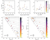Fig. 6.

Top row: pair-wise relationship between the fitting parameters, α₀, ν_char and γ in Eq. (1) shown for stars in our sample with spectroscopic parameters and sufficient CoRoT data for an accurate background fit. Bottom row: location of stars in the (spectroscopic) HR diagram as filled circles that have been colour-coded by the red-noise fit (Eq. (1)) parameters ν_char (left) and γ (right), with the size of each symbol corresponding to the fit parameter α₀. The location of stars with insufficient CoRoT data for an accurate background fit to the residual power density spectrum are shown as white triangles. Evolutionary tracks for representative masses (in units of M_⊙) from Ekström et al. (2012) are shown as solid grey lines, with the dashed grey line representing the ZAMS.

To compare the morphologies of the measured red noise profiles for the 18 stars with spectroscopic parameters and accurate background fits, we overplot them in Fig. 7 and colour-code each profile by each star’s spectroscopic luminosity. From inspection of Figs. 6 and 7 and of the individual summary figures of each star given in Appendix A, it is clear that the morphology of the observed red noise in upper-main sequence stars is quite diverse. This mirrors the diverse range of macroturbulence values found in the spectroscopy for stars on the upper-main sequence and is likely caused by the interplay of different dominant physical mechanisms causing the observed stochastic variability across the HR diagram – see the discussion from Simón-Díaz et al. (2017).

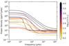Fig. 7.

Measured profiles of red noise determined from the power density spectra of CoRoT photometry for stars with known stellar parameters from spectroscopy and sufficient CoRoT data for an accurate background fit to the residual power density spectrum, which have been colour-coded by their spectroscopic luminosity.

6.2. A universal scaling law for granulation?

From the original work by Kjeldsen & Bedding (1995) the characteristic granulation frequency can be estimated from the scaling relation:

$\begin{matrix} ν_{gran} \propto \frac{c_{s}}{H_{p}} \propto M \cdot R^{- 2} \cdot T_{eff}^{- 1 / 2}, \end{matrix}$ $\begin{aligned} \nu _{\rm gran} \propto \frac{c_{\rm s}}{H_{\rm p}} \propto M \cdot R^{-2} \cdot T_{\rm eff}^{-1/2}, \end{aligned}$ (3)

where ν_gran is the granulation frequency, c_s is the sound speed, H_p is the pressure scale height, M is mass, R is radius, and T_eff is the effective temperature. The photometric amplitude of granulation is expected to inversely scale with the number of convective granules on a star’s surface, with the size of an individual granule being proportional to the pressure scale height H_p, whereas the granulation timescale is expected to scale with the ratio of the size and (sound) speed of a granule under the assumption of an ideal adiabatic gas (Stello et al. 2007; Huber et al. 2009).

As demonstrated by Kallinger et al. (2014) for thousands of pulsating solar-type and red giant stars, a tight correlation exists between ν_gran and the stellar parameters, such that the physics of surface convection in the Sun appears to adequately scale to stars on the red giant branch. From a Lorentzian fit to the power density spectra of the δ Sct stars HD 50844 and HD 174936, Kallinger & Matthews (2010) demonstrated that the red noise backgrounds in these stars were also consistent with those expected for granulation in A stars, but two evolved A stars are hardly representative of all A stars. If the use of this scaling relation for granulation is physically applicable to the sub-surface convection zones in high-mass stars, one would expect a similar smooth and tight correlation between the characteristic frequency and the stellar parameters.

To demonstrate the variance in the morphology of the observed red noise within our sample and specifically if the measured ν_char values depend on the stellar parameters as predicted by the characteristic granulation frequency given by Eq. (3), we place all 27 stars with spectroscopic parameters in Fig. 8. Similarly to Fig. 6, each circle in Fig. 8 represents a star with a reliable background fit whose size indicates the magnitude of α₀ and the colour indicates log₁₀(ℒ/ℒ_⊙). Stars with insufficient CoRoT data to accurately determine the fitting parameter γ are shown in Fig. 8 as white triangles. Our results for the previously studied δ Sct stars, HD 50844 and HD 174936, are consistent with those of Kallinger & Matthews (2010), such that the characteristic frequencies measured in the residual power density spectra of these A stars are similar to those expected for granulation. Other stars in our study, for example HD 174532, also have a red noise profiles that are consistent with granulation.

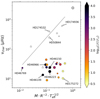Fig. 8.

Distribution of measured characteristic frequencies, ν_char, as a function of stellar parameters given in solar units. The grey line represents the granulation frequency scaled using Eq. (3) with the Sun’s location indicated by the ⊙ symbol. The circles have been colour-coded by a star’s spectroscopic luminosity and the size of the symbol is proportional to the fitting parameter, α₀. White triangles represent stars which may have insufficient CoRoT data for an accurate determination for the fitting parameter γ (cf. Eq. (3)).

However, the majority of our stars, which includes all of the main-sequence O and B stars and many of the main-sequence A and F stars, have characteristic frequencies that are approximately an order of magnitude smaller than the granulation frequency predicted by the scaling relation given in Eq. (3). If Eq. (3) is physically justified for main-sequence stars with masses M ≳ 2 M_⊙ then the observed low-frequency power excess is unlikely to be caused by granulation. Therefore, we conclude that granulation is not the cause of the low-frequency variability for the stars in the bottom-right corner of Fig. 8. On the other hand, if the red noise is caused by granulation, our results show that the scaling relation is not appropriate for stars with masses above 2 M_⊙.

Stellar winds are an important and possibly dominant cause of red noise in high-mass (M ≳ 15 M_⊙) stars. The dynamic, aspherical and clumpy winds of high-mass stars modulate the flux of a star as it rotates causing stochastic and non-periodic variability, yet the exact physical cause of wind clumping is not known but has been shown to originate within the stellar photosphere (Puls et al. 2006, 2008). Therefore as discussed by Aerts et al. (2018a), there is clearly a strong interplay and possible causal relationship between photospheric variability caused by pulsations and wind variability in high-mass stars. Although high-mass stars do not have convective envelopes whilst on the main sequence, their dynamic winds may explain the scatter and the lack of a tight correlation in the red noise morphology for upper main-sequence stars.

6.3. Photometric evidence of IGWs in early-type stars

Our CoRoT targets range in mass between 1.5 and 50 M_⊙, with all stars having characteristic frequencies that range approximately between 3 ≤ ν_char ≤ 630 μHz and 1.0 ≤ γ ≤ 17.0. However, when the stars with unreliable fits caused by insufficient data for removing unresolved pulsation modes are excluded, then the remaining 18 stars with available spectroscopic parameters and a significant low-frequency power excess have ν_char ≤ 50 μHz, which are not consistent with granulation as shown in Fig. 8.

As discussed in Sect. 3, the predicted morphology of IGWs is only weakly dependent on the stellar parameters for intermediate- and high-mass stars, such that we expect the dominant IGW frequencies to be in the approximate frequency range of 1 ≤ ν ≤ 3 d⁻¹ (11.6 ≤ ν ≤ 34.7 μHz), as shown in Fig. 1. Furthermore, numerical simulations of IGWs predict a low-frequency power excess with a frequency exponent between −1 and −3 dependent on the rotation rate and interior differential rotation profile of a star (Rogers et al. 2013; Rogers 2015). A histogram of the γ values of the 18 stars with reliable background fits is shown in Fig. 9, which is colour-coded by each star’s spectroscopic effective luminosity, and demonstrates that almost all stars have a low-frequency power excess with γ ≤ 5 as predicted by numerical simulations of IGWs (Rogers et al. 2013; Rogers 2015).

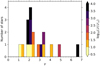Fig. 9.

Histogram of fitting parameter γ (cf. Eq. (1)) for all stars with spectroscopic parameters and sufficient CoRoT data for an accurate background fit to the residual power density spectrum.

Our results show that the majority of the stars in our sample have a low-frequency power excess, albeit with different amplitudes, which is consistent with the predictions of numerical simulations of a spectrum of IGWs with multiple values of ℓ and m (Rogers et al. 2013; Rogers 2015). Therefore, from the grouping stars in Fig. 8, which implies that granulation is unlikely to be responsible, and because the distribution of the frequency exponent, γ, agrees with predictions by numerical simulations of IGWs, we conclude that the low-frequency variability in our sample of O, B, A and F stars is caused by IGWs. This is the only physical mechanism that can cause photometric red noise across the whole mass range, since all stars with a convective core are expected to excite IGWs (Samadi et al. 2010; Shiode et al. 2013; Rogers et al. 2013; Rogers 2015). Furthermore, this conclusion is supported by the fact that not all stars in our sample are expected to have red noise caused by stellar winds, granulation or sub-surface convection (Samadi et al. 2010; Cantiello et al. 2009a).

There is an interesting outlier in the HR diagrams shown in Fig. 6 and the measured characteristic frequency distribution shown in Fig. 8, which is the blue supergiant HD 46769. This star has a relatively low surface gravity of log g < 3.0, such that this post-main sequence star likely has a surface convection zone. The measured characteristic frequency in HD 46769 lies close to the expected granulation frequency in Fig. 8. As stars evolve off the main sequence, they will generally move to the left in Fig. 8 because of the large increase in radius. Moreover, they will develop an outer convection zone that becomes deeper as the star evolves further, which could plausibly cause granulation. Therefore, assuming that the granulation scaling relation holds for high-mass stars, it is plausible that the red noise detected in HD 46769 is caused by granulation.

The blue supergiants HD 188209 (Aerts et al. 2017a) and HD 91316 (Aerts et al. 2018a) are known to have large values of macroturbulence, and low-frequency variability of order a few mmag. Conversely, the blue supergiant HD 46769 studied using spectroscopy by Aerts et al. (2013), was found to have an unusually low macroturbulence of v_macro < 10 km s⁻¹. The low-amplitude red noise of order a few μmag (i.e. α₀ ≃ 35 ppm²/μHz) that we found in the CoRoT photometry of HD 46769 implies a common physical cause for these two observables and warrants further study (e.g. Simón-Díaz et al. 2017). This work emphasises the complementary nature of studying stochastic low-frequency variability in blue supergiants with both photometry and spectroscopy. In a future paper, we will explore the complementarity of studying spectroscopic macroturbulence and photometric red noise using a large sample of blue supergiants observed by Kepler and K2.

7. Future prospects with TESS

In the near future, we will be able to further populate our HR diagram and characterise the morphology of IGWs in massive stars by including stars observed by the TESS mission (Ricker et al. 2015), which was launched on 18 April 2018. To achieve its primary goal of finding transiting exoplanets around the brightest stars in the sky, TESS has a wavelength passband that covers 6000−10 000 Å, which is redder than the passbands of the CoRoT and Kepler missions (Auvergne et al. 2009; Borucki et al. 2010). Eventually, TESS will observe a large fraction of the sky, with a cadence of 30 min and observing runs that last from 27 d up to 1 yr in the continuous viewing zones (CVZs) near the ecliptic polar regions (Ricker et al. 2015). Although TESS is optimised to study cool stars, asteroseismology of many different types of stars will be possible.

The exciting prospect of TESS for upper-main sequence stars is that it will observe many more O and B stars compared to any other previous space-based telescope. Furthermore, TESS will provide continuous high-quality light curves for hundreds of early-O to late-B stars in its southern CVZ. We plot the distribution of these stars in the TESS southern-CVZ in Fig. 10, with each circle colour-coded by spectral type and the size denoting the V-band magnitude, which ranges between 5 ≤ V ≤ 13 mag.

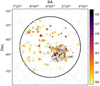Fig. 10.

Location of the O and B stars that TESS is observing for 1 yr in its southern continuous viewing zone, with the colour-scale indicating the spectral type and the size of the symbol indicating the V-band magnitude.

However, an important consequence of the TESS wavelength passband for massive stars is the photometric suppression of a star’s intrinsic variability. This is illustrated in Fig. 11, in which the Planck blackbody function for a representative T_eff = 10 000 K star is shown. The simulated flux perturbations caused by pulsations at the surface of a star perturb the T_eff to slightly hotter and cooler values during a pulsation cycle, which are represented by the blue and red solid lines in Fig. 11, respectively. The flux variations, dF/F, caused by pulsations can be approximated as the difference between the area beneath the blackbody curve at the temperature maximum and minimum within the wavelength range imposed by an instrument’s passband.

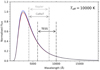Fig. 11.

Normalised Planck blackbody function for a T_eff = 10 000 K star, and hotter and cooler perturbations caused by pulsations are shown as black, blue and red solid lines, respectively. The approximate wavelength ranges for TESS, CoRoT and Kepler passbands are shown as dashed, dash-dot and dotted lines, respectively.

For a first-order estimate of the expected TESS pulsation amplitude suppression factor for massive stars, we use the wavelength range for which the quantum efficiency of an instrument’s CCD is above 50 percent, which corresponds to an approximate wavelength of 4100−8500 Å for CoRoT, with a similar range of 4300−8300 Å for Kepler since both instruments cover the visible wavelength range, and 6000–10 000 Å for TESS. Our calculations for the ratio of TESS and CoRoT, and TESS and Kepler instruments yield an estimate of the photometric amplitudes that TESS will observe relative to the CoRoT and Kepler telescopes, respectively. Individual values for representative effective temperatures are given in Table 3 but these values include large assumptions and are only given for illustrative purposes. Of course, the true test of these estimations will come when TESS observes stars that have previously been observed by CoRoT and Kepler, and the ratios can be measured directly – see Bowman et al. (2015) for an example.

Table 3.

Expected TESS pulsation amplitudes for high-mass stars expressed as a relative percentage compared to the CoRoT and Kepler passbands.

Taking the example of an early-F star with T_eff = 7000 K star, photometric amplitudes will be approximately 50 percent lower than those observed by CoRoT and Kepler – a pulsation mode amplitude of 1 mmag in a star will be approximately 0.5 mmag as observed by TESS because of the redder passband. For a more massive, and hence hotter, star such as an O star with an effective temperature of T_eff = 30 000 K, the suppression factor is larger and hence the ratios A_TESS/A_CoRoT and A_TESS/A_Kepler become smaller because the peak of the Blackbody function is at bluer wavelengths. Therefore, the observational signatures of pulsations in massive stars, whether they are coherent or damped pulsation modes, will be suppressed in amplitude because of the TESS passband. Hence, this bias towards detecting photometric variability in cooler stars should be taken into account when studying the variability of massive stars, as redder passbands underestimate the true photometric variability.

8. Conclusions

Previous studies that looked at individual or small samples of massive stars (i.e. M ≳ 15 M_⊙) have noted the presence of astrophysical red noise in the photometry of these stars (e.g. Blomme et al. 2011). Typically, the origin of a low-frequency power excess in massive stars has been interpreted as being caused by a dynamic stellar wind, granulation or sub-surface convection, or more recently IGWs. All of these physical explanations are plausible for massive stars, but are difficult to disentangle especially because they are not mutually exclusive for an individual star. However, recent studies have begun to unravel the different mechanisms causing stochastic variability that may be dominant in different mass regimes and at different evolutionary stages for massive stars (e.g. Aerts et al. 2017a, 2018a; Simón-Díaz et al. 2018).

In our study using CoRoT photometry, we demonstrate that the physical interpretation of stochastic variability in high-mass stars requires a long and continuous time series to provide the necessary frequency resolution to remove coherent modes via iterative pre-whitening. We have confronted the 2D numerical simulations of IGWs from Rogers et al. (2013) with photometry of numerous O, B, A and F stars. We parameterise the low-frequency power excess in these stars and demonstrate the diverse range in the morphology of their stochastic low-frequency variability. For some of the A and F stars in our sample, we find that the morphology of the photometric red noise is consistent with that expected from the granulation scaling relation (e.g. Kallinger & Matthews 2010). Yet this is certainly not the case for all A and F stars in our sample. Furthermore, we also demonstrate that the red noise in post-main sequence stars is also consistent with granulation including the blue supergiant HD 46769, which is expected to have a convective envelope.

The majority of the stars in our study required a significantly different parametrisation of the low-frequency power excess, which were not compatible with their expected characteristic granulation frequencies. As demonstrated in Fig. 7, the diversity in the observed red noise profiles is clearly large for the stars in our sample. Yet, the measured characteristic frequencies in the majority of our stars are between 1 ≤ ν ≤ 4 d⁻¹ (11.6 ≤ ν ≤ 46.3 μHz), which is approximately an order of magnitude smaller than expected for granulation and coincides within the frequency range of where the amplitudes of IGWs are predicted to be at their highest (Rogers et al. 2013; Rogers 2015).

We demonstrate that the peaks in the residual background spectra are variable in amplitude and frequency, and have amplitudes that are of order 10 μmag in A and F stars and increase to a few hundred μmag for O and B stars. These values are comparable as those predicted by Shiode et al. (2013), and are similarly correlated with stellar mass. Hence we find the first observational evidence of relationship between the photometric amplitudes of IGWs and stellar mass for main-sequence stars. This further supports the interpretation of IGWs as an explanation for the observed photometric red noise, since the larger convective cores in massive stars are predicted to excite IGWs with larger amplitudes (Shiode et al. 2013; Aerts & Rogers 2015).

Recent theoretical work and 3D numerical simulations of IGWs triggered by turbulent convection in a Cartesian model by Couston et al. (2018) predict the same power-law frequency spectrum for IGWs as Lecoanet & Quataert (2013), with a frequency exponent of −13/2 (corresponding to γ = 6.5). This is steeper than the power-law predicted by 3D simulations of core convection in a 3 M_⊙ star by Edelmann et al. (2018). The latter simulations take into account the spherical configuration, as well as an appropriate density stratification from a realistic stellar model. These simulations rather predict an IGW frequency spectrum with a frequency exponent between −1.5 and −3 (i.e. γ ∈ [1.5, 3]), which is similar to other simulations of core convection by Rogers et al. (2013) and Augustson et al. (2016). Our analysis of CoRoT stars with a convective core leads to γ ≤ 5 for the majority of well-characterised stars.

A theoretically-predicted power-law excess caused by wind instabilities in the massive O stars HD 46150, HD 46223 and HD 46966 has also recently been investigated by Krtička & Feldmeier (2018). Whilst wind instabilities could potentially provide an plausible explanation for the most massive (i.e. M > 15 M_⊙) stars in our sample, it is not a physical explanation for the similar low-frequency excess observed in intermediate-mass B, A and F stars.

In this work, we have demonstrated that the morphology of the low-frequency power excess observed in many O, B, A, and F stars, which we have parametrised using Eq. (1), is not consistent with granulation (cf. Fig. 8). Furthermore, as demonstrated in Fig. 9, the majority of stars required γ ≤ 5, which is consistent with the frequency exponent predictions of an entire frequency spectrum of IGWs of various length scales (Rogers et al. 2013; Rogers 2015; Edelmann et al. 2018). These observations are useful for constraining the driving and damping processes in numerical simulations of core convection and IGWs for various stellar masses and stages of stellar evolution.

Regardless of the interpretation of the low-frequency power excess found in many stars in our study, we provide valuable constraints on the maximum amplitude of the background IGW spectrum across the HR diagram. Guided by the results of the present study that main-sequence massive stars represent the best targets for detecting IGWs, we can probe the differences between observations and the frequency spectra predicted by simulations of IGWs and sub-surface granulation. Our current study represents an important ensemble characterisation of variability in massive stars, which demonstrates the diverse range of physical phenomena at work in early-type stars. We are currently limited to a few dozen early-type stars by CoRoT, which were only observed for a relatively short time span, until TESS observations of O and B stars become available. In a subsequent paper, we will further populate our asteroseismic HR diagram with many more O and B stars using photometry from the K2 and TESS missions. The future of asteroseismology of massive O and B stars is bright, with our study representing a necessary first-step in understanding the parameter space of stochastic variability in early-type stars.

¹

We note that the conversion between flux variations expressed in μmag and ppm is 2.5 log₁₀(e) = 1.08574.

²

We note that the conversion between frequency expressed in d⁻¹ and μHz is $\frac{625}{54} = 11.57407$ $\frac{625}{54} = 11.57407$ .

³

We note that the difference in the model parameters from our study and that of Blomme et al. (2011) is caused by the difference in units.

Acknowledgments

The authors thank the CoRoT science team for the excellent data and the referee for the useful comments that improved the manuscript. D.M.B. is grateful to Dr. Kelly Hambleton for useful discussions. The CoRoT space mission was developed and operated by the French space agency CNES, with participation of ESA’s RSSD and Science Programmes, Austria, Belgium, Brazil, Germany, and Spain. This research has made use of the SIMBAD database, operated at CDS, Strasbourg, France; the SAO/NASA Astrophysics Data System; and the VizieR catalogue access tool, CDS, Strasbourg, France. The research leading to these results has received funding from the European Research Council (ERC) under the European Union’s Horizon 2020 research and innovation programme (grant agreement N°670519: MAMSIE). S.S.-D. acknowledges financial support from the Spanish Ministry of Economy and Competitiveness (MINECO) through grants AYA2015-68012-C2-1 and Severo Ochoa SEV-2015-0548, and grant ProID2017010115 from the Gobierno de Canarias. Support for this research was provided by STFC grant ST/L005549/1 and NASA grant NNX17AB92G. T.V.R. gratefully acknowledges support from the Australian Research Council, and from the Danish National Research Foundation (Grant DNRF106) through its funding for the Stellar Astrophysics Centre (SAC).

References

Abt, H. A., & Biggs, E. S. 1972, Bibliography of Stellar Radial Velocities (New York: Latham Process Corp) [Google Scholar]
Abt, H. A., & Cardona, O. 1984, ApJ, 285, 190 [NASA ADS] [CrossRef] [Google Scholar]
Abt, H. A., Levato, H., & Grosso, M. 2002, ApJ, 573, 359 [NASA ADS] [CrossRef] [Google Scholar]
Adelman, S. J. 2001, A&A, 367, 297 [NASA ADS] [CrossRef] [EDP Sciences] [Google Scholar]
Aerts, C., & Rogers, T. M. 2015, ApJ, 806, L33 [NASA ADS] [CrossRef] [Google Scholar]
Aerts, C., Puls, J., Godart, M., & Dupret, M.-A. 2009, A&A, 508, 409 [NASA ADS] [CrossRef] [EDP Sciences] [Google Scholar]
Aerts, C., Christensen-Dalsgaard, J., & Kurtz, D. W. 2010, Asteroseismology (Springer) [Google Scholar]
Aerts, C., Briquet, M., Degroote, P., Thoul, A., & van Hoolst, T. 2011, A&A, 534, A98 [NASA ADS] [CrossRef] [EDP Sciences] [Google Scholar]
Aerts, C., Simón-Díaz, S., Catala, C., et al. 2013, A&A, 557, A114 [NASA ADS] [CrossRef] [EDP Sciences] [Google Scholar]
Aerts, C., Simón-Díaz, S., Groot, P. J., & Degroote, P. 2014, A&A, 569, A118 [NASA ADS] [CrossRef] [EDP Sciences] [Google Scholar]
Aerts, C., Símon-Díaz, S., Bloemen, S., et al. 2017a, A&A, 602, A32 [NASA ADS] [CrossRef] [EDP Sciences] [Google Scholar]
Aerts, C., Van Reeth, T., & Tkachenko, A. 2017b, ApJ, 847, L7 [NASA ADS] [CrossRef] [Google Scholar]
Aerts, C., Bowman, D. M., Símon-Díaz, S., et al. 2018a, MNRAS, 476, 1234 [NASA ADS] [CrossRef] [Google Scholar]
Aerts, C., Mathis, S., & Rogers, T. 2018b, ARA&A, submitted [arXiv:1809.07779] [Google Scholar]
Ahmed, A., & Sigut, T. A. A. 2017, MNRAS, 471, 3398 [NASA ADS] [CrossRef] [Google Scholar]
Aldoretta, E. J., Caballero-Nieves, S. M., Gies, D. R., et al. 2015, AJ, 149, 26 [NASA ADS] [CrossRef] [Google Scholar]
Appourchaux, T. 2003, Ap&SS, 284, 109 [NASA ADS] [CrossRef] [Google Scholar]
Appourchaux, T. 2008, Astron. Nachr., 329, 485 [NASA ADS] [CrossRef] [Google Scholar]
Appourchaux, T., Gizon, L., & Rabello-Soares, M.-C. 1998, A&AS, 132, 107 [NASA ADS] [CrossRef] [EDP Sciences] [Google Scholar]
Appourchaux, T., Michel, E., Auvergne, M., et al. 2008, A&A, 488, 705 [NASA ADS] [CrossRef] [EDP Sciences] [Google Scholar]
Augustson, K. C., Brun, A. S., & Toomre, J. 2016, ApJ, 829, 92 [NASA ADS] [CrossRef] [Google Scholar]
Auvergne, M., Bodin, P., Boisnard, L., et al. 2009, A&A, 506, 411 [NASA ADS] [CrossRef] [EDP Sciences] [Google Scholar]
Bailer-Jones, C. A. L. 2011, MNRAS, 411, 435 [NASA ADS] [CrossRef] [Google Scholar]
Balona, L. A. 1992, MNRAS, 254, 403 [NASA ADS] [CrossRef] [Google Scholar]
Balona, L. A. 2014, MNRAS, 439, 3453 [NASA ADS] [CrossRef] [Google Scholar]
Barceló Forteza, S., Roca Cortés, T., García Hernández, A., & García, R. A. 2017, A&A, 601, A57 [NASA ADS] [CrossRef] [EDP Sciences] [Google Scholar]
Baumgardt, H., Dettbarn, C., & Wielen, R. 2000, A&AS, 146, 251 [NASA ADS] [CrossRef] [EDP Sciences] [Google Scholar]
Belkacem, K., Dupret, M. A., & Noels, A. 2010, A&A, 510, A6 [NASA ADS] [CrossRef] [EDP Sciences] [Google Scholar]
Benomar, O., Appourchaux, T., & Baudin, F. 2009, A&A, 506, 15 [NASA ADS] [CrossRef] [EDP Sciences] [Google Scholar]
Blomme, R., Mahy, L., Catala, C., et al. 2011, A&A, 533, A4 [NASA ADS] [CrossRef] [EDP Sciences] [Google Scholar]
Bonatto, C., & Bica, E. 2009, MNRAS, 394, 2127 [NASA ADS] [CrossRef] [Google Scholar]
Borucki, W. J., Koch, D., Basri, G., et al. 2010, Science, 327, 977 [NASA ADS] [CrossRef] [PubMed] [Google Scholar]
Bowman, D. M. 2016, PhD Thesis Jeremiah Horrocks Institute, University of Central Lancashire, Preston, UK [Google Scholar]
Bowman, D. M. 2017, Amplitude Modulation of Pulsation Modes in Delta Scuti Stars (Springer International Publishing) [CrossRef] [Google Scholar]
Bowman, D. M., & Kurtz, D. W. 2018, MNRAS, 476, 3169 [NASA ADS] [CrossRef] [Google Scholar]
Bowman, D. M., Holdsworth, D. L., & Kurtz, D. W. 2015, MNRAS, 449, 1004 [NASA ADS] [CrossRef] [Google Scholar]
Bowman, D. M., Kurtz, D. W., Breger, M., Murphy, S. J., & Holdsworth, D. L. 2016, MNRAS, 460, 1970 [NASA ADS] [CrossRef] [Google Scholar]
Bragança, G. A., Daflon, S., Cunha, K., et al. 2012, AJ, 144, 130 [NASA ADS] [CrossRef] [Google Scholar]
Breger, M. 2000, MNRAS, 313, 129 [CrossRef] [Google Scholar]
Breger, M., Stich, J., Garrido, R., et al. 1993, A&A, 271, 482 [NASA ADS] [Google Scholar]
Breger, M., Pamyatnykh, A. A., Zima, W., et al. 2002, MNRAS, 336, 249 [NASA ADS] [CrossRef] [Google Scholar]
Breger, M., Rodler, F., Pretorius, M. L., et al. 2004, A&A, 419, 695 [NASA ADS] [CrossRef] [EDP Sciences] [Google Scholar]
Briquet, M., Aerts, C., Baglin, A., et al. 2011, A&A, 527, A112 [NASA ADS] [CrossRef] [EDP Sciences] [Google Scholar]
Browning, M. K., Brun, A. S., & Toomre, J. 2004, ApJ, 601, 512 [NASA ADS] [CrossRef] [Google Scholar]
Buysschaert, B., Aerts, C., Bloemen, S., et al. 2015, MNRAS, 453, 89 [NASA ADS] [CrossRef] [Google Scholar]
Buysschaert, B., Neiner, C., Richardson, N. D., et al. 2017, A&A, 602, A91 [NASA ADS] [CrossRef] [EDP Sciences] [Google Scholar]
Buysschaert, B., Aerts, C., Bowman, D. M., et al. 2018, A&A, 616, A148 [NASA ADS] [CrossRef] [EDP Sciences] [Google Scholar]
Cantiello, M., Langer, N., Brott, I., et al. 2009a, A&A, 499, 279 [NASA ADS] [CrossRef] [EDP Sciences] [Google Scholar]
Cantiello, M., Langer, N., Brott, I., et al. 2009b, Commun. Asteroseismol., 158, 61 [NASA ADS] [Google Scholar]
Cantiello, M., Mankovich, C., Bildsten, L., Christensen-Dalsgaard, J., & Paxton, B. 2014, ApJ, 788, 93 [NASA ADS] [CrossRef] [Google Scholar]
Casagrande, L., Schönrich, R., Asplund, M., et al. 2011, A&A, 530, A138 [NASA ADS] [CrossRef] [EDP Sciences] [Google Scholar]
Castelli, F., & Hubrig, S. 2004, A&A, 425, 263 [NASA ADS] [CrossRef] [EDP Sciences] [Google Scholar]
Chaplin, W. J., & Miglio, A. 2013, ARA&A, 51, 353 [NASA ADS] [CrossRef] [Google Scholar]
Charbonnel, C., & Talon, S. 2005, Science, 309, 2189 [NASA ADS] [CrossRef] [PubMed] [Google Scholar]
Charbonnel, C., Decressin, T., Amard, L., Palacios, A., & Talon, S. 2013, A&A, 554, A40 [NASA ADS] [CrossRef] [EDP Sciences] [Google Scholar]
Chini, R., Hoffmeister, V. H., Nasseri, A., Stahl, O., & Zinnecker, H. 2012, MNRAS, 424, 1925 [NASA ADS] [CrossRef] [Google Scholar]
Claria, J. J. 1972, A&A, 19, 303 [NASA ADS] [Google Scholar]
Couston, L.-A., Lecoanet, D., Favier, B., & Le Bars, M. 2018, J. Fluid Mech., 854, R3 [CrossRef] [Google Scholar]
David, T. J., & Hillenbrand, L. A. 2015, ApJ, 804, 146 [NASA ADS] [CrossRef] [Google Scholar]
Davies, G. R., Silva Aguirre, V., Bedding, T. R., et al. 2016, MNRAS, 456, 2183 [NASA ADS] [CrossRef] [Google Scholar]
de Bruijne, J. H. J., & Eilers, A.-C. 2012, A&A, 546, A61 [NASA ADS] [CrossRef] [EDP Sciences] [Google Scholar]
Degroote, P., Briquet, M., Catala, C., et al. 2009, A&A, 506, 111 [NASA ADS] [CrossRef] [EDP Sciences] [Google Scholar]
Degroote, P., Aerts, C., Baglin, A., et al. 2010a, Nature, 464, 259 [NASA ADS] [CrossRef] [PubMed] [Google Scholar]
Degroote, P., Aerts, C., Samadi, R., et al. 2010b, Astron. Nachr., 331, 1065 [NASA ADS] [CrossRef] [Google Scholar]
Degroote, P., Briquet, M., Auvergne, M., et al. 2010c, A&A, 519, A38 [NASA ADS] [CrossRef] [EDP Sciences] [Google Scholar]
Degroote, P., Acke, B., Samadi, R., et al. 2011, A&A, 536, A82 [NASA ADS] [CrossRef] [EDP Sciences] [Google Scholar]
Dolez, N., Vauclair, S., Michel, E., et al. 2009, A&A, 506, 159 [NASA ADS] [CrossRef] [EDP Sciences] [Google Scholar]
Dolk, L., Wahlgren, G. M., Lundberg, H., et al. 2002, A&A, 385, 111 [NASA ADS] [CrossRef] [EDP Sciences] [Google Scholar]
Dommanget, J., & Nys, O. 2000, A&A, 363, 991 [NASA ADS] [Google Scholar]
Douglass, G. G., Mason, B. D., Germain, M. E., & Worley, C. E. 1999, AJ, 118, 1395 [NASA ADS] [CrossRef] [Google Scholar]
Dziembowski, W. A., & Pamyatnykh, A. A. 2008, MNRAS, 385, 2061 [NASA ADS] [CrossRef] [Google Scholar]
Edelmann, P. V. F., Ratnasingam, R. P., Pedersen, M. G., et al. 2018, ApJ, submitted [Google Scholar]
Eggenberger, P., Lagarde, N., Miglio, A., et al. 2017, A&A, 599, A18 [NASA ADS] [CrossRef] [EDP Sciences] [Google Scholar]
Eggleton, P. P., & Tokovinin, A. A. 2008, MNRAS, 389, 869 [NASA ADS] [CrossRef] [Google Scholar]
Ekström, S., Georgy, C., Eggenberger, P., et al. 2012, A&A, 537, A146 [NASA ADS] [CrossRef] [EDP Sciences] [Google Scholar]
Fabricius, C., Høg, E., Makarov, V. V., et al. 2002, A&A, 384, 180 [NASA ADS] [CrossRef] [EDP Sciences] [Google Scholar]
Foreman-Mackey, D., Hogg, D. W., Lang, D., & Goodman, J. 2013, PASP, 125, 306 [CrossRef] [Google Scholar]
Fossati, L., Castro, N., Schöller, M., et al. 2015, A&A, 582, A45 [NASA ADS] [CrossRef] [EDP Sciences] [Google Scholar]
Fox Machado, L., Michel, R., Álvarez, M., et al. 2008, Commun. Asteroseismol., 153, 20 [NASA ADS] [CrossRef] [Google Scholar]
Fox Machado, L., Alvarez, M., Michel, R., et al. 2010, New Astron., 15, 397 [NASA ADS] [CrossRef] [Google Scholar]
Frankowski, A., Jancart, S., & Jorissen, A. 2007, A&A, 464, 377 [NASA ADS] [CrossRef] [EDP Sciences] [Google Scholar]
Frémat, Y., Neiner, C., Hubert, A.-M., et al. 2006, A&A, 451, 1053 [NASA ADS] [CrossRef] [EDP Sciences] [Google Scholar]
Fuller, J., Lecoanet, D., Cantiello, M., & Brown, B. 2014, ApJ, 796, 17 [Google Scholar]
Fuller, J., Cantiello, M., Lecoanet, D., & Quataert, E. 2015, ApJ, 810, 101 [NASA ADS] [CrossRef] [Google Scholar]
Fullerton, A. W. 1990, PhD Thesis, Toronto Univ. (Ontario, Canada) [Google Scholar]
Fullerton, A. W., Gies, D. R., & Bolton, C. T. 1996, ApJS, 103, 475 [NASA ADS] [CrossRef] [Google Scholar]
Fullerton, A. W., Massa, D. L., & Prinja, R. K. 2006, ApJ, 637, 1025 [NASA ADS] [CrossRef] [Google Scholar]
García Hernández, A., Moya, A., Michel, E., et al. 2009, A&A, 506, 79 [NASA ADS] [CrossRef] [EDP Sciences] [Google Scholar]
García Hernández, A., Moya, A., Michel, E., et al. 2013, A&A, 559, A63 [NASA ADS] [CrossRef] [EDP Sciences] [Google Scholar]
Gaulme, P., Appourchaux, T., & Boumier, P. 2009, A&A, 506, 7 [NASA ADS] [CrossRef] [EDP Sciences] [Google Scholar]
Gebran, M., Farah, W., Paletou, F., Monier, R., & Watson, V. 2016, A&A, 589, A83 [NASA ADS] [CrossRef] [EDP Sciences] [Google Scholar]
Gelman, A., & Rubin, D. B. 1992, Stat. Sci., 7, 457 [Google Scholar]
Germain, M. E., Douglass, G. G., & Worley, C. E. 1999, AJ, 117, 2511 [NASA ADS] [CrossRef] [Google Scholar]
Ghazaryan, S., Alecian, G., & Harutyunian, H. 2013, MNRAS, 435, 1852 [NASA ADS] [CrossRef] [Google Scholar]
Godart, M., Simón-Díaz, S., Herrero, A., et al. 2017, A&A, 597, A23 [NASA ADS] [CrossRef] [EDP Sciences] [Google Scholar]
Gontcharov, G. A. 2006, Astron. Lett., 32, 759 [NASA ADS] [CrossRef] [Google Scholar]
Grassitelli, L., Fossati, L., Simón-Diáz, S., et al. 2015, ApJ, 808, L31 [NASA ADS] [CrossRef] [Google Scholar]
Gruberbauer, M., Kallinger, T., Weiss, W. W., & Guenther, D. B. 2009, A&A, 506, 1043 [NASA ADS] [CrossRef] [EDP Sciences] [Google Scholar]
Grunhut, J. H., Wade, G. A., Neiner, C., et al. 2017, MNRAS, 465, 2432 [NASA ADS] [CrossRef] [Google Scholar]
Gutiérrez-Soto, J., Fabregat, J., Suso, J., et al. 2007, A&A, 476, 927 [NASA ADS] [CrossRef] [EDP Sciences] [Google Scholar]
Gutiérrez-Soto, J., Neiner, C., Fabregat, J., et al. 2011, in Active OB Stars: Structure, Evolution, Mass Loss, and Critical Limits, eds. C. Neiner, G. Wade, G. Meynet, & G. Peters, IAU Symp., 272, 451 [NASA ADS] [Google Scholar]
Hambleton, K. M. 2016, PhD Thesis, Jeremiah Horrocks Institute, University of Central Lancashire, UK [Google Scholar]
Hambleton, K., Fuller, J., Thompson, S., et al. 2018, MNRAS, 473, 5165 [NASA ADS] [CrossRef] [Google Scholar]
Handberg, R., & Campante, T. L. 2011, A&A, 527, A56 [NASA ADS] [CrossRef] [EDP Sciences] [Google Scholar]
Handler, G., Matthews, J. M., Eaton, J. A., et al. 2009, ApJ, 698, L56 [NASA ADS] [CrossRef] [Google Scholar]
Harvey, J. 1985, in Future Missions in Solar, Heliospheric & Space Plasma Physics, eds. E. Rolfe, & B. Battrick, ESA SP, 235 [Google Scholar]
Hauck, B., & Mermilliod, M. 1998, A&AS, 129, 431 [NASA ADS] [CrossRef] [EDP Sciences] [Google Scholar]
Heger, A., Langer, N., & Woosley, S. E. 2000, ApJ, 528, 368 [NASA ADS] [CrossRef] [Google Scholar]
Hekker, S., & Ball, W. H. 2014, A&A, 564, A105 [NASA ADS] [CrossRef] [EDP Sciences] [Google Scholar]
Hekker, S., & Christensen-Dalsgaard, J. 2017, A&ARv, 25, 1 [NASA ADS] [CrossRef] [EDP Sciences] [Google Scholar]
Hensberge, H., Pavlovski, K., & Verschueren, W. 2000, A&A, 358, 553 [NASA ADS] [Google Scholar]
Hohle, M. M., Neuhäuser, R., & Schutz, B. F. 2010, Astron. Nachr., 331, 349 [NASA ADS] [CrossRef] [Google Scholar]
Holmberg, J., Nordström, B., & Andersen, J. 2009, A&A, 501, 941 [NASA ADS] [CrossRef] [EDP Sciences] [Google Scholar]
Houk, N., & Swift, C. 1999, Michigan Catalogue of Two-dimensional Spectral Types for the HD Stars (University of Michigan), 5 [Google Scholar]
Howarth, I. D., Goss, K. J. F., Stevens, I. R., Chaplin, W. J., & Elsworth, Y. 2014, MNRAS, 440, 1674 [NASA ADS] [CrossRef] [Google Scholar]
Howell, S. B., Sobeck, C., Haas, M., et al. 2014, PASP, 126, 398 [NASA ADS] [CrossRef] [Google Scholar]
Huber, D., Stello, D., Bedding, T. R., et al. 2009, Commun. Asteroseismol., 160, 74 [NASA ADS] [CrossRef] [Google Scholar]
Hubrig, S., Castelli, F., Mathys, G., & Wahlgren, G. M. 2001, in Magnetic Fields Across the Hertzsprung-Russell Diagram, eds. G. Mathys, S. K. Solanki, & D. T. Wickramasinghe, ASP Conf. Ser., 248, 387 [NASA ADS] [Google Scholar]
Iijima, T., & Ishida, K. 1978, PASJ, 30, 657 [NASA ADS] [Google Scholar]
Johnston, C., Buysschaert, B., Tkachenko, A., Aerts, C., & Neiner, C. 2017, MNRAS, 469, L118 [NASA ADS] [CrossRef] [Google Scholar]
Kallinger, T., & Matthews, J. M. 2010, ApJ, 711, L35 [NASA ADS] [CrossRef] [Google Scholar]
Kallinger, T., De Ridder, J., Hekker, S., et al. 2014, A&A, 570, A41 [NASA ADS] [CrossRef] [EDP Sciences] [Google Scholar]
Kjeldsen, H., & Bedding, T. R. 1995, A&A, 293, 87 [NASA ADS] [Google Scholar]
Kochukhov, O., Johnston, C., Alecian, E., & Wade, G. A. 2018, MNRAS, 478, 1749 [NASA ADS] [CrossRef] [Google Scholar]
Koen, C., & Eyer, L. 2002, MNRAS, 331, 45 [NASA ADS] [CrossRef] [Google Scholar]
Krtička, J., & Feldmeier, A. 2018, A&A, 617, A121 [NASA ADS] [CrossRef] [EDP Sciences] [Google Scholar]
Kurtz, D. W., Cameron, C., Cunha, M. S., et al. 2005, MNRAS, 358, 651 [NASA ADS] [CrossRef] [Google Scholar]
Kurtz, D. W., Saio, H., Takata, M., et al. 2014, MNRAS, 444, 102 [NASA ADS] [CrossRef] [Google Scholar]
Kurtz, D. W., Shibahashi, H., Murphy, S. J., Bedding, T. R., & Bowman, D. M. 2015, MNRAS, 450, 3015 [NASA ADS] [CrossRef] [Google Scholar]
Landstreet, J. D., Kupka, F., Ford, H. A., et al. 2009, A&A, 503, 973 [NASA ADS] [CrossRef] [EDP Sciences] [Google Scholar]
Lecoanet, D., & Quataert, E. 2013, MNRAS, 430, 2363 [NASA ADS] [CrossRef] [Google Scholar]
Lecoanet, D., Vasil, G. M., Fuller, J., Cantiello, M., & Burns, K. J. 2017, MNRAS, 466, 2181 [NASA ADS] [CrossRef] [Google Scholar]
Lee, U., Neiner, C., & Mathis, S. 2014, MNRAS, 443, 1515 [NASA ADS] [CrossRef] [Google Scholar]
Lefever, K., Puls, J., & Aerts, C. 2007, A&A, 463, 1093 [NASA ADS] [CrossRef] [EDP Sciences] [Google Scholar]
Lefever, K., Puls, J., Morel, T., et al. 2010, A&A, 515, A74 [NASA ADS] [CrossRef] [EDP Sciences] [Google Scholar]
Lefèvre, L., Marchenko, S. V., Moffat, A. F. J., & Acker, A. 2009, A&A, 507, 1141 [NASA ADS] [CrossRef] [EDP Sciences] [Google Scholar]
Levato, H., & Malaroda, S. 1974, AJ, 79, 890 [NASA ADS] [CrossRef] [Google Scholar]
Liu, T., Janes, K. A., & Bania, T. M. 1989, AJ, 98, 626 [NASA ADS] [CrossRef] [Google Scholar]
Liu, C.-Y., Doressoundiram, A., Roques, F., et al. 2015, MNRAS, 446, 932 [NASA ADS] [CrossRef] [Google Scholar]
Lyubimkov, L. S., Lambert, D. L., Rachkovskaya, T. M., et al. 2000, MNRAS, 316, 19 [NASA ADS] [CrossRef] [Google Scholar]
Lyubimkov, L. S., Rachkovskaya, T. M., Rostopchin, S. I., & Lambert, D. L. 2002, MNRAS, 333, 9 [NASA ADS] [CrossRef] [Google Scholar]
Lyubimkov, L. S., Rostopchin, S. I., Rachkovskaya, T. M., Poklad, D. B., & Lambert, D. L. 2005, MNRAS, 358, 193 [NASA ADS] [CrossRef] [Google Scholar]
Lyubimkov, L. S., Lambert, D. L., Poklad, D. B., Rachkovskaya, T. M., & Rostopchin, S. I. 2013, MNRAS, 428, 3497 [NASA ADS] [Google Scholar]
Maeder, A. 2009, Physics, Formation and Evolution of Rotating Stars (Springer) [Google Scholar]
Maeder, A., & Meynet, G. 2000, ARA&A, 38, 143 [NASA ADS] [CrossRef] [Google Scholar]
Mahy, L., Nazé, Y., Rauw, G., et al. 2009, A&A, 502, 937 [NASA ADS] [CrossRef] [EDP Sciences] [Google Scholar]
Maíz Apellániz, J. 2010, A&A, 518, A1 [NASA ADS] [CrossRef] [EDP Sciences] [Google Scholar]
Maíz-Apellániz, J., Walborn, N. R., Galué, H. Á., & Wei, L. H. 2004, ApJS, 151, 103 [NASA ADS] [CrossRef] [Google Scholar]
Makaganiuk, V., Kochukhov, O., Piskunov, N., et al. 2011, A&A, 525, A97 [NASA ADS] [CrossRef] [EDP Sciences] [Google Scholar]
Mantegazza, L., Poretti, E., Michel, E., et al. 2012, A&A, 542, A24 [NASA ADS] [CrossRef] [EDP Sciences] [Google Scholar]
Martins, F., Schaerer, D., Hillier, D. J., et al. 2005, A&A, 441, 735 [NASA ADS] [CrossRef] [EDP Sciences] [Google Scholar]
Martins, F., Mahy, L., Hillier, D. J., & Rauw, G. 2012, A&A, 538, A39 [NASA ADS] [CrossRef] [EDP Sciences] [Google Scholar]
Martins, F., Hervé, A., Bouret, J.-C., et al. 2015, A&A, 575, A34 [NASA ADS] [CrossRef] [EDP Sciences] [Google Scholar]
Masana, E., Jordi, C., & Ribas, I. 2006, A&A, 450, 735 [NASA ADS] [CrossRef] [EDP Sciences] [Google Scholar]
Mason, B. D., Gies, D. R., Hartkopf, W. I., et al. 1998, AJ, 115, 821 [NASA ADS] [CrossRef] [Google Scholar]
Mason, B. D., Wycoff, G. L., Hartkopf, W. I., Douglass, G. G., & Worley, C. E. 2001, AJ, 122, 3466 [Google Scholar]
Massey, P., Johnson, K. E., & Degioia-Eastwood, K. 1995, ApJ, 454, 151 [NASA ADS] [CrossRef] [Google Scholar]
Mathis, S. 2009, A&A, 506, 811 [NASA ADS] [CrossRef] [EDP Sciences] [Google Scholar]
Mathis, S., & de Brye, N. 2011, A&A, 526, A65 [NASA ADS] [CrossRef] [EDP Sciences] [Google Scholar]
Mathis, S., Neiner, C., & Tran Minh, N. 2014, A&A, 565, A47 [NASA ADS] [CrossRef] [EDP Sciences] [Google Scholar]
McCuskey, S. W. 1956, ApJS, 2, 271 [NASA ADS] [CrossRef] [Google Scholar]
McDonald, I., Zijlstra, A. A., & Boyer, M. L. 2012, MNRAS, 427, 343 [NASA ADS] [CrossRef] [Google Scholar]
Merrill, P. W., Humason, M. L., & Burwell, C. G. 1925, ApJ, 61, 389 [NASA ADS] [CrossRef] [Google Scholar]
Meynet, G., Ekstrom, S., Maeder, A., et al. 2013, in Lect. Notes Phys., eds. M. Goupil, K. Belkacem, C. Neiner, et al. (Berlin: Springer Verlag), 865, 3 [NASA ADS] [CrossRef] [Google Scholar]
Michel, E., Baglin, A., Auvergne, M., et al. 2006, in The CoRoT Mission Pre-Launch Status– Stellar Seismology and Planet Finding, eds. M. Fridlund, A. Baglin, J. Lochard, & L. Conroy, ESA SP, 1306, 39 [NASA ADS] [Google Scholar]
Michel, E., Baglin, A., Auvergne, M., et al. 2008, Science, 322, 558 [NASA ADS] [CrossRef] [PubMed] [Google Scholar]
Moffat, A. F. J., Marchenko, S. V., Zhilyaev, B. E., et al. 2008, ApJ, 679, L45 [NASA ADS] [CrossRef] [Google Scholar]
Mokiem, M. R., de Koter, A., Vink, J. S., et al. 2007, A&A, 473, 603 [NASA ADS] [CrossRef] [EDP Sciences] [Google Scholar]
Monnier, J. D., Townsend, R. H. D., Che, X., et al. 2010, ApJ, 725, 1192 [NASA ADS] [CrossRef] [Google Scholar]
Montalban, J. 1994, A&A, 281, 421 [NASA ADS] [Google Scholar]
Montalban, J., & Schatzman, E. 1996, A&A, 305, 513 [NASA ADS] [Google Scholar]
Moravveji, E. 2016, MNRAS, 455, L67 [NASA ADS] [Google Scholar]
Morel, T., Castro, N., Fossati, L., et al. 2014, The Messenger, 157, 27 [NASA ADS] [Google Scholar]
Morel, T., Castro, N., Fossati, L., et al. 2015, in New Windows on Massive Stars, eds. G. Meynet, C. Georgy, J. Groh, & P. Stee, IAU Symp., 307, 342 [NASA ADS] [Google Scholar]
Mowlavi, N., Barblan, F., Saesen, S., & Eyer, L. 2013, A&A, 554, A108 [NASA ADS] [CrossRef] [EDP Sciences] [Google Scholar]
Mugnes, J.-M., & Robert, C. 2015, MNRAS, 454, 28 [NASA ADS] [Google Scholar]
Munari, U., & Tomasella, L. 1999, A&AS, 137, 521 [NASA ADS] [CrossRef] [EDP Sciences] [Google Scholar]
Murphy, S. J., & Paunzen, E. 2017, MNRAS, 466, 546 [NASA ADS] [CrossRef] [Google Scholar]
Murphy, S. J., Fossati, L., Bedding, T. R., et al. 2016, MNRAS, 459, 1201 [NASA ADS] [CrossRef] [Google Scholar]
Neiner, C., Floquet, M., Samadi, R., et al. 2012, A&A, 546, A47 [NASA ADS] [CrossRef] [EDP Sciences] [Google Scholar]
Neiner, C., Mathis, S., Saio, H., & Lee, U. 2013, in Progress in Physics of the Sun and Stars: A New Era in Helio- and Asteroseismology, eds. H. Shibahashi, & A. E. Lynas-Gray, ASP Conf. Ser., 479, 319 [NASA ADS] [Google Scholar]
Niemczura, E., Morel, T., & Aerts, C. 2009, A&A, 506, 213 [NASA ADS] [CrossRef] [EDP Sciences] [Google Scholar]
Ouazzani, R.-M., Salmon, S. J. A. J., Antoci, V., et al. 2017, MNRAS, 465, 2294 [NASA ADS] [CrossRef] [Google Scholar]
Ouazzani, R. M., Marques, J. P., Goupil, M., et al. 2018, A&A, submitted [arXiv:1801.09228] [Google Scholar]
Owocki, S. P., & Rybicki, G. B. 1984, ApJ, 284, 337 [NASA ADS] [CrossRef] [Google Scholar]
Ozel, N., Mosser, B., Dupret, M. A., et al. 2013, A&A, 558, A79 [CrossRef] [EDP Sciences] [Google Scholar]
Pantillon, F. P., Talon, S., & Charbonnel, C. 2007, A&A, 474, 155 [NASA ADS] [CrossRef] [EDP Sciences] [Google Scholar]
Pápics, P. I., Briquet, M., Auvergne, M., et al. 2011, A&A, 528, A123 [NASA ADS] [CrossRef] [EDP Sciences] [Google Scholar]
Pápics, P. I., Briquet, M., Baglin, A., et al. 2012, A&A, 542, A55 [NASA ADS] [CrossRef] [EDP Sciences] [Google Scholar]
Pápics, P. I., Moravveji, E., Aerts, C., et al. 2014, A&A, 570, A8 [NASA ADS] [CrossRef] [EDP Sciences] [Google Scholar]
Pápics, P. I., Tkachenko, A., Van Reeth, T., et al. 2017, A&A, 598, A74 [NASA ADS] [CrossRef] [EDP Sciences] [Google Scholar]
Pascual-Granado, J., Garrido, R., & Suárez, J. C. 2015, A&A, 581, A89 [NASA ADS] [EDP Sciences] [Google Scholar]
Paunzen, E., Duffee, B., Heiter, U., Kuschnig, R., & Weiss, W. W. 2001, A&A, 373, 625 [NASA ADS] [CrossRef] [EDP Sciences] [Google Scholar]
Paunzen, E., Iliev, I. K., Kamp, I., & Barzova, I. S. 2002, MNRAS, 336, 1030 [NASA ADS] [CrossRef] [Google Scholar]
Paxton, B., Bildsten, L., Dotter, A., et al. 2011, ApJS, 192, 3 [Google Scholar]
Paxton, B., Cantiello, M., Arras, P., et al. 2013, ApJS, 208, 4 [NASA ADS] [CrossRef] [Google Scholar]
Paxton, B., Marchant, P., Schwab, J., et al. 2015, ApJS, 220, 15 [Google Scholar]
Paxton, B., Schwab, J., Bauer, E. B., et al. 2018, ApJS, 234, 34 [NASA ADS] [CrossRef] [EDP Sciences] [Google Scholar]
Pedersen, M. G., Aerts, C., Pápics, P. I., & Rogers, T. M. 2018, A&A, 614, A128 [NASA ADS] [CrossRef] [EDP Sciences] [Google Scholar]
Plaskett, J. S., & Pearce, J. A. 1931, Publ. Dominion Astrophys. Obs. Vic., 5, 1 [NASA ADS] [Google Scholar]
Plumb, R. A., & McEwan, A. D. 1978, J. Atm. Sci., 35, 1827 [NASA ADS] [CrossRef] [MathSciNet] [Google Scholar]
Poretti, E., Garrido, R., Amado, P. J., et al. 2003, A&A, 406, 203 [NASA ADS] [CrossRef] [EDP Sciences] [Google Scholar]
Poretti, E., Alonso, R., Amado, P. J., et al. 2005, AJ, 129, 2461 [NASA ADS] [CrossRef] [Google Scholar]
Poretti, E., Michel, E., Garrido, R., et al. 2009, A&A, 506, 85 [NASA ADS] [CrossRef] [EDP Sciences] [Google Scholar]
Press, W. H. 1981, ApJ, 245, 286 [NASA ADS] [CrossRef] [Google Scholar]
Prugniel, P., & Soubiran, C. 2001, A&A, 369, 1048 [NASA ADS] [CrossRef] [EDP Sciences] [Google Scholar]
Puls, J., Kudritzki, R.-P., Herrero, A., et al. 1996, A&A, 305, 171 [NASA ADS] [Google Scholar]
Puls, J., Markova, N., Scuderi, S., et al. 2006, A&A, 454, 625 [NASA ADS] [CrossRef] [EDP Sciences] [Google Scholar]
Puls, J., Vink, J. S., & Najarro, F. 2008, A&ARv, 16, 209 [NASA ADS] [CrossRef] [EDP Sciences] [Google Scholar]
Ramiaramanantsoa, T., Moffat, A. F. J., Harmon, R., et al. 2018, MNRAS, 473, 5532 [NASA ADS] [CrossRef] [EDP Sciences] [Google Scholar]
Rauw, G., De Becker, M., van Winckel, H., et al. 2008, A&A, 487, 659 [NASA ADS] [CrossRef] [EDP Sciences] [Google Scholar]
Renson, P., & Manfroid, J. 2009, A&A, 498, 961 [NASA ADS] [CrossRef] [EDP Sciences] [Google Scholar]
Ricker, G. R., Winn, J. N., Vanderspek, R., et al. 2015, J. Astron. Telescopes Instrum. Syst., 1, 014003 [Google Scholar]
Rieutord, M., Triana, S. A., Zimmerman, D. S., & Lathrop, D. P. 2012, Phys. Rev. E, 86, 026304 [NASA ADS] [Google Scholar]
Roberts, Jr., L. C., Tokovinin, A., Mason, B. D., Hartkopf, W. I., & Riddle, R. L. 2015, AJ, 150, 130 [NASA ADS] [Google Scholar]
Rogers, T. M. 2015, ApJ, 815, L30 [NASA ADS] [CrossRef] [Google Scholar]
Rogers, T. M., & MacGregor, K. B. 2010, MNRAS, 401, 191 [NASA ADS] [CrossRef] [Google Scholar]
Rogers, T. M., & MacGregor, K. B. 2011, MNRAS, 410, 946 [NASA ADS] [CrossRef] [Google Scholar]
Rogers, T. M., & McElwaine, J. N. 2017, ApJ, 848, L1 [NASA ADS] [CrossRef] [Google Scholar]
Rogers, T. M., Lin, D. N. C., McElwaine, J. N., & Lau, H. H. B. 2013, ApJ, 772, 21 [NASA ADS] [CrossRef] [Google Scholar]
Royer, F., Zorec, J., & Gómez, A. E. 2007, A&A, 463, 671 [NASA ADS] [CrossRef] [EDP Sciences] [Google Scholar]
Saio, H., Kurtz, D. W., Takata, M., et al. 2015, MNRAS, 447, 3264 [NASA ADS] [CrossRef] [Google Scholar]
Saio, H., Kurtz, D. W., Murphy, S. J., Antoci, V. L., & Lee, U. 2018, MNRAS, 474, 2774 [NASA ADS] [CrossRef] [Google Scholar]
Salmon, S. J. A. J., Montalbán, J., Reese, D. R., Dupret, M.-A., & Eggenberger, P. 2014, A&A, 569, A18 [NASA ADS] [CrossRef] [EDP Sciences] [Google Scholar]
Samadi, R., Belkacem, K., Goupil, M. J., et al. 2010, Ap&SS, 328, 253 [NASA ADS] [CrossRef] [Google Scholar]
Sana, H., Le Bouquin, J.-B., Lacour, S., et al. 2014, ApJS, 215, 15 [NASA ADS] [CrossRef] [Google Scholar]
Schatzman, E. 1993, A&A, 279, 431 [NASA ADS] [Google Scholar]
Schmid, V. S., & Aerts, C. 2016, A&A, 592, A116 [NASA ADS] [CrossRef] [EDP Sciences] [Google Scholar]
Schöller, M., Hubrig, S., Fossati, L., et al. 2017, A&A, 599, A66 [NASA ADS] [CrossRef] [EDP Sciences] [Google Scholar]
Schwarzschild, M. 1975, ApJ, 195, 137 [NASA ADS] [CrossRef] [Google Scholar]
Shiode, J. H., Quataert, E., Cantiello, M., & Bildsten, L. 2013, MNRAS, 430, 1736 [NASA ADS] [CrossRef] [Google Scholar]
Silaj, J., & Landstreet, J. D. 2014, A&A, 566, A132 [NASA ADS] [CrossRef] [EDP Sciences] [Google Scholar]
Simón-Díaz, S., & Herrero, A. 2014, A&A, 562, A135 [NASA ADS] [CrossRef] [EDP Sciences] [Google Scholar]
Simón-Díaz, S., Herrero, A., Uytterhoeven, K., et al. 2010, ApJ, 720, L174 [NASA ADS] [CrossRef] [Google Scholar]
Simón-Díaz, S., Herrero, A., Uytterhoeven, K., et al. 2011, in Active OB Stars: Structure, Evolution, Mass Loss, and Critical Limits, eds. C. Neiner, G. Wade, G. Meynet, & G. Peters, IAU Symp., 272, 549 [NASA ADS] [Google Scholar]
Simón-Díaz, S., Godart, M., Castro, N., et al. 2017, A&A, 597, A22 [NASA ADS] [CrossRef] [EDP Sciences] [Google Scholar]
Simón-Díaz, S., Aerts, C., Urbaneja, M. A., et al. 2018, A&A, 612, A40 [NASA ADS] [CrossRef] [EDP Sciences] [Google Scholar]
Sota, A., Maíz Apellániz, J., Barbá, R. H., et al. 2011a, Bull. Soc. Roy. Sci. Liege, 80, 519 [NASA ADS] [Google Scholar]
Sota, A., Maíz Apellániz, J., Walborn, N. R., et al. 2011b, ApJS, 193, 24 [NASA ADS] [CrossRef] [Google Scholar]
Sota, A., Maíz Apellániz, J., Morrell, N. I., et al. 2014, ApJS, 211, 10 [NASA ADS] [CrossRef] [Google Scholar]
Stanishev, V., Kraicheva, Z., Boffin, H. M. J., & Genkov, V. 2002, A&A, 394, 625 [NASA ADS] [CrossRef] [EDP Sciences] [Google Scholar]
Stello, D., Bruntt, H., Kjeldsen, H., et al. 2007, MNRAS, 377, 584 [NASA ADS] [CrossRef] [Google Scholar]
Suárez, J. C., García Hernández, A., Moya, A., et al. 2014, A&A, 563, A7 [NASA ADS] [CrossRef] [EDP Sciences] [Google Scholar]
Talon, S., & Charbonnel, C. 2003, A&A, 405, 1025 [NASA ADS] [CrossRef] [EDP Sciences] [Google Scholar]
Talon, S., & Charbonnel, C. 2004, A&A, 418, 1051 [NASA ADS] [CrossRef] [EDP Sciences] [Google Scholar]
Talon, S., & Charbonnel, C. 2008, A&A, 482, 597 [NASA ADS] [CrossRef] [EDP Sciences] [Google Scholar]
Talon, S., Zahn, J.-P., Maeder, A., & Meynet, G. 1997, A&A, 322, 209 [NASA ADS] [Google Scholar]
Tayar, J., & Pinsonneault, M. H. 2013, ApJ, 775, L1 [NASA ADS] [CrossRef] [Google Scholar]
Telting, J. H., Schrijvers, C., Ilyin, I. V., et al. 2006, A&A, 452, 945 [NASA ADS] [CrossRef] [EDP Sciences] [Google Scholar]
Tetzlaff, N., Neuhäuser, R., & Hohle, M. M. 2011, MNRAS, 410, 190 [NASA ADS] [CrossRef] [Google Scholar]
Thoul, A., Degroote, P., Catala, C., et al. 2013, A&A, 551, A12 [NASA ADS] [CrossRef] [EDP Sciences] [Google Scholar]
Tkachenko, A., Degroote, P., Aerts, C., et al. 2014, MNRAS, 438, 3093 [NASA ADS] [CrossRef] [Google Scholar]
Toutain, T., & Appourchaux, T. 1994, A&A, 289, 649 [NASA ADS] [Google Scholar]
Townsend, R. H. D., & Teitler, S. A. 2013, MNRAS, 435, 3406 [NASA ADS] [CrossRef] [Google Scholar]
Townsend, R. H. D., Goldstein, J., & Zweibel, E. G. 2018, MNRAS, 475, 879 [Google Scholar]
Triana, S. A. 2011, PhD Thesis, University of Maryland, College Park [Google Scholar]
Triana, S. A., Moravveji, E., Pápics, P. I., et al. 2015, ApJ, 810, 16 [NASA ADS] [CrossRef] [Google Scholar]
Turner, N. H., ten Brummelaar, T. A., Roberts, L. C., et al. 2008, AJ, 136, 554 [NASA ADS] [CrossRef] [Google Scholar]
Underhill, A. B., & Gilroy, K. K. 1990, ApJ, 364, 626 [NASA ADS] [CrossRef] [Google Scholar]
Van Reeth, T., Tkachenko, A., Aerts, C., et al. 2015, ApJS, 218, 27 [NASA ADS] [CrossRef] [Google Scholar]
Van Reeth, T., Tkachenko, A., & Aerts, C. 2016, A&A, 593, A120 [NASA ADS] [CrossRef] [EDP Sciences] [Google Scholar]
Van Reeth, T., Mombarg, J. S. G., Mathis, S., et al. 2018, A&A, 618, A24 [NASA ADS] [EDP Sciences] [Google Scholar]
Voroshilov, V. I., Guseva, N. G., Kalandadze, N. B., et al. 1985, Catalog of BV Magnitudes and Spectral Classes of 6000 Stars (Kiev: Izdatel’stvo Naukova Dumka) [Google Scholar]
Wade, G. A., Neiner, C., Alecian, E., et al. 2016, MNRAS, 456, 2 [NASA ADS] [CrossRef] [Google Scholar]
Walborn, N. R., & Fitzpatrick, E. L. 1990, PASP, 102, 379 [NASA ADS] [CrossRef] [Google Scholar]
Walborn, N. R., Maíz Apellániz, J., Sota, A., et al. 2011, AJ, 142, 150 [NASA ADS] [CrossRef] [Google Scholar]
Walker, G. A. H., Kuschnig, R., Matthews, J. M., et al. 2005, ApJ, 623, L145 [NASA ADS] [CrossRef] [Google Scholar]
Zahn, J.-P. 1992, A&A, 265, 115 [NASA ADS] [Google Scholar]
Zimmerman, D. S., Triana, S. A., & Lathrop, D. P. 2011, Phys. Fluids, 23, 065104 [NASA ADS] [Google Scholar]
Zimmerman, D. S., Triana, S. A., Nataf, H.-C., & Lathrop, D. P. 2014, J. Geophys. Res. (Solid Earth), 119, 4538 [NASA ADS] [Google Scholar]
Zorec, J., & Royer, F. 2012, A&A, 537, A120 [NASA ADS] [CrossRef] [EDP Sciences] [Google Scholar]
Zorec, J., Cidale, L., Arias, M. L., et al. 2009, A&A, 501, 297 [NASA ADS] [CrossRef] [EDP Sciences] [Google Scholar]
Zwintz, K., Moravveji, E., Pápics, P. I., et al. 2017, A&A, 601, A101 [NASA ADS] [CrossRef] [EDP Sciences] [Google Scholar]

Appendix A: Summary figures for all stars

Fig. A.1.

Summary figure for the B star HD 45418, which has a similar layout as shown in Fig. 3.

Summary figures containing the power density spectra, results of the MCMC analysis and SFTs are presented here. For stars that underwent pre-whitening of high-S/N peaks, the original power density spectrum is shown in orange and the residual power density spectrum used in our analysis is shown in black for all stars except HD 46150 and HD 46223, in which no significant peaks were found in their frequency spectra.

Fig. A.2.

Summary figure for the A star HD 45517, which has a similar layout as shown in Fig. 3.

Fig. A.3.

Summary figure for the B star HD 45546, which has a similar layout as shown in Fig. 3.

Fig. A.4.

Summary figure for the O star HD 46149, which has a similar layout as shown in Fig. 3.

Fig. A.5.

Summary figure for the B star HD 46179, which has a similar layout as shown in Fig. 3.

Fig. A.6.

Summary figure for the O star HD 46202, which has a similar layout as shown in Fig. 3.

Fig. A.7.

Summary figure for the B star HD 46769, which has a similar layout as shown in Fig. 3.

Fig. A.8.

Summary figure for the A star HD 47485, which has a similar layout as shown in Fig. 3.

Fig. A.9.

Summary figure for the F star HD 48784, which has a similar layout as shown in Fig. 3.

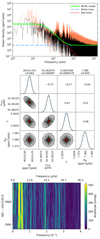Fig. A.10.

Summary figure for the B star HD 48977, which has a similar layout as shown in Fig. 3.

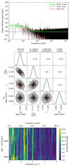Fig. A.11.

Summary figure for the B star HD 49677, which has a similar layout as shown in Fig. 3.

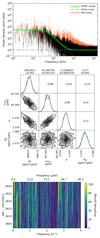Fig. A.12.

Summary figure for the A star HD 50747, which has a similar layout as shown in Fig. 3.

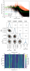Fig. A.13.

Summary figure for the A star HD 50844, which has a similar layout as shown in Fig. 3.

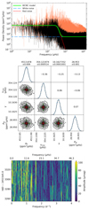Fig. A.14.

Summary figure for the A star HD 50870, which has a similar layout as shown in Fig. 3.

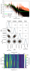Fig. A.15.

Summary figure for the B star HD 51193, which has a similar layout as shown in Fig. 3.

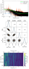Fig. A.16.

Summary figure for the F star HD 51332, which has a similar layout as shown in Fig. 3.

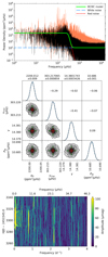Fig. A.17.

Summary figure for the F star HD 51359, which has a similar layout as shown in Fig. 3.

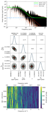Fig. A.18.

Summary figure for the B star HD 51452, which has a similar layout as shown in Fig. 3.

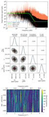Fig. A.19.

Summary figure for the A star HD 51722, which has a similar layout as shown in Fig. 3.

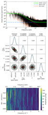Fig. A.20.

Summary figure for the B star HD 51756, which has a similar layout as shown in Fig. 3.

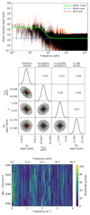Fig. A.21.

Summary figure for the A star HD 52130, which has a similar layout as shown in Fig. 3.

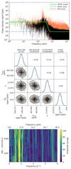Fig. A.22.

Summary figure for the A star HD 174532, which has a similar layout as shown in Fig. 3.

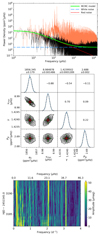Fig. A.23.

Summary figure for the F star HD 174589, which has a similar layout as shown in Fig. 3.

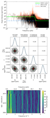Fig. A.24.

Summary figure for the A star HD 174936, which has a similar layout as shown in Fig. 3.

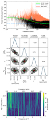Fig. A.25.

Summary figure for the A star HD 174966, which has a similar layout as shown in Fig. 3.

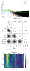Fig. A.26.

Summary figure for the B star HD 174967, which has a similar layout as shown in Fig. 3.

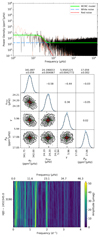Fig. A.27.

Summary figure for the A star HD 174990, which has a similar layout as shown in Fig. 3.

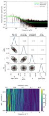Fig. A.28.

Summary figure for the F star HD 175272, which has a similar layout as shown in Fig. 3.

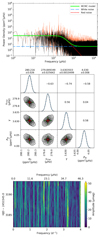Fig. A.29.

Summary figure for the A star HD 175445, which has a similar layout as shown in Fig. 3.

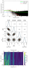Fig. A.30.

Summary figure for the A star HD 175542, which has a similar layout as shown in Fig. 3.

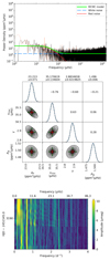Fig. A.31.

Summary figure for the B star HD 175640, which has a similar layout as shown in Fig. 3.

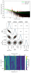Fig. A.32.

Summary figure for the A star HD 263425, which has a similar layout as shown in Fig. 3.

All Tables

Table 1.

Properties of the stars included in this work.

In the text

Table 2.

Optimised parameters for the extracted red noise (cf. Eq. (1)) for the stars studied in this paper using our Bayesian MCMC method, and the dominant cause(s) that are likely contributing to the observed low-frequency power excess, which are not only sourced from this work but also from the literature.

In the text

Table 3.

Expected TESS pulsation amplitudes for high-mass stars expressed as a relative percentage compared to the CoRoT and Kepler passbands.

In the text

All Figures

Fig. 1.

Tangential (top panel) and vertical (bottom panel) velocity spectra predicted by the 2D IGW simulations from Rogers et al. (2013), for three scenarios for the radial rotation profile: no rotation; rigid rotation with a rotation frequency of 1.1 d⁻¹ (12.7 μHz); and non-rigid rotation (Ω_core/Ω_env = 1.5) with a surface rotational frequency of 0.275 d⁻¹ (8.7 μHz), which are shown in green, blue and red, respectively. We note that the amplitudes of these spectra have been normalised to the dominant peak in each spectrum and have arbitrary units. The vertical grey lines show the theoretical pulsation mode frequencies for (ℓ,m) = (1, 0) in a 3 M_⊙ ZAMS star for radial orders in the range n ∈ [−25, −1] calculated by GYRE (Townsend & Teitler 2013) and each rotation scenario.

In the text

	Fig. 2. Spectral window function of the CoRoT data for HD 46150 up to 50 d⁻¹ (578.7 μHz) on a linear scale (top panel) and on a logarithmic scale (bottom panel).
In the text

Fig. 3.

Top panel: logarithmic power density spectrum of the CoRoT photometry for the O star HD 46150 is shown in black, and the best-fit model obtained using Eq. (1) is shown as the solid green line, with its red and white components shown as red short-dashed and blue long-dashed lines, respectively. Middle panel: posterior distributions from the Bayesian MCMC, with best-fit parameters obtained from Gaussian fits (shown in black) to the 1D histograms (shown in blue). Bottom panel: a sliding Fourier transform in the (linear) frequency range of 0 ≤ ν ≤ 4 d⁻¹ using a 15-d bin and a step of 0.1 d.

In the text

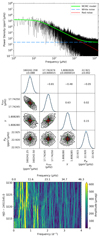	Fig. 4. Summary figure for the O star HD 46223, which has a similar layout as shown in Fig. 3.
In the text

	Fig. 5. Summary figure for the O star HD 46966, which has a similar layout as shown in Fig. 3, except that the original and residual power density spectra are shown in orange and black, respectively, since HD 49666 underwent pre-whitening of peaks with amplitude S/N ≥ 4.
In the text

Fig. 6.

Top row: pair-wise relationship between the fitting parameters, α₀, ν_char and γ in Eq. (1) shown for stars in our sample with spectroscopic parameters and sufficient CoRoT data for an accurate background fit. Bottom row: location of stars in the (spectroscopic) HR diagram as filled circles that have been colour-coded by the red-noise fit (Eq. (1)) parameters ν_char (left) and γ (right), with the size of each symbol corresponding to the fit parameter α₀. The location of stars with insufficient CoRoT data for an accurate background fit to the residual power density spectrum are shown as white triangles. Evolutionary tracks for representative masses (in units of M_⊙) from Ekström et al. (2012) are shown as solid grey lines, with the dashed grey line representing the ZAMS.

In the text

	Fig. 7. Measured profiles of red noise determined from the power density spectra of CoRoT photometry for stars with known stellar parameters from spectroscopy and sufficient CoRoT data for an accurate background fit to the residual power density spectrum, which have been colour-coded by their spectroscopic luminosity.
In the text

Fig. 8.

Distribution of measured characteristic frequencies, ν_char, as a function of stellar parameters given in solar units. The grey line represents the granulation frequency scaled using Eq. (3) with the Sun’s location indicated by the ⊙ symbol. The circles have been colour-coded by a star’s spectroscopic luminosity and the size of the symbol is proportional to the fitting parameter, α₀. White triangles represent stars which may have insufficient CoRoT data for an accurate determination for the fitting parameter γ (cf. Eq. (3)).

In the text

	Fig. 9. Histogram of fitting parameter γ (cf. Eq. (1)) for all stars with spectroscopic parameters and sufficient CoRoT data for an accurate background fit to the residual power density spectrum.
In the text

	Fig. 10. Location of the O and B stars that TESS is observing for 1 yr in its southern continuous viewing zone, with the colour-scale indicating the spectral type and the size of the symbol indicating the V-band magnitude.
In the text

	Fig. 11. Normalised Planck blackbody function for a T_eff = 10 000 K star, and hotter and cooler perturbations caused by pulsations are shown as black, blue and red solid lines, respectively. The approximate wavelength ranges for TESS, CoRoT and Kepler passbands are shown as dashed, dash-dot and dotted lines, respectively.
In the text

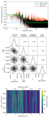	Fig. A.1. Summary figure for the B star HD 45418, which has a similar layout as shown in Fig. 3.
In the text

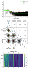	Fig. A.2. Summary figure for the A star HD 45517, which has a similar layout as shown in Fig. 3.
In the text

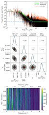	Fig. A.3. Summary figure for the B star HD 45546, which has a similar layout as shown in Fig. 3.
In the text

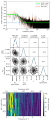	Fig. A.4. Summary figure for the O star HD 46149, which has a similar layout as shown in Fig. 3.
In the text

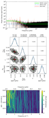	Fig. A.5. Summary figure for the B star HD 46179, which has a similar layout as shown in Fig. 3.
In the text

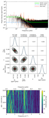	Fig. A.6. Summary figure for the O star HD 46202, which has a similar layout as shown in Fig. 3.
In the text

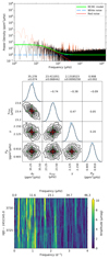	Fig. A.7. Summary figure for the B star HD 46769, which has a similar layout as shown in Fig. 3.
In the text

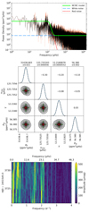	Fig. A.8. Summary figure for the A star HD 47485, which has a similar layout as shown in Fig. 3.
In the text

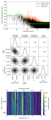	Fig. A.9. Summary figure for the F star HD 48784, which has a similar layout as shown in Fig. 3.
In the text

	Fig. A.10. Summary figure for the B star HD 48977, which has a similar layout as shown in Fig. 3.
In the text

	Fig. A.11. Summary figure for the B star HD 49677, which has a similar layout as shown in Fig. 3.
In the text

	Fig. A.12. Summary figure for the A star HD 50747, which has a similar layout as shown in Fig. 3.
In the text

	Fig. A.13. Summary figure for the A star HD 50844, which has a similar layout as shown in Fig. 3.
In the text

	Fig. A.14. Summary figure for the A star HD 50870, which has a similar layout as shown in Fig. 3.
In the text

	Fig. A.15. Summary figure for the B star HD 51193, which has a similar layout as shown in Fig. 3.
In the text

	Fig. A.16. Summary figure for the F star HD 51332, which has a similar layout as shown in Fig. 3.
In the text

	Fig. A.17. Summary figure for the F star HD 51359, which has a similar layout as shown in Fig. 3.
In the text

	Fig. A.18. Summary figure for the B star HD 51452, which has a similar layout as shown in Fig. 3.
In the text

	Fig. A.19. Summary figure for the A star HD 51722, which has a similar layout as shown in Fig. 3.
In the text

	Fig. A.20. Summary figure for the B star HD 51756, which has a similar layout as shown in Fig. 3.
In the text

	Fig. A.21. Summary figure for the A star HD 52130, which has a similar layout as shown in Fig. 3.
In the text

	Fig. A.22. Summary figure for the A star HD 174532, which has a similar layout as shown in Fig. 3.
In the text

	Fig. A.23. Summary figure for the F star HD 174589, which has a similar layout as shown in Fig. 3.
In the text

	Fig. A.24. Summary figure for the A star HD 174936, which has a similar layout as shown in Fig. 3.
In the text

	Fig. A.25. Summary figure for the A star HD 174966, which has a similar layout as shown in Fig. 3.
In the text

	Fig. A.26. Summary figure for the B star HD 174967, which has a similar layout as shown in Fig. 3.
In the text

	Fig. A.27. Summary figure for the A star HD 174990, which has a similar layout as shown in Fig. 3.
In the text

	Fig. A.28. Summary figure for the F star HD 175272, which has a similar layout as shown in Fig. 3.
In the text

	Fig. A.29. Summary figure for the A star HD 175445, which has a similar layout as shown in Fig. 3.
In the text

	Fig. A.30. Summary figure for the A star HD 175542, which has a similar layout as shown in Fig. 3.
In the text

	Fig. A.31. Summary figure for the B star HD 175640, which has a similar layout as shown in Fig. 3.
In the text

	Fig. A.32. Summary figure for the A star HD 263425, which has a similar layout as shown in Fig. 3.
In the text

Current usage metrics show cumulative count of Article Views (full-text article views including HTML views, PDF and ePub downloads, according to the available data) and Abstracts Views on Vision4Press platform.

Data correspond to usage on the plateform after 2015. The current usage metrics is available 48-96 hours after online publication and is updated daily on week days.

Initial download of the metrics may take a while.

[1] Abt, H. A., & Biggs, E. S. 1972, Bibliography of Stellar Radial Velocities (New York: Latham Process Corp) [Google Scholar]

[2] Abt, H. A., & Cardona, O. 1984, ApJ, 285, 190 [NASA ADS] [CrossRef] [Google Scholar]

[3] Abt, H. A., Levato, H., & Grosso, M. 2002, ApJ, 573, 359 [NASA ADS] [CrossRef] [Google Scholar]

[4] Adelman, S. J. 2001, A&A, 367, 297 [NASA ADS] [CrossRef] [EDP Sciences] [Google Scholar]

[5] Aerts, C., & Rogers, T. M. 2015, ApJ, 806, L33 [NASA ADS] [CrossRef] [Google Scholar]

[6] Aerts, C., Puls, J., Godart, M., & Dupret, M.-A. 2009, A&A, 508, 409 [NASA ADS] [CrossRef] [EDP Sciences] [Google Scholar]

[7] Aerts, C., Christensen-Dalsgaard, J., & Kurtz, D. W. 2010, Asteroseismology (Springer) [Google Scholar]

[8] Aerts, C., Briquet, M., Degroote, P., Thoul, A., & van Hoolst, T. 2011, A&A, 534, A98 [NASA ADS] [CrossRef] [EDP Sciences] [Google Scholar]

[9] Aerts, C., Simón-Díaz, S., Catala, C., et al. 2013, A&A, 557, A114 [NASA ADS] [CrossRef] [EDP Sciences] [Google Scholar]

[10] Aerts, C., Simón-Díaz, S., Groot, P. J., & Degroote, P. 2014, A&A, 569, A118 [NASA ADS] [CrossRef] [EDP Sciences] [Google Scholar]

[11] Aerts, C., Símon-Díaz, S., Bloemen, S., et al. 2017a, A&A, 602, A32 [NASA ADS] [CrossRef] [EDP Sciences] [Google Scholar]

[12] Aerts, C., Van Reeth, T., & Tkachenko, A. 2017b, ApJ, 847, L7 [NASA ADS] [CrossRef] [Google Scholar]

[13] Aerts, C., Bowman, D. M., Símon-Díaz, S., et al. 2018a, MNRAS, 476, 1234 [NASA ADS] [CrossRef] [Google Scholar]

[14] Aerts, C., Mathis, S., & Rogers, T. 2018b, ARA&A, submitted [arXiv:1809.07779] [Google Scholar]

[15] Ahmed, A., & Sigut, T. A. A. 2017, MNRAS, 471, 3398 [NASA ADS] [CrossRef] [Google Scholar]

[16] Aldoretta, E. J., Caballero-Nieves, S. M., Gies, D. R., et al. 2015, AJ, 149, 26 [NASA ADS] [CrossRef] [Google Scholar]

[17] Appourchaux, T. 2003, Ap&SS, 284, 109 [NASA ADS] [CrossRef] [Google Scholar]

[18] Appourchaux, T. 2008, Astron. Nachr., 329, 485 [NASA ADS] [CrossRef] [Google Scholar]

[19] Appourchaux, T., Gizon, L., & Rabello-Soares, M.-C. 1998, A&AS, 132, 107 [NASA ADS] [CrossRef] [EDP Sciences] [Google Scholar]

[20] Appourchaux, T., Michel, E., Auvergne, M., et al. 2008, A&A, 488, 705 [NASA ADS] [CrossRef] [EDP Sciences] [Google Scholar]

[21] Augustson, K. C., Brun, A. S., & Toomre, J. 2016, ApJ, 829, 92 [NASA ADS] [CrossRef] [Google Scholar]

[22] Auvergne, M., Bodin, P., Boisnard, L., et al. 2009, A&A, 506, 411 [NASA ADS] [CrossRef] [EDP Sciences] [Google Scholar]

[23] Bailer-Jones, C. A. L. 2011, MNRAS, 411, 435 [NASA ADS] [CrossRef] [Google Scholar]

[24] Balona, L. A. 1992, MNRAS, 254, 403 [NASA ADS] [CrossRef] [Google Scholar]

[25] Balona, L. A. 2014, MNRAS, 439, 3453 [NASA ADS] [CrossRef] [Google Scholar]

[26] Barceló Forteza, S., Roca Cortés, T., García Hernández, A., & García, R. A. 2017, A&A, 601, A57 [NASA ADS] [CrossRef] [EDP Sciences] [Google Scholar]

[27] Baumgardt, H., Dettbarn, C., & Wielen, R. 2000, A&AS, 146, 251 [NASA ADS] [CrossRef] [EDP Sciences] [Google Scholar]

[28] Belkacem, K., Dupret, M. A., & Noels, A. 2010, A&A, 510, A6 [NASA ADS] [CrossRef] [EDP Sciences] [Google Scholar]

[29] Benomar, O., Appourchaux, T., & Baudin, F. 2009, A&A, 506, 15 [NASA ADS] [CrossRef] [EDP Sciences] [Google Scholar]

[30] Blomme, R., Mahy, L., Catala, C., et al. 2011, A&A, 533, A4 [NASA ADS] [CrossRef] [EDP Sciences] [Google Scholar]

[31] Bonatto, C., & Bica, E. 2009, MNRAS, 394, 2127 [NASA ADS] [CrossRef] [Google Scholar]

[32] Borucki, W. J., Koch, D., Basri, G., et al. 2010, Science, 327, 977 [NASA ADS] [CrossRef] [PubMed] [Google Scholar]

[33] Bowman, D. M. 2016, PhD Thesis Jeremiah Horrocks Institute, University of Central Lancashire, Preston, UK [Google Scholar]

[34] Bowman, D. M. 2017, Amplitude Modulation of Pulsation Modes in Delta Scuti Stars (Springer International Publishing) [CrossRef] [Google Scholar]

[35] Bowman, D. M., & Kurtz, D. W. 2018, MNRAS, 476, 3169 [NASA ADS] [CrossRef] [Google Scholar]

[36] Bowman, D. M., Holdsworth, D. L., & Kurtz, D. W. 2015, MNRAS, 449, 1004 [NASA ADS] [CrossRef] [Google Scholar]

[37] Bowman, D. M., Kurtz, D. W., Breger, M., Murphy, S. J., & Holdsworth, D. L. 2016, MNRAS, 460, 1970 [NASA ADS] [CrossRef] [Google Scholar]

[38] Bragança, G. A., Daflon, S., Cunha, K., et al. 2012, AJ, 144, 130 [NASA ADS] [CrossRef] [Google Scholar]

[39] Breger, M. 2000, MNRAS, 313, 129 [CrossRef] [Google Scholar]

[40] Breger, M., Stich, J., Garrido, R., et al. 1993, A&A, 271, 482 [NASA ADS] [Google Scholar]

[41] Breger, M., Pamyatnykh, A. A., Zima, W., et al. 2002, MNRAS, 336, 249 [NASA ADS] [CrossRef] [Google Scholar]

[42] Breger, M., Rodler, F., Pretorius, M. L., et al. 2004, A&A, 419, 695 [NASA ADS] [CrossRef] [EDP Sciences] [Google Scholar]

[43] Briquet, M., Aerts, C., Baglin, A., et al. 2011, A&A, 527, A112 [NASA ADS] [CrossRef] [EDP Sciences] [Google Scholar]

[44] Browning, M. K., Brun, A. S., & Toomre, J. 2004, ApJ, 601, 512 [NASA ADS] [CrossRef] [Google Scholar]

[45] Buysschaert, B., Aerts, C., Bloemen, S., et al. 2015, MNRAS, 453, 89 [NASA ADS] [CrossRef] [Google Scholar]

[46] Buysschaert, B., Neiner, C., Richardson, N. D., et al. 2017, A&A, 602, A91 [NASA ADS] [CrossRef] [EDP Sciences] [Google Scholar]

[47] Buysschaert, B., Aerts, C., Bowman, D. M., et al. 2018, A&A, 616, A148 [NASA ADS] [CrossRef] [EDP Sciences] [Google Scholar]

[48] Cantiello, M., Langer, N., Brott, I., et al. 2009a, A&A, 499, 279 [NASA ADS] [CrossRef] [EDP Sciences] [Google Scholar]

[49] Cantiello, M., Langer, N., Brott, I., et al. 2009b, Commun. Asteroseismol., 158, 61 [NASA ADS] [Google Scholar]

[50] Cantiello, M., Mankovich, C., Bildsten, L., Christensen-Dalsgaard, J., & Paxton, B. 2014, ApJ, 788, 93 [NASA ADS] [CrossRef] [Google Scholar]

[51] Casagrande, L., Schönrich, R., Asplund, M., et al. 2011, A&A, 530, A138 [NASA ADS] [CrossRef] [EDP Sciences] [Google Scholar]

[52] Castelli, F., & Hubrig, S. 2004, A&A, 425, 263 [NASA ADS] [CrossRef] [EDP Sciences] [Google Scholar]

[53] Chaplin, W. J., & Miglio, A. 2013, ARA&A, 51, 353 [NASA ADS] [CrossRef] [Google Scholar]

[54] Charbonnel, C., & Talon, S. 2005, Science, 309, 2189 [NASA ADS] [CrossRef] [PubMed] [Google Scholar]

[55] Charbonnel, C., Decressin, T., Amard, L., Palacios, A., & Talon, S. 2013, A&A, 554, A40 [NASA ADS] [CrossRef] [EDP Sciences] [Google Scholar]

[56] Chini, R., Hoffmeister, V. H., Nasseri, A., Stahl, O., & Zinnecker, H. 2012, MNRAS, 424, 1925 [NASA ADS] [CrossRef] [Google Scholar]

[57] Claria, J. J. 1972, A&A, 19, 303 [NASA ADS] [Google Scholar]

[58] Couston, L.-A., Lecoanet, D., Favier, B., & Le Bars, M. 2018, J. Fluid Mech., 854, R3 [CrossRef] [Google Scholar]

[59] David, T. J., & Hillenbrand, L. A. 2015, ApJ, 804, 146 [NASA ADS] [CrossRef] [Google Scholar]

[60] Davies, G. R., Silva Aguirre, V., Bedding, T. R., et al. 2016, MNRAS, 456, 2183 [NASA ADS] [CrossRef] [Google Scholar]

[61] de Bruijne, J. H. J., & Eilers, A.-C. 2012, A&A, 546, A61 [NASA ADS] [CrossRef] [EDP Sciences] [Google Scholar]

[62] Degroote, P., Briquet, M., Catala, C., et al. 2009, A&A, 506, 111 [NASA ADS] [CrossRef] [EDP Sciences] [Google Scholar]

[63] Degroote, P., Aerts, C., Baglin, A., et al. 2010a, Nature, 464, 259 [NASA ADS] [CrossRef] [PubMed] [Google Scholar]

[64] Degroote, P., Aerts, C., Samadi, R., et al. 2010b, Astron. Nachr., 331, 1065 [NASA ADS] [CrossRef] [Google Scholar]

[65] Degroote, P., Briquet, M., Auvergne, M., et al. 2010c, A&A, 519, A38 [NASA ADS] [CrossRef] [EDP Sciences] [Google Scholar]

[66] Degroote, P., Acke, B., Samadi, R., et al. 2011, A&A, 536, A82 [NASA ADS] [CrossRef] [EDP Sciences] [Google Scholar]

[67] Dolez, N., Vauclair, S., Michel, E., et al. 2009, A&A, 506, 159 [NASA ADS] [CrossRef] [EDP Sciences] [Google Scholar]

[68] Dolk, L., Wahlgren, G. M., Lundberg, H., et al. 2002, A&A, 385, 111 [NASA ADS] [CrossRef] [EDP Sciences] [Google Scholar]

[69] Dommanget, J., & Nys, O. 2000, A&A, 363, 991 [NASA ADS] [Google Scholar]

[70] Douglass, G. G., Mason, B. D., Germain, M. E., & Worley, C. E. 1999, AJ, 118, 1395 [NASA ADS] [CrossRef] [Google Scholar]

[71] Dziembowski, W. A., & Pamyatnykh, A. A. 2008, MNRAS, 385, 2061 [NASA ADS] [CrossRef] [Google Scholar]

[72] Edelmann, P. V. F., Ratnasingam, R. P., Pedersen, M. G., et al. 2018, ApJ, submitted [Google Scholar]

[73] Eggenberger, P., Lagarde, N., Miglio, A., et al. 2017, A&A, 599, A18 [NASA ADS] [CrossRef] [EDP Sciences] [Google Scholar]

[74] Eggleton, P. P., & Tokovinin, A. A. 2008, MNRAS, 389, 869 [NASA ADS] [CrossRef] [Google Scholar]

[75] Ekström, S., Georgy, C., Eggenberger, P., et al. 2012, A&A, 537, A146 [NASA ADS] [CrossRef] [EDP Sciences] [Google Scholar]

[76] Fabricius, C., Høg, E., Makarov, V. V., et al. 2002, A&A, 384, 180 [NASA ADS] [CrossRef] [EDP Sciences] [Google Scholar]

[77] Foreman-Mackey, D., Hogg, D. W., Lang, D., & Goodman, J. 2013, PASP, 125, 306 [CrossRef] [Google Scholar]

[78] Fossati, L., Castro, N., Schöller, M., et al. 2015, A&A, 582, A45 [NASA ADS] [CrossRef] [EDP Sciences] [Google Scholar]

[79] Fox Machado, L., Michel, R., Álvarez, M., et al. 2008, Commun. Asteroseismol., 153, 20 [NASA ADS] [CrossRef] [Google Scholar]

[80] Fox Machado, L., Alvarez, M., Michel, R., et al. 2010, New Astron., 15, 397 [NASA ADS] [CrossRef] [Google Scholar]

[81] Frankowski, A., Jancart, S., & Jorissen, A. 2007, A&A, 464, 377 [NASA ADS] [CrossRef] [EDP Sciences] [Google Scholar]

[82] Frémat, Y., Neiner, C., Hubert, A.-M., et al. 2006, A&A, 451, 1053 [NASA ADS] [CrossRef] [EDP Sciences] [Google Scholar]

[83] Fuller, J., Lecoanet, D., Cantiello, M., & Brown, B. 2014, ApJ, 796, 17 [Google Scholar]

[84] Fuller, J., Cantiello, M., Lecoanet, D., & Quataert, E. 2015, ApJ, 810, 101 [NASA ADS] [CrossRef] [Google Scholar]

[85] Fullerton, A. W. 1990, PhD Thesis, Toronto Univ. (Ontario, Canada) [Google Scholar]

[86] Fullerton, A. W., Gies, D. R., & Bolton, C. T. 1996, ApJS, 103, 475 [NASA ADS] [CrossRef] [Google Scholar]

[87] Fullerton, A. W., Massa, D. L., & Prinja, R. K. 2006, ApJ, 637, 1025 [NASA ADS] [CrossRef] [Google Scholar]

[88] García Hernández, A., Moya, A., Michel, E., et al. 2009, A&A, 506, 79 [NASA ADS] [CrossRef] [EDP Sciences] [Google Scholar]

[89] García Hernández, A., Moya, A., Michel, E., et al. 2013, A&A, 559, A63 [NASA ADS] [CrossRef] [EDP Sciences] [Google Scholar]

[90] Gaulme, P., Appourchaux, T., & Boumier, P. 2009, A&A, 506, 7 [NASA ADS] [CrossRef] [EDP Sciences] [Google Scholar]

[91] Gebran, M., Farah, W., Paletou, F., Monier, R., & Watson, V. 2016, A&A, 589, A83 [NASA ADS] [CrossRef] [EDP Sciences] [Google Scholar]

[92] Gelman, A., & Rubin, D. B. 1992, Stat. Sci., 7, 457 [Google Scholar]

[93] Germain, M. E., Douglass, G. G., & Worley, C. E. 1999, AJ, 117, 2511 [NASA ADS] [CrossRef] [Google Scholar]

[94] Ghazaryan, S., Alecian, G., & Harutyunian, H. 2013, MNRAS, 435, 1852 [NASA ADS] [CrossRef] [Google Scholar]

[95] Godart, M., Simón-Díaz, S., Herrero, A., et al. 2017, A&A, 597, A23 [NASA ADS] [CrossRef] [EDP Sciences] [Google Scholar]

[96] Gontcharov, G. A. 2006, Astron. Lett., 32, 759 [NASA ADS] [CrossRef] [Google Scholar]

[97] Grassitelli, L., Fossati, L., Simón-Diáz, S., et al. 2015, ApJ, 808, L31 [NASA ADS] [CrossRef] [Google Scholar]

[98] Gruberbauer, M., Kallinger, T., Weiss, W. W., & Guenther, D. B. 2009, A&A, 506, 1043 [NASA ADS] [CrossRef] [EDP Sciences] [Google Scholar]

[99] Grunhut, J. H., Wade, G. A., Neiner, C., et al. 2017, MNRAS, 465, 2432 [NASA ADS] [CrossRef] [Google Scholar]

[100] Gutiérrez-Soto, J., Fabregat, J., Suso, J., et al. 2007, A&A, 476, 927 [NASA ADS] [CrossRef] [EDP Sciences] [Google Scholar]

[101] Gutiérrez-Soto, J., Neiner, C., Fabregat, J., et al. 2011, in Active OB Stars: Structure, Evolution, Mass Loss, and Critical Limits, eds. C. Neiner, G. Wade, G. Meynet, & G. Peters, IAU Symp., 272, 451 [NASA ADS] [Google Scholar]

[102] Hambleton, K. M. 2016, PhD Thesis, Jeremiah Horrocks Institute, University of Central Lancashire, UK [Google Scholar]

[103] Hambleton, K., Fuller, J., Thompson, S., et al. 2018, MNRAS, 473, 5165 [NASA ADS] [CrossRef] [Google Scholar]

[104] Handberg, R., & Campante, T. L. 2011, A&A, 527, A56 [NASA ADS] [CrossRef] [EDP Sciences] [Google Scholar]

[105] Handler, G., Matthews, J. M., Eaton, J. A., et al. 2009, ApJ, 698, L56 [NASA ADS] [CrossRef] [Google Scholar]

[106] Harvey, J. 1985, in Future Missions in Solar, Heliospheric & Space Plasma Physics, eds. E. Rolfe, & B. Battrick, ESA SP, 235 [Google Scholar]

[107] Hauck, B., & Mermilliod, M. 1998, A&AS, 129, 431 [NASA ADS] [CrossRef] [EDP Sciences] [Google Scholar]

[108] Heger, A., Langer, N., & Woosley, S. E. 2000, ApJ, 528, 368 [NASA ADS] [CrossRef] [Google Scholar]

[109] Hekker, S., & Ball, W. H. 2014, A&A, 564, A105 [NASA ADS] [CrossRef] [EDP Sciences] [Google Scholar]

[110] Hekker, S., & Christensen-Dalsgaard, J. 2017, A&ARv, 25, 1 [NASA ADS] [CrossRef] [EDP Sciences] [Google Scholar]

[111] Hensberge, H., Pavlovski, K., & Verschueren, W. 2000, A&A, 358, 553 [NASA ADS] [Google Scholar]

[112] Hohle, M. M., Neuhäuser, R., & Schutz, B. F. 2010, Astron. Nachr., 331, 349 [NASA ADS] [CrossRef] [Google Scholar]

[113] Holmberg, J., Nordström, B., & Andersen, J. 2009, A&A, 501, 941 [NASA ADS] [CrossRef] [EDP Sciences] [Google Scholar]

[114] Houk, N., & Swift, C. 1999, Michigan Catalogue of Two-dimensional Spectral Types for the HD Stars (University of Michigan), 5 [Google Scholar]

[115] Howarth, I. D., Goss, K. J. F., Stevens, I. R., Chaplin, W. J., & Elsworth, Y. 2014, MNRAS, 440, 1674 [NASA ADS] [CrossRef] [Google Scholar]

[116] Howell, S. B., Sobeck, C., Haas, M., et al. 2014, PASP, 126, 398 [NASA ADS] [CrossRef] [Google Scholar]

[117] Huber, D., Stello, D., Bedding, T. R., et al. 2009, Commun. Asteroseismol., 160, 74 [NASA ADS] [CrossRef] [Google Scholar]

[118] Hubrig, S., Castelli, F., Mathys, G., & Wahlgren, G. M. 2001, in Magnetic Fields Across the Hertzsprung-Russell Diagram, eds. G. Mathys, S. K. Solanki, & D. T. Wickramasinghe, ASP Conf. Ser., 248, 387 [NASA ADS] [Google Scholar]

[119] Iijima, T., & Ishida, K. 1978, PASJ, 30, 657 [NASA ADS] [Google Scholar]

[120] Johnston, C., Buysschaert, B., Tkachenko, A., Aerts, C., & Neiner, C. 2017, MNRAS, 469, L118 [NASA ADS] [CrossRef] [Google Scholar]

[121] Kallinger, T., & Matthews, J. M. 2010, ApJ, 711, L35 [NASA ADS] [CrossRef] [Google Scholar]

[122] Kallinger, T., De Ridder, J., Hekker, S., et al. 2014, A&A, 570, A41 [NASA ADS] [CrossRef] [EDP Sciences] [Google Scholar]

[123] Kjeldsen, H., & Bedding, T. R. 1995, A&A, 293, 87 [NASA ADS] [Google Scholar]

[124] Kochukhov, O., Johnston, C., Alecian, E., & Wade, G. A. 2018, MNRAS, 478, 1749 [NASA ADS] [CrossRef] [Google Scholar]

[125] Koen, C., & Eyer, L. 2002, MNRAS, 331, 45 [NASA ADS] [CrossRef] [Google Scholar]

[126] Krtička, J., & Feldmeier, A. 2018, A&A, 617, A121 [NASA ADS] [CrossRef] [EDP Sciences] [Google Scholar]

[127] Kurtz, D. W., Cameron, C., Cunha, M. S., et al. 2005, MNRAS, 358, 651 [NASA ADS] [CrossRef] [Google Scholar]

[128] Kurtz, D. W., Saio, H., Takata, M., et al. 2014, MNRAS, 444, 102 [NASA ADS] [CrossRef] [Google Scholar]

[129] Kurtz, D. W., Shibahashi, H., Murphy, S. J., Bedding, T. R., & Bowman, D. M. 2015, MNRAS, 450, 3015 [NASA ADS] [CrossRef] [Google Scholar]

[130] Landstreet, J. D., Kupka, F., Ford, H. A., et al. 2009, A&A, 503, 973 [NASA ADS] [CrossRef] [EDP Sciences] [Google Scholar]

[131] Lecoanet, D., & Quataert, E. 2013, MNRAS, 430, 2363 [NASA ADS] [CrossRef] [Google Scholar]

[132] Lecoanet, D., Vasil, G. M., Fuller, J., Cantiello, M., & Burns, K. J. 2017, MNRAS, 466, 2181 [NASA ADS] [CrossRef] [Google Scholar]

[133] Lee, U., Neiner, C., & Mathis, S. 2014, MNRAS, 443, 1515 [NASA ADS] [CrossRef] [Google Scholar]

[134] Lefever, K., Puls, J., & Aerts, C. 2007, A&A, 463, 1093 [NASA ADS] [CrossRef] [EDP Sciences] [Google Scholar]

[135] Lefever, K., Puls, J., Morel, T., et al. 2010, A&A, 515, A74 [NASA ADS] [CrossRef] [EDP Sciences] [Google Scholar]

[136] Lefèvre, L., Marchenko, S. V., Moffat, A. F. J., & Acker, A. 2009, A&A, 507, 1141 [NASA ADS] [CrossRef] [EDP Sciences] [Google Scholar]

[137] Levato, H., & Malaroda, S. 1974, AJ, 79, 890 [NASA ADS] [CrossRef] [Google Scholar]

[138] Liu, T., Janes, K. A., & Bania, T. M. 1989, AJ, 98, 626 [NASA ADS] [CrossRef] [Google Scholar]

[139] Liu, C.-Y., Doressoundiram, A., Roques, F., et al. 2015, MNRAS, 446, 932 [NASA ADS] [CrossRef] [Google Scholar]

[140] Lyubimkov, L. S., Lambert, D. L., Rachkovskaya, T. M., et al. 2000, MNRAS, 316, 19 [NASA ADS] [CrossRef] [Google Scholar]

[141] Lyubimkov, L. S., Rachkovskaya, T. M., Rostopchin, S. I., & Lambert, D. L. 2002, MNRAS, 333, 9 [NASA ADS] [CrossRef] [Google Scholar]

[142] Lyubimkov, L. S., Rostopchin, S. I., Rachkovskaya, T. M., Poklad, D. B., & Lambert, D. L. 2005, MNRAS, 358, 193 [NASA ADS] [CrossRef] [Google Scholar]

[143] Lyubimkov, L. S., Lambert, D. L., Poklad, D. B., Rachkovskaya, T. M., & Rostopchin, S. I. 2013, MNRAS, 428, 3497 [NASA ADS] [Google Scholar]

[144] Maeder, A. 2009, Physics, Formation and Evolution of Rotating Stars (Springer) [Google Scholar]

[145] Maeder, A., & Meynet, G. 2000, ARA&A, 38, 143 [NASA ADS] [CrossRef] [Google Scholar]

[146] Mahy, L., Nazé, Y., Rauw, G., et al. 2009, A&A, 502, 937 [NASA ADS] [CrossRef] [EDP Sciences] [Google Scholar]

[147] Maíz Apellániz, J. 2010, A&A, 518, A1 [NASA ADS] [CrossRef] [EDP Sciences] [Google Scholar]

[148] Maíz-Apellániz, J., Walborn, N. R., Galué, H. Á., & Wei, L. H. 2004, ApJS, 151, 103 [NASA ADS] [CrossRef] [Google Scholar]

[149] Makaganiuk, V., Kochukhov, O., Piskunov, N., et al. 2011, A&A, 525, A97 [NASA ADS] [CrossRef] [EDP Sciences] [Google Scholar]

[150] Mantegazza, L., Poretti, E., Michel, E., et al. 2012, A&A, 542, A24 [NASA ADS] [CrossRef] [EDP Sciences] [Google Scholar]

[151] Martins, F., Schaerer, D., Hillier, D. J., et al. 2005, A&A, 441, 735 [NASA ADS] [CrossRef] [EDP Sciences] [Google Scholar]

[152] Martins, F., Mahy, L., Hillier, D. J., & Rauw, G. 2012, A&A, 538, A39 [NASA ADS] [CrossRef] [EDP Sciences] [Google Scholar]

[153] Martins, F., Hervé, A., Bouret, J.-C., et al. 2015, A&A, 575, A34 [NASA ADS] [CrossRef] [EDP Sciences] [Google Scholar]

[154] Masana, E., Jordi, C., & Ribas, I. 2006, A&A, 450, 735 [NASA ADS] [CrossRef] [EDP Sciences] [Google Scholar]

[155] Mason, B. D., Gies, D. R., Hartkopf, W. I., et al. 1998, AJ, 115, 821 [NASA ADS] [CrossRef] [Google Scholar]

[156] Mason, B. D., Wycoff, G. L., Hartkopf, W. I., Douglass, G. G., & Worley, C. E. 2001, AJ, 122, 3466 [Google Scholar]

[157] Massey, P., Johnson, K. E., & Degioia-Eastwood, K. 1995, ApJ, 454, 151 [NASA ADS] [CrossRef] [Google Scholar]

[158] Mathis, S. 2009, A&A, 506, 811 [NASA ADS] [CrossRef] [EDP Sciences] [Google Scholar]

[159] Mathis, S., & de Brye, N. 2011, A&A, 526, A65 [NASA ADS] [CrossRef] [EDP Sciences] [Google Scholar]

[160] Mathis, S., Neiner, C., & Tran Minh, N. 2014, A&A, 565, A47 [NASA ADS] [CrossRef] [EDP Sciences] [Google Scholar]

[161] McCuskey, S. W. 1956, ApJS, 2, 271 [NASA ADS] [CrossRef] [Google Scholar]

[162] McDonald, I., Zijlstra, A. A., & Boyer, M. L. 2012, MNRAS, 427, 343 [NASA ADS] [CrossRef] [Google Scholar]

[163] Merrill, P. W., Humason, M. L., & Burwell, C. G. 1925, ApJ, 61, 389 [NASA ADS] [CrossRef] [Google Scholar]

[164] Meynet, G., Ekstrom, S., Maeder, A., et al. 2013, in Lect. Notes Phys., eds. M. Goupil, K. Belkacem, C. Neiner, et al. (Berlin: Springer Verlag), 865, 3 [NASA ADS] [CrossRef] [Google Scholar]

[165] Michel, E., Baglin, A., Auvergne, M., et al. 2006, in The CoRoT Mission Pre-Launch Status– Stellar Seismology and Planet Finding, eds. M. Fridlund, A. Baglin, J. Lochard, & L. Conroy, ESA SP, 1306, 39 [NASA ADS] [Google Scholar]

[166] Michel, E., Baglin, A., Auvergne, M., et al. 2008, Science, 322, 558 [NASA ADS] [CrossRef] [PubMed] [Google Scholar]

[167] Moffat, A. F. J., Marchenko, S. V., Zhilyaev, B. E., et al. 2008, ApJ, 679, L45 [NASA ADS] [CrossRef] [Google Scholar]

[168] Mokiem, M. R., de Koter, A., Vink, J. S., et al. 2007, A&A, 473, 603 [NASA ADS] [CrossRef] [EDP Sciences] [Google Scholar]

[169] Monnier, J. D., Townsend, R. H. D., Che, X., et al. 2010, ApJ, 725, 1192 [NASA ADS] [CrossRef] [Google Scholar]

[170] Montalban, J. 1994, A&A, 281, 421 [NASA ADS] [Google Scholar]

[171] Montalban, J., & Schatzman, E. 1996, A&A, 305, 513 [NASA ADS] [Google Scholar]

[172] Moravveji, E. 2016, MNRAS, 455, L67 [NASA ADS] [Google Scholar]

[173] Morel, T., Castro, N., Fossati, L., et al. 2014, The Messenger, 157, 27 [NASA ADS] [Google Scholar]

[174] Morel, T., Castro, N., Fossati, L., et al. 2015, in New Windows on Massive Stars, eds. G. Meynet, C. Georgy, J. Groh, & P. Stee, IAU Symp., 307, 342 [NASA ADS] [Google Scholar]

[175] Mowlavi, N., Barblan, F., Saesen, S., & Eyer, L. 2013, A&A, 554, A108 [NASA ADS] [CrossRef] [EDP Sciences] [Google Scholar]

[176] Mugnes, J.-M., & Robert, C. 2015, MNRAS, 454, 28 [NASA ADS] [Google Scholar]

[177] Munari, U., & Tomasella, L. 1999, A&AS, 137, 521 [NASA ADS] [CrossRef] [EDP Sciences] [Google Scholar]

[178] Murphy, S. J., & Paunzen, E. 2017, MNRAS, 466, 546 [NASA ADS] [CrossRef] [Google Scholar]

[179] Murphy, S. J., Fossati, L., Bedding, T. R., et al. 2016, MNRAS, 459, 1201 [NASA ADS] [CrossRef] [Google Scholar]

[180] Neiner, C., Floquet, M., Samadi, R., et al. 2012, A&A, 546, A47 [NASA ADS] [CrossRef] [EDP Sciences] [Google Scholar]

[181] Neiner, C., Mathis, S., Saio, H., & Lee, U. 2013, in Progress in Physics of the Sun and Stars: A New Era in Helio- and Asteroseismology, eds. H. Shibahashi, & A. E. Lynas-Gray, ASP Conf. Ser., 479, 319 [NASA ADS] [Google Scholar]

[182] Niemczura, E., Morel, T., & Aerts, C. 2009, A&A, 506, 213 [NASA ADS] [CrossRef] [EDP Sciences] [Google Scholar]

[183] Ouazzani, R.-M., Salmon, S. J. A. J., Antoci, V., et al. 2017, MNRAS, 465, 2294 [NASA ADS] [CrossRef] [Google Scholar]

[184] Ouazzani, R. M., Marques, J. P., Goupil, M., et al. 2018, A&A, submitted [arXiv:1801.09228] [Google Scholar]

[185] Owocki, S. P., & Rybicki, G. B. 1984, ApJ, 284, 337 [NASA ADS] [CrossRef] [Google Scholar]

[186] Ozel, N., Mosser, B., Dupret, M. A., et al. 2013, A&A, 558, A79 [CrossRef] [EDP Sciences] [Google Scholar]

[187] Pantillon, F. P., Talon, S., & Charbonnel, C. 2007, A&A, 474, 155 [NASA ADS] [CrossRef] [EDP Sciences] [Google Scholar]

[188] Pápics, P. I., Briquet, M., Auvergne, M., et al. 2011, A&A, 528, A123 [NASA ADS] [CrossRef] [EDP Sciences] [Google Scholar]

[189] Pápics, P. I., Briquet, M., Baglin, A., et al. 2012, A&A, 542, A55 [NASA ADS] [CrossRef] [EDP Sciences] [Google Scholar]

[190] Pápics, P. I., Moravveji, E., Aerts, C., et al. 2014, A&A, 570, A8 [NASA ADS] [CrossRef] [EDP Sciences] [Google Scholar]

[191] Pápics, P. I., Tkachenko, A., Van Reeth, T., et al. 2017, A&A, 598, A74 [NASA ADS] [CrossRef] [EDP Sciences] [Google Scholar]

[192] Pascual-Granado, J., Garrido, R., & Suárez, J. C. 2015, A&A, 581, A89 [NASA ADS] [EDP Sciences] [Google Scholar]

[193] Paunzen, E., Duffee, B., Heiter, U., Kuschnig, R., & Weiss, W. W. 2001, A&A, 373, 625 [NASA ADS] [CrossRef] [EDP Sciences] [Google Scholar]

[194] Paunzen, E., Iliev, I. K., Kamp, I., & Barzova, I. S. 2002, MNRAS, 336, 1030 [NASA ADS] [CrossRef] [Google Scholar]

[195] Paxton, B., Bildsten, L., Dotter, A., et al. 2011, ApJS, 192, 3 [Google Scholar]

[196] Paxton, B., Cantiello, M., Arras, P., et al. 2013, ApJS, 208, 4 [NASA ADS] [CrossRef] [Google Scholar]

[197] Paxton, B., Marchant, P., Schwab, J., et al. 2015, ApJS, 220, 15 [Google Scholar]

[198] Paxton, B., Schwab, J., Bauer, E. B., et al. 2018, ApJS, 234, 34 [NASA ADS] [CrossRef] [EDP Sciences] [Google Scholar]

[199] Pedersen, M. G., Aerts, C., Pápics, P. I., & Rogers, T. M. 2018, A&A, 614, A128 [NASA ADS] [CrossRef] [EDP Sciences] [Google Scholar]

[200] Plaskett, J. S., & Pearce, J. A. 1931, Publ. Dominion Astrophys. Obs. Vic., 5, 1 [NASA ADS] [Google Scholar]

[201] Plumb, R. A., & McEwan, A. D. 1978, J. Atm. Sci., 35, 1827 [NASA ADS] [CrossRef] [MathSciNet] [Google Scholar]

[202] Poretti, E., Garrido, R., Amado, P. J., et al. 2003, A&A, 406, 203 [NASA ADS] [CrossRef] [EDP Sciences] [Google Scholar]

[203] Poretti, E., Alonso, R., Amado, P. J., et al. 2005, AJ, 129, 2461 [NASA ADS] [CrossRef] [Google Scholar]

[204] Poretti, E., Michel, E., Garrido, R., et al. 2009, A&A, 506, 85 [NASA ADS] [CrossRef] [EDP Sciences] [Google Scholar]

[205] Press, W. H. 1981, ApJ, 245, 286 [NASA ADS] [CrossRef] [Google Scholar]

[206] Prugniel, P., & Soubiran, C. 2001, A&A, 369, 1048 [NASA ADS] [CrossRef] [EDP Sciences] [Google Scholar]

[207] Puls, J., Kudritzki, R.-P., Herrero, A., et al. 1996, A&A, 305, 171 [NASA ADS] [Google Scholar]

[208] Puls, J., Markova, N., Scuderi, S., et al. 2006, A&A, 454, 625 [NASA ADS] [CrossRef] [EDP Sciences] [Google Scholar]

[209] Puls, J., Vink, J. S., & Najarro, F. 2008, A&ARv, 16, 209 [NASA ADS] [CrossRef] [EDP Sciences] [Google Scholar]

[210] Ramiaramanantsoa, T., Moffat, A. F. J., Harmon, R., et al. 2018, MNRAS, 473, 5532 [NASA ADS] [CrossRef] [EDP Sciences] [Google Scholar]

[211] Rauw, G., De Becker, M., van Winckel, H., et al. 2008, A&A, 487, 659 [NASA ADS] [CrossRef] [EDP Sciences] [Google Scholar]

[212] Renson, P., & Manfroid, J. 2009, A&A, 498, 961 [NASA ADS] [CrossRef] [EDP Sciences] [Google Scholar]

[213] Ricker, G. R., Winn, J. N., Vanderspek, R., et al. 2015, J. Astron. Telescopes Instrum. Syst., 1, 014003 [Google Scholar]

[214] Rieutord, M., Triana, S. A., Zimmerman, D. S., & Lathrop, D. P. 2012, Phys. Rev. E, 86, 026304 [NASA ADS] [Google Scholar]

[215] Roberts, Jr., L. C., Tokovinin, A., Mason, B. D., Hartkopf, W. I., & Riddle, R. L. 2015, AJ, 150, 130 [NASA ADS] [Google Scholar]

[216] Rogers, T. M. 2015, ApJ, 815, L30 [NASA ADS] [CrossRef] [Google Scholar]

[217] Rogers, T. M., & MacGregor, K. B. 2010, MNRAS, 401, 191 [NASA ADS] [CrossRef] [Google Scholar]

[218] Rogers, T. M., & MacGregor, K. B. 2011, MNRAS, 410, 946 [NASA ADS] [CrossRef] [Google Scholar]

[219] Rogers, T. M., & McElwaine, J. N. 2017, ApJ, 848, L1 [NASA ADS] [CrossRef] [Google Scholar]

[220] Rogers, T. M., Lin, D. N. C., McElwaine, J. N., & Lau, H. H. B. 2013, ApJ, 772, 21 [NASA ADS] [CrossRef] [Google Scholar]

[221] Royer, F., Zorec, J., & Gómez, A. E. 2007, A&A, 463, 671 [NASA ADS] [CrossRef] [EDP Sciences] [Google Scholar]

[222] Saio, H., Kurtz, D. W., Takata, M., et al. 2015, MNRAS, 447, 3264 [NASA ADS] [CrossRef] [Google Scholar]

[223] Saio, H., Kurtz, D. W., Murphy, S. J., Antoci, V. L., & Lee, U. 2018, MNRAS, 474, 2774 [NASA ADS] [CrossRef] [Google Scholar]

[224] Salmon, S. J. A. J., Montalbán, J., Reese, D. R., Dupret, M.-A., & Eggenberger, P. 2014, A&A, 569, A18 [NASA ADS] [CrossRef] [EDP Sciences] [Google Scholar]

[225] Samadi, R., Belkacem, K., Goupil, M. J., et al. 2010, Ap&SS, 328, 253 [NASA ADS] [CrossRef] [Google Scholar]

[226] Sana, H., Le Bouquin, J.-B., Lacour, S., et al. 2014, ApJS, 215, 15 [NASA ADS] [CrossRef] [Google Scholar]

[227] Schatzman, E. 1993, A&A, 279, 431 [NASA ADS] [Google Scholar]

[228] Schmid, V. S., & Aerts, C. 2016, A&A, 592, A116 [NASA ADS] [CrossRef] [EDP Sciences] [Google Scholar]

[229] Schöller, M., Hubrig, S., Fossati, L., et al. 2017, A&A, 599, A66 [NASA ADS] [CrossRef] [EDP Sciences] [Google Scholar]

[230] Schwarzschild, M. 1975, ApJ, 195, 137 [NASA ADS] [CrossRef] [Google Scholar]

[231] Shiode, J. H., Quataert, E., Cantiello, M., & Bildsten, L. 2013, MNRAS, 430, 1736 [NASA ADS] [CrossRef] [Google Scholar]

[232] Silaj, J., & Landstreet, J. D. 2014, A&A, 566, A132 [NASA ADS] [CrossRef] [EDP Sciences] [Google Scholar]

[233] Simón-Díaz, S., & Herrero, A. 2014, A&A, 562, A135 [NASA ADS] [CrossRef] [EDP Sciences] [Google Scholar]

[234] Simón-Díaz, S., Herrero, A., Uytterhoeven, K., et al. 2010, ApJ, 720, L174 [NASA ADS] [CrossRef] [Google Scholar]

[235] Simón-Díaz, S., Herrero, A., Uytterhoeven, K., et al. 2011, in Active OB Stars: Structure, Evolution, Mass Loss, and Critical Limits, eds. C. Neiner, G. Wade, G. Meynet, & G. Peters, IAU Symp., 272, 549 [NASA ADS] [Google Scholar]

[236] Simón-Díaz, S., Godart, M., Castro, N., et al. 2017, A&A, 597, A22 [NASA ADS] [CrossRef] [EDP Sciences] [Google Scholar]

[237] Simón-Díaz, S., Aerts, C., Urbaneja, M. A., et al. 2018, A&A, 612, A40 [NASA ADS] [CrossRef] [EDP Sciences] [Google Scholar]

[238] Sota, A., Maíz Apellániz, J., Barbá, R. H., et al. 2011a, Bull. Soc. Roy. Sci. Liege, 80, 519 [NASA ADS] [Google Scholar]

[239] Sota, A., Maíz Apellániz, J., Walborn, N. R., et al. 2011b, ApJS, 193, 24 [NASA ADS] [CrossRef] [Google Scholar]

[240] Sota, A., Maíz Apellániz, J., Morrell, N. I., et al. 2014, ApJS, 211, 10 [NASA ADS] [CrossRef] [Google Scholar]

[241] Stanishev, V., Kraicheva, Z., Boffin, H. M. J., & Genkov, V. 2002, A&A, 394, 625 [NASA ADS] [CrossRef] [EDP Sciences] [Google Scholar]

[242] Stello, D., Bruntt, H., Kjeldsen, H., et al. 2007, MNRAS, 377, 584 [NASA ADS] [CrossRef] [Google Scholar]

[243] Suárez, J. C., García Hernández, A., Moya, A., et al. 2014, A&A, 563, A7 [NASA ADS] [CrossRef] [EDP Sciences] [Google Scholar]

[244] Talon, S., & Charbonnel, C. 2003, A&A, 405, 1025 [NASA ADS] [CrossRef] [EDP Sciences] [Google Scholar]

[245] Talon, S., & Charbonnel, C. 2004, A&A, 418, 1051 [NASA ADS] [CrossRef] [EDP Sciences] [Google Scholar]

[246] Talon, S., & Charbonnel, C. 2008, A&A, 482, 597 [NASA ADS] [CrossRef] [EDP Sciences] [Google Scholar]

[247] Talon, S., Zahn, J.-P., Maeder, A., & Meynet, G. 1997, A&A, 322, 209 [NASA ADS] [Google Scholar]

[248] Tayar, J., & Pinsonneault, M. H. 2013, ApJ, 775, L1 [NASA ADS] [CrossRef] [Google Scholar]

[249] Telting, J. H., Schrijvers, C., Ilyin, I. V., et al. 2006, A&A, 452, 945 [NASA ADS] [CrossRef] [EDP Sciences] [Google Scholar]

[250] Tetzlaff, N., Neuhäuser, R., & Hohle, M. M. 2011, MNRAS, 410, 190 [NASA ADS] [CrossRef] [Google Scholar]

[251] Thoul, A., Degroote, P., Catala, C., et al. 2013, A&A, 551, A12 [NASA ADS] [CrossRef] [EDP Sciences] [Google Scholar]

[252] Tkachenko, A., Degroote, P., Aerts, C., et al. 2014, MNRAS, 438, 3093 [NASA ADS] [CrossRef] [Google Scholar]

[253] Toutain, T., & Appourchaux, T. 1994, A&A, 289, 649 [NASA ADS] [Google Scholar]

[254] Townsend, R. H. D., & Teitler, S. A. 2013, MNRAS, 435, 3406 [NASA ADS] [CrossRef] [Google Scholar]

[255] Townsend, R. H. D., Goldstein, J., & Zweibel, E. G. 2018, MNRAS, 475, 879 [Google Scholar]

[256] Triana, S. A. 2011, PhD Thesis, University of Maryland, College Park [Google Scholar]

[257] Triana, S. A., Moravveji, E., Pápics, P. I., et al. 2015, ApJ, 810, 16 [NASA ADS] [CrossRef] [Google Scholar]

[258] Turner, N. H., ten Brummelaar, T. A., Roberts, L. C., et al. 2008, AJ, 136, 554 [NASA ADS] [CrossRef] [Google Scholar]

[259] Underhill, A. B., & Gilroy, K. K. 1990, ApJ, 364, 626 [NASA ADS] [CrossRef] [Google Scholar]

[260] Van Reeth, T., Tkachenko, A., Aerts, C., et al. 2015, ApJS, 218, 27 [NASA ADS] [CrossRef] [Google Scholar]

[261] Van Reeth, T., Tkachenko, A., & Aerts, C. 2016, A&A, 593, A120 [NASA ADS] [CrossRef] [EDP Sciences] [Google Scholar]

[262] Van Reeth, T., Mombarg, J. S. G., Mathis, S., et al. 2018, A&A, 618, A24 [NASA ADS] [EDP Sciences] [Google Scholar]

[263] Voroshilov, V. I., Guseva, N. G., Kalandadze, N. B., et al. 1985, Catalog of BV Magnitudes and Spectral Classes of 6000 Stars (Kiev: Izdatel’stvo Naukova Dumka) [Google Scholar]

[264] Wade, G. A., Neiner, C., Alecian, E., et al. 2016, MNRAS, 456, 2 [NASA ADS] [CrossRef] [Google Scholar]

[265] Walborn, N. R., & Fitzpatrick, E. L. 1990, PASP, 102, 379 [NASA ADS] [CrossRef] [Google Scholar]

[266] Walborn, N. R., Maíz Apellániz, J., Sota, A., et al. 2011, AJ, 142, 150 [NASA ADS] [CrossRef] [Google Scholar]

[267] Walker, G. A. H., Kuschnig, R., Matthews, J. M., et al. 2005, ApJ, 623, L145 [NASA ADS] [CrossRef] [Google Scholar]

[268] Zahn, J.-P. 1992, A&A, 265, 115 [NASA ADS] [Google Scholar]

[269] Zimmerman, D. S., Triana, S. A., & Lathrop, D. P. 2011, Phys. Fluids, 23, 065104 [NASA ADS] [Google Scholar]