| Issue |
A&A
Volume 523, November-December 2010
|
|
|---|---|---|
| Article Number | A86 | |
| Number of page(s) | 35 | |
| Section | Interstellar and circumstellar matter | |
| DOI | https://doi.org/10.1051/0004-6361/200913427 | |
| Published online | 18 November 2010 | |
The evolution of planetary nebulae
VII. Modelling planetary nebulae of distant stellar systems
Astrophysikalisches Institut Potsdam,
An der Sternwarte 16,
14482
Potsdam,
Germany
e-mail: This email address is being protected from spambots. You need JavaScript enabled to view it.
; This email address is being protected from spambots. You need JavaScript enabled to view it.
; This email address is being protected from spambots. You need JavaScript enabled to view it.
; This email address is being protected from spambots. You need JavaScript enabled to view it.
Received: 8 October 2009
Accepted: 30 August 2010
Abstract
Aims. By means of hydrodynamical models we do the first investigations of how the properties of planetary nebulae are affected by their metal content and what can be learned from spatially unresolved spectrograms of planetary nebulae in distant stellar systems.
Methods. We computed a new series of 1D radiation-hydrodynamics planetary nebulae model sequences with central stars of 0.595 M⊙ surrounded by initial envelope structures that differ only by their metal content. At selected phases along the evolutionary path, the hydrodynamic terms were switched off, allowing the models to relax for fixed radial structure and radiation field into their equilibrium state with respect to energy and ionisation. The analyses of the line spectra emitted from both the dynamical and static models enabled us to systematically study the influence of hydrodynamics as a function of metallicity and evolution. We also recomputed selected sequences already used in previous publications, but now with different metal abundances. These sequences were used to study the expansion properties of planetary nebulae close to the bright cut-off of the planetary nebula luminosity function.
Results. Our simulations show that the metal content strongly influences the expansion of planetary nebulae: the lower the metal content, the weaker the pressure of the stellar wind bubble, but the faster the expansion of the outer shell because of the higher electron temperature. This is in variance with the predictions of the interacting-stellar-winds model (or its variants) according to which only the central-star wind is thought to be responsible for driving the expansion of a planetary nebula. Metal-poor objects around slowly evolving central stars become very dilute and are prone to depart from thermal equilibrium because then adiabatic expansion contributes to gas cooling. We find indications that photoheating and line cooling are not fully balanced in the evolved planetary nebulae of the Galactic halo. Expansion rates based on widths of volume-integrated line profiles computed from our radiation-hydrodynamics models compare very well with observations of distant stellar system. Objects close to the bright cut-off of the planetary nebula luminosity function consist of rather massive central stars (>0.6 M⊙) with optically thick (or nearly thick) nebular shells. The half-width-half-maximum velocity during this bright phase is virtually independent of metallicity, as observed, but somewhat depends on the final AGB-wind parameters.
Conclusions. The observed expansion properties of planetary nebulae in distant stellar systems with different metallicities are explained very well by our 1D radiation-hydrodynamics models. This result demonstrates convincingly that the formation and acceleration of a planetary nebula occurs mainly because of ionisation and heating of the circumstellar matter by the stellar radiation field, and that the pressure exerted by the shocked stellar wind is less important. Determinations of nebular abundances by means of photoionisation modelling may become problematic for those cases where expansion cooling must be considered.
Key words: hydrodynamics / planetary nebulae: general / stars: AGB and post-AGB
© ESO, 2010
1. Introduction
The use of planetary nebulae (PNe) has become an important tool for investigating the properties of unresolved stellar populations in galaxies. Applications are kinematic studies for probing the gravitational potential, luminosity functions for distance estimates, and, most importantly, abundance determinations by means of plasma diagnostic or photoionisation modelling.
It has not been thoroughly investigated to date whether results based on PNe are generally trustworthy. For instance, by applying standard plasma diagnostics, it is implicitly assumed that a PN is a homogeneous object in which all physical processes are in equilibrium. In reality, however, a PN is a highly structured expanding gas shell, subject to the dynamical pressure of a fast central-star wind and the thermal pressure of the photo-heated gas. Only if radiation processes dominate heating and cooling of the gas hydrodynamics can be neglected. The questions whether and by how much PNe properties, and especially thermal equilibrium, depend on their metal content, has not been posed yet.
The recent progress in modelling the evolution of PNe by means of radiation-hydrodynamics opens the possibility of a better appreciation of time-dependent effects. Marten (1993a, 1995) demonstrated that non-equilibrium may become important for rapidly expanding, low-density nebular shells, and also for cases with quickly evolving central stars. Well-known examples are the hot PN haloes that are extremely out of thermal and ionisation equilibrium (Marten 1993b; Sandin et al. 2008).
Later Perinotto et al. (1998) used hydrodynamical models to check the influence of hydrodynamics on the abundance determination by plasma diagnostics. The authors found no significant non-equilibrium effects, but note that large abundance errors may occur in more advanced evolutionary stages because of obviously inappropriate ionisation correction factors. However, since the number of model sequences used by the authors was only small and restricted to a metallicity typical for Galactic disk objects, the case concerning the reliability of abundance determinations by plasma diagnostics is far from being settled. In a forthcoming paper we will discuss the reliability of ionisation correction factors presently used in more detail by means of the hydrodynamical simulations presented in this paper (Schönberner et al., in prep.).
While density and velocity structures of planetary nebulae are clearly the result of the dynamics, the case is different for the electron temperature. Deviations from the equilibrium value may occur by dynamical effects, i.e. by local gas compression/expansion, and/or by radiative effects, i.e. by heating/cooling and ionisation/recombination. The radiative effects occur either by rapid stellar evolution and/or by changes of the optical depth (Marten 1995). Since temperature deviations from its equilibrium value cannot unequivocally be attributed to only one of these physical processes, we simply speak of “non-equilibrium” effects.
To date, existing radiation-hydrodynamics simulations used the typical chemical composition of Galactic disk PNe. In the context of the grown interest in extragalactic studies, also of PNe populations, it is of great importance to investigate how the evolutionary properties of PNe will change if they originate from a metal-poor population.
The metal content is expected to influence the PN evolution twofold: firstly, the cooling efficiency of the gas decreases with metallicity, leading to a higher electron temperature. Secondly, the strength of the central-star wind decreases with metallicity because of the reduced line opacity which drives the wind. PNe in stellar populations with low metal content are thus expected to expand faster than their Galactic disk counterparts since the expansion speed is roughly proportional to the sound speed, i.e. to the square root of the electron temperature (Schönberner et al. 2005a, hereafter Paper II). Together with a reduced wind power, metal poor PNe will be substantially more dilute than their Galactic counterparts and may thus quickly run into non-equilibrium since the line cooling efficiency of the gas depends on the density squared and may become less important for the nebular energy budget than expansion cooling. The radiation field of the central star, and to some extend also its luminosity, are in principal metal dependent, too. Both effects are usually not considered and are neglected here for simplicity.
Already from the sample of planetary nebulae of the Galactic halo one can get observational hints that low-metallicity PNe are prone to deviate from thermal equilibrium. This sample comprises objects in different evolutionary stages with metallicities below solar at various degrees. The study of halo PNe appears very promising since they can be used as proxies for extragalactic nebulae which are generally too faint and too small for spatially resolved investigations with high spectroscopic resolution.
Howard et al. (1997) analysed the then known 9 PNe of the Galactic halo in a very homogeneous way by collecting all the available line data from the literature and by fitting the spectra with photoionisation models such that “... a reasonable match between model and observations is achieved”. Closer inspection of the results listed in Howard et al. (1997, Table 2 reveals clearly that the objects with the highest electron temperatures show a remarkable inconsistency between the observed and predicted ratios of the temperature sensitive [O iii] lines, i.e. for these cases the procedure of a general line-strength fitting from the ultraviolet to the optical spectral range did not lead to a consistent determination of a (mean) electron temperature!
The case is illustrated in Fig. 1 where we plotted the ratio of observed and modelled [O iii] lines against observed values of the temperature indicator ROIII = (I5007 + I4959)/I4363. We see that for lower electron temperatures (larger ROIII) the photoionisation models are able to reproduce the observed [O iii] line ratios rather well within the 10% error level. However, for ROIII ≲ 60 (or Te ≳ 16000 K) discrepancies between observations and predictions become very large.
These differences are especially seen for the temperature sensitive λ 4363 Å line which is off by up to 30−40% for ROIII ≲ 601. We interprete this behaviour at low ROIII as a clear indication for the failure of photoionisation modelling because of a possible breakdown of thermal equilibrium at low metallicities.
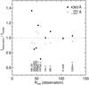 |
Fig. 1 Ratio of observed and modelled strengths of relevant [O iii] lines (indicated in the legend) vs. the temperature sensitive quantity ROIII = (I5007 + I4959)/I4363 for the 9 Galactic Halo PNe investigated by Howard et al. (1997). |
Concerning the expansion properties of PNe and their expected dependence on metallicity, the present situation is also unclear. Richer (2006) studied the expansion behaviour of PNe in Local Group galaxies and could not find any significant dependence on the metal content: the brightest PNe always have, on the average, a HWHM velocity (in the [O iii] λ5007 Å line) of ≃18 km s-1 (see also Richer 2007). A similarly low value (16.5 km s-1) has recently been found for the brightest PNe in the Virgo cluster by Arnaboldi et al. (2008). This finding is puzzling since theory predicts, as outlined above, a clear correlation of the PN’s speed of expansion with metallicity.
Because of the importance of planetary nebulae for extragalactic studies, we decided to investigate how planetary nebulae evolution depends on metallicity. In particular, we are interested in the expansion velocities of the brightest PNe and how these correlate with the metallicity of the parent stellar population, and in the question under which conditions standard photoionisation models may fail.
We start with describing the setup of our 1D radiation-hydrodynamic models in the next section, and continue in Sect. 3 with a detailed presentation of our results. In Sect. 4 we use our models to interprete the expansion velocities observed in distant stellar systems in terms of metallicity and evolutionary stage. The paper is concluded with Sects. 5 and 6. Part of the results presented in Sect. 3 can be found in Schönberner et al. (2005c).
2. The models
Our method of modelling the evolution of planetary nebulae by means of 1D radiation-hydrodynamics has been documented in previous publications and shall not be repeated here (see Perinotto et al. 2004, and references therein; henceforth called Paper I). A very detailed comparison of our models with observed nebular structures can be found in Steffen & Schönberner (2006). We add only that all hydrodynamical sequences used in this work are based on a new parallelised version of the code which also includes thermal conduction as described in detail by Steffen et al. (2008). Already existing sequences have been recomputed with this new version in order to achieve a homogeneous set of evolutionary sequences. We emphasise that, once the initial envelope structure and the central star, whose radiation field and wind represent the time-dependent inner boundary conditions, have been selected, the whole evolution is consistently determined by the hydrodynamics. We note that all the central-star models used in this work burn hydrogen, which means that the case of nebulae around hydrogen-deficient, i.e. Wolf-Rayet, central stars is thus not considered here.
Concerning the elements to be considered in the nebular envelopes, we included, next to hydrogen and helium, only the most important coolants, i.e. carbon, nitrogen, oxygen, neon, sulphur, chlorine, and argon. For each individual element up to 12 ionisation stages are taken into account. We emphasise here that ionisation, recombination, heating and cooling are treated fully time dependently, and the (radiative) cooling function for each volume element is composed of the contributions of all individual ions (see also Marten & Szczerba 1997). Our reference abundance distribution for the Galactic disk PNe, ZGD, is listed in Table 1. These abundances are the same as those used in our previous hydrodynamical computations and are, apart from carbon and nitrogen, very close to the most recent solar values (see, e.g., Asplund et al. 2009).
Distribution of the chemical abundances typical for Galactic disk PNe.
We considered in general six cases with scaled Galactic disk abundances distributions, ZGD, of C, N, O, Ne, S, Cl, and Ar, covering the range from Z = 3 ZGD to Z = ZGD/100 in steps of 0.5 dex. For simplicity, we did not consider metallicity-dependent variations of abundance ratios in this pilot study. The range of metal contents considered here covers the observed degrees of metallicities in galaxies: While giant galaxies have metal contents within a factor of 3 of the solar one, dwarf galaxies have less metals, usually about 1/10 of the solar case. The metal-poorer sequences are thought to demonstrate non-equilibrium effects more clearly. They are useful for interpreting objects with very low metallicity, like, for instance, the Galactic halo object PN G135.9+55.9 which has a mean metal content below 1/10 solar (Péquignot & Tsamis 2005; Stasińska et al. 2010; Sandin et al. 2010b).
The wind is treated in the same manner as originally devised by Marten & Schönberner (1991), but its dependence on metallicity, more correctly on the elements C, N, and O, is approximately accounted for by simple correction factors, i.e. Ṁ ∝ Z0.69 (Vink et al. 2001) and v∞ ∝ Z0.13 (Leitherer et al. 1992). The outcome is a nearly linear dependence of the wind luminosity with metallicity, 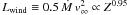 .
.
The surface of the star is always assumed to radiate like a black body, i.e. a dependence of the radiation field on the chemical composition of the stellar atmosphere is, for simplicity, not considered here. The influence of the metal content on details of the stellar evolution is expected to be small and is thus also neglected. Throughout this pilot study we employed for all metallicity cases our standard set of central-star models already used in our previous work. For the wind power calculations, the central star is assumed to have the same metal content as the nebular gas.
In every case we used the same initial envelope structures, independent of their metal content, thereby ignoring the possible influence of the metallicity on final AGB mass-loss rates and wind velocities. Our present observational and theoretical knowledge about the AGB wind properties as a function of metallicity is still too meager as to allow a more detailed description of initial configurations in terms of their metal content, although progress, theoretical and observational, is encouraging (Wood et al. 1992; van Loon et al. 2005; Wachter et al. 2008; Sandin 2008; Marshall et al. 2004; Mattson et al. 2008; Sandin et al. 2010a). There are clear indications that the wind speed is somewhat reduced at lower metallicity, but the dependence of the mass-loss rate on metallicity, and on stellar parameters, remains still unclear. It must also be noted that the particular evolutionary stage during which the remnant leaves the AGB, which is also the only relevant here, is not covered by any of these studies.
For a first assessment of the influence of the metal content, we selected a circumstellar envelope structure with initially α = 3 and v = 10 km s-1 from our set of initial models with power-law radial density profiles, ρ ∝ r−α, used in Paper II.
There it was shown that the expansion speeds seen in Galactic disk PNe with round/elliptical shapes imply radial density gradients with power-law exponents between 2.5 and >3, where the larger exponent is typical for the more evolved objects. The choice of a density gradient with α = 3 for all metallicities reflects just a compromise in order to make the model grid as simple as possible without losing its significance for practical applications.
Figure 2 illustrates the structure of the initial models in some detail. This envelope model was coupled to a hydrogen-burning post-AGB model of 0.595 M⊙ used in Paper II whose evolution in the Hertzsprung-Russell diagram is depicted in Fig. 3. The actual variations of the central star wind, based on the adopted metallicity range and the approximations introduced above, is illustrated in Fig. 4. There are two facts which emerge from this figure:
-
(i)
the wind power is very weak at the early phases of evo-lution but increases by about two orders-of-magnitude(
 ) before it decreases again with the fading central star;
 -
(ii)
even for the case of the most powerful wind (3 ZGD) its mechanical power is only a very small fraction of the photon luminosity.
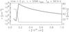 |
Fig. 2 Radial run of ion density (thick) and gas velocity (thin) for an initial nebular configuration with α = 3 density profile at age zero. The outer boundary is at r = 2.8 × 1018 cm (outside the graph). The stellar parameters are given at the panel’s top and refer to the 0.595 M⊙ post-AGB track shown in Fig. 3. Density and velocity at r = 1.0 × 1016 cm correspond to an AGB mass-loss rate of 1.3 × 10⁻⁴ M⊙ yr-1. At r ≃0.1 × 1016 cm, i.e. at the inner boundary of the envelope, density and velocity are set to the actual stellar wind properties for age zero, Ṁ = 2.5 × 10⁻⁷ M⊙ yr-1 and v = 60 km s-1 (for Z = ZGD, see text). |
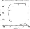 |
Fig. 3 Evolutionary path of the 0.595 M⊙ post-AGB model used for the α = 3 hydrodynamical sequences of this work. Post-AGB time marks (circles) are separated by 103 years. |
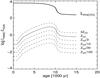 |
Fig. 4 Wind luminosities, |

The evolution of the whole system, star and circumstellar envelope, is followed across the Hertzsprung-Russell diagram towards the white-dwarf cooling path, employing our 1D radiation-hydrodynamics code. An important aspect of our hydrodynamical simulations is that we can switch off the hydrodynamics by setting the gas velocity to zero at any time in the simulation. The model is then able to settle into its equilibrium state for fixed density profile and radiation field which is reached if the electron temperature distribution remains constant throughout the entire computational domain. This kind of model corresponds then to a standard photoionisation model, but with the additional feature of having a velocity field and also a halo. We are thus able to estimate in a self-consistent manner possible systematic errors introduced by imposing equilibrium conditions for systems which are in reality influenced by dynamics.
Central stars of about 0.6 M⊙ are not luminous enough as to harbour the brightest (and thus easiest observable) planetary nebulae in a distant stellar system. We supplemented thus the already existing hydrodynamical sequences with central stars of 0.625 and 0.696 M⊙, both with Z = ZGD, which were discussed in Paper I and Schönberner et al. (2007, Paper IV hereafter), by additional sequences with other metal contents: Z = 6 ZGD (0.696 M⊙ only), 3 ZGD, ZGD/3, and ZGD/10. Except for the metallicity, the initial models are identical with those used in Paper I: α = 2 with  M⊙ yr-1, vagb = 15 km s-1. In these cases the choice of a constant mass outflow (i.e. α = 2) appears quite reasonable since these rather massive central stars have a very short post-AGB phase during which the PN remains very compact and is expected not to “see” larger variations of the circumstellar density gradient while it is expanding.
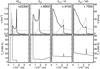 |
Fig. 5 Density, velocity and temperature profiles of models from the α = 3 sequences, selected after ≃3500 years of post-AGB evolution, and for the metallicities indicated above each panel. The central star is at the origin, and its parameters are Teff ≃ 41000 K and L = 5534 L⊙. The velocity oscillations seen in some early models are due to a temporary numerical instability in the hot bubble caused by our heat conduction routine, but have no impact on the model dynamics. Upper row: the radial profiles of heavy particle densities (thick solid), electron densities (dotted), and gas velocities (thin solid). The particle densities are normalised and must be multiplied by the factors given in the individual panels to get the true densities. Lower row: the radial run of the electron temperatures, where the dotted lines represent the equilibrium temperatures (see text for the details, and also Sects. 3.1.2 and 3.1.3). |
In order to estimate possible influences of different, albeit constant, mass-loss rates and outflow velocities on the nebular kinematics we computed several additional sequences for the 0.696 M⊙ post-AGB model with AGB mass-loss rates and wind velocities changed. For the 0.625 M⊙ post-AGB model, we computed one additional ZGD/3 sequence with Ṁagb = 0.5 × 10⁻⁴ M⊙ yr-1 and vagb = 7.5 km s-1. An overview of all the sequences used in this paper is presented in Table 2.
In the following sections we discuss in more detail implications which follow from our simulations and which are important in interpreting PNe in distant stellar systems with varying metallicities. We will thereby distinguish between the α = 2 and α = 3 model sequences.
Overview of the model sequences used in this work.
3. Results
3.1. The α = 3 sequences
Figures 5–9 illustrate how the general evolution of the model nebulae is influenced by their metal content. All sequences have the same central star of 0.595 M⊙ and start with the same initial model depicted in Fig. 2. The figures show 5 × 4 snapshots along the stellar track, viz. for five positions and for four metallicities each, Z = 3 ZGD, ZGD, ZGD/10, ZGD/100. The positions selected are at the early ionisation phase at about Teff ≃ 40000 K (Fig. 5), at the high-ionisation stage at about 100 000 K (Fig. 6), at the maximum stellar effective temperature (Fig. 7), during nebular recombination at a stellar luminosity of about 500 L⊙ (Fig. 8), and at an even lower luminosity of only 240 L⊙ after reionisation has started (Fig. 9). Note the different scaling of each individual panel within each figure, and also the different radial ranges of the figures.
An extensive discussion of the principles of PN evolution based on radiation-hydrodynamics simulations has been given in Paper I, which the reader is referred to for details. We concentrate here only on those aspects relevant in connection with the metal content of the models.
3.1.1. Structures and kinematics of the models
The upper panels of Figs. 5–9 demonstrate how structure and kinematics evolve with time. We see a strong trend with metallicity: the lower the metal content, the larger and thicker become the nebular shells and the smaller the wind-blown cavities. Responsible for this behaviour are two factors, both depending on the metal content. The first is the expansion speed of the hot, ionised gas which scales with the sound velocity  (cf. Paper II) and becomes higher at lower metallicities because of the reduced line cooling efficiency. The second is the wind power which decreases with metallicity as outlined in Sect. 2 (Fig. 4) and loses its ability to compress and accelerate the inner nebular parts. This is seen in the two metal-poor sequences where the nebular density falls off radially more gradually with a nearly linear slope (Figs. 5−8, top panels). A sharp density contrast between the rim and the shell, typical for the metal-richer models, is therefore an indication of a strong wind.
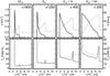 |
Fig. 6 The same as in Fig. 5 but after ≃7150 years. The 3 ZGD model is now also optically thin. The stellar parameters are Teff ≃ 100900 K and L = 4580 L⊙. |
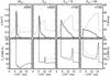 |
Fig. 7 The same as in Fig. 5 but after ≃9840 years. The stellar parameters are now Teff ≃ 146870 K and L = 1845 L⊙, corresponding to the turn-around point of the stellar track seen in Fig. 3. |
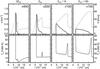 |
Fig. 8 The same as in Fig. 5 but after ≃10 530 years. The stellar parameters are Teff ≃ 131000 K and L ≃ 500 L⊙, right after the end of the recombination phase. |
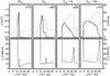 |
Fig. 9 The same as in Fig. 5 but after ≃13 850 years. The stellar parameters are now Teff ≃ 119800 K and L = 240 L⊙, typical for the reionisation stage when the nebula expands around a central star with virtually constant luminosity and temperature. |
Once the central star has passed the position of its maximum effective temperature in the Hertzsprung-Russell diagram (Fig. 7) and starts to fade quickly, also the wind power becomes progressively weaker in all cases (see Fig. 4). Figure 8 displays a moment during the recombination phase as the central star fades, and Fig. 9 a stage after reionisation has begun to dominate the inner nebular regions, forcing there the matter to develop a positive density gradient, very similar to the typical situation behind a D-type shock during the first ionisation.
Structures.
Figure 10 summarises the complete size evolution with time for all six metallicities investigated and illustrates clearly the importance of the wind interaction, given by the pressure of shocked wind (bubble) gas, as compared to the thermal pressure of nebular matter, and how these pressures change during the course of evolution. From this figure it becomes evident that wind interaction is not the main driver for the nebular expansion, although its importance becomes larger during the end phases of evolution and generally with metallicity. Rather, the expansion is initiated by thermal pressure differences, caused by photo-heating of the former neutral circumstellar gas, and continues independently of the stellar wind. Wind interaction is only responsible for compressing the inner parts of the expanding gas and preventing the shell from collapsing. This last statement is also true during the final evolution along the white-dwarf sequence: even at the lowest metallicity considered here the hot bubble is still expanding, although the stellar wind power is reduced by about one order-of-magnitude (cf. Fig. 4).
For the metal-richer models with low expansion rates and more powerful central-star winds, wind interaction becomes more important and leads to very (geometrically) thin nebular shells. However, even for the highest metallicity considered here (3 ZGD) the double-shell structure remains visible during the whole high-luminosity part of evolution. The rim succeeds in overtaking the shell not before the end of evolution (cf. Figs. 7 to 9). Neglecting photo-heating would lead to single-shell (i.e. rim only) structures in all cases.
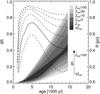 |
Fig. 10 Development of nebular sizes with time for the α = 3 sequences with various metallicities. Right ordinate: inner (Rcd) and outer radii (Rout), with the different metallicities indicated by various (overlapping) gray shades; see legend. Left ordinate: relative thicknesses, δR = (Rout−Rcd)/Rout, for the same sequences. Metallicity decreases monotonically from the bottom curve towards the top curve. |
From the observer’s point of view, only the relative sizes δR (also shown in Fig. 10) are of interest because only these can be measured distance-independently. In general, the rapid increase of δR at the beginning of the evolution reflects the dynamics of the increasing thermal pressure due to ionisation, and the decrease of δR later on is due to the increased nebular size and the stronger stellar wind. At the lowest metallicity, Z = ZGD/100, the relative sizes are close to 0.9 for most of the time, in contrast to the metal-rich models, Z = 3 ZGD, which are much more compressed and whose relative thicknesses do not exceed ≈0.6. The Galactic disk composition favours medium thick objects with δR between ≃0.5...0.7, consistent with the observations of round/elliptical PNe (cf. Fig. 6 in Paper IV).
The very different density profiles which our models develop during their course of evolution are, of course, also reflected in their surface brightness distributions. The case is illustrated in Fig. 11 where the Hβ surface brightness profiles of the models shown in Figs. 5−7 and 9 are displayed.
One sees a clear trend with metallicity: the metal-rich models (Z ≳ ZGD) develop a deep central cavity and a pronounced rim-shell structure where the shell brightness is only about 10% or less of the maximum rim brightness. The metal-poor models display a more gradual brightness decline with distance from the star, with a nearly linear (negative) slope for the lowest metallicity investigated (Z = ZGD/100). The rim-shell dichotomy known from most PNe is no longer existent. Additionally, the central cavity becomes much smaller and is nearly filled up by the projection effect.
Kinematics.
The velocity field is very similar in all cases. Once ionisation has started, the gas velocity increases nearly linearly with radius. The post-shock speed (i.e. the gas velocity immediately behind the outer edge of the nebular shell) increases with time in line with the shock acceleration (Figs. 5−9). Note that during the early stage of nebular evolution the innermost part of the ionised shell expands slower than the former AGB wind because it is decelerated by the high thermal pressure. This fact holds also during the whole evolution in the low-metallicity cases (top panels in Figs. 5−9). The post-shock speed is usually also the maximum expansion velocity within the whole nebula, with the exception of the more metal-rich models with their strong stellar winds which create dense rims and accelerates them to velocities greater than the post-shock one (Figs. 7−9). An extreme case occurs for Z = 3 ZGD where the rim becomes very dense, thin, and fast, and swallows finally the outer shell (see Figs. 7−9).
The extremely metal-poor models reach quite high post-shock (gas) velocities, up to 60 km s-1, which is twice the value achieved by the models of the 3 ZGD sequence. However, the most conspicuous features seen in Figs. 5−9 (bottom panels) are the strong shocks that these models develop with time where the shell interacts with the largely undisturbed AGB wind. The post-shock temperatures reach extremely high values, up to 50 000−60 000 K, and the whole post-shock thickness can be substantial for the most metal-poor cases. Despite of this no observed signatures are produced by these shocks because of the very low matter densities involved.
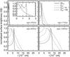 |
Fig. 11 Normalised radial surface brightness (intensity) profiles in Hβ of the models shown in Figs. 5−7 and 9. For clarity, the inset in the top left panel shows the surface brightnesses at an enlarged scale. |
The overall nebular expansion properties and their dependence on metallicity is summarised in Fig. 12 (left) where the propagation speeds, Ṙout, of the shock, which defines the outer edge of the model PNe, are plotted. Starting at rather low values the shock propagation speed increases in all cases very rapidly until the nebular shell becomes optically thin. Afterwards the shock speed (relative to the upstream flow) is determined by the density profile, ρ ∝ r-3, and the electron temperature (or sound speed) which becomes higher as the central star gets hotter and the ionising photon flux more energetic (cf. Paper II, Sect. 3.1 and Fig. 7 therein). For instance, the sudden velocity increase between 6000 and 7000 years seen in all sequences is due to the second ionisation of helium, causing a fast growth of the electron temperatures (see also Fig. 18).
As expected, the shock velocities increase with decreasing metallicity, reflecting the values of the nebular electron temperature (cf. Figs. 5−9, and also Fig. 18). The effect becomes smaller for the lowest metallicities just because also the electron temperature increase levels off somewhat (cf. Fig. 18 below). The total range of Ṙout at the end of our simulations (≃15 000 yr) is ≃55−80 km s-1 for the metallicities used here. In the 3 ZGD sequence with its powerful stellar wind we see the rim shock overtaking the more slowly expanding (38 km s-1) outer shock. This occurs at t ≃ 13000 yr when Ṙout jumps from 38 km s-1 to  km s-1 (cf. Figs. 7−9, leftmost panels).
The maxima of the gas velocities are always achieved right behind the outer shock, and are depicted in the right panel of Fig. 12. The trend with metallicity is, of course, the same as seen for Ṙout, but the absolute values are lower: starting from the shared AGB wind velocity of 10 km s-1, the gas becomes rapidly accelerated to maximum values of 32−62 km s-1, depending on metallicity. We see again the velocity jump in the 3 ZGD sequence when the shell becomes swallowed by the faster rim (cf. Figs. 7−9, leftmost panels).
Our simulations demonstrate clearly that the expansion of a planetary nebula is ruled by the electron temperature of the shell gas (cf. Paper II), and not by the wind from the central star as is predicted by the favourite theory of interacting winds put forward by Kwok et al. (1978). Wind interaction is only responsible for the shape and acceleration of the rim, i.e. the inner, bright parts of a PN, and under most conditions of our simulations the rim expands slower than the shell. With the reasonable assumption made here that the stellar wind strength decreases with metallicity, it follows that the nebular expansion of the outer shell is fastest if the wind is weakest!
The question arises whether the large variation of the expansion velocity with nebular age and metallicity can be measured. For spatially resolved objects there is the possibility to measure the fast moving matter behind the outer shock front using high-resolution line profiles taken for the central line-of-sight (Corradi et al. 2007). In the case of distant objects which cannot be spatially resolved, only the half width of the (integrated) line profile can be used. We computed therefore spatially integrated line profiles for Hβ and [O iii] 5007 Å and determined VHWHM as a measure for the nebular expansion. The results are summarised in Fig. 13.
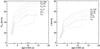 |
Fig. 12 Expansion properties of the model nebulae of the six α = 3 sequences with different metallicities vs. the post-AGB age. The five black dots along the abscissas refer to the snapshots depicted in Figs. 5−9. The initial velocities of the models are 10 km s-1 (cf. Fig. 2). Left: propagation rates of the outer shocks, Ṙout, which define the nebular sizes. The velocity jump of the 3 ZGD model at t ≃ 13000 yr marks the moment when the faster expanding rim starts overtaking the outer shock, and |

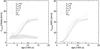 |
Fig. 13 Expansion properties as derived from the half width at half maximum (HWHM) of the spatially integrated line profiles for the same six α = 3 sequences shown in Fig. 12 vs. the post-AGB age, for Hβ (left) and [O iii] 5007 Å (right). Again, the five black dots along the abscissas refer to the snapshots depicted in Figs. 5−9. The shadowed areas indicate the thermal Doppler broadening, computed by means of the mean electron temperatures (see next section). The lower boundary refers to the models with the highest metallicity, 3 ZGD, the upper boundary to those with the lowest metallicity, ZGD/100. |
First of all, the spread in VHWHM due to the metal content is, if compared with the situation in Fig. 12, surprisingly small and partly irregular, and the increase of VHWHM with time appears to be more gentle in both lines, especially during the early phase of evolution. This can be understood as a consequence of integrating over the whole object which gives much more weight to gas elements with low velocity components along the line-of-sight if compared to the central line-of-sight case. This effect is enhanced by the density structure of the models: the gas velocity is lowest where the gas density is highest.
The HWHM velocities based on Hβ are higher than those derived from 5007 Å during the early evolution, which is due to both the different thermal line widths, indicated in Fig. 13 by the shadowed areas, and the ionisation structure: if the central star is still not very hot, the O2+ zone is confined to the inner part of the ionised region only, which is strongly decelerated by the thermal pressure (cf. Fig. 5). Thus, VHWHM as measured from the (integrated) [O iii] line starts at very low values, which are significantly below the original AGB-wind velocity of 10 km s-1 assumed here. Later on, at larger ages when the Doppler width of Hβ becomes larger than the thermal one and the O2+ zone is extending to the outer nebular edge (i.e. to the outer shock), both lines behave very similarly. In the following all velocities are from [O iii] only if not specified otherwise.
In any case, the HWHM method severely underestimates the true expansion of the nebula which is given by the propagation of the outer shock front, as seen in Fig. 12 (left panel). For instance, at age 5000 years the HWHM velocities are between 10 and 20 km s-1 while the true expansion velocities are already significantly higher, viz. between 30 and 60 km s-1! Thus, the rather large sensitivity of the nebular expansion on metallicity is almost lost by using spatially integrated line profiles. An observational test of the predicted dependence of the expansion velocities on metallicity by using an appropriate sample of PNe drawn from galaxies with different metal contents as done by Richer (2006) appears to be difficult if not impossible. We will come back to this point in more detail in Sect. 4.
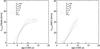 |
Fig. 14 Expansion properties as derived from the line peak separation of spatially resolved line profiles for the same six α = 3 sequences shown in Figs. 12 and 13 vs. the post-AGB age, for Hβ (left) and [O iii] 5007 Å (right). The line profiles are simulated using a central numerical aperture of 1 × 1016 cm (or 0″̣67 at a distance of 1 kpc). At low ages, the profiles are still singly peaked, and thus Vpeak = 0. The [O iii] profiles are only plotted up to model ages of about 10 000 yr because beyond this age the profiles develop a complex structure due to recombination. The five black dots along the abscissas correspond again to the snapshots depicted in Figs. 5−9. |
Applications.
It is tempting to apply our model sequences to metal-poor objects of the Milky way. The two well-known objects NGC 4361 and NGC 1360 appear especially suited for this purpose because structure and velocity informations are available from the literature. NGC 4361 belongs to the Galactic halo, while NGC 1360 is not known as an halo object but is metal-poor as well (see below). According to Méndez et al. (1992), both objects consist of a very highly excited nebula surrounding a very hot and luminous central star.
Since both objects are spatially resolved, we computed the line profiles for an aperture centred on the position of the central star (Fig. 14). At some time the lines become double-peaked, and this figure demonstrates that the expansion rates as derived from the line peak separations, Vpeak, are very similar to those derived from the integrated profiles: the dependence on metallicity is weak or even partially absent (hydrogen lines only), and the true expansion velocity is strongly underestimated as well, especially for the metal-poor cases.
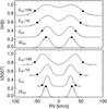 |
Fig. 15 Line profiles of Hβ (top) and [O iii] 5007 Å (bottom) computed for the models displayed in Fig. 6 for a central aperture of 1 × 1016 cm and broadened by a Gaussian of 10 km s-1 FWHM. The profiles are normalised to I = 0.25 and shifted by ΔI = 0.25 each for more clarity. Different symbols mark shock (open circles) and post-shock velocities (filled circles) of the models. |
For illustration, the (resolved) line profiles of hydrogen and [O iii] for model ages of about 7100 years (cf. Fig. 6) are rendered in detail in Fig. 15. At these ages, our models have very high nebular excitations and still luminous central stars with about 100 000 K effective temperature. The peak line emission corresponds to the denser inner regions where the emission measure is high but the gas velocity still rather modest (cf. upper panels of Fig. 6). The fast moving nebular layers immediately behind the outer shock contribute very little to the total profile and are masked by the strong emission from the denser nebular regions. This figure emphasises vividly how the real expansion of a PN is underestimated by employing the peak separation of resolved line profiles2.
Figure 15 displays also an interesting line width behaviour: the widths increase with decreasing metallicity. This is due to the different ranges of gas velocities encountered in the models (cf. Fig. 6). From the highest to the lowest metal content shown in Fig. 6, this velocity range varies from about 10 to about 44 km s-1. Also, we see for the lower metallicities a trend that the [O iii] lines have larger peak separations than the hydrogen lines. The reason is the ionisation profile of oxygen: at the evolutionary stage considered here, the O2+ concentration increases towards the outer nebular region where the velocities are higher (cf. 6th left panel in Fig. 20).
Guided by our simulations, we expect metal-poor PNe to show a more smooth or diffuse morphology without a clear-cut signature of a central cavity (or hole) and a sharp outer boundary. The surface brightness profile of NGC 4361 shows indeed neither a pronounced central cavity nor a bright, distinct rim (Monreal-Ibero et al. 2005). The metal content of this object is, on the average, ≃0.1 ZGD (Howard et al. 1997, Table 4 therein). It has also one of the highest electron temperatures, 19 300 K, of the whole Howard et al. sample (see Fig. 1). The central star has an effective temperature of ≃82000 K (Méndez et al. 1992).
In Fig. 16 we compare the Hα surface brightness of NGC 4361 with the predictions of our α = 3 models discussed here. The surface brightness is taken from a cut along the semi-minor axis in order to avoid complications due to the weak ansae seen at the poles. We conclude from the figure that only the models with a reduced metal content, Z ≲ ZGD/10, provide a quite reasonable agreement with the observation in terms of central dip and intensity profile.
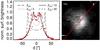 |
Fig. 16 Hα surface brightness of NGC 4361 (dots, left panel) derived from a cut along the semi-minor axis of the Hα image as indicated (right panel). We extracted this image from observations reported in Monreal-Ibero et al. (2005). The dark horizontal bars are artefacts of the VIMOS spectrograph. Also shown are the predicted Hα surface brightness distributions of models with different metal contents (see figure legend), taken from the α = 3 sequences. These models are chosen such that they match the observed size of NGC 4361, assuming a distance of 1 kpc. The model ages vary from about 6700 years (ZGD/30, fast expansion) to 9100 years (ZGD, slow expansion). |
The kinematics of our models can be tested as well: the latest velocity measurements of NGC 4361 are Vpeak(5007) = 27 ± 2 km s-1 (Muthu & Anandarao 2001) and Vpeak(Hβ) = 22 ± 5 km s-1, Vpeak(5007) = 26 ± 5 km s-1 (Medina et al. 2006). Muthu & Anandarao (2001) provide [O iii] line profiles, and the one taken from the central region of NGC 4361 (their Fig. 4c) is compared with theoretical profiles generated from the models of Fig. 16. Our metal-poorer models predict the right observed apparent expansion velocity, broader line profiles, and also Vpeak(5007) > Vpeak(Hβ).
The other case, NGC 1360, consists also of a hot (97 000 K), luminous (≈5000 L⊙) central star (Traulsen et al. 2005) and a rather smooth, extended nebula without a clear cavity/rim/shell signature (Goldman et al. 2004, Fig. 5 therein). It is reported to have a very high electron temperature (16 500 K, Kaler et al. 1990), indicative of a correspondingly low metal content (see Sect. 3.1.2). Abundance determinations for this object are rare: Kaler et al. provide only ϵ(O2+) = 7.8, while Manchado et al. (1989) found ϵ(O) > 8.2, ϵ(Ne) > 7.6, ϵ(Ar) = 5.8, which are, however, based on an electron temperature of only 10 000 K. A higher electron temperature as mentioned above would result in correspondingly lower abundances. Traulsen et al. (2005) provide also photospheric abundances of the central star which, converted to the notation used here, are: ϵ(C) = 8.3, ϵ(N) = 7.7, and ϵ(O) = 8.3. Thus, NGC 1360 is certainly also a metal-poor object (compare with the Galactic disk abundances in Table 1).
García-Díaz et al. (2008) measured recently the apparent expansion of NGC 1360 by means of high-resolution echelle spectrograms: Vpeak(Hα) = 26 km s-1, consistent with older measurements of 24 km s-1 by Goldman et al. (2004). Again, the agreement with the predictions of our models for this particular stage of evolution (≃7100 yr, Fig. 14) is satisfying. We repeat that the real expansion rate of both objects is expected to be considerably higher, viz. up to a factor of about two (cf. Fig. 12, left panel, and Fig. 15).
Goldman et al. (2004) determined also an elliptical spatio-kinematic model of the nebula structure of NGC 1360, based on the position-velocity ellipse and the surface-brightness distribution. The basic result is that the gas density falls off outwards, while the gas velocity increases outwards, i.e. the density (or surface brightness) is highest close to the central star where the expansion velocity is lowest. The fastest expanding shell has ≃35 km s-1 at the equator and ≃70 km s-1 at the pole. The density, velocity, and surface brightness profiles predicted by our metal-poorer models (Fig. 6, top panels, and Fig. 11) are in agreement with the mean properties of the Goldman et al. model of NGC 1360.
García-Díaz et al. (2008) constructed a dynamical (2D) model including magnetic fields, but their main point was the following: they assumed that the stellar wind has stopped shortly after the formation of the PN (i.e. after 1000 years) and followed the dynamical evolution with a collapsing hot bubble for additional 10 000 years. Despite the authors’ claim that their model “successfully reproduce many of the key features of NGC 1360”, we note following inconsistencies:
-
1.
the final nebular model at t = 11000 yr inFig. 6 of García-Díazet al. (2008) shows a positivegradient for both the velocity and density: the outer fastest layersare also the densest, i.e. the model islimb-brightened (except at the poles), which is in clearcontradiction with the observations;
-
2.
despite the long simulation time of 11 000 years, an evolution of the star is obviously not considered. The stellar model envisaged is rather massive (≃0.75 M⊙, Vassiliadis & Wood 1994) and crosses the HR diagram within only about 1000 years and fades thereafter, accompanied by a drop of wind power (cf. Figs. 3 and 4). After 11 000 years, the model’s luminosity is then only ≈100 L⊙.But presently the central star of NGC 1360 is still a high-luminosity object with several 1000 L⊙, luminous enough to sustain a radiation-driven wind which, because of the low metallicity, may be too weak for developing spectroscopic signatures.
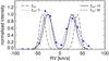 |
Fig. 17 Observed central 5007 Å line profile of NGC 4361 (connected crosses) as measured by Muthu & Anandarao (2001) compared with the profiles generated from the models used in Fig. 16. As in Fig. 15, the theoretical profiles are computed for a central aperture of of 1 × 1016 cm and then broadened by a Gaussian of, now, 12 km s-1 FWHM. |
We emphasise at the end of this discussion that models taken from the α = 3 sequences displayed in Figs. 5 to 9 can explain the (mean) properties of two rather well-known metal-poor objects very successfully, although they were not designed to fit any particular object! Furthermore, according to our models, it is not justified to conclude, just from the non-existence of an apparent central hole in the surface brightness distribution of a PN, that the central-star wind has already stopped and that the nebular gas is now falling back onto the star. Rather, a detailed analysis of the density and velocity structure of the object in question appears to be mandatory in order to decide whether a deceased central-star wind is responsible for a more smooth or diffuse appearance of a PN, or whether we observe a low-metallicity system with a weak central-star wind and a more extended nebular structure.
We acknowledge, however, that our spherical models are certainly too simple in order to provide detailed models of the objects discussed in this section. Important further ingredients are, e.g., inhomogeneities, jets, and other means that impose departures from sphericity. We note also that magnetic fields have been detected in NGC 1360 by Jordan et al. (2005), but whether they are really important in shaping NGC 1360, as believed by García-Díaz et al. (2008), must be seen in the future when more realistic simulations become possible.
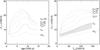 |
Fig. 18 Mean [O iii] electron temperatures, computed according to Eq. (1), for all α = 3 nebular models as function of the post-AGB age (left) and stellar effective temperature (right). In the right panel, the models are only plotted until maximum central star temperature (corresponding to a post-AGB age of ≃9800 years in the left panel) in order to avoid confusion due to overlapping lines. The grey area depicts approximately the region occupied by the hydrodynamic models presented in Paper I and Paper IV which have all Z = ZGD, but various initial conditions and central stars. |
3.1.2. Electron temperatures
We computed the mean electron temperatures of the models according to 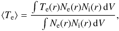 (1)with Ne(r) being the electron number density, Ni(r) the O+2 number density, Te(r) the electron temperature, and dV the volume element. The upper boundary for the volume integration is set at the outer shock front; the halo (=ionised former AGB wind) is thus excluded. In passing we remark that Eq. (1) corresponds in practice to an emission weighted mean of the electron temperature, in contrast to the usual meaning of a mean value. Differences are only expected for cases with radial temperature gradients and/or strong shocks as seen in the late, metal-poor models of Figs. 5−9.
The determination of the mean electron temperature from the model structure by using Eq. (1) is convenient but different from the one used in practice if the nebular structure is not known. The alternative is to compute first the (total) line strengths from the model and to apply then, e.g., Eq. (5.4) of Osterbrock (1989) to get a volume averaged TOIII from the ratio ROIII. Provided the collision strengths are correct, both methods should give the same result. We performed a test using two sequences with rather extreme metallicities, viz. with ZGD and ZGD/100. In the first case we found always |⟨ Te ⟩ −TOIII| ≲ 60 K, in the second |⟨ Te ⟩ −TOIII| ≲ 170 K. Thus the (relative) differences between both methods are less than about 1%, and the temperature determination according to Eq. (1) provides an excellent value for TOIII.
The run of the mean electron temperature, ⟨ Te ⟩ , is displayed for all α = 3 sequences in Fig. 18, and we see, as expected, a strong temperature dependence on metallicity. The first rapid increase of the mean electron temperature is, of course, due to hydrogen ionisation. Already at this stage one sees clearly how rapidly the electron temperature increases with decreasing cooling efficiency. Then the temperatures increase further as the central star becomes hotter and its photons more energetic. The second temperature “jump” after about 5000 years is due the second ionisation of helium, providing additional energy input to the gas.
Because the effective temperature decreases once the central star begins to fade rapidly at an age of about 10 000 years (cf. Fig. 3), the electron temperature in the nebula must drop accordingly. This is clearly seen in Fig. 18 (left) for the more metal-rich models in which expansion cooling is not very important. However, the relation ⟨ Te ⟩ −Teff differs between the stellar high- and low-luminosity branch because of differences in the nebular ionisation: at a given stellar temperature, the nebular ionisation is higher and line cooling lower at the high-luminosity branch. Hence, the electron temperature along the low-luminosity branch of evolution is significantly below that along the corresponding high-luminosity branch, independently of non-equilibrium effects.
An interesting effect is seen for the more metal-poor sequences (Z < ZGD/3) which expand faster and become hence more dilute: here expansion cooling becomes relevant during more advanced evolutionary stages and forces the nebular electron temperature to drop at progressively lower stellar temperatures (cf. Fig. 18, right panel). A more detailed discussion about expansion cooling is given in Sect. 3.1.4.
Note that the interplay between line and expansion cooling, and their relative importance, depend sensitively on gas density and expansion velocity. It is, however, clear from our simulations that a low metal content results in high electron temperatures because of less line cooling, leading consequently to faster expanding and more diluted nebulae which are then prone to departures from thermal equilibrium. The grey region seen in the right panel of Fig. 18 delineates the approximate area occupied by ⟨ Te ⟩ of all the hydrodynamical sequences previously used in Paper I and Paper IV, which have very different combinations of initial AGB-envelope configuration and central star, but all with the ZGD composition. These models sequences demonstrate that only a low metal content can be responsible for unusually high electron temperatures in nebular envelopes.
We note also that the conspicuous shock regions seen in Figs. 5−9 do not contribute to the electron temperatures, although the post-shock temperatures become very high and are included in the integration according to Eq. (1). The reason are the low ion (i.e. O2+) densities, giving these outer shock regions only a minute weight in the integral.
3.1.3. Comparisons with equilibrium models
With the computation of equilibrium models (with respect to ionisation and thermal energy) at selected positions along the evolutionary path we have a unique tool to investigate under which circumstances non-equilibrium effects may become important.
Electron temperatures.
In equilibrium, the electron temperature is determined by the balance between radiative heating and cooling processes: because heating is mainly due to ionisation of hydrogen and helium, and because generally a significant contribution to cooling comes from line radiation of heavier ions, the models must become hotter with lower metallicities. During the course of evolution, the electron temperatures generally increase because the stellar photons become more energetic (see discussion in Sect. 3.1.2 above). At low metallicity the contribution of radiation from collisionally excited metal ions is reduced, and line cooling is limited mainly to free-bound emission of hydrogen and helium. Hence, cooling by expansion becomes more important for the energy balance, thereby limiting the electron temperature increase. This process is favoured by the larger expansion rates of the low-metallicity models. See Sect. 3.1.4 for more details.
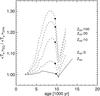 |
Fig. 19 Ratios between electron temperatures of equilibrium (eq) and dynamical (dyn) α = 3 models with different metal contents are plotted versus post-AGB age. The filled dot on each curve indicates the position of maximum stellar temperature. The sharp local minima of the temperature ratios occur during nebular recombination while the central star fades rapidly (cf. Figs. 3 and 8). See text for details. |
The bottom panels of Figs. 5−9 display both the dynamic and the equilibrium electron temperatures. The close correspondence between the dynamic and equilibrium electron temperatures seen in the metal-rich models during the horizontal evolution across the HR diagram indicates that the gas heating time scales are much smaller than the stellar time scales for heating due to the ionisation of hydrogen and helium (see also Marten 1995). This statement holds independently of the metal content of the gas, and any deviations seen at later stages and/or for lower metallicities must be due to the dynamics. As expected, the temperature differences become largest for the models with the lowest metallicity, and hence lowest line cooling, and can reach up to about 10 000 K in extreme cases.
Figure 19 gives a more detailed illustration of how the deviations between dynamical and equilibrium models, measured by their mean O2+ electron temperatures, develop with time (or evolutionary stage of the central star). One sees that, in general, the differences increase with evolution, and they become large for the metal-poor models: under equilibrium conditions the electron temperatures can be higher by up to 30% in the metal-poorest case of Fig. 19.
During the fast luminosity drop of the central star between 10 000 and 11 000 years (cf. Figs. 3 and 8) one sees in Fig. 19 that the mean temperature ratio eq/dyn becomes equal to or even slightly lower than unity. Line cooling increased by recombination is not sufficient to explain this; rather we see a typical time-scale effect: the fading time scale of the star,  , becomes for about 300 years as short as 400 years, which is quite comparable to the cooling time scale of the diluted nebular gas. Thus, it may well happen that the electron temperature in thermal equilibrium comes close to or even falls below non-equilibrium value because the latter cannot keep pace with the fading central star. After stellar fading is completed (at ≈11000 years in Fig. 19), the previous differences of electron temperatures are restored quickly.
A few comments concerning the halo, i.e. the still rather undisturbed but ionised AGB material ahead of the outer shock front, are in order here. Marten (1993a, 1995) showed that, because of its rather low density, the halo gas is especially prone to non-equilibrium conditions, even with solar metal content. Generally one can say that the energy balance of the inner, denser halo regions of young PNe are controlled by line cooling, while in the outer, less dense regions expansion cooling prevails.
Right after the passage of the ionisation front, the halo becomes quite hot and cools then slowly down, with a (local) time scale ruled by the local density. Such temperature profiles can be seen for the metal-rich models in Figs. 6−9 (lower leftmost panels) which are very compact and become optically thin quite late when the central star is already quite hot (Teff ≃ 40000−42200 K).
The situation is different for the other models. They become optically thin earlier with cooler central stars (Teff ≃ 33000−35000 K), and the halo is not so much heated in the first place. According to Marten (1995) the mean heating time scale of the halo gas can be comparable to or even larger than the stellar heating time scale due to ionisation of hydrogen and helium. Under such condition the dynamical haloes remain always quite cool during the whole evolution, in contrast to the equilibrium condition. In general, the halo temperatures follow the trend of the main nebulae and become hotter with decreasing metal content. In the extreme cases the equilibrium electron temperatures exceed locally 40 000 K (cf. Figs. 6−7).
 |
Fig. 20 Radial ionisation structures for hydrogen, helium, carbon, nitrogen, oxygen, and neon of the Z = ZGD/10 model presented in Fig. 7. The two top panels show again the underlying nebular structures: densities (ions = thick, electrons = dotted), gas velocity (thin), both left, and electron temperatures (dynamical = solid, equilibrium = dotted, right). The shadowed vertical strip marks the region occupied by the shell’s leading shock in all panels. The ionisation fractions, X, are labelled as follows: dotted = neutral (hydrogen and helium only), short-dashed = 1st ionisation, dash-dotted = 2nd ionisation, dash-dot-dot-dot = 3nd ionisation, long-dashed = 4th ionisation, and dotted = 5th ionisation (except for hydrogen and helium), and are displayed in the left panels for the dynamical model (Xdyn). The ionisation fractions are omitted inside the contact discontinuity (r < 3.5 × 1017 cm) in order to avoid confusion. On the right, the ratios between the equilibrium (eq) and dynamical case (dyn) are shown. Only the ratios of major ionisation fractions, which are seen also in the left panels, are rendered for clarity. |
Ionisation structure.
Although a PN might well be out of thermal equilibrium because of dynamics, ionisation equilibrium is generally rather well established. During the high-luminosity phase as the object crosses the HR diagram, ionisation dominates over recombination in the ionisation equations, and the nebular ionisation quickly adjusts to the stellar ionising photon flux. Our hydrodynamical models are thus always close to ionisation equilibrium. An exception is only possible for a brief period during the rapid stellar fading when the ionisation time scale may become larger than the recombination time scale (e.g., of hydrogen), and provided the latter is then comparable to or larger than the fading time scale of the star. Ionisation equilibrium is quickly re-installed later when the stellar luminosity evolution slows down on the white-dwarf cooling track.
As an example we compare in Fig. 20 the ionisation properties of the dynamical and the thermally relaxed ZGD/10 model from Fig. 7. We selected this model because it is far evolved and has a very high degree of excitation because of the very hot and luminous central star. The metallicity chosen, ZGD/10, is typical for very metal-poor populations, e.g., in the Galactic halo and in some distant stellar systems.
One sees in Fig. 20 that behind the shock (r ≲ 12 × 1017 cm), i.e. in the nebula, the ionisation structures of both model types are very similar but not identical. The deviations seen in some cases are up to 10 to 15% for main ionisation stages. These obvious deviations from a pure photoionisation equilibrium are due to collisional ionisation whose contribution, albeit quite small, increases with electron temperature. Different electron temperatures lead then consequentially also to small differences of the ionisation.
The situation is demonstrated for hydrogen and helium (2nd and 3rd right panels in Fig. 20). In the dynamical case, hydrogen and helium are less ionised both in the halo and the nebula proper. The departures of the ionisation fraction ratios from unity follows closely the difference between, or ratio of, the electron temperatures. Only during the passage through the of the high-temperature shock region the ionisation of hydrogen and helium becomes temporarily larger than in equilibrium because of enhanced collisional ionisation.
Note also that for the particular, very diluted model shown in Fig. 20 where the central star is very hot and still quite luminous, doubly-ionised oxygen which is so important for analysing nebular spectra is only a minority species.
Because of its lower density, the halo, i.e., the matter ahead of the shock at r ≳ 14 × 1017 cm, shows generally a larger degree of ionisation than the main nebula. For instance, the fraction of neutral hydrogen is about 10-4 in the halo, but about 10-3 in the nebula. Similar differences occur for the fraction of singly ionised helium: about 4 × 10⁻³ in the halo and about 4 × 10⁻² in the nebula. The heavier elements show the same behaviour (cf. left panels of Fig. 20, for N, O, and Ne).
It is also seen in Fig. 20 (right panels) that the halo region is also prone to deviations from the ionisation/recombination equilibrium: the haloes of the dynamical models have lower degrees of ionisation than in the corresponding equilibrium cases (cf. nitrogen, oxygen, and neon in Fig. 20), indicating that the gas ionisation time scale exceeds the stellar ionisation time scale. The reason is the small fraction of high-energy photons which are able to sustain such a high ionisation. Thus, the ionisation time scale becomes the longer the higher the gas ionisation. Additionally, ionisation by electron collisions is more important in the cases of the very high halo temperatures. In equilibrium, the 5th ionisation (N, O, and Ne) appears to be the preferred one. After the halo gas becomes swallowed by the shock recombination brings the gas immediately back to a lower degree of ionisation very close to equilibrium conditions.
The generally higher degree of ionisation within the haloes leads to a lower line cooling efficiency which in turn is responsible for the quite substantial temperature jumps across the nebula/halo boundaries, i.e. the shock, seen in the equilibrium models (top right panel of Fig. 20).
3.1.4. Line vs. expansion cooling
Here we want to discuss in more detail the relevance of the different cooling processes encountered in our models. The nebular gas is heated by ionisation and cooled by line radiation from free-free, bound-free (recombination) transitions, and from collisionally excited atomic or ionic levels3. Additionally, the gas is subject to dynamical processes leading to cooling by expansion or heating by compression.
In standard photoionisation modelling it is implicitly assumed that dynamics is unimportant, hence the thermal balance of the heated nebular gas is controlled by line radiation only. Since the most important coolants are metal ions, the cooling function decreases with metallicity until radiation from hydrogen and helium prevails. Furthermore, radiation cooling depends on gas density squared, leading to a reduction of the cooling efficiency also because the nebula expands with time. In contrast, cooling by expansion depends only on the gas velocity.
Under adiabatic conditions, the total change of thermal energy content of a volume element, U (in erg cm-3), with time is given by 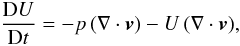 (2)where v is the flow velocity and p the thermal pressure (see Eq. (A11) in Marten & Szczerba 1997). The term p(∇·v) is the usual local source (sink) term due to compression (expansion). The second term of the right-hand side of Eq. (2) accounts for the change of the volume of a gas parcel with time, i.e. a gas parcel becomes expanded or compressed while streaming.
It is more convenient to follow a mass element and rewrite Eq. (2) using the thermal energy per mass, e = U/ρ (in erg g-1), as 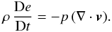 (3)Note that only in case of constant density, ρDe/Dt = DU/Dt follows.
Introducing p = nkBTe, with n being the total particle density (ions + electrons), kB the Boltzmann constant, and Te the electron temperature, we get from Eq. (3) in spherical coordinates ![Mathematical equation: \begin{equation} \rho\,\frac{{\rm D}e}{{\rm D}t} = - n\,k_{\rm B} T_{\rm e} \left \{\frac{\partial v}{\partial r} + \frac{2v}{r} \right \} \quad \rm [erg~cm^{-3}~s^{-1}]. \label{E.exp} \end{equation}](/articles/aa/full_html/2010/15/aa13427-09/aa13427-09-eq165.png) (4)Estimating possible dynamical effects demands knowledge of the density and the velocity structure of the object in question, both of which are difficult – if not impossible – to get observationally. One may use the measured line width VHWHM which, however, is an unsuitable choice: this velocity value is (i) much lower than the real expansion speed and (ii) is constant (i.e. the velocity gradient disappears), leading to a substantial underestimate of expansion cooling. The assumption of a constant electron density may also introduce an uncertainty. It remains the likewise difficult choice of a – distance dependent – radius range. One could determine the radial extent of an object from a model, or select the outer edge of the nebula. In the latter case, an additional systematic underestimate of the expansion cooling would result.
(4)Estimating possible dynamical effects demands knowledge of the density and the velocity structure of the object in question, both of which are difficult – if not impossible – to get observationally. One may use the measured line width VHWHM which, however, is an unsuitable choice: this velocity value is (i) much lower than the real expansion speed and (ii) is constant (i.e. the velocity gradient disappears), leading to a substantial underestimate of expansion cooling. The assumption of a constant electron density may also introduce an uncertainty. It remains the likewise difficult choice of a – distance dependent – radius range. One could determine the radial extent of an object from a model, or select the outer edge of the nebula. In the latter case, an additional systematic underestimate of the expansion cooling would result.
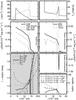 |
Fig. 21 The effect of dynamical/expansion cooling as described by the source/sink term p(∇·v) for the ZGD/10, α = 3 model shown in Fig. 7 where the central star has gained its maximum effective temperature (see the track in Fig. 3). Top row: model structure with particle densities and flow velocities (left, ions = thick solid, electrons = dotted, velocity = thin solid) and temperatures (right, dynamical = solid, equilibrium = dotted). The shadowed vertical strip indicates the thickness of the outer shock region. Second row: different contributions of line cooling (left) and dynamical cooling (right), as indicated in the legends, both based on the equilibrium temperature. The right panel with the two hydrodynamical terms (∂v/∂r and 2v/r) is “mirrored” at the horizontal axis in order to show also heating due to compressions if ∂v/∂r becomes negative (shock front and halo/upstream region). Note that no cooling terms are plotted for the hot bubble, i.e. inside the contact discontinuity at ≃3.5 × 1017 cm. Bottom left (shadowed): total cooling (line + hydro) to line cooling, taken from the middle panels (thick solid) and for models with the same evolutionary time but with other metallicities (see legend). Note the different radius ranges covered by the models: the inner boundaries are set by the respective contact discontinuities, and the vertical “double” lines mark the outer shock regions where heating by compression prevails. Bottom right: ratio between adiabatic cooling using Eq. (4), with the model data displayed in the top panels (hydro) and using various approximations (approx), always based on the equilibrium electron temperature: mean of total particle density of 40 cm-3 and fixed outer radius Rout = 1.4 × 1018 cm (dash-dotted), the (same) mean density but a variable radius (dotted), variable density and fixed outer radius (dashed), and finally variable density and radial coordinate (solid). In all cases, the model velocity VHWHM = 40 km s-1 is used. |
The whole situation is illustrated in Fig. 21 for an evolved nebular model of the α = 3 sequence with ZGD/10 where the central star is at its maximum effective temperature (cf. Figs. 7 and 20). We selected this metallicity because we have previously seen that at this value hydrodynamical effects become significant for more evolved and diluted models. This figure allows both a detailed insight into the behaviour of the different cooling processes and an assessment of dynamical cooling.
We employed the equilibrium temperature profile for estimating hydrodynamical effects since this is the case if one uses a photoionisation code. For this metallicity and ionisation stage line cooling is dominated by free-bound transitions throughout the entire nebula (Fig. 21, middle left). The largest contribution to cooling from collisional excitation comes from neutral hydrogen, albeit its fraction is very small (≈10-3). Expansion contributes to the total cooling everywhere, except at the shock where the gas is heated considerably by shock compression (Fig. 21, middle right). Expansion cooling makes up for about 35% of the line cooling in the outer regions of the model immediately behind the shock where the expansion is the fastest and the density the lowest. This extra cooling is responsible for the temperature difference of a few thousand degrees seen between the dynamical and equilibrium model in the right top panel of Fig. 214.
The bottom left panel of Fig. 21 compares the relative importance of hydrodynamical cooling for additional models of the α = 3 sequences. All these models are of the same age, which corresponds to maximum stellar temperature (cf. Fig. 7). For these models, the contribution from hydrodynamics must be considered if the metallicity drops below 1/3 to 1/10 of the Galactic disk (or solar) value. Furthermore, we also see that the hydrodynamic cooling in the metal-rich models is restricted to outer regions. In their inner regions, i.e. the rims, a negative velocity gradient indicates compression which, at least partly, compensates the second term within the curly brackets of Eq. (4). This behaviour disappears with decreasing metallicity. One can also see that the shapes of the curves representing the ratios of total cooling to line cooling correspond directly to the electron temperature differences between the dynamical and equilibrium models in Fig. 7.
The bottom left panel of Fig. 21 also shows that for all these very advanced models the dynamics is important for the thermal balance of the halo regions: expansion cooling is larger than line cooling for all shown models, although the former is quite small because of the low flow velocities and a slight compressional contribution from a tiny negative velocity gradient (see top left panel and right panel of the second row, both for r ≳ 14 × 1017 cm).
The right bottom panel of Fig. 21 illustrates the errors made when Eq. (4) is used with various simplifications. Generally, the dynamical cooling is always underestimated, in one case locally up to a factor of ten! The best result is achieved by using the correct density and radius variables of a model (provided they are available) together with the VHWHM velocity. Since the electron temperature is fairly constant through the whole nebular structure, an empirical mean value is a reasonable choice for all cases. The error figures found here are model-dependent and cannot be generalised.
We conclude from the discussion in this section that any method to estimate empirically the contribution of dynamics to the total cooling function from an otherwise static model, as done by Stasińska et al. (2010) in their study of the metal-poor PN G135.9+55.9, will not provide a sound result. These authors used Eq. (4) with the assumption ρDe/Dt = DU/Dt, but omitted the velocity gradient by setting v(r) ≡ VHWHM and r ≡ Rout (cf. right bottom panel of Fig. 21). Only from full dynamical simulations one can get hold of the correct contribution of dynamics to the heating/cooling balance of a nebular model.
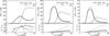 |
Fig. 22 Top panels: run of line strengths (relative to Hβ = 100) of three collisionally excited oxygen lines, O iv] λ 1402 Å, [O iii] λ 5007 Å, and [O iv] λ 26 μm, with stellar temperature for three α = 3 model sequences, viz. Z = ZGD (left), Z = ZGD/10 (middle), and Z = ZGD/100 (right). The evolution is only shown until maximum Teff in order to avoid confusion. Note the different ordinate ranges. Bottom panels: line strength ratios Leq/Ldyn. The small scatter seen for the λ 1402 Å ratio in the metal-rich model is due to numerics. |
3.1.5. Line strengths
The temperature differences between dynamical and equilibrium models have, of course, consequences for the line emission, especially for that of the collisionally excited lines, as has been already demonstrated by Schönberner et al. (2005c). The effect is again illustrated in Fig. 22 for three lines of oxygen, in the UV (O iv] λ 1402 Å), the optical ([O iii] λ 5007 Å), and the IR region ([O iv] λ 26 μm). The trend is as expected:
-
in equilibrium the models show a tendency to have always higherline strengths, in line with the temperature difference to thedynamical case;
-
the differences increase with evolution (or stellar temperature) and decreasing metallicity; they can, however, be totally neglected for more normal or metal-rich compositions (cf. Fig. 22, left bottom panel);
-
the relative differences of line strengths between both types of models are the largest for UV lines and the smallest in the infrared. The optical lines behave intermediately. At the lowest metallicities considered here (ZGD/100), O iv] λ 1402 Å can be off by about 250% if thermal equilibrium is assumed. The corresponding value for [O iv] λ 26 μm is only about 30% (cf. Fig. 22, right bottom panel).
Note that the main reason for the differences of line strengths between equilibrium and dynamical models is the electron temperature because we found only very small deviations from ionisation equilibrium (cf. Sect. 3.1.3 above). We repeat that the discrepancies found here are highly dependent on structure and expansion properties of the model and should be regarded as indicative only.
We see also in Fig. 22 that the expected changes of line strengths with the corresponding abundances is partly compensated by the electron temperatures. For instance, at medium stellar temperatures when O2+ is the main ionisation stage and the electron temperatures increase with decreasing Z (cf. Fig. 18), the line strength of 5007 Å decreases roughly with 0.5ϵ(O) only. At high excitations (Teff ≳ 100000 K) when most oxygen is O3+, the electron temperatures of very metal-poor (dynamical) models become nearly independent of metallicity (Fig. 18), and hence the strength of, e.g., 26 μm varies proportional to ϵ(O).
Our metal-poor models are well suited to address the question of how one can determine the chemical composition of metal-poor PNe if conventional plasma diagnostics is not feasible because of lack of suitable lines, as is the case for PN G135.9+55.9. One is then left with photoionisation modelling for constraining, e.g., the oxygen abundance, as has been shown extensively and illuminatingly by Péquignot & Tsamis (2005). According to these authors, the oxygen abundance of PN G135.9+55.9 is likely not below 1/30 of the solar value, assuming a stellar temperature of ≃130000 K5.
However, for a highly-excited PN like PN G135.9+55.9 the oxygen content can best be estimated by using, e.g., the 26 μm line whose strength depends only weakly on the electron temperature and its uncertainties (cf. Fig. 22). The optical oxygen line at 5007 Å cannot be recommended because its higher sensitivity to the electron temperature, especially if the stellar temperature is above 100 000 K. Ultraviolet lines of highly ionised elements, such as O iv] λ 1402 Å, should not be used at all for abundance studies because these lines depend strongly on electron temperatures at nearly all stellar temperatures.
We conclude from this discussion that the use of photoionisation models assuming thermal equilibrium is not adequate for objects with a diluted nebula and a very hot central star (i.e. for highly excited objects as represented by our models) and with reduced metallicity because of incorrect physical assumptions. Note that departures from thermal equilibrium depend only on the gas properties regardless of the nature of the central ionising object. Of course, this will become evident only if the restriction to one wavelength region (e.g. the optical) is relaxed. Our models show that, for UV lines, departures from equilibrium may become a problem already for Z ≲ ZGD/3. They suggest also that the neglect, or a too simple consideration, of dynamical effects in the modelling of a metal-poor and highly excited PN, as done in the recent study of PN G135.9+55.9 by Stasińska et al. (2010), becomes problematic.
Based partly on new spectroscopic material, Sandin et al. (2010b) performed an abundance study of PN G135.9+55.9 taking full advantage of the dynamical models discussed here. For the details, the reader is referred to the cited paper.
3.1.6. The Milky Way halo PNe
In this context it is interesting to see how the known Galactic halo PNe fit into our grids of mean electron temperatures vs. stellar effective temperatures or ages of the simple hydrodynamical α = 3 models as shown in Fig. 18 and whether hydrodynamical effects are discernable. As ages of the halo PNe are not known, and their stellar temperatures are too uncertain, we used the nebular excitation as given by the relative strength of He ii λ 4686 Å for a proxy of the evolutionary status of both the objects and models.
The result is seen in Fig. 23 where the mean [O iii] temperatures are now plotted against L(4686)/L(Hβ) instead. We compared our models (also in equilibrium) with both the electron temperatures from detailed nebular analyses by means of photoionisation models as provided by Howard et al. (1997) and with the corresponding temperatures derived directly from the observed temperature sensitive [O iii] line ratios6. K 648 and DdDm-1 are omitted because they do not show a He ii λ 4686 Å line.
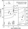 |
Fig. 23 Mean nebular [O iii] electron temperatures vs. nebular line ratio L(4686)/L(Hβ) for the dynamical α = 3 sequences from Fig. 18 (dotted in thermal equilibrium). Again, the sequences are only plotted until maximum stellar temperature in order to avoid confusion. The circles give the corresponding positions of the Halo PNe: filled circles are based on the observed [O iii] lines, open circles are results of detailed analyses using photoionisation models (Howard et al. 1997). The inset renders an enlarged view of the region around L(4686)/L(Hβ) ≃ 1. |
Neglecting for the moment M2-29, the following emerges from Fig. 23:
-
compared with the simulations, the observed mean electrontemperatures suggest nebular abundances between ZGD/3 < Z < ZGD/30, which is inreasonable agreement with the spectroscopic analyses in theliterature (cf. Table 4in Howardet al. 1997);
-
on average, discrepancies between observed and modelled temperatures increase with excitation: they are less than 1000 K at L(4686)/L(Hβ) ≃ 0.1, but up to 3500 K at the highest excitation, L(4686)/L(Hβ) ≃ 17. This is consistent with the predictions of our model sequences if one neglects the (unexplainable) fact that for the 3 objects with medium 4686 Å line strengths the Howard et al. (1997) temperatures are below the temperatures derived from the observed line strenghts, while they are above for the 3 objects with the highest excitations.
Because abundances derived from collisionally excited lines depend strongly on the electron temperature, one is tempted to say that the use of standard photoionisation models cannot be recommended for cases where non-equilibrium (i.e. dynamical) effects become important. This statement may become applicable already at metallicities below about one third solar, for very diluted and rather fast expanding nebulae.
For M2-29 with its only moderate excitation the discrepancy between observed (from ROIII) and modelled temperatures is the largest, ≃8000 K, and at disturbing variance with the model predictions. First of all, the photoionisation models of Howard et al. are based on the incorrect [O iii] λ4363 Å line strength of 15 (Hβ = 100) which is the undereddened value (cf. Peña & Torres-Peimbert 1991, Table 2A). We used in Fig. 23 the dereddened value of 19.5 instead, leading to an electron temperature of 24 000 K which is then the highest in the Howard et al. (1997) sample of Galactic halo PNe. The photoionisation model of Howard et al. (1997) predicts a λ4363 Å line strength of 11 only instead of the assumed value 15, which would correspond to an electron temperature of about 20 000 K.
Because of the high electron temperature, the plasma diagnostics of Peña & Torres-Peimbert (1991) leads to a lower metallicity for M2-29 than claimed by Howard et al. (1997): a metal depletion by factors between 20 and 30. Still, the problem of M2-29’s too high electron temperature remains a mystery: at its moderate excitation this high electron temperature would suggests a metallicity well below ZGD/100, which is not observed. In this context it is interesting to note that Hajduk et al. (2008) claimed recently that the nucleus of M2-29 consists of a binary system with an eclipsing disk.
3.2. The α = 2 sequences
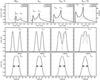 |
Fig. 24 Composite figure showing one snapshot taken at maximum 5007 Å brightness along each of the four 0.625 M⊙ sequences (α = 2), with the metallicities indicated over the panels. Details of the models are listed in Table 3. Top panels: structures of the models: run of ion density (thick solid line), flow velocity (thin solid line), and electron temperature (dotted line) with radius. Densities and temperatures are normalised and must be multiplied with the factors given in each panel. The radial positions, Rout, of the nebular outer shock and of the rim, Rrim are also marked in each panel. The central star is at r = 0 cm. The electron temperature spikes seen at larger radii are caused by the ionisation fronts, and the jumps at the inner nebular edges mark the positions of the contact discontinuity/conduction fronts. Middle panels: normalised spatially resolved [O iii] 5007 Å and thermally broadened line profiles (dotted line) as seen through a central numerical aperture with a diameter of 1 × 1016 cm (corresponding to 0″̣67 at 1 kpc), and additionally broadened by a Gaussian of 10 km s-1 FWHM (solid line) in order to simulate a typical instrumental broadening. The maximum velocity behind the outer shock at Rout, Vpost, is indicated by vertical dashed lines. Bottom panels: [O iii] 5007 Å line profiles as integrated over the whole nebula (dotted line), and additionally broadened by a Gaussian of 10 km s-1 FWHM (solid line). Two vertical dashed lines in each panel indicate the HWHM and the shock velocity, Ṙout, respectively. |
Recently we showed in Paper IV that the bright cutoff of the PNLF can be explained by nearly optically thick nebulae around central stars with masses slightly above 0.6 M⊙. However, in Paper IV we only assumed a metal content that is typical for Galactic disk objects. We thus continue our work with investigating the properties of model nebulae around more massive (and much faster evolving) central stars, 0.696 M⊙ and 0.625 M⊙, and with different metal contents, 3 ZGD, ZGD, ZGD/3, and ZGD/10. This is also the mass range of interest in observations of very distant stellar populations because there only the most luminous nebulae are accessible for more detailed studies (see, e.g., Arnaboldi et al. 2008). All initial models have the same constant-outflow conditions, viz. ρ ∝ r-2,  M⊙ yr-1, and vagb = 15 km s-1 (cf. Sect. 2). The metallicity dependent central-star wind model used is the same as introduced in Sect. 2. For these always rather compact and dense models the dynamic contribution to the cooling function remains always negligible, also at lower metallicities.
3.2.1. Expansion properties
We start with a discussion of the expansion properties of models around a 0.625 M⊙ central-star. For this purpose, Fig. 24 contains four snapshots, each taken at the moment of maximum [O iii] 5007 Å luminosity of the respective sequence, showing the model structures and the corresponding profiles of the 5007 Å line, both spatially resolved and volume integrated. The four sequences started from exactly the same initial configuration (see above) but with different metallicities: 3 ZGD, ZGD, ZGD/3, and ZGD/10. Relevant model parameters are listed in Table 3.
The model structures of all sequences shown are very similar, with a pronounced shell/rim morphology. The mass fractions contained in the rims are, however, quite different (Table 3, Cols. 11 and 12) and reflect the dependences of stellar wind power and shock speed on metallicity:
-
1.
for a given time, the total nebular mass, Mion(Rout),increases strongly with decreasing metal content because of theincreasing shock speed, Ṙout (Col. 7of Table 3);
-
2.
the case for the rim is more complicated: in general, the decreasing wind power leads also to a decreasing bubble pressure, and hence also to smaller rim masses. This trend is inverted for the metal-poorest sequence because here the bubble becomes so small that its pressure increases again somewhat, despite of the very weak stellar wind;
-
3.
in all cases, however, the nebular mass fraction contained in the rim remains rather small as long as the shell is not recombining (see below)!
A remark concerning the terminology “young” planetary nebula is in order here. The bright models shown in Fig. 24 and whose parameters are listed in Table 3 are all very compact (Rout < 0.07 pc) and less than 2500 years old. Objects with such properties are usually considered to be young PNe. However, because of the higher mass (0.625 M⊙) of the central stars these systems are already quite evolved with hot stars of effective temperatures ranging between 55 000 and 120 000 Kelvin! The presence of a rim is the result of this advanced stage of evolution. Thus, in terms of evolution such objects must be considered at least as being middle-aged, but not “young”. The Milky Way object NGC 7027 is an even more extreme example of this kind: because its central star is already close to its maximum temperature, the term “old” is a better designation for this PN (for more details on this object, see Schönberner et al. 2005b, Paper III hereafter).
Concerning their general expansion properties the models with α = 2 behave (qualitatively) in the same way as the α = 3 models discussed extensively in Sect. 3.1: a lower metallicity provokes higher electron temperatures and faster expansion, but a lower pressure exerted by the shocked stellar wind (top panels of Fig. 24). Consequently, the velocity difference between the outer and the inner nebular boundaries increases with decreasing metallicity as well. This effect is clearly seen in the middle panels of Fig. 24 where the computed, spatially resolved [O iii] 5007 Å line profiles of the models are shown: at lower Z, the fast shell and the slow rim matter are spectroscopically resolved, and the entire profile becomes wider. In the Z = ZGD case both velocities are already too similar and cannot be separated. Note that in all cases shown (except for Z = 3 ZGD where the rim matter expands faster than the shell matter) the extreme values of the profile derivative, measured at the outer flanks of the profile, underestimates only slightly the post-shock velocity, Vpost, i.e. the gas velocity immediately behind Rout (see also the discussion in Corradi et al. 2007).
Spatially resolved line profiles are not available for PNe in extragalactic systems, and we thus show the corresponding spatially integrated profiles in the bottom panels of Fig. 24 as well. Despite of the different velocity and density profiles of the models caused by their different metallicities and which result in quite different spatially resolved line profiles (as is discussed above and shown in the middle panels of Fig. 24), all four spatially integrated profiles are very similar, but with much smaller line widths than found for their spatially resolved counterparts.
The expansion rates as they follow from the line widths, VHWHM, vary only between 18 and 20 km s-1 and are well below Vpost (≃24...30 km s-1), and only about half of Ṙout (≃33...40 km s-1) – the true expansion rates (cf. Table 3, Cols. 7−9)!
The surprisingly low VHWHM can be understood as follows: by integrating over the nebular volume the fraction of nebular gas with the highest line-of-sight velocities is small and is only responsible for the faint wings of the total line profile. The high-speed matter immediately behind the outer shock is only detectable either by means of spatially resolved high-resolution spectroscopy (Corradi et al. 2007), which is not possible for distant objects, or by measuring the width of the integrated profile close to the bottom of the profile. This, however demands a sufficiently high signal-to-noise ratio.
 |
Fig. 25 Evolution of nebular mass fractions vs. time for the 0.625 M⊙ sequence from Fig. 24 with Z = ZGD. Shown are the total (ionised) mass enclosed by the outer nebular boundary, Mion(Rout), with the different contributions of the shell (light grey) and rim (dark grey) indicated. The different lines indicate mass fractions contained within certain distances R from the star for which the real gas velocities reach distinct limits: |


![Mathematical equation: $M_{\rm ion}(R_{\rm HWHM}^{\rm [O\,III]})$](/articles/aa/full_html/2010/15/aa13427-09/aa13427-09-eq218.png)
The case is illustrated in more detail in Fig. 25 where the time evolution of various mass fractions of the model nebula with Z = ZGD around the 0.625 M⊙ central star is provided. One sees a large temporal variation of the total ionised nebular mass: a mass increase due to ionisation and the expanding shock which swallows the upstream AGB matter and adds it to the nebula, followed then by a rapid decline when recombination destroys nearly the entire shell after about 3500 years. For the density and velocity profiles of this model at an age of 1694 years, see Fig. 24 (second top panel).
Figure 25 can be considered as a tool for interpreting the kinematics of a PN from spatially-integrated line profiles: thick lines (solid for [O iii] 5007 Å and dashed for Hβ) indicate the mass fractions where the real gas velocities are lower than the value deduced from the corresponding half width of the total (volume integrated) line profile. This matter contributes fully to the line emission within the halfwidth value, next to matter with projected velocities ≤ VHWHM. The important velocity information from the faster moving gas, the mass fraction of which may even exceed half of the total ionised mass, can only be retrieved from the outer wings of the line profile.
Obviously the only method to get hold of the signature of the fastest expanding nebular parts is to measure the line width at a very low (ideally zero) intensity, as proposed by Dopita et al. (1985, 1988) who suggested to measure line widths at the 10% level from maximum (see also discussion in Sect. 4.4). One sees indeed from Fig. 25 that such a choice, VHW10%M, ensures that the mass contained in the outermost shell in which the (real) gas velocities are higher than VHW10%M becomes very small, i.e. VHW10%M is close to the post-shock velocity Vpost (Table 3, Cols. 8 and 9).
The situation becomes easier for this particular model when recombination sets in after 3400 years of evolution: the shell disappears nearly completely, and because the velocity within the rim is roughly constant, VHWHM represents, in the particular case shown here, the overall PN kinematics well (Fig. 25). The now rather low PN mass (<0.1 M⊙) corresponds roughly to that of the rim formed by the stellar wind action during the previous high-luminosity part of evolution.
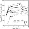 |
Fig. 26 Three different expansion velocities of a PN: VHWHM of the spatially integrated [O iii] 5007 Å line profile, the post-shock velocity, Vpost, behind the outer shock at Rout, and the shock velocity, Ṙout, itself. Shown is the complete time evolution of these velocities for three sequences with the 0.625 M⊙ central-star model and different metallicities (see figure legend). The filled circles mark the snapshots shown in Fig. 24, which correspond also to the moment of maximum [O iii] emission. The relevant model parameters are listed in Table 3 where also the values of VHWHM, Vpost, and Ṙout for the 3 ZGD sequence, not plotted for clarity, are given. The bumps at age ≃1000 years are due to the optically thick/thin transition. |
The complete velocity evolution of three 0.625 M⊙ sequences is rendered in Fig. 26. Plotted are three velocities, Ṙout, Vpost, and VHWHM as a function of the post-AGB age. We see that in general the difference between the measurable VHWHM and the real expansion speed, Ṙout, is quite large: about a factor of two during the [O iii] bright phase of evolution (e.g., filled circles in the figure). During the early, optically thick stage, the velocities increase rapidly with time in all cases. The VHWHM velocities start at very low values, well below the AGB wind velocity of 15 km s-1, because early in the PN evolution when the central star is not very hot, O2+ is restricted to the inner, slowly expanding matter in or around the rim only (cf. Fig. 24, top panels).
As we have already seen for the α = 3 sequences, VHWHM is quite insensitive to the metal content for the whole evolution, in comparison to the shock speed Ṙout (cf. Fig. 13). However, the post-shock gas velocity, Vpost reflects the metal dependence of the shock speed quite well (Fig. 26), but it requires accurate measurements of the faint wings of the integrated line profile, as discussed above.
The velocity bumps (Vpost and Ṙout only) seen close to t ≃ 1000 yr indicate that at this time the models become optically thin for Lyman continuum photons and enter the “champagne” phase of expansion during which the shock speed depends only on electron temperature (sound speed) and radial density gradient (see Paper II). This transition is not seen in VHWHM because the outer nebular region behind the shock contains only little O2+ at this time. Later, at t ≃ 1200 yr, also the outer nebular regions start to contribute significantly to [O iii] line profiles, and the velocity increase flattens out. The deceleration of the shock speed, Ṙout, at higher ages, t > 3000 yr, is due to recombination behind the shock, leading there to much lower electron temperatures and hence lower pressure.
Of course, the maximum amount of [O iii] emission decreases with the oxygen content (see Table 3). This table also shows that this maximum emission value occurs the earlier (i.e. at lower stellar temperatures) the lower the oxygen abundance is (cf. filled circles in Fig. 26). The reason for this behaviour is twofold: (i) the O+ ionising continuum becomes optically thin earlier for lower abundances; and (ii) the number of photons ionising O+ (λ < 353 Å) decreases rapidly with Teff8.
We note also that the expansion speeds do not reach the very high levels of the models shown in Figs. 12 and 13. It has nothing to do with the different central-star masses (0.625 vs. 0.595 M⊙). Rather it is caused by the different density profiles of the circumstellar matter. We recall that the nebular models shown in the Figs. 12 and 13 have initial models with power-law density profiles, ρ(r) ∝ r−α, with α = 3, while the sequences discussed in this section have α = 2, which is the signature of an AGB wind with fixed speed and mass-loss rate. For α = 2, the shock speed relative to the upstream flow is considerably lower than for the α = 3 case (see Fig. 7 in Paper II). The modest shock acceleration during the (optically thin) “champagne” phase seen in Fig. 26 is due (i) to the rise of the electron temperature as the star becomes hotter; and (ii) to the weak acceleration of the AGB wind (=upstream flow) after the passage of the ionisation front.
3.2.2. The [O iii] brightness
The [O iii] emissivity should depend directly on the oxygen content itself. Jacoby (1989) showed, however, that the 5007 Å luminosity changes with roughly the square root of the abundance only. This more modest dependence is explained by two effects which compensate each other partly: the lower oxygen abundance leads to a higher electron temperature, which in turn enhances the emission of collisionally excited lines. Based on optically thick photoionisation models, Dopita et al. (1992) found that there exists a maximum efficiency of converting stellar radiation into [O iii] 5007 Å line emission at about twice the solar oxygen abundance9.
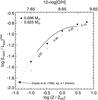 |
Fig. 27 The maximum efficiency of converting stellar radiation into [O iii] 5007 Å line radiation, (L5007/Lstar)max, of 0.696 M⊙ (filled circles) and 0.625 M⊙ models (diamonds) against their metallicity, Z/ZGD. The upper abscissa gives the corresponding oxygen content relative to hydrogen, ϵ(O) (= log (O/H) + 12). The numbers along the dotted line segments connecting the 0.696 M⊙ data points indicate the slope. The inverted parabola (dashed and thick line) is a fit to the predictions of (optically thick) photoionisation models computed by Dopita et al. (1992, Eq. (4.1) therein). The thick portion corresponds to the metallicity range covered by the Dopita et al. models. |
Since our α = 2 sequences (0.696 M⊙ and 0.625 M⊙) cover the range about the bright 5007 Å cut-off of the PNLF, we used them also to check the variation of the 5007 Å luminosity with metallicity Z10. For this purpose we show in Fig. 27 how the maximum 5007 Å luminosity, relative to the bolometric luminosity of the central star (i.e. the efficiency of converting stellar UV radiation into [O iii] 5007 Å line emission), varies with Z, and compare the outcome of our hydrodynamical models with predictions of (optically thick) photoionisation models of Dopita et al. (1992). We used their Eq. (4.1) which is a fit to their model predictions, corrected for the fact that Dopita et al. used a higher solar oxygen abundance (8.84 on the usual scale).
The maximum efficiency of converting stellar radiation into [O iii] 5007 Å line emission is 0.11 for the (optically thick) 0.696 M⊙ models with the Galactic disk composition used here (i.e. ϵ(O) = 8.65). The corresponding stellar effective temperature is about 110 000 K. The maximum efficiency decreases with Z and occurs at progressively lower stellar temperatures, i.e. Teff ≃ 136000 K for Z = 3 ZGD, Teff ≃ 101000 K for ZGD/3 and ≃95000 K for ZGD/10. Our models confirm that this efficiency decrease is weaker than expected because the reduced oxygen abundance is partly compensated for by an increase of the mean electron temperature: from ⟨ Te ⟩ = 8170 K (6 ZGD) over 9500 K (3 ZGD), 11 440 K (ZGD), and 13 980 K (ZGD/3) to 16 650 K (ZGD/10). According to our models, the general Z0.5 dependence of the 5007 Å conversion efficiency quoted in the literature is inaccurate: it holds only for PNe with a metal content around ZGD/3 (see Fig. 27)11.
Our models are, however, partly discrepant to the results of Dopita et al. (1992): for metal contents below the solar one the agreement between our hydrodynamic models and the Dopita et al. fit is reasonably good, but according to their Eq. (4.1) the 5007 Å conversion efficiency reaches a maximum at Z ≃ 3 ZGD not found with our models (cf. Fig. 27). Our models are rather suggesting a levelling off at extremely high oxygen abundances instead. We do not know the reason for this discrepancy, since our hydrodynamic models, being still quite dense and optically thick, are also in ionisation and thermal equilibrium. However, our hydrodynamical sequences mimic consistently the evolution of bright nebulae systems as realistic as possible, whereas the parameter space of the Dopita et al. models is limited and does not cover the high stellar luminosities necessary for PNe close to the luminosity function cut-off. Therefore, we caution that Dopita et al.’s fit formula for estimating the metallicity dependence of the [O iii] cut-off brightness might lead to erroneous conclusions if it is extrapolated into the metal-rich domain (cf., e.g., Ciardullo et al. 2002, Fig. 5 therein).
The models around the 0.625 M⊙ star become optically thin and therefore have always lower conversion efficiencies. A more detailed description how the [O iii] brightness depends on model parameters and/or evolutionary stages can be found in Paper IV, although only for the Galactic disk chemical composition.
4. PNe in distant stellar systems
We have already shown at different occasions, viz. Paper II, Paper III, Steffen & Schönberner (2006), and recently in Paper IV, that the basic physical model used in our simulation of the planetary nebula evolution is very successful in explaining basic observed structures of PNe. A further important test of the quality of our hydrodynamical models is to answer the question if and how well the models are also able to explain global properties of PNe samples in stellar systems so distant that a PN cannot be spatially resolved. Very useful for testing are basic diagrams as those involving characteristic line ratios and expansion velocities measured from the Doppler width of bright emission lines.
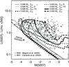 |
Fig. 28 Observed line ratios L(5007)/L(Hα + [N ii]) for PNe of the bulge of M 31 (Ciardullo et al. 2002) and the disk of M 33 (Magrini et al. 2000), as a function of M(5007), compared with the predictions of various hydrodynamical sequences with different metallicities. Evolution proceeds always from faint magnitudes and low line ratios up to maximum 5007 Å emission and then back again, but at higher line ratios. Foreground extinction is considered for the data, but not internal extinction. The arrow indicates the direction of shifts to be applied to the tracks if additional internal extinction occurs. |
4.1. Line-ratio diagrams
We begin with a diagram which combines the line ratio L(5007)/L(Hα + [N ii]) with the brightness in [O iii], M(5007). As an example, Fig. 28 compares the data of two Local Group galaxies, M 31 (Ciardullo et al. 2002) and M 33 (Magrini et al. 2000), with our model predictions. The observations occupy a wedge-like region in this diagram and are, according to Herrmann et al. (2008), roughly bounded from below by a line ![Mathematical equation: \begin{eqnarray*} \log\, \{L(5007)/L({\rm H}\alpha + [\ion{N}{ii}])\}= - 0.37\, M(5007) - 1.16, \end{eqnarray*}](/articles/aa/full_html/2010/15/aa13427-09/aa13427-09-eq245.png) and from above by a horizontal line at
and from above by a horizontal line at ![Mathematical equation: \begin{eqnarray*} L(5007)/L({\rm H}\alpha + [\ion{N}{ii}]) \simeq 4. \end{eqnarray*}](/articles/aa/full_html/2010/15/aa13427-09/aa13427-09-eq246.png) The lower boundary is nearly perfectly matched by all of our models during their early, optically-thick evolution towards maximum 5007 Å emission, virtually independently of their parameters and chemical composition. This boundary is not very well populated because this optically-thick phase of evolution is rather short (cf. Paper IV, Fig. 15 therein). The maximum reachable brightness in M(5007) depends, of course, on the central star mass, the metallicity, and the thick/thin transition. Models which remain optically thick (i.e. the ones with the 0.696 M⊙ central stars) evolve then backwards a little bit above this lower boundary. Models which become optically thin turn then further upwards until L(5007)/L(Hα + [Nii]) ≃ 4 is reached and stay there until the central star fades: the line ratio decrease after the “kink” is the result of the rapid luminosity drop of the central star as hydrogen burning ceases, with a corresponding increase of the [N ii] lines because of a temporary recombination to N+. A slow increase of this line ratio occurs only at fainter magnitudes (M(5007) ≳ 0) because of re-ionisation during the very slow early white-dwarf phase. Because of the fast model evolution between the “kink” and the re-ionisation stage, it is very unlikely that observed objects are in this particular phase.
The lower boundary is nearly perfectly matched by all of our models during their early, optically-thick evolution towards maximum 5007 Å emission, virtually independently of their parameters and chemical composition. This boundary is not very well populated because this optically-thick phase of evolution is rather short (cf. Paper IV, Fig. 15 therein). The maximum reachable brightness in M(5007) depends, of course, on the central star mass, the metallicity, and the thick/thin transition. Models which remain optically thick (i.e. the ones with the 0.696 M⊙ central stars) evolve then backwards a little bit above this lower boundary. Models which become optically thin turn then further upwards until L(5007)/L(Hα + [Nii]) ≃ 4 is reached and stay there until the central star fades: the line ratio decrease after the “kink” is the result of the rapid luminosity drop of the central star as hydrogen burning ceases, with a corresponding increase of the [N ii] lines because of a temporary recombination to N+. A slow increase of this line ratio occurs only at fainter magnitudes (M(5007) ≳ 0) because of re-ionisation during the very slow early white-dwarf phase. Because of the fast model evolution between the “kink” and the re-ionisation stage, it is very unlikely that observed objects are in this particular phase.
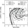 |
Fig. 29 The same data and theoretical sequences as presented in Fig. 28, but now plotted over M(Hα + [N ii]). Objects and sequences are only plotted down to M(5007) = 1, the brightness limit of the samples (cf. Fig. 28). |
We can therefore state that the wedge-shaped region of Fig. 28 is populated by PNe which are evolving along the horizontal part of the HR diagram through maximum [O iii] brightness until the central star begins to fade. Nebulae around the most massive central stars, ≳ 0.63 M⊙, stay always rather close to the lower boundary because they remain optically thick or become only modestly optically thin. Optically thin (or partly thin) models around central stars of ≃0.63 M⊙ to well below 0.59 M⊙ which are on their evolution across the HR diagram fill the entire region between the lower and upper boundary and towards the right until faint magnitudes.
A similar diagram can be made for 5007/(Hα + [N ii) vs. M(Hα + [N ii]) and is shown in Fig. 29. In this diagram the PNe remain bright in (Hα + [N ii]) during the fading of the central stars towards white-dwarf configurations because of recombination and a temporary dominance of the [N ii] lines: the models are now in Hα + [N ii] brighter than in [O iii] 5007 Å by up to 1.5 mag. Hence, our hydrodynamical models suggest that the deficit of objects in the lower right corner of this diagram is not due to sample incompleteness (as proposed by Ciardullo 2010) but is rather a consequence of central star evolution: the early white-dwarf phase where the nebula re-ionises limits the observability of PNe in distant systems if observed in Hα + [N ii].
Another useful diagram for a comparison between data and the predictions of our simulations is that presented in Richer (2006, Fig. 1. It combines the nebular ionsation structure, as measured by [O iii] λ5007 Å and [O ii] λ3727 Å, with the strength of He ii λ4686 Å, which is essentially an indicator of the stellar surface (effective) temperature. An adaptation of Richer’s Fig. 1 is shown in Fig. 30, with the predictions of our evolutionary models included. This diagram is nearly independent of metallicity, as is demonstrated by the three 0.625 M⊙ sequences with different Z, but contains only objects with rather hot and thus evolved central stars because λ4686 Å must be measurable.
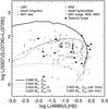 |
Fig. 30 The ratios L(5007)/ [L(3726) + L(3729)] are shown against L(4686)/L(Hβ). The predictions from a selection of our simulations (the two 0.605 M⊙ sequences are from Paper IV) is compared with Local Group data taken from Richer (2006, references therein and priv. comm.). The Galactic bulge data are from Stasińska et al. (1998). Shown are only objects with well-determined line strengths and which are not fainter than two magnitudes below the [O iii] PNLF cut-off. Evolution proceeds from left to right and then down because of recombination. In order to be consistent with the data, the tracks are truncated at two magnitudes below the PNLF cut-off. The kinks seen in two sequences are due to the optically thick/thin transition. |
The interpretation of this diagram, based on our evolutionary models, is as follows:
-
the right border, at L(4686)/L(Hβ) ≃ 1.0, is occupied by highly ionisedobjects for which the emitting volumes of Hβ andHe ii λ4686 Å areabout equal. When recombination occurs, this ra-tio becomes smaller, as is seen in ourmodels. At the same time, the strengthof the [O ii] doubletincreases considerably, more than the λ5007[en-tity!#xa0!]Å line, because themodels become optically thick. These objects close to theright border have very hot and still luminous central stars,producing high nebular excitation, but at the same time alsostrong [O ii] emission,and [N ii] emissionas well;
-
the upper limit L(5007)/ [L(3726) + L(3729)] ≃ 100 is explained either from above by optical thick sequences with massive central stars (≈0.65 M⊙), or from below by sequences with less massive central stars whose models become optically thin during the course of evolution. Objects with massive central stars with ≳ 0.65 M⊙ are obviously not existent (cf. also Fig. 28);
-
a lower boundary for L(5007)/ [L(3726) + L(3729)] is provided by optically thick models around central stars of about 0.6 M⊙ (the three outliers neglected).
The whole observed sample can be interpreted to consist of objects with rather highly ionised/excited optically thick or thin nebular envelopes, as dependent on their evolutionary stage, with central stars with masses between about 0.6 and 0.65 M⊙.
4.2. Expansion properties
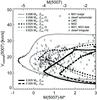 |
Fig. 31 Evolution of PN models in the VHWHM−M(5007) plane. Shown are nebular sequences around central star models of 0.696 and 0.625 M⊙, each of which started with the same initial model but with three different metal contents, as indicated in the figure legend. These sequences are supplemented by ones with less massive central stars of 0.605 and 0.595 M⊙, both with hydrodynamically computed initial envelopes (cf. Table 2). The abscissa gives either the [O iii] magnitude M(5007) as defined by Jacoby (1989) (top) or M(5007)−M ⋆ , with M ⋆ = −4.48 (bottom). The evolution proceeds from low velocities and faint magnitudes over medium velocities and bright magnitudes towards high velocities and again faint magnitudes. The models are compared with a large data set of bright PNe belonging to a variety of galaxies (or parts of them) as indicated in the legend and extracted from Richer (2006, Fig. 4. |
In distant stellar systems one cannot spatially resolve the profiles of emission lines, and information on expansion properties can only be gained from measuring the halfwidth of the profile. Although relevant studies are rare, the following picture emerged: Dopita et al. (1985, 1988) showed for a large sample of Magellanic Cloud objects that there exists an evolution of nebular expansion rates, in terms of line widths, from low to higher values with nebular excitation class or stellar effective temperature. Richer (2006, 2007) reported, based on an extensive spectroscopic study of PNe in the Local Group galaxies, that there is virtually no dependence of the mean expansion properties, as measured from the halfwidth of the 5007 Å [O iii] line, VHWHM(5007), on the metallicity of the parent stellar population. This halfwidth varies between about 8 and 30 km s-1, with a clear accumulation around 18 km s-1 for the brightest objects (Richer 2006, 2007). For the Galactic bulge PNe, Gesicki & Zijlstra (2000) found also a mean VHWHM(5007) of 18 km s-1.
This obvious observed invariance of PNe emission line widths with metallicity seems to contradict strongly the prediction of our hydrodynamical models that expansion speeds generally increase with decreasing metal content. We thus used the sequences discussed in the previous sections for clarifying the situation and interpreting existing observations.
We start with showing the evolution of our models in the VHWHM−M(5007) plane in Fig. 31 which is adapted from Fig. 4 in Richer (2006) and contains also the same data from different galaxies and/or parts of them. All the relevant data are now also available from Richer et al. (2010b). The theoretical tracks of our two most massive central stars (0.696 and 0.625 M⊙) surrounded with PNe models with different metallicities (Z = ZGD, ZGD/3, ZGD/10) suggest that such a diagram is not well suited to study and compare expansion properties of bright PNe in different environments since all tracks cover or embrace the observational data with no obvious trend with metal content. Moreover, at their maximum M(5007) brightness, all models, independently of their metallicity (cf. Fig. 26), provide practically the same halfwidth velocity of VHWHM ≃ 18 km s-1, in astonishingly good agreement with the observations!
The theoretically expected distribution of the HWHM velocities depends on the evolutionary speed through the VHWHM−M(5007) plane and the central-star mass distribution. In order to illustrate the former better, we show in Figs. 32 and 33 histograms which give the visibility time Δt spent by a particular model within a velocity bin of ΔVHWHM = 1 km s-1. Thus, Δt is a proxy for the expected number of PNe per velocity interval of 1 km s-1. These histograms combine the information contained in Figs. 26 and 31.
In particular, Fig. 32 displays the results for the 0.625 M⊙ sequences. The total simulation time shown in these figures is much longer than seen in Fig. 31, and the tracks extend thus to fainter magnitudes. The VHWHM bins are additionally broken down into magnitude intervals to account for the fact that the velocity is not a monotonic function of M(5007) (Fig. 31). For instance, the low-velocity stage is passed rather quickly, which may explain the paucity of low-velocity objects seen in Fig. 31.
We show, for comparison, also the Ṙout distributions. They appear bimodal where higher velocities belong to the high-luminosity phase as the central star crosses the HR diagram, and lower velocities to the recombination stage as the stellar luminosity fades.
The histograms seen in Fig. 33 belong to three simulations with the 0.696 M⊙ central-star model. Although the time scales are shorter, the general behaviour is the same as already discussed above. The histograms shown in Figs. 32 and 33 demonstrate clearly that in a magnitude limited sample in which only the brightest PNe are contained all VHWHM are quite low and cluster around 20 km s-1. Very low halfwidth velocities (< 10 km s-1) occur only for faint models at the beginning of their brightness evolution (cf. Fig. 26). Considering only models within the brightest bin of each sequence, the means of their halfwidth velocities are between 18 and 20 km s-1, i.e. virtually independent of their metal content.
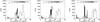 |
Fig. 32 Times Δt spent by the models within the velocity intervals ΔVHWHM = 1 km s-1 and |

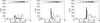 |
Fig. 33 The same as in Fig. 32 but for the three 0.696 M⊙ sequences with Z = ZGD (left), Z = ZGD/3 (middle), and Z = ZGD/10 (right) whose brightness evolution is also seen in Fig. 31. The maximum post-AGB age considered is 1200 years. The Δt for the faintest magnitudes are lower limits only because of this time limit. |
From the discussion of the Figs. 31−33 we see that our models are in excellent agreement with measurements of bright PNe in distant stellar systems. The VHWHM distribution of bright Galactic bulge PNe peaks between 15 and 20 km s-1 (Gesicki & Zijlstra 2000, Fig. 6 therein), and the 11 bright Virgo cluster PNe with spectroscopically resolved [O iii] 5007 Å lines have VHWHM between 12 and 22 km s-1, with a mean value of 16.5 km s-1 (Arnaboldi et al. 2008). The bright PNe of the Local Group of galaxies plotted in Fig. 4 of Richer (2006) cluster in the brightness range of M(5007) ≃ −4.2...−3.5, and their eye-estimated mean VHWHM is ≃18 km s-1. Richer et al. (2010b) argued again that the mean 5007 Å line width is not dependent upon maximum [O iii] luminosity, metallicity or age of the progenitor population. All these findings are well explained by our hydrodynamical models, especially by the 0.625 M⊙ sequences (Fig. 31).
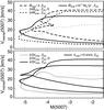 |
Fig. 34 VHWHM(5007) vs. M(5007) for 0.696 M⊙ sequences (α = 2) with the AGB mass-loss rates (top) and AGB wind velocities (bottom) varied, as indicated in the legends. In the top panel Vagb = 15 km s-1 holds in all cases, whereas we have always Ṁagb = 1 × 10⁻⁴ M⊙ yr-1 in the bottom panel. Our standard 0.696 M⊙ sequence with Ṁagb = 1 × 10⁻⁴ M⊙ yr-1 and Vagb = 15 km s-1 serves in both panels as a reference (solid lines). Evolution proceeds always from low to high velocities. |
All sequences discussed so far have the same initial model, viz. they start with an assumed constant AGB mass-loss rate of 1 × 10⁻⁴ M⊙ yr-1 and a constant outflow velocity of 15 km s-1. Here we briefly investigate how the above findings depend on initial mass-loss rate and wind velocity. For this purpose we computed additional sequences for the 0.696 M⊙ post-AGB stellar model (α = 2): the initial mass-loss rate of 1 × 10⁻⁴ M⊙ yr-1 was doubled/halved and the initial wind velocity of 15 km s-1 lowered/increased by 5 km s-1. The results are shown in Fig. 34.
The interpretation of the influence of the AGB wind velocity is simple: the initial velocity enters as a corresponding up and downshift of VHWHM(5007), rather independently of the metal content (Fig. 34, bottom, sequences 2/3Vagb with ZGD and ZGD/3, and 4/3Vagb, ZGD). AGB mass-loss rate differences have a more subtle impact. The increased Ṁagb leads to a corresponding lower value of VHWHM(5007) at the luminosity maximum, as expected. A lower Ṁagb, however, does not change the expansion much at maximum brightness (Fig. 34, top). The reason is that, because of the less dense AGB wind, the nebular shell becomes, in this particular case, optically thin well before its maximum possible [O iii] line luminosity is reached. The [O iii] brightness becomes temporarily lower until the shell recombines and becomes again optically thick, and hence brighter. Concerning the expansion behaviour at maximum brightness, we see also that the metal content is virtually of no influence (Fig. 34, top, sequences 2Ṁagb, ZGD and 2Ṁagb, ZGD/3).
For completeness we add the discussion of two sequences with initial envelopes generated by radiation-hydrodynamics simulation along the upper AGB (sequences Nos. 6 and 6a of Paper IV). Both sequences have normal metallicities, i.e. Z = ZGD, and their VHWHM evolution with M(5007) has already been displayed in Fig. 31. The corresponding histograms are seen in Fig. 35.
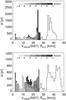 |
Fig. 35 Same as in Fig. 32 but for the sequences with 0.605 M⊙ (top) and 0.595 M⊙ (bottom) already presented in Fig. 31. The post-AGB age ranges considered are 12 000 years for both sequences. |
The behaviour of these sequences is somewhat different: at VHWHM(5007) ≃ 10...11 km s-1 the models become optically thin and reach then also their maximum [O iii] brightness. The HWHM velocity further increases steadily during the optically thin part of evolution until recombination begins. The total range of VHWHM(5007) within the brightest 3 mag is for both sequences ≃4 to ≃25 km s-1. On average, the real expansion, as determined by Ṙout, is again considerably higher, viz. nearly a factor of two (Fig. 35).
Since the [O iii] brightness depends on the nebular metal (oxygen) content, it might be more useful to plot VHWHM(5007) against the Hβ brightness in order to get rid of metallicity effects in both the observation and theory. We expect that in a VHWHM−M(Hβ) plane the tracks of models which differ only in their metal content will be very similar, at least during the early evolution. Figure 36 confirms our conjecture: there is a rather tight correlation between M(Hβ) and VHWHM, and at maximum Hβ brightness (M(Hβ) ≃ −2) the HWHM velocities are ≃16 ± 2 km s-1 for 5007 Å and ≃20 ± 2 for Hβ. Larger differences between the tracks occur during later phases when recombination determines the ionisation structure of our nebular models for ages above 3500 years (cf. Fig. 26).
The moderate variation of VHWHM(Hβ) is easily explained: the hydrogen line emerges from the entire ionised region, and its line width is controlled by the fast moving gas behind the outer shock (cf. Fig. 24, top panels) together with the (comparatively) high thermal broadening (≈10 km s-1). In the beginning, thermal broadening dominates, but later expansion broadening becomes more important. Thermal broadening of oxygen lines is four times less, and the velocity evolution of, e.g., [O iii] 5007 Å can reasonably be traced by the line width. Very early, the O2+ zone is restricted to the innermost nebular regions only, close to the contact discontinuity where the gas is nearly stalling. Hence, VHWHM(5007) is very low, much lower than the AGB wind velocity: only 4−5 km s-1 as compared to Vagb = 15 km s-1. Later, VHWHM(5007) steadily increases mainly because the O2+ zone extends until it embraces the whole nebula and approaches finally VHWHM(Hβ).
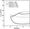 |
Fig. 36 Run of VHWHM(5007) and VHWHM(Hβ) vs. M(Hβ) for the different 0.625 M⊙ sequences. Evolution proceeds in all cases from faint magnitudes and low velocities towards faint magnitudes and higher velocities. |
Our model simulations suggest that large differences between velocities measured from the widths of hydrogen lines and lines of heavier ions are not only the result of different thermal broadening. Rather, these differences also point to the existence of a substantial positive velocity gradient within all PNe. Such velocity gradients, as they are predicted by hydrodynamical simulations, have indeed been found for a few galactic PNe by means of a careful analysis of high-resolution slit spectrograms (cf., e.g., Gesicki et al. 1996, 1998).
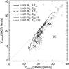 |
Fig. 37 VHWHM(5007) vs. VHWHM(Hβ) for four 0.625 M⊙ and two 0.605 M⊙ sequences with different metallicities as indicated in the legend. Evolution proceeds always from low towards higher velocities. Plotted are only the evolutionary phases with Teff ≤ Tmax. The models are compared with recent HWHM velocity measurements of Milky Way bulge objects, either with apparently unsplit line profiles (filled symbols) or with split profiles (open symbols), provided to us by Richer (see also Richer et al. 2008, 2009, 2010a), and assuming that the halfwidth velocities of Hβ and Hα are the same. Only objects with 5007 Å line strengths greater than Hβ are considered. Accordingly, thin line sections at low velocities indicate models for which L(5007) ≤ L(Hβ). The model profiles are broadened by a Gaussian with FWHM of 11 km s-1 in order to comply with the spectral resolution of the observations. Crossed symbols mark objects which are known to posses [WC]-type central stars (see Górny et al. 2004). |
Recently, Richer et al. (2009) presented halfwidth velocities of Galactic bulge PNe based on both Hα and [O iii] 5007 Å. These measurements are shown in Fig. 37, together with selected model sequences relevant for bright bulge objects of the Milky Way. One sees that the HWHM velocities predicted by our models are in excellent agreement with measurements of the slowly expanding objects with unsplit lines, which are obviously also the younger ones of this sample (filled symbols). The agreement becomes poorer for a majority of the larger, spatially resolved PNe with split lines (open symbols).
However, for a full appreciation of Fig. 37 we have to consider that all Galactic bulge objects are to some extent spatially resolved. The typical coverage of the slit is between 30% and 50% for the slowly expanding objects (filled circles in Fig. 37) and usually less for the faster expanding PNe with doubly peaked profiles. Going from low to high spatial resolution increases the width of the line profiles of both the [O iii] and Hβ line by very similar amounts: in the low velocity regime we estimated from model calculations typical values of 3 km s-1 for 5007 Å and 4 km s-1 for Hβ. For doubly peaked profiles this shift is larger, and this effect may explain the slight offset to the right that is seen at higher velocities between the observations and our models (open symbols in Fig. 37).
Despite of the small inconsistency between the velocities derived from our (unresolved) theoretical line profiles and those measured by Richer et al. (2009, 2010a), the interpretation of Fig. 37 is not really affected: we see how the ionisation stratification develops with time (or velocity) in nebular structures with positive velocity gradients in the same way as appropriate hydrodynamical models predict. Note also that the two metal-poor sequences (ZGD/3, ZGD/10) do not predict the correct relation between hydrogen and oxygen line widths and are too faint in 5007 Å at low velocities.
Spectroscopy done by Górny et al. (2004) revealed that the sample of bulge PNe used by Richer et al. (2009, 2010a) contains several objects with WC central stars, which are marked in Fig. 37 by crossed symbols. Remarkably, their velocity behaviour appears to be the same as that of their “normal” counterparts (apart from the outlier). Of course, the number of WC-type objects in this Richer sample is too small in order to allow a more definitive statement.
Richer’s linewidths measurements of PNe of the Galactic bulge are finally plotted in Fig. 38 over the Hβ absolute brightnesses, assuming a distance to the bulge of 7.5 kpc and selecting only the younger objects with unsplit lines. There is again close agreement with the predictions of our model sequences. Central stars of about 0.6 M⊙ appear to be sufficient to explain the observed maximum Hβ brightness achieved by the PN population of the Galactic bulge.
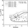 |
Fig. 38 Similar as in Fig. 36 but now for VHWHM(5007) and VHWHM(Hβ) vs. M(Hβ) predicted from model sequences with different central stars and the same metallicity. Evolution proceeds again from faint magnitudes and low velocities towards faint magnitudes and higher velocities. These theoretical predictions are again compared with the Galactic bulge sample of Richer et al. (2009, 2010a) already used in Fig. 37. Plotted are only objects with unsplit lines, and thus the region containing higher velocities at low brightness is devoid of objects. Each object (except for a few cases) is plotted twice, with its VHWHM(5007) (filled symbols) and VHWHM(Hβ) (= VHWHM(Hα)) (open symbols). We assumed a distance of 7.5 kpc for all objects. The theoretical profiles are broadened by a Gaussian with FWHM of 11 km s-1 in order to resemble the observations. |
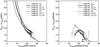 |
Fig. 39 Ṙout/VHWHM vs. VHWHM for [O iii] 5007 Å (left) and Hβ (right) and for the different types of hydrodynamical sequences. The evolution proceeds from low to high line widths, or VHWHM. |
We can summarise the results of this section as follows:
-
Measuring the expansion of bright extragalactic PNe bymeans of the HWHM method, the only pos-sible one for distant objects which cannot be spatially re-solved, is not very fruitful for more detailedstudies. Although there exists an evolution of VHWHM with time in,e.g. [O iii] lines,the dependence on metallicity is extremelysmall and can virtually be neglected. The time evolutionof VHWHM does by no means reflect the real expan-sion (cf. also Fig. 26). TypicalHWHM velocities at maximum nebularbrightness are ≲ 20 km s-1,for all metallicities considered here. Lowerspeeds seen during the early PN evolution areentirely due to ionisation stratification in conjunction witha positive radial velocity gradient. However, the real expan-sion speed depends on metallicity and can be larger by fac-tors of two or more (Figs. 26, 32,and 33; see also the next section).
-
Based on our hydrodynamical simulations reported here we state further that the very narrow range of halfwidth velocities (VHWHM) measured for the brightest PNe of galaxies with quite different properties as reported by Richer (2007, Fig. 1 leads to only one conclusion: stellar evolution at the tip of the AGB occurs independently of the properties of the underlying stellar population. The close agreement of observations with our model predictions implies that the initial condition chosen by us at the tip of the AGB for, e.g., a 0.625 M⊙ stellar remnant, viz.
M⊙ yr-1 with Vagb = 15 km s-1, are very close to reality. -
The narrow range of observed halfwidth velocities indicates further that everywhere the same main process for formation, shaping, and evolution of PNe is at work: heating of sufficiently dense circumstellar wind envelopes by photoionisation, setting up an expanding shock wave which defines the outer edge of the PN. Wind interaction and/or magnetic fields, although important in single cases and/or during certain phases, is obviously not the main shaping agent, contrary to common wisdom.
4.3. The real expansion
Our simulations demonstrate clearly that it is impossible to derive the real expansion properties of PNe from a simple measurement of the halfwidths of spatially unresolved line profiles. Because of the ionisation and/or density structures together with projection effects the contribution of the fastest moving matter to (integrated) line profiles is strongly reduced.
However, we can use our hydrodynamic models to quantify the relation between the real expansion, as defined by the propagation of the outer shock, and the spectroscopically measured expansion deduced from the HWHM of an emission line profile, which is in practice that of [O iii] 5007 Å, or also that of Hα or Hβ. Figure 39 illustrates how the ratio between shock speed and VHWHM of [O iii] 5007 Å and Hβ (or Hα) changes during the nebular evolution, as based on our simulations. We see that all types of models behave in the same way: the ratio between both velocities generally decreases with time and comes close to unity during the end of evolution.
The behaviour of Ṙout and VHWHM seen in Fig. 39 can be explained as follows: first of all, we recall that Ṙout is determined by the density gradient of the (fully ionised) ambient medium and the sound speed of the nebular gas behind the shock front (cf. Paper II). VHWHM, however, contains all the globally averaged information of gas motions and the density distribution inside the nebula measurable via the Doppler effect. If the nebula has a stratified ionisation structure, VHWHM depends also on the ion used.
For instance, during the early ionising phase of the PN evolution the ratio between Ṙout and VHWHM is quite large (greater than 3 for VHWHM(5007) ≲ 10 km s-1), since O2+ is restricted only to the strongly decelerated inner regions (cf. Fig. 13, right panel). The situation is different for hydrogen lines (Fig. 39, right panel): since hydrogen ionisation starts while the matter is still moving with the AGB-wind velocity, VHWHM starts with similar values of, e.g., 10−15 km s-1. The ratio of Ṙout and VHWHM does not exceed a factor of about two.
With progressing ionisation, VHWHM(5007) catches up later in the evolution because progressively faster moving matter from the outer regions behind the shock contributes to the integrated line profile. During the recombination phase it may happen that the shock is being decelerated so much that Ṙout may fall even below VHWHM, i.e. Ṙout becomes lower than the flow speed of the nebular gas (cf. Fig. 39, left, the 0.696 M⊙, ZGD models with VHWHM(5007) > 30 km s-1).
We see especially in the left panel of Fig. 39 also that for fixed VHWHM and for the same configurations (central star mass and initial envelope model) the correction for Ṙout increases somewhat if the metallicity decreases. The shock propagation speed is controlled by the electron temperature and makes metal-poor and hotter nebula more dilute in their outer regions. The inner denser regions, however, are less accelerated because of the reduced wind power. Altogether, the width of the integrated line profile does not change to the same extent (full ionisation provided, cf. Fig. 26). Such a metallicity influence on the line width is not seen for hydrogen lines (Fig. 39, right), most likely because of the generally larger thermal contribution to the line broadening.
The interesting phase from an observational point of view occurs when nebulae evolve through their brightest stage (in [O iii]). We have seen above that this happens for VHWHM(5007) ≃ 15...25 km s-1, which implies correction factors of 1.5...2.5 to get the real expansion speeds. A mean correction factor of two appears therefore to be a reasonable choice for the brightest nebulae of a sample. Figure 39 (right panel) suggests that two is also a quite useful mean correction factor for hydrogen lines.
4.4. The case of the Magellanic Cloud PNe
The Magellanic Clouds (MC) contain a rather large population of planetary nebulae which can also be studied down to fainter magnitudes than it is possible in most other extragalactic systems. Thus, the MC sample of PNe is well suited for studying aspects of PN evolution in an extragalactic system.
Dopita et al. (1985, 1988) used in their seminal work of the Magellanic Cloud PNe a somewhat different definition to measure the expansion of a spherical gaseous shell: Vexp = 0.911VFWHM, where VFWHM is twice the HWHM velocity. Assuming a Gaussian shape for the intrinsic profiles, this is equivalent of Vexp being half of the full width at 10% maximum line intensity, VHW%10M, or Vexp = 1.82VHWHM, with VHWHM being the velocity deduced from the HWHM of the line profile. Thus, Dopita et al.’s “expansion” velocities, Vexp, are higher by nearly a factor of two as compared to the more widespread use of VHWHM. The advantage of this definition is, however, that the such measured velocity is much closer to the maximum gas velocity behind the outer shock (see the discussion in Sect. 3.2.1 and Table 3).
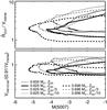 |
Fig. 40 Evolution of Ṙout/VHWHM (top) and VHW10%M/0.911VFWHM (bottom) vs. absolute 5007 Å brightness, M(5007), for different nebular model sequences. In both panels, evolution proceeds from faint magnitudes at the upper right towards faint magnitudes at the lower right. |
Dopita et al. (1985, 1988) did not measure VHW%10M directly, but used Vexp = 1.82VHWHM instead, thereby implying implicitly a Gaussian shape for the intrinsic line profile. In reality, however, the spatially integrated line profiles are by no means Gauss functions (cf. Fig. 24, bottom panels). A moderate broadening by finite spectral resolution does not change this. Additionally, the shape of the line profile changes with time because the density distribution and the velocity field develop as the model traverses the Hertzsprung-Russell diagram.
The whole situation is illustrated in Fig. 40 where the relations between Ṙout and VHWHM (top panel) and between VHW10%M and 0.911VFWHM (bottom panel) are displayed as a function of the nebular brightness for the different hydrodynamical PN sequences used here. VHW10%M expresses the velocity derived from the 10% level of the line profile. For a Gaussian we expect VHW10%M/0.911VFWHM = 1 (see above). From Fig. 40 (bottom panel) we see that the line profiles deviate considerably from a Gaussian shape, mainly during the late evolution when the models become more extended.
The top panel of Fig. 40 is equivalent to Fig. 39 but shows more clearly how the correction factor, to be applied to VHWHM, depends on the nebular brightness. One sees again that a factor of two is quite reasonable for most models while evolving through their brightest stage. One sees also more clearly that only for the metal-rich model sequence around 0.696 M⊙ this factor falls below unity along the fading branch of evolution, as seen already above (Sect. 4.3).
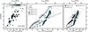 |
Fig. 41 Nebular excitations, E, vs. 5007 Å velocities, Vexp = 0.911VFWHM, for Magellanic Clouds PNe (Dopita et al. 1985, 1988) and our hydrodynamical simulations. Observed objects and models are broken down into the same M(5007) brightness classes, as indicated by the symbol sizes: the larger the symbol, the brighter the object or model, respectively. The approximate brightness range covers 4 mag. The top abscissa is labelled in terms of VHWHM for easier comparison with previous figures. Left panel: LMC and SMC PNe additionally broken down into classes of different oxygen abundances (from Dopita & Meatheringham 1991a,b), visualised by various grey shades. The darkest grey corresponds to ≥ ZGD/2, the lightest grey to ≤ ZGD/5. The vertical arrow indicates the oxygen abundance corresponding to ZGD/3. Middle panel: comparison of observations with the model sequences as indicated. The gaps seen in the model sequences are artefacts due to the definition of E combined with the lower oxygen abundance of the Clouds (Eqs. (5), see text there). Note that the spacings of the models within a sequence does by no means reflect the speed of evolution. Right panel: a 0.625 M⊙ model sequence (α = 2, Z = ZGD/3) with different initial parameters, Ṁagb = 0.5 × 10⁻⁴ M⊙ yr-1 and Vagb = 7.5 km s-1 (filled triangles), compared with the 0.625 M⊙ZGD/3 sequence from the middle panel and a metal richer (Z = ZGD) 0.625 M⊙ sequence (see legend). |
4.4.1. Nebular excitation and expansion
From the rather large samples of LMC and SMC PNe Dopita et al. (1985) and Dopita et al. (1988) found a positive correlation of Vexp with the nebular excitation parameter E, defined as ![Mathematical equation: \begin{displaymath} E = 0.45\,\left[X(5007)/X({\rm H}\beta)\right], \ \ \ \hspace{1.8cm} 0.0<E<5.0, \end{displaymath}](/articles/aa/full_html/2010/15/aa13427-09/aa13427-09-eq314.png)
![Mathematical equation: \begin{equation} E = 5.54\,\left[X(4686)/X({\rm H}\beta) + 0.78\right], \ \hspace{1.0cm} 5.0\le E < 12.0, \label{exc} \end{equation}](/articles/aa/full_html/2010/15/aa13427-09/aa13427-09-eq315.png) (5)where X stands for line luminosities or fluxes, respectively (Dopita et al. 1992). This correlation must be interpreted as the evolution of the nebular expansion speed with time or stellar effective temperature.
(5)where X stands for line luminosities or fluxes, respectively (Dopita et al. 1992). This correlation must be interpreted as the evolution of the nebular expansion speed with time or stellar effective temperature.
Equations (5) constitute a purely empirical definition of the nebular excitation state in close resemblance to the original Morgan (1984) classification scheme (cf. Dopita & Meatheringham 1990). Although the low excitation branch, E < 5, depends directly on the oxygen abundance, Eqs. (5) are quite useful as a proxy for the nebular evolution. However, E is, like the brightness, neither a unique function of time nor of stellar temperature (see, e.g., Fig. 15 in Paper IV).
To perform a new interpretation by means of our hydrodynamic sequences, we proceeded as follows: firstly, we computed the excitation parameters E of LMC and SMC PNe from the line fluxes available in the literature by means of Eq. (5) and used Vexp as determined by Dopita et al. (1985) and Dopita et al. (1988). We discarded objects whose line profiles could only be fitted by a double Gaussian since they have most likely an extreme bipolar shape not suitable for comparison with spherical models. We did then the same with our nebular models, i.e. we derived E from the model’s line strengths and determined Vexp from the line profiles according to the Dopita et al. prescription given above and applying an appropriate broadening (Gaussian with a FWHM of 10 km s-1) to simulate instrumental broadening.
The result is shown in Fig. 41 which provides not only velocity and brightness information of Dopita et al. (1985, 1988), but also oxygen abundances determined by photoionisation modelling of Dopita & Meatheringham (1991a,b). The left panel of Fig. 41 displays the Magellanic Clouds objects, broken down into classes of different M(5007) brightnesses and oxygen abundances (relative to hydrogen), as indicated by the symbol sizes and their grey values. This panel is a new version of Fig. 4 in Dopita et al. (1988) with more accurate excitation values.
There is a broad positive correlation between excitation class and expansion velocity of the Magellanic Clouds objects in the sense that there are no low velocities for high excitation and no high velocities for very low excitation. The distribution is very narrow at low velocities (Vexp ≲ 15 km s-1), but becomes rather wide at higher velocities or excitations, independently of the oxygen abundance. One notices, however, that the brightest objects have preferentially also the highest amount of oxygen.
The left panel of Fig. 41 shows again what is already evident from our Figs. 31 and 4 in Dopita et al. (1992): the most luminous objects, which accumulate around E ≃ 6 (big symbols in Fig. 41), have rather modest expansion rates (in terms of VHWHM, top abscissa) between 15 and 20 km s-1. The fainter objects have, in general, either low (young objects) or high expansion rates (older objects). Obviously PNe in the Magellanic Clouds show the same expansion behaviour as PNe in the Galactic bulge, the Local Group, and the Virgo cluster.
The middle panel of Fig. 41 compares the observations with the predictions of our hydrodynamical simulations in terms of excitation, brightness, and halfwidth velocities. We used the slightly metal-deficient models with Z = ZGD/3 in order to take the metallicities of both Clouds roughly into account. Note that the excitation E, if computed according to Eqs. (5), does not reach the limit E = 5 from below because of the reduced oxygen content, creating thereby an artificial gap in the presentations of Fig. 41.
For a full appreciation of this figure it is important to realise that the excitation E does not only depend on the stellar temperature but also on the nebular density. Lower densities favour higher excitations for a given stellar temperature. Therefore, the models around the 0.605 M⊙ central star, which are less dense than the models around the 0.696 M⊙ star and become optically thin during the course of evolution, reach higher excitations than the 0.696 M⊙ models In spite of the fact that for the latter the central star achieves much higher temperatures (e.g. 240 000 K instead of only 160 000 K for the 0.605 M⊙ case). We showed in Paper IV (Figs. 13 and 14 therein) that the highest degree of excitation (E ≈ 10) is only reached by optically very thin nebulae. An example is the α = 3, 0.595 M⊙ sequence shown in Fig. 41 (middle): it does not recombine much and reaches the highest expansion rates at the highest possible excitation level, as given by the He/H ratio which is 0.11 for our models.
Figure 41 demonstrates that all objects start their expansion (at E ≃ 0), as the models do, very slowly, with VHWHM(5007) of only a few km s-1. Since our models have AGB-wind flows with 10 or 15 km s-1, these low values are thus no indication for a similarily low AGB-wind velocity. We have already explained above this phenomenon as the consequence of the ionisation stratification (of oxygen) in combination with a steep velocity gradient within the ionised shell during the early evolution of a PN (cf. Fig. 13).
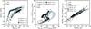 |
Fig. 42 Various correlations for the same objects and model sequences as in Fig. 41. The meaning of the symbols (PNe and models) is the same as in Fig. 41. The triangles refer always to the new 0.625 M⊙ sequence introduced in the right panel of Fig. 41. All sequences are only plotted until maximum stellar temperature is reached, in order to avoid some confusion, and also because they become too faint. Left panel: nebular expansion from the [O iii] 5007 Å line width vs. stellar temperature for Magellanic Cloud PNe compared with the hydrodynamical model sequences. The observed stellar temperatures are from the extensive photoionisation modelling by Dopita & Meatheringham (1991a,b). Middle panel: correlation between velocities derived from [O ii] 3726 Å and [O iii] 5007 Å according to Dopita et al. (1988) and the hydrodynamical models. Right panel: reduced nebular mass vs. radius relations for Magellanic Clouds PNe and our hydrodynamical models. Data again from Dopita & Meatheringham (1991a,b). |
During the course of evolution the line widths increase, with some spread in terms of excitation and VHWHM which is caused by the different combinations of central star and circumstellar envelope. Obviously, Fig. 41 (middle) implies again that for all observed PNe the same mechanism for their formation and expansion must be at work, which, according to our models, is heating by ionisation and the immediate creation of an expanding shell bounded by a shock front.
During recombination, E drops to intermediate values although the star remains very hot (Teff ≳ 120000 K). The ionisation becomes stratified, and the O2+ is confined to the inner regions closer to the hot central star. The outer shock is decelerated because of the post-shock pressure drop due to recombination while the inner region is still accelerated by the thermal pressure of the hot bubble (shocked stellar wind gas) and somewhat later, by reionisation. Because of this, VHWHM may decreases during recombination, but continues later to increase further (cf. 0.605 M⊙ sequence in Fig. 41, middle panel).
From Fig. 41 (middle panel) we see, however, that our model sequences do not match the observations perfectly, which, of course, is of no surprise since the models are not tuned to match objects of the Magellanic Clouds. For the most relevant sequence, 0.625 M⊙ and Z = ZGD/3, E falls behind the VHWHM evolution, while the 0.605 M⊙ sequence has the correct expansion property but remains a little bit too faint at medium excitations. The 0.595 M⊙ sequence stays always far too faint (cf. their small symbols) and is thus omitted for further considerations. The 0.696 M⊙ sequence becomes somewhat too bright, although the VHWHM evolution is marginally right.
We have already seen in Fig. 34 that a variation of the initially chosen AGB-wind velocity leads to a corresponding variation of the PN expansion rate. Hence, we expect that models with different AGB-wind velocities would be shifted horizontally in a diagram such as displayed in Fig. 41. To test this possibility, we used the 0.625 M⊙, Z = ZGD/3 sequence with Ṁagb = 0.5 × 10⁻⁴ M⊙ yr-1 and Vagb = 7.5 km s-1. This combination of mass-loss rate and AGB-wind velocity ensures that the initial circumstellar density profile is the same as in the comparison sequence. However, because of the more slowly moving AGB material, also VHWHM increases now more in pace with E, although objects with the highest excitations are now not covered (Fig. 41, right panel).
For comparison, we replotted here also the 0.625 M⊙ sequence from the middle panel, supplemented by a corresponding metal richer sequence with Z = ZGD. One sees that just changing the metallicity will not lead necessarily to a better match with the observations.
One concludes from this exercise that a mixture of models with somewhat lower final mass-loss rates and lower AGB wind speeds and of models as they are used here would lead to a good match with the observed HWHM velocity-excitation correlation of PNe in the MCs.
4.4.2. Stellar temperature and nebular expansion
Because of the dependence of E on both stellar temperature and (mean) nebular density, it is not surprising that the observed sample cannot be described by a single evolutionary track. A more direct comparison can be made if we correlate Vexp (= 0.991VHWHM) of the nebula with the effective temperature of the central star (cf. Fig. 6 in Dopita & Meatheringham 1991a). We used the same sample shown in Fig. 41 and selected all those objects for which Dopita & Meatheringham (1991a,b) provided stellar temperatures, based on detailed photoionisation models.
The use of the stellar temperature (if accurately known) as a proxy for the time evolution across the Hertzsprung-Russell diagram is useful since (i) it is a distance-independent quantity; and (ii) its range depends weakly on the stellar mass. Furthermore, the two driving forces for the nebulae, the radiation field and the wind, depend directly on the stellar effective temperature.
Figure 42 (left panel) is an adaption of the Dopita & Meatheringham figure mentioned above and demonstrates again that the signatures of nebular expansion, as measured by a suitable line width, evolve with time (or stellar effective temperature), and that this time evolution is correctly described by our hydrodynamical model sequences. Note that the theoretical sequences shown in Fig. 42 cover very different time spans, ranging from about 10 000 years for 0.605 M⊙, through about 4000 years for 0.625 M⊙, to about 1000 years only for 0.696 M⊙. Yet the sequences are nearly “degenerate” if the stellar temperature is used as a proxy for the evolutionary progress across the Hertzsprung-Russell diagram.
A similar correlation between nebular expansion and stellar temperature was also found for Galactic PNe with double shell structures in our Paper II where typical flow speeds of shell and rim gas were measured from spatially resolved high-resolution echelle spectra.
4.4.3. Nebular ionisation stratification and expansion
An indication of the ionisation structure and the velocity field of a PN can be gained by measuring the HWHM velocities of different ions of the same element, viz. of O+ and O2+ (e.g. Dopita et al. 1988, their Fig. 3). These authors found that velocities derived using O+ are in most cases higher than those from O2+. We replotted their data in Fig. 42 (middle), supplemented again by our dynamical models in order to check whether our models are able to predict the same behaviour.
We see from Fig. 42 (middle) that the observed trend of the expansion signatures are, indeed, quite well matched by our models, although the [O iii] velocities of the younger models are somewhat lower than observed. At the beginning of the evolution all models behave similarily, with VHWHM([Oii]) > VHWHM([Oiii]), because of the radial ionisation stratification of oxygen and the positive velocity gradient. Later, if the models are optically thin and O2+ becomes the main ionisation stage throughout the model, both ions, O+ and O2+, trace about the same nebular regions, albeit with different fractions, and hence VHWHM([Oii]) ≃ VHWHM([Oiii]). This transition occurs quite rapidly and produces the left turn of the model tracks seen in Fig. 42 (middle).
Note that the models around the 0.696 M⊙ central star remain optically thick throughout the whole evolution, with VHWHM([Oii]) always greater than VHWHM([Oiii]) until the star begins to fade. This sequence with its quite massive central star model, 0.696 M⊙, is obviously not an option for PNe in the Magellanic Clouds, also because, as we mentioned already above, the models become too bright.
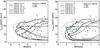 |
Fig. 43 Comparison of HWHM velocities vs. absolute magnitudes of Magellanic Cloud PNe with different model predictions as indicated in the legends. The dashed-triple-dotted line correspond to the Vagb = 7.5 km s-1 sequence. The velocity measurements are again from Dopita et al. (1985, 1988), but here VHWHM is shown, instead of their Vexp, against M(5007) (left) and M(Hβ) (right). The 5007 Å fluxes are from Jacoby et al. (1990). True distance moduli and extinction values c used are 18.37 and 0.28 for the LMC and 18.72 and 0.26 for the SMC (Dopita et al. 1992). |
The interpretation of Fig. 42 (middle) is the following: if VHWHM([Oii] is significantly greater than VHWHM([Oiii]), the object in question is ionisation stratified and optically thick, irrespective of the amount of VHWHM. If both velocities are similar, the object is optically thin, which is the case for most of the MC objects plotted in Fig. 42 (middle). It appears, however, that there exists often a tendency for Vexp([Oii]) of being greater than Vexp([Oiii]) by ≈10 km s-1, on the average. This behaviour is best matched by our 0.605 M⊙ sequence during the optically thin phase.
4.4.4. Evolution of nebular masses
As PNe expand into the AGB matter, their mass must increase with time. This has been convincingly demonstrated by Dopita & Meatheringham (1991a,b) in their study of the Magellanic Cloud PNe. The mass increase with time (or radius) is ruled by the speed of the (outer) shock and the density profile of the former AGB wind matter. A decrease of the ionised mass is possible during the recombination stage as the central star fades.
In the right panel of Fig. 42 we compare the Dopita & Meatheringham (1991a,b) data with our model predictions. We used the reduced mass as defined by Dopita & Meatheringham. Before interpreting this figure one should say that nebular masses are difficult to determine, even if the distances are well known. Uncertainties of electron densities and radii can add up to quite large mass errors. Having this in mind one can only state that our simulations provide a rather satisfactory agreement with the observations.
4.4.5. Nebular brightness and expansion
We conclude our treatment of Magellanic Cloud PNe by applying VHWHM-magnitude diagrams already introduced and discussed before in Sect. 4.2. We thus collected the velocity information on MC PNe from Dopita et al. (1985) and Dopita et al. (1988), converted their “expansion velocity” values, Vexp, in order to be consistent with, e.g., Figs. 31 and 36, to the ones used here (VHWHM = Vexp/1.822), and plotted VHWHM(5007) against M(5007) and M(Hβ), respectively (Fig. 43). The model sequences selected are the same as used in the previous figures, supplemented by sequences with lower (ZGD/10) and higher metallicity (ZGD). Note that no unique relation exists between M(5007) and M(Hβ): each sequence has its own relation, depending on central star mass and corresponding nebular ionisation.
The left panel of Fig. 43 is the same as Fig. 31 but only for Magellanic Clouds objects, the right panel is a virtually metal-independent presentation. This is seen by the close similarity between the Z = ZGD, ZGD/3, and ZGD/10 0.625 M⊙ sequences. Again, the observed distributions of the MC objects are very well matched by our model sequences. Several facts are evident from Fig. 43:
-
the brightest objects are obviously explained by models withmore massive central stars (≃0.6−0.7 M⊙) and opticallythick (or partly thick) nebulae, while objects withmedium brightnesses need optically thin models with lessmassive central stars (≲ 0.6 M⊙);
-
the M(5007) peak brightness of the SMC sample appears to be fainter than that of the LMC by about 0.2 mag, obviously because of the lower LMC metallicity (more precisely, oxygen abundance). This difference is not seen for M(Hβ), as one would expect. The bright cut-off occurs at M(Hβ) ≃ −2 mag for both clouds;
-
the model sequence with Vagb = 7.5 km s-1 can explain the bright objects with low VHWHM(5007), but fails to explain those PNe with VHWHM(5007) ≳ 20 km s-1;
-
the mean VHWHM(5007) velocities for all objects of the Dopita et al. samples are ≃17 km s-1 (LMC) and ≃15 km s-1 (SMC). Considering that the SMC sample is rather small and that the (formal) standard deviations are about 6 km s-1, we conclude that both mean values are virtually equal within the errors, in good agreement with our simulations;
-
looking only at objects within the brightest magnitude interval, those which are the brightest ones in Hβ have, on the average, a lower halfwidth velocity than the corresponding [O iii] bright objects: the mean VHWHM(5007) for the former is about 12 km s-1 (right panel of Fig. 43), while the mean for the latter is about 18 km s-1 (left panel). The reason for this difference is simply the fact that (i) a PN reaches its maximum Hβ brightness well before the maximum in 5007 Å is reached (compare Figs. 9 and 11 in Paper IV), at a phase where the expansion is still rather slow; and that (ii) most PNe become optically thin and thus fainter in Hβ shortly afterwards. We remind the reader that the nebular expansion rate generally increases with time, especially during the early, optically thick stage.
5. Discussion
The work presented here is the first where modern radiation-hydrodynamics simulations of the evolution of planetary nebulae are systematically applied for objects in distant stellar populations. To this end, we present a set of 1D-radiation-hydrodynamics simulations which are especially tailored to study the formation and evolution of planetary nebulae in galaxies and to interprete the observations. The model sequences cover a wide range of metallicity in terms of abundance distributions scaled with respect to that which is typical for the Galactic disk. The different abundance patterns generally found within a galaxy are thus neglected here. Important metal-dependent processes (e.g. line cooling) are considered in detail, but the dependence of the central-star wind on metallicity, which is of relevance for the PN shaping process, could only be treated approximately. Direct consequences of the stellar chemistry on details of the post-AGB evolution are not considered.
The initial conditions in terms of AGB mass-loss rate and wind speed, and the range of masses considered for the central stars, are chosen such that (i) the emerging model structures mimic closely the observations known for Galactic disk objects; and that (ii) the bright end of the PN luminosity function can be explained by optically thick model nebulae around central-star models with ≃0.63 M⊙. Typical values needed for the final AGB mass-loss rates are  M⊙ yr-1 with wind velocities between about 10−15 km s-1. Values of about 10-4 M⊙ yr-1 for the final AGB mass-loss rates from four well-known Galactic PNe have recently been derived by Sandin et al. (2008) using integral field spectroscopy of the respective PN haloes.
In order to ease the comparison of our models with distant PNe which are usually (except for the Galactic bulge) not spatially resolved, observable quantities are integrated over the whole model nebula. Emphasis is given to the extraction of velocity information from the half widths of emission line profiles (VHWHM). Morisset & Stasińska (2008) showed recently by means of non-spherical model nebulae that HWHM-velocities derived from the profiles of volume integrated emission lines are expected to be a robust measurement in the sense that these velocities do not depend much on morphology and orientation of the model, and also not much on the details of the velocity law. Spherical models as they are used here appear thus fully justified for deriving mean properties of a larger sample of objects.
We emphasise that all existing efforts to model axisymmetric PN structures by fast collimated winds (jets) and/or magnetic fields are using initial AGB wind configurations that are far from reality, at least for the typical PNe discussed here. The initial AGB-wind densities employed are always very low (typical values correspond to  M⊙ yr-1) so that thermal pressure is dynamically unimportant (see, e.g., Akashi & Soker 2008). However, as we have mentioned above, typical PN structures require final AGB-wind mass-loss rates of about 10-4 M⊙ yr-1, higher by about two orders of magnitude than assumed in current jet modelling. Additionally, the inner boundary conditions are fixed, i.e. no allowance for an evolving star and wind is made, although the simulation times often become comparable to the star’s transition time from the tip of the AGB towards the PN region (≈103 years).
We close the discussion with the warning that our simulations are exclusively based on the properties of hydrogen-burning central-star models and should not be used to explain the evolution of PNe around hydrogen-deficient (i.e. Wolf-Rayet) central stars. The samples used here for comparisons contain certainly an unknown fraction of such objects because it is not possible or feasible to sort them out. The mere fact that they do not seem to disturb the correlations found in this work may indicate that the fraction of PNe with Wolf-Rayet central stars is rather small and/or that their evolution is not much different from that of their counterparts with a hydrogen-rich central star. There exists also the possibility that a different evolution of Wolf-Rayet central stars is hidden because of inappropriately chosen observables such as VHWHM.
6. Conclusions
Our extensive radiation-hydrodynamics simulations presented in this work show clearly that, contrary to common belief, wind interaction is not the main driving force for the formation and expansion of the bulk matter in planetary nebulae around hydrogen-burning central stars: the metal-poorest models with the weakest stellar wind expand fastest. Instead it is the pressure gradient built up by ionisation and heating of the circumstellar gas that drives a D-type shock through the ambient medium and creates thereby an expanding circumstellar structure consisting of different shells, called a PN. So to speak, it is the radiation field of the star, not its wind, that is the main agent for formation and evolution of a PN. The overall shape of a PN is then controlled by the matter distribution set up by the wind before ionisation starts. Possible processes have been proposed by Dijkstra & Speck (2006). The central-star wind is only necessary to prevent the circumstellar matter from falling back to the stellar surface and may compress the inner nebula to a denser shell, called the rim, when the wind power becomes strong enough at higher metallicities.
Although these wind compressed rims are often the most conspicuous parts of a PN, they contain only a very small fraction of the total nebular mass. The outer boundary of the rim, i.e. the rim’s shock, separates then the bulk of nebular matter which is thermally expanding. Using a stellar wind under conditions typical for Galactic disk objects, the rim gains no more than about 20% of the total ionised nebular matter at the end of the horizontal evolution. Only once recombination in the shell has started, the (ionised) mass contribution of the rim becomes much higher and may even become dominant. At low metallicities, the rim becomes unimportant at all and loses its typical signature.
Based on our extensive modelling and existing observations the basic properties of PNe in different environments can be summarised as follows:
-
The metal content has a profound influence on the expansionproperties and on the development of the overall morphology.For low metallicities, the expansion is fast due to the high electrontemperatures while the wind interaction generated from the cen-tral star is weak, leading to an only relatively low bubble pressure;hence low-metallicity PNe are expected to be rather extended. Onthe other hand, at high metallicities, expansion is slow and windpressure strong; hence we see a much (geometrically) thinnerstructure with a prominent rim which is clearly separated from theouter shell matter. According to our models, the transition wherethe stellar wind becomes less important for shaping the innerparts of a PN occurs at about or slightly below ZGD/10,depending on the initial parameters of the models.
-
We showed that low-metallicity PNe are prone to deviations from thermal equilibrium because of their reduced line-cooling efficiency and fast expansion. This may already occur at about 1/10 of the solar (or Galactic disk) abundance distribution. Studies employing classical photoionisation codes may become problematic in these cases.
-
In contrast to thermal equilibrium, the ionisation/recombination equilibrium is always rather well established, except possibly for a very brief phase during the rapid stellar fading after the “horizontal” evolution through the HR diagram. Independent of metallicity, the halo of a PN is generally far from thermal and ionisation equilibrium.
-
Although the influence of metallicity on expansion property and density distribution is considerable, the half widths of (volume) integrated emission line profiles are rather insensitive to the metal content. The increase of the HWHM velocity, VHWHM (in, e.g., the 5007 Å [O iii] line) is initially due to the growing O2+ zone encompassing faster moving gas from the outer nebular regions, but later due to the generally increasing expansion speed as a consequence of sound speed behaviour and upstream radial density gradient. The evolution with time, or brightness, is such that all optically thick (or nearly optically thick) models used in this study reach, irrespective of their metallicity, a HWHM velocity of about 18 km s-1 at their maximum [O iii] brightness. Up and down shifts of this value are possible by changing the original AGB wind speed accordingly. Our model predictions are in remarkable agreement with recent observations presented by Richer et al. (2010b) which show a very limited range of the mean HWHM velocity, ≃15−20 km s-1, for a sample of the brightest PNe drawn from galaxies of the Local Group with quite different ages and metallicities. According to our modelling, these brightest, optically thick PNe should have typical central-star masses of ≃0.65 M⊙, with final AGB mass-loss rates of ≃10-4 M⊙ yr-1. The few investigated bright PNe in the Virgo cluster show the same behaviour as those in the Local Group: their mean HWHM expansion (in 5007 Å) is ≃16.5 km s-1, implying that also the same parameters for the central stars and the final mass-loss rates hold for the bright PNe in the Virgo cluster.
-
It could be shown by our simulations that a more sensitive method to determine the PN kinematics must rely on measuring the expansion from the outermost wings of the line profile, as already proposed by Dopita et al. (1985, 1988). Only in this case it is possible to get information about the fastest moving parts of a PN, usually those immediately behind the shock whose speed is also much more sensitive to the metal content than the HWHM velocity. This method requires, of course, high-quality line profiles which are still difficult to get for more distant stellar systems.
-
The run of nebular expansion with evolution (i.e. with time) cannot be determined by correlating a velocity measurement just with nebular (absolute) magnitude. One needs instead a parameter which depends directly on the evolutionary status of the central star, e.g. Teff. If Teff is not available, or too difficult to determine, the nebular excitation, E, can be used as an distant independent proxy of the stellar effective temperature. The VHWHM evolution seen for the PNe in the Magellanic Clouds, if plotted over E or Teff, are fully explained by our model sequences with the appropriate metallicity and with central star masses between ≈0.6...0.7 M⊙: VHWHM(5007) ranges in both clouds from about 5 to about 30 km s-1, but the brightest PNe (in 5007 Å) have HWHM velocities between 15 and 20 km s-1 only12. Close to maximum Hβ the range is wider, ≃5... ≃ 20 km s-1, with a mean value of about 12 km s-1, again in full agreement with our model predictions. A similar velocity evolution with stellar effective temperature (i.e. with time) was also found for Galactic disk objects; see Paper II, Fig. 12 therein, and also Steffen & Schönberner (2006). A direct comparison, however, is impossible because the velocities measured are based on spatially resolved line profiles and refer to the outer parts of the shell. They are usually greater than the HWHM velocities of volume-integrated line profiles. Also Richer et al. (2008) found recently the signature of a modest velocity evolution by studying the Milky Way bulge PNe: the median line width in [O iii] 5007 Å is 17.2 km s-1 for the cooler central stars, but 23.7 km s-1 for the hotter, more evolved ones. The standard deviations of both distributions are 5.1 and 7.6 km s-1, respectively. Note however that most of the bulge PNe are to some extent spatially resolved.
-
Another important result is that the HWHM velocities always underestimate the true expansion speed of a planetary nebula. The amount depends on the evolutionary stage, but for objects near their maximum [O iii] brightness, the real speed is about a factor of two higher (cf. Fig. 39).
-
The nearly identical expansion behaviour, (in terms of the line width VHWHM) observed for the bright PNe in stellar populations which differ in age and metallicity allows the conclusion that most likely only one basic (and rather simple) physical mechanism is responsible for driving the formation and expansion! According to our models this is always photoionisation by the stellar radiation field. The stellar wind, as it is modelled here, does not play a dominant rôle. Also, it does not appear very likely that more “exotic” scenarios like disk accretion and jets, or binary and common envelope evolution which are heavily debated, are of major importance, at least for the bright PNe with more massive central stars and envelopes.
It has already be mentioned in the discussion above that our models of planetary nebulae are entirely based on radiation-hydrodynamics simulations of wind envelopes around hydrogen-burning central-star models. Some of these conclusions may not apply for planetary nebulae around hydrogen-poor, i.e. Wolf-Rayet, central stars. For instance, the winds of Wolf-Rayet central stars are much more powerful which makes them very important for the formation and evolution of PNe. However, since the formation and evolution of hydrogen-poor central stars is still unclear, any detailed simulations of the sort as reported here are premature.
We have no explanation why the modelled λ 4363 Å line is sometimes stronger and sometimes weaker than the observed line. It is probably the outcome of the fitting procedure.
Our time-dependent code treats heating by ionisation and cooling by line radiation separately, without considering net heating rates which hold only under the condition of strict ionisation equilibrium.
It should be remarked that for the dynamical case all the cooling contributions seen in Fig. 21 are slightly changed because of the different electron temperatures.
The analysis of Péquignot & Tsamis (2005) is entirely based on optical lines!
The electron temperatures which we derived from the observed [O iii] line ratios listed in Table 2 of Howard et al. (1997) differ in some cases, for unknown reasons, from the temperatures given in the same table.
The trend seen for the three highly excited objects is most likely not real. Firstly, the relative importance of expansion cooling depends on the object’s density and velocity structure, and secondly, the electron temperature based on a photoionisation model is subject to the imposed fit criteria.
The stellar radiation field is assumed to be independent of the chosen metallicity.
This statement refers to the old solar oxygen abundance of ϵ(O)⊙ = 8.84.
Note that Z refers to an abundance pattern scaled to those of the Galactic disk PNe. Thus, we always have Zoxygen ∝ Z.
We recall that the metallicity discussion refers only to the circumstellar matter. The central-star models (and the radiation fields) used are the same in all four sequences and are based on evolutionary computations with about solar initial composition (Blöcker 1995).
The Magellanic Clouds are included in the Richer et al. (2010b) sample of galaxies.
Acknowledgments
C.S. acknowledges support by DFG grant SCHO 394/26. We thank Dr. A. Monreal-Ibero for providing us with the observational data for NGC 4361. We are grateful to Dr. M. Richer who provided us with data necessary to compare our models with the observations. Dr. Richer acted also as referee, and we are especially grateful for his constructive criticism which led to a significant improvement of our presentation.
References
- Akashi, M., & Soker, N. 2008, MNRAS, 391, 1063 [NASA ADS] [CrossRef] [Google Scholar]
- Arnaboldi, M., Doherty, M., Gerhard, O., et al. 2008, ApJ, 674, L17 [NASA ADS] [CrossRef] [Google Scholar]
- Asplund, M., Grevesse, N., Sauval, A. J., & Scott, P. 2009, ARA&A, 47, 481 [NASA ADS] [CrossRef] [Google Scholar]
- Blöcker, T. 1995, A&A, 299, 755 [NASA ADS] [Google Scholar]
- Ciardullo, R. 2010, PASA, 27, 149 [NASA ADS] [Google Scholar]
- Ciardullo, R., Feldmeier, J. J., Jacoby, G. H., et al. 2002, ApJ, 577, 31 [NASA ADS] [CrossRef] [Google Scholar]
- Corradi, R. L. M., Steffen, M., Schönberner, D., & Jacob, R. 2007, A&A, 474, 529 [NASA ADS] [CrossRef] [EDP Sciences] [Google Scholar]
- Dijkstra, C., & Speck, A. K. 2006, ApJ, 651, 288 [NASA ADS] [CrossRef] [Google Scholar]
- Dopita, M. A., & Meatheringham, S. J. 1990, ApJ, 357, 140 [NASA ADS] [CrossRef] [Google Scholar]
- Dopita, M. A., & Meatheringham, S. J. 1991a, ApJ, 367, 115 [NASA ADS] [CrossRef] [Google Scholar]
- Dopita, M. A., & Meatheringham, S. J. 1991b, ApJ, 377, 480 [NASA ADS] [CrossRef] [Google Scholar]
- Dopita, M. A., Ford, H. C., Lawrence, C. J., & Webster, B. L. 1985, ApJ, 296, 390 [NASA ADS] [CrossRef] [Google Scholar]
- Dopita, M. A., Meatheringham, S. J., Webster, B. L., & Ford, H. C. 1988, ApJ, 327, 639 [NASA ADS] [CrossRef] [Google Scholar]
- Dopita, M. A., Jacoby, G. H., & Vassiliadis, E. 1992, ApJ, 389, 27 [NASA ADS] [CrossRef] [Google Scholar]
- García-Díaz, M. T., Lopéz, J. A., García-Segura, G., Richer, M. G., & Steffen, W. 2008, ApJ, 676, 402 [NASA ADS] [CrossRef] [Google Scholar]
- Gesicki, K., & Zijlstra, A. A. 2000, A&A, 358, 1058 [NASA ADS] [Google Scholar]
- Gesicki, K., Acker, A., & Szczerba, R. 1996, A&A, 309, 907 [NASA ADS] [Google Scholar]
- Gesicki, K., Zijlstra, A. A., Acker, A., & Szczerba, R. 1998, A&A, 329, 265 [NASA ADS] [Google Scholar]
- Goldman, D. B., Guerrero, M. A., Chu, Y.-H., & Gruendl, R. 2004, AJ, 128, 1711 [NASA ADS] [CrossRef] [Google Scholar]
- Górny, S. K., Stasińska, G., Escudero, A. V., & Costa, D. D. 2004, A&A, 427, 231 [NASA ADS] [CrossRef] [EDP Sciences] [Google Scholar]
- Hajduk, M., Zijlstra, A. A., & Gesicki, K. 2008, A&A, 490, L7 [NASA ADS] [CrossRef] [EDP Sciences] [Google Scholar]
- Herrmann, K. A., Ciardullo, R., Feldmeier, J. J., & Vinciguerra, M. 2008, ApJ, 683, 630 [NASA ADS] [CrossRef] [Google Scholar]
- Howard, J. W., Henry, R. B. C., & McCartney, S. 1997, MNRAS, 284, 465 [NASA ADS] [Google Scholar]
- Jacoby, G. H. 1989, ApJ, 339, 39 [NASA ADS] [CrossRef] [Google Scholar]
- Jacoby, G. H., Walker, A. R., & Ciardullo, R. 1990, ApJ, 365, 471 [NASA ADS] [CrossRef] [Google Scholar]
- Jordan, S., Werner, K., & O’Toole, S. J. 2005, A&A, 432, 273 [NASA ADS] [CrossRef] [EDP Sciences] [Google Scholar]
- Kaler, J. B., Shaw, R. A., & Kwitter, K. B. 1990, ApJ, 359, 392 [NASA ADS] [CrossRef] [Google Scholar]
- Kwok, S., Purton, C. R., & Fitzgerald, P. M. 1978, ApJ, 219, L125 [NASA ADS] [CrossRef] [Google Scholar]
- Leitherer, C., Robert, C., & Drissen, L. 1992, ApJ, 401, 596 [NASA ADS] [CrossRef] [Google Scholar]
- Magrini, L., Corradi, R. L. M., Mampaso, A., & Perinotto, M. 2000, A&A, 355, 713 [NASA ADS] [Google Scholar]
- Manchado, A., Mampaso, A., & Pottasch, S. R. 1989, Ap&SS, 157, 23 [NASA ADS] [CrossRef] [Google Scholar]
- Marshall, J. R., van Loon, J. Th., Matsuura, M., et al. 2004, MNRAS, 355, 1348 [NASA ADS] [CrossRef] [Google Scholar]
- Marten, H. 1993a, Ph.D. Thesis, Univ. Kiel [Google Scholar]
- Marten, H. 1993b, A&A, 277, L9 [NASA ADS] [Google Scholar]
- Marten, H. 1995, in Asymmetrical Planetary Nebulae, ed. A. Harpaz, & N. Soker, Ann. Isr. Phys. Soc., 11, 273 [Google Scholar]
- Marten, H., & Schönberner, D. 1991, A&A, 248, 590 [Google Scholar]
- Marten, H., & Szczerba, R. 1997, A&A, 248, 590 [NASA ADS] [Google Scholar]
- Mattsson, L., Wahlin, R., Höfner, S., & Eriksson, K. 2008, A&A, 484, L5 [NASA ADS] [CrossRef] [EDP Sciences] [Google Scholar]
- Medina, S., Peña, M., Morisset, C., & Stasińska, G. 2006, Rev. Mex. Astron. Astrofis., 42, 53 [NASA ADS] [Google Scholar]
- Méndez, R. H., Kudritzki, R.-P., & Herrero, A. 1992, A&A, 260, 329 [NASA ADS] [Google Scholar]
- Monreal-Ibero, A., Roth, M. M., Schönberner, D., Steffen, M., & Böhm, P. 2005, ApJ, 628, L139 [NASA ADS] [CrossRef] [Google Scholar]
- Morgan, D. H. 1984, MNRAS, 208, 633 [NASA ADS] [Google Scholar]
- Morisset, C., & Stasińska, G. 2008, Rev. Mex. Astron. Astrof., 44, 171 [NASA ADS] [Google Scholar]
- Muthu, C., & Anandarao, B. G. 2001, AJ, 121, 2106 [NASA ADS] [CrossRef] [Google Scholar]
- Osterbrock, D. E. 1989, Astrophysics of Gaseous Nebulae and Active Galactic Nuclei (Univ. Science Books) [Google Scholar]
- Peña, M., & Torres-Peimbert, S. 1991, PASP, 103, 865 [NASA ADS] [CrossRef] [Google Scholar]
- Péquignot, D., & Tsamis, Y. G. 2005, A&A, 430, 187 [NASA ADS] [CrossRef] [EDP Sciences] [Google Scholar]
- Perinotto, M., Kifonidis, K., Schönberner, D., & Marten, H. 1998, A&A, 332, 1044 [NASA ADS] [Google Scholar]
- Perinotto, M., Schönberner, D., Steffen, M., & Calonaci, C. 2004, A&A, 414, 993 (Paper I) [NASA ADS] [CrossRef] [EDP Sciences] [Google Scholar]
- Richer, M. G. 2006, in Planetary Nebulae in our Galaxy and Beyond, ed. M. J. Barlow, & R. H. Méndez, IAU Symp., 234, 317 [Google Scholar]
- Richer, M. G. 2007, JKAS, 40, 183 [Google Scholar]
- Richer, M. G., López, J. A., Pereyra, M., et al. 2008, ApJ, 689, 203 [NASA ADS] [CrossRef] [Google Scholar]
- Richer, M. G., Baez, S.-H., Lopez, J. A., Riesgo, H., & Garcia-Diaz, M. T. 2009, RMxAA, 45, 239 [NASA ADS] [Google Scholar]
- Richer, M. G., López, J. A., García-Díaz, M. T., et al. 2010a, ApJ, 716, 857 [NASA ADS] [CrossRef] [Google Scholar]
- Richer, M. G., López, J. A., Díaz-Méndez, E., et al. 2010b, RMxAA, 46, 191 [Google Scholar]
- Sahai, R., & Trauger, J. T. 1998, AJ, 116, 1357 [NASA ADS] [CrossRef] [Google Scholar]
- Sahai, R., Morris, M., Sánchez Contreras, C., & Claussen, M. 2007, AJ, 134, 220 [Google Scholar]
- Sandin, C. 2008, MNRAS, 385, 215 [NASA ADS] [CrossRef] [Google Scholar]
- Sandin, C., Schönberner, D., Roth, M. M., et al. 2008, A&A, 486, 545 [NASA ADS] [CrossRef] [EDP Sciences] [Google Scholar]
- Sandin, C., Roth, M. M., & Schönberner, D. 2010a, PASA, 27, 214 [NASA ADS] [Google Scholar]
- Sandin, C., Jacob, R., Schönberner, D., Steffen, M., & Roth, M. M. 2010b, A&A, 512, A18 [NASA ADS] [CrossRef] [EDP Sciences] [Google Scholar]
- Schönberner, D. 2008, in Hydrogen-Deficient Stars, ed. K. Werner, & T. Rauch, ASPCS, 391, 139 [Google Scholar]
- Schönberner, D., Jacob, R., Steffen, M., et al. 2005a, A&A, 431, 963 (Paper II) [NASA ADS] [CrossRef] [EDP Sciences] [Google Scholar]
- Schönberner, D., Jacob, R., & Steffen, M. 2005b, A&A, 441, 573 (Paper III) [NASA ADS] [CrossRef] [EDP Sciences] [Google Scholar]
- Schönberner, D., Jacob, R., Steffen, M., & Roth, M. M. 2005c, in Planetary Nebulae as Astronomical Tools, ed. R. Szczerba, G. Stasińska, & S. Górny, AIP Conf. Proc., 804, 269 [Google Scholar]
- Schönberner, D., Jacob, R., Steffen, M., & Sandin, C. 2007, A&A, 473, 467 (Paper IV) [NASA ADS] [CrossRef] [EDP Sciences] [Google Scholar]
- Stasińska, G., Richer, M. G., & Mc Call, M. L. 1998, A&A, 336, 667 [NASA ADS] [Google Scholar]
- Stasińska, G., Morisset, C., Tovmassian, G., et al. 2010, A&A, 511, A44 [NASA ADS] [CrossRef] [EDP Sciences] [Google Scholar]
- Steffen, M., & Schönberner, D. 2006, in Planetary Nebulae in Our Galaxy and Beyond, ed. M. J. Barlow, & R. H. Méndez, IAU Symp., 234, 285 [Google Scholar]
- Steffen, M., Schönberner, D., & Warmuth, A. 2008, A&A, 489, 173 (Paper V) [NASA ADS] [CrossRef] [EDP Sciences] [Google Scholar]
- Traulsen, I., Hoffmann, A. I. D., Rauch, T., et al. 2005, in European Workshop on White Dwarfs, ed. D. Koester, & S. Moehler, ASP Conf. Ser., 334, 325 [Google Scholar]
- van Loon, J. Th., Cioni, M.-R. L., Zijlstra, A. A., & Loup, C. 2005, A&A, 438, 273 [NASA ADS] [CrossRef] [EDP Sciences] [Google Scholar]
- Vassiliadis, E., & Wood, P. R. 1994, ApJS, 92, 125 [NASA ADS] [CrossRef] [Google Scholar]
- Vink, J. S., de Koter, A., & Lamers, H. J. G. L. 2001, A&A, 369, 574 [NASA ADS] [CrossRef] [EDP Sciences] [Google Scholar]
- Wachter, A., Winters, J. M., Schröder, K.-P., & Sedlmayr, E. 2008, A&A, 486, 497 [NASA ADS] [CrossRef] [EDP Sciences] [Google Scholar]
- Wood, P. R., Whiteoak, J. B., Hughes, S. M. G., et al. 1992, ApJ, 397, 552 [NASA ADS] [CrossRef] [Google Scholar]
All Tables
All Figures
|
Fig. 1 Ratio of observed and modelled strengths of relevant [O iii] lines (indicated in the legend) vs. the temperature sensitive quantity ROIII = (I5007 + I4959)/I4363 for the 9 Galactic Halo PNe investigated by Howard et al. (1997). |
| In the text | |
|
Fig. 2 Radial run of ion density (thick) and gas velocity (thin) for an initial nebular configuration with α = 3 density profile at age zero. The outer boundary is at r = 2.8 × 1018 cm (outside the graph). The stellar parameters are given at the panel’s top and refer to the 0.595 M⊙ post-AGB track shown in Fig. 3. Density and velocity at r = 1.0 × 1016 cm correspond to an AGB mass-loss rate of 1.3 × 10⁻⁴ M⊙ yr-1. At r ≃0.1 × 1016 cm, i.e. at the inner boundary of the envelope, density and velocity are set to the actual stellar wind properties for age zero, Ṁ = 2.5 × 10⁻⁷ M⊙ yr-1 and v = 60 km s-1 (for Z = ZGD, see text). |
| In the text | |
|
Fig. 3 Evolutionary path of the 0.595 M⊙ post-AGB model used for the α = 3 hydrodynamical sequences of this work. Post-AGB time marks (circles) are separated by 103 years. |
| In the text | |
|
Fig. 4 Wind luminosities, |
| In the text | |
|
Fig. 5 Density, velocity and temperature profiles of models from the α = 3 sequences, selected after ≃3500 years of post-AGB evolution, and for the metallicities indicated above each panel. The central star is at the origin, and its parameters are Teff ≃ 41000 K and L = 5534 L⊙. The velocity oscillations seen in some early models are due to a temporary numerical instability in the hot bubble caused by our heat conduction routine, but have no impact on the model dynamics. Upper row: the radial profiles of heavy particle densities (thick solid), electron densities (dotted), and gas velocities (thin solid). The particle densities are normalised and must be multiplied by the factors given in the individual panels to get the true densities. Lower row: the radial run of the electron temperatures, where the dotted lines represent the equilibrium temperatures (see text for the details, and also Sects. 3.1.2 and 3.1.3). |
| In the text | |
|
Fig. 6 The same as in Fig. 5 but after ≃7150 years. The 3 ZGD model is now also optically thin. The stellar parameters are Teff ≃ 100900 K and L = 4580 L⊙. |
| In the text | |
|
Fig. 7 The same as in Fig. 5 but after ≃9840 years. The stellar parameters are now Teff ≃ 146870 K and L = 1845 L⊙, corresponding to the turn-around point of the stellar track seen in Fig. 3. |
| In the text | |
|
Fig. 8 The same as in Fig. 5 but after ≃10 530 years. The stellar parameters are Teff ≃ 131000 K and L ≃ 500 L⊙, right after the end of the recombination phase. |
| In the text | |
|
Fig. 9 The same as in Fig. 5 but after ≃13 850 years. The stellar parameters are now Teff ≃ 119800 K and L = 240 L⊙, typical for the reionisation stage when the nebula expands around a central star with virtually constant luminosity and temperature. |
| In the text | |
|
Fig. 10 Development of nebular sizes with time for the α = 3 sequences with various metallicities. Right ordinate: inner (Rcd) and outer radii (Rout), with the different metallicities indicated by various (overlapping) gray shades; see legend. Left ordinate: relative thicknesses, δR = (Rout−Rcd)/Rout, for the same sequences. Metallicity decreases monotonically from the bottom curve towards the top curve. |
| In the text | |
|
Fig. 11 Normalised radial surface brightness (intensity) profiles in Hβ of the models shown in Figs. 5−7 and 9. For clarity, the inset in the top left panel shows the surface brightnesses at an enlarged scale. |
| In the text | |
|
Fig. 12 Expansion properties of the model nebulae of the six α = 3 sequences with different metallicities vs. the post-AGB age. The five black dots along the abscissas refer to the snapshots depicted in Figs. 5−9. The initial velocities of the models are 10 km s-1 (cf. Fig. 2). Left: propagation rates of the outer shocks, Ṙout, which define the nebular sizes. The velocity jump of the 3 ZGD model at t ≃ 13000 yr marks the moment when the faster expanding rim starts overtaking the outer shock, and |
| In the text | |
|
Fig. 13 Expansion properties as derived from the half width at half maximum (HWHM) of the spatially integrated line profiles for the same six α = 3 sequences shown in Fig. 12 vs. the post-AGB age, for Hβ (left) and [O iii] 5007 Å (right). Again, the five black dots along the abscissas refer to the snapshots depicted in Figs. 5−9. The shadowed areas indicate the thermal Doppler broadening, computed by means of the mean electron temperatures (see next section). The lower boundary refers to the models with the highest metallicity, 3 ZGD, the upper boundary to those with the lowest metallicity, ZGD/100. |
| In the text | |
|
Fig. 14 Expansion properties as derived from the line peak separation of spatially resolved line profiles for the same six α = 3 sequences shown in Figs. 12 and 13 vs. the post-AGB age, for Hβ (left) and [O iii] 5007 Å (right). The line profiles are simulated using a central numerical aperture of 1 × 1016 cm (or 0″̣67 at a distance of 1 kpc). At low ages, the profiles are still singly peaked, and thus Vpeak = 0. The [O iii] profiles are only plotted up to model ages of about 10 000 yr because beyond this age the profiles develop a complex structure due to recombination. The five black dots along the abscissas correspond again to the snapshots depicted in Figs. 5−9. |
| In the text | |
|
Fig. 15 Line profiles of Hβ (top) and [O iii] 5007 Å (bottom) computed for the models displayed in Fig. 6 for a central aperture of 1 × 1016 cm and broadened by a Gaussian of 10 km s-1 FWHM. The profiles are normalised to I = 0.25 and shifted by ΔI = 0.25 each for more clarity. Different symbols mark shock (open circles) and post-shock velocities (filled circles) of the models. |
| In the text | |
|
Fig. 16 Hα surface brightness of NGC 4361 (dots, left panel) derived from a cut along the semi-minor axis of the Hα image as indicated (right panel). We extracted this image from observations reported in Monreal-Ibero et al. (2005). The dark horizontal bars are artefacts of the VIMOS spectrograph. Also shown are the predicted Hα surface brightness distributions of models with different metal contents (see figure legend), taken from the α = 3 sequences. These models are chosen such that they match the observed size of NGC 4361, assuming a distance of 1 kpc. The model ages vary from about 6700 years (ZGD/30, fast expansion) to 9100 years (ZGD, slow expansion). |
| In the text | |
|
Fig. 17 Observed central 5007 Å line profile of NGC 4361 (connected crosses) as measured by Muthu & Anandarao (2001) compared with the profiles generated from the models used in Fig. 16. As in Fig. 15, the theoretical profiles are computed for a central aperture of of 1 × 1016 cm and then broadened by a Gaussian of, now, 12 km s-1 FWHM. |
| In the text | |
|
Fig. 18 Mean [O iii] electron temperatures, computed according to Eq. (1), for all α = 3 nebular models as function of the post-AGB age (left) and stellar effective temperature (right). In the right panel, the models are only plotted until maximum central star temperature (corresponding to a post-AGB age of ≃9800 years in the left panel) in order to avoid confusion due to overlapping lines. The grey area depicts approximately the region occupied by the hydrodynamic models presented in Paper I and Paper IV which have all Z = ZGD, but various initial conditions and central stars. |
| In the text | |
|
Fig. 19 Ratios between electron temperatures of equilibrium (eq) and dynamical (dyn) α = 3 models with different metal contents are plotted versus post-AGB age. The filled dot on each curve indicates the position of maximum stellar temperature. The sharp local minima of the temperature ratios occur during nebular recombination while the central star fades rapidly (cf. Figs. 3 and 8). See text for details. |
| In the text | |
|
Fig. 20 Radial ionisation structures for hydrogen, helium, carbon, nitrogen, oxygen, and neon of the Z = ZGD/10 model presented in Fig. 7. The two top panels show again the underlying nebular structures: densities (ions = thick, electrons = dotted), gas velocity (thin), both left, and electron temperatures (dynamical = solid, equilibrium = dotted, right). The shadowed vertical strip marks the region occupied by the shell’s leading shock in all panels. The ionisation fractions, X, are labelled as follows: dotted = neutral (hydrogen and helium only), short-dashed = 1st ionisation, dash-dotted = 2nd ionisation, dash-dot-dot-dot = 3nd ionisation, long-dashed = 4th ionisation, and dotted = 5th ionisation (except for hydrogen and helium), and are displayed in the left panels for the dynamical model (Xdyn). The ionisation fractions are omitted inside the contact discontinuity (r < 3.5 × 1017 cm) in order to avoid confusion. On the right, the ratios between the equilibrium (eq) and dynamical case (dyn) are shown. Only the ratios of major ionisation fractions, which are seen also in the left panels, are rendered for clarity. |
| In the text | |
|
Fig. 21 The effect of dynamical/expansion cooling as described by the source/sink term p(∇·v) for the ZGD/10, α = 3 model shown in Fig. 7 where the central star has gained its maximum effective temperature (see the track in Fig. 3). Top row: model structure with particle densities and flow velocities (left, ions = thick solid, electrons = dotted, velocity = thin solid) and temperatures (right, dynamical = solid, equilibrium = dotted). The shadowed vertical strip indicates the thickness of the outer shock region. Second row: different contributions of line cooling (left) and dynamical cooling (right), as indicated in the legends, both based on the equilibrium temperature. The right panel with the two hydrodynamical terms (∂v/∂r and 2v/r) is “mirrored” at the horizontal axis in order to show also heating due to compressions if ∂v/∂r becomes negative (shock front and halo/upstream region). Note that no cooling terms are plotted for the hot bubble, i.e. inside the contact discontinuity at ≃3.5 × 1017 cm. Bottom left (shadowed): total cooling (line + hydro) to line cooling, taken from the middle panels (thick solid) and for models with the same evolutionary time but with other metallicities (see legend). Note the different radius ranges covered by the models: the inner boundaries are set by the respective contact discontinuities, and the vertical “double” lines mark the outer shock regions where heating by compression prevails. Bottom right: ratio between adiabatic cooling using Eq. (4), with the model data displayed in the top panels (hydro) and using various approximations (approx), always based on the equilibrium electron temperature: mean of total particle density of 40 cm-3 and fixed outer radius Rout = 1.4 × 1018 cm (dash-dotted), the (same) mean density but a variable radius (dotted), variable density and fixed outer radius (dashed), and finally variable density and radial coordinate (solid). In all cases, the model velocity VHWHM = 40 km s-1 is used. |
| In the text | |
|
Fig. 22 Top panels: run of line strengths (relative to Hβ = 100) of three collisionally excited oxygen lines, O iv] λ 1402 Å, [O iii] λ 5007 Å, and [O iv] λ 26 μm, with stellar temperature for three α = 3 model sequences, viz. Z = ZGD (left), Z = ZGD/10 (middle), and Z = ZGD/100 (right). The evolution is only shown until maximum Teff in order to avoid confusion. Note the different ordinate ranges. Bottom panels: line strength ratios Leq/Ldyn. The small scatter seen for the λ 1402 Å ratio in the metal-rich model is due to numerics. |
| In the text | |
|
Fig. 23 Mean nebular [O iii] electron temperatures vs. nebular line ratio L(4686)/L(Hβ) for the dynamical α = 3 sequences from Fig. 18 (dotted in thermal equilibrium). Again, the sequences are only plotted until maximum stellar temperature in order to avoid confusion. The circles give the corresponding positions of the Halo PNe: filled circles are based on the observed [O iii] lines, open circles are results of detailed analyses using photoionisation models (Howard et al. 1997). The inset renders an enlarged view of the region around L(4686)/L(Hβ) ≃ 1. |
| In the text | |
|
Fig. 24 Composite figure showing one snapshot taken at maximum 5007 Å brightness along each of the four 0.625 M⊙ sequences (α = 2), with the metallicities indicated over the panels. Details of the models are listed in Table 3. Top panels: structures of the models: run of ion density (thick solid line), flow velocity (thin solid line), and electron temperature (dotted line) with radius. Densities and temperatures are normalised and must be multiplied with the factors given in each panel. The radial positions, Rout, of the nebular outer shock and of the rim, Rrim are also marked in each panel. The central star is at r = 0 cm. The electron temperature spikes seen at larger radii are caused by the ionisation fronts, and the jumps at the inner nebular edges mark the positions of the contact discontinuity/conduction fronts. Middle panels: normalised spatially resolved [O iii] 5007 Å and thermally broadened line profiles (dotted line) as seen through a central numerical aperture with a diameter of 1 × 1016 cm (corresponding to 0″̣67 at 1 kpc), and additionally broadened by a Gaussian of 10 km s-1 FWHM (solid line) in order to simulate a typical instrumental broadening. The maximum velocity behind the outer shock at Rout, Vpost, is indicated by vertical dashed lines. Bottom panels: [O iii] 5007 Å line profiles as integrated over the whole nebula (dotted line), and additionally broadened by a Gaussian of 10 km s-1 FWHM (solid line). Two vertical dashed lines in each panel indicate the HWHM and the shock velocity, Ṙout, respectively. |
| In the text | |
|
Fig. 25 Evolution of nebular mass fractions vs. time for the 0.625 M⊙ sequence from Fig. 24 with Z = ZGD. Shown are the total (ionised) mass enclosed by the outer nebular boundary, Mion(Rout), with the different contributions of the shell (light grey) and rim (dark grey) indicated. The different lines indicate mass fractions contained within certain distances R from the star for which the real gas velocities reach distinct limits: |
| In the text | |
|
Fig. 26 Three different expansion velocities of a PN: VHWHM of the spatially integrated [O iii] 5007 Å line profile, the post-shock velocity, Vpost, behind the outer shock at Rout, and the shock velocity, Ṙout, itself. Shown is the complete time evolution of these velocities for three sequences with the 0.625 M⊙ central-star model and different metallicities (see figure legend). The filled circles mark the snapshots shown in Fig. 24, which correspond also to the moment of maximum [O iii] emission. The relevant model parameters are listed in Table 3 where also the values of VHWHM, Vpost, and Ṙout for the 3 ZGD sequence, not plotted for clarity, are given. The bumps at age ≃1000 years are due to the optically thick/thin transition. |
| In the text | |
|
Fig. 27 The maximum efficiency of converting stellar radiation into [O iii] 5007 Å line radiation, (L5007/Lstar)max, of 0.696 M⊙ (filled circles) and 0.625 M⊙ models (diamonds) against their metallicity, Z/ZGD. The upper abscissa gives the corresponding oxygen content relative to hydrogen, ϵ(O) (= log (O/H) + 12). The numbers along the dotted line segments connecting the 0.696 M⊙ data points indicate the slope. The inverted parabola (dashed and thick line) is a fit to the predictions of (optically thick) photoionisation models computed by Dopita et al. (1992, Eq. (4.1) therein). The thick portion corresponds to the metallicity range covered by the Dopita et al. models. |
| In the text | |
|
Fig. 28 Observed line ratios L(5007)/L(Hα + [N ii]) for PNe of the bulge of M 31 (Ciardullo et al. 2002) and the disk of M 33 (Magrini et al. 2000), as a function of M(5007), compared with the predictions of various hydrodynamical sequences with different metallicities. Evolution proceeds always from faint magnitudes and low line ratios up to maximum 5007 Å emission and then back again, but at higher line ratios. Foreground extinction is considered for the data, but not internal extinction. The arrow indicates the direction of shifts to be applied to the tracks if additional internal extinction occurs. |
| In the text | |
|
Fig. 29 The same data and theoretical sequences as presented in Fig. 28, but now plotted over M(Hα + [N ii]). Objects and sequences are only plotted down to M(5007) = 1, the brightness limit of the samples (cf. Fig. 28). |
| In the text | |
|
Fig. 30 The ratios L(5007)/ [L(3726) + L(3729)] are shown against L(4686)/L(Hβ). The predictions from a selection of our simulations (the two 0.605 M⊙ sequences are from Paper IV) is compared with Local Group data taken from Richer (2006, references therein and priv. comm.). The Galactic bulge data are from Stasińska et al. (1998). Shown are only objects with well-determined line strengths and which are not fainter than two magnitudes below the [O iii] PNLF cut-off. Evolution proceeds from left to right and then down because of recombination. In order to be consistent with the data, the tracks are truncated at two magnitudes below the PNLF cut-off. The kinks seen in two sequences are due to the optically thick/thin transition. |
| In the text | |
|
Fig. 31 Evolution of PN models in the VHWHM−M(5007) plane. Shown are nebular sequences around central star models of 0.696 and 0.625 M⊙, each of which started with the same initial model but with three different metal contents, as indicated in the figure legend. These sequences are supplemented by ones with less massive central stars of 0.605 and 0.595 M⊙, both with hydrodynamically computed initial envelopes (cf. Table 2). The abscissa gives either the [O iii] magnitude M(5007) as defined by Jacoby (1989) (top) or M(5007)−M ⋆ , with M ⋆ = −4.48 (bottom). The evolution proceeds from low velocities and faint magnitudes over medium velocities and bright magnitudes towards high velocities and again faint magnitudes. The models are compared with a large data set of bright PNe belonging to a variety of galaxies (or parts of them) as indicated in the legend and extracted from Richer (2006, Fig. 4. |
| In the text | |
|
Fig. 32 Times Δt spent by the models within the velocity intervals ΔVHWHM = 1 km s-1 and |
| In the text | |
|
Fig. 33 The same as in Fig. 32 but for the three 0.696 M⊙ sequences with Z = ZGD (left), Z = ZGD/3 (middle), and Z = ZGD/10 (right) whose brightness evolution is also seen in Fig. 31. The maximum post-AGB age considered is 1200 years. The Δt for the faintest magnitudes are lower limits only because of this time limit. |
| In the text | |
|
Fig. 34 VHWHM(5007) vs. M(5007) for 0.696 M⊙ sequences (α = 2) with the AGB mass-loss rates (top) and AGB wind velocities (bottom) varied, as indicated in the legends. In the top panel Vagb = 15 km s-1 holds in all cases, whereas we have always Ṁagb = 1 × 10⁻⁴ M⊙ yr-1 in the bottom panel. Our standard 0.696 M⊙ sequence with Ṁagb = 1 × 10⁻⁴ M⊙ yr-1 and Vagb = 15 km s-1 serves in both panels as a reference (solid lines). Evolution proceeds always from low to high velocities. |
| In the text | |
|
Fig. 35 Same as in Fig. 32 but for the sequences with 0.605 M⊙ (top) and 0.595 M⊙ (bottom) already presented in Fig. 31. The post-AGB age ranges considered are 12 000 years for both sequences. |
| In the text | |
|
Fig. 36 Run of VHWHM(5007) and VHWHM(Hβ) vs. M(Hβ) for the different 0.625 M⊙ sequences. Evolution proceeds in all cases from faint magnitudes and low velocities towards faint magnitudes and higher velocities. |
| In the text | |
|
Fig. 37 VHWHM(5007) vs. VHWHM(Hβ) for four 0.625 M⊙ and two 0.605 M⊙ sequences with different metallicities as indicated in the legend. Evolution proceeds always from low towards higher velocities. Plotted are only the evolutionary phases with Teff ≤ Tmax. The models are compared with recent HWHM velocity measurements of Milky Way bulge objects, either with apparently unsplit line profiles (filled symbols) or with split profiles (open symbols), provided to us by Richer (see also Richer et al. 2008, 2009, 2010a), and assuming that the halfwidth velocities of Hβ and Hα are the same. Only objects with 5007 Å line strengths greater than Hβ are considered. Accordingly, thin line sections at low velocities indicate models for which L(5007) ≤ L(Hβ). The model profiles are broadened by a Gaussian with FWHM of 11 km s-1 in order to comply with the spectral resolution of the observations. Crossed symbols mark objects which are known to posses [WC]-type central stars (see Górny et al. 2004). |
| In the text | |
|
Fig. 38 Similar as in Fig. 36 but now for VHWHM(5007) and VHWHM(Hβ) vs. M(Hβ) predicted from model sequences with different central stars and the same metallicity. Evolution proceeds again from faint magnitudes and low velocities towards faint magnitudes and higher velocities. These theoretical predictions are again compared with the Galactic bulge sample of Richer et al. (2009, 2010a) already used in Fig. 37. Plotted are only objects with unsplit lines, and thus the region containing higher velocities at low brightness is devoid of objects. Each object (except for a few cases) is plotted twice, with its VHWHM(5007) (filled symbols) and VHWHM(Hβ) (= VHWHM(Hα)) (open symbols). We assumed a distance of 7.5 kpc for all objects. The theoretical profiles are broadened by a Gaussian with FWHM of 11 km s-1 in order to resemble the observations. |
| In the text | |
|
Fig. 39 Ṙout/VHWHM vs. VHWHM for [O iii] 5007 Å (left) and Hβ (right) and for the different types of hydrodynamical sequences. The evolution proceeds from low to high line widths, or VHWHM. |
| In the text | |
|
Fig. 40 Evolution of Ṙout/VHWHM (top) and VHW10%M/0.911VFWHM (bottom) vs. absolute 5007 Å brightness, M(5007), for different nebular model sequences. In both panels, evolution proceeds from faint magnitudes at the upper right towards faint magnitudes at the lower right. |
| In the text | |
|
Fig. 41 Nebular excitations, E, vs. 5007 Å velocities, Vexp = 0.911VFWHM, for Magellanic Clouds PNe (Dopita et al. 1985, 1988) and our hydrodynamical simulations. Observed objects and models are broken down into the same M(5007) brightness classes, as indicated by the symbol sizes: the larger the symbol, the brighter the object or model, respectively. The approximate brightness range covers 4 mag. The top abscissa is labelled in terms of VHWHM for easier comparison with previous figures. Left panel: LMC and SMC PNe additionally broken down into classes of different oxygen abundances (from Dopita & Meatheringham 1991a,b), visualised by various grey shades. The darkest grey corresponds to ≥ ZGD/2, the lightest grey to ≤ ZGD/5. The vertical arrow indicates the oxygen abundance corresponding to ZGD/3. Middle panel: comparison of observations with the model sequences as indicated. The gaps seen in the model sequences are artefacts due to the definition of E combined with the lower oxygen abundance of the Clouds (Eqs. (5), see text there). Note that the spacings of the models within a sequence does by no means reflect the speed of evolution. Right panel: a 0.625 M⊙ model sequence (α = 2, Z = ZGD/3) with different initial parameters, Ṁagb = 0.5 × 10⁻⁴ M⊙ yr-1 and Vagb = 7.5 km s-1 (filled triangles), compared with the 0.625 M⊙ZGD/3 sequence from the middle panel and a metal richer (Z = ZGD) 0.625 M⊙ sequence (see legend). |
| In the text | |
|
Fig. 42 Various correlations for the same objects and model sequences as in Fig. 41. The meaning of the symbols (PNe and models) is the same as in Fig. 41. The triangles refer always to the new 0.625 M⊙ sequence introduced in the right panel of Fig. 41. All sequences are only plotted until maximum stellar temperature is reached, in order to avoid some confusion, and also because they become too faint. Left panel: nebular expansion from the [O iii] 5007 Å line width vs. stellar temperature for Magellanic Cloud PNe compared with the hydrodynamical model sequences. The observed stellar temperatures are from the extensive photoionisation modelling by Dopita & Meatheringham (1991a,b). Middle panel: correlation between velocities derived from [O ii] 3726 Å and [O iii] 5007 Å according to Dopita et al. (1988) and the hydrodynamical models. Right panel: reduced nebular mass vs. radius relations for Magellanic Clouds PNe and our hydrodynamical models. Data again from Dopita & Meatheringham (1991a,b). |
| In the text | |
|
Fig. 43 Comparison of HWHM velocities vs. absolute magnitudes of Magellanic Cloud PNe with different model predictions as indicated in the legends. The dashed-triple-dotted line correspond to the Vagb = 7.5 km s-1 sequence. The velocity measurements are again from Dopita et al. (1985, 1988), but here VHWHM is shown, instead of their Vexp, against M(5007) (left) and M(Hβ) (right). The 5007 Å fluxes are from Jacoby et al. (1990). True distance moduli and extinction values c used are 18.37 and 0.28 for the LMC and 18.72 and 0.26 for the SMC (Dopita et al. 1992). |
| In the text | |
Current usage metrics show cumulative count of Article Views (full-text article views including HTML views, PDF and ePub downloads, according to the available data) and Abstracts Views on Vision4Press platform.
Data correspond to usage on the plateform after 2015. The current usage metrics is available 48-96 hours after online publication and is updated daily on week days.
Initial download of the metrics may take a while.