


| Issue |
A&A
Volume 710, June 2026
|
|
|---|---|---|
| Article Number | A380 | |
| Number of page(s) | 20 | |
| Section | Interstellar and circumstellar matter | |
| DOI | https://doi.org/10.1051/0004-6361/202658900 | |
| Published online | 29 June 2026 | |
Velocity-resolved [O I] 63 145 µm, [C II] 158 µm, and OH mapping along the Orion BN/KL explosive outflow and irradiated shocks★
1
Instituto de Física Fundamental (CSIC). Calle Serrano 121–123,
28006
Madrid,
Spain
2
Max-Planck Institut für Radioastronomie,
Auf dem Hügel 69,
53121
Bonn,
Germany
3
Observatoire de Paris, Université PSL, Sorbonne Université, LUX,
75014
Paris,
France
4
Ecole Normale Supérieure, ENS, Université PSL, CNRS, Sorbonne Université, Université de Paris,
75005
Paris,
France
5
Physikalisches Institut der Universität zu Köln,
Zülpicher Straße 77,
50937
Köln,
Germany
★★ Corresponding author: This email address is being protected from spambots. You need JavaScript enabled to view it.
Received:
9
January
2026
Accepted:
15
May
2026
Abstract
Stellar mergers produce “explosive outflows” that serve as transient sources of infrared line luminosity and inject mechanical energy early into the natal molecular cloud. We present the first velocity-resolved, sub-km s−1 resolution maps of the [O I] 63 and 145 µm fine-structure line emission from the wide-angle outflow in Orion BN/KL, the nearest explosive outflow. The data were obtained with SOFIA and include new, sensitive [C II] 158 µm and OH line maps. They allowed us to disentangle the quiescent cloud gas, traced by a narrow [O I] component with a full width at half maximum (FWHM) of ≃ 4 km s−1, from the outflow, traced by a broader [O I] component with a line FWHM of about ≃20–30 km s−1; the latter exhibits a spatial distribution similar to that of the shock-excited H2 emission seen with JWST. The [O I] 63 µm line displays a full width at zero intensity (FWZI) of ∼85 km s−1 and shows foreground narrow absorptions against strong continuum sources. The OH 119 µm line shows a prominent P-Cygni profile covering ∼160 km s−1, similar to the FWZI of the CO lines. The total [O I] 63 and 145 µm line luminosity is remarkably high, 86.5 L⊙, of which 55 L⊙ is emitted in the broad component. This luminosity is comparable to the H2 and CO line luminosities, implying an outflow mass-loss rate of Ṁ ≃ (9.1 ± 2.6) × 10−3 M⊙ yr−1 and a mass M ≃ (3.3–5.9) M⊙. The [O I] 63/145 and [O I] 63/[C II] 158 intensity ratios reach very high values in the line wings (20–30 and 40–60, respectively), exceeding those found in photodissociation regions. These ratios are consistent with the presence of dense (nH ≃ 105 to 106 cm−3) and warm (T ≲ 500 K) post-shock gas. We analyzed the fine-structure line-wing intensities using magnetized shock models that include UV irradiation, to which the [C II] 158 µm line intensity is particularly sensitive. We find that the [O I] and [C II] intensities are consistent with emission from dissociative J-type shocks with velocities of 30–40 km s−1 and preshock gas densities of a few 104 cm−3, illuminated by external UV radiation generated by surrounding fast shocks and possibly by massive (proto)stars in the region. We also report a broad [O I] 63 µm emission feature around the BN star, which we attribute to an unresolved outflow or wind bow shock.
Key words: shock waves / stars: protostars / ISM: jets and outflows
Dedicated to the memory of Karl M. Menten (1957–2024), whose support for the GREAT developments and whose interest in Orion inspired these observations.
© The Authors 2026
 Open Access article, published by EDP Sciences, under the terms of the Creative Commons Attribution License (https://creativecommons.org/licenses/by/4.0), which permits unrestricted use, distribution, and reproduction in any medium, provided the original work is properly cited.
This article is published in open access under the Subscribe to Open model. This email address is being protected from spambots. You need JavaScript enabled to view it. to support open access publication.
1 Introduction
Explosive events triggered by mergers of protostars generate transitory infrared (IR) line luminosity bursts and inject substantial mechanical energy (∼1047−48 erg) into the natal molecular cloud, serving as an early source of mechanical feedback in clustered star-forming regions (e.g., Bally & Zinnecker 2005). The resulting bow-shock tips, or “bullets,” propagate through the cloud, generating shocks that cool via molecular and atomic line emission, depending on their velocity, magnetic field, gas density, and ambient ultraviolet (UV) radiation. Stellar mergers must occur relatively frequently in clustered star-forming regions (perhaps once per century in our Galaxy; e.g., Zapata et al. 2020, 2023) and they are therefore likely to be common in luminous galaxies. The Orion BN/KL outflow (e.g., Kwan & Scoville 1976; Beckwith et al. 1978; Snell et al. 1984) is the nearest example of an “explosive outflow” (e.g., Gómez et al. 2005; Zapata et al. 2009; Goddi et al. 2011; Bally et al. 2011, 2020). Its distinctive kinematics and diverse gas cooling lines (atomic, H2, CO, H2O, and OH; e.g., Werner et al. 1984; Rosenthal et al. 2000; González-Alfonso et al. 2002; Zapata et al. 2009; Peng et al. 2012; Goicoechea et al. 2015a) indicate the presence of shocks, in which the mechanical energy of the explosion is converted into gas heating and compression as the outflow impacts the swept-up gas and the ambient molecular cloud. However, the nature of these shock(s), ‘jump” (J-type), “continuous” (C-type) or mixed, as well as the role of UV radiation, whether shock-generated or external, remain uncertain. On the one hand, UV-irradiated shocks are best traced by velocity-resolved observations of the [O I] 63 and 145 µm and [C II] 158 µm cooling lines, but only a few sources have been mapped in the wings of all three lines. In particular, the scarcity of [O I] 145 µm data limits constraints on the physical conditions of the [O I]-emitting gas across velocities. On the other hand, only recently have shock models (e.g., Hollenbach & McKee 1979, 1989; Draine 1980; Kaufman & Neufeld 1996) included realistic descriptions of UV-irradiated shocks (Lesaffre et al. 2013; Melnick & Kaufman 2015; Godard et al. 2019, 2024; Lehmann et al. 2020, 2022; Kristensen et al. 2023).
Here, we present the highest so far angular resolution [O I] 63 and 145 µm maps of the BN/KL outflow (6″ and 13″, respectively) carried out at sub-km s−1 resolution and complemented by sensitive line maps of [C II] 158 µm, a tracer of UV radiation and stellar feedback (e.g., Tielens & Hollenbach 1985; Stacey et al. 1993; Goicoechea et al. 2015b; Pabst et al. 2019), and OH, a tracer of the outflow kinematics (e.g., Melnick et al. 1987, 1990; Goicoechea et al. 2006a, 2015a). We obtained these observations with the Stratospheric Observatory for Infrared Astronomy (SOFIA; Young et al. 2012) using GREAT1, providing a legacy dataset for studying the properties of shocked gas.
The paper is organized as follows. In Sect. 2, we provide details on the outflow. In Sect. 3, we describe the airborne observations. In Sect. 4, we present the main observational findings, while in Sect. 5, we detail the physical conditions as a function of velocity in the outflow. Finally, Sect. 6 discusses the nature of the [O I]-emitting shocks based on comparisons with state-of-the-art shock models and places our results in the context of FIR line emission from other massive star-forming regions.
2 The Orion BN/KL explosive outflow
Embedded in the heart of the Orion Molecular Cloud-1 core (OMC-1), just behind the Orion Nebula (M42), the Becklin–Neugebauer/Kleinmann–Low (BN/KL) region is the closest (∼414 pc; Menten et al. 2007) high-mass star-forming region (Genzel & Stutzki 1989; O’Dell 2001; Bally 2008). In addition to the two well-known runaway stars BN and source I, which are the most massive objects in this region (e.g., Lonsdale et al. 1982; Scoville et al. 1983; Menten & Reid 1995; Bally et al. 2020), the field hosts the first identified molecular outflow, exhibiting high-velocity CO emission, with line wings extending to over ±100 km s−1, together with a wide-angle, shock-excited H2 outflow (e.g., Kwan & Scoville 1976; Beckwith et al. 1978; Snell et al. 1984). Observations of this outflow have long provided key benchmarks for the development of shock models (Draine & Roberge 1982; Neufeld & Dalgarno 1989; Hollenbach & McKee 1989). Today we know that this is an explosive outflow produced by a dynamical decay event (e.g., a stellar merger), which triggered the acceleration of BN and source I, about 500 yr ago (e.g., Gómez et al. 2005; Zapata et al. 2009; Bally et al. 2011; Goddi et al. 2011; Bally et al. 2020). The center of the explosion is located between the current positions of these stars.
ALMA CO observations reveal an approximately spherically symmetric “Hubble–Lemaître flow,” that is, radial velocities scaling with the projected distance from the center. The flow is composed of over a hundred narrow bow-shock wakes, or “fingers,” within ∼1′ (∼0.1 pc) of the center (Bally et al. 2017). Due to the isotropic distribution of the flow, the red- and blueshifted fingers appear to overlap when projected onto the plane of the sky, a characteristic of explosive outflows. The bullets show shock-excited H2 v = 1–0 S (1) (2.12 µm) and forbidden [Fe II] 1.64 µm emission at their tips, together with H2 and lower velocity CO emission in their wakes (e.g., Zapata et al. 2009; Kristensen et al. 2007, 2008; Nissen et al. 2012; Bally et al. 2015; Youngblood et al. 2018). The H2 emission shows a two-lobe northwest–southeast (NW–SE) orientation (e.g., Allen & Burton 1993; McCaughrean & Mac Low 1997), likely because the other part of the outflow – or its IR emission – is partially obscured by the dense dust ridge along OMC-1, which extends toward the northeast (NE). The outflow contains ∼8 M⊙ of molecular gas (Snell et al. 1984). About half of this mass is at expansion velocities below 20 km s−1. The other half belongs to the high-velocity outflow, which exhibits some of the brightest H2 emissions in the sky. Peak 1, located ∼30″ northwest of BN, is the strongest H2-emitting region of the outflow (see Fig. 1).
The total H2 line luminosity across the outflow is 120 ± 60 L⊙ (Rosenthal et al. 2000). Observations of H2 lines toward Peak 1 reveal excitation temperatures rising from ∼600 K in the v = 0 rotational transitions, to ∼2500 K in the vibrationally excited transitions (Rosenthal et al. 2000; Youngblood et al. 2018). Observations suggest a more excited component at ∼5000 K, likely caused by H2 formation pumping after shock dissociation and reformation (Geballe et al. 2017). Peak 1 also exhibits excited CO and H2O emission associated with warm, ∼500 K, and hot, ∼2500 K molecular gas (González-Alfonso et al. 2002; Goicoechea et al. 2015a). In addition, low angular and spectral resolution FIR observations revealed bright [O I] fine-structure line emission (e.g., Werner et al. 1984; Herrmann et al. 1997; Lerate et al. 2006; Goicoechea et al. 2015a) while Herschel/HIFI enabled the first velocity-resolved [C II]158 µm maps of the region (Goicoechea et al. 2015b; Morris et al. 2016).
The BN/KL outflow also shows intense OH emission, with  , suggesting ongoing H2O photodissociation (Goicoechea et al. 2015a). The low-lying OH rotational lines fall at FIR wavelengths, where the dust continuum is very intense. These lines require very high densities to be collisionally excited (ncr ≳ 108−9 cm−3) and are typically optically thick. As gas densities are typically lower, their excitation temperatures (Tex) often fall below the continuum temperature, producing “P-Cygni” profiles in molecular outflows (first detected toward BN/KL; Betz & Boreiko 1989; Melnick et al. 1990; Goicoechea et al. 2006a).
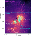 |
Fig. 1 BN/KL outflow and the Trapezium cluster observed with JWST/NIRCam H2 F212N (McCaughrean & Pearson 2023). The dashed square marks the field of view mapped with SOFIA/GREAT. Cyan contours show the [O I] 63 µm redshifted line-wing emission over vLSR = 25–30 km s−1, from 15 to 90 K km s−1 in steps of 15 K km s−1. |
3 SOFIA airborne observations and data reduction
We mapped multiple FIR lines with GREAT during eight SOFIA flights between January 2014 and February 2021. Apart from the flights taking place in in spring 2021 (observing cycle 8), which we operated out of Cologne-Bonn (CGN, Germany) during the pandemic, we carried out all flights from Palmdale, California. We conducted all observations during GREAT Consortium time (project IDs: 83_0004 (cycle 1), 83_0428 (cycle 4), and 83_0630 (cycles 8–9). The flights accumulated 5 hours of observing time.
In 2014, we carried out the first observations of the OH 2Π3/2 J=5/2-3/2 line (2514.3 GHz ≃ 119.2 µm) with the single-pixel detector of GREAT (Heyminck et al. 2012). In 2021, we extended the map using the corresponding channel of the multi-color 4GREAT receiver (Duran et al. 2021). We observed the [O I] 3P1–3P2 line (4744.8 GHz ≃ 63 µm) with the 7-pixel high-frequency array (HFA) of upGREAT (Risacher et al. 2018). We simultaneously observed the [C II] 2P3/2–2P1/2 line (1900.5 GHz ≃ 158 µm) and the [O I] 3P0–3P1 line (2060.1 GHz ≃ 145 µm) with the two polarization-split upGREAT low-frequency sub-arrays (LFA): the 7-pixel V-polarization array tuned to the [O I] line and the H-polarization array to the [C II] line. This configuration processed 21 signals in parallel. We employed Fast Fourier Transform spectrometers, updated from Klein et al. (2012), which provided 32k channels across the ∼0.5–4 GHz intermediate-frequency bands. Table A.1 summarizes the instrument configurations.
The instrument and observatory performance (flight altitude, precipitable water vapor) determined the actual observing mode and source coverage (map sizes), while previous Herschel spectroscopic maps of Goicoechea et al. (2015a) guided them. We reference all observations to the nominal source position RA = 05h35m14.3s, Dec = −05°22′33.7″ (J2000) in the hot core region. We performed the upGREAT observations of both [O I] lines and [C II] in fast total power on-the-fly slewing mode (0.4 sec integration time per dump), using 3″ sampling in both RA and Dec We observed the source twice, scanning once in Dec and once in RA, with the fine sampling driven by the 6.3″ beam of the HFA. The map size (144″×126″) refers to the on-sky coverage of the central array pixels, while the hexagonal array’s outer pixels provide a larger coverage. We selected a “clean” on-sky reference position at ∆RA, ∆Dec=(−1700″, +900″). To achieve the most uniform sampling, we tilted the array axis by 19.1° relative to the scanning direction (Risacher et al. 2016a). We observed the OH 2Π1/2 (1834.7 GHz ≃ 163.4 µm) line during the LFA commissioning in 2016, using chopped (1 Hz) on-the-fly mode with 6″ spatial sampling. The reference OH line frequencies (Table A.1) correspond to the line-strength-weighted frequency of each hyperfine-structure triplet, which are spectrally unresolved. We observed the OH 163.4 µm line of the Λ-doublet in the upper sideband, thereby avoiding to blend with the 163.1 µm line of the doublet in our dual sideband receiver.
We applied a large chop throw of 240″ toward negative RA offsets. Observing the OH 2Π3/2 119.2 µm line proved most challenging. At this frequency, the shortage of local oscillator power needed to pump the HEB mixers forced us to couple the signal via a Martin–Puplett interferometer (Heyminck et al. 2012); this, in turn, limited the receiving bandwidth of the sky signal to ∼1.6 GHz. Thus, the expected velocity coverage of the outflow barely fits into the effective bandpass (∼190 km s−1). This required pointed (raster) observations, in double-beam chopped mode, for optimal system stability (wobbler throw 300″, at −20° counter-clockwise against positive RA). In 2014, an exploratory 5×5 raster on a 10″ grid was observed (with the single-pixel M-channel of GREAT), showing the emission to be compact; in 2021 with 4GREAT we added a 5×5 raster on a 6″ grid.
The GREAT consortium derived the half-power main beam sizes and efficiencies from planet observations. Telescope operators established the pointing on nearby optical reference stars with an accuracy of 1–2″. At the beginning of each flight series, we aligned the instrument’s optical axis with these imagers by observing planets. Although the co-alignment between the central pixels is better than 1–2″ (and the data header accounts for it), we generally tracked the highest frequency channel in a given configuration – typically the central HFA pixel in most flights. We amplitude-calibrated the raw data with the KOSMA kalibrate software (Guan et al. 2012). We corrected the data for atmospheric extinction and calibrated them in Tmb2. When SOFIA flew between 12.2–13.4 km in altitude, the atmospheric transmission remained smooth near the target velocities.
We processed the calibrated data with GILDAS3. We inspected the data to remove noisy spectra and other artifacts (e.g., spikes from onboard interference). We smoothed the spectra to a channel resolution of 0.15 km s−1 (0.3 km s−1 for the OH 119 µm line) and removed first-order baselines. The spectra were then gridded into a data cube through a convolution with a Gaussian kernel of a full width at half maximum (FWHM) of ∼1/3 of the telescope beamwidth at the different frequencies. The 1σ rms noise in the maps are ∼3.5 K ([O I] 63 µm), ∼2.5 K ([O I] 145 µm), and ∼2.0 K ([C II] 158 µm), and ∼4.3 K (OH 163 µm) per velocity channel (as provided by the NOISE routine). To determine the noise over a given velocity bin, we used  , where σch is the rms per channel, δvch the channel width, and Nch the number of channels in that bin. For specific applications (e.g., line intensity ratio maps), we convolved the data cubes with Gaussian kernels to a common angular resolution, corresponding to FWHMs of 13″ or 15″.
4 Results
Figure 1 shows the core of OMC-1 observed with JWST/NIRCam F212N (McCaughrean & Pearson 2023), dominated by H2 v = 1–0 S (1) line emission at 2.12 µm. The dashed square marks the field of view mapped with SOFIA/GREAT, encompassing the wide-angle BN/KL outflow, including the bright Peak 1 and Peak 2 regions. The cyan contours in Fig. 1 show the [O I] 63 µm redshifted line-wing emission at ∼20 km s−1 relative to the cloud systemic velocity of ≃8–9 km s−1 (hereafter vLSR,0; Bally et al. 1987; Berné et al. 2014). This [O I] emission peaks close to BN (Sect. 4.3) and follows the H2 emission from the outflow. The field also includes the massive stars of the Trapezium cluster, in the foreground, located at ∼0.2 pc in front of the cloud. Their far-UV (FUV; 6 < E < 13.6 eV) radiation, dominated by θ1 Ori C star, illuminates all surfaces of OMC-1.
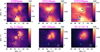 |
Fig. 2 Total line intensity maps (in erg s−1 cm−2 sr−1 = “cgs”) integrated over the complete line profile. The beam size is indicated in the bottom-right corner of each panel except for H2, where it is too small to display (0.1″). The cyan triangle shows a position near the Trapezium, where the [O I] 63µm line intensity peaks (Table D.1). The H2 image refers to the JWST/NIRCam F212N image (McCaughrean & Pearson 2023). The CO J = 10–9 map was obtained with Herschel/HIFI at 20″ resolution (Goicoechea et al. 2019). |
 |
Fig. 3 Total line intensity ratio maps (derived from line intensities in erg s−1 cm−2 sr−1). (a) [O I] 63/145 at a common angular resolution of 13″, (b) [O I] 63/[C II] 158 at 15″, and (c) [O I] 145/ [C II]158 at 15″. The dashed box shows the (100″×80″) area used to extract both the line luminosities in the outflow region (Table 2) and the line intensities as a function of velocity (see Figs. 7 and 8). Contours show the FIR 79 µm-continuum obtained with Herschel/PACS, from 2.5 to 10 (103 Jy), centered at the position of the hot core (Goicoechea et al. 2015a). |
4.1 Integrated line intensity maps
Figure 2 shows [O I] 63 145 µm, [C II] 158 µm, and OH 163 µm total line intensity maps (integrated over their complete line profile) in units of erg s−1 cm−2 sr−1, which are used to compare the emitted line luminosity and line cooling budget. In these maps we mark the positions of key stars (BN and source I) and environments (Peak 1, Peak 2, and the Trapezium region), which we study throughout the manuscript. The [O I] 63 µm emission is the brightest FIR atomic fine-structure line in the region and roughly follows the H2 emission along the wide-angle outflow. Still, the line intensity peaks southwest of the Trapezium stars, hereafter the “Trapezium position,” at (+20″, −50″) from the map center (see details in Sect. 4.2). This region is part of the large-scale, face-on photodissociation region (PDR), with nH ≳ 105 cm−3 (e.g., Herrmann et al. 1997; Goicoechea et al. 2015b, 2019), at the interfaces between OMC-1 and the foreground H II region, which is photoionized by θ1 Ori C. This PDR component is located closer to the observer than the BN/KL outflow and produces bright narrow line emission – often called the “spike” component – at nearly all positions in the field.
The [O I] 145 µm line is strikingly bright and as bright as the [C II] 158 µm line, displaying a similar spatial distribution as the [O I] 63 µm emission. As observed before (e.g., Goicoechea et al. 2015b; Morris et al. 2016), the [C II] 158 µm integrated intensity map does not follow the H2 emission. Instead, [C II] 158 µm shows strong emission close to the Trapezium, along with lower line intensity emission from the FUV-irradiated surface of OMC-1. The OH 2Π1/2 J=3/2-1/2 line emission at 163 µm is confined to the outflow, peaking toward the inner hot core region, with only very faint emission from the quiescent cloud and PDR. The spatial distribution of the OH 163 µm emission resembles that of the high-J CO emission (e.g., Peng et al. 2012; Goicoechea et al. 2015a, 2019).
Figure 3 shows the atomic fine-structure line intensity ratio maps (integrated over the entire line profile). Typically, these intensity ratios provide diagnostics of the gas density, temperature, and FUV radiation field strength in the warm gas associated with PDRs and shocks. Although these maps do not reveal the velocity structure of the gas, they display a different spatial distribution compared to the absolute line intensity maps (Fig. 2). The [O I] 63/[C II] 158 intensity ratio map shows a clear maximum (≃20) toward Peak 1 (Fig. 3b). The [O I] 145/[C II] 158 map exhibits a similar spatial distribution, with a high ratio (≳1) toward Peak 1 (Fig. 3c). Given the much higher critical densities for collisional excitation of the [O I] 63 and 145 µm lines compared to that of the [C II] 158 µm line (see Table A.1), these peaks trace the highest density gas (assuming similar FUV illumination). In general, the [O I] 63/[C II] 158 µm line intensity ratios toward Peak 1 are higher than those observed toward protostellar outflows (e.g., Liseau et al. 2006) and PDRs (e.g., Bernard-Salas et al. 2012). Figure 3 (contours) also shows the FIR continuum map at 79 µm (Goicoechea et al. 2015b), tracing the extended warm dust emission from the hot core region. The continuum emission is fainter toward the Peak 1 and Peak 2. The [O I] 63/145 ratio shows its lowest values (≃10) in a region roughly orthogonal to the wide-angle outflow (Fig. 3a), following the quiescent cloud, the “extended ridge”. Radiative transfer models (Sect. 5.2) indicate that the low intensity ratios are consistent with the [O I] 63 µm line being optically thick, and with the gas having lower density than in the post-shock gas.
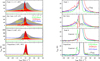 |
Fig. 4 Velocity-resolved spectra at representative positions, all from maps convolved to 15″ (except CO 10–9, with a beam of 20″). Left: Complete spectra, with offsets in arcseconds given in parenthesis; continuum levels of [C II] 158 µm and [O I] 145 µm shifted for clarity. The OH 163 µm emission lines (yellow) are scaled by a factor of three or five. Right: zoom on faint line wings and foreground line features. |
4.2 Velocity-resolved far-IR line profiles
4.2.1 Line wings
The GREAT maps enable us to resolve the velocity structure of the [O I] 63 and 145 µm emission and to compare it with other FIR lines: [C II] 158 µm, OH, and high-J CO. Figure 4 presents such a comparison for four representative positions: Peak 1, the hot core region, Peak 2, and the Trapezium position. The first three positions lie on the outflow region and show line wing emission. As is apparent from these spectra, the OH and CO lines exhibit similarly broad line profiles, with ∆vFWHM ≳ 30 km s−1. These lines reveal prominent wings, with full widths at zero intensity (FWZI) exceeding 150 km s−1 (see Fig. 5 and Kwan & Scoville 1976; Zapata et al. 2009; Peng et al. 2012, for additional velocity-resolved CO studies). These line profiles differ markedly from those of the FIR atomic fine-structure lines (Fig. 4), which consist of a bright narrow component, ∆vFWHM ≃ 4 km s−1, together with moderately broad wings. This suggests that the shocks producing the atomic fine-structure emission differ in nature or location from those driving the highest velocity CO and OH emission.
The FWZI of the [O I] 63 and 145 µm lines toward Peak 1 is ∼85 km s−1 and ∼62 km s−1, respectively. The [O I] FWZIs exceed that of the [C II] 158 µm line (≲ 50 km s−1). This implies that the highest velocity component either lacks FUV illumination or that C+ is rapidly converted into other species in the post-shock gas (see also Morris et al. 2016). The [O I] 145 µm line is optically thin and is not affected by foreground absorptions (see Sect. 4.2.3). Toward Peak 1, the [O I] 145 µm line profile can be fitted with two Gaussians of similar intensity but different line FWHM: a narrow one (∆vFWHM ≃ 3.6 ± 0.1 km s−1 centered at vLSR ≃ +8.2 ± 0.1 km s−1), consistent with gas in the quiscent face-on PDR, and a broad one (∆vFWHM ≃ 19.6 ± 0.3 km s−1 at vLSR ≃ +7.4 ± 0.1 km s−1), implying supersonic velocity dispersions associated with shocked gas.
In Appendix B, we show the velocity channel maps of the observed FIR lines. As in Fig. 1, the redshifted [O I] 63 and 145 µm emission follows the H2 and CO emission along the two lobes of the wide-angle outflow, whereas the red-shifted [C II] 158 µm emission is weak toward Peak 1 and Peak 2 (Fig. B.1). The [O I] 63 and 145 µm emission from the blueshifted wing peaks around BN and Peak 1. At vLSR,0, the atomic lines show extended emission in the SW–NE direction, orthogonal to the wide-angle outflow, mostly tracing the illuminated rim of OMC-1’s ridge.
Assuming that most of the narrow-line emission arises from the face-on PDR at the rims of OMC-1, as suggested by its spatial distribution, we estimate that ∼65%, ∼50%, and ∼15% of the observed [O I] 63, [O I] 145, and [C II] 158 µm emissions, respectively, originate from shocked gas. Nonetheless, some of the narrow line emission may originate from low-velocity outflows or from shocks oblique to the line of sight, so the above percentages should be considered lower limits.
4.2.2 [O I] 63 µm narrow-line “spike” emission
For bright, optically thick [O I] 63 µm emission, the continuum-subtracted peak main-beam temperature, TP = J(Tex) − J(Tdust), where J(T) is the Planck-corrected radiation temperature, yields the excitation temperature, Tex, of the line, arising here from the extended PDR in front of the outflow:
![Mathematical equation: ${T_{{\rm{ex}}}}([{\rm{OI}}]{\rm{63\mu m}}) = {{227.7} \over {\ln \left( {1 + {{227.7} \over {{T_{\rm{P}}}([{\rm{OI}}]{\rm{63\mu m}}) + J({T_{{\rm{dust}}}})}}} \right)}}{\rm{K}},$](/articles/aa/full_html/2026/06/aa58900-26/aa58900-26-eq3.png) (1)
(1)
where ∆E/kB = (Eu − El)/kB = 227.7 K, and J(Tdust) = Tc is the continuum brightness temperature at 63 µm. In most observed positions, TP([OI] 63 µm) ≃ 100–120 K, and J(Tdust) ≃ 5–100 K (from the 63 µm continuum levels of Werner et al. 1984), where the highest value refers to the hot core region. These TP([OI] 63 µm) values translate to Tex ≳ 200 K, which is a lower limit to the gas temperature (e.g., Fig. C.2).
Far from the outflow, the atomic fine-structure lines are narrow and lack high-velocity wings. This is exemplified by the spectra toward the Trapezium position (Fig. 4), where these lines show Gaussian profiles and line FWHM of about 5 km s−1 (Table D.1). Still, this particular position – resembling a cavity structure – shows remarkably strong [O I] 63 µm emission, with a peak brightness temperature of Tpeak = 330 K (at the native 6″ resolution). This implies Tk ≥ Tex ≃ 440 K (with Tc ≃ 5 K, and assuming a beam filling of one), consistent with warm-to-hot gas in a dense PDR facing the Trapezium. This excited PDR is located near the region of maximum CH+ J = 1–0 emission in OMC-1 (position #3 of Goicoechea et al. 2019), a signature of strong FUV irradiation and elevated temperatures. JWST images reveal this and similar cavities illuminated by FUV radiation from the Trapezium; e.g., Fig. 4 of McCaughrean & Pearson (2023) and Fig. 4 of Habart et al. (2024). These “crenellations” (O’Dell et al. 2015) at OMC-1’s illuminated surface were likely carved by protostellar outflows (see also Kavak et al. 2022).
4.2.3 Foreground [O I] 63 µm line absorption
The [O I] 63 µm line is a ground-state transition. The strong dust continuum at 63 µm from the central BN/KL region (Werner et al. 1976; Cernicharo et al. 2006; Goicoechea et al. 2015b), together with the presence of low excitation gas along the line of sight, produces absorption features in the blueshifted [O I] 63 µm line wing, where Tex < Tc. In this region, the [O I] 63 µm line profile shows a narrow, a few km s−1 FWHM, absorption component at vLSR ≃ +6 km s−1, which is typically associated with gas in the hot core itself (e.g., Blake et al. 1987; Tercero et al. 2010). In addition, it shows blueshifted absorptions, at vLSR ≃ −1 km s−1 (toward Peak 1) and at vLSR ≃ +2 km s−1 (toward the hot core and Peak 2). These blueshifted absorptions coincide with [C II] 158 µm emission peaks (left panels of Fig. 4) known to arise from foreground material in Orion’s Veil (Goicoechea et al. 2015b; Pabst et al. 2019), including the “Northern Dark Lane” and the “Dark Bay”, which are apparent in optical images (O’Dell 2001). Because of the lower density in these components (nH ≈ 103 cm−3; Pabst et al. 2020), the fainter 158 µm continuum, and the much lower critical density of the [C II] 158 µm transition, leading to Tex > Tc, these foreground gas layers appear as [C II] 158 µm emission components. Away from the hot core region, the [O I] 63 µm line profiles show no absorption components.
4.2.4 OH P-Cygni profiles from the high-velocity outflow
Figure 4 (left panel, yellow histograms) display the OH 2Π1/2 J=3/2-1/2 line profile (one of the Λ-doublets of the excited OH 163 µm transition). These observations have much higher angular and spectral resolution than previous observations with the Kuiper Airborne observatory (KAO), the Infrared Space Telescope (ISO), and Herschel (Melnick et al. 1987, 1990; Goicoechea et al. 2006a, 2015a). The OH 163 µm line profile toward Peak 1 shows a very broad profile, with a FWZI of ≳ 150 km s−1 and ∆vFWHM ≃ 40 km s−1, thus comparable to the CO lines (e.g., Kwan & Scoville 1976; Snell et al. 1984; Zapata et al. 2009; Peng et al. 2012; Bally et al. 2017). As opposed to the atomic fine-structure lines, the OH 163 µm emission does not show a narrow line component. Indeed, the line is very faint toward the Trapezium position (Fig. 4), implying that the broad-line emission originates in shocked gas and regions that are subject to strong radiative pumping, but not from the quiescent cloud gas. This rotationally excited OH line arises from the first excited state (at Eu/k = 270 K) of the 2Π1/2 ladder. Given its high excitation requirements (ncr ≃ 109 cm−3), the upper level can only be populated by collisions in very dense, warm gas, and/or by absorption of FIR dust photons in the 2Π1/2–2Π3/2 cross-ladder transition at ∼53 µm (e.g., Goicoechea & Cernicharo 2002; Goicoechea et al. 2006a). Owing to the different dust continuum levels, the latter process contributes to the hot core region, while the former likely dominates in Peak 1 and Peak 2, with possible lateral (i.e., not along the line of sight) FIR illumination from the hot core. The broad OH 163 µm line profiles trace the outflow at all velocities, and the line intensity tends to peak toward the hot core (see also Fig. B.1), where the effect of FIR pumping is strongest.
Figure 5 compares the [O I] 63 µm, CO J = 10–9, and OH 2Π3/2 J=5/2-3/2 (one of the Λ-doublets of the OH 119 µm ground-state transition) line profiles toward the hot core position (roughly the FIR dust continuum peak). The [O I] 63 µm spectrum shows the three absorption components at vLSR ≃ +6, +2, and −1 km s−1. The first component is consistent with gas in the hot core, while the other two originate from foreground gas associated with Orion’s Veil. Betz & Boreiko (1989) provided the first sub-km s−1 resolution observations of the OH 119 µm rotational line with the KAO. These observations revealed a self-absorption profile, characterized by absorption on the blueshifted side and emission on the redshifted side. The SOFIA telescope delivers a factor of three better angular resolution (11.3″ at 119 µm), which provides less angular dilution of the FIR continuum source. The resulting OH 119 µm line shows a more prominent P-Cygni profile (the line shows absorption and emission of similar strength), with a FWZI of ≃160 km s−1, much like CO lines. Compared to Betz & Boreiko (1989), SOFIA observations show that the entire blueshifted wing is absorbed from vLSR ≃ −80 to +8.5 km s−1, while the redshifted emission extends up to vLSR ≃ +80 km s−1, with a velocity coverage similar to that of the CO J = 10–9 line. Clearly, OH is present in the high-velocity outflowing gas, with terminal (maximum) velocities of about 80 km s−1 – the fastest gas producing absorption projected along the line of sight. A closer examination of the OH 119 µm P-Cygni profile reveals that the main absorption dip occurs at vLSR ≃ +6 km s−1, which corresponds to the hot core absorption (for a zoomed-in spectrum, see Fig. B.3). We leave a detailed analysis of the OH excitation to a forthcoming paper.
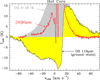 |
Fig. 5 P-Cygni profile of the OH 119 µm line toward the hot core region (the FIR continuum peak), compared to other line profiles. See Fig. B.3 for a zoom on the low-intensity features. |
4.3 A possible outflow or wind bow shock around BN
Figure 6 (left) shows a map of the [O I] 63 µm emission in the vLSR range from +20 to +25 km s−1. In addition to the red-shifted extended emission from the explosive outflow, we detect an emission peak near BN, located slightly northwest (NW) of this young massive star (∼8–13 M⊙; e.g., Rodríguez et al. 2005). This emission does not coincide with the more extended, so-called low-velocity “18 km s−1 outflow,” which expands in the SW–NE direction (Genzel et al. 1981; Plambeck et al. 1982) and is likely driven by Source I (Beuther & Nissen 2008; Wright et al. 2022). The new [O I] 63 µm component arises from a broad emission feature, with a line FWHM of 15 ± 1 km s−1, centered at vLSR ≈ 20 km s−1 (blue spectrum in Fig. 6). This emission is confined to the vicinity of BN, indicating either a compact outflow or a knot or shell of shock-excited gas surrounding the star. It envelops the IR nebulosity associated with BN (see Shuping et al. 2004; Bally et al. 2020) but has not been reported in other line tracers, likely owing to the nature of this shocked gas and the complex substructure of the region in terms of emission, velocity, and extinction.
The centroid of the [O I] 63 µm line feature is compatible with the LSR velocity measured from emission lines associated with BN (vLSR ≃ 23 km s−1; Gómez et al. 2008; Goddi et al. 2011; Plambeck et al. 2013). The apparent extent of this [O I] 63 µm feature is < 10″ and remains undetected at 145 µm. The blue- and redshifted [O I] 63 µm emission around the LSR velocity of BN shows a similar spatial distribution, suggesting that, if it originates from an outflow, the outflow is spatially unresolved. Given the uncertain properties of BN’s circumstellar disk, particularly its geometry (Jiang et al. 2005; Beuther et al. 2010; Bally et al. 2020), it remains unclear whether this structure traces a disk-driven outflow or another form of shocked gas.
Interestingly, the [O I] 63 µm intensity peak is shifted to the NW of BN by ≲3″, and is roughly aligned with the proper motion of this runaway star. Thus, this [O I] 63 µm emission may correspond to an unresolved wind bow shock produced by the interaction of BN’s supersonic motion and wind with the ambient cloud gas (Baranov et al. 1971; Wilkin 1996). Adopting estimates of the wind mass-loss rate (Ṁw), wind velocity (vw), and BN’s velocity (v∗) relative to the surrounding cloud of density n0 (Scoville et al. 1983; Bally et al. 2020), the bow-shock radius (rbs) would be several hundred au, or ≲ 1″ (Tan 2004). However, the wind mass-loss rate and velocity remain uncertain. Since  , larger wind parameters would yield a correspondingly larger rbs (for fixed n0 and v∗), potentially consistent with the apparent size of the [O I] 63 µm feature.
5 Analysis
In the following, we restrict our analysis to a 100″ × 80″ (0.2 pc × 0.16 pc) region around the outflow, indicated with a dashed square in Fig. 3. Specifically, we excluded the Trapezium region. In addition, we used the spectra of Peak 1 as a template to determine the physical conditions of the post-shock gas.
5.1 Velocity-resolved line intensity ratios
Figure 7 shows the FIR line intensity ratios as a function of velocity toward the Peak 1 position (filled squares) obtained from maps convolved to a common angular resolution of 15″. The lowest [O I] 63/145 line intensity ratio, 11.4 ± 0.1, occurs at vLSR,0, corresponding to the LSR velocity of the quiescent gas in OMC-1 (dashed magenta line in Fig. 7), where the narrow line component is dominated by emission from the extended PDR in front of the outflow. This intensity ratio is comparable to that observed in the Orion Bar (e.g., Bernard-Salas et al. 2012). The [O I] 63/145 intensity ratio then increases in the line wings, reaching ∼30 at redshifted velocities. The [O I] 63/145 intensity ratio shows an asymmetry between the blue- and redshifted wings. Foreground [O I] 63 µm absorption at vLSR between roughly −5 and +7 km s−1 contributes to this asymmetry, but the blueshifted wing shows smaller ratios at higher, more negative velocities. These lower ratios suggest a correspondingly lower density in the blueshifted post-shock gas (Sect. 5.2).
Figure 7 also shows the velocity dependence of the [O I] 145/[C II] 158, [O I] 63/[C II] 158, and OH 163/[C II] 158 line intensity ratios. All these ratios reach a minimum at the LSR velocity of the face-on PDR, vLSR,0, and gradually increase in the line wings, indicating a lower contribution of C+ in the highest velocity gas. The [O I] 145 µm line is particularly bright, with [O I] 145/[C II] 158 intensity ratios of ≃2–3 in the line wings. The OH 163/[C II] 158 line intensity ratio increases from ≃0.1 at the line center to 4 ± 1 in the wings, thus showing a strong dependence on radial velocity. The redshifted line wing shows very high [O I] 63/[C II] 158 intensity ratios, up to ≃50–100, much higher than the expected ratios in PDRs with nH ≈ 105 cm−3 (e.g., Kaufman et al. 1999). For reference, in the prototypical dense PDR, the Orion Bar, at ∼2′ south of the Trapezium, these line intensity ratios are much lower, [O I] 63/145 ≃ 9, [O I] 63/[C II] 158 ≃ 8, [O I] 145/[C II] 158 ≃ 0.9, and OH 163/[C II] 158 ≃ 0.03 (e.g., Bernard-Salas et al. 2012; Joblin et al. 2018).
The empty squares in Fig. 7 show the FIR line intensity ratios as a function of LSR velocity, averaged over the 100″ × 80″ region, thus representing the average conditions in the outflow. These ratios are similar to those toward Peak 1, with the main differences being a slightly higher [O I] 63/145 intensity ratio in the blueshifted wing and slightly lower [O I] 145/[C II] 158, [O I] 63/[C II] 158, and OH 163/[C II] 158 ratios. This reflects the higher relative contribution of the [C II] 158 µm emission4 in the SE part of the outflow (see Figs. 3b and 3c). Figure B.2 shows these results in the form of intensity-ratio velocity channel maps. These maps illustrate the same trends described above: the [O I] 63/[C II] 158 and [O I] 145/[C II] 158 ratios in the redshifted wing peak toward Peaks 1 and 2, following the H2 outflow. These regions coincide with enhanced [O I] 63/145 intensity ratios.
Table 1 summarizes the intensities of the atomic fine-structure lines toward Peak 1, measured in three velocity intervals of the line profile: the redshifted wing, the blueshifted wing, and the narrow component. To increase the S/N of the line-intensity measurements and to cover the relevant outflow velocity range, we derived the wing intensities using velocity bins of 25 km s−1 in the wings. We adopted the [+21, +46] and [−30, −5] km s−1 LSR velocity intervals for the redshifted and blueshifted wings, respectively. That is, radial velocities of 13 to 38 km s−1 with respect to vLSR,0. This choice excludes the velocity ranges of the [O I] 63 and [C II] 158 µm lines that are affected by foreground absorption and emission in the blueshifted wing (see Fig. 4). We also subtracted the contribution of the [13C II] F = 2–1 hyperfine-structure line in the redshifted wing using multi-Gaussian fitting. In Sect. 6.2, we use these line-wing intensities to constrain the nature of the shocks that give rise to the FIR atomic line emission.
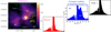 |
Fig. 6 Possible compact outflow or wind bow shock around BN star. Left: spatial distribution of the redshifted [O I] 63 µm emission in the vLSR range from +20 to +25 km s−1. This map (in RA and Dec) shows extended emission following the wide-angle H2 outflow and a possible spatially unresolved outflow around BN, revealed as a distinct broad spectral component. Right: [O I] 63 µm spectra toward Source I (red), BN (blue), and Peak 1 (black). Only the blue spectrum shows the broad spectral feature around the LSR velocity of BN (dashed green line). |
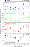 |
Fig. 7 Line intensity ratios as a function of velocity in a 15″ beam toward Peak 1 (filled squares) and averaged over the 100″ × 80″ region of the BN/KL outflow (empty squares), binned in intervals of 5 km s−1 from maps convolved to a common resolution of 15″. The dashed magenta line marks the LSR velocity of the quiescent gas in OMC-1. |
5.2 Post-shock gas physical conditions and [O I]63 145 µm excitation across different outflow velocity components
The observed [O I] 63/[O I] 145 µm intensity ratios (I63/I145) in the line wings are high, reaching up to ∼30 (e.g., Table 1). This is close to the high-temperature limit for optically thin emission under local thermodynamic equilibrium (LTE5) conditions (Tex = Tk). This would imply N(O) < a few 1018 cm−2 and high densities, meaning nH ≫ ncr, with ncr,63µm ≃ 5 × 105 cm−3 and ncr,145µm ≃ 6 × 106 cm−3 for optically thin emission. However, LTE is rarely fulfilled, and even for a three-level system such as the 3PJ levels of oxygen, subtle non-LTE (NLTE), line opacity, and FIR pumping effects can dominate the [O I] emission, thus, the resulting I63/I145 ratio (Monteiro & Flower 1987; Elitzur & Asensio Ramos 2006; Goicoechea et al. 2009; Goldsmith 2019).
To estimate the beam-averaged physical conditions (nH, Tk) and the atomic oxygen column densities, N(O), in the post-shock gas across the different velocity components, we used a nonlocal NLTE radiative transfer model (Goicoechea et al. 2006b, 2009) with up-to-date O–H2 and O–H inelastic collision rate coefficients (Lique et al. 2018). This nonlocal approach accounts for [O I] 63 µm line opacity and line trapping, as well as [O I] 145 µm suprathermal excitation (Tex > Tk) and population inversions, which “local” single escape probability methods fail to correctly capture. To match the observed [O I] 145 µm line FWHM (broad component), we adopted a turbulent line width of 20 km s−1. Following Goicoechea et al. (2009), we also examined the impact of FIR radiative pumping on the [O I] fine-structure level populations. Appendix C provides details and explores the excitation conditions over a wide parameter space.
Figure 8 presents the results of a model grid displayed in the velocity-dependent parameter space I63/I145 (v) versus I145(v). The light grey to black curves show radiative transfer models for four atomic oxygen column densities, from 2×10¹⁶ to 2×1019 cm−2, increasing from left to right, at two gas temperatures, 200 and 500 K. Tick marks denote log nH (in cm−3) and are separated by one decade along curves of constant N(O). In general, as the opacity of the [O I] 63 µm line increases, the intensity ratio I63/I145 decreases roughly as ∼ 1/τ63, while the [O I] 145 µm line is rarely optically thick. In dense gas, intensity ratios I63/I145 ≲ 15 typically imply optically thick [O I] 63 µm emission. For the adopted parameters, the gas density also determines the [O I] excitation regime. For nH ≳ ncrit, the I63/I145 ratio increases with nH owing to a significant increase in the [O I] 63 µm excitation temperature and a decrease in τ63 toward the optically thin regime. In this regime, the ratio also increases with decreasing gas temperature. The colored squares in Fig. 8 represent the observed values in LSR velocity bins of 5 km s−1 toward Peak 1 (filled squares) and averaged over the BN/KL outflow (open squares). Red squares correspond the redshifted line wing, in the range [+10, +25] km s−1, while blue squares correspond to the blueshifted line wing, [−20, 0] km s−1. Green squares in Fig. 8 correspond to the quiescent cloud gas at OMC-1 velocities, vLSR = [+5, +10] km s−1. The green squares are consistent with large column densities of atomic oxygen, N(O) ≃ 1019 cm−2, optically thick [O I] 63 µm emission, nH of several 105 cm−3, and temperatures Tk ≃ 200–400 K – thus compatible with the observed TP([O I]63 µm) values (Sect. 4.2) –, typical of a dense PDR with a thermal pressure, Pth/k, of 107 to 108 K cm−3. This agrees with previous observations of the large-scale PDRs at the surfaces of OMC-1 (Herrmann et al. 1997; Goicoechea et al. 2015b, 2019). An increase in velocity within the line wings (red and blue squares) is accompanied by a rise in the [O I] 63/145 intensity ratio, consistent with higher gas densities and less opaque [O I] 63 µm emission. The lower I145(v) intensities as velocities increase simply reflect smaller N(O) column densities. Toward Peak 1, the [O I] 63 and 145 µm line-wing emission is consistent with nH of several 105 to 106 cm−3, Tk ≲ 500 K, and N(O) of a few 1017 cm−2. Figure 8 also indicates that the post-shock gas density is slightly lower in the blueshifted gas. When averaged over the entire outflow, the I63/I145(v) ratio is highest at the largest velocities, where the H2 and O column densities are lowest. The higher ratios imply nH up to several 106 cm−3, consistent with gas compression in the post-shock gas.
FIR atomic fine-structure line intensities and intensity ratios at different velocities toward Peak 1 and the Orion Bar PDR (for reference).
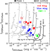 |
Fig. 8 [O I] 63/145 µm intensity ratio versus [O I] 145 µm intensity. The light grey to black curves show a grid of radiative transfer models for four values of N(O): 2×10¹⁶, 2×10¹⁷, 2×10¹⁸, and 2×1019 cm−2, from left to right, at 200 and 500 K. Tick marks denote log nH (in cm−3) and are separated by one decade along curves of constant N(O). The colored squares show the observed values in LSR velocity bins of 5 km s−1 toward Peak 1 (filled squares) and averaged over the BN/KL outflow (open squares). Red squares correspond to the redshifted line wing, while blue squares correspond to the blueshifted line wing. Green squares correspond to OMC-1 velocities (see Tables D.2 and D.3). |
6 Discussion
6.1 Peak 1 as a laboratory for shock modeling
Early models of Peak 1 have required two types of shocks to explain the observations (e.g., Chernoff et al. 1982; Draine & Roberge 1982; Neufeld & Dalgarno 1989; Haas et al. 1991; Kaufman & Neufeld 1996; Le Bourlot et al. 2002; Esplugues et al. 2014). The accepted picture was that a high-velocity molecular flow (the “plateau”) produces nondissociative C-type shocks (with shock velocities vS ≳ 25 km s−1) as the flow interacts with the ambient molecular cloud, generating high temperatures (above 1000 K). These shocks lead to bright H2 and high-J CO emission along with large H2O/CO > 1 abundance ratios. Newer C-type shock models included the effects of modest external UV illumination (Melnick & Kaufman 2015) to explain the unusual detection of narrow-line O2 toward Peak 1 (Chen et al. 2014). In addition, fast, vS = 70–80 km s−1, dissociative, J-type shocks were proposed to occur where a high-velocity wind impacts the expanding swept-up material (Hollenbach 1985), producing bright atomic fine-structure line emission. However, BN/KL’s explosive outflow is driven by bullets moving through the molecular cloud (e.g., Bally et al. 2015, 2020), rather than by stellar jets or winds, as in protostellar outflows. In Sect. 6.2 we explore the nature of the shocks driving the atomic fine-structure emission.
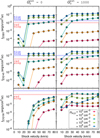 |
Fig. 9 FIR atomic line intensities as a function of shock velocity and preshock gas density (from Lehmann et al. 2022). The right panels show externally irradiated shocks. The horizontal blue and red lines indicate the observed line-wing intensities toward Peak 1 (Table 1). |
6.2 Nature of the [O I]–emitting shocks
Figure 9 compares the intensities of the [O I] 63 µm, [O I] 145 µm, and [C II] 158 µm lines observed in the red and blue wings toward Peak 1 (Table 1) with those predicted by the Paris–Durham shock code6 (Godard et al. 2019) along the direction perpendicular (face-on) to the shock front. In this comparison, we assume an emission beam filling factor of f = 1. The models are from Lehmann et al. (2022), which account for magnetized molecular shocks with velocities in the range vS = 5–80 km s−1, preshock gas densities in the range nH,0 = 102–106 cm−3, enabling us to include an external FUV field  , in units of the Mathis field (Mathis et al. 1983).
The strength of the preshock magnetic field prior to the explosion is uncertain. Dust polarimetric observations of the plane-of-sky magnetic field in the quiescent cloud indicate values of a few hundred µG (Houde et al. 2009; Guerra et al. 2021), consistent with line-of-sight field strengths derived from CN Zeeman measurements (Crutcher et al. 1999; Crutcher 1999). Thus, all models in Fig. 9 adopt a reference magnetic parameter b = 1, where the preshock transverse magnetic field strength is given by B = b (nH,0/cm−3)1/2 µG. For this range of parameters, shocks can be of type C, C∗, or CJ at vS < 25 km −1, or J-type at vS > 25 km−1 (Lehmann et al. 2020, 2022). The models assume either  (left panels) or
  (right panels). Accurately determining the flux of external FUV photons reaching each bow-shock structure–whether locally self-generated, generated in nearby shocks, emitted by massive protostars within the region (BN, source I, and source n; Shuping et al. 2004), or originating from the Trapezium stars–is challenging, as it depends on both the porosity of the medium and the properties of the shocks and the protostars. The representative value of
  lies within the very rough estimates from FIR continuum observations toward Peak 1 (Goicoechea et al. 2015a).
In the absence of external irradiation  , the predicted [O I] line intensities converge toward a plateau at high shock velocities, the level of which is primarily set by the preshock gas density. This is consistent with the dissociative shock models of Hollenbach & McKee (1989). Shocks with sufficiently high velocities generate a local FUV radiation field (e.g., Lehmann et al. 2020), whose intensity scales as
 (2)
(2)
for 30 < vS ≲ 100 km s−1 (Lehmann et al. 2020; Godard et al. 2024), and thus strongly depend on vS . At low shock velocities, models with  underpredict the observed [C II] 158 µm intensity by several orders of magnitude. Marginally reproducing the [C II]158 µm intensity would require very fast shocks, vS ≳ 80 km s−1. However, this is in contradiction with the ∆vFWHM and FWZI values of the observed fine-structure lines (Sect. 4.2), assuming that the flow is roughly directed along the line of sight. Therefore, a significant contribution from locally self-generated UV radiation is unlikely.
External FUV radiation, which leads to carbon photoionization and CO photodissociation, significantly enhances the intensities of atomic fine-structure lines (right panels of Fig. 9). Still, owing to the enhanced importance of C+ recombination and chemical destruction at high gas densities, the [C II] 158 µm intensity does not increase monotonically with density.
Under external irradiation, the observations no longer constrain a unique set of shock parameters, but are instead consistent with a family of solutions involving J-type shocks with vS ≃ 30–40 km s−1 and nH,0 ≳ a few 104 cm−3. Models with  reproduce the [C II] 158 µm intensity of the redshifted wing, tracing gas moving into OMC-1, whereas the blueshifted wing emission, tracing gas moving toward the Trapezium, appears to require higher values of
  . In the following, we focus on the redshifted wing emission.
In these irradiated shocks, the predicted I63/I158 line intensity ratio primarily scales with the preshock gas density and shows only a weak dependence on the shock velocity for vS > 30 km s−1 (see Fig. 10). The above family of solutions predicts I63/I158 ≳ 60, consistent with the redshifted wing emission toward Peak 1, which shows intensity ratios up to ∼50–100 (Fig. 7). Given the inferred post-shock densities from the [O I] excitation analysis in Sect. 5.2, nH of several 105 to 106 cm−3, the resulting compression factors, F = nH/nH,0 ≳ 30, also support magnetized J-type shocks, where F ∼ vS /b (Godard et al. 2024). The compressed magnetic field would have a strength of several mG, similar to the values observed toward BN/KL (Pattle et al. 2017; Guerra et al. 2021). All in all, the [O I] and [C II] line-wing emission is best reproduced by externally irradiated, dissociative J-type shocks with velocities of 30–40 km s−1, preshock densities of a few 104 cm−3, and compression factors consistent with post-shock densities derived from the [O I] excitation analysis.
A more detailed interpretation would require the geometry, time dependence, and spatial variations of b and  across the outflow to be fully accounted for. Still, the results shown in Fig. 9 provide a general interpretative framework: dense bullets, with proper motions up to several hundred km s−1, accelerated by the explosion event (i.e., Doi et al. 2002; Bally et al. 2015, 2017), interact with the ambient molecular cloud, generating bow-shock structures seen in [Fe II] knots and H2 (Fig. 1). The highest bullet velocities exceed the observed FWZIs of the CO and OH lines, and imply molecular gas dissociation and the production of significant FUV radiation in many bow-shock tips (Eq. (2)). Within this framework, surrounding fast shocks generate sufficient external FUV radiation to illuminate the inner layers of the bow-shock structures. The working surfaces of these bow shocks drive dissociative J-type shocks with velocities of a few tens of km s−1, producing the observed [O I] emission.
Consistently with this scenario, the observed H I 21 cm line emission from atomic hydrogen (produced after H2 (photo)dissociation) extends only up to vLSR ≤ 31 km s−1 (see Fig. 20 of van der Werf et al. 2013) and broadly resembles the [O I] 63 µm emission, both in its spatial distribution and in its lack of the highest velocity emission seen in CO or OH. The broader CO and OH line profiles indicate that the shocks responsible for their emission differ from those driving the atomic fine-structure emission. For instance, Melnick & Kaufman (2015) concluded that a C-shock with vS = 23 km s−1 propagating into a more shielded molecular clump (preshock density of 8 × 104 cm−3 and  ) explains the detection of O2 (Chen et al. 2014).
We conclude that, in contrast to what was found using previous models (e.g., Hollenbach & McKee 1989; Haas et al. 1991), fast shocks with vS ≃ 70–80 km, s−1 are not required to explain the observed atomic fine-structure line intensities and profiles. Instead, the observed lines are consistent with lower velocity, dissociative J-type shocks illuminated by external FUV radiation, with  , depending on the shock parameters (e.g., Kristensen et al. 2023). This radiation arises from surrounding fast shocks and possibly from nearby massive (proto)stars, enhancing the [C II] 158 µm emission, particularly in blueshifted gas moving toward the cluster.
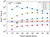 |
Fig. 10 [O I] 63/[C II] 158 µm line intensity ratio as a function of shock velocity and preshock gas density in an externally irradiated shock with |

Total IR line luminosities in the BN/KL outflow region†.
6.3 Mass-loss rate of the explosive outflow in Orion BN/KL
The energy loss from the outflow-driven shock provides a measure of the kinetic (mechanical) luminosity of the outflow, with  . In this expression7, Lcool is the total shock cooling rate and (1 − fm) denotes the fraction of the shock mechanical energy translated into internal excitation. In general, gas cooling proceeds through IR, H I, and optical line emission, Lcool ≈ LIR + LHI + Loptical, where
  is the contribution from atomic fine-structure lines, H2 lines, and other molecular lines (CO, H2O, OH, etc.). LHI and Loptical are only relevant in dissociative J-type shocks (Lehmann et al. 2020). LHI represents the hydrogen-line cooling emission (e.g., Lyα, Lyβ, and two-photon continuum) and Loptical refers to “optical” atomic forbidden-line emission, which arises from electronic transitions in the visible and NIR. From the above relation7,
 (3)
(3)
where fIR is the fraction of the total cooling due to IR emission lines. In general, fIR ≈ 0.5–0.8 in C-type shocks (e.g., Kaufman et al. 1999; Karska et al. 2025) and fIR ≈ 0.5 in J-type shocks (e.g., Lehmann et al. 2020). Equation (3) has clear limitations when different types of shocks coexist, or when part of the emitted line luminosity arises from FUV-heated gas. In the following analysis, we assume that vS ≃ 30–40 km s−1 represents the velocity range of the possible shock types in BN/KL’s outflow (if more than one), whether dissociative or nondissociative. Table 2 summarizes the IR line luminosities, integrated over the entire profile, across the outflow (dashed square in Fig. 3). Inserting the outflow IR line luminosity, LIR ≃ 320 L⊙, Eq. (3) yields a mass-loss rate of Ṁ0 ≃ (9.1 ± 2.6) × 10−3 M⊙ yr−1, using fIR = 0.5 (Fig. 3 of Lehmann et al. 2020) and (1 − fm) = 0.75 (Kaufman & Neufeld 1996). Even if the derived Ṁ0 is an approximate value, the estimated mass-loss rate of BN/KL’s outflow is higher than that of steady protostellar outflows. Given a dynamical timescale of tdyn ≃ 500 yr (e.g., Zapata et al. 2009), the derived outflow mass is M = tdyn Ṁ0 ≃ (3.3–5.9) M⊙. This estimate agrees with, yet may be more accurate than, mass estimates obtained from column densities computed under the LTE assumption (Snell et al. 1984; Peng et al. 2012). Still, future theoretical work should revisit the validity of Eq. (3) in the complex scenario described in Sect. 6.2, considering its dependence on multiple shocks and  .
.
[O I] 63, 145 µm and FIR CO line luminosities toward the central emission (a size of ∼0.2 pc) of several high-mass star-forming regions.
6.4 Mass-loss rate from the putative BN outflow
Here, we assume that the spatially unresolved [O I] 63 µm emission detected around BN – both spatially and in LSR velocity (see Sect. 4.3) – arises from shocked gas produced by a compact outflow launched by this star. When [O I] 63 µm is the dominant gas coolant in a J-type “wind” shock–consistent with detection of this outflow only in [O I] 63 µm–Hollenbach (1985) showed that the line luminosity scales with the outflow mass-loss rate as Ṁ (M⊙ yr−1) ≃ 10−4 L63 (L⊙), provided that the flux of material into the shock satisfies nH,0 vS ≲ 1012 cm−2 s−1. In this regime, the particle flux is related to the [O I] 63 µm line intensity by nH,0 vS ≃ 1013 I63, with nH,0, vS , and I63 in cgs units.
The broad [O I] 63 µm line emission around BN is characterized by I63 ≃ 5×10⁻² erg s−1 cm−2 sr−1 and L63 ≃ 0.6 L⊙ in ≲ 4000 au. Thus, its contribution to the total L63 of the entire map is negligible. Using the relations above, we obtain, nH,0 vS ≃ 5×1011 cm−2 s−1 and Ṁ ≃ 6 × 10⁻⁵ M⊙ yr−1, which is typical of accreting high-mass protostars (e.g., Beuther et al. 2002; Leurini et al. 2015). Assuming further that the shock velocity is comparable to the [O I] 63 µm line FWHM of the spectral component around BN, ∆vFWHM ≃ 15 km s−1 (Sect. 4.3), we derive a preshock gas density of several 105 cm−3. These results indicate that the kinematics, density, and mass-loss rate associated with the compact [O I] 63 µm emission around BN are consistent with a disk-accretion–driven outflow originating from BN. Further observations of additional tracers at high angular resolution will be needed to confirm the outflow versus wind bow shock scenario, or to constrain alternative interpretations.
6.5 Comparison with other high-mass star-forming regions
To investigate whether explosive outflows produce distinct spectroscopic features, here we compare the observed FIR [O I], [C II], and CO line luminosities of the BN/KL outflow with those measured in the central regions of other, more distant high-mass star-forming regions where similar observations have been carried out (e.g., Leurini et al. 2015). In the BN/KL outflow region, the FIR atomic line luminosity is dominated by [O I] 63 µm8, which is ∼15 times brighter than the [C II] 158 µm emission. The total [O I] 63 µm and 145 µm line luminosity is remarkably high, 86.5 L⊙, comparable to the total H2 and CO luminosity (Rosenthal et al. 2000; Goicoechea et al. 2015a). This yields L[OI]/LCO ≃ 0.9 and ![Mathematical equation: ${L_{[{\rm{OI}}]}}/{L_{{{\rm{H}}_2}}} \simeq 0.7$](/articles/aa/full_html/2026/06/aa58900-26/aa58900-26-eq22.png) . That is, about 25% of the total IR gas cooling is through [O I] emission lines (Table 2). Furthermore, the contribution to L[OI] from the broad spectral component, neglecting the narrow spike [O I] emission, is 55 L⊙.
. That is, about 25% of the total IR gas cooling is through [O I] emission lines (Table 2). Furthermore, the contribution to L[OI] from the broad spectral component, neglecting the narrow spike [O I] emission, is 55 L⊙.
Table 3 compares the FIR line luminosities toward the central regions of several high-mass star-forming regions, on scales of ∼0.2 pc comparable to our BN/KL map. Interestingly, interferometric observations of the central regions of DR21 and G5.89−0.39 reveal CO outflows exhibiting fingers and Hubble-Lemaître flow kinematics, consistent with the presence of explosive outflows (e.g., Zapata et al. 2013, 2020; Guzmán Ccolque et al. 2024). These other regions exhibit fractional luminosities comparable to those of BN/KL outflow, both displaying high LOI/Lbol and  ratios, ≳10−4. In contrast, W3-IRS5, a proto-Trapezium system (e.g., Rodón et al. 2008), and NGC7538-IRS1, a massive star-forming core hosting an ultracompact H II region, a late O–to–early B star (Sandell & Sievers 2004), exhibit lower LOI/Lbol and
  luminosities. Pending more robust statistics, these high fractional luminosities may represent a distinctive signature of explosive outflows.
Still, the BN/KL outflow stands out in FIR [O I] and CO line surface luminosities, per unit area, and the I63/I158 intensity ratios exceed those in most regions, even when integrating over the full line profile, suggesting a denser gas environment.
7 Summary and conclusions
In this paper, we present velocity-resolved, sub-km s−1- resolution maps of the [O I] 63 and 145 µm fine-structure emission lines along the wide-angle explosive outflow in Orion BN/KL. We complement this data with new [C II] 158 µm and FIR OH line maps, all obtained with the GREAT heterodyne receivers on board SOFIA. Our main conclusions are as follows:
We separated the quiescent and the outflow (broad [O I] line-wing) components, with the latter following the shock-excited H2 emission and the former primarily tracing the foreground, face-on PDR at the UV-illuminated rims of OMC-1. The [O I] 63 µm line has a FWZI of ∼85 km s−1. The FWZI of the [C II] 158 µm line is smaller, ≲ 50 km s−1, implying that either the highest velocity gas lacks FUV illumination or (more likely) C+ is quickly converted into other species;
The broad [O I] 145 µm component (∆vFWHM ≃ 20 km s−1) is narrower than the corresponding CO and OH emission (∆vFWHM ≳ 30 km s−1), which also exhibit larger FWZIs (≳ 150 km s−1). This suggests that the shocks producing the [O I] emission differ either in their nature or in exact location from those driving the highest velocity CO and OH emission;
The [O I] 63/145 and [O I] 63/[C II] 158 intensity ratios attain remarkably high values in the line wings (20–30 and 40–60, respectively), exceeding those observed in PDRs and typical protostellar outflows. They are consistent with dense (nH ≳ 105–106 cm−3) and warm (T ≲ 500 K) post-shock gas;
The fine-structure line-wing emission is consistent with originating in externally irradiated, magnetized, dissociative J-type shocks with vS ≃ 30–40 km s−1 and preshock densities of a few 104 cm−3. External FUV radiation arises from surrounding fast shocks and possibly from massive (proto)stars in the region if the medium is sufficiently porous;
The [O I] 63 and 145 µm luminosity along the outflow region is significantly high, amounting to 86.5 L⊙, with 55 L⊙ contributed by the broad component alone. This is comparable to the H2 and CO line luminosities, yielding L[OI]/LCO ≃ 0.9 and
![Mathematical equation: ${L_{[{\rm{OI}}]}}/{L_{{{\rm{H}}_2}}} \simeq 0.7$](/articles/aa/full_html/2026/06/aa58900-26/aa58900-26-eq25.png) . These values imply an outflow mass-loss rate of (9.1 ± 2.6) × 10−3 M⊙ yr−1 and a mass of M ≃ (3.3–5.9) M⊙;
. These values imply an outflow mass-loss rate of (9.1 ± 2.6) × 10−3 M⊙ yr−1 and a mass of M ≃ (3.3–5.9) M⊙;We report the detection of broad [O I] 63 µm emission, slightly offset from BN but aligned with the direction of the star’s proper motion. This L63 ≃ 0.6 L⊙ emission could arise from an unresolved outflow (corresponding to a mass-loss rate of several 10−5 M⊙ yr−1) or a wind bow shock produced by the supersonic motion of this wind-blowing runaway B star.
The FIR [C II] and [O I] line intensities are among the brightest tracers of interstellar shocks and PDRs, probing the thermal budget and the presence of FUV radiation. In addition, sub-km s−1-resolution maps reveal the gas dynamics, allowing us to quantify the contributions of radiative and mechanical feedback. Unfortunately, given the cessation of SOFIA operations, very-high-spectral-resolution mapping has been carried out for only a few regions of the sky. Therefore, a FIR heterodyne mission (airborne or space) would be the only telescope to provide this essential missing information.
Acknowledgements
We thank our referee for a constructive report that allowed us to improve the presentation of our work. This work is based on observations made with SOFIA (NASA/DLR). SOFIA was jointly operated by the Universities Space Research Association, Inc. (USRA), under NASA contract NAS2-97001, and the Deutsches SOFIA Institut (DSI) under the DLR contract 50 OK 0901 and 50 OK 1301 to the University of Stuttgart. GREAT was a development by the MPI für Radioastronomie and the KOSMA/Universität zu Köln, in cooperation with the DLR Institut für Optische Sensorsysteme. GREAT development was financed by the participating institutes, by DLR under Grants 50 OK 1102, 1103, and 1104, and within the Collaborative Research Centre 956, funded by the Deutsche Forschungsgemeinschaft (DFG). JRG, MGSM, and MZ thank the Spanish MICIU for funding support under grant PID2023-146667NB-I00. MZ acknowledges the JdC Postdoctoral Fellowship JDC2024-054658-I, funded by MICIU/AEI/10.13039/501100011033 and by the ESF+. BG and AG acknowledge the support from the Programme National “Physique et Chimie du Milieu Interstellaire” (PCMI) of CNRS/INSU with INC/INP funded by CEA and CNES.
References
- Allen, D. A., & Burton, M. G. 1993, Nature, 363, 54 [Google Scholar]
- Bally, J. 2008, Overview of the Orion Complex, ed. B. Reipurth, 459 [Google Scholar]
- Bally, J., & Zinnecker, H. 2005, AJ, 129, 2281 [NASA ADS] [CrossRef] [Google Scholar]
- Bally, J., Langer, W. D., Stark, A. A., & Wilson, R. W. 1987, ApJ, 312, L45 [NASA ADS] [CrossRef] [Google Scholar]
- Bally, J., Cunningham, N. J., Moeckel, N., et al. 2011, ApJ, 727, 113 [NASA ADS] [CrossRef] [Google Scholar]
- Bally, J., Ginsburg, A., Silvia, D., & Youngblood, A. 2015, A&A, 579, A130 [NASA ADS] [CrossRef] [EDP Sciences] [Google Scholar]
- Bally, J., Ginsburg, A., Arce, H., et al. 2017, ApJ, 837, 60 [Google Scholar]
- Bally, J., Ginsburg, A., Forbrich, J., & Vargas-González, J. 2020, ApJ, 889, 178 [NASA ADS] [CrossRef] [Google Scholar]
- Baranov, V. B., Krasnobaev, K. V., & Kulikovskii, A. G. 1971, Sov. Phys. Dokl., 15, 791 [NASA ADS] [Google Scholar]
- Beckwith, S., Persson, S. E., Neugebauer, G., & Becklin, E. E. 1978, ApJ, 223, 464 [Google Scholar]
- Bernard-Salas, J., Habart, E., Arab, H., et al. 2012, A&A, 538, A37 [NASA ADS] [CrossRef] [EDP Sciences] [Google Scholar]
- Berné, O., Marcelino, N., & Cernicharo, J. 2014, ApJ, 795, 13 [CrossRef] [Google Scholar]
- Betz, A. L., & Boreiko, R. T. 1989, ApJ, 346, L101 [NASA ADS] [CrossRef] [Google Scholar]
- Beuther, H., & Nissen, H. D. 2008, ApJ, 679, L121 [Google Scholar]
- Beuther, H., Schilke, P., Sridharan, T. K., et al. 2002, A&A, 383, 892 [NASA ADS] [CrossRef] [EDP Sciences] [Google Scholar]
- Beuther, H., Linz, H., Bik, A., Goto, M., & Henning, T. 2010, A&A, 512, A29 [NASA ADS] [CrossRef] [EDP Sciences] [Google Scholar]
- Blake, G. A., Sutton, E. C., Masson, C. R., & Phillips, T. G. 1987, ApJ, 315, 621 [Google Scholar]
- Cernicharo, J., Goicoechea, J. R., Daniel, F., et al. 2006, ApJ, 649, L33 [Google Scholar]
- Chen, J.-H., Goldsmith, P. F., Viti, S., et al. 2014, ApJ, 793, 111 [NASA ADS] [CrossRef] [Google Scholar]
- Chernoff, D. F., Hollenbach, D. J., & McKee, C. F. 1982, ApJ, 259, L97 [Google Scholar]
- Crutcher, R. M. 1999, ApJ, 520, 706 [NASA ADS] [CrossRef] [Google Scholar]
- Crutcher, R. M., Troland, T. H., Lazareff, B., Paubert, G., & Kazès, I. 1999, ApJ, 514, L121 [Google Scholar]
- Doi, T., O’Dell, C. R., & Hartigan, P. 2002, AJ, 124, 445 [Google Scholar]
- Draine, B. T. 1980, ApJ, 241, 1021 [NASA ADS] [CrossRef] [Google Scholar]
- Draine, B. T., & Roberge, W. G. 1982, ApJ, 259, L91 [Google Scholar]
- Duran, C. A., Gusten, R., Risacher, C., et al. 2021, IEEE Trans. Terahertz Sci. Technol., 11, 194 [CrossRef] [Google Scholar]
- Elitzur, M., & Asensio Ramos, A. 2006, MNRAS, 365, 779 [Google Scholar]
- Esplugues, G. B., Viti, S., Goicoechea, J. R., & Cernicharo, J. 2014, A&A, 567, A95 [NASA ADS] [CrossRef] [EDP Sciences] [Google Scholar]
- Geballe, T. R., Burton, M. G., & Pike, R. E. 2017, ApJ, 837, 83 [NASA ADS] [CrossRef] [Google Scholar]
- Genzel, R., & Stutzki, J. 1989, ARA&A, 27, 41 [CrossRef] [Google Scholar]
- Genzel, R., Reid, M. J., Moran, J. M., & Downes, D. 1981, ApJ, 244, 884 [Google Scholar]
- Gerin, M., Ruaud, M., Goicoechea, J. R., et al. 2015, A&A, 573, A30 [NASA ADS] [CrossRef] [EDP Sciences] [Google Scholar]
- Godard, B., Pineau des Forêts, G., Lesaffre, P., et al. 2019, A&A, 622, A100 [NASA ADS] [CrossRef] [EDP Sciences] [Google Scholar]
- Godard, B., des Forêts, G. P., & Bialy, S. 2024, A&A, 688, A169 [NASA ADS] [CrossRef] [EDP Sciences] [Google Scholar]
- Goddi, C., Humphreys, E. M. L., Greenhill, L. J., Chandler, C. J., & Matthews, L. D. 2011, ApJ, 728, 15 [Google Scholar]
- Goicoechea, J. R., & Cernicharo, J. 2002, ApJ, 576, L77 [NASA ADS] [CrossRef] [Google Scholar]
- Goicoechea, J. R., Cernicharo, J., Lerate, M. R., et al. 2006a, ApJ, 641, L49 [NASA ADS] [CrossRef] [Google Scholar]
- Goicoechea, J. R., Pety, J., Gerin, M., et al. 2006b, A&A, 456, 565 [NASA ADS] [CrossRef] [EDP Sciences] [Google Scholar]
- Goicoechea, J. R., Compiègne, M., & Habart, E. 2009, ApJ, 699, L165 [Google Scholar]
- Goicoechea, J. R., Chavarría, L., Cernicharo, J., et al. 2015a, ApJ, 799, 102 [NASA ADS] [CrossRef] [Google Scholar]
- Goicoechea, J. R., Teyssier, D., Etxaluze, M., et al. 2015b, ApJ, 812, 75 [Google Scholar]
- Goicoechea, J. R., Santa-Maria, M. G., Bron, E., et al. 2019, A&A, 622, A91 [NASA ADS] [CrossRef] [EDP Sciences] [Google Scholar]
- Goldsmith, P. F. 2019, ApJ, 887, 54 [NASA ADS] [CrossRef] [Google Scholar]
- Gómez, L., RodrÍguez, L. F., Loinard, L., et al. 2005, ApJ, 635, 1166 [CrossRef] [Google Scholar]
- Gómez, L., Rodríguez, L. F., Loinard, L., et al. 2008, ApJ, 685, 333 [CrossRef] [Google Scholar]
- González-Alfonso, E., Wright, C. M., Cernicharo, J., et al. 2002, A&A, 386, 1074 [NASA ADS] [CrossRef] [EDP Sciences] [Google Scholar]
- Guan, X., Stutzki, J., Graf, U. U., et al. 2012, A&A, 542, L4 [NASA ADS] [CrossRef] [EDP Sciences] [Google Scholar]
- Guerra, J. A., Chuss, D. T., Dowell, C. D., et al. 2021, ApJ, 908, 98 [NASA ADS] [CrossRef] [Google Scholar]
- Guzmán Ccolque, E., Fernández López, M., Zapata, L. A., Bally, J., & Rivera-Ortiz, P. R. 2024, A&A, 689, A339 [NASA ADS] [CrossRef] [EDP Sciences] [Google Scholar]
- Haas, M. R., Hollenbach, D., & Erickson, E. F. 1991, ApJ, 374, 555 [Google Scholar]
- Habart, E., Peeters, E., Berné, O., et al. 2024, A&A, 685, A73 [NASA ADS] [CrossRef] [EDP Sciences] [Google Scholar]
- Herrmann, F., Madden, S. C., Nikola, T., et al. 1997, ApJ, 481, 343 [CrossRef] [Google Scholar]
- Heyminck, S., Graf, U. U., Güsten, R., et al. 2012, A&A, 542, L1 [NASA ADS] [CrossRef] [EDP Sciences] [Google Scholar]
- Hollenbach, D. 1985, Icarus, 61, 36 [NASA ADS] [CrossRef] [Google Scholar]
- Hollenbach, D., & McKee, C. F. 1979, ApJS, 41, 555 [Google Scholar]
- Hollenbach, D., & McKee, C. F. 1989, ApJ, 342, 306 [Google Scholar]
- Houde, M., Vaillancourt, J. E., Hildebrand, R. H., Chitsazzadeh, S., & Kirby, L. 2009, ApJ, 706, 1504 [Google Scholar]
- Jiang, Z., Tamura, M., Fukagawa, M., et al. 2005, Nature, 437, 112 [Google Scholar]
- Joblin, C., Bron, E., Pinto, C., et al. 2018, A&A, 615, A129 [NASA ADS] [CrossRef] [EDP Sciences] [Google Scholar]
- Karska, A., Herpin, F., Bruderer, S., et al. 2014, A&A, 562, A45 [NASA ADS] [CrossRef] [EDP Sciences] [Google Scholar]
- Karska, A., Figueira, M., Mirocha, A., et al. 2025, A&A, 697, A186 [NASA ADS] [CrossRef] [EDP Sciences] [Google Scholar]
- Kaufman, M. J., & Neufeld, D. A. 1996, ApJ, 456, 611 [NASA ADS] [CrossRef] [Google Scholar]
- Kaufman, M. J., Wolfire, M. G., Hollenbach, D. J., & Luhman, M. L. 1999, ApJ, 527, 795 [Google Scholar]
- Kavak, Ü., Goicoechea, J. R., Pabst, C. H. M., et al. 2022, A&A, 660, A109 [NASA ADS] [CrossRef] [EDP Sciences] [Google Scholar]
- Klein, B., Hochgürtel, S., Krämer, I., et al. 2012, A&A, 542, L3 [NASA ADS] [CrossRef] [EDP Sciences] [Google Scholar]
- Kristensen, L. E., Ravkilde, T. L., Field, D., Lemaire, J. L., & Pineau Des Forêts, G. 2007, A&A, 469, 561 [NASA ADS] [CrossRef] [EDP Sciences] [Google Scholar]
- Kristensen, L. E., Ravkilde, T. L., Pineau Des Forêts, G., et al. 2008, A&A, 477, 203 [CrossRef] [EDP Sciences] [Google Scholar]
- Kristensen, L. E., Godard, B., Guillard, P., Gusdorf, A., & Pineau des Forêts, G. 2023, A&A, 675, A86 [NASA ADS] [CrossRef] [EDP Sciences] [Google Scholar]
- Kwan, J. & Scoville, N. 1976, ApJ, 210, L39 [Google Scholar]
- Le Bourlot, J., Pineau des Forêts, G., Flower, D. R., & Cabrit, S. 2002, MNRAS, 332, 985 [NASA ADS] [CrossRef] [Google Scholar]
- Lehmann, A., Godard, B., Pineau des Forêts, G., & Falgarone, E. 2020, A&A, 643, A101 [EDP Sciences] [Google Scholar]
- Lehmann, A., Godard, B., Pineau des Forêts, G., Vidal-García, A., & Falgarone, E. 2022, A&A, 658, A165 [CrossRef] [EDP Sciences] [Google Scholar]
- Lerate, M. R., Barlow, M. J., Swinyard, B. M., et al. 2006, MNRAS, 370, 597 [CrossRef] [Google Scholar]
- Lesaffre, P., Pineau des Forêts, G., Godard, B., et al. 2013, A&A, 550, A106 [NASA ADS] [CrossRef] [EDP Sciences] [Google Scholar]
- Leurini, S., Wyrowski, F., Wiesemeyer, H., et al. 2015, A&A, 584, A70 [NASA ADS] [CrossRef] [EDP Sciences] [Google Scholar]
- Lique, F., Kłos, J., Alexander, M. H., Le Picard, S. D., & Dagdigian, P. J. 2018, MNRAS, 474, 2313 [NASA ADS] [CrossRef] [Google Scholar]
- Liseau, R., Justtanont, K., & Tielens, A. G. G. M. 2006, A&A, 446, 561 [NASA ADS] [CrossRef] [EDP Sciences] [Google Scholar]
- Lonsdale, C. J., Becklin, E. E., Lee, T. J., & Stewart, J. M. 1982, AJ, 87, 1819 [Google Scholar]
- Maret, S., Bergin, E. A., Neufeld, D. A., et al. 2009, ApJ, 698, 1244 [NASA ADS] [CrossRef] [Google Scholar]
- Mathis, J. S., Mezger, P. G., & Panagia, N. 1983, A&A, 128, 212 [NASA ADS] [Google Scholar]
- McCaughrean, M. J., & Mac Low, M.-M. 1997, AJ, 113, 391 [Google Scholar]
- McCaughrean, M. J., & Pearson, S. G. 2023, arXiv e-prints [arXiv:2310.03552] [Google Scholar]
- Melnick, G. J., & Kaufman, M. J. 2015, ApJ, 806, 227 [NASA ADS] [CrossRef] [Google Scholar]
- Melnick, G. J., Genzel, R., & Lugten, J. B. 1987, ApJ, 321, 530 [NASA ADS] [CrossRef] [Google Scholar]
- Melnick, G. J., Stacey, G. J., Genzel, R., Lugten, J. B., & Poglitsch, A. 1990, ApJ, 348, 161 [Google Scholar]
- Menten, K. M., & Reid, M. J. 1995, ApJ, 445, L157 [Google Scholar]
- Menten, K. M., Reid, M. J., Forbrich, J., & Brunthaler, A. 2007, A&A, 474, 515 [NASA ADS] [CrossRef] [EDP Sciences] [Google Scholar]
- Monteiro, T. S., & Flower, D. R. 1987, MNRAS, 228, 101 [Google Scholar]
- Morris, P. W., Gupta, H., Nagy, Z., et al. 2016, ApJ, 829, 15 [NASA ADS] [CrossRef] [Google Scholar]
- Neufeld, D. A., & Dalgarno, A. 1989, ApJ, 344, 251 [Google Scholar]
- Nissen, H. D., Cunningham, N. J., Gustafsson, M., et al. 2012, A&A, 540, A119 [NASA ADS] [CrossRef] [EDP Sciences] [Google Scholar]
- O’Dell, C. R. 2001, ARA&A, 39, 99 [Google Scholar]
- O’Dell, C. R., Ferland, G. J., Henney, W. J., et al. 2015, AJ, 150, 108 [CrossRef] [Google Scholar]
- Pabst, C., Higgins, R., Goicoechea, J. R., et al. 2019, Nature, 565, 618 [NASA ADS] [CrossRef] [Google Scholar]
- Pabst, C. H. M., Goicoechea, J. R., Teyssier, D., et al. 2020, A&A, 639, A2 [NASA ADS] [CrossRef] [EDP Sciences] [Google Scholar]
- Pattle, K., Ward-Thompson, D., Berry, D., et al. 2017, ApJ, 846, 122 [Google Scholar]
- Peng, T.-C., Wyrowski, F., Zapata, L. A., Güsten, R., & Menten, K. M. 2012, A&A, 538, A12 [NASA ADS] [CrossRef] [EDP Sciences] [Google Scholar]
- Plambeck, R. L., Wright, M. C. H., Welch, W. J., et al. 1982, ApJ, 259, 617 [Google Scholar]
- Plambeck, R. L., Bolatto, A. D., Carpenter, J. M., et al. 2013, ApJ, 765, 40 [Google Scholar]
- Risacher, C., Güsten, R., Stutzki, J., et al. 2016a, A&A, 595, A34 [NASA ADS] [CrossRef] [EDP Sciences] [Google Scholar]
- Risacher, C., Güsten, R., Stutzki, J., et al. 2016b, IEEE Trans. Terahertz Sci. Technol., 6, 199 [CrossRef] [Google Scholar]
- Risacher, C., Güsten, R., Stutzki, J., et al. 2018, J. Astron. Instrum., 7, 1840014 [NASA ADS] [CrossRef] [Google Scholar]
- Rodríguez, L. F., Poveda, A., Lizano, S., & Allen, C. 2005, ApJ, 627, L65 [CrossRef] [Google Scholar]
- Rodón, J. A., Beuther, H., Megeath, S. T., & van der Tak, F. F. S. 2008, A&A, 490, 213 [NASA ADS] [CrossRef] [EDP Sciences] [Google Scholar]
- Rosenthal, D., Bertoldi, F., & Drapatz, S. 2000, A&A, 356, 705 [NASA ADS] [Google Scholar]
- Sandell, G., & Sievers, A. 2004, ApJ, 600, 269 [NASA ADS] [CrossRef] [Google Scholar]
- Schöier, F. L., van der Tak, F. F. S., van Dishoeck, E. F., & Black, J. H. 2005, A&A, 432, 369 [Google Scholar]
- Scoville, N., Kleinmann, S. G., Hall, D. N. B., & Ridgway, S. T. 1983, ApJ, 275, 201 [Google Scholar]
- Shuping, R. Y., Morris, M., & Bally, J. 2004, AJ, 128, 363 [Google Scholar]
- Snell, R. L., Scoville, N. Z., Sanders, D. B., & Erickson, N. R. 1984, ApJ, 284, 176 [NASA ADS] [CrossRef] [Google Scholar]
- Stacey, G. J., Jaffe, D. T., Geis, N., et al. 1993, ApJ, 404, 219 [NASA ADS] [CrossRef] [Google Scholar]
- Tan, J. C. 2004, ApJ, 607, L47 [Google Scholar]
- Tercero, B., Cernicharo, J., Pardo, J. R., & Goicoechea, J. R. 2010, A&A, 517, A96 [NASA ADS] [CrossRef] [EDP Sciences] [Google Scholar]
- Tielens, A. G. G. M., & Hollenbach, D. 1985, ApJ, 291, 747 [NASA ADS] [CrossRef] [Google Scholar]
- van der Tak, F. F. S., Chavarría, L., Herpin, F., et al. 2013, A&A, 554, A83 [NASA ADS] [CrossRef] [EDP Sciences] [Google Scholar]
- van der Werf, P. P., Goss, W. M., & O’Dell, C. R. 2013, ApJ, 762, 101 [NASA ADS] [CrossRef] [Google Scholar]
- Werner, M. W., Gatley, I., Harper, D. A., et al. 1976, ApJ, 204, 420 [Google Scholar]
- Werner, M. W., Crawford, M. K., Genzel, R., et al. 1984, ApJ, 282, L81 [Google Scholar]
- Wilkin, F. P. 1996, ApJ, 459, L31 [Google Scholar]
- Wright, M., Bally, J., Hirota, T., et al. 2022, ApJ, 924, 107 [Google Scholar]
- Young, E. T., Becklin, E. E., Marcum, P. M., et al. 2012, ApJ, 749, L17 [NASA ADS] [CrossRef] [Google Scholar]
- Youngblood, A., France, K., Ginsburg, A., Hoadley, K., & Bally, J. 2018, ApJ, 857, 7 [Google Scholar]
- Zapata, L. A., Schmid-Burgk, J., Ho, P. T. P., Rodríguez, L. F., & Menten, K. M. 2009, ApJ, 704, L45 [Google Scholar]
- Zapata, L. A., Schmid-Burgk, J., Pérez-Goytia, N., et al. 2013, ApJ, 765, L29 [NASA ADS] [CrossRef] [Google Scholar]
- Zapata, L. A., Ho, P. T. P., Fernández-López, M., et al. 2020, ApJ, 902, L47 [Google Scholar]
- Zapata, L. A., Fernández-López, M., Leurini, S., et al. 2023, ApJ, 956, L35 [CrossRef] [Google Scholar]
The German REceiver for Astronomy at Terahertz frequencies was developed by the MPI für Radioastronomie and the KOSMA/Universität zu Köln, in cooperation with the DLR Institut für Optische Sensorsysteme.
We shall refer to the “line luminosity” (L) in erg s−1 or L⊙ units. The conversion from integrated line intensity (W = ∫ ∆Tmb dv) in K km s−1, where ∆Tmb is the continuum-subtracted main brightness temperature, to integrated line intensity (I) in erg s−1 cm−2 sr−1 is I = 2k W ν3/c3, or I(erg s−1 cm−2 sr−1) = W(K km s−1)·ν(GHz)3/9.76·1014.
The [C II] 158 µm emission around vLSR ≃ +20 km s−1 can be dominated by [13C II] F = 2–1 emission from OMC-1 (right panels of Fig. 4).
In the optically thin LTE regime,  , where [E(3P0)−E(3P1)]/k = 98.8 K (see also Goldsmith 2019).
Available on the ISM platform https://ism.obspm.fr
This equation is written in the reverse form compared to that used in some outflow papers (e.g., Maret et al. 2009), such that Lkin ≥ Lcool.
Goicoechea et al. (2015a) derived L[OI]63 ≃ 16 L⊙ from Herschel/PACS maps using a nonstandard engineering observing mode to avoid saturation. This is a factor ∼5 lower than the SOFIA/GREAT value. Although we do not find an obvious explanation for this discrepancy, the SOFIA luminosities are more consistent with KAO luminosities, L[OI]63 = 50 ± 25 L⊙ (Werner et al. 1984).
Appendix A Observed lines, instrument configurations, and observing modes
Table A.1 summarizes the instrument configurations, observing parameters, and observed FIR line properties.
Observed lines, instrument configurations, and observing modes.
The observing modes are indicated: total power (TP) or chopped (ch) on-the-fly (OTF: data is acquired while slewing the telescope), or raster mode (the telescope stays pointed while integrating). The size of a given map is quoted for the central array pixel only; the step between dumps (along the scanning direction) and between adjacent OTF slews is given or the grid used for pointed raster observations.
Appendix B Complementary observational figures
This appendix presents additional figures that aim to better understand the velocity structure of BN/KL outflow.
Appendix B.1 Velocity channel maps
Figure B.1 shows velocity-channel maps (in K km s−1 units) of the FIR lines observed with SOFIA and the CO J = 10–9 line observed with Herschel/HIFI (Goicoechea et al. 2019).
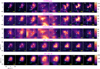 |
Fig. B.1 Velocity channel maps at their native angular resolution and in K km s−1 intensity units, from vLSR = −10 to +25 km s−1 in bins of 5 km s−1 [v, v + 5], with v indicated in the bottom-right corner of each panel. The map at v = +5 km s−1 shows the emission at the systemic velocity of the quiescent gas in OMC-1, vLSR,0 ≃ 8–9 km s−1, dominated by extended emission from a face-on PDR. The main reference positions discussed in the text are illustrated with symbols (see Fig. 2). |
Figure B.2 shows channel maps of line intensity ratios for the different FIR atomic lines (with intensities in cgs units).
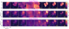 |
Fig. B.2 Velocity-resolved line intensity ratio channel maps (same velocity bins as in Fig. B.1) convolved at a common angular resolution of 15″, with the integrated line intensities in erg s−1 cm−2 sr−1. The map at v = +5 km s−1 shows the emission at the systemic velocity of the quiescent gas. |
Appendix B.2 Line profiles toward the FIR continuum peak
Figure B.3 (right panel) shows a zoom on the low-intensity features of several FIR lines toward the FIR continuum peak position (the hot core region), with the main [O I] 63 µm absorption and [C II] 158 µm emission features labelled.
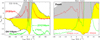 |
Fig. B.3 OH 119 µm P-Cygni profile toward the hot core (FIR continuum peak), compared to other line profiles. The OH 119 µm absorption dip agrees with [O I] 63 µm absorption at +6 km s−1 (hot core velocities). The [C II] 158 µm emission and [O I] 63 µm absorption at +2 km s−1 corresponds to a gas structure in the foreground. |
Appendix C Nonlocal NLTE [O I] radiative transfer models
In our [O I] excitation and radiative transfer models (Goicoechea et al. 2006b, 2009), we adopted the fine-structure O–H2 and O–H collisional rate coefficients calculated by Lique et al. (2018) in the 10–1000 K temperature range. As observed, the FIR [O I] fine-structure line emission in the outflow arises from molecular gas with some atomic H (van der Werf et al. 2013). Hence, we define the gas density as nH = n(H) + 2n(H2), and adopted n(H2)/n(H) ≃ 4 in the models. We verified that this choice does not affect our main conclusions and results. We ran spherical models with uniform gas densities (nH = 104–108 cm−3), temperatures (Tk = 200 and 500 K, based on the observed Tmb([O I] 63 µm) line peaks), and a fixed velocity dispersion, σturb = 8.5 km s−1 (i.e., ∆vturb,FWHM ≃ 20 km s−1), matching the observed [O I] 145 µm broad component toward Peak 1.
Figure C.1 shows the results of the grid, displaying I145 as a function of nH (left panels) for different atomic oxygen column densities: 2 × 10¹⁷, 2 × 10¹⁸, and 2 × 1019 cm−2, and gas temperatures. The right panels shows the resulting I63/I145 line intensity ratio as a function of nH. Continuos curves refer to models without external FIR illumination. The red and cyan colored areas show the I63/I145 ratios measured toward Peak 1 in the red- and blueshifted wings, respectively (extracted from Table 1). These ratios are consistent with the presence of dense (nH ≃ several 105 to 106 cm−3) and warm (T ≲ 500 K) post-shock gas, with N(O) ≃ a few 1018 cm−2.
In these plots, the opacity of the [O I] 63 µm line increases as N(O) increases, from optically thin to thick emission. That is, from high to low densities–from right to left in the figures–as collisional excitation becomes less important and the low energy levels become more populated. This is reflected in very sub-thermal [O I] 63 µm excitation (Tex,63 µm ≪ Tk) when nH ≪ ncr,63 µm (Fig. C.2, left panels). Figure C.2 shows the average Tex,63 µm and Tex,145 µm in the models, but we note that due to radiative transfer effects—such as line trapping—the local Tex values vary with position, even under uniform physical conditions. The excitation of the [O I] 145 µm line is more complex and is governed by the spontaneous radiative decay of the upper level (3P0), which is roughly five times lower than that of the lower level (3P1). In addition, the collisional de-excitation rate coefficient for O–H2 collisions of the 3P0–3P1 (145 µm) transition is significantly smaller than that of the 3P1–3P2 (63 µm) transition (e.g., Monteiro & Flower 1987; Lique et al. 2018). These properties lead to [O I] 145 µm population inversions (Tex,145 µm < 0 K) at low densities (nH < ncr,145 µm) and suprathermal emission (Tex,145 µm > Tk) at high densities (previously discussed by Liseau et al. 2006; Elitzur & Asensio Ramos 2006; Goicoechea et al. 2009; Goldsmith 2019). These features are evident in the right panels of Fig. C.2.
To investigate the role of FIR pumping in the [O I] excitation, the dotted curves in Figs. C.2 and C.1 represent the same models but adding external FIR continuum illumination. We model the continuum background as the sum of the cosmic microwave background and a modified blackbody, η B(Td)(1 − exp(−τd,λ)), at a dust color temperature of Td = 100 K. In this expression, η is the filling factor of the background FIR continuum emission, which we set to 0.5. The dust continuum emission is assumed to be optically thick at 100 µm, with τd,λ = 7 [100/λ(µm)]2, and represents the typical FIR dust continuum emission close to the hot core region (see Goicoechea et al. 2015a). The main role of this FIR continuum is to produce [O I] 63 µm line absorption (when Tex < Tcont) at low gas densities, nH below a few 104 cm−3, as the [O I] 63 µm line becomes optically thick, for N(O) ≳ 1018 cm−2.
In general, FIR pumping increases the population of the 3P1 level (in this case increasing the excitation temperature of the [O I] 63 µm line; see dotted curves in Fig. C.2, left), thereby reducing the population inversion of the 3P0–3P1 transition at [O I] 145 µm. At low to moderate gas densities, the [O I] 63 µm line intensity decreases, whereas the intensity of the [O I] 145 µm remains nearly unchanged. Consequently, the I63/I145 intensity ratio is slightly lower (dotted curves in Fig. C.1, right) than in the nonilluminated case. Hence, the inferred post-shock gas density may be slightly higher.
At high densities, however, the main effect of FIR pumping is to slightly reduce Tex,145 µm, although it remains suprathermal (Fig. C.2, right), leading to a slightly higher I63/I145 intensity ratio (Fig. C.1, right).
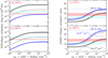 |
Fig. C.1 Nonlocal and NLTE [O I] excitation and radiative transfer models: Predicted [O I] 145 µm line intensity (left) and [O I] 63/145 µm intensity ratio in cgs units (right) as a function of total gas density. The black, grey, and blue curves represent different column densities of atomic oxygen. Dotted curves represent models with external FIR illumination (see text). In the left panels, the red and cyan dashed lines show the [O I]145 µm intensities measured toward Peak 1 in the red- and blueshifted wings, respectively. In the right panels, the red and cyan dashed colored areas show the intensity ratios (with errors) measured toward Peak 1 in the red- and blueshifted wings, respectively (see Table 1). |
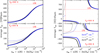 |
Fig. C.2 Average excitation temperature of the [O I] 63 µm and [O I] 145 µm lines as a function of gas density for two gas temperatures, 200 and 500 K. The black, grey, and blue curves represent different column densities of atomic oxygen, indicated in the right panel. Dotted curves represent models with external FIR illumination (see text). The increase in the [O I] 63 µm excitation temperature at low densities reflects the role of FIR pumping by a modified black body at Td = 100 K. This effect reduces the population inversion of the transition at 145µm at low densities. |
Appendix D Line intensity tables
In this appendix we tabulate the FIR line intensities toward the Trapezium position and Peak 1, as well as the average line intensities over the entire outflow region.
Results of Gaussian fits to FIR lines toward the narrow [O I] 63 µm line intensity peak near the Trapezium, at an offset of (+20″, −50″).
All Tables
FIR atomic fine-structure line intensities and intensity ratios at different velocities toward Peak 1 and the Orion Bar PDR (for reference).
[O I] 63, 145 µm and FIR CO line luminosities toward the central emission (a size of ∼0.2 pc) of several high-mass star-forming regions.
Results of Gaussian fits to FIR lines toward the narrow [O I] 63 µm line intensity peak near the Trapezium, at an offset of (+20″, −50″).
All Figures
|
Fig. 1 BN/KL outflow and the Trapezium cluster observed with JWST/NIRCam H2 F212N (McCaughrean & Pearson 2023). The dashed square marks the field of view mapped with SOFIA/GREAT. Cyan contours show the [O I] 63 µm redshifted line-wing emission over vLSR = 25–30 km s−1, from 15 to 90 K km s−1 in steps of 15 K km s−1. |
| In the text | |
|
Fig. 2 Total line intensity maps (in erg s−1 cm−2 sr−1 = “cgs”) integrated over the complete line profile. The beam size is indicated in the bottom-right corner of each panel except for H2, where it is too small to display (0.1″). The cyan triangle shows a position near the Trapezium, where the [O I] 63µm line intensity peaks (Table D.1). The H2 image refers to the JWST/NIRCam F212N image (McCaughrean & Pearson 2023). The CO J = 10–9 map was obtained with Herschel/HIFI at 20″ resolution (Goicoechea et al. 2019). |
| In the text | |
|
Fig. 3 Total line intensity ratio maps (derived from line intensities in erg s−1 cm−2 sr−1). (a) [O I] 63/145 at a common angular resolution of 13″, (b) [O I] 63/[C II] 158 at 15″, and (c) [O I] 145/ [C II]158 at 15″. The dashed box shows the (100″×80″) area used to extract both the line luminosities in the outflow region (Table 2) and the line intensities as a function of velocity (see Figs. 7 and 8). Contours show the FIR 79 µm-continuum obtained with Herschel/PACS, from 2.5 to 10 (103 Jy), centered at the position of the hot core (Goicoechea et al. 2015a). |
| In the text | |
|
Fig. 4 Velocity-resolved spectra at representative positions, all from maps convolved to 15″ (except CO 10–9, with a beam of 20″). Left: Complete spectra, with offsets in arcseconds given in parenthesis; continuum levels of [C II] 158 µm and [O I] 145 µm shifted for clarity. The OH 163 µm emission lines (yellow) are scaled by a factor of three or five. Right: zoom on faint line wings and foreground line features. |
| In the text | |
|
Fig. 5 P-Cygni profile of the OH 119 µm line toward the hot core region (the FIR continuum peak), compared to other line profiles. See Fig. B.3 for a zoom on the low-intensity features. |
| In the text | |
|
Fig. 6 Possible compact outflow or wind bow shock around BN star. Left: spatial distribution of the redshifted [O I] 63 µm emission in the vLSR range from +20 to +25 km s−1. This map (in RA and Dec) shows extended emission following the wide-angle H2 outflow and a possible spatially unresolved outflow around BN, revealed as a distinct broad spectral component. Right: [O I] 63 µm spectra toward Source I (red), BN (blue), and Peak 1 (black). Only the blue spectrum shows the broad spectral feature around the LSR velocity of BN (dashed green line). |
| In the text | |
|
Fig. 7 Line intensity ratios as a function of velocity in a 15″ beam toward Peak 1 (filled squares) and averaged over the 100″ × 80″ region of the BN/KL outflow (empty squares), binned in intervals of 5 km s−1 from maps convolved to a common resolution of 15″. The dashed magenta line marks the LSR velocity of the quiescent gas in OMC-1. |
| In the text | |
|
Fig. 8 [O I] 63/145 µm intensity ratio versus [O I] 145 µm intensity. The light grey to black curves show a grid of radiative transfer models for four values of N(O): 2×10¹⁶, 2×10¹⁷, 2×10¹⁸, and 2×1019 cm−2, from left to right, at 200 and 500 K. Tick marks denote log nH (in cm−3) and are separated by one decade along curves of constant N(O). The colored squares show the observed values in LSR velocity bins of 5 km s−1 toward Peak 1 (filled squares) and averaged over the BN/KL outflow (open squares). Red squares correspond to the redshifted line wing, while blue squares correspond to the blueshifted line wing. Green squares correspond to OMC-1 velocities (see Tables D.2 and D.3). |
| In the text | |
|
Fig. 9 FIR atomic line intensities as a function of shock velocity and preshock gas density (from Lehmann et al. 2022). The right panels show externally irradiated shocks. The horizontal blue and red lines indicate the observed line-wing intensities toward Peak 1 (Table 1). |
| In the text | |
|
Fig. 10 [O I] 63/[C II] 158 µm line intensity ratio as a function of shock velocity and preshock gas density in an externally irradiated shock with |
| In the text | |
|
Fig. B.1 Velocity channel maps at their native angular resolution and in K km s−1 intensity units, from vLSR = −10 to +25 km s−1 in bins of 5 km s−1 [v, v + 5], with v indicated in the bottom-right corner of each panel. The map at v = +5 km s−1 shows the emission at the systemic velocity of the quiescent gas in OMC-1, vLSR,0 ≃ 8–9 km s−1, dominated by extended emission from a face-on PDR. The main reference positions discussed in the text are illustrated with symbols (see Fig. 2). |
| In the text | |
|
Fig. B.2 Velocity-resolved line intensity ratio channel maps (same velocity bins as in Fig. B.1) convolved at a common angular resolution of 15″, with the integrated line intensities in erg s−1 cm−2 sr−1. The map at v = +5 km s−1 shows the emission at the systemic velocity of the quiescent gas. |
| In the text | |
|
Fig. B.3 OH 119 µm P-Cygni profile toward the hot core (FIR continuum peak), compared to other line profiles. The OH 119 µm absorption dip agrees with [O I] 63 µm absorption at +6 km s−1 (hot core velocities). The [C II] 158 µm emission and [O I] 63 µm absorption at +2 km s−1 corresponds to a gas structure in the foreground. |
| In the text | |
|
Fig. C.1 Nonlocal and NLTE [O I] excitation and radiative transfer models: Predicted [O I] 145 µm line intensity (left) and [O I] 63/145 µm intensity ratio in cgs units (right) as a function of total gas density. The black, grey, and blue curves represent different column densities of atomic oxygen. Dotted curves represent models with external FIR illumination (see text). In the left panels, the red and cyan dashed lines show the [O I]145 µm intensities measured toward Peak 1 in the red- and blueshifted wings, respectively. In the right panels, the red and cyan dashed colored areas show the intensity ratios (with errors) measured toward Peak 1 in the red- and blueshifted wings, respectively (see Table 1). |
| In the text | |
|
Fig. C.2 Average excitation temperature of the [O I] 63 µm and [O I] 145 µm lines as a function of gas density for two gas temperatures, 200 and 500 K. The black, grey, and blue curves represent different column densities of atomic oxygen, indicated in the right panel. Dotted curves represent models with external FIR illumination (see text). The increase in the [O I] 63 µm excitation temperature at low densities reflects the role of FIR pumping by a modified black body at Td = 100 K. This effect reduces the population inversion of the transition at 145µm at low densities. |
| In the text | |
Current usage metrics show cumulative count of Article Views (full-text article views including HTML views, PDF and ePub downloads, according to the available data) and Abstracts Views on Vision4Press platform.
Data correspond to usage on the plateform after 2015. The current usage metrics is available 48-96 hours after online publication and is updated daily on week days.
Initial download of the metrics may take a while.