


| Issue |
A&A
Volume 709, May 2026
|
|
|---|---|---|
| Article Number | A265 | |
| Number of page(s) | 22 | |
| Section | Planets, planetary systems, and small bodies | |
| DOI | https://doi.org/10.1051/0004-6361/202558740 | |
| Published online | 22 May 2026 | |
The multi-planet system TOI-5624: four transiting sub-Neptunes with an outer companion revealed by transit-timing variations★
1
Space Research Institute, Austrian Academy of Sciences,
Schmiedl-strasse 6,
8042
Graz,
Austria
2
Dipartimento di Fisica, Università degli Studi di Torino,
via Pietro Giuria 1,
10125
Torino,
Italy
3
Dipartimento di Fisica, Università di Trento,
Via Sommarive 14,
38123
Povo,
Italy
4
Dipartimento di Fisica e Astronomia, Università degli Studi di Padova,
Vicolo dell’Osservatorio 3,
35122
Padova,
Italy
5
Center for Space and Habitability, University of Bern,
Gesellschaftsstrasse 6,
3012
Bern,
Switzerland
6
ETH Zurich, Department of Physics,
Wolfgang-Pauli-Strasse 2,
8093
Zurich,
Switzerland
7
Institut d’astrophysique de Paris, UMR7095 CNRS, Université Pierre & Marie Curie,
98bis boulevard Arago,
75014
Paris,
France
8
Observatoire de Haute-Provence, CNRS, Université d’Aix-Marseille,
04870
Saint-Michel-l’Observatoire,
France
9
Observatoire astronomique de l’Université de Genève,
Chemin Pegasi 51,
1290
Versoix,
Switzerland
10
Department of Astronomy, Stockholm University, AlbaNova University Center,
10691
Stockholm,
Sweden
11
Space Research and Planetary Sciences, Physics Institute, University of Bern,
Gesellschaftsstrasse 6,
3012
Bern,
Switzerland
12
Dipartimento di Fisica e Astronomia “Galileo Galilei”, Universita degli Studi di Padova,
Vicolo dell’Osservatorio 3,
35122
Padova,
Italy
13
INAF, Osservatorio Astronomico di Padova,
Vicolo dell’Osservatorio 5,
35122
Padova,
Italy
14
Centro di Ateneo di Studi e Attività Spaziali “G. Colombo”, Università degli Studi di Padova,
Via Venezia 15,
35131
Padova,
Italy
15
Instituto de Astrofisica e Ciencias do Espaco, Universidade do Porto, CAUP, Rua das Estrelas,
4150-762
Porto,
Portugal
16
Departamento de Fisica e Astronomia, Faculdade de Ciencias, Uni-versidade do Porto,
Rua do Campo Alegre,
4169-007
Porto,
Portugal
17
Department of Physics, University of Warwick,
Gibbet Hill Road,
Coventry
CV4 7AL,
UK
18
CFisUC, Departamento de Física, Universidade de Coimbra,
3004516
Coimbra,
Portugal
19
Space sciences, Technologies and Astrophysics Research (STAR) Institute, Université de Liège,
Allée du 6 Août 19C,
4000
Liège,
Belgium
20
Astrobiology Research Unit, Université de Liège,
Allée du 6 Août 19C,
4000
Liège,
Belgium
21
Instituto de Astrofísica de Canarias,
Vía Láctea s/n,
38200
La Laguna,
Tenerife,
Spain
22
Departamento de Astrofísica, Universidad de La Laguna,
Astrofísico Francisco Sanchez s/n,
38206
La Laguna,
Tenerife,
Spain
23
European Space Agency (ESA), European Space Research and Technology Centre (ESTEC),
Keplerlaan 1,
2201 AZ
Noordwijk,
The Netherlands
24
Admatis,
5. Kandó Kálmán Street,
3534
Miskolc,
Hungary
25
Depto. de Astrofísica, Centro de Astrobiología (CSIC-INTA),
ESAC campus,
28692
Villanueva de la Cañada (Madrid),
Spain
26
Centre for Exoplanet Science, SUPA School of Physics and Astronomy, University of St Andrews,
North Haugh,
St Andrews
KY16 9SS,
UK
27
Institute of Space Research, German Aerospace Center (DLR),
Rutherfordstrasse 2,
12489
Berlin,
Germany
28
INAF, Osservatorio Astrofisico di Torino,
Via Osservatorio, 20,
10025
Pino Torinese To,
Italy
29
Centre for Mathematical Sciences, Lund University,
Box 118,
221 00
Lund,
Sweden
30
Aix Marseille Univ, CNRS, CNES, LAM,
38 rue Frédéric Joliot-Curie,
13388
Marseille,
France
31
Université Grenoble Alpes, CNRS, IPAG,
38000
Grenoble,
France
32
ARTORG Center for Biomedical Engineering Research, University of Bern,
Bern,
Switzerland
33
ELTE Gothard Astrophysical Observatory,
9700 Szombathely, Szent Imre h. u. 112,
Hungary
34
LIRA, Observatoire de Paris, Université PSL, CNRS, Sorbonne Université, Université de Paris,
5 place Jules Janssen,
92195
Meudon,
France
35
SRON Netherlands Institute for Space Research,
Niels Bohrweg 4,
2333 CA
Leiden,
The Netherlands
36
Centre Vie dans l’Univers, Faculté des sciences, Université de Genève,
Quai Ernest-Ansermet 30,
1211
Genève 4,
Switzerland
37
Leiden Observatory, University of Leiden,
PO Box 9513,
2300 RA
Leiden,
The Netherlands
38
Department of Space, Earth and Environment, Chalmers University of Technology, Onsala Space Observatory,
439 92
Onsala,
Sweden
39
National and Kapodistrian University of Athens, Department of Physics,
University Campus, Zografos GR-157 84,
Athens,
Greece
40
Department of Astrophysics, University of Vienna,
Türkenschanzstrasse 17,
1180
Vienna,
Austria
41
Aix-Marseille Université, CNRS, CNES, Institut Origines,
LAM,
Marseille,
France
42
Institute for Theoretical Physics and Computational Physics, Graz University of Technology,
Petersgasse 16,
8010
Graz,
Austria
43
Konkoly Observatory, Research Centre for Astronomy and Earth Sciences,
1121 Budapest, Konkoly Thege Miklós út 15-17,
Hungary
44
ELTE Eötvös Loránd University, Institute of Physics,
Pázmány Péter sétány 1/A,
1117
Budapest,
Hungary
45
IMCCE, UMR8028 CNRS, Observatoire de Paris, PSL Univ.,
Sorbonne Univ., 77 av. Denfert-Rochereau,
75014
Paris,
France
46
Institut d’astrophysique de Paris, UMR7095 CNRS, Université Pierre & Marie Curie,
98bis blvd. Arago,
75014
Paris,
France
47
Astrophysics Group, Lennard Jones Building, Keele University,
Staffordshire,
ST5 5BG,
UK
48
Department of Astrophysics, University of Vienna,
Tuerkenschanzs-trasse 17,
1180
Vienna,
Austria
49
European Space Agency, ESA - European Space Astronomy Centre,
Camino Bajo del Castillo s/n,
28692
Villanueva de la Cañada,
Madrid,
Spain
50
INAF, Osservatorio Astrofisico di Catania,
Via S. Sofia 78,
95123
Catania,
Italy
51
Weltraumforschung und Planetologie, Physikalisches Institut, University of Bern,
Gesellschaftsstrasse 6,
3012
Bern,
Switzerland
52
Dipartimento di Fisica e Astronomia “Galileo Galilei”, Università degli Studi di Padova,
Vicolo dell’Osservatorio 3,
35122
Padova,
Italy
53
Cavendish Laboratory,
JJ Thomson Avenue,
Cambridge
CB3 0HE,
UK
54
German Aerospace Center (DLR),
Markgrafenstrasse 37,
10117
Berlin,
Germany
55
Institut fuer Geologische Wissenschaften, Freie Universitaet Berlin,
Malteserstrasse 74-100,
12249
Berlin,
Germany
56
Institut de Ciencies de l’Espai (ICE, CSIC),
Campus UAB, Can Magrans s/n,
08193
Bellaterra,
Spain
57
Institut d’Estudis Espacials de Catalunya (IEEC),
08860
Castellde-fels (Barcelona),
Spain
58
HUN-REN-ELTE Exoplanet Research Group,
Szent Imre h. u. 112.,
Szombathely
9700,
Hungary
59
Leiden Observatory, University of Leiden,
Einsteinweg 55,
2333 CA
Leiden,
The Netherlands
60
Space Science Data Center,
ASI, via del Politecnico snc,
00133
Roma,
Italy
61
INAF, Osservatorio Astronomico di Roma,
via Frascati 33,
00078
Monte Porzio Catone (RM),
Italy
62
Institute of Astronomy, University of Cambridge,
Madingley Road,
Cambridge,
CB3 0HA,
UK
★★ Corresponding authors: This email address is being protected from spambots. You need JavaScript enabled to view it.
Received:
22
December
2025
Accepted:
13
April
2026
Abstract
Context. Following the 2022 alert of a TESS object of interest transiting TOI-5624 (a G7 V star ∼ 100 pc away), a CHEOPS campaign in 2023 detected four planetary signals at Pb ≈ 3.4, Pc ≈ 7.9, Pd ≈ 13.7, and Pe ≈ 21.5 days. These signals were later confirmed by additional TESS and CHEOPS photometry in 2024-2025.
Aims. By using TESS and CHEOPS photometry, along with HARPS-N and SOPHIE high-resolution spectra, we determined the planet properties and performed a dynamical analysis of the system.
Methods. After analysing the photometric data, we extracted and modelled the radial velocity (RV) time series using two independent methodologies, both within a Markov chain Monte Carlo framework. We further integrated the N-body equations of motion, while simultaneously fitting the transit times and the detrended RVs, to dynamically characterise the system.
Results. We present the discovery of four transiting sub-Neptunes with radii of Rb = 2.314 ± 0.035 R⊕, Rc = 2.474 ± 0.042 R⊕, Rd = 3.584−0.050+0.051 R⊕, and Re = 3.247−0.043+0.042 R⊕, along with masses of Mb = 9.4 ± 1.4M⊕, Mc = 4.8 ± 1.9M⊕, Md = 4.9 ± 2.2M⊕, and Me = 8.9−3.0+2.9 M⊕. Our photometric analysis revealed that the outermost transiting planet TOI-5624e shows significant transit-timing variations (TTVs). Indeed, we found a robust Keplerian signal in the RV time series close to the 2:1 period commensurability with TOI-5624 e, which explains the TTV pattern exhibited by TOI-5624 e according to our dynamical analysis. We labelled this non-transiting planet as TOI-5624 f and determined its minimum mass to be Mf sin if = 13.0 ± 3.7 M⊕.
Conclusions. Among the known systems hosting more than four planets, the remarkable precision with which the radii have been measured (<1.7%) and the firm assessment (>3σ) of the mass for at least three planets has previously been reached only for TRAPPIST-1. Additional photometric observations will enable a better sample of the TTV modulation and a more robust dynamical determination of the masses.
Key words: techniques: photometric / techniques: radial velocities / planets and satellites: fundamental parameters / stars: fundamental parameters
This study uses CHEOPS data observed as part of the Guaranteed Time Observation (GTO) programmes CH_PR110045 (PI: Serrano) and CH_PR140083 (PI: Gandolfi). Based on observations made with the Italian Telescopio Nazionale Galileo (TNG) operated on the island of La Palma by the Fundación Galileo Galilei of the INAF (Istituto Nazionale di Astrofisica) at the Spanish Observatorio del Roque de los Muchachos of the Instituto de Astrofisica de Canaria (programme ID: A47TAC_45; PI: Serrano).
© The Authors 2026
 Open Access article, published by EDP Sciences, under the terms of the Creative Commons Attribution License (https://creativecommons.org/licenses/by/4.0), which permits unrestricted use, distribution, and reproduction in any medium, provided the original work is properly cited.
This article is published in open access under the Subscribe to Open model. This email address is being protected from spambots. You need JavaScript enabled to view it. to support open access publication.
1 Introduction
Multi-planet systems are useful sources for setting valuable constraints on formation and evolution models by reducing their degrees of freedom, based on the fact that the planets in each system had formed within the same protoplanetary disc and currently orbit the same star (e.g., Fortier et al. 2013; Alibert et al. 2013; Raymond & Morbidelli 2022; Armitage 2024). Knowledge of the planetary parameters is essential to facilitate the exploration of mutual correlations and the identification of differences and similarities that shape the architecture of multi-planet systems (e.g., Weiss et al. 2018; Mishra et al. 2023).
The transit method (Winn 2010) and the radial velocity (RV) technique (Hatzes 2019) allow for the measurement of both the planetary radius and mass, from which the mean density, ρp, can be derived. Although ρp is a bulk parameter, combining it with dedicated internal structure and atmospheric evolution models offers a first indication of the possible planetary structure and presence of an atmosphere (e.g., Wang et al. 2019; Wordsworth 2020; Khorshid et al. 2022; Egger et al. 2024; Haldemann et al. 2024).
The present-day location and mutual distance between planets shed light on the migration mechanisms that may have occurred either during the formation processes or after pro-toplanetary disc dispersal (e.g., Goldreich & Tremaine 1980; Malhotra 1995; Tanaka et al. 2002; Mandell 2011; Johansen et al. 2019). Significant dynamical interactions between planets are further expected under specific scenarios; for instance, in the presence of an orbital period commensurability between adjacent planets. In this case, the planets are close to (or potentially even trapped) in mean-motion resonances (MMRs; Lee & Peale 2002; Correia et al. 2018) and, thus, they are likely to exhibit strong transit-timing variations (TTVs; Agol et al. 2005; Agol & Fabrycky 2018; Leleu et al. 2021). This phenomenon enables the mass determination of the interacting bodies, offering an alternative to the RV method for measuring planetary masses (e.g., Lithwick et al. 2012; Borsato et al. 2014; Deck & Agol 2015; Hadden & Lithwick 2017; Leleu et al. 2023).
The Transiting Exoplanet Survey Satellite (TESS; Ricker et al. 2015) observed TOI-5624 in 2020 (Sector22), 2022 (Sectors 48 and 49), and 2024 (Sectors 75 and 76). A TESS object of interest (TOI-5624.01) was detected in 2022 by the automated QLP TESS pipeline (Fausnaugh et al. 2018) with a period of 13.73 d. In summer 2022, we inspected Sectors 22, 48, and 49, whereby a combination of periodic searches with transit least squares (Hippke & Heller 2019) revealed three additional planet candidates, with periods of 3.39, 7.89, and 21.49 d. To reassess the identified signals, we retrieved their ephemeris using MonoTools (Osborn et al. 2022) and carried out dedicated transit observations with the Characterising Exoplanet Satellite (CHEOPS; Benz et al. 2021; Fortier et al. 2024) between January and April 2023 through a Guaranteed Time Observation (GTO) programme (CH_PR110045). In December 2023, the 3.39 d planet was also independently identified as a community TOI by M. Jassim Munavar Hussain. Finally, all four planets were designated TOIs by the TESS team after collecting Sectors 75 and 76 in April 2024 (see also Munavar Hussain & Kunimoto 2025).
In this work, we present the discovery and characterisation of the four transiting planets around TOI-5624 by combining 5 TESS sectors and 36 CHEOPS transit observations with 96 HARPS-N (Cosentino et al. 2012) and 26 SOPHIE (Perruchot et al. 2008) high-precision RV measurements. We found that the 21.5 d planet (TOI-5624 e) exhibits significant TTVs induced by a fifth non-transiting planet (TOI-5624 f) most likely on a ∼45 d orbit. This paper is organised as follows. Sections 2 and 3 present the photometric and spectroscopic data. Sect. 4 outlines the properties of the host star. Sect. 5 describes the photometric, RV, and TTV analyses. Finally Sect. 6 reports the conclusions.
2 Photometric data
2.1 TESS
TESS observed TOI-5624 in five different sectors from 2020 to 2024: Sector 22 from 19 February to 17 March 2020 (120 s cadence), Sectors 48 and 49 from 28 January to 25 March 2022 (600 s cadence), and Sectors 75 and 76 from 30 January 2024 to 25 March 2024 (120 s cadence). After downloading the TESS data product from the Mikulski Archive for Space Telescopes (MAST) portal1, we analysed the Pre-search Data Conditioning Simple Aperture Photometry (PDCSAP; Jenkins et al. 2016), where long-term trends and instrumental artefacts have been corrected for (Smith et al. 2012; Stumpe et al. 2012, 2014) by the Science Processing Operation Centre (SPOC), and applied a 5-median-absolute-deviation (MAD) clipping to reject outliers. For each transit event, we selected a temporal window spanning the transit duration plus ∼8 hours of out-of-transit data to ensure an adequate baseline for the following detrending. Then, we built up a light curve that lists not only the time (t) and the PDCSAP flux along with its errors, but also ancillary detrending parameters2, such as MOM_CENTR1 and MOM_CENTR2 (hereafter x and y, respectively), and POS_CORR1 and POS_CORR2 (hereafter pc1 and pc2, respectively). Following this procedure, we ended up with 44 TESS light curves (LCs).
2.2 CHEOPS
We collected 19 CHEOPS LCs in 2023 (GTO programme CH_PR110045) and additional 17 CHEOPS LCs in 2025 (GTO programme CH_PR110083). The raw data of each visit were automatically processed by the CHEOPS Data Reduction Pipeline (DRP; Hoyer et al. 2020), which performs an instrumental calibration (bias, gain, linearisation, and flat-fielding correction) and environmental correction (cosmic ray hits, background, and smearing correction) before extracting the photometric signal of the target in various apertures. The log of the CHEOPS observations is reported in Table C.1, along with the file keys of each visit to query the mission archive or the Data Analysis Center for Exoplanets (DACE3).
We used the LCs obtained with the DEFAULT aperture and applied a 5-MAD clipping to reject flux outliers. Each LC is provided with ancillary parameters, such as the background level due to zodiacal and Earth stray light (bg), the flux contamination from nearby stars entering the Field of View (conta), the smearing effect (smear), the target location on the CCD (x & y), and the telescope roll angle (roll; see Bonfanti et al. 2021, for further details). The flux vs. roll pattern was pre-detrended via Gaussian processes (GPs; Rasmussen & Williams 2005) with a Matérn-3/2 kernel using the eelerite package (Foreman-Mackey et al. 2017) and photometric uncertainties were inflated according to the GP covariance matrix.
3 Spectroscopic data
3.1 HARPS-N
We spectroscopically monitored TOI-5624 with the High Accuracy Radial velocity Planet Searcher for the Northern hemisphere (HARPS-N; Cosentino et al. 2012) echelle spectrograph, which is mounted at the 3.58 m Italian Telescopio Nazionale Galileo (TNG) located at Roque de los Muchachos Observatory, La Palma, Spain. We acquired 98 high-resolution spectra (R =115 000) as part of our HARPS-N programme dedicated to the Doppler follow-up of TOI-5624 (programme ID: A47TAC_45; PI: Serrano). The observations cover a baseline of ~426 d, between 3 February 2023 and 4 April 2024 (UTC). We used the second fibre of the spectrograph to monitor the sky background and set the exposure time to 1800 s, which led to a median signal-to-noise ratio (S/N) per pixel of 60 at 550 nm. Two spectra (6 June 2023 and 27 March 2024 UTC) were omitted because their S/N are below 15, resulting in a final sample of 96 usable HARPS-N spectra.
We employed the HARPS-N data reduction software (DRS; Pepe et al. 2002; Lovis & Pepe 2007) to extract the echelle spectra and computed absolute RV measurements via a multiorder cross-correlation with a G2 numerical mask (Baranne et al. 1996). The DRS was further used to extract three profile diagnostics of the cross-correlation functions (CCFs); namely, the bisector inverse slope (BIS), the full width at half maximum (FWHM), and the contrast (A). We also utilised the Template-Enhanced Radial velocity Re-analysis Application (TERRA; Anglada-Escudé & Butler 2012) to extract relative radial velocities, along with the following activity indicators: Hα, Na D1, Na D2, and Ca II H & K S-index. From the latter, we computed the mean chromospheric activity index log R′HK = –4.50 ± 0.03.
Following Simola et al. (2019), we also extracted an independent RV time series by fitting skew-Normal (SN) functions onto the HARPS-N CCFs. Skew-Normal functions are intrinsically asymmetric, enabling the retrieval of the CCF-related activity indicators (i.e., the full-width-half-maximum FWHMSN, the contrast ASN, and the skewness γ) within the fitting procedure (see, e.g., Bonfanti et al. 2023, 2025, for further details). The subsequent HARPS-N RV time series, along with the CCF profile diagnostics and the activity indicators, are listed in Table A.1.
3.2 SOPHIE
We also observed TOI-5624 with SOPHIE, the stabilized echelle spectrograph dedicated to high-precision RV measurements at the 1.93-m telescope of the Observatoire de Haute-Provence, France (Perruchot et al. 2008; Bouchy et al. 2009, 2013). Using its high-resolution mode (resolving power R = 75 000) and the fast CCD readout, we secured 26 measurements between February 2023 and March 2025. Exposure times ranged between 11 and 53 minutes (typically 20 minutes), leading to an S/N per pixel between 22 and 41 (typically 30) at 550 nm. The RVs were extracted with the SOPHIE pipeline (Bouchy et al. 2009; Heidari et al. 2024, 2025). In addition to an accurate wavelength calibration, the procedure includes corrections for bad pixels, cosmic rays, and charge transfer inefficiency of the CCD, as well as sky background and instrumental drifts. Sky background, in particular moonlight, is estimated and corrected for using the second SOPHIE fibre aperture that targets the sky 2′ away from the first fibre pointing to the star.
The RVs and their uncertainties are derived from CCFs with a G2 numerical mask and fitted by Gaussians (Baranne et al. 1996; Pepe et al. 2002). The measurements are reported in Table A.2, together with the FWHM, contrast, and bisectors of the CCFs, as well as the log R′HK index measured on the SOPHIE spectra following Boisse et al. (2010).
4 Host star properties
TOI-5624 is a late G-type star (Upgren 1962) located –100 pc away with a G -band magnitude of 10.5 (Gaia Collaboration 2023). Both its log R′HK and the peak-to-peak amplitude of the normalised TESS sectors (–15 ppt) point to a moderately active star (Henry et al. 1996) and suggest an activity-induced RV root mean square (RMS) of–10ms−1 (Hojjatpanah et al. 2020). Given the scatter of a few m s−1 inherent to the relation, this is in line with the stellar activity induced RV variation of –7 m s−1 we measured while fitting the planets to the RV time series without applying any noise modelling.
For the estimation of the spectroscopic parameters (Teff, log g, [Fe/H]) we followed the ARES+MOOG method described by Santos et al. 2013; Sousa 2014; Sousa et al. 2021. We applied the ARES code4 (Sousa et al. 2007, 2015) to the co-added HARPS-N spectrum of TOI-5624 (S/N ≈ 520 per pixel at 550 Â) to measure the equivalent widths (EWs) for the list of Fe I and Fe II lines presented in Sousa et al. (2008). The best set of spectroscopic parameters was determined by using a minimisation process to find the ionisation and excitation equilibrium. This process makes use of a grid of Kurucz model atmospheres (Kurucz 1993) and the latest version of the radiative transfer code MOOG (Sneden 1973). We also measured v sin i* from isolated metal lines, assuming a macroturbulence velocity of vmac = vmac,⊙ = 2.5 km s−1. We further derived a more accurate trigonometric surface gravity using Gaia DR3 (Gaia Collaboration 2023) data following the same procedure as described in Sousa et al. (2021), which provides a value consistent with the spectroscopic one.
We computed the stellar radius of TOI-5624 using a Markov chain Monte Carlo (MCMC) modified infrared flux method (IRFM; Blackwell & Shallis 1977; Schanche et al. 2020). From spectral energy distributions (SEDs) built using two sets of stellar atmospheric models (Kurucz 1993; Castelli & Kurucz 2003) that were constrained by our spectroscopically derived stellar parameters, we produced broadband synthetic photometry that were compared to the observed fluxes within the MCMC in the following bandpasses: 2MASS J, H, and K, WISE W1 and W2, and Gaia G, GBP, and GRP (Skrutskie et al. 2006; Wright et al. 2010; Gaia Collaboration 2023). Thus, we were able to determine the stellar bolometric flux from which the angular diameter, θ, of the target was obtained via the Stefan-Boltzmann law. By combining the offset-corrected Gaia parallax π (Lindegren et al. 2021) with θ, we derived the stellar radius for each set of stellar atmospheres. Finally, we combined the two stellar radius posteriors via a Bayesian model averaging. This approach weighs the posterior probability distributions by the Bayesian information criterion of the MCMC analysis of both sets to account for model uncertainties.
We used two different sets of stellar evolutionary models to derive the mass M* and age t* of TOI-5624 starting from the derived effective temperature Teff, metallicity [Fe/H], and radius R*. A first pair of mass and age estimates was computed via the isochrone placement routine (Bonfanti et al. 2015, 2016), which interpolates the input parameters within pre-computed grids of PARSEC5 v1.2S (Marigo et al. 2017) tracks and isochrones. A second pair of mass and age estimates was inferred from the CLES (Code Liègeois d’Évolution Stellaire; Scuflaire et al. 2008) code that computes the best-fit evolutionary track following a Levenberg-Marquadt minimisation scheme (e.g. Salmon et al. 2021). The consistency of both mass and age was successfully checked via a χ2-based criterion and the distributions of the two respective pairs of outcomes were finally merged (i.e. summed), obtaining M* =  M⊙ and t* =
  Gyr. See Bonfanti et al. (2021) for a broader description of the statistical treatment and of the derivation process. The fundamental stellar properties are listed in Table 1.
Stellar properties of TOI-5624.
5 Data analysis
5.1 Photometric analysis with four planets
First, we modelled the TESS and CHEOPS LCs assuming a four-planet scenario and investigated whether the four transiting planets exhibit TTVs. To this end, we used the MCMCI code (Bonfanti & Gillon 2020), that performs an MCMC analysis, while detrending the time series with low-order polynomials. In detail, we proceeded as follows. We launched several MCMCI mini-runs (10 000 steps each) to investigate the best set of polynomial orders to be attributed to the various detrending parameters of each LC, according to the Bayesian information criterion (BIC; Schwarz 1978) minimisation (see Tables C.2 and C.3). We then performed an MCMCI run (200 000 steps) to properly adjust the photometric error bars accounting for both white and red noise (Pont et al. 2006; Bonfanti & Gillon 2020). Finally, we launched three independent MCMCI runs (200 000 steps each, 20% burn-in) to obtain the system’s parameters after checking the convergence of the posterior distributions via the GelmanRubin (GR) statistic (R̃; Gelman & Rubin 1992). For each planet, we adopted uniform priors (unbounded, except for the physical limits) on the transit depth, dF, the impact parameter, b, and the transit timing of each transit event, Ttr. Normal priors were imposed on Teff, [Fe/H], R*, and M* according to the values listed in Table 1 with a twofold aim: (i) constrain the transit shape model via ρ*, as inferred from M* and R*; (ii) evaluate the quadratic limb darkening (LD) coefficients following interpolation of the LD table pre-computed with the get_lds.py routine6 (Espinoza & Jordán 2015).
The results (R̃ ≲ 1.01 for all the jump parameters) are summarised in Table 2. The four transiting planets are sub-Neptunes with radii of Rb = 2.314 ± 0.035 R⊕, Rc = 2.474 ± 0.042R⊕, Rd =  R⊕, and Re =
  (relative uncertainties ≲1.7%). We used the Ttr set of each planet to compute its least-square-based linear ephemerides and then we produced the TTV plots in Fig. 1. As quantified by the reduced chi-square (χ̃2), none of the planets shows statistically significant TTVs (
 ∼ 0.5,
  , and
, and  ), except for TOI-5624 e, whose χ̃2 sensibly deviates from unity (
 ∼ 11). The TTV significance of TOI-5624 e with a peak-to-peak variation of ∼ 80 minutes hints at the presence of an outer perturber, whose orbital period is likely commensurable with Pe. After accounting for TTVs, we produced the folded detrended LCs of the four planets shown in Fig. 2.
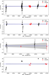 |
Fig. 1 TTVs with respect to linear ephemerides for TOI-5624 b, c, d, and e (top to bottom). The grey shaded area marks the 1σ uncertainty region of the linear ephemerides’ model. |
Planetary parameters derived from LC and RV analyses with the MCMCI code.
5.2 Searching for a fifth transiting planet
We looked for the putative fifth planet both in the available TESS data and in the RV time series. The only transit-like signal we could detect in the photometry is in Sector 22 at the epoch TExoFOP = 2 458 924.4 BJD, which appears on the ExoFOP webpage7 as well. To check whether this transit-like signal is indeed genuine, we further extracted its TESS LC from the Full Frame Image (FFI; Sullivan et al. 2015). Briefly, we utilised the PATHOS pipeline (Nardiello et al. 2019), which uses FFIs, empirical point spread functions (PSFs), and the Gaia DR3 catalogue, to extract the LCs of the target star with five different methods (PSF-fitting, 1-px, 2-px, 3-px, and 4-px radius aperture photometry) after subtracting all the neighbouring stars within a radius of 10 pixels (∼3.5′) from TOI-5624. Raw light curves were then corrected with co-trending basis vectors (Nardiello et al. 2021), to minimise the RMS and preserve the stellar variability (see Appendix A of Nardiello et al. 2025 for further details).
Although we were able to fit a transit model onto the PDC-SAP flux (Fig. B.1, left) with a depth of  ppm, two similar MCMCI analyses using the SAP and PATHOS-extracted fluxes led to no transit (no_tr) detections (Fig. B.1, middle and right). If we force a planet to transit within the SAP and PATHOS LCs (tr scenario) by fixing the planet parameters to those inferred from the PDCSAP analysis, run MCMCI, and compute ∆BIC = BICtr – BICno_tr, we get ∆BIC = +10 and +16 for the SAP and PATHOS photometry, respectively. As the outcomes depend on the photometric extraction pipelines, with the BIC that does not favour the transit scenario, we rejected the hypothesis that a fifth planet transits within the available photometry and we focussed on the RV time series.
5.3 Searching for a fifth planet in the RV data
We first computed the generalised Lomb-Scargle (GLS) periodograms (Zechmeister & Kürster 2009) of different RV-related activity indicators (see Sect. 3.1). As shown in Fig. B.2, there is always a prominent peak at ∼20 days, which is likely the rotation period of the star, Prot,*. This is consistent with the upper limit  = 20.7 ± 5.2 d, as inferred from Ri, and v sin i*; we note that Prot,* ∼ 20 d is close to the orbital period of TOI-5624 e. To corroborate our conclusions, for each of the five TESS sectors extracted by the SAP, we removed all the temporal windows containing transit events and we produced the corresponding GLS periodogram plus a second one after removing the most prominent peak from the first one (Fig. B.3). All these pairs of periodograms peak at Prot,* ∼ 20 d and at its first harmonic (Prot,*/2), except for Sector 75 whose most prominent peaks are the second (Prot,*/3) and first (Prot,*/2) harmonic of Prot,*.
We then performed an RV-only analysis by fitting the four transiting planets on circular orbits using the MCMCI code that allows the simultaneous detrending of the RV time series against time and four ancillary parameters via low-order polynomials. After executing several MCMCI mini-runs, where we alternated different combinations of four ancillary parameters extracted from the seven activity indicators available for the detrending of the SN-based HARPS-N data, it turned out that the set (FWHMSN, γ, NaD2, Hα) displays the best performance in removing the stellar activity, as quantified by the BIC. For SOPHIE data, instead, we used the RV-related activity indicators given by the official pipeline described in Sect. 3.2. Then, we launched two independent MCMCI runs and after checking the convergence of the jump parameters (i.e. the time of inferior conjunction, T0, the orbital period, P, and the RV semiamplitude, K) via the GR statistic (R̃ < 1.003), we computed the GLS periodogram of the HARPS-N RV residuals (obtained after subtracting the Keplerians of the four transiting planets to the detrended RV time series: Fig. B.4, top panel) that peaks at ∼6.4d. After removing this signal (Fig. B.4, bottom panel), the highest peak is at ∼45d followed by a peak at ∼10d. Fig. B.5 shows the pre-whitened GLS periodograms of the CCF FWHM (first row) and γ (second row) that peak at ∼10d and ∼6.4d. A similar behaviour is seen in the other RV-related activity indicators (not shown here). In addition, peaks at the same frequencies are found in the GLS periodograms of the SAP TESS LCs as mentioned above (Fig. B.3). Thus, we ascribed the ∼10d and ∼6.4d signals to the first and second harmonic of Prot,*, respectively. The signal at ∼45 d seen in Fig. B.4 has no counterpart in any of the activity indicators, hinting at the presence of an outer planet (TOI-5624 f). Planet f could be the perturber inducing the TTVs on TOI-5624 e, being their period ratio Pf : Pe close to the 2:1 first-order commensurability. We successfully explored the five-planet scenario in Sects. 5.4-5.6.
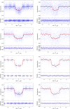 |
Fig. 2 Folded and detrendend LCs of planets b to e (top to bottom) as observed by CHEOPS (left) and TESS (right). Blue dots are the original data points, while black dots show the 20-minute binned data. The best-fit transit model is superimposed in red and the corresponding residuals are shown in the bottom panel of each plot. |
5.4 RV analysis with MCMCI: Five-planet fit
Using the MCMCI code, we modelled the HARPS-N RVs as extracted from the SN-fit (Sect. 3.1) and the SOPHIE RVs (Sect. 3.2) by fitting five planets on circular orbits, while imposing Gaussian priors on (P, T0) of the four transiting planets according to the linear ephemerides we derived in Section 5.1. The orbital period, Pf, and the time of inferior conjunction T0,f of TOI-5624 f as well as the RV semi-amplitudes of all the five planets were subject to uniform unbounded priors.
The stellar activity in the HARPS-N and SOPHIE time series ( and
and  , respectively) was simultaneously modelled within the MCMC framework via
![Mathematical equation: \begin{multlined} RV_{\star}^{\mathrm{HN}} = \beta_0^{\mathrm{HN}} + \beta_{1,t}^{\mathrm{HN}} t + \beta_{1,F}^{\mathrm{HN}} \mathrm{FWHM_{SN}} + \displaystyle\sum_{k=1}^{3}{\beta_{k,\gamma}^{\mathrm{HN}} \gamma^k}\\[-5pt] + \beta_{k,H\alpha}^{\mathrm{HN}} H\alpha + \displaystyle\sum_{k=1}^{3}{\beta_{k,\mathrm{NaD2}}^{\mathrm{HN}} \mathrm{NaD2}^k} - \beta_{\mathrm{h2}}\sin{\left[\frac{2\pi}{P_{\mathrm{h2}}}(t-T_{0,\mathrm{h2}})\right]}, \label{eq:RVactivityHN} \end{multlined}\nonumber \\](/articles/aa/full_html/2026/05/aa58740-25/aa58740-25-eq60.png) (1)
(1)
![Mathematical equation: \begin{multlined} RV_{\star}^{\mathrm{SO}} = \beta_0^{\mathrm{SO}} + \displaystyle\sum_{k=1}^{2}{\beta_{k,t}^{\mathrm{SO}} t^k} + \displaystyle\sum_{k=1}^{4}{\beta_{k,\mathrm{BIS}}^{\mathrm{SO}} \mathrm{BIS}^k} + \displaystyle\sum_{k=1}^{3}{\beta_{k,A}^{\mathrm{SO}} A^k} \\ + \displaystyle\sum_{k=1}^{4}{\beta_{k,R}^{\mathrm{SO}} \log{R'_{\mathrm{HK}}}^k} - \beta_{\mathrm{h2}}\sin{\left[\frac{2\pi}{P_{\mathrm{h2}}}(t-T_{0,\mathrm{h2}})\right]}, \label{eq:RVactivitySO} \end{multlined}](/articles/aa/full_html/2026/05/aa58740-25/aa58740-25-eq61.png) (2)
(2)
where the β parameters are the polynomial coefficients, the polynomial orders were assessed following the BIC minimisation criterion and the sinusoid’s parameters, Ph2 and T0,h2, were subject to the following Gaussian priors8 Ph2 = N(6.391,0.011) and T0,h2 = N(2 459 979.29,0.21) as inferred from the periodogram in Fig. B.4 that shows the second harmonic of Prot,*.
We performed four independent MCMCI runs made of 100 000 steps each (burn-in 20%) that consistently converged according to the GR statistic (R < 1.027). As listed in Table 2, we obtained robust mass estimates for TOI-5624 b, e, and f (detection >3 σ), while measuring the mass of TOI-5624 c and d at the 2.5 and 2.2σ level, respectively. We obtained Mb = 9.4 ± 1.4 M⊕, Mc = 4.8 ± 1.9 M⊕, Md = 4.9 ± 2.2 M⊕, Me =  M⊕ for planets b to e, and a planet minimum mass Mf sin if = 13.0 ± 3.7 M⊕ for TOI-5624 f. Each panel in Fig. 3 shows the detrended RV time series phase-folded to the period of that planet, after removing the Keplerian signals of the other planets detected in the system.
We further performed a similar MCMCI analysis, but allowing the planetary eccentricities to vary. For each planet, we assumed (e cos w; e sin ω) as jump parameters, where e is the orbital eccentricity and ω the argument of periastron (Anderson et al. 2011). It turned out that all the e values do not significantly differ from zero, being less than 1.5σ away from zero. In addition, when comparing the circular analysis (e = 0) with the eccentric one (e ≠ 0), we obtained ∆BIC = BICe≠0 – BICe=0 = +37, which states that assuming circular orbits is a reasonable assumption given the RV data in our hands. Moreover, the TTV dynamical analysis performed in Sect. 5.6 confirms low orbital eccentricities with e values that again do not significantly differ from zero. The eccentricity value exhibiting the maximum σ-deviation from zero (∼2.7σ) is ee =  (Sect. 5.6; Tab. C.5). Kipping (2008) shows that in low-eccentricity systems (e lower than a few hundredths), the transit light curve remains effectively indistinguishable from a circular orbit (e = 0) model, which justifies the assumption for e = 0 both in the RV analysis and in the photometric analysis of Sect. 5.1.
By propagating the coarse ephemerides of TOI-5624 f obtained from the RVs, there is a full sequence of epochs not covered by the available photometric data in which the planet could have transited its host star. While the RV data alone cannot rule out the hypothesis that TOI-5624 f is a transiting planet, the dynamical analysis (Sect. 5.6) finds TOI-5624f as a nontransiting planet. Future photometric surveys may help clarify this, though TESS is not currently foreseen to re-observe this system9.
Finally, we note that all the transiting planets are consistent with being coplanar given their orbital inclinations i (see Table 2). By combining a/R* of TOI-5624 f and that the planet does not transit, we inferred an orbital inclination if < 89°, which differs at least by ∼ 0.5° from the average orbital inclination of the transiting planets in the system. On the one hand, this difference may be small if compared with the typical mutual inclination dispersion among Kepler (Borucki et al. 2010) multi-planet systems, which amounts to a few degrees (see e.g. Millholland et al. 2021, and references therein). On the other hand, this difference is large with respect to the standard deviation of 0.12° as computed from the orbital inclinations of the planets transiting TOI-5624, which might challenge the present-day dynamical models in the interpretation of the system architecture.
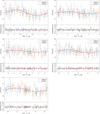 |
Fig. 3 Detrended RV time series folded according to the period of TOI-5624b (top-left), TOI-5624c (top-right), TOI-5624d (middleleft), TOI-5624e (middle-right), and TOI-5624f (bottom-left) after removing the Keplerian signals of the other planets as inferred from the MCMCI analysis. The marker colour distinguishes the two different instruments (light blue for HARPS-N and orange for SOPHIE), while the red line represents the inferred model. The jitter contribution in the error bars is highlighted in grey. The RV semi-amplitudes are measured at the 6.9, 2.5, 2.2, 3.1, and 3.5σ level for planets b, c, d, e, and f, respectively. |
5.5 RV analysis with pyaneti
As a sanity check, we jointly modelled the HARPS-N TERRA RVs and activity indicators following a multi-dimensional GP approach (Rajpaul et al. 2015) as implemented in the MCMC-based code pyaneti (Barragán et al. 2019, 2022). This approach assumes that the same function G(t) and its time derivative Ġ(t) can describe the activity-induced stellar signal seen both in the Doppler measurements and in the activity indicators. For this purpose, alongside the RVs, we modelled the FWHM of the DRS cross-correlation functions, as its periodogram shows a strong signal at the stellar rotation period (Prot,* ≈ 20d). Following Rajpaul et al. (2015), we used a 2D GP defined as
 (3a)
(3a)
 (3b)
(3b)
where ARV and AFWHM are offset terms, while BRV, CRV, and BFWHM are amplitudes that relate the function G(t) and G(t) to the RV and FWHM time series. For the GP, we chose the following quasi-periodic covariance function,
![Mathematical equation: \kappa(t_{i},t_{j}) = \exp\left[- \frac{\sin{^2}\left[\pi(t_{i}-t_{j})/P_\mathrm{GP}\right]}{2\lambda_\mathrm{p}^{2}} - \frac{(t_{i}-t_{j})^{2}}{2\lambda_\mathrm{e}^{2}}\right]\,,](/articles/aa/full_html/2026/05/aa58740-25/aa58740-25-eq66.png) (4)
(4)
where PGP is the characteristic period of the GP (interpreted as Prot,*), λp is the inverse of the harmonic complexity (accounting for the distribution of active regions on the stellar surface), and λe is the long-term evolution timescale of spots and plages.
To account for the Doppler reflex motions induced by the five planets orbiting TOI-5624, we added five Keplerians to the RV model in Eq. (3a). We assumed the orbits to be circular and adopted Gaussian priors on periods (P) and times of reference transit (T0) for the four transiting planets (TOI-5624 b, c, d, and e), as derived from the modelling presented in Sect. 5.1. RV and FWHM jitter terms were also modelled to account for any instrumental noise that was not already captured in the nominal uncertainties. We used uniform priors for the orbital period and time of inferior conjunction of the non-transiting outer planet (TOI-5624 f), as well as for the RV semi-amplitudes of all five planets (Table C.4). For the GP parameters, we adopted a uniform prior on PGP centred on the stellar rotation period found by the frequency analysis of the activity indicators, and wide uniform priors for the remaining hyperparameters and amplitudes, as listed in Table C.4. We sampled the parameter space with 500 chains and used the last 500 iterations of the converged chains, applying a thin factor of 10 to obtain a final sample of 250 000 independent points for each fitted parameter.
Table C.4 reports the inferred values and uncertainties for both the model and the derived planetary parameters. They are defined as the median and 68.3% region of the credible interval of the marginalised posterior distributions for each inferred parameter. The time series of the HARPS-N TERRA Doppler measurements and FWHM of the DRS cross-correlation functions are shown in Fig. B.6, along with the inferred models, and the phase-folded Doppler reflex motions induced by each planet. We found that multi-dimensional GP-derived RV variations are in excellent agreement (within 1σ) with those presented in Sect. 5.4, corroborating our results.
5.6 TTV+RV dynamical analysis
As shown in Figure 1, TOI-5624 e exhibits significant TTVs, indicative of strong gravitational interactions within the system. These variations could be driven by both the neighbouring planet d, which lies close to a 3:2 commensurability with planet e, and by a possible outer non-transiting companion, planet f, whose signal is detected in the radial velocities and appears near a 2:1 commensurability with planet e.
To investigate the dynamical origin of the observed TTVs and to test the plausibility of the fifth planet, we performed a joint N-body analysis of the system using the TRAnsits and Dynamics of Exoplanetary Systems (TRADES, Borsato et al. 2014, 2019, 2021, 2024)10 code. This allowed us to integrate the full N-body equations of motion and to simultaneously fit both transit times and the detrended radial velocities taken from Tables A.1 and A.2. The analysis was carried out under two different hypotheses: (1) a four-planet system including only the transiting planets (from b to e) and (2) a five-planet configuration including an additional planet f.
Given the extensive integration time required (five years) to reproduce the observational baseline and the short orbital periods of the two inner planets (b and c), we neglected their mutual gravitational interactions in the N -body model. This simplification is justified because the inner planets lie far from first-order resonances with the outer planet and, therefore, they are expected to have a negligible dynamical influence on its TTVs. The period ratio Pd/Pc = 1.742 places the pair ∼0.5% interior to the 7:4 commensurability, while Pd/Pb = 4.05 lies ∼1.3% exterior to the 4:1 commensurability. Both correspond to higher order resonances, which are expected to generate substantially weaker TTV signals compared to first-order resonances, as their strength scales with higher powers of the orbital eccentricity and therefore becomes negligible for near-circular orbits (e.g. Murray & Dermott 1999; Agol & Deck 2016). This interpretation is further supported by Fig. 1, where the two inner planets do not show significant deviations from a linear ephemeris.
For each planet, we fit the orbital period P, the planet-to-star mass ratio, Mp/M*, the eccentricity, e, the argument of periastron, ω, and the mean longitude, λ11. To reduce correlations and improve sampling efficiency, we employed the parametrisation (√e cos ω, √e sin ω) instead of fitting e and ω directly (Anderson et al. 2011). The stellar parameters (M*, R*) and the planetary radii (Rp), together with the orbital inclinations, i, were fixed to the values reported in Tables 1 and 2. The longitude of the ascending node was set to Ω = 180° for planet d and e. For the outer planet f, both the orbital inclination and the longitude of the ascending node were left as free parameters, with Ωf sampled uniformly within [170°, 190°] to explore possible small mutual inclinations with the inner system. We adopted uniform priors on all fitted parameters (see Table C.5) and included an additional RV jitter term, σjitter, parametrised as log2 σjitter to ensure efficient sampling.
The exploration of the parameter space was initially performed using the PyDE12 differential evolution optimiser (Storn & Price 1997; Parviainen et al. 2016), with a population of 120 individuals evolved over 100000 generations. The best-fitting solutions from this stage were adopted as starting points for the emcee ensemble sampler (Foreman-Mackey et al. 2013), which employed 120 walkers to explore the posterior distribution for 500 000 steps. Following the approach of Leonardi et al. (2025), the emcee sampling combined two proposal schemes: a differential evolution proposal for 80% of the walkers (Nelson et al. 2014) and a snooker update for the remaining 20% (ter Braak & Vrugt 2008), improving mixing efficiency in multi-modal posteriors. Convergence of the chains was assessed using the Geweke (Geweke 1991) and GR diagnostics, together with autocorrelation analysis (Goodman & Weare 2010) and visual inspection, requiring the total chain length to exceed 50 integrated autocorrelation times. The first 250 000 steps were discarded as burn-in, and the chains were thinned by a factor of 100.
The final parameter estimates along with the adopted priors are listed in Table C.5. The observed-minus-calculated (O–C) diagrams for hypotheses (1) and (2) are shown in Figs. B.7 and 4, respectively. The fit to the transit timings of TOI-5624 e is noticeably poorer under the four-planet configuration. Indeed, model comparison between the four-planet (4p) and five-planet (5p) scenarios was performed via ∆BIC = BIC5p – BIC4p. The resulting value, ∆BIC = –80, strongly favours the inclusion of the fifth outer planet TOI-5624 f. Likewise, adopting the approximate relation for the logarithm of the Bayes factor,  (Kass & Raftery 1995), we obtained log B = +40, which further confirms an increased evidence for the five-planet configuration. While the five-planet model reproduces the overall timing pattern of TOI-5624 d and e (see Fig. 4), the resulting posterior distributions do not yield significant improvements in the planetary mass estimates with respect to the RV-only analyses. In particular, the inclination of the outer planet f remains largely unconstrained and tends to favour a non-coplanar, non-transiting configuration. The orbital period of TOI-5624 f turned out to be Pf,dyn =
  d that differs from the strict Pf :Pe = 2:1 commensurability by 2.6%. It is consistent with the estimate from the RV analysis (Pf,RV =
  d) at the ∼1.4σ level.
To further assess the robustness of the five-planet solution, we performed two additional dynamical analyses. First, we re-ran the TTV+RV analysis adopting a broader prior on the orbital period of the outer planet, allowing Pf to vary within the interval [1,50] days. This range also includes configurations in which the additional planet would reside between TOI-5624 d and TOI-5624 e. Second, we repeated the dynamical fit using only the transit mid-times (Ttr), excluding the RV measurements, but leaving the broader prior on the period of planet f. This test was designed to verify that the inferred signal of the fifth planet is not driven primarily by the RV dataset, where the Keplerian reflex motion associated with TOI-5624 f is clearly detected. Both tests yield results consistent with the nominal five-planet solution (see Fig. B.8), recovering a planetary signal with orbital periods of  and
and  days, respectively. These sanity checks support the robustness of the inferred architecture and indicate that the detection of TOI-5624 f is not sensitive to the adopted prior assumptions or to the inclusion of the RV dataset. In other words, only an outer perturber is capable of reproducing the observed TTVs of planet e.
Following Correia et al. (2005, 2010), we also ran a stability analysis of the best-fit solution (Table 2). The system was integrated over 104 yr for each initial condition and a stability indicator was calculated from the frequency analysis of the mean longitude (Laskar 1990, 1993) of TOI-5624 f. We found that the five-planet system is stable, the strict 2:1 MMR between TOI-5624 e and f would be unstable, except for a small stability region around P ~ 42.9 day and eccentricities lower than 0.01, with planet f that is not trapped in there in any case (Fig. B.9, left panel). We also found that the inclination of TOI-5624 f must be around 90° ± 60° (Fig. B.9, right panel); thus, we can put an upper limit on its true mass  .
.
Given the current temporal baseline and the limited sampling of the expected TTV super-period, the available data do not allow for a robust dynamical mass determination. Additional (e.g. CHEOPS) transit observations, ideally spanning a longer temporal window, are therefore required to better sample the TTV modulation, to reduce the degeneracies between mass and eccentricity, and to confirm the dynamical link between TOI-5624 e and f. In the perspective of follow-up observations, we note that future transit timings of TOI-5624 d predicted by the dynamical model are consistent with the linear ephemeris reported in Table 2. In case of TOI-5624 e, instead, the uncertainties of the predicted transit timings would not aid with the scheduling of future transit events. Thus, we suggest to account for a ∼1.5h buffer (i.e. the peak-to-peak amplitude of the observed TTVs) when planning future observations of TOI-5624 e.
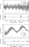 |
Fig. 4 O–C diagrams of TOI-5624 d (top) & e (bottom) along with the residuals (res) with respect to the best-fit model when assuming the five-planet configuration. The best-fit TRADES model is shown as a black line, while the shaded areas display the 1σ, 2σ, and 3σ confidence intervals. |
6 Conclusions
TOI-5624 hosts four transiting sub-Neptunes (orbital periods Pb ≈ 3.4, Pc ≈ 7.9, Pd ≈ 13.7, and Pe ≈ 21.5 days; Rp: 2.3-3.6R⊕) that we characterised using TESS and CHEOPS photometry. The outermost planet (i.e. TOI-5624 e) is affected by statistically significant TTVs (∼80 min peak-to-peak). We thus searched for additional planets in the system that could explain the observed TTV pattern, but found none in the available photometry. We then conducted frequency analyses of the HARPS-N RV time series and found a signal hinting at the presence of an outer planet near a 2:1 period commensurability with TOI-5624 e. Thus, we performed two fully independent RV analyses (both in terms of the extraction technique for retrieving the RV time series and of the MCMC statistical framework employed for the data analysis) in which we assumed a five-planet scenario. All jump parameters converged and the two independent analyses gave consistent results within 1σ, obtaining Mb = 9.4 ± 1.4 M⊕ (ρb =  gcm−3), Mc = 4.8 ± 1.9 M⊕ (ρc =
  gcm−3), Md = 4.9 ± 2.2 M⊕ (ρd =
  g cm−3), Me =
  M⊕ (ρe = 1.46 ± 0.48 g cm−3) for planets b to e, and a planet minimum mass Mf sin if = 13.0 ± 3.7 M⊕ for TOI-5624 f. Stability simulations suggest a mass upper limit
  for this outer planet.
We finally investigated the dynamical origin of the TTV pattern exhibited by TOI-5624 e by performing two N-body analyses of the system considering either a four or a five-planet configuration. We found that the five-planet scenario is much more favoured by the Bayesian evidence (∆BIC = –78) and that the model is able to properly reproduce the transit times’ pattern observed for TOI-5624 e. This constitutes an independent confirmation of TOI-5624 f. However, further photometric observations are required to properly map the phase of the TTV super period, to dynamically constrain the planet masses, and to definitely confirm the dynamical link between TOI-5624 e and f.
Hosting at least five planets, TOI-5624 is a golden target in the context of multi-planet systems and we were able to characterise the radii of the four transiting planets at a precision level better than ∼1.7%, while firmly detecting three planets in the RV time series (precision >3σ). The RV semi-amplitudes of the other two planets (i.e. TOI-5624 c and d) were measured at the 2.5 and 2.2σ level, respectively. As of today13, 76 multi-planet systems containing at least four transiting planets are known out of the ∼4500 validated exoplanet systems. Of these, only four systems, namely, TRAPPIST-1 (Agol et al. 2021), HD110067 (Luque et al. 2023), TOI-178 (Leleu et al. 2024), and HIP41378 (Howard et al. 2025), have been characterised well enough to measure the radii of at least four of their planets with a precision better than 2%. Moreover, TOI-5624 is the only system for which at least three planet masses were firmly measured (>3σ) using RV data only. Future photometric and RV data would enable the investigation of the presence of additional planets, making this system an even more compelling subject of study.
Data availability
The full Tables A.1 & A.2 and detrended CHEOPS light curves are available at the CDS via https://cdsarc.cds.unistra.fr/viz-bin/cat/J/A+A/709/A265.
Acknowledgements
We thank the anonymous referee, as the comments provided have sensibly improved the quality of the manuscript. CHEOPS is an ESA mission in partnership with Switzerland with important contributions to the payload and the ground segment from Austria, Belgium, France, Germany, Hungary, Italy, Portugal, Spain, Sweden, and the United Kingdom. The CHEOPS Consortium would like to gratefully acknowledge the support received by all the agencies, offices, universities, and industries involved. Their flexibility and willingness to explore new approaches were essential to the success of this mission. CHEOPS data analysed in this article will be made available in the CHEOPS mission archive (https://cheops.unige.ch/archive_browser/). D.Ga. and L.M.Se. acknowledge financial support from the CRT foundation under Grant No. 2018.2323 ‘Gaseous or rocky? Unveiling the nature of small worlds’. C.Br. and A.Si. acknowledge support from the Swiss Space Office through the ESA PRODEX program. S.G.S. acknowledge support from FCT through FCT contract nr. CEECIND/00826/2018 and POPH/FSE (EC). The Portuguese team thanks the Portuguese Space Agency for the provision of financial support in the framework of the PRODEX Programme of the European Space Agency (ESA) under contract number 4000142255. T.Wi. acknowledges support from the UKSA and the University of Warwick. A.Co., A.De., B.Ed., K.Ga., and J.Ko. acknowledge their role as ESA-appointed CHEOPS Science Team Members. A.Br. was supported by the SNSA. M.G. is F.R.S.-FNRS Research Director. BAk and MLe acknowledge support of the Swiss National Science Foundation under grant number PCEFP2_194576. Y.Al. acknowledges support from the Swiss National Science Foundation (SNSF) under grant 200020_192038. R.Al., D.Ba., E.Pa., I.Ri., and E.Vi. acknowledge financial support from the Agencia Estatal de Investigación of the Ministerio de Ciencia e Innovación MCIN/AEI/10.13039/501100011033 and the ERDF “A way of making Europe” through projects PID2021-125627OB-C31, PID2021-125627OB-C32, PID2021-127289NB-I00, PID2023-150468NB-I00 and PID2023-149439NB-C41. S.C.C.B. acknowledges the support from Fundação para a Ciência e Tecnologia (FCT) in the form of work contract through the Scientific Employment Incentive program with reference 2023.06687.CEECIND and DOI 10.54499/2023.06687.CEECIND/CP2839/CT0002. L.Bo., V.Na., IPa., G.Pi., R.Ra., G.Sc., and T.Zi. acknowledge support from CHEOPS ASI-INAF agreement n. 2019-29-HH.0. T.Zi. also acknowledges support from NVIDIA Academic Hardware Grant Program for the use of the Titan V GPU card and the Italian MUR Departments of Excellence grant 2023-2027 “Quantum Frontiers”. A.C.C. acknowledges support from STFC consolidated grant number ST/V000861/1, and UKSA grant number ST/X002217/1. P.E.C. is funded by the Austrian Science Fund (FWF) Erwin Schroedinger Fellowship, program J4595-N. This project was supported by the CNES. A.De. acknowledges financial support from the Swiss National Science Foundation (SNSF) for project 200021_200726. This work was supported by FCT - Fundaçâo para a Ciência e a Tecnologia through national funds and by FEDER through COM-PETE2020 through the research grants UIDB/04434/2020, UIDP/04434/2020, 2022.06962.PTDC. O.D.S.D. is supported in the form of work contract (DL 57/2016/CP1364/CT0004) funded by national funds through FCT. B.-O.D. acknowledges support from the Swiss State Secretariat for Education, Research and Innovation (SERI) under contract number MB22.00046. This project has received funding from the Swiss National Science Foundation for project 200021_200726. It has also been carried out within the framework of the National Centre of Competence in Research PlanetS supported by the Swiss National Science Foundation under grants 51NF40_182901 and 51NF40_205606. The authors acknowledge the financial support of the SNSF. M.F. and C.M.P. gratefully acknowledge the support of the Swedish National Space Agency (DNR 65/19, 174/18). M.N.G. is the ESA CHEOPS Project Scientist and Mission Representative. B.M.M. is the ESA CHEOPS Project Scientist. KGI was the ESA CHEOPS Project Scientist until the end of December 2022 and Mission Representative until the end of January 2023. All of them are/were responsible for the Guest Observers (GO) Programme. None of them relay/relayed proprietary information between the GO and Guaranteed Time Observation (GTO) Programmes, nor do/did they decide on the definition and target selection of the GTO Programme. CHe acknowledges financial support from the Österreichische Akademie der Wissenschaften and from the European Union H2020-MSCA-ITN-2019 under Grant Agreement no. 860470 (CHAMELEON). Calculations were performed using supercomputer resources provided by the Vienna Scientific Cluster (VSC). K.W.F.L. was supported by Deutsche Forschungsgemeinschaft grants RA714/14-1 within the DFG Schwerpunkt SPP 1992, Exploring the Diversity of Extrasolar Planets. This work was granted access to the HPC resources of MesoPSL financed by the Region Ile de France and the project Equip@Meso (reference ANR-10-EQPX-29-01) of the programme Investissements d’Avenir supervised by the Agence Nationale pour la Recherche. P.M. acknowledges support from STFC research grant number ST/R00063 8/1. This work was also partially supported by a grant from the Simons Foundation (PI: Queloz, grant number 327127). N.C.Sa. acknowledges funding by the European Union (ERC, FIERCE, 101052347). Views and opinions expressed are however those of the author(s) only and do not necessarily reflect those of the European Union or the European Research Council. Neither the European Union nor the granting authority can be held responsible for them. Gy.M.Sz. acknowledges the support of the Hungarian National Research, Development and Innovation Office (NKFIH) grant K-125015, a PRODEX Experiment Agreement No. 4000137122, the Lendület LP2018-7/2021 grant of the Hungarian Academy of Science and the support of the city of Szombathely. V.V.G. is an F.R.S-FNRS Research Associate. JV acknowledges support from the Swiss National Science Foundation (SNSF) under grant PZ00P2_208945. NAW acknowledges UKSA grant ST/R004838/1. This work uses observations secured with the SOPHIE spectrograph at the 1.93-m telescope of Observatoire Haute-Provence, France, with the support of its staff. This work was supported by the “Programme National de Planétologie” (PNP) of CNRS/INSU, and CNES. The stability maps were performed at the Oblivion Supercomputer at the University of Évora (https://oblivion.hpc.uevora.pt).
References
- Agol, E., & Deck, K. 2016, ApJ, 818, 177 [Google Scholar]
- Agol, E., & Fabrycky, D. C. 2018, in Handbook of Exoplanets, eds. H. J. Deeg, & J. A. Belmonte (Cambridge: Cambridge University Press), 7 [Google Scholar]
- Agol, E., Steffen, J., Sari, R., & Clarkson, W. 2005, MNRAS, 359, 567 [Google Scholar]
- Agol, E., Dorn, C., Grimm, S. L., et al. 2021, Planet. Sci. J., 2, 1 [NASA ADS] [CrossRef] [Google Scholar]
- Alibert, Y., Carron, F., Fortier, A., et al. 2013, A&A, 558, A109 [NASA ADS] [CrossRef] [EDP Sciences] [Google Scholar]
- Anderson, D. R., Smith, A. M. S., Lanotte, A. A., et al. 2011, MNRAS, 416, 2108 [NASA ADS] [CrossRef] [Google Scholar]
- Anglada-Escudé, G., & Butler, R. P. 2012, ApJS, 200, 15 [Google Scholar]
- Armitage, P. J. 2024, arXiv e-prints [arXiv:2412.11064] [Google Scholar]
- Baranne, A., Queloz, D., Mayor, M., et al. 1996, A&AS, 119, 373 [Google Scholar]
- Barragán, O., Gandolfi, D., & Antoniciello, G. 2019, MNRAS, 482, 1017 [Google Scholar]
- Barragán, O., Aigrain, S., Rajpaul, V. M., & Zicher, N. 2022, MNRAS, 509, 866 [Google Scholar]
- Benz, W., Broeg, C., Fortier, A., et al. 2021, Exp. Astron., 51, 109 [Google Scholar]
- Blackwell, D. E., & Shallis, M. J. 1977, MNRAS, 180, 177 [NASA ADS] [CrossRef] [Google Scholar]
- Boisse, I., Eggenberger, A., Santos, N. C., et al. 2010, A&A, 523, A88 [NASA ADS] [CrossRef] [EDP Sciences] [Google Scholar]
- Bonfanti, A., & Gillon, M. 2020, A&A, 635, A6 [NASA ADS] [CrossRef] [EDP Sciences] [Google Scholar]
- Bonfanti, A., Ortolani, S., Piotto, G., & Nascimbeni, V. 2015, A&A, 575, A18 [NASA ADS] [CrossRef] [EDP Sciences] [Google Scholar]
- Bonfanti, A., Ortolani, S., & Nascimbeni, V. 2016, A&A, 585, A5 [NASA ADS] [CrossRef] [EDP Sciences] [Google Scholar]
- Bonfanti, A., Delrez, L., Hooton, M. J., et al. 2021, A&A, 646, A157 [EDP Sciences] [Google Scholar]
- Bonfanti, A., Gandolfi, D., Egger, J. A., et al. 2023, A&A, 671, L8 [NASA ADS] [CrossRef] [EDP Sciences] [Google Scholar]
- Bonfanti, A., Amateis, I., Gandolfi, D., et al. 2025, A&A, 693, A90 [NASA ADS] [CrossRef] [EDP Sciences] [Google Scholar]
- Borsato, L., Marzari, F., Nascimbeni, V., et al. 2014, A&A, 571, A38 [NASA ADS] [CrossRef] [EDP Sciences] [Google Scholar]
- Borsato, L., Malavolta, L., Piotto, G., et al. 2019, MNRAS, 484, 3233 [NASA ADS] [CrossRef] [Google Scholar]
- Borsato, L., Degen, D., Leleu, A., et al. 2024, A&A, 689, A52 [NASA ADS] [CrossRef] [EDP Sciences] [Google Scholar]
- Borsato, L., Piotto, G., Gandolfi, D., et al. 2021, MNRAS, 506, 3810 [NASA ADS] [CrossRef] [Google Scholar]
- Borucki, W. J., Koch, D., Basri, G., et al. 2010, Science, 327, 977 [Google Scholar]
- Bouchy, F., Hébrard, G., Udry, S., et al. 2009, A&A, 505, 853 [NASA ADS] [CrossRef] [EDP Sciences] [Google Scholar]
- Bouchy, F., Díaz, R. F., Hébrard, G., et al. 2013, A&A, 549, A49 [NASA ADS] [CrossRef] [EDP Sciences] [Google Scholar]
- Castelli, F., & Kurucz, R. L. 2003, IAU Symp., 210, A20 [Google Scholar]
- Correia, A. C. M., Udry, S., Mayor, M., et al. 2005, A&A, 440, 751 [NASA ADS] [CrossRef] [EDP Sciences] [Google Scholar]
- Correia, A. C. M., Couetdic, J., Laskar, J., et al. 2010, A&A, 511, A21 [NASA ADS] [CrossRef] [EDP Sciences] [Google Scholar]
- Correia, A. C. M., Delisle, J.-B., & Laskar, J. 2018, in Handbook of Exoplanets, eds. H. J. Deeg, & J. A. Belmonte (Berlin: Springer International Publishing AG, part of Springer Nature), 12 [Google Scholar]
- Cosentino, R., Lovis, C., Pepe, F., et al. 2012, SPIE Conf. Ser., 8446, 84461V [Google Scholar]
- Deck, K. M., & Agol, E. 2015, ApJ, 802, 116 [NASA ADS] [CrossRef] [Google Scholar]
- Egger, J. A., Osborn, H. P., Kubyshkina, D., et al. 2024, A&A, 688, A223 [NASA ADS] [CrossRef] [EDP Sciences] [Google Scholar]
- Espinoza, N., & Jordán, A. 2015, MNRAS, 450, 1879 [Google Scholar]
- Fausnaugh, M., Huang, X., Glidden, A., Guerrero, N., & TESS Science Office. 2018, AAS Meeting Abs., 231, 439.09 [Google Scholar]
- Foreman-Mackey, D., Hogg, D. W., Lang, D., & Goodman, J. 2013, PASP, 125, 306 [Google Scholar]
- Foreman-Mackey, D., Agol, E., Ambikasaran, S., & Angus, R. 2017, AJ, 154, 220 [Google Scholar]
- Fortier, A., Alibert, Y., Carron, F., Benz, W., & Dittkrist, K. M. 2013, A&A, 549, A44 [NASA ADS] [CrossRef] [EDP Sciences] [Google Scholar]
- Fortier, A., Simon, A. E., Broeg, C., et al. 2024, A&A, 687, A302 [NASA ADS] [CrossRef] [EDP Sciences] [Google Scholar]
- Gaia Collaboration (Vallenari, A., et al.) 2023, A&A, 674, A1 [NASA ADS] [CrossRef] [EDP Sciences] [Google Scholar]
- Gelman, A., & Rubin, D. B. 1992, Stat. Sci., 7, 457 [Google Scholar]
- Geweke, J. F. 1991, Evaluating the accuracy of sampling-based approaches to the calculation of posterior moments, Staff Report 148, Federal Reserve Bank of Minneapolis [Google Scholar]
- Goldreich, P., & Tremaine, S. 1980, ApJ, 241, 425 [Google Scholar]
- Goodman, J., & Weare, J. 2010, Commun. Appl. Math. Comput. Sci., 5, 65 [Google Scholar]
- Hadden, S., & Lithwick, Y. 2017, AJ, 154, 5 [Google Scholar]
- Haldemann, J., Dorn, C., Venturini, J., Alibert, Y., & Benz, W. 2024, A&A, 681, A96 [NASA ADS] [CrossRef] [EDP Sciences] [Google Scholar]
- Hatzes, A. P. 2019, The Doppler Method for the Detection of Exoplanets (Oxford: IOP Publishing), 2514 [Google Scholar]
- Heidari, N., Boisse, I., Hara, N. C., et al. 2024, A&A, 681, A55 [NASA ADS] [CrossRef] [EDP Sciences] [Google Scholar]
- Heidari, N., Hébrard, G., Martioli, E., et al. 2025, A&A, 694, A36 [NASA ADS] [CrossRef] [EDP Sciences] [Google Scholar]
- Henry, T. J., Soderblom, D. R., Donahue, R. A., & Baliunas, S. L. 1996, AJ, 111, 439 [Google Scholar]
- Hippke, M., & Heller, R. 2019, A&A, 623, A39 [NASA ADS] [CrossRef] [EDP Sciences] [Google Scholar]
- Hojjatpanah, S., Oshagh, M., Figueira, P., et al. 2020, A&A, 639, A35 [NASA ADS] [CrossRef] [EDP Sciences] [Google Scholar]
- Howard, A. W., Sinukoff, E., Blunt, S., et al. 2025, ApJS, 278, 52 [Google Scholar]
- Hoyer, S., Guterman, P., Demangeon, O., et al. 2020, A&A, 635, A24 [NASA ADS] [CrossRef] [EDP Sciences] [Google Scholar]
- Jenkins, J. M., Twicken, J. D., McCauliff, S., et al. 2016, SPIE Conf. Ser., 9913, 99133E [Google Scholar]
- Johansen, A., Ida, S., & Brasser, R. 2019, A&A, 622, A202 [NASA ADS] [CrossRef] [EDP Sciences] [Google Scholar]
- Kass, R. E., & Raftery, A. E. 1995, J. Am. Stat. Assoc., 90, 773 [Google Scholar]
- Khorshid, N., Min, M., Désert, J. M., Woitke, P., & Dominik, C. 2022, A&A, 667, A147 [NASA ADS] [CrossRef] [EDP Sciences] [Google Scholar]
- Kipping, D. M. 2008, MNRAS, 389, 1383 [NASA ADS] [CrossRef] [Google Scholar]
- Kurucz, R. L. 1993, SYNTHE Spectrum Synthesis Programs and Line Data (Cambridge, Mass.: Smithsonian Astrophysical Observatory) [Google Scholar]
- Laskar, J. 1990, Icarus, 88, 266 [NASA ADS] [CrossRef] [Google Scholar]
- Laskar, J. 1993, Phys. D Nonlinear Phenom., 67, 257 [Google Scholar]
- Lee, M. H., & Peale, S. J. 2002, arXiv e-prints [arXiv:0209176] [Google Scholar]
- Leleu, A., Alibert, Y., Hara, N. C., et al. 2021, A&A, 649, A26 [NASA ADS] [CrossRef] [EDP Sciences] [Google Scholar]
- Leleu, A., Delisle, J. B., Udry, S., et al. 2023, A&A, 669, A117 [NASA ADS] [CrossRef] [EDP Sciences] [Google Scholar]
- Leleu, A., Delisle, J.-B., Delrez, L., et al. 2024, A&A, 688, A211 [NASA ADS] [CrossRef] [EDP Sciences] [Google Scholar]
- Leonardi, P., Borsato, L., Pagliaro, L., et al. 2025, A&A, 702, A211 [NASA ADS] [CrossRef] [EDP Sciences] [Google Scholar]
- Lindegren, L., Bastian, U., Biermann, M., et al. 2021, A&A, 649, A4 [EDP Sciences] [Google Scholar]
- Lithwick, Y., Xie, J., & Wu, Y. 2012, ApJ, 761, 122 [Google Scholar]
- Lovis, C., & Pepe, F. 2007, A&A, 468, 1115 [NASA ADS] [CrossRef] [EDP Sciences] [Google Scholar]
- Luque, R., Osborn, H. P., Leleu, A., et al. 2023, Nature, 623, 932 [NASA ADS] [CrossRef] [Google Scholar]
- Malhotra, R. 1995, AJ, 110, 420 [NASA ADS] [CrossRef] [Google Scholar]
- Mandell, A. M. 2011, Planetary Migration (Berlin, Heidelberg: Springer Berlin Heidelberg), 1275 [Google Scholar]
- Marigo, P., Girardi, L., Bressan, A., et al. 2017, ApJ, 835, 77 [Google Scholar]
- Millholland, S. C., He, M. Y., Ford, E. B., et al. 2021, AJ, 162, 166 [Google Scholar]
- Mishra, L., Alibert, Y., Udry, S., & Mordasini, C. 2023, A&A, 670, A68 [NASA ADS] [CrossRef] [EDP Sciences] [Google Scholar]
- Munavar Hussain, M. J., & Kunimoto, M. 2025, AJ, 169, 91 [Google Scholar]
- Murray, C. D., & Dermott, S. F. 1999, Solar System Dynamics (Cambridge: Cambridge University Press) [Google Scholar]
- Nardiello, D., Borsato, L., Piotto, G., et al. 2019, MNRAS, 490, 3806 [NASA ADS] [CrossRef] [Google Scholar]
- Nardiello, D., Deleuil, M., Mantovan, G., et al. 2021, MNRAS, 505, 3767 [NASA ADS] [CrossRef] [Google Scholar]
- Nardiello, D., Akana Murphy, J. M., Spinelli, R., et al. 2025, A&A, 693, A32 [NASA ADS] [CrossRef] [EDP Sciences] [Google Scholar]
- Nelson, B., Ford, E. B., & Payne, M. J. 2014, ApJS, 210, 11 [Google Scholar]
- Osborn, H. P., Bonfanti, A., Gandolfi, D., et al. 2022, A&A, 664, A156 [NASA ADS] [CrossRef] [EDP Sciences] [Google Scholar]
- Parviainen, H., Pallé, E., Nortmann, L., et al. 2016, A&A, 585, A114 [NASA ADS] [CrossRef] [EDP Sciences] [Google Scholar]
- Pepe, F., Mayor, M., Galland, F., et al. 2002, A&A, 388, 632 [NASA ADS] [CrossRef] [EDP Sciences] [Google Scholar]
- Perruchot, S., Kohler, D., Bouchy, F., et al. 2008, SPIE Conf. Ser., 7014, 70140J [Google Scholar]
- Pont, F., Zucker, S., & Queloz, D. 2006, MNRAS, 373, 231 [NASA ADS] [CrossRef] [Google Scholar]
- Rajpaul, V., Aigrain, S., Osborne, M. A., Reece, S., & Roberts, S. 2015, MNRAS, 452, 2269 [Google Scholar]
- Rasmussen, C. E., & Williams, C. K. I. 2005, Gaussian Processes for Machine Learning, (Adaptive Computation and Machine Learning) (Cambridge: The MIT Press) [Google Scholar]
- Raymond, S. N., & Morbidelli, A. 2022, Planet Formation: Key Mechanisms and Global Models (Cham: Springer International Publishing), 3 [Google Scholar]
- Ricker, G. R., Winn, J. N., Vanderspek, R., et al. 2015, J. Astron. Teles. Instrum. Syst., 1, 014003 [Google Scholar]
- Salmon, S. J. A. J., Van Grootel, V., Buldgen, G., Dupret, M. A., & Eggenberger, P. 2021, A&A, 646, A7 [NASA ADS] [CrossRef] [EDP Sciences] [Google Scholar]
- Santos, N. C., Sousa, S. G., Mortier, A., et al. 2013, A&A, 556, A150 [NASA ADS] [CrossRef] [EDP Sciences] [Google Scholar]
- Schanche, N., Hébrard, G., Collier Cameron, A., et al. 2020, MNRAS, 499, 428 [NASA ADS] [CrossRef] [Google Scholar]
- Schwarz, G. 1978, Ann. Stat., 6, 461 [Google Scholar]
- Scuflaire, R., Théado, S., Montalbán, J., et al. 2008, Ap&SS, 316, 83 [Google Scholar]
- Simola, U., Dumusque, X., & Cisewski-Kehe, J. 2019, A&A, 622, A131 [NASA ADS] [CrossRef] [EDP Sciences] [Google Scholar]
- Skrutskie, M. F., Cutri, R. M., Stiening, R., et al. 2006, AJ, 131, 1163 [NASA ADS] [CrossRef] [Google Scholar]
- Smith, J. C., Stumpe, M. C., Van Cleve, J. E., et al. 2012, PASP, 124, 1000 [Google Scholar]
- Sneden, C. A. 1973, PhD thesis, The University of Texas at Austin, USA Sousa, S. G. 2014, arXiv e-prints [arXiv: 1407.5817] [Google Scholar]
- Sousa, S. G., Santos, N. C., Israelian, G., Mayor, M., & Monteiro, M. J. P. F. G. 2007, A&A, 469, 783 [NASA ADS] [CrossRef] [EDP Sciences] [Google Scholar]
- Sousa, S. G., Santos, N. C., Mayor, M., et al. 2008, A&A, 487, 373 [NASA ADS] [CrossRef] [EDP Sciences] [Google Scholar]
- Sousa, S. G., Santos, N. C., Adibekyan, V., Delgado-Mena, E., & Israelian, G. 2015, A&A, 577, A67 [NASA ADS] [CrossRef] [EDP Sciences] [Google Scholar]
- Sousa, S. G., Adibekyan, V., Delgado-Mena, E., et al. 2021, A&A, 656, A53 [NASA ADS] [CrossRef] [EDP Sciences] [Google Scholar]
- Storn, R., & Price, K. V. 1997, J. Glob. Optim., 11, 341 [CrossRef] [Google Scholar]
- Stumpe, M. C., Smith, J. C., Van Cleve, J. E., et al. 2012, PASP, 124, 985 [Google Scholar]
- Stumpe, M. C., Smith, J. C., Catanzarite, J. H., et al. 2014, PASP, 126, 100 [Google Scholar]
- Sullivan, P. W., Winn, J. N., Berta-Thompson, Z. K., et al. 2015, ApJ, 809, 77 [Google Scholar]
- Tanaka, H., Takeuchi, T., & Ward, W. R. 2002, ApJ, 565, 1257 [Google Scholar]
- ter Braak, C. J. F., & Vrugt, J. A. 2008, Stat. Comput., 18, 435 [CrossRef] [Google Scholar]
- Upgren, A. R. 1962, AJ, 67, 37 [NASA ADS] [CrossRef] [Google Scholar]
- Wang, H. S., Liu, F., Ireland, T. R., et al. 2019, MNRAS, 482, 2222 [NASA ADS] [CrossRef] [Google Scholar]
- Weiss, L. M., Marcy, G. W., Petigura, E. A., et al. 2018, AJ, 155, 48 [Google Scholar]
- Winn, J. N. 2010, in Exoplanets, ed. S. Seager (Tucson, AZ: University of Arizona Press), 55 [Google Scholar]
- Wordsworth, R. 2020, Modelling Terrestrial Planetary Atmospheres (Berlin, Heidelberg: Springer Berlin Heidelberg), 1 [Google Scholar]
- Wright, E. L., Eisenhardt, P. R. M., Mainzer, A. K., et al. 2010, AJ, 140, 1868 [Google Scholar]
- Zechmeister, M., & Kürster, M. 2009, A&A, 496, 577 [CrossRef] [EDP Sciences] [Google Scholar]
See https://tasoe.dk/does/EXP-TESS-ARC-ICD-TM-0014-Rev-F.pdf for further details about the TESS data products.
The last version, ARES v2, can be downloaded at https://github.com/sousasag/ARES
PAdova and TRieste Stellar Evolutionary Code: https://stev.oapd.inaf.it/cgi-bin/cmd
N(μ, σ) denotes a gaussian density function with mean μ and standard deviation σ.
Defined as λ = M + ω + Ω, where M is the mean anomaly, ω the argument of periastron, and Ω the longitude of the ascending node.
NASA Exoplanet Archive, queried on 4 December 2025.
Appendix A RV time series
Radial velocities, RV, as inferred from the SN fit onto the centred HARPS-N CCFs with their errors σRV. They are followed by the ancillary parameters used for the detrending (i.e. FWHMSN, Hα, γ, and NaD2) and by the detrended RV values (RVdet) with their errors which also account for the jitter (σRV(det+jitter)).
Radial velocities, RV, as extracted from the centred SOPHIE CCFs with their errors σRV. They are followed by the CCF-related parameters (i.e. FWHM, A, and BIS), the log R′HK, and by the detrended RV values (RVdet) with their errors which also account for the jitter (σRV(det+jitter)).
Appendix B Additional figures
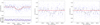 |
Fig. B.1 Transit modelling of the wiggle in TESS Sector 22 based on the photometry as extracted from PDCSAP (left), SAP (mid), and PATHOS (right). The MCMCI analysis does not lead to any transit detection when attempting to fit a transit in the SAP and PATHOS photometry. The outcomes depend on the extraction pipeline, which plays against the genuineness of the putative transit event as confirmed by the BIC as well (see text for further details). |
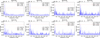 |
Fig. B.2 GLS periodograms of different activity indicators as inferred from the HARPS-N RV time series with the FAP levels at 1% and 0.1% marked as dashed and dotted red lines, respectively. First row: from left to right FWHM, FWHMSN, A, and ASN. Second row: from left to right BIS, γ, log R′HK, and Hα, where the latter two were subject to a pre-whitening. The most prominent peak is always at ∼20 days, which is likely the stellar rotation period (Prot,*). |
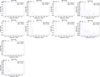 |
Fig. B.3 GLS periodograms of the five TESS sectors (SAP photometry) computed after removing all the transit windows. First row: from left to right sector 22, 48, 49, and 75. Second row: same as first row, but after subtracting the most prominent peak. Third row: sector 76. Fourth row: sector 76 after subtracting the most prominent peak. The most prominent peak is always at Prot,* ∼ 20 days, except for Sector 75 (last panels in the first and second row) where the second (Prot,*/3) and first (Prot,*/2) harmonic of Prot,* appear. |
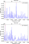 |
Fig. B.4 Top. GLS periodogram of the RV residuals obtained after subtracting the Keplerian signals of the four transiting planets to the HARPS-N detrended RV time series (Sect. 5.3). The most prominent peak is the second harmonic of Prot,*. The vertical dotted red line marks the signal of TOI-5624 f at ∼ 45 d. Bottom. Same but after further subtracting the signal at ∼ 6.4 d. The signal at ~45 d becomes the most prominent one with the second highest peak being Prot,*/2. |
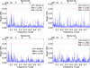 |
Fig. B.5 GLS periodograms of the FHWM (first row) and γ (second row) as computed from the HARPS-N time series after a pre-whitening. Although not always significant, we systematically observe peaks at ∼10d (first column) and ∼6.4d (second column), which we ascribe to the first (Prot,*/2) and second (Prot,*/3) harmonics of the stellar rotation period (Prot,*). A similar behaviour is seen in the other RV-related activity indicators (not shown here). |
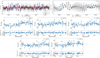 |
Fig. B.6 RV analysis performed with pyaneti. Top-left: Time series of the HARPS-N TERRA RV measurements (blue points). The inferred models for the five-planet and GP signals are shown with red and blue thick lines, respectively, whereas the combined signal is displayed in black. Topright: Time series of the FWHM of the DRS cross-correlation functions (blue points). The black thick line marks the inferred GP model, whereas the grey shaded areas show its 1σ and 2σ credible intervals. Second and third rows, from top to bottom and left to right: Phase-folded RV curves of TOI-5624 b, c, d, e, and f, and best-fitting Keplerian models (thick black lines). In each panel, the nominal uncertainties of the data points and the jitter contribution are shown with thin and thick blue lines, respectively. |
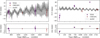 |
Fig. B.7 Same as Fig. 4, but assuming the four-planet configuration. Left: TOI-5624 d. Right: TOI-5624 e. |
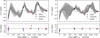 |
Fig. B.8 O–C diagrams of TOI-5624 e for two additional dynamical analyses to test the robustness of the five-planet solution. Left: Fit obtained from the TTV+RV analysis after adopting a broader prior on the orbital period of planet f (Pf ∈ [1,50] d), hence allowing configurations where the planet may lie between TOI-5624 d and e. Right: Fit obtained assuming again Pf ∈ [1,50] d, but using the transit mid-times only (i.e. excluding the RV dataset). Like the nominal analysis, both these analyses consistently conclude that only an external perturber may justify the TTVs of TOI-5624 e. |
 |
Fig. B.9 Stability analysis of the TOI-5624 planetary system focussing on planet f. We varied the orbital period, Pf and the eccentricity ef (left) and the longitude of the node, Ωf, and the inclination, If (right), while keeping all the remaining orbital parameters fixed at their best-fit values (Tab. 2). The step size is 0.015 day in the orbital period, 0.0025 in the eccentricity, and 1° in the longitude of the node and inclination. Plots are colour-coded according to the stability indicator calculated from the frequency analysis of the mean longitude of TOI-5624 f. Red points correspond to highly unstable orbits, while blue points correspond to orbits that are likely to be stable on Gyr timescales. The vertical dashed line (left) corresponds to the 2:1 MMR between planets e and f. The black dot along with its error bars highlights the RV-based best-fit solution Pf,RV = |


Appendix C Additional tables
Log of CHEOPS observations.
Polynomial detrending baseline applied to the TESS LCs within the MCMCI analysis.
Polynomial detrending baseline applied to the CHEOPS LCs within the MCMCI analysis.
HARPS-N derived parameters of TOI-5624, as inferred using the multi-dimensional GP approach implemented in pyaneti.
Posteriors of the TOI-5624 system from the two tested dynamical scenarios.
All Tables
Radial velocities, RV, as inferred from the SN fit onto the centred HARPS-N CCFs with their errors σRV. They are followed by the ancillary parameters used for the detrending (i.e. FWHMSN, Hα, γ, and NaD2) and by the detrended RV values (RVdet) with their errors which also account for the jitter (σRV(det+jitter)).
Radial velocities, RV, as extracted from the centred SOPHIE CCFs with their errors σRV. They are followed by the CCF-related parameters (i.e. FWHM, A, and BIS), the log R′HK, and by the detrended RV values (RVdet) with their errors which also account for the jitter (σRV(det+jitter)).
Polynomial detrending baseline applied to the TESS LCs within the MCMCI analysis.
Polynomial detrending baseline applied to the CHEOPS LCs within the MCMCI analysis.
HARPS-N derived parameters of TOI-5624, as inferred using the multi-dimensional GP approach implemented in pyaneti.
All Figures
|
Fig. 1 TTVs with respect to linear ephemerides for TOI-5624 b, c, d, and e (top to bottom). The grey shaded area marks the 1σ uncertainty region of the linear ephemerides’ model. |
| In the text | |
|
Fig. 2 Folded and detrendend LCs of planets b to e (top to bottom) as observed by CHEOPS (left) and TESS (right). Blue dots are the original data points, while black dots show the 20-minute binned data. The best-fit transit model is superimposed in red and the corresponding residuals are shown in the bottom panel of each plot. |
| In the text | |
|
Fig. 3 Detrended RV time series folded according to the period of TOI-5624b (top-left), TOI-5624c (top-right), TOI-5624d (middleleft), TOI-5624e (middle-right), and TOI-5624f (bottom-left) after removing the Keplerian signals of the other planets as inferred from the MCMCI analysis. The marker colour distinguishes the two different instruments (light blue for HARPS-N and orange for SOPHIE), while the red line represents the inferred model. The jitter contribution in the error bars is highlighted in grey. The RV semi-amplitudes are measured at the 6.9, 2.5, 2.2, 3.1, and 3.5σ level for planets b, c, d, e, and f, respectively. |
| In the text | |
|
Fig. 4 O–C diagrams of TOI-5624 d (top) & e (bottom) along with the residuals (res) with respect to the best-fit model when assuming the five-planet configuration. The best-fit TRADES model is shown as a black line, while the shaded areas display the 1σ, 2σ, and 3σ confidence intervals. |
| In the text | |
|
Fig. B.1 Transit modelling of the wiggle in TESS Sector 22 based on the photometry as extracted from PDCSAP (left), SAP (mid), and PATHOS (right). The MCMCI analysis does not lead to any transit detection when attempting to fit a transit in the SAP and PATHOS photometry. The outcomes depend on the extraction pipeline, which plays against the genuineness of the putative transit event as confirmed by the BIC as well (see text for further details). |
| In the text | |
|
Fig. B.2 GLS periodograms of different activity indicators as inferred from the HARPS-N RV time series with the FAP levels at 1% and 0.1% marked as dashed and dotted red lines, respectively. First row: from left to right FWHM, FWHMSN, A, and ASN. Second row: from left to right BIS, γ, log R′HK, and Hα, where the latter two were subject to a pre-whitening. The most prominent peak is always at ∼20 days, which is likely the stellar rotation period (Prot,*). |
| In the text | |
|
Fig. B.3 GLS periodograms of the five TESS sectors (SAP photometry) computed after removing all the transit windows. First row: from left to right sector 22, 48, 49, and 75. Second row: same as first row, but after subtracting the most prominent peak. Third row: sector 76. Fourth row: sector 76 after subtracting the most prominent peak. The most prominent peak is always at Prot,* ∼ 20 days, except for Sector 75 (last panels in the first and second row) where the second (Prot,*/3) and first (Prot,*/2) harmonic of Prot,* appear. |
| In the text | |
|
Fig. B.4 Top. GLS periodogram of the RV residuals obtained after subtracting the Keplerian signals of the four transiting planets to the HARPS-N detrended RV time series (Sect. 5.3). The most prominent peak is the second harmonic of Prot,*. The vertical dotted red line marks the signal of TOI-5624 f at ∼ 45 d. Bottom. Same but after further subtracting the signal at ∼ 6.4 d. The signal at ~45 d becomes the most prominent one with the second highest peak being Prot,*/2. |
| In the text | |
|
Fig. B.5 GLS periodograms of the FHWM (first row) and γ (second row) as computed from the HARPS-N time series after a pre-whitening. Although not always significant, we systematically observe peaks at ∼10d (first column) and ∼6.4d (second column), which we ascribe to the first (Prot,*/2) and second (Prot,*/3) harmonics of the stellar rotation period (Prot,*). A similar behaviour is seen in the other RV-related activity indicators (not shown here). |
| In the text | |
|
Fig. B.6 RV analysis performed with pyaneti. Top-left: Time series of the HARPS-N TERRA RV measurements (blue points). The inferred models for the five-planet and GP signals are shown with red and blue thick lines, respectively, whereas the combined signal is displayed in black. Topright: Time series of the FWHM of the DRS cross-correlation functions (blue points). The black thick line marks the inferred GP model, whereas the grey shaded areas show its 1σ and 2σ credible intervals. Second and third rows, from top to bottom and left to right: Phase-folded RV curves of TOI-5624 b, c, d, e, and f, and best-fitting Keplerian models (thick black lines). In each panel, the nominal uncertainties of the data points and the jitter contribution are shown with thin and thick blue lines, respectively. |
| In the text | |
|
Fig. B.7 Same as Fig. 4, but assuming the four-planet configuration. Left: TOI-5624 d. Right: TOI-5624 e. |
| In the text | |
|
Fig. B.8 O–C diagrams of TOI-5624 e for two additional dynamical analyses to test the robustness of the five-planet solution. Left: Fit obtained from the TTV+RV analysis after adopting a broader prior on the orbital period of planet f (Pf ∈ [1,50] d), hence allowing configurations where the planet may lie between TOI-5624 d and e. Right: Fit obtained assuming again Pf ∈ [1,50] d, but using the transit mid-times only (i.e. excluding the RV dataset). Like the nominal analysis, both these analyses consistently conclude that only an external perturber may justify the TTVs of TOI-5624 e. |
| In the text | |
|
Fig. B.9 Stability analysis of the TOI-5624 planetary system focussing on planet f. We varied the orbital period, Pf and the eccentricity ef (left) and the longitude of the node, Ωf, and the inclination, If (right), while keeping all the remaining orbital parameters fixed at their best-fit values (Tab. 2). The step size is 0.015 day in the orbital period, 0.0025 in the eccentricity, and 1° in the longitude of the node and inclination. Plots are colour-coded according to the stability indicator calculated from the frequency analysis of the mean longitude of TOI-5624 f. Red points correspond to highly unstable orbits, while blue points correspond to orbits that are likely to be stable on Gyr timescales. The vertical dashed line (left) corresponds to the 2:1 MMR between planets e and f. The black dot along with its error bars highlights the RV-based best-fit solution Pf,RV = |
| In the text | |
Current usage metrics show cumulative count of Article Views (full-text article views including HTML views, PDF and ePub downloads, according to the available data) and Abstracts Views on Vision4Press platform.
Data correspond to usage on the plateform after 2015. The current usage metrics is available 48-96 hours after online publication and is updated daily on week days.
Initial download of the metrics may take a while.