| Issue |
A&A
Volume 693, January 2025
|
|
|---|---|---|
| Article Number | A90 | |
| Number of page(s) | 18 | |
| Section | Planets, planetary systems, and small bodies | |
| DOI | https://doi.org/10.1051/0004-6361/202451300 | |
| Published online | 07 January 2025 | |
Radii, masses, and transit-timing variations of the three-planet system orbiting the naked-eye star TOI-396★
1
Austrian Academy of Sciences,
Schmiedlstrasse 6,
8042
Graz,
Austria
2
Dipartimento di Fisica, Università degli Studi di Torino,
via Pietro Giuria 1,
10125
Torino,
Italy
3
Department of Physics and Astronomy, Uppsala University,
Box 516,
Uppsala
75120,
Sweden
4
INAF, Osservatorio Astronomico di Padova,
Vicolo dell’Osservatorio 5,
35122
Padova,
Italy
5
Weltraumforschung und Planetologie, Physikalisches Institut, University of Bern,
Gesellschaftsstrasse 6,
3012
Bern,
Switzerland
6
INAF, Osservatorio Astrofisico di Torino,
Via Osservatorio, 20,
10025
Pino Torinese To,
Italy
7
Department of Physics, University of Warwick,
Coventry
CV4 7AL,
UK
8
Centre for Exoplanets and Habitability, University of Warwick,
Gibbet Hill Road,
Coventry
CV4 7AL,
UK
9
Departamento de Física Teórica e Experimental, Universidade Federal do Rio Grande do Norte, Campus Universitário,
Natal,
RN 59072-970,
Brazil
10
Leiden Observatory, University of Leiden,
PO Box 9513,
2300 RA
Leiden,
The Netherlands
11
Chalmers University of Technology, Department of Space, Earth and Environment, Onsala Space Observatory,
SE-439 92
Onsala,
Sweden
12
INAF – Osservatorio Astrofisico di Arcetri,
Largo E. Fermi 5
Florence,
Italy
13
Instituto de Astrofísica e Ciências do Espaço, Universidade do Porto, CAUP, Rua das Estrelas,
4150-762
Porto,
Portugal
14
School of Physics and Astronomy,
Physical Science Building, North Haugh,
St Andrews,
UK
15
Rhenish Institute for Environmental Research, Dep. of Planetary Research, University of Cologne,
Aachener Str. 209,
50931
Cologne,
Germany
16
Institute of Planetary Research, German Aerospace Center (DLR),
Rutherfordstrasse 2,
12489
Berlin,
Germany
17
Thüringer Landessternwarte Tautenburg,
Sternwarte 5,
07778
Tautenburg,
Germany
18
University Observatory Munich, Ludwig-Maximilians-Universität,
Scheinerstr. 1,
81679
Munich,
Germany
19
European Southern Observatory,
Alonso de Cordova 3107, Vitacura, Casilla,
19001
Santiago,
Chile
20
European Southern Observatory,
Alonso de Cordova 3107, Vitacura,
Santiago de Chile,
Chile
21
Centro de Astrobiología (CAB), CSIC-INTA,
Camino Bajo del Castillo s/n,
28692
Villanueva de la Cañada (Madrid),
Spain
22
McDonald Observatory, The University of Texas,
Austin,
TX,
USA
23
Center for Planetary Systems Habitability, The University of Texas,
Austin,
TX,
USA
24
Department of Astronomy & Astrophysics, University of Chicago,
Chicago,
IL
60637,
USA
25
Astronomy Department and Van Vleck Observatory, Wesleyan University,
Middletown,
CT
06459,
USA
26
Departamento de Física e Astronomia, Faculdade de Ciências, Universidade do Porto, Rua do Campo Alegre,
4169-007
Porto,
Portugal
27
Department of Astronomy of the University of Geneva,
chemin Pegasi 51,
1290
Versoix,
Switzerland
28
Astrobiology Center, NINS,
2-21-1 Osawa, Mitaka,
Tokyo
181-8588,
Japan
29
National Astronomical Observatory of Japan, NINS,
2-21-1 Osawa, Mitaka,
Tokyo
181-8588,
Japan
30
Astronomical Science Program, Graduate University for Advanced Studies, SOKENDAI,
2-21-1, Osawa, Mitaka,
Tokyo,
181-8588,
Japan
31
Instituto de Astrofísica de Canarias (IAC),
calle Vía Láctea s/n,
38205
La Laguna,
Tenerife,
Spain
32
Departamento de Astrofísica, Universidad de La Laguna (ULL),
38206
La Laguna,
Tenerife,
Spain
33
Institute of Astronomy, Faculty of Physics, Astronomy and Informatics, Nicolaus Copernicus University,
Grudziądzka 5,
87-100
Toruń,
Poland
34
Department of Physics and Astronomy, McMaster University,
1280 Main St W,
Hamilton,
ON
L8S 4L8,
Canada
35
Department of Physics, ETH Zurich,
Wolfgang-Pauli-Strasse 2,
8093
Zurich,
Switzerland
★★ Corresponding author; This email address is being protected from spambots. You need JavaScript enabled to view it.
Received:
28
June
2024
Accepted:
20
November
2024
Abstract
Context. TOI-396 is an F6 V bright naked-eye star (V ≈ 6.4) orbited by three small (Rp ≈ 2 R⊕) transiting planets discovered thanks to space-based photometry from two TESS sectors. The orbital periods of the two innermost planets, namely TOI-396 b and c, are close to the 5:3 commensurability (Pb ~ 3.6 d and Pc ~ 6.0 d), suggesting that the planets might be trapped in a mean motion resonance (MMR).
Aims. To measure the masses of the three planets, refine their radii, and investigate whether planets b and c are in MMR, we carried out HARPS radial velocity (RV) observations of TOI-396 and retrieved archival high-precision transit photometry from four TESS sectors.
Methods. We extracted the RVs via a skew-normal fit onto the HARPS cross-correlation functions and performed a Markov chain Monte Carlo joint analysis of the Doppler measurements and transit photometry, while employing the breakpoint method to remove stellar activity from the RV time series. We also performed a transit timing variation (TTV) dynamical analysis of the system and simulated the temporal evolution of the TTV amplitudes of the three planets following an N-body numerical integration.
Results. Our analysis confirms that the three planets have similar sizes (Rb = 2.004−0.047+0.045 R⊕ ; Rc = 1.979−0.051+0.054 R⊕; Rd = 2.001−0.064+0.063 R⊕) and is thus in agreement with previous findings. However, our measurements are ~ 1.4 times more precise thanks to the use of two additional TESS sectors. For the first time, we have determined the RV masses for TOI-396 b and d, finding them to be Mb = 3.55−0.96+0.94 M⊕ and Md = 7.1 ± 1.6 M⊕, which implies bulk densities of ρb = 2.44−0.68+0.69 g cm−3 and ρd = 4.9−1.1+1.2 g cm−3, respectively. Our results suggest a quite unusual system architecture, with the outermost planet being the densest. Based on a frequency analysis of the HARPS activity indicators and TESS light curves, we find the rotation period of the star to be Prot,⋆ = 6.7 ± 1.3 d, in agreement with the value predicted from log R′HK-based empirical relations. The Doppler reflex motion induced by TOI-396 c remains undetected in our RV time series, likely due to the proximity of the planet’s orbital period to the star’s rotation period. We also discovered that TOI-396 b and c display significant TTVs. While the TTV dynamical analysis returns a formally precise mass for TOI-396 c of Mc,dyn = 2.24−0.67+0.13 M⊕, the result might not be accurate, owing to the poor sampling of the TTV phase. We also conclude that TOI-396 b and c are close to but out of the 5:3 MMR.
Conclusions. A TTV dynamical analysis of additional transit photometry evenly covering the TTV phase and super-period is likely the most effective approach for precisely and accurately determining the mass of TOI-396 c. Our numerical simulation suggests TTV semi-amplitudes of up to five hours over a temporal baseline of ~ 5.2 years, which should be duly taken into account when scheduling future observations of TOI-396.
Key words: techniques: photometric / techniques: radial velocities / planets and satellites: fundamental parameters / stars: fundamental parameters
Based on observations performed with the 3.6 m telescope at the European Southern Observatory (La Silla, Chile) under programmes 1102.C-0923, 1102.C-0249, 0102.C-0584, and 60.A-9700.
© The Authors 2025
 Open Access article, published by EDP Sciences, under the terms of the Creative Commons Attribution License (https://creativecommons.org/licenses/by/4.0), which permits unrestricted use, distribution, and reproduction in any medium, provided the original work is properly cited.
This article is published in open access under the Subscribe to Open model. This email address is being protected from spambots. You need JavaScript enabled to view it. to support open access publication.
1 Introduction
Multi-planet systems enable us to place significantly stronger constraints on formation and evolution mechanisms compared to single-planet systems (e.g. Lissauer et al. 2011; Fabrycky et al. 2014; Winn & Fabrycky 2015; Mishra et al. 2023). As a matter of fact, the temporal evolution of the gas content in the proto-planetary disc influences planet migration (e.g. Lin & Papaloizou 1979; Goldreich & Tremaine 1980; Tanaka et al. 2002; D’Angelo & Lubow 2008; Alexander & Armitage 2009), which shapes the orbital architecture of a planetary system. The latter is further expected to correlate with the planet composition (e.g. Thiabaud et al. 2014, 2015; Walsh et al. 2015; Bergner et al. 2020; Li et al. 2020) that can be inferred once the physical parameters of the planets are known (e.g. Dorn et al. 2017; Otegi et al. 2020b; Leleu et al. 2021; Haldemann et al. 2024).
If planets are found in mean motion resonance (MMR; e.g. Lee & Peale 2002; Correia et al. 2018), systems can also shed light on the migration mechanisms during formation as well as on the impact of tidal effects occurring later on (e.g. Delisle et al. 2012; Izidoro et al. 2017). In addition, planets in or close to MMR likely exhibit transit timing variations (TTVs; see e.g. Agol et al. 2005; Agol & Fabrycky 2018; Leleu et al. 2021) that enable one to infer planetary masses without necessarily relying on radial velocity (RV) measurements, which are not always possible (e.g. Hatzes 2016).
Multi-planet systems also give insights into correlations between physical and orbital parameters of exoplanets. For example, Weiss et al. (2018) noticed that planets in adjacent orbits usually show similar radii, hence the ‘peas in a pod’ label to describe this scenario. Weiss et al. (2018) further noticed that the outermost planet is the largest in the majority of cases, which agrees with the observed bulk planet density (ρp) trend highlighted by Mishra et al. (2023), where ρp decreases with the distance from the stellar host, as outer planets are expected to be richer in volatiles (thus bigger and less dense).
The object TOI-396 represents an interesting laboratory to test these theories, as it is the brightest star known so far to host three transiting planets (Vanderburg et al. 2019) after ν2 Lupi (Delrez et al. 2021). After analysing two sectors from the Transiting Exoplanet Survey Satellite (TESS; Ricker et al. 2015), Vanderburg et al. (2019) found that the three planets have radii of ∼ 2 R⊕ and orbital periods of ∼3.6, ∼ 6.0, and ∼11.2 d, with TOI-396 c and b showing a period commensurability close to the 5:3 ratio. Following the notation introduced in Mishra et al. (2023), the three planets are ‘similar’ in terms of radii, and one may wonder whether this architecture class is kept also in the mass-period diagram. Mishra et al. (2023) found a positive and strong correlation of the coefficients of similarity between radii and masses, though exceptions are possible (e.g. Weiss & Marcy 2014; Otegi et al. 2020a, 2022).
In this work, we complement the photometric analysis of new TESS light curves (LCs) with RV observations taken with the High Accuracy Radial Velocity Planet Searcher (HARPS; Mayor et al. 2003) spectrograph to refine the planet radii and constrain for the first time the planetary masses. Considering the possible 5:3 MMR between TOI-396 c and b, we also simulate the evolution in time of the TTV amplitudes. This paper is organised as follows: Section 2 presents the stellar properties, and Sect. 3 describes the photometric and RV data. After outlining the method to jointly analyse the TESS LCs and the HARPS RV time series in Sect. 4, we present the corresponding results in Sect. 5. We attempt to dynamically model TTV and RV data simultaneously and track the temporal evolution of the TTV signals in Sect. 6, and we study the planets’ internal structure in Sect. 7 and explore the prospects for characterising the system with the James Webb Space Telescope (JWST; Gardner et al. 2006) in Sect. 8. Finally Sect. 9 gathers the conclusions.
2 Host star characterisation
TOI-396 is an F6 V (Gray et al. 2006) bright naked-eye star with an apparent visual magnitude of V ≈ 6.4 (Perryman et al. 1997). It is located ∼31.7 pc away and is visible in the constellation of Fornax in the southern hemisphere. It is member of a visual binary system and its companion HR 858 B is a faint M-dwarf (G ∼ 16 mag), about 8.4″ away from the main component.
We co-added 78 HARPS spectra (see Sect. 3.2 for further details) and then modelled it with Spectroscopy Made Easy1 (SME; Piskunov & Valenti 2017) version 5.2.2. SME computes synthetic spectra from a grid of well established stellar atmosphere models and adjusts a chosen free parameter based on comparison with the observed spectrum. Here we used the stellar atmosphere grid ATLAS 12 (Kurucz 2013) together with atomic line lists from the VALD database (Piskunov et al. 1995) in order to produce the synthetic spectra. We modelled one parameter at a time utilising spectral features sensitive to different photospheric parameters iterating until convergence of all free parameters. Throughout the modelling, we held the macro- and micro-turbulent velocities, vmac and vmic , fixed to 6 km s−1 (Doyle et al. 2014) and 1.34 km s−1 (Bruntt et al. 2010), respectively. A description of the modelling procedure is detailed in Persson et al. (2018). Finally, we obtained Teff = 6354 ± 70 K, [Fe/H] = 0.025 ± 0.050, log g = 4.30 ± 0.06, and v sin i⋆ = 7.5 ± 0.2 km s−1.
To double-check the derived spectroscopy parameters we performed an additional analysis employing ARES+MOOG (Sousa et al. 2021; Sousa 2014; Santos et al. 2013). In detail, we used the latest version of ARES2 (Sousa et al. 2007, 2015) to consistently measure the equivalent widths (EW) for the list of iron lines presented in Sousa et al. (2008). Following a minimisation process, we then find the ionisation and excitation equilibria to converge for the best set of spectroscopic parameters. This process uses a grid of Kurucz model atmospheres (Kurucz 1993) and the radiative transfer code MOOG (Sneden 1973). We obtained Teff = 6389 ± 67 K, [Fe/H] = −0.014 ± 0.045 dex, log g = 4.58 ± 0.11, and vmic = 1.54 ± 0.04 km s−1. In this process we also derived a more accurate trigonometric surface gravity (log ցtrIg = 4.34 ± 0.02) using recent Gaia data following the same procedure as described in Sousa et al. (2021). In the end ARES+MOOG provides consistent values when compared with the ones derived with SME.
Using the SME stellar atmospheric parameters, we determined the abundances of Mg and Si following the classical curve-of-growth analysis method described in Adibekyan et al. (2012, 2015). Similar to the stellar parameter determination, we used ARES to measure the EWs of the spectral lines of these elements and a grid of Kurucz model atmospheres (Kurucz 1993) along with the radiative transfer code MOOG to convert the EWs into abundances, assuming local thermodynamic equilibrium.
The stellar radius R⋆ , mass M⋆ , and age t⋆ were derived homogeneously using the isochrone placement algorithm (Bonfanti et al. 2015, 2016) and its capability of interpolating a flexible set of input parameters within pre-computed grids of PARSEC3 v1.2S (Marigo et al. 2017) isochrones and tracks. For each magnitude listed in Table 1, we performed an isochrone placement run by inserting the spectroscopic parameters derived above, the Gaia parallax π (Gaia Collaboration 2023, offset- corrected following Lindegren et al. 2021), and the magnitude value to obtain an estimate for the stellar radius, mass, and age along with their uncertainties. From these results, we built the corresponding Gaussian probability density functions (PDFs) and then we merged (i.e. we summed) the PDFs derived from the different runs to obtain robust estimates for R⋆, M⋆ , and t⋆ . The radius R⋆ derives essentially from Teff, π, and the stellar magnitude, while M⋆ and t⋆ are much more model-dependent; therefore we conservatively inflated their internal uncertainties by 4% and 20%, respectively, following Bonfanti et al. (2021). Our adopted stellar parameters are listed in Table 1.
Stellar properties of TOI-396.
3 Observational data
3.1 TESS photometry
As presented in Vanderburg et al. (2019), TOI-396 was photometrically monitored by TESS during the first year of its nominal mission in Sector 3 from 20 September to 17 October 2018 (UT) in CCD 2 of Camera 2, and in Sector 4 from 19 October to 14 November 2018 (UT) in CCD 2 of Camera 1. TOI-396 was later re-observed by TESS during the first year of its extended mission in Sector 30 from 23 September to 20 October 2020 (UT) in CCD 2 of Camera 2, and in Sector 31 from 22 October to 16 November 2020 (UT) in CCD 2 of Camera 1. All data were collected at a 2-minute cadence, except for Sector 3 for which TESS only sent down data at 30-minute cadence.
We analyse all available TESS time series, including the Sector 3 and 4 data already presented in Vanderburg et al. (2019). For Sector 3 we used the TESS Asteroseismic Science Operation Center (TASOC) photometry (Handberg et al. 2021; Lund et al. 2021), while for the other sectors we analysed the Presearch Data Conditioning Simple Aperture Photometry (PDC- SAP) LCs generated by the TESS Science Processing Operation Center (SPOC) pipeline Jenkins et al. (2016), which removes the majority of instrumental artefacts and systematic trends (Smith et al. 2012; Stumpe et al. 2012, 2014). We rejected those data marked with a bad quality flag and we performed a 5 medianabsolute-deviation (MAD) clipping of flux data points. After that, we built our custom LCs by splitting the TESS sectors in temporal windows centred around the transit events keeping ~ 4 h of out-of-transit data points both before and after the transit for de-trending purposes. We ended up with 41 TESS LCs reporting the epoch of observation (t), the flux and its error, and further ancillary vectors available from the TESS science data product, that is MOM_CENTR1, MOM_CENTR2 (hereafter denoted with x and y, respectively), POS_CORR1, and POS_CORR2 (hereafter denoted with pc1 and pc2, respectively)4.
3.2 HARPS high-resolution spectroscopy
We performed the radial velocity (RV) follow-up of TOI-396 with the HARPS spectrograph mounted at the ESO-3.6 m telescope at La Silla Observatory (Chile). We acquired 77 high resolution (R≈ 115 000) spectra between 31 January and 27 July 2019 (UT), covering a baseline of ~ 177 days, as part of the follow-up programs of TESS systems carried out with the HARPS spectrograph (IDs: 1102.C-0923, 1102.C-0249, 0102.C- 0584; PIs: Gandolfi, Armstrong, De Medeiros). One additional spectrum was acquired during a technical night (ID: 60.A-9700) in February 2019. Following Dumusque et al. (2011b), we averaged out p-mode stellar pulsations by setting the exposure time to 900 s, which led to a median signal-to-noise (S/N) ratio of ~320 per pixel at 550 nm. We used the second fibre of the HARPS spectrograph to simultaneously observe a Fabry-Perot lamp and trace possible instrumental drift down to the sub-metre per second level (Wildi et al. 2010). We reduced the data using the dedicated HARPS data reduction software (DRS; Pepe et al. 2002; Lovis & Pepe 2007) and computed the cross-correlation function (CCF) for each spectrum using a G2 numerical mask (Baranne et al. 1996).
We then performed a skew-normal (SN) fit on each CCF (Simola et al. 2019) in order to extract the stellar radial velocity along with its error, the full width at half maximum (FWHMSN), the contrast (A), and the skewness parameter (γ) of the CCF. The advantages of using an SN-fit rather than a Normal fit are thoroughly discussed in Simola et al. (2019), while the SN- fitting details are outlined in, for example, Bonfanti et al. (2023); Luque et al. (2023); Fridlund et al. (2024). After the SN-based extraction, we ended up with an RV time series, whose ancillary vectors (FWHMSN, A, γ) are the activity indicators used to constrain the polynomial basis to model and de-trend the RV component of the stellar activity (see Table A.1).
As stellar activity is not stationary, the correlations between the RV observations and the activity indicators are expected to change over time as discussed in Simola et al. (2022), who proposed to apply the breakpoint (bp) technique (Bai & Perron 2003) to check whether these correlation changes are statistically significant. If so, the bp algorithm finds the optimal locations of correlation changes, which defines the segmentation characterised by the lowest Bayesian Information Criterion (BIC; Schwarz 1978). Indeed, we found one breakpoint at observation 48 (BJD = 2458667.940719; ΔBIC ≈ −14 with respect to the zero-breakpoint solution). Thus, we split our RV time series in two piecewise stationary segments and de-trended it on a chunkwise base, rather than performing a global de-trending over the whole time series, similarly to what has already been done in Bonfanti et al. (2023); Luque et al. (2023).
4 Methods
We jointly analysed the TESS LCs and the RV time series within a Markov chain Monte Carlo (MCMC) framework using the MCMCI code (Bonfanti & Gillon 2020). When fitting the TESS LCs extracted from Sector 3 that has a cadence of 30 min, we generated the transit model using a cadence of 2 min (the same as the other TESS sectors) and then rebinned it to 30 min following Kipping (2010), who warns that long-cadence photometry may lead to retrieve erroneous system parameters. We imposed Normal priors on the input stellar parameters (i.e. Teff, [Fe/H], R⋆ , and M⋆), as derived in Section 2 with a twofold aim: (i) the induced prior on the mean stellar density ρ⋆ (via M⋆ and R⋆ ) helps the convergence of the transit model; (ii) limb darkening (LD) coefficients for the TESS filter may be retrieved following interpolation within ATLAS 9-based5 grids that were pre-computed using the get_lds.py code6 by Espinoza & Jordán (2015). We then set Normal priors on the quadratic LD coefficients using the values coming from the grid interpolation (i.e. u1,TESS = 0.2318 ± 0.0065 and u2,TESS = 0.3085 ± 0.0028) after re-parameterising them following Holman et al. (2006). On the planetary side, we adopted unbounded (except for the physical limits) uniform priors on the transit depth dF, the impact parameter b, the orbital period P, the transit timing T0 , and the RV semi-amplitude K, while we set the eccentricity e = 0 and the argument of periastron ω = 90° for all planets. We come back to the assumption on the eccentricity below. The specific parameterisations of the jump parameters (aka step parameters) are outlined in Bonfanti & Gillon (2020).
The LCs and the RV time series were de-trended simultaneously during the MCMC analysis using polynomials. To assess the polynomial orders to be associated with the different detrending parameters for each time series, we first launch several MCMC preliminary runs made of 10 000 steps where we varied only one polynomial order at a time. We then selected the best de-trending baseline (see Table A.2) as the one having the lowest BIC. After that, we performed a preliminary MCMCI run comprising 200 000 steps to evaluate the contribution of both the white and red noise in the LCs following Pont et al. (2006); Bonfanti & Gillon (2020), so to properly rescale the photometric errors and get reliable uncertainties on the output parameters. Finally, three independent MCMCI runs comprising 200 000 steps each (burn-in length equal to 20%) were performed to build the posterior distributions of the output parameters after checking their convergence via the Gelman-Rubin statistic ( ; Gelman & Rubin 1992).
We also tested the possibility of eccentric orbits by imposing uniform priors on (  ) either bounded to imply e ≲ 0.3 or completely unbounded (except for the physical limits). The wider the eccentricity range to be explored by the MCMC scheme, the poorer the parameter convergence, which suggests that the available data are not enough to constrain the planetary eccentricities well. Moreover, the MCMCI runs with e ≠ 0 are disfavoured by the ΔBIC criterion (e.g. Kass & Raftery 1995; Trotta 2007) as well, in fact we obtained ΔBIC = BICe≠0 − BICe=0 ≳ +100. This is also in agreement with the simulations performed by Vanderburg et al. (2019), who suggested that the periods’ commensurability state of planets b and c is more likely maintained if the system is characterised by low eccentricities. Therefore, we adopted the circular solution as the reference one.
5 LC and RV data analysis results
5.1 Joint LC and RV analysis with linear ephemerides
As mentioned in Section 4, we set P and T0 as free parameters under the control of a uniform prior, which implies assuming linear ephemerides. With this setup, we improved the transit depth precision of all three planets by a factor ~1.4 if compared with the results of Vanderburg et al. (2019). This improvement level is consistent with having twice the number of data points with respect to the LC analysis performed by Vanderburg et al. (2019), as well as with low TTV amplitudes (see Section 5.2).
By combining the SN-fit onto the HARPS CCFs along with the bp method, we were able to estimate the masses of TOI-396 b and TOI-396d to  . (detections at the 3.8 and 4.5σ-level, respectively). Instead, we did not detect any significant Keplerian signal at the orbital period of TOI-396 c within the RV time series. In detail, we obtained a median
  (3σ upper limit
  ), which implies
  .
.
When combining the mass and radius values of the three planets, we obtain the following median estimates for the bulk planetary densities:  . We note that the RV-undetected TOI- 396 c would be the least dense planet, while the densest planet is the outermost one (i.e. TOI-396 d), which constitutes a quite atypical architecture within the observed exoplanet population (e.g. Ciardi et al. 2013; Weiss et al. 2018; Mishra et al. 2023). However, this conclusion is just tentative, given the uncertainties on the mean planetary densities. Moreover, the detection level of the RV-inferred parameters of TOI-396 c is not statistically significant. We further tested whether including the MINERVA-Australis (Addison et al. 2019) RV data (30 measurements as taken from Vanderburg et al. 2019) can help detect the elusive planet. However, it turned out that their precision level (~ 6 m s−1) is not high enough to improve the characterisation of the system. In other words, the RV semi-amplitudes we obtained are consistent and indistinguishable within the statistical fluctuation with what was derived from the more precise HARPS data set. This led us to further check that TOI-396 c indeed belongs to this system (Section 5.2) and to investigate the reason for its RV non-detection (Section 5.3).
5.2 Joint LC and RV analysis accounting for TTVs
As planet c is undetected in the RV time series, one may wonder whether TOI-396 c is a false positive. However, by using the VESPA tool (Morton 2012, 2015) that accounts for the constraints from the TESS LCs, imaging, and spectroscopy, Vanderburg et al. (2019) already computed that the false-positive probabilities (FPPs) are lower than 10−3 for all three planets.
In line with Vanderburg et al. (2019), we also confirmed that the Pc/Pb period ratio is commensurable and differs from the 5:3 ratio by less than 0.027%. As planets with orbits in, or close to, resonances are likely to show TTVs, we decided to repeat the same MCMC analysis outlined above, but enabling the transit timings of each transit event to vary to then compute the TTV amplitude with respect to the linear ephemerides model derived in Section 5.1. All jump parameters converged ( ). The medians of the posterior distributions of the most relevant system parameters along with the 68.3% confidence intervals are listed in Table 2. The phase-folded LCs of the three planets are shown in Figure 1, while the phase-folded RV time series are displayed in Figure 2. In particular, the middle panel of Fig. 2 shows that, after subtracting the RV signals of both planets b and d, the RV time series looks flat consistently with the non-detection of TOI-396 c.
This analysis gives  and confirms the RV detection of TOI- 396 b and TOI-396 d (at the 3.8 and 4.5σ-level, respectively) with
  and Md = 7.1 ± 1.6 M⊕. These outcomes are consistent with the results obtained from the analysis that assumes linear ephemerides (Section 5.1).
Fig. 3 shows the three planets of the system (star symbol) along with other exoplanets whose density is more significant than the 3σ level7 (circular marker) in the mass-radius (MR) diagram. The superimposed theoretical MR models as taken from Aguichine et al. (2021, A21) and Haldemann et al. (2024) help guide the eye; however, we warn the reader of possible degeneracies occurring in the MR plane. A thorough internal structure analysis of the well characterised TOI-396 b and d is presented in Section 7.
We found significant TTV signals for planet b and c (see Figure 4, Top and Middle panels) as expected from the commensurability of their periods. The TTV statistical significance of TOI-396 b and c is evident even by eye when comparing the data points location with the shaded regions that represent the 1σ uncertainties of the linear ephemerides. For each planet, we further quantified the reduced- characterising the TTV amplitudes via
 (1)
(1)
where Ntr, j is the number of transit event of the j-th planet. We obtained  for planets b, c, and d, respectively, which confirms the significance of the TTV amplitudes for TOI-396 b and c.
Furthermore, the TTV amplitudes of TOI-396 b and c exhibit a clear anti-correlation pattern that we highlight by superimposing the TTV measurements in Figure A.1. This is a typical signature of gravitational interaction between the two planets, which confirms that TOI-396 c belongs to the system despite its elusiveness in the RV time series. For each planet, the timing of each transit event and the corresponding TTV amplitude computed with respect to the linear ephemerides are listed in Table A.3.
System parameters as derived from the joint LC and RV analysis accounting for TTVs.
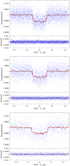 |
Fig. 1 TESS detrended and phase-folded LCs (blue dots) of TOI-396 b (top panel), TOI-396 c (middle panel), and TOI-396 d (bottom panel) with the transit model superimposed in red. The black markers are the binned data points (binning 20 min). |
5.3 Discussion regarding why TOI-396 c is not detected in the RV time series
Magnetic activity combined with stellar rotation induces RV variations that can hide, affect, or even mimic planetary signals (e.g. Queloz et al. 2001; Hatzes et al. 2010; Dumusque et al. 2011a; Haywood et al. 2014; Suárez Mascareño et al. 2017; Gandolfi et al. 2017). A possible explanation for the non-detection of the Doppler reflex motion induced by TOI-396 c is that stellar activity destructively interferes with the Keplerian signal of the planet. This may happen if the star has a rotation period comparable to the orbital period of the planet (e.g. Vanderburg et al. 2016). Disentangling the planetary signal from stellar activity and retrieving the Doppler motion induced by the orbiting planet would then be challenging (e.g. Dragomir et al. 2012; Kossakowski et al. 2022).
In order to investigate this hypothesis, we performed a frequency analysis of the line profile variation diagnostics (FWHM, contrast, and skewness) and activity indicators (log  and Hɑ indexes). Figure 5 displays the time series (left column), along with the respective generalised Lomb-Scargle (GLS, Zechmeister & Kürster 2009) periodograms (right column). We assessed the significance of the peaks detected in the power spectra by estimating their false alarm probability (FAP), that is the probability that noise could produce a peak with power higher than the one we found in the time series. To account for the possible presence of non-Gaussian noise in the data, we estimated the FAP using the bootstrap randomisation method (see, e.g., Murdoch et al. 1993; Kuerster et al. 1997; Hatzes 2019). Briefly, we computed the GLS periodogram of 105 mock time series obtained by randomly shuffling the data points along with their error bars, while keeping the timestamps fixed. We defined the FAP as the fraction of those mock periodograms whose highest power exceeds the power of the real data at any frequency. In the present work, we considered a peak to be significant if its false alarm probability is FAP < 0.1 %.
We found that the time series of the log  and Hɑ indexes display long-term trends likely due to the magnetic cycles of the star (Fig. 5, left column, first and third panels). In the Fourier domain, these trends translate into a significant (FAP < 0.1%) excess of power at frequencies lower than the spectral resolu- tion8 of our HARPS observations (Fig. 5, right column, first and third panels). We modelled these long-term signals as quadratic trends and subtracted the best-fitting parabolas from the respective time-series. The GLS periodograms of the residuals of the activity indicators display significant peaks between ~6 and 8 d (i.e, between ~0.0125 and 0.167 d−1 ; Fig. 5, yellow area). The peaks are equally spaced by ~0.0068 d−1, which coincides with a peak found in the periodogram of the window function. Given the current data at our disposal, we are not able to distinguish between true frequencies and aliases. Although not significant, the power spectra of the contrast and skewness show peaks in the same frequency range, suggesting that the rotation period of the star might be ~6–8 d.
We note that the periodogram of the FWHM also displays an excess of power at low frequencies. However, the corresponding peak remains below our 0.1 %-FAP significance threshold (see Fig. 5, second to last panel). Yet, if we apply the same procedure described above and remove this signal by fitting a quadratic trend to the FWHM time series, we find no significant peak in the residuals.
The projected equatorial velocity of the star (v sin i⋆ = 7.5 ± 0.2 km s−1), along with its radius (R⋆ = 1.258 ± 0.019 R⊙), yields an upper limit for the rotation period of  . Using the mean value9 of
  , we inferred a stellar rotation period of 6.7 ± 1.3 d and 6.9 ± 1.3 d from the empirical equations of Noyes et al. (1984) and Mamajek & Hillenbrand (2008), respectively. In addition, by inputting the isochronal age into the gyrochronological relation from Barnes (2010), we computed a stellar rotation period of
  . These results corroborate our interpretations that the peaks between 6 and 8 d significantly detected in the power spectra of the activity indicators originate from stellar rotation.
To check whether a quasi-periodic signal compatible with ~7 d is also present in the photometric data, for each TESS sector we extracted custom LCs from pixel data using lightkurve (Lightkurve Collaboration 2018). In detail, we adopted the default quality bitmask and set the aperture to ‘all’, which corresponds to an aperture larger than the one used by the official SAP pipeline. In fact, larger apertures mitigate the effect of slow image drifts that could interfere with slow flux changes, such as the 6–8 d rotation period signals we aim to detect. After removing the temporal windows containing the transit events, we computed the GLS periodograms of these lightkurve-based LCs. The FAP was computed following the same bootstrap technique outlined above for the RV activity indicators. The four periodograms (Fig. A.2, first column) exhibit very significant peaks at ∼ 7.7, 7.9, 7.5, and 6.8 days for TESS Sectors 3, 4, 30, and 31, respectively. Except for Sector 30, they are not the most prominent peaks; however, they persist even after removing the most significant signals (Fig. A.2, second column). Whereas we acknowledge that the likely rotation period of the star is close to the first harmonic of the orbital period of TESS around the Earth  , the photometric signal at 6–8 d is significant in all the four TESS sectors and persists after prewhitening the data. This signal is consistent with the rotation period detected in the HARPS activity indicators and inferred from log
  , v sin i⋆ , and gyrochronology, suggesting it is astrophysical in nature and due to the presence of active regions carried around by stellar rotation. Assuming the log
  -based Prot,⋆ = 6.7 ± 1.3 d as our reference estimate, the orbital period of TOI-396 c (Pc ~ 6 d) is close to Prot,⋆ , which may explain the non-detection of planet c within the RV time series.
If some kind of destructive interference between the Keplerian signal of planet c and the stellar activity has occurred, any artificial Keplerian signals with period P = Pc added to the observed RV time series should in principle be retrieved. To test this hypothesis, we considered Keplerian signals of the following form
![Mathematical equation: $R{V_{{\rm{art}}}} = - {K_{{\rm{art}}}}\sin \left[ {{{2\pi } \over P}\left( {t - {T_0}} \right)} \right]$](/articles/aa/full_html/2025/01/aa51300-24/aa51300-24-eq68.png) (2)
(2)
and generated four different RV time series by separately adding to the HARPS time series synthetic RV signals following Equation (2) with P = Pc, T0 = T0,c, and Kart = Kin, where Kin are the four different amplitude values listed in the first column of Table 3. For each RV time series, we then performed an MCMCI analysis to retrieve the RV semi-amplitude of the artificial signal (Kout ; see Table 3).
We note that the resulting Kout ≈ Kin + Kc, where Kc =  is the RV semi-amplitude of planet c as derived from the analysis on the original RV time series. As we essentially retrieved what we inserted in the HARPS time series, we may conclude that the destructive interference between the RV signals induced by the star and by planet c has already occurred and any further RV signal added to the RV time series is detected.
As Prot,⋆ is not exactly equal to Pc , we then repeated the test outlined above, but this time we injected into the original HARPS time series artificial Keplerian signals with P = Prot,⋆. The Kout values obtained by the MCMC analyses depending on the different Kin values are reported in Table 4. The Kout values are systematically and significantly smaller than the corresponding Kin values, which a posteriori supports the conclusion that the stellar rotation period is around 6–8 d. Furthermore, a planet with this orbital period would be firmly detected if its RV semi-amplitude were greater than Kd, which is the largest RV semi-amplitude detected for this system. Instead, by injecting a Keplerian signal with Kin = Kd and P = Prot,⋆, the MCMCI analysis is able to barely detect (at ~ 2σ) a planetary signal whose amplitude is half of that expected. The detection level increases when Kin increases; however, we still underestimate Kout . These tests prove that it is difficult to retrieve planetary signals with P ~ Prot,⋆.
In summary, we conclude that stellar activity is responsible for generating spurious RV signals whose harmonics also include the stellar rotation period. As a consequence, it is hard to reliably detect planets with orbital periods comparable to Prot,⋆ via the RV technique and Table 4 quantifies the magnitude of this effect. We note that the Kc we obtained from the MCMCI analysis in Section 5.2 is comparable to the Kout retrieved when inserting an artificial signal having Kin = 1.0 m s−1, which let us to speculate that TOI-396 c might have Mc ∼ 3.0 M⊕ and ρc ∼ 2.0 g cm−3.
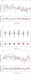 |
Fig. 2 HARPS detrended and phase-folded RV time series of TOI-396 b (top panel), TOI-396 c (middle panel), and TOI-396 d (bottom panel) with the Keplerian model superimposed in red. For each planet, the time series were obtained after subtracting the RV contribution of the other planets. The error bars also account for the jitter contribution (displayed in grey). |
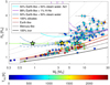 |
Fig. 3 Mass-radius diagram showing the three planets orbiting TOI- 396 (star symbol) along with the exoplanets whose density is more significant than the 3σ level (circle). All the markers are colour-coded according to the equilibrium temperature (Teq) of the planets. The thick lines are the theoretical MR BICEPS models as detailed in the legend, except for the light-blue line denoted with A21, which is taken from Aguichine et al. (2021). Earth-like means 32.5% iron + 67.5% silicates, while Mercury-like means 70% iron + 30% silicates. Models were computed for Teq = Teq,b = 1552 K (dashed-dotted lines), Teq = Teq,c = 1309 K (solid lines), and Teq = Teq,d = 1061 K (dashed lines). The difference between the A21 model and its BICEPS counterpart is due to different assumptions for e.g. pressure-temperature profiles and opacities. The dotted black lines are the iso-density loci of points corresponding to 0.5, 1, 3, 5, 10 g cm−3 (going from top to bottom). We recall that the mass estimate of TOI-396 c (the leftmost star symbol) is not statistically significant and its 3σ upper limit is |

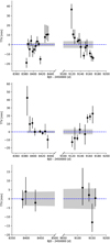 |
Fig. 4 TTV amplitudes obtained for TOI-396 b (top panel), TOI-396 c (middle panel), and TOI-396 d (bottom panel). The grey shaded region highlights the 1σ uncertainty region as derived from error propagation of the linear ephemerides. |
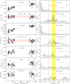 |
Fig. 5 Time series (left panels) and GLS periodograms (right panels) of the line profile variation diagnostics and activity indicators extracted from TOI-396’s HARPS spectra. In the left panels, the red curves in the first four panels mark the quadratic trends and sine functions as obtained from the best fit to the most significant peaks (false alarm probability FAP < 0.1%) identified in the corresponding GLS periodograms. In the right panels, the vertical dashed blue lines mark the orbital frequencies of the tree transiting planets. The yellow area encompasses the peaks likely due to stellar rotation. The horizontal dashed red lines mark the 0.1% false alarm probability. |
Radial velocity semi-amplitudes Kout as retrieved from MCMCI analyses of the RV time series obtained by adding an artificial Keplerian signal with period P = Pc and semi-amplitudes Kin to the original HARPS time series.
6 Joint RV and TTV dynamical analysis
As mentioned, the anti-correlation pattern of the observed TTVs (see Fig. TTVbc) is a typical signal of the dynamical interaction between TOI-396 b and c. However, the data in our hands are not enough to currently derive meaningful planetary masses from the TTVs. Indeed, the photometric observations are clustered in two groups (about two years apart), which results in a partial coverage of the curvature of the TTVs. This prevents us from accurately mapping the full phases and super-periods of the TTV signals. Hence, a dynamical fit onto the transit times would lead to a high fraction of low-amplitude TTVs with a short superperiod or to a low fraction of high-amplitude long-period TTV signals.
Despite this, we attempted to run a dynamical joint fit of the TTV and RV data set with TRADES10 (Borsato et al. 2014, 2019, 2021), a Fortran-python code developed to model TTVs and RVs simultaneously along with N-body integration. We have taken and fixed the stellar mass and radius values from Table 1. We further fixed the orbital inclinations i to the values in Table 2 and the longitude of the ascending nodes to Ω = 180°11 for all the planets. We fitted the planetary masses scaled by the stellar mass (Mb,c,d/M⋆), the orbital periods (P), the eccentricities (e) and the arguments of the pericentre (ω) in the form  , and the mean longitudes (λ12). We also fitted for an RV offset (γRV ) and for an RV jitter term (σjitter) by adopting log2 σjitter as step parameter, although we used the de-trended RV data set as derived from Section 5.2, where a jitter term was already included in the RV errors. All fitting parameters were subject to uniform priors that account for their respective physical boundaries (see Table 5); for the eccentricities we applied a log-penalty (log pe) based on the half-Gaussian (e = 0, σe = 0.083) from Van Eylen et al. (2019).
The reference time for the dynamical integration of the orbital parameters was set at Tref = 2 458 379 BJDTDB, that is before all available observations. We combined the quasi- global differential evolution (Storn & Price 1997) optimisation algorithm implemented in PYDE (Parviainen et al. 2016) with the Affine Invariant MCMC Ensemble sampler (Goodman & Weare 2010) EMCEE implemented by Foreman-Mackey et al. (2019, 2013). We first ran PYDE and evolved 68 different initial configurations of parameter sets for 50 000 generations (number of steps for which each parameter is evolved). To perform the dynamical analysis in an MCMC fashion, we then ran EMCEE, assuming as starting point the outcome obtained with PYDE. We set up 68 chains for 600 000 steps each. To sample the parameter space efficiently, we mixed the DEMove() and DESnookerMove() differential evolution moves13 in the proportion 80%–20% (Nelson et al. 2014; ter Braak & Vrugt 2008). We repeated the sequence PYDE+EMCEE twice, with different seeds for the random number generator. The chains reached convergence according to visual inspection and statistical indicators, such as the Gelman-Rubin  , the Geweke’s statistic (Geweke 1991), and the auto-correlation function14. For both runs, we applied a conservative thinning factor of 100 and discarded the first 50% of the chains (burn-in). For each run, we derived the reference outcome (hereinafter also referred to as best-fit), as the maximum-a-posteriori (MAP) parameters’ set, that is the set of parameters that maximises the log-probability15. The uncertainty of each parameter is quantified by the high- density interval (HDI) at 68.27%16 of its posterior distribution. For each parameter we computed a Z-score defined as Z-score =
  , where the subscripts denote the two different runs and ERR = HDI - MAP.
It turned out that Z-score <1 for each parameter, which allows us to merge the posterior distributions deriving from the two runs to finally compute the MAP and the respective HDI from the merged posterior distributions. We further checked the Hill stability of the system (Sundman 1913) when assuming the entire merged posterior distributions by calculating the angular momentum deficit (AMD, Laskar 1997, 2000; Laskar & Petit 2017) criterion (Eq. (26) from Petit et al. 2018). Table 5 lists the parameters returned by TRADES (MAP and HDI) along with their respective priors.
We note that the dynamical integration with TRADES allowed for a significant detection (>3σ) of the mass of TOI- 396 c, that is  . However, as explained above, TESS data do not allow. us to fully map the TTV pattern. Therefore, the present-day estimate of Mc,dyn only provides an indication of the possible mass of the planet that might not be accurate, despite its formal precision. Indeed, to accurately and reliably determine planetary masses via TTVs, it is necessary to monitor the TTV signal by benefiting of a full sampling coverage, as demonstrated for example by the cases of Kepler- 9 (Holman et al. 2010) and K2-24 (Petigura et al. 2016), whose orbital parameters and masses were comprehensively revisited by Borsato et al. (2014) and Petigura et al. (2018); Nascimbeni et al. (2024), respectively. In detail, Holman et al. (2010) had reported the masses of Kepler-9 b and c with a precision better than 8%, by performing a TTV analysis on the first three quarters of the Kepler data. Later on, by benefiting of twelve sectors of Kepler data that enabled the full mapping of the TTV phase, Borsato et al. (2014) obtained TTV-based masses differing by a factor ~ 2 from the estimate of Holman et al. (2010). Similarly, by accounting on more photometric data, Petigura et al. (2018); Nascimbeni et al. (2024) found that the mass of K2-24 c is lower by almost 2 σ than the estimate of Petigura et al. (2016) who had claimed a detection at the ~ 4 σ level.
After extracting all the synthetic transit timings Ttr (i.e. the ‘observed’: O) from TRADES’ analysis, we computed the ‘calculated’ (C) counterpart according to the linear ephemerides model based on what listed in Table 2. We plotted the O – C as a function of time as well as the RV best-fit model in Figures 6 and 7.
Additionally, we investigated if the best-fit configuration is in or close to an MMR. We integrated the MAP parameters with the N-body code REBOUND (Rein & Liu 2012) and the sym- plectic Wisdom-Holman integrator WHFAST (Rein & Tamayo 2015; Wisdom & Holman 1991) for 10 000 years. We computed the evolution of the critical resonance angles of TOI-396 b and TOI-396 c:
 (3)
(3)
where p = 3 and q = 2 (for a second order 5:3 MMR), while ϖ ≡ ω + Ω is the longitude of the pericentre. We also computed the evolution of ∆ϖ ≡ ϖb – ϖc = (ϕb – ϕc)/q. In case of MMR, we expect that both ϕb and ϕc librate (i.e. oscillate) around a fixed value for the entire orbital integration. Instead, if these angles circulate, that is they span the full 0°–360° range (or equivalently the −180°−180° range), then the planet pair is not in resonance. We found that both ϕb and ϕc circulate (see the two upper panels of Fig. 8), which indicates that the system is not in an exact 5:3 MMR. Even if ∆ϖ seems to oscillate around 0°, it circulates every ~ 2 000 years (bottom panel of Fig. 8), which further confirms that the system is not trapped in an MMR state. We also found the same behaviour for the resonant angles of 200 random samples drawn from the posterior distribution (not shown here). Our conclusions are consistent with the simulations performed by Vanderburg et al. (2019), who found that most realisations of the system are not in resonance.
As shown in Fig. 6, the MAP parameter set predicts that the TTV super-period is longer than the time spanning the two clustered TESS observations. We decided to track the potential evolution of the TTV signals over a temporal baseline of ~ 5.2 years. To this end, we ran forward numerical N-body simulations with TRADES, setting the initial conditions of the orbital parameters to be integrated at t = Tref. We ran a first simulation taking all the parameters from the MAP solution. Then, we further ran 200 simulations, where the sets of the system’s parameters were randomly drawn from the merged posterior distributions. We computed the synthetic (i.e. observed: O) transit times Ttr and created a simulated O – C plot against time, where the C counterpart of Ttr was computed assuming the linear ephemerides of Table 2. The results are displayed in Fig. 9 that emphasises a progressive drift of the O – C values inferred from the MAP parameters (black line) with respect to the zero value. As a consequence, the TTV amplitudes of planets b and c increase with time. In particular, the semi-amplitude of the O – C black curves are about two and five hours for b and c, respectively. The TTV super-period seems to be roughly equal to or larger than the integration time span, that is ∼ 5 years. The variance of the TTV amplitude (shaded area) is inferred from the results of the additional 200 simulations and reflects the widths of the posterior distributions from which the system’s parameters were drawn. The remarkable O – C drifts (i.e. the poorly constrained linear ephemerides) combined with the uncertainty on the TTV amplitudes make challenging to plan future observations of planets b and c, as the actual transit timings might differ from the linear ephemerides predictions by ∼ 5 and ∼ 10 hours for TOI-396 b and TOI-396 c, respectively. TESS will not observe the target in the foreseeable future17.
Best-fit parameters (MAP and HDI at 68.27%) along with their respective priors, as inferred from the dynamical joint modelling of RVs and TTVs with TRADES.
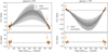 |
Fig. 6 Observed minus calculated synthetic diagrams derived from the joint RV and TTV dynamical analysis with TRADES for planet b (left panel) and c (right panel). The O – C for the best-fit (MAP) model is plotted with a black line, while the observed data points are the orange circles. The shaded grey regions displays the confidence intervals at 1, 2, and 3σ, as inferred from the 200 samples randomly drawn from the merged posterior distributions. Residuals are shown in the lower panels. |
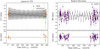 |
Fig. 7 Left panel: same as Fig. 6 but for TOI-396 d. Right panel: combined RV model of the three planets (black line) superimposed to the detrended HARPS observations (purple circles). The grey shaded area is determined from the 200 sets of system parameters randomly drawn from the merged posterior distributions as obtained from the joint dynamical analysis with TRADES. |
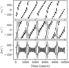 |
Fig. 8 Temporal evolution of the critical resonance angles ϕb (top panel) and ϕc (middle panel) as well as of ∆ϖ = (ϕb – ϕc)/q (bottom panel) as inferred when assuming the MAP parameters derived by the TRADES dynamical analysis and integrated with REBOUND+WHFAST for 10 000 years. |
7 Internal structure
Using the masses and transit depths reported in Table 2, we ran the neural network based internal structure modelling framework plaNETic18 (Egger et al. 2024) to infer the internal structure of TOI-396 b and d. plaNETic uses a full grid accept-reject sampling method in combination with a deep neural network (DNN) that was trained on the forward model of BICEPS (Haldemann et al. 2024) to infer the internal structure of observed planets. Each planet is modelled as a three-layered structure: an inner iron-dominated core, a silicate mantle and a fully mixed envelope made up of water and H/He. In the case of multi-planet systems, all planets are modelled simultaneously.
As modelling the internal structure of exoplanets is a highly degenerate problem, the resulting inferred structure is, at least to a certain extent, dependent on the chosen priors. To mitigate this effect, we ran a total of six models assuming six different combinations of priors. Most importantly, we use two different priors for the water content of the modelled planet, one motivated by a formation scenario outside the iceline (case A, water-rich) and one compatible with a formation inside the iceline (case B, water-poor). For both of these water priors, we choose three different options for the planetary Si/Mg/Fe ratios. In a first case, we assume that these match the stellar Si/Mg/Fe ratios exactly Thiabaud et al. (2015). Second, we assume that the planet is enriched in iron compared to its host star by using the fit of Adibekyan et al. (2021). For option 3, we model the planet independent of the stellar Si/Mg/Fe ratios, but just sampling the planetary ratios uniformly from the simplex where the molar Si, Mg and Fe ratios add up to 1, with an upper bound of 0.75 for Fe. These priors are described in more detail in Egger et al. (2024).
Figures 10 and 11 show the resulting posteriors of the most important interior structure parameters for TOI-396 b and d, respectively, in comparison with the chosen priors (dotted lines). Tables A.4 and A.5 summarise the median and one sigma error intervals for the full set of internal structure parameters. For both planets, the posterior distributions for the core and mantle mass fractions largely agree with the chosen priors for each of the six models that we ran. Indeed, the only planetary structure parameters for which the observational data contributed to their characterisation were the envelope mass fractions. If we assume that the planets formed outside the iceline, we find envelope mass fractions of  and
and  for planet b and
  and
and  for planet d, with water mass fractions in the envelope of almost 100%. Conversely, if the planets were to have formed inside the iceline, we infer envelope mass fractions of the order of 10−5 for planet b and 10−4 for planet d, almost entirely made up of H/He.
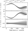 |
Fig. 9 Synthetic O – C diagrams obtained after performing forward numerical N-body simulations with TRADES (integration of 5.2 years). The C represents the timings calculated from the linear ephemerides in Table 2. The MAP model is plotted with a black line, while the confidence intervals at 1, 2, and 3σ are marked as shaded grey regions and come from 200 random samples drawn from the merged posterior distributions derived from the joint RV and TTV dynamical analysis. |
8 JWST characterisation prospects
All three planets in the TOI-396 system share similar radii (~2 R⊕), but span a wide range of masses (0.9–7.1 M⊕), which leaves open the question of whether they have primary or secondary atmospheres. Furthermore, the progression of bulk densities with distance from the host star varies in ways that cannot be described by simple formation and evolution models (e.g. Weiss et al. 2018; Mishra et al. 2023).
Given the bright host star and combination of planetary masses, radii, and equilibrium temperatures, the three planets have favourable metrics for atmospheric characterisation in both transmission and emission among sub-Neptunes (Kempton et al. 2018, see Fig. 12). This makes the TOI-396 system a highly valuable laboratory to study the formation and evolution of planetary systems. Thus, we explored the prospects for characterisation with JWST. We focused these simulations on emission observations, but we note that transmission and emission have their own advantages and disadvantages in terms of achievable science goals and challenges.
We employed the open-source PYRAT BAY modelling framework (Cubillos & Blecic 2021) to compute synthetic spectra of the TOI-396 planets. These models consist of 1D cloud- free atmospheres in radiative, thermochemical, and hydrostatic equilibrium (Cubillos et al., in prep.). We varied the models’ atmospheric elemental content to explore the wide range of compositions that the planets span. For this comparison we settled on two models to represent a primary- and a secondary-atmosphere scenario: the first is a gas giant with a 5× solar metallicity, the second is a water world with a 80% H2O plus 20% CO2 composition (based on the C/O ratios seen in the solar system minor bodies, see, e.g., Mumma & Charnley 2011; McKay et al. 2019). For the thermochemical-equilibrium calculations we considered a set of 45 neutral and ionic species, which are the main actors determining the thermal structure. For the radiative-transfer calculation we considered opacities from molecular species for CO, CO2, CH4, H2O, HCN, NH3, and C2H2 from HITEMP and EXOMOL (Rothman et al. 2010; Tennyson et al. 2016); Na and K resonant lines (Burrows et al. 2000); H, H2 , and He Rayleigh (Kurucz 1970); and H2–H2 and H2–He collision-induced absorption (Borysow et al. 2001; Borysow 2002; Richard et al. 2012). We pre-processed the large EXOMOL line lists with the REPACK algorithm (Cubillos 2017) to extract the dominant transitions. Figure 13 (top panels) shows the resulting thermal and composition structure for TOI-396 b (planets c and d follow a similar trend).
The infrared synthetic emission spectra (Fig. 13, bottom panels) are mainly shaped by H2O, CO2, and CO features. At most wavelengths the primary- and secondary-atmosphere scenarios roughly differ by an offset, which would be hard to distinguish unless the energy budget of the planets are known. In contrast, the 4–5 µm window shows the most distinctive spectral features; here the strong CO2 absorption band at 4.4 µm mainly allows one to distinguish primary from secondary atmospheres. Thus, in the following we focus on this region of the spectrum.
We simulated JWST observations using the PANDEIA exposure time calculator Pontoppidan et al. (2016). The brightness of TOI-396 limits the instrument selection to NIRCam (F444W filter) to avoid saturation. We selected the fastest readout and subarray modes, 5 groups per integration, to optimise the S/N. We generated a distribution of (noised up) realisations for each model to estimate how many eclipses are required to distinguish between primary and secondary atmospheres at the 3σ level. We found that 2, 4, and 8 eclipses (for planets b, c, and d, respectively) would be sufficient to differentiate between these two models. Figure 13 shows one of those random realisations when including the required number of eclipses. The decreasing equilibrium temperature of the planets as they are located further away from TOI-396 plays the major role in the decreasing S/N for planets c and d.
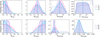 |
Fig. 10 Inferred posteriors for the most important internal structure parameters of TOI-396 b. The depicted parameters are the mass fractions of the inner core (wcore), mantle (wmantle) and envelope layers (wenvelope) with respect to the total planet mass, and the mass fraction of water in the envelope (Zenvelope). The top row shows the results when assuming a water prior motivated by a formation of the planet outside the iceline (case A), while the bottom row uses a water prior compatible with a formation inside the iceline (case B). At the same time, we run models with three different compositional priors for the planetary Si/Mg/Fe ratios: stellar (purple, option 1), iron-enriched compared to the star (pink, option 2) and sampled using a uniform prior (blue, option 3). The dotted lines show the prior distributions, while the dashed vertical lines show the median values of the posteriors. |
9 Conclusions
The object TOI-396 is an F6 V bright naked-eye star orbited by three planets of almost equal size, and the two inner planets are close to but out of a 5:3 MMR. A photometric analysis of the system was already performed by Vanderburg et al. (2019), but by benefiting from two additional TESS sectors, we improved the precision on the planet radii by a factor of ~ 1.4, obtaining  , and
, and  .
.
We determined the masses of the planets by extracting the RV time series from HARPS CCFs using an SN fit followed by a joint LC and RV MCMC analysis, where the RV de-trending uses the breakpoint method. We obtained a firm detection of the RV signals of planets b and d, deriving  and Md = 7.1 ± 1.6 M⊕, but we can provide only a 3σ upper limit for the mass of TOI-396 c of
  . This yields the following mean planet densities:
  , and
, and  , implying a quite unusual system architecture (Mishra et al. 2023) where the mid planet is the least dense and the outermost planet is the densest.
The reason for the RV non-detection of any Keplerian signal at P = Pc ~ 6 d is likely to be ascribed to the vicinity of Pc to the stellar rotation period. As a matter of fact, from the GLS periodograms of both the RV-related activity indices and the TESS raw LCs and from log R′HK-based empirical relations, we consistently inferred Prot,⋆ = 6.7 ± 1.3 d. After injecting synthetic Keplerian signals at P = Prot,⋆ and different semiamplitudes (Kin) into the RV time series, we empirically find that the RV semi-amplitudes output by the MCMC analyses (Kout) are systematically lower than the input ones by almost 3σ, and they are statistically non-significant as far as Kin ≲ Kd . In addition, we find that Kout ≈ Kc when considering a planet with Mp ~ 3 M⊕ (i.e. ρp ~ 2 g cm−3), which might correspond to the properties of TOI-396 c. On a more general perspective, these simulations confirm that stellar activity destructively interferes with Keplerian signals having P ~ Prot,⋆ (e.g. Vanderburg et al. 2016), and furthermore, they indicate that – even in the case of firm detection – values of Kout are significantly underestimated.
Longer-baseline RV observations may help disentangle coherent signals originated by Keplerian motions from noncoherent signals due to stellar activity, even if degeneracy issues still hold when the planet orbital period is close to the stellar rotation period (Kossakowski et al. 2022). Alternatively, a possible constraint on Mc may come from TTVs, as planets b and c are close to an MMR of the second order. Indeed, the TTV amplitudes of the two planets show a characteristic anti-correlation pattern, as expected; however, the phase coverage given by the available observations is too poor to perform a conclusive TTV dynamical analysis based on the observed transit timings of the planets. We also attempted to fit the TTV and RV simultaneously while integrating the orbits of the system. We found that the masses and densities of planets b and d are consistent with the results from the joint LC and RV analysis. TOI-396 c shows a dynamical mass of  , which is greater than that inferred from the joint LC and RV analysis, but it is consistent (Z-score = 1.2σ); the density is consistent at the 1.1σ level. However, we emphasise that, although formally precise, the Mc,dyn estimate might not be accurate, as the full coverage of the TTV phase is needed to reliably compute TTV-based masses. Therefore, to fully confirm the system architecture, a reliable estimate of the mass of TOI-396 c is still missing.
We also checked the evolution of the system over 10 000 years, and the critical resonance angles showed that planets b and c are close to but not in a 5:3 MMR. We further performed forward N-body simulations over a temporal baseline of ~ 5.2 years in order to track the transit epochs and evaluate the expected TTV amplitudes during time. It turns out that TOI-396 b and TOI-396 c may exhibit TTVs with a super-period of about five years and semi-amplitudes of approximately two and five hours, respectively. This translates into a temporal drift of the transit timings that can rise up to approximately five and ten hours with respect to the linear ephemerides computed from TESS data.
Studying the planetary atmospheres with JWST would take advantage of the favourable spectroscopy metrics of the system (Kempton et al. 2018). Therefore, we set up 1D cloud-free atmospheric models, generated the synthetic emission spectra of the three planets, and simulated eclipse observations with JWST. It turns out that two, four, and eight eclipses (for TOI-396 b, c, and d, respectively) would be sufficient to distinguish between primary and secondary atmosphere scenarios at the 3σ level.
Characterising the nature of the planetary atmosphere is also key to correctly assessing the planetary bulk densities (in particular for planet c). The potentially high TTVs inferred from our simulations should be duly taken into account when scheduling future observations of the target. This holds not only for JWST but also for CHEOPS (Benz et al. 2021), which appears especially suitable for collecting exquisite photometric data to enable the full characterisation of the system.
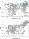 |
Fig. 12 Transit (top panel) and eclipse (bottom panel) spectroscopic metrics for the TOI-396 planets (see legend). The metrics were calculated using the 2MASS Ks-band magnitude. The grey markers show the metrics for the known sample of transiting exoplanets to date. The blue markers show the metrics for targets with approved JWST programmes. |
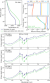 |
Fig. 13 Simulations of the atmospheric pressure profiles, eclipse spectra, and JWST observations. Top-left panel: radiative-equilibrium thermal profile of TOI-396 b assuming a gas-giant atmosphere (5× solar metallicity) and a secondary atmosphere (80% H2O plus 20% CO2). Top-right panels: volume mixing ratio of TOI-396 b for the most relevant species shaping the infrared spectrum. Bottom panels: synthetic secondary eclipse spectra of the three TOI-396 planets (solid curves). The round markers with error bars show a realisation of JWST observation with NIRCam/F444W (and their expected uncertainties) when accumulating two, four, and eight observations for planets b, c, and d, respectively. The vertical dashed lines mark the spectral window covered by NIRCam/F444W. |
Data availability
Tables A.1 to A.5 are available at the CDS via anonymous ftp to cdsarc.cds.unistra.fr (130.79.128.5) or via https://cdsarc.cds.unistra.fr/viz-bin/cat/J/A+A/693/A90. Figures A.1, A.2 are available at https://zenodo.org/records/14216673.
Acknowledgements
We thank the anonymous referee for all the valuable comments that significantly improved the quality of the manuscript. This work has made use of data from the European Space Agency (ESA) mission Gaia (https://www.cosmos.esa.int/gaia), processed by the Gaia Data Processing and Analysis Consortium (DPAC, https://www.cosmos.esa.int/web/gaia/dpac/consortium). This research made use of Lightkurve, a Python package for Kepler and TESS data analysis (Lightkurve Collaboration 2018). We thank contributors to NumPy (Harris et al. 2020), SciPy (Virtanen et al. 2020), matplotlib (Hunter 2007), astropy (Astropy Collaboration 2013, 2018, 2022), astroquery (Ginsburg et al. 2019), and tesscut (Brasseur et al. 2019). Funding for the DPAC has been provided by national institutions, in particular the institutions participating in the Gaia Multilateral Agreement. We acknowledge financial support from the Agencia Estatal de Investigación of the Ministerio de Ciencia e Innovación MCIN/AEI/10.13039/501100011033 and the ERDF “A way of making Europe” through project PID2021-125627OB-C32, and from the Centre of Excellence “Severo Ochoa” award to the Instituto de Astrofisica de Canarias. This research was funded in part by the UKRI, (Grants ST/X001121/1, EP/X027562/1). This work was supported by FCT - Fundação para a Ciência e a Tecnologia through national funds and by FEDER through COMPETE2020 - Programa Operacional Competitividade e Internacionaliza- ção by these grants: UIDB/04434/2020; UIDP/04434/2020. D.G., A.B., L.F., and L.M.S. gratefully acknowledge the financial support from the grant for internationalization (GAND_GFI_23_01) provided by the University of Turin (Italy). S.G.S acknowledges the support from FCT through Investigador FCT contract nr. CEECIND/00826/2018 and POPH/FSE (EC). P.J.W. acknowledges support from the UK Science and Technology Facilities Council (STFC) through consolidated grants ST/P000495/1, ST/T000406/1 and ST/X001121/1. N.C.S. is funded by the European Union (ERC, FIERCE, 101052347). Views and opinions expressed are however those of the author(s) only and do not necessarily reflect those of the European Union or the European Research Council. Neither the European Union nor the granting authority can be held responsible for them. J.L.-B. is funded by the MICIU/AEI/10.13039/501100011033 and NextGenerationEU/PRTR grant PID2019-107061GB-C61 and CNS2023-144309. X.D. acknowledges the support from the European Research Council (ERC) under the European Union’s Horizon 2020 research and innovation programme (grant agreement SCORE No 851555) and from the Swiss National Science Foundation under the grant SPECTRE (No 200021_215200). This work has been carried out within the framework of the NCCR PlanetS supported by the Swiss National Science Foundation under grants 51NF40_182901 and 51NF40_205606. G.N. thanks for the research funding from the Ministry of Science and Higher Education programme the “Excellence Initiative - Research University” conducted at the Centre of Excellence in Astrophysics and Astrochemistry of the Nicolaus Copernicus University in Torun´ , Poland. Research activities of the Board of Observational and Instrumental Astronomy at the Federal University of Rio Grande do Norte are supported by continuous grants from the Brazilian funding agencies CNPq. This study was financed in part by the Coordenação de Aperfeiçoamento de Pessoal de Nível Superior—Brasil (CAPES)—Finance Code 001 and CAPES-Print program. B.L.C.M., I.C.L., and J.R.M. acknowledge CNPq research fellowships. K.W.F.L. was supported by Deutsche Forschungsgemeinschaft grants RA714/14- 1, RA714/14-2 within the DFG Schwerpunkt SPP 1992, Exploring the Diversity of Extrasolar Planets. L.B. acknowledges support from CHEOPS ASI-INAF agreement n. 2019-29-HH.0. D.G. sincerely thanks Stefano Camera for the inspiring and valuable discussions on the properties of TOI-396.
References
- Addison, B., Wright, D. J., Wittenmyer, R. A., et al. 2019, PASP, 131, 115003 [NASA ADS] [CrossRef] [Google Scholar]
- Adibekyan, V. Z., Sousa, S. G., Santos, N. C., et al. 2012, A&A, 545, A32 [NASA ADS] [CrossRef] [EDP Sciences] [Google Scholar]
- Adibekyan, V., Figueira, P., Santos, N. C., et al. 2015, A&A, 583, A94 [NASA ADS] [CrossRef] [EDP Sciences] [Google Scholar]
- Adibekyan, V., Dorn, C., Sousa, S. G., et al. 2021, Science, 374, 330 [NASA ADS] [CrossRef] [Google Scholar]
- Agol, E., & Fabrycky, D. C. 2018, in Handbook of ExoplanetsURSI GASS 2020, Session J01 New Telescopes on the Frontier, eds. H. J. Deeg, & J. A. Belmonte (Cambridge University Press), 7 [Google Scholar]
- Agol, E., Steffen, J., Sari, R., & Clarkson, W. 2005, MNRAS, 359, 567 [Google Scholar]
- Aguichine, A., Mousis, O., Deleuil, M., & Marcq, E. 2021, ApJ, 914, 84 [NASA ADS] [CrossRef] [Google Scholar]
- Alexander, R. D., & Armitage, P. J. 2009, ApJ, 704, 989 [Google Scholar]
- Astropy Collaboration (Robitaille, T. P., et al.) 2013, A&A, 558, A33 [NASA ADS] [CrossRef] [EDP Sciences] [Google Scholar]
- Astropy Collaboration (Price-Whelan, A. M., et al.) 2018, AJ, 156, 123 [Google Scholar]
- Astropy Collaboration (Price-Whelan, A. M., et al.) 2022, ApJ, 935, 167 [NASA ADS] [CrossRef] [Google Scholar]
- Bai, J., & Perron, P. 2003, J. Appl. Econom., 18, 1 [CrossRef] [Google Scholar]
- Baranne, A., Queloz, D., Mayor, M., et al. 1996, A&AS, 119, 373 [NASA ADS] [CrossRef] [EDP Sciences] [Google Scholar]
- Barnes, S. A. 2010, ApJ, 722, 222 [Google Scholar]
- Benz, W., Broeg, C., Fortier, A., et al. 2021, Exp. Astron., 51, 109 [Google Scholar]
- Bergner, J. B., Öberg, K. I., Bergin, E. A., et al. 2020, ApJ, 898, 97 [NASA ADS] [CrossRef] [Google Scholar]
- Bonfanti, A., & Gillon, M. 2020, A&A, 635, A6 [NASA ADS] [CrossRef] [EDP Sciences] [Google Scholar]
- Bonfanti, A., Ortolani, S., Piotto, G., & Nascimbeni, V. 2015, A&A, 575, A18 [NASA ADS] [CrossRef] [EDP Sciences] [Google Scholar]
- Bonfanti, A., Ortolani, S., & Nascimbeni, V. 2016, A&A, 585, A5 [NASA ADS] [CrossRef] [EDP Sciences] [Google Scholar]
- Bonfanti, A., Delrez, L., Hooton, M. J., et al. 2021, A&A, 646, A157 [EDP Sciences] [Google Scholar]
- Bonfanti, A., Gandolfi, D., Egger, J. A., et al. 2023, A&A, 671, L8 [NASA ADS] [CrossRef] [EDP Sciences] [Google Scholar]
- Borsato, L., Marzari, F., Nascimbeni, V., et al. 2014, A&A, 571, A38 [NASA ADS] [CrossRef] [EDP Sciences] [Google Scholar]
- Borsato, L., Malavolta, L., Piotto, G., et al. 2019, MNRAS, 484, 3233 [NASA ADS] [CrossRef] [Google Scholar]
- Borsato, L., Piotto, G., Gandolfi, D., et al. 2021, MNRAS, 506, 3 810 [Google Scholar]
- Borsato, L., Degen, D., Leleu, A., et al. 2024, A&A, 689, A52 [NASA ADS] [CrossRef] [EDP Sciences] [Google Scholar]
- Borysow, A. 2002, A&A, 390, 779 [NASA ADS] [CrossRef] [EDP Sciences] [Google Scholar]
- Borysow, A., Jorgensen, U. G., & Fu, Y. 2001, J. Quant. Spec. Radiat. Transf., 68, 235 [NASA ADS] [CrossRef] [Google Scholar]
- Brasseur, C. E., Phillip, C., Fleming, S. W., Mullally, S. E., & White, R. L. 2019, Astrocut: Tools for creating cutouts of TESS images, Astrophysics Source Code Library [record ascl:1905.007] [Google Scholar]
- Bruntt, H., Deleuil, M., Fridlund, M., et al. 2010, A&A, 519, A51 [NASA ADS] [CrossRef] [EDP Sciences] [Google Scholar]
- Burrows, A., Marley, M. S., & Sharp, C. M. 2000, ApJ, 531, 438 [NASA ADS] [CrossRef] [Google Scholar]
- Ciardi, D. R., Fabrycky, D. C., Ford, E. B., et al. 2013, ApJ, 763, 41 [CrossRef] [Google Scholar]
- Correia, A. C. M., Delisle, J.-B., & Laskar, J. 2018, in Handbook of Exoplanets, eds. H. J. Deeg, & J. A. Belmonte (Springer International Publishing AG, part of Springer Nature), 12 [Google Scholar]
- Cubillos, P. E. 2017, ApJ, 850, 32 [CrossRef] [Google Scholar]
- Cubillos, P. E., & Blecic, J. 2021, MNRAS, 505, 2675 [NASA ADS] [CrossRef] [Google Scholar]
- Cutri, R. M., Skrutskie, M. F., van Dyk, S., et al. 2003, 2MASS All Sky Catalog of point sources. (University of Massachusetts and Infrared Processing and Analysis Center (IPAC/California Institute of Technology)) [Google Scholar]
- D’Angelo, G., & Lubow, S. H. 2008, ApJ, 685, 560 [CrossRef] [Google Scholar]
- Delisle, J. B., Laskar, J., Correia, A. C. M., & Boué, G. 2012, A&A, 546, A71 [NASA ADS] [CrossRef] [EDP Sciences] [Google Scholar]
- Delrez, L., Ehrenreich, D., Alibert, Y., et al. 2021, Nat. Astron., 5, 775 [NASA ADS] [CrossRef] [Google Scholar]
- Dorn, C., Venturini, J., Khan, A., et al. 2017, A&A, 597, A37 [NASA ADS] [CrossRef] [EDP Sciences] [Google Scholar]
- Doyle, A. P., Davies, G. R., Smalley, B., Chaplin, W. J., & Elsworth, Y. 2014, MNRAS, 444, 3592 [Google Scholar]
- Dragomir, D., Kane, S. R., Henry, G. W., et al. 2012, ApJ, 754, 37 [NASA ADS] [CrossRef] [Google Scholar]
- Dumusque, X., Santos, N. C., Udry, S., Lovis, C., & Bonfils, X. 2011a, A&A, 527, A82 [NASA ADS] [CrossRef] [EDP Sciences] [Google Scholar]
- Dumusque, X., Udry, S., Lovis, C., Santos, N. C., & Monteiro, M. J. P. F. G. 2011b, A&A, 525, A140 [NASA ADS] [CrossRef] [EDP Sciences] [Google Scholar]
- Egger, J. A., Osborn, H. P., Kubyshkina, D., et al. 2024, A&A, 688, A223 [NASA ADS] [CrossRef] [EDP Sciences] [Google Scholar]
- Espinoza, N., & Jordán, A. 2015, MNRAS, 450, 1879 [Google Scholar]
- Fabrycky, D. C., Lissauer, J. J., Ragozzine, D., et al. 2014, ApJ, 790, 146 [Google Scholar]
- Foreman-Mackey, D., Hogg, D. W., Lang, D., & Goodman, J. 2013, PASP, 125, 306 [Google Scholar]
- Foreman-Mackey, D., Farr, W., Sinha, M., et al. 2019, J. Open Source Softw., 4, 1864 [NASA ADS] [CrossRef] [Google Scholar]
- Fridlund, M., Georgieva, I. Y., Bonfanti, A., et al. 2024, A&A, 684, A12 [NASA ADS] [CrossRef] [EDP Sciences] [Google Scholar]
- Gaia Collaboration (Vallenari, A., et al.) 2023, A&A, 674, A1 [NASA ADS] [CrossRef] [EDP Sciences] [Google Scholar]
- Gandolfi, D., Barragán, O., Hatzes, A. P., et al. 2017, AJ, 154, 123 [NASA ADS] [CrossRef] [Google Scholar]
- Gardner, J. P., Mather, J. C., Clampin, M., et al. 2006, Space Sci. Rev., 123, 485 [Google Scholar]
- Gelman, A., & Rubin, D. B. 1992, Statist. Sci., 7, 457 [NASA ADS] [Google Scholar]
- Geweke, J. F. 1991, Evaluating the accuracy of sampling-based approaches to the calculation of posterior moments, Staff Report 148, Federal Reserve Bank of Minneapolis [Google Scholar]
- Ginsburg, A., Sipocz, B. M., Brasseur, C. E., et al. 2019, AJ, 157, 98 [NASA ADS] [CrossRef] [Google Scholar]
- Goldreich, P., & Tremaine, S. 1980, ApJ, 241, 425 [Google Scholar]
- Goodman, J., & Weare, J. 2010, Commun. Appl. Math. Computat. Sci., 5, 65 [Google Scholar]
- Gray, R. O., Corbally, C. J., Garrison, R. F., et al. 2006, AJ, 132, 161 [Google Scholar]
- Haldemann, J., Dorn, C., Venturini, J., Alibert, Y., & Benz, W. 2024, A&A, 681, A96 [NASA ADS] [CrossRef] [EDP Sciences] [Google Scholar]
- Handberg, R., Lund, M. N., White, T. R., et al. 2021, AJ, 162, 170 [NASA ADS] [CrossRef] [Google Scholar]
- Harris, C. R., Millman, K. J., van der Walt, S. J., et al. 2020, Nature, 585, 357 [NASA ADS] [CrossRef] [Google Scholar]
- Hatzes, A. P. 2016, in Astrophysics and Space Science Library, 428, Methods of Detecting Exoplanets: 1st Advanced School on Exoplanetary Science, eds. V. Bozza, L. Mancini, & A. Sozzetti, 3 [Google Scholar]
- Hatzes, A. P. 2019, The Doppler Method for the Detection of Exoplanets (Institute of Physics Publishing) [Google Scholar]
- Hatzes, A. P., Dvorak, R., Wuchterl, G., et al. 2010, A&A, 520, A93 [NASA ADS] [CrossRef] [EDP Sciences] [Google Scholar]
- Haywood, R. D., Collier Cameron, A., Queloz, D., et al. 2014, MNRAS, 443, 2517 [Google Scholar]
- Høg, E., Fabricius, C., Makarov, V. V., et al. 2000, A&A, 355, L27 [Google Scholar]
- Holman, M. J., Winn, J. N., Latham, D. W., et al. 2006, ApJ, 652, 1715 [NASA ADS] [CrossRef] [Google Scholar]
- Holman, M. J., Fabrycky, D. C., Ragozzine, D., et al. 2010, Science, 330, 51 [Google Scholar]
- Hunter, J. D. 2007, Comput. Sci. Eng., 9, 90 [NASA ADS] [CrossRef] [Google Scholar]
- Izidoro, A., Ogihara, M., Raymond, S. N., et al. 2017, MNRAS, 470, 1750 [Google Scholar]
- Jenkins, J. M., Twicken, J. D., McCauliff, S., et al. 2016, SPIE Conf. Ser., 9913, 99133E [Google Scholar]
- Kass, R. E., & Raftery, A. E. 1995, J. Am. Statist. Assoc., 90, 773 [CrossRef] [Google Scholar]
- Kempton, E. M. R., Bean, J. L., Louie, D. R., et al. 2018, PASP, 130, 114401 [Google Scholar]
- Kipping, D. M. 2010, MNRAS, 408, 1758 [Google Scholar]
- Kossakowski, D., Kürster, M., Henning, T., et al. 2022, A&A, 666, A143 [NASA ADS] [CrossRef] [EDP Sciences] [Google Scholar]
- Kuerster, M., Schmitt, J. H. M. M., Cutispoto, G., & Dennerl, K. 1997, A&A, 320, 831 [Google Scholar]
- Kurucz, R. L. 1970, SAO Special Report, 309 [Google Scholar]
- Kurucz, R. L. 1993, SYNTHE spectrum synthesis programs and line data (Cambridge, MA: Smithsonian Astrophysical Observatory) [Google Scholar]
- Kurucz, R. L. 2013, ATLAS12: Opacity sampling model atmosphere program [Google Scholar]
- Laskar, J. 1997, A&A, 317, L75 [NASA ADS] [Google Scholar]
- Laskar, J. 2000, Phys. Rev. Lett., 84, 3240 [Google Scholar]
- Laskar, J., & Petit, A. C. 2017, A&A, 605, A72 [NASA ADS] [CrossRef] [EDP Sciences] [Google Scholar]
- Lee, M. H., & Peale, S. J. 2002, ApJ, 567, 596 [Google Scholar]
- Leleu, A., Alibert, Y., Hara, N. C., et al. 2021, A&A, 649, A26 [NASA ADS] [CrossRef] [EDP Sciences] [Google Scholar]
- Li, M., Huang, S., Petaev, M. I., Zhu, Z., & Steffen, J. H. 2020, MNRAS, 495, 2543 [CrossRef] [Google Scholar]
- Lightkurve Collaboration (Cardoso, J. V. d. M., et al.) 2018, Lightkurve: Kepler and TESS time series analysis in Python, Astrophysics Source Code Library [record ascl:1812.013] [Google Scholar]
- Lin, D. N. C., & Papaloizou, J. 1979, MNRAS, 186, 799 [Google Scholar]
- Lindegren, L., Bastian, U., Biermann, M., et al. 2021, A&A, 649, A4 [EDP Sciences] [Google Scholar]
- Lissauer, J. J., Ragozzine, D., Fabrycky, D. C., et al. 2011, ApJS, 197, 8 [Google Scholar]
- Lovis, C., & Pepe, F. 2007, A&A, 468, 1115 [NASA ADS] [CrossRef] [EDP Sciences] [Google Scholar]
- Lund, M. N., Handberg, R., Buzasi, D. L., et al. 2021, ApJS, 257, 53 [NASA ADS] [CrossRef] [Google Scholar]
- Luque, R., Osborn, H. P., Leleu, A., et al. 2023, Nature, 623, 932 [NASA ADS] [CrossRef] [Google Scholar]
- Mamajek, E. E., & Hillenbrand, L. A. 2008, ApJ, 687, 1264 [Google Scholar]
- Marigo, P., Girardi, L., Bressan, A., et al. 2017, ApJ, 835, 77 [Google Scholar]
- Mayor, M., Pepe, F., Queloz, D., et al. 2003, The Messenger, 114, 20 [NASA ADS] [Google Scholar]
- McKay, A. J., DiSanti, M. A., Kelley, M. S. P., et al. 2019, AJ, 158, 128 [NASA ADS] [CrossRef] [Google Scholar]
- Mishra, L., Alibert, Y., Udry, S., & Mordasini, C. 2023, A&A, 670, A68 [NASA ADS] [CrossRef] [EDP Sciences] [Google Scholar]
- Morton, T. D. 2012, ApJ, 761, 6 [NASA ADS] [CrossRef] [Google Scholar]
- Morton, T. D. 2015, VESPA: False positive probabilities calculator, Astrophysics Source Code Library [record ascl:1503.011] [Google Scholar]
- Mumma, M. J., & Charnley, S. B. 2011, ARA&A, 49, 471 [NASA ADS] [CrossRef] [Google Scholar]
- Murdoch, K. A., Hearnshaw, J. B., & Clark, M. 1993, ApJ, 413, 349 [CrossRef] [Google Scholar]
- Nascimbeni, V., Borsato, L., Zingales, T., et al. 2023, A&A, 673, A42 [NASA ADS] [CrossRef] [EDP Sciences] [Google Scholar]
- Nascimbeni, V., Borsato, L., Leonardi, P., et al. 2024, A&A, 690, A349 [NASA ADS] [CrossRef] [EDP Sciences] [Google Scholar]
- Nelson, B., Ford, E. B., & Payne, M. J. 2014, ApJS, 210, 11 [Google Scholar]
- Noyes, R. W., Hartmann, L. W., Baliunas, S. L., Duncan, D. K., & Vaughan, A. H. 1984, ApJ, 279, 763 [Google Scholar]
- Otegi, J. F., Bouchy, F., & Helled, R. 2020a, A&A, 634, A43 [NASA ADS] [CrossRef] [EDP Sciences] [Google Scholar]
- Otegi, J. F., Dorn, C., Helled, R., et al. 2020b, A&A, 640, A135 [NASA ADS] [CrossRef] [EDP Sciences] [Google Scholar]
- Otegi, J. F., Helled, R., & Bouchy, F. 2022, A&A, 658, A107 [NASA ADS] [CrossRef] [EDP Sciences] [Google Scholar]
- Parviainen, H., Pallé, E., Nortmann, L., et al. 2016, A&A, 585, A114 [NASA ADS] [CrossRef] [EDP Sciences] [Google Scholar]
- Pepe, F., Mayor, M., Galland, F., et al. 2002, A&A, 388, 632 [NASA ADS] [CrossRef] [EDP Sciences] [Google Scholar]
- Perryman, M. A. C., Lindegren, L., Kovalevsky, J., et al. 1997, A&A, 323, L49 [Google Scholar]
- Persson, C. M., Fridlund, M., Barragán, O., et al. 2018, A&A, 618, A33 [NASA ADS] [CrossRef] [EDP Sciences] [Google Scholar]
- Petigura, E. A., Howard, A. W., Lopez, E. D., et al. 2016, ApJ, 818, 36 [Google Scholar]
- Petigura, E. A., Benneke, B., Batygin, K., et al. 2018, AJ, 156, 89 [Google Scholar]
- Petit, A. C., Laskar, J., & Boué, G. 2018, A&A, 617, A93 [NASA ADS] [CrossRef] [EDP Sciences] [Google Scholar]
- Piskunov, N., & Valenti, J. A. 2017, A&A, 597, A16 [NASA ADS] [CrossRef] [EDP Sciences] [Google Scholar]
- Piskunov, N. E., Kupka, F., Ryabchikova, T. A., Weiss, W. W., & Jeffery, C. S. 1995, A&AS, 112, 525 [Google Scholar]
- Pont, F., Zucker, S., & Queloz, D. 2006, MNRAS, 373, 231 [NASA ADS] [CrossRef] [Google Scholar]
- Pontoppidan, K. M., Pickering, T. E., Laidler, V. G., et al. 2016, SPIE Conf. Ser., 9910, 991016 [NASA ADS] [Google Scholar]
- Queloz, D., Henry, G. W., Sivan, J. P., et al. 2001, A&A, 379, 279 [NASA ADS] [CrossRef] [EDP Sciences] [Google Scholar]
- Rein, H., & Liu, S. F. 2012, A&A, 537, A128 [NASA ADS] [CrossRef] [EDP Sciences] [Google Scholar]
- Rein, H., & Tamayo, D. 2015, MNRAS, 452, 376 [Google Scholar]
- Richard, C., Gordon, I. E., Rothman, L. S., et al. 2012, J. Quant. Spec. Radiat. Transf., 113, 1276 [NASA ADS] [CrossRef] [Google Scholar]
- Ricker, G. R., Winn, J. N., Vanderspek, R., et al. 2015, J. Astron. Telesc. Instrum. Syst., 1, 014003 [Google Scholar]
- Rothman, L. S., Gordon, I. E., Barber, R. J., et al. 2010, J. Quant. Spec. Radiat. Transf., 111, 2139 [NASA ADS] [CrossRef] [Google Scholar]
- Santos, N. C., Sousa, S. G., Mortier, A., et al. 2013, A&A, 556, A150 [NASA ADS] [CrossRef] [EDP Sciences] [Google Scholar]
- Schwarz, G. 1978, Ann. Statist., 6, 461 [Google Scholar]
- Simola, U., Dumusque, X., & Cisewski-Kehe, J. 2019, A&A, 622, A131 [NASA ADS] [CrossRef] [EDP Sciences] [Google Scholar]
- Simola, U., Bonfanti, A., Dumusque, X., et al. 2022, A&A, 664, A127 [NASA ADS] [CrossRef] [EDP Sciences] [Google Scholar]
- Smith, J. C., Stumpe, M. C., Van Cleve, J. E., et al. 2012, PASP, 124, 1000 [Google Scholar]
- Sneden, C. A. 1973, PhD thesis, The University of Texas at Austin [Google Scholar]
- Sousa, S. G. 2014, in Determination of Atmospheric Parameters of B-, A-, F- and G-Type Stars, eds. E. Niemczura, B. Smalley, & W. Pych (Cham: Springer International Publishing), 297 [Google Scholar]
- Sousa, S. G., Santos, N. C., Israelian, G., Mayor, M., & Monteiro, M. J. P. F. G. 2007, A&A, 469, 783 [NASA ADS] [CrossRef] [EDP Sciences] [Google Scholar]
- Sousa, S. G., Santos, N. C., Mayor, M., et al. 2008, A&A, 487, 373 [NASA ADS] [CrossRef] [EDP Sciences] [Google Scholar]
- Sousa, S. G., Santos, N. C., Adibekyan, V., Delgado-Mena, E., & Israelian, G. 2015, A&A, 577, A67 [NASA ADS] [CrossRef] [EDP Sciences] [Google Scholar]
- Sousa, S. G., Adibekyan, V., Delgado-Mena, E., et al. 2021, A&A, 656, A53 [NASA ADS] [CrossRef] [EDP Sciences] [Google Scholar]
- Storn, R., & Price, K. 1997, J. Global Optim., 11, 341 [Google Scholar]
- Stumpe, M. C., Smith, J. C., Van Cleve, J. E., et al. 2012, PASP, 124, 985 [Google Scholar]
- Stumpe, M. C., Smith, J. C., Catanzarite, J. H., et al. 2014, PASP, 126, 100 [Google Scholar]
- Suárez Mascareño, A., Rebolo, R., González Hernández, J. I., & Esposito, M. 2017, MNRAS, 468, 4772 [Google Scholar]
- Sundman, K. F. 1913, Acta Math., 36, 105 [CrossRef] [Google Scholar]
- Tanaka, H., Takeuchi, T., & Ward, W. R. 2002, ApJ, 565, 1257 [Google Scholar]
- Tennyson, J., Yurchenko, S. N., Al-Refaie, A. F., et al. 2016, J. Mol. Spectrosc., 327, 73 [Google Scholar]
- ter Braak, C. J. F., & Vrugt, J. A. 2008, Statist. Comput., 18, 435 [NASA ADS] [CrossRef] [Google Scholar]
- Thiabaud, A., Marboeuf, U., Alibert, Y., et al. 2014, A&A, 562, A27 [NASA ADS] [CrossRef] [EDP Sciences] [Google Scholar]
- Thiabaud, A., Marboeuf, U., Alibert, Y., Leya, I., & Mezger, K. 2015, A&A, 574, A138 [NASA ADS] [CrossRef] [EDP Sciences] [Google Scholar]
- Trotta, R. 2007, MNRAS, 378, 72 [CrossRef] [Google Scholar]
- Van Eylen, V., Albrecht, S., Huang, X., et al. 2019, AJ, 157, 61 [Google Scholar]
- Vanderburg, A., Plavchan, P., Johnson, J. A., et al. 2016, MNRAS, 459, 3565 [NASA ADS] [CrossRef] [Google Scholar]
- Vanderburg, A., Huang, C. X., Rodriguez, J. E., et al. 2019, ApJ, 881, L19 [Google Scholar]
- Virtanen, P., Gommers, R., Oliphant, T. E., et al. 2020, Nature Methods, 17, 261 [CrossRef] [Google Scholar]
- Walsh, C., Nomura, H., & van Dishoeck, E. 2015, A&A, 582, A88 [NASA ADS] [CrossRef] [EDP Sciences] [Google Scholar]
- Weiss, L. M., & Marcy, G. W. 2014, ApJ, 783, L6 [Google Scholar]
- Weiss, L. M., Marcy, G. W., Petigura, E. A., et al. 2018, AJ, 155, 48 [Google Scholar]
- Wildi, F., Pepe, F., Chazelas, B., Lo Curto, G., & Lovis, C. 2010, SPIE Conf. Ser., 7735, 77354X [NASA ADS] [Google Scholar]
- Winn, J. N. 2010, in Exoplanets, ed. S. Seager (Tucson, AZ: University of Arizona Press), 55 [Google Scholar]
- Winn, J. N., & Fabrycky, D. C. 2015, ARA&A, 53, 409 [Google Scholar]
- Wisdom, J., & Holman, M. 1991, AJ, 102, 1528 [Google Scholar]
- Zechmeister, M., & Kürster, M. 2009, A&A, 496, 577 [CrossRef] [EDP Sciences] [Google Scholar]
The last version, ARES v2, can be downloaded at https://github.com/sousasag/ARES
Please refer to https://tasoc.dk/docs/EXP-TESS-ARC-ICD-TM-0014-Rev-F.pdf for further details about the output of the TESS science data products.
The planet properties were downloaded from the Nasa Exoplanet Archive as of 5 June 2024: https://exoplanetarchive.ipac.caltech.edu/
The spectral resolution is defined as the inverse of the time baseline. Our observations cover a baseline of about 177.4 d, which yields a spectral resolution of ∼0.0056 d−1.
Rather than assigning to the mean an uncertainty equal to the standard error, we adopted a more conservative uncertainty equal to the standard deviation of our 78 measurements.
We assumed the same reference system of Winn (2010) and Borsato et al. (2014) and later used in Borsato et al. (2019, 2021, 2024); Nascimbeni et al. (2023, 2024).
The mean longitude is defined as λ = ω + Ω + ℳ, where ω is the argument of the pericentre, Ω is the longitude of the ascending node, and ℳ is the mean anomaly.
See EMCEE documentation: https://emcee.readthedocs.io/en/stable/tutorials/moves/
See e.g. Goodman & Weare (2010) and the EMCEE documentation at https://emcee.readthedocs.io/en/stable/tutorials/autocorr/#autocorr
The log-probability is given by log 𝒫 = log ℒ + log pe, where log ℒ is the log-likelihood and log pe is the log-penalty of the eccentricities.
An HDI at 68.27% is the equivalent of the 15.87th - 84.14th percentile range of a Normal distribution that provides the 1σ standard confidence interval.
All Tables
System parameters as derived from the joint LC and RV analysis accounting for TTVs.
Radial velocity semi-amplitudes Kout as retrieved from MCMCI analyses of the RV time series obtained by adding an artificial Keplerian signal with period P = Pc and semi-amplitudes Kin to the original HARPS time series.
Best-fit parameters (MAP and HDI at 68.27%) along with their respective priors, as inferred from the dynamical joint modelling of RVs and TTVs with TRADES.
All Figures
|
Fig. 1 TESS detrended and phase-folded LCs (blue dots) of TOI-396 b (top panel), TOI-396 c (middle panel), and TOI-396 d (bottom panel) with the transit model superimposed in red. The black markers are the binned data points (binning 20 min). |
| In the text | |
|
Fig. 2 HARPS detrended and phase-folded RV time series of TOI-396 b (top panel), TOI-396 c (middle panel), and TOI-396 d (bottom panel) with the Keplerian model superimposed in red. For each planet, the time series were obtained after subtracting the RV contribution of the other planets. The error bars also account for the jitter contribution (displayed in grey). |
| In the text | |
|
Fig. 3 Mass-radius diagram showing the three planets orbiting TOI- 396 (star symbol) along with the exoplanets whose density is more significant than the 3σ level (circle). All the markers are colour-coded according to the equilibrium temperature (Teq) of the planets. The thick lines are the theoretical MR BICEPS models as detailed in the legend, except for the light-blue line denoted with A21, which is taken from Aguichine et al. (2021). Earth-like means 32.5% iron + 67.5% silicates, while Mercury-like means 70% iron + 30% silicates. Models were computed for Teq = Teq,b = 1552 K (dashed-dotted lines), Teq = Teq,c = 1309 K (solid lines), and Teq = Teq,d = 1061 K (dashed lines). The difference between the A21 model and its BICEPS counterpart is due to different assumptions for e.g. pressure-temperature profiles and opacities. The dotted black lines are the iso-density loci of points corresponding to 0.5, 1, 3, 5, 10 g cm−3 (going from top to bottom). We recall that the mass estimate of TOI-396 c (the leftmost star symbol) is not statistically significant and its 3σ upper limit is |
| In the text | |
|
Fig. 4 TTV amplitudes obtained for TOI-396 b (top panel), TOI-396 c (middle panel), and TOI-396 d (bottom panel). The grey shaded region highlights the 1σ uncertainty region as derived from error propagation of the linear ephemerides. |
| In the text | |
|
Fig. 5 Time series (left panels) and GLS periodograms (right panels) of the line profile variation diagnostics and activity indicators extracted from TOI-396’s HARPS spectra. In the left panels, the red curves in the first four panels mark the quadratic trends and sine functions as obtained from the best fit to the most significant peaks (false alarm probability FAP < 0.1%) identified in the corresponding GLS periodograms. In the right panels, the vertical dashed blue lines mark the orbital frequencies of the tree transiting planets. The yellow area encompasses the peaks likely due to stellar rotation. The horizontal dashed red lines mark the 0.1% false alarm probability. |
| In the text | |
|
Fig. 6 Observed minus calculated synthetic diagrams derived from the joint RV and TTV dynamical analysis with TRADES for planet b (left panel) and c (right panel). The O – C for the best-fit (MAP) model is plotted with a black line, while the observed data points are the orange circles. The shaded grey regions displays the confidence intervals at 1, 2, and 3σ, as inferred from the 200 samples randomly drawn from the merged posterior distributions. Residuals are shown in the lower panels. |
| In the text | |
|
Fig. 7 Left panel: same as Fig. 6 but for TOI-396 d. Right panel: combined RV model of the three planets (black line) superimposed to the detrended HARPS observations (purple circles). The grey shaded area is determined from the 200 sets of system parameters randomly drawn from the merged posterior distributions as obtained from the joint dynamical analysis with TRADES. |
| In the text | |
|
Fig. 8 Temporal evolution of the critical resonance angles ϕb (top panel) and ϕc (middle panel) as well as of ∆ϖ = (ϕb – ϕc)/q (bottom panel) as inferred when assuming the MAP parameters derived by the TRADES dynamical analysis and integrated with REBOUND+WHFAST for 10 000 years. |
| In the text | |
|
Fig. 9 Synthetic O – C diagrams obtained after performing forward numerical N-body simulations with TRADES (integration of 5.2 years). The C represents the timings calculated from the linear ephemerides in Table 2. The MAP model is plotted with a black line, while the confidence intervals at 1, 2, and 3σ are marked as shaded grey regions and come from 200 random samples drawn from the merged posterior distributions derived from the joint RV and TTV dynamical analysis. |
| In the text | |
|
Fig. 10 Inferred posteriors for the most important internal structure parameters of TOI-396 b. The depicted parameters are the mass fractions of the inner core (wcore), mantle (wmantle) and envelope layers (wenvelope) with respect to the total planet mass, and the mass fraction of water in the envelope (Zenvelope). The top row shows the results when assuming a water prior motivated by a formation of the planet outside the iceline (case A), while the bottom row uses a water prior compatible with a formation inside the iceline (case B). At the same time, we run models with three different compositional priors for the planetary Si/Mg/Fe ratios: stellar (purple, option 1), iron-enriched compared to the star (pink, option 2) and sampled using a uniform prior (blue, option 3). The dotted lines show the prior distributions, while the dashed vertical lines show the median values of the posteriors. |
| In the text | |
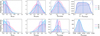 |
Fig. 11 Same as Figure 10 but for TOI-396 d. |
| In the text | |
|
Fig. 12 Transit (top panel) and eclipse (bottom panel) spectroscopic metrics for the TOI-396 planets (see legend). The metrics were calculated using the 2MASS Ks-band magnitude. The grey markers show the metrics for the known sample of transiting exoplanets to date. The blue markers show the metrics for targets with approved JWST programmes. |
| In the text | |
|
Fig. 13 Simulations of the atmospheric pressure profiles, eclipse spectra, and JWST observations. Top-left panel: radiative-equilibrium thermal profile of TOI-396 b assuming a gas-giant atmosphere (5× solar metallicity) and a secondary atmosphere (80% H2O plus 20% CO2). Top-right panels: volume mixing ratio of TOI-396 b for the most relevant species shaping the infrared spectrum. Bottom panels: synthetic secondary eclipse spectra of the three TOI-396 planets (solid curves). The round markers with error bars show a realisation of JWST observation with NIRCam/F444W (and their expected uncertainties) when accumulating two, four, and eight observations for planets b, c, and d, respectively. The vertical dashed lines mark the spectral window covered by NIRCam/F444W. |
| In the text | |
Current usage metrics show cumulative count of Article Views (full-text article views including HTML views, PDF and ePub downloads, according to the available data) and Abstracts Views on Vision4Press platform.
Data correspond to usage on the plateform after 2015. The current usage metrics is available 48-96 hours after online publication and is updated daily on week days.
Initial download of the metrics may take a while.