| Issue |
A&A
Volume 709, May 2026
|
|
|---|---|---|
| Article Number | A235 | |
| Number of page(s) | 22 | |
| Section | Interstellar and circumstellar matter | |
| DOI | https://doi.org/10.1051/0004-6361/202558615 | |
| Published online | 19 May 2026 | |
JOYS: Linking the molecular ice and gas phase composition toward the high-mass hot core IRAS 18089–1732
1
Max Planck Institute for Astronomy,
Königstuhl 17,
69117
Heidelberg,
Germany
2
Laboratory for Astrophysics, Leiden Observatory, Leiden University,
PO Box 9513,
2300 RA
Leiden,
The Netherlands
3
Leiden Observatory, Leiden University,
PO Box 9513,
2300 RA
Leiden,
The Netherlands
4
Max Planck Institut für Extraterrestrische Physik (MPE),
Giessenbachstrasse 1,
85748
Garching,
Germany
5
European Southern Observatory,
Karl-Schwarzschild-Strasse 2,
85748
Garching,
Germany
6
INAF - Osservatorio Astronomico di Capodimonte,
Salita Moiariello 16,
80131
Napoli,
Italy
7
UK Astronomy Technology Centre, Royal Observatory, Edinburgh,
Blackford Hill,
Edinburgh,
EH9 3HJ,
UK
8
Department of Physics, University of Helsinki,
PO box 64,
00014
Helsinki,
Finland
9
INAF - Osservatorio Astronomico di Roma,
Via di Frascati 33,
00078
Monte Porzio Catone,
Italy
★ Corresponding author: This email address is being protected from spambots. You need JavaScript enabled to view it.
Received:
17
December
2025
Accepted:
24
March
2026
Abstract
Context. The formation and destruction of molecules in the interstellar medium involve a complex interplay between gas phase reactions, as well as processes on grain surfaces and within icy mantles. In recent decades, the gas phase composition of the cold material toward star-forming regions could be well characterized using (sub)millimeter facilities. Prior to the launch of the James Webb Space Telescope (JWST), ice species other than the main constituents (i.e., H2O, CO, CO2, NH3, CH4, and CH3OH) were challenging to detect due to insufficient sensitivity as well as angular and/or spectral resolution.
Aims. We aim to determine molecular ice and gas phase column densities toward the young and embedded high-mass hot core IRAS 18089-1732 within a region of 5000 au.
Methods. We used spectroscopic data from 5 to 28 μm obtained with JWST to derive the ice column densities of H2O, SO2, OCN−, CH4, HCOO−, HCOOH, CH3CHO, CH3COOH, C2H5OH, CH3OCH3, and CH3COCH3. We inferred the gas phase column densities for a total of 38 molecules, including O-, N-, S-, and Si-bearing species, as well as less abundant isotopologs, from sensitive molecular line observations taken with the Atacama Large Millimeter/submillimeter Array (ALMA) at 3 mm wavelengths.
Results. We find comparable abundances (relative to C2H5OH or CH3OH) in both phases for C2H5OH, CH3OH, and CH3OCH3. The abundances of SO2 and CH3COCH3 are higher in the gas phase, suggesting additional gas phase formation routes. The abundance of CH3CHO is one order of magnitude higher in the ices compared to the gas phase. The ice abundances (relative to H2O ice) toward the IRAS 18089 hot core are similar to previously studied Galactic low- and high-mass protostars. There are hints of a decreasing abundance with galactocentric distance for OCN−, CH3OH, and CH3CHO ices.
Conclusions. It is evident that not all species show comparable abundances in the ice and gas phases. However, we do find similar trends when species show elevated ice or gas phase abundances in the high-mass hot core IRAS 18089, compared to low-mass hot cores. To better understand the reaction pathways of molecular species, statistical surveys analyzing both the ice and gas phase chemical composition of high- and low-mass protostars at different Galactocentric radii are essential.
Key words: stars: formation / stars: massive / stars: protostars / ISM: molecules
© The Authors 2026
 Open Access article, published by EDP Sciences, under the terms of the Creative Commons Attribution License (https://creativecommons.org/licenses/by/4.0), which permits unrestricted use, distribution, and reproduction in any medium, provided the original work is properly cited.
This article is published in open access under the Subscribe to Open model.
Open Access funding provided by Max Planck Society.
1 Introduction
During the earliest stages of high-mass star formation, protostars are still deeply embedded in and accreting from the surrounding cloud material (Motte et al. 2018). Within star-forming clouds, massive star formation is commonly observed toward dense clumps, with typical sizes of ∼0.1-1 pc. These clumps are often located in hub-systems, which are converging points of large-scale filaments (Kumar et al. 2020). Within a single clump, smaller cores (<0.1 pc) are embedded, where each core is expected to form either a single or small multiple system of stars (Beuther et al. 2018; Sanhueza et al. 2019; Gieser et al. 2023a; Louvet et al. 2024).
The classification of evolutionary stages during massive star formation is motivated by multiwavelength observations from infrared (IR) to radio wavelengths (Beuther et al. 2007). In particular, infrared dark clouds mark the youngest phase where the cloud is dominated by very cold gas and dust (Rathborne et al. 2006). As cores collapse and protostars reach their main accretion phase, the high-mass protostellar object (HMPO) stage is reached (van der Tak et al. 2000; Sridharan et al. 2002; Beuther et al. 2002a; Shirley et al. 2003). High luminosities and energetic outflows have been observed, along with a shift in the peak spectral energy distribution (SED) toward the mid-infrared (MIR) (Beuther et al. 2002b) indicating high accretion rates (∼10−4 M⊙ yr−1, de Wit et al. 2010; Beltrán & de Wit 2016; De Buizer et al. 2017; Lu et al. 2018). Spectra with many molecular lines are observed at (sub)millimeter (submm and mm) wavelengths toward high-mass star-forming regions (HMSFRs) when gas temperatures above 100 K are reached, due to the sublimation of molecular ices from dust grains into the gas phase (Garrod & Herbst 2006; Herbst & van Dishoeck 2009). This stage is commonly referred to as the hot (molecular) core phase (Cesaroni et al. 1997). Eventually hyper- and ultracompact H II regions end up forming due to the high UV luminosity of the central (proto)stars, which ionize and eventually disrupt the surrounding envelope material (Churchwell 2002; Dale et al. 2012; Klaassen et al. 2018).
Over recent decades, the gas phase composition toward HMSFRs obtained by sensitive radio telescope and interferometers have revealed a great complexity as a function of evolutionary stage and Galactic radius (Gerner et al. 2014; Woods et al. 2015; Coletta et al. 2020; Gieser et al. 2021; Sabatini et al. 2021; van Gelder et al. 2022; Chen et al. 2023; Bouscasse et al. 2024; Gigli et al. 2025; Nazari 2026). In contrast, only a few ice species have been detected toward HMSFRs, mostly using the Short Wavelength Spectrometer on the Infrared Space Observatory (Ehrenfreund et al. 1998; Dartois et al. 1999; Schutte et al. 1999; Gibb et al. 2000, 2004; Boogert et al. 2015, 2022). Previous ice studies toward HMSFRs were limited by poor angular resolution, sensitivity and/or spectral resolution. As a result, detailed investigations of the ice composition toward individual protostellar cores have been lacking. Based on the gas phase inventory of HMSFRs, chemical models predict that grain-surface chemistry on dust grains is important for the formation of complex organic molecules (COMs; Garrod & Herbst 2006; Herbst & van Dishoeck 2009).
Thus far, any direct comparisons between gas phase and ice abundances have only been carried out toward a small number of low-mass protostars (Perotti et al. 2021; Chen et al. 2024). It is therefore crucial to also study high-mass protostars that evolve on shorter timescales, are embedded in clustered regions, and heat up their surrounding envelope material. In addition, they have the potential to heavily influence the chemical properties of the molecular gas. Studying these environments is important since most stars form in dynamically active HMSFRs, as opposed to the nearby isolated low-mass star-forming regions.
With the launch of the James Webb Space Telescope (JWST), more sensitive observations at higher spectral and spatial resolution in the MIR have enabled more detailed characterizations of interstellar ices (Yang et al. 2022; McClure et al. 2023; Rocha et al. 2024; Chen et al. 2024; Nazari et al. 2024; Slavicinska et al. 2024; Brunken et al. 2024; Slavicinska et al. 2025; Nakibov et al. 2025; Smith et al. 2025; Rocha et al. 2025; Rayalacheruvu et al. 2025; Sewiło et al. 2025; Tyagi et al. 2025; Gross et al. 2026). Most importantly, the detection of COMs other than CH3OH can now be achieved (Rocha et al. 2024). While most of the evolved high-mass protostars in the Milky Way are too bright for JWST instruments, deeply embedded HMPOs can still be targeted thanks to their high IR extinction.
The JWST Observations of Young protoStars (JOYS) program (PI: E. F. van Dishoeck) targets a sample of low- and high-mass protostars using the Mid Infrared Instrument and Medium resolution Spectrograph (MIRI-MRS) and providing spectroscopic information from 5 to 28 μm. An overview of the observations and science results is presented in van Dishoeck et al. (2025). These MIR observations of star-forming regions with JWST allow for a detailed analysis of atomic, ionic, and molecular gas phase lines as well as molecular ices (van Dishoeck et al. 2025).
IRAS 18089-1732 (also commonly referred to as G12.89+0.49, but here we use IRAS 18089) is a HMSFR in the HMPO stage at a distance of 2.5 ± 0.3 kpc (vLSR = 33.8 km s−1) (Urquhart et al. 2018). The clump mass and bolometric luminosity are estimated to be 103.1 M⊙ and 104.3 L⊙, respectively (Urquhart et al. 2018). For a multiwavelength overview from large to small scales in the region, we refer to Appendix B in Gieser et al. (2023a).
Figure 1 presents an overview of the hot core region of IRAS 18089. The region is associated with CH3OH maser emission (Beuther et al. 2004), which shows variability with a stable period, suggesting the presence of a binary (Goedhart et al. 2009). Both the dust continuum and magnetic field morphology exhibit spiral-like structures toward the central core (Sanhueza et al. 2021). High-resolution (<0.1″) data taken with the Atacama Large Millimeter/submillimeter Array (ALMA) show disk-like kinematics that cannot be explained by a simple Keplerian rotation model (Ginsburg et al. 2023). The disk-like rotation is roughly perpendicular to the north-south directed molecular outflow oriented near the plane of sky (Beuther et al. 2004). The 3 mm ALMA continuum reveals several cores surrounding the central hot core and a Spitzer 4.5 μm point source is detected in the vicinity of the central source (Gieser et al. 2023a).
In the central region of the main core, the temperature exceeds 100 K within a radius of 10 000 au and a steep temperature profile (T ~ r-q) with q=0.8±0.1 is inferred from CH3CN line emission (Gieser et al. 2023a). At temperatures above 100 K most COMs that were frozen on the icy grains sublimate into the gas phase (Garrod et al. 2022). Therefore, IRAS 18089, targeted both by sensitive JWST (van Dishoeck et al. 2025) and ALMA (Gieser et al. 2023a) observations, is the ideal hot core source for studying the chemical inventory in the ices, as well as in the gas phase, to achieve a better understanding of COM formation processes in HMSFRs. The ice composition toward the MIR source of IRAS 18089 (Fig. 1) was analyzed in van Dishoeck et al. (2025). However, it is only at the hot core position (IRAS 18089 mm) that both the ice and gas phase can be directly compared using datasets at similar spatial resolutions.
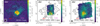 |
Fig. 1 IRAS 18089 continuum images (left: ALMA 3 mm; center: JWST/MIRI-MRS 5 μm; right: JWST/MIRI-MRS 19 μm). In all panels, the black contours show the ALMA 3 mm continuum with steps from 5, 10, 20, 40, 80, 160, and 320×σcont. The mm and MIR continuum peak positions are labeled and highlighted in red and pink. The red circle shows the aperture (1" radius) used for spectra extraction toward the mm source. A scale bar in the top left panel marks a spatial scale of 5000 au. The ellipse in the bottom left corner highlights the angular resolution of each dataset. |
2 Observations
In the following, we describe the reduction of spectroscopic data of IRAS 18089 in the MIR (5-28 μm) obtained with JWST in Sect. 2.1. We describe the reduction at 3 mm wavelengths (86.3110.3 GHz) using ALMA in Sect. 2.2.
2.1 JWST/MIRI-MRS
The observations with JWST (Gardner et al. 2023; Rigby et al. 2023) are part of the JOYS program (program ID: 1290, PI: E. F. van Dishoeck). IRAS 18089 was observed on September 18, 2023 using the MRS mode of the MIRI instrument (Rieke et al. 2015; Wright et al. 2023) in two consecutive mosaic pointings, as well as a nearby dedicated background pointing (αJ2000=18:11:44.1236 and δJ2000=-17:31:3.10). The observations included all three grating settings (short, medium, and long) and all channels (ch1, ch2, ch3, and ch4) providing a total of 12 sub-bands covering a wavelength range from 4.9 to 28 μm. The on-source time was 200 s per grating setting and per pointing. We used the two-point dither mode that is appropriate for extended sources and the default readout mode FASTR1. Due to spatial and spectral undersampling, small amplitude modulations can be present in extracted MIRI-MRS spectra when using a two-point instead of a four-point dither (Fig. 9 in Law et al. 2023). However, since our aperture for spectral extraction is large (Sect. 2.3), our data quality was not affected by this effect. The dedicated background observation was taken in the same setup with the same integration time. Strong emission lines were masked before background subtraction. A detailed description of the JOYS data reduction pipeline is presented in van Gelder et al. (2024a). The IRAS 18089 MIRI-MRS data were calibrated using the same pipeline version (1.13.4, Bushouse et al. 2024) and reference context (jwst_1188.pmap).
The final IRAS 18089 data products consist of one data cube per sub-band including the combined two-pointing mosaic. The angular resolution, θ, and spectral resolving power (R = λ∕ ∆λ) range from 0.2" to 0.8" and 4000 to 1500 from 5 to 28 μm, respectively (Argyriou et al. 2023; Jones et al. 2023; Law et al. 2023). The 5.2 μm and 19 μm continuum maps (Fig. 1) were estimated between 5.2-5.3 (ch1 short) and 19.o-19.1 μm (ch4 short) covering wavelength ranges that are absent of strong line emission or absorption.
2.2 ALMA Band 3
The ALMA observations of IRAS 18089 were carried out in Cycle 6 at 3 mm wavelengths (project code: 2018.1.00424.S, PI: C. Gieser). A detailed description of the data reduction and imaging procedure is presented in Sect. 3 and Appendix A in Gieser et al. (2023a). In this work, we used the 3 mm continuum as well as the spectral line data of in total 23 spectral windows (spws) covered by two receiver tunings covering different spectral ranges (SPRs, referred to here as SPR1 and SPR2).
The ALMA 3 mm continuum data presented in Gieser et al. (2023a) were created by combining continuum channel ranges in the entire 3 mm dataset. The noise level of the 3 mm continuum is σcont=0.057 mJy beam−1 and the synthesized beam (θmaj × θmin) is 0.79″ × 0.70″ with a position angle (PA) of 101°. The observational setup of the spectral windows is summarized in Table A.1. Depending on the spectral setup and frequency, the angular resolution of the spws vary from ≈0.6″ to ≈1.9″. The three broadband spws have a channel width of 0.977 MHz (≈3.4kms−1), while the remaining narrowband spws have a channel width of 0.244MHz (≈0.9 km s−1). The line sensitivity is ≈0.8 K and ≈0.1 K per channel in the high and low spectral resolution cubes, respectively.
2.3 Spectra extraction
An overview of the ALMA 3 mm and JWST 5.2 and 19 μm continuum data is presented in Fig. 1. The central core of IRAS 18089 (labeled “mm”) is embedded in an extended dusty envelope revealed by the 3 mm continuum. There is no significant contribution from free-free emission at this wavelength (less than 1 mJy, Zapata et al. 2006; Gieser et al. 2023a). Extended emission is also detected in both MIR continuum maps which is in contrast to the JOYS high-mass target IRAS 23385 that is also in the HMPO phase where only two point sources were detected at 5 μm (Beuther et al. 2023; Gieser et al. 2023b). The brightest source at 5.2 μm is located ≈3″ toward the southwest of the mm core, referred to as the MIR source in the following. Based on the presence of one Gaia source in the parallel 15 μm MIRI image, the astrometric correction would be less than 0.1″ and, thus, no astrometric correction was applied (Appendix B in Reyes-Reyes et al. 2026). Therefore, the offset between the mm and MIR peak is clearly due to the presence of several sources where some still remain highly embedded. We note the increase of the field of view in the MIRI-MRS data from short to long wavelengths in Fig. 1.
The 19 μm peak emission is slightly offset from both the mm and MIR peak position (0.9″ toward the southeast), which might be an effect of high extinction or the presence of more embedded sources. This position also corresponds to the emission peak at longer wavelengths (up to 28 μm) in the MIRI-MRS data. In this work, we focus on the chemical properties toward the position of the 3 mm continuum peak position, which is the hot core region. Spectra were extracted from both the JWST and ALMA data at the position of the 3 mm continuum peak at α(J2000)=18h11m51.46s and δ(J2000)= -17°31′28.75″. In both datasets, the aperture is set to a fixed radius of 1″ (red circle in Fig. 1) covering a diameter of 5000 au at the distance of IRAS 18089 (2.5 kpc). Figure 1 also shows the position of the MIR peak position, α(J2000)=18h11m51.40s and δ(J2000)= -17°31′29.96″, analyzed in van Dishoeck et al. (2025). In contrast to the hot core region, the MIR source is not associated with bright gas phase molecular line emission in the ALMA data (Sect. 3.2). Hence, this MIR source is an ideal local background source for an ice composition comparison slightly offset from the hot core region.
For each sub-band in the JWST data, we applied a 1D residual fringe correction using fit_residual_fringes_1d of the jwst python package (Kavanagh et al., in preparation). Following the method by van Gelder et al. (2024a), individual spectra from the 12 sub-bands of the JWST/MIRI-MRS data are stitched to a full spectrum from 4.9 to 26μm with small additive offsets being corrected for in each sub-band starting at the lowest wavelength data (ch1 short). We chose “ch1 short” as the reference since the photometric calibration is most accurate in this subband (Argyriou et al. 2023). The noise from ch1 to ch3 is ≈1 mJy and increases to 5, 32, 150 mJy in ch4 short, medium, and long, respectively. Given the high MIR-brightness of IRAS 18089, a high signal-to-noise ratio (S/N) ranging from 50 up to 850, was achieved.
The observed MIR spectrum of IRAS 18089 is presented in Fig. 2. The source spectrum has a large dynamic range covering four orders of magnitude. The lowest flux density is reached at ≈1 mJy at 9-11 μm due to strong silicate absorption, which is broad and flat between 9 and 11 μm once the noise threshold has been reached. The SED then rises toward longer wavelengths to 10 Jy at 26 μm, as expected from a young embedded protostar. The spectrum shows broad absorption features by molecular ices. The extraction of column densities of ice species is further explained in Sect. 3.1.
To estimate the molecular column densities of gas phase species, we extracted the mean spectrum within the same aperture size from all ALMA spws. The noise σline per channel, estimated in the 1″ radius extracted spectrum (Sect. 2.3), is ≈0.3K and ≈0.06K in the narrowband and broadband spws, respectively (Table A.1). In Sect. 3.2 we derive molecular column densities detected within this dataset.
 |
Fig. 2 JWST/MIRI-MRS spectrum of IRAS 18089 mm. The observed MIR spectrum of the mm source is shown in black. The red line is the best-fit SED model taking into account emission by two black bodies (T1 = 410 K and T2 = 83 K) and absorption by dust and water ice. The data points that were included in the fit are highlighted by the blue dots. The green line shows the contribution by dust absorption and the purple line highlights the two black body emission components. Silicate features as well as main ice constituents (Whittet et al. 1996; Gibb et al. 2000; Yang et al. 2022; McClure et al. 2023) are labeled. The wavelength range with an increased noise (8.8-11.0 μm) is shaded in gray. |
3 Results
The high-mass hot core IRAS 18089 is expected to show a rich molecular composition both in the solid state as well as the gas phase. The MIR continuum SED of IRAS 18089 and molecular constituents in the icy mantles around dust grains are analyzed in Sect. 3.1 using sensitive MIRI-MRS observations obtained with JWST. gas phase molecules are characterized in Sect. 3.2 using ALMA observations at 3 mm.
3.1 Ice column density determination using JWST MIRI-MRS spectra
Figure 2 presents the full MIRI-MRS spectrum of the IRAS 18089 mm hot core exhibiting a number of distinct absorption features. The broad and deep absorption feature at 10 μm is due to silicates and the observed flat profile at the peak absorption is due to reaching the noise floor between ≈9 μm and 11 μm (≈1 mJy). In addition to silicates, broad absorption features due to molecular ices being present in the NIR and MIR range. The molecular column densities of such ice species can be quantified by fitting the ice optical depth spectrum, τν, with reference laboratory spectra of pure ices as well as ice mixtures.
To obtain the ice optical depth spectrum, the spectral energy distribution (SED) of the continuum has to be first determined from the MIRI-MRS data (Fig. 2). The continuum SED can be estimated, for example, by interpolating guiding points set above the observed spectrum and with an additional absorption component of silicate dust τsil (Chen et al. 2024; Rocha et al. 2024; Rayalacheruvu et al. 2025). Here, we used a physically motivated approach (similar to the MIR source analysis, van Dishoeck et al. 2025) and model the continuum SED by considering black bodies Bν(T), with Fν = ΩBν(T) and emitting area Ω and by taking into account absorption by carbonaceous and silicate dust as well as H2O ice.
The dust composition is a mixture of amorphous carbon and amorphous silicates (Pollack et al. 1994). In this work, for the silicate composition, we considered the most common contributors, namely, olivine (MgFeSiO4) and pyroxene (Mg0.7Fe0.3SiO3) via
 (1)
(1)
We used the reference opacity spectra (κoli and κpyr in cm2 g−1) created with OpTool (Dominik et al. 2021), using a grain size distribution from 0.1 to 1 μm and taking into account amorphous carbon (with a volume fraction of 15%), following the same approach as for the MIR source in IRAS 18089 (see Appendix F in van Dishoeck et al. 2025). The scaling factors foli and fpyr were used to measure the average mass surface density (in g cm−2) of each dust component within the aperture.
The absorption by water ice, τH2O, was also included in our SED model. This enables a direct fit of the SED model function to the observed spectrum between 10 and 15 μm (Fig. 2). Following the analysis approach of the HMSFR IRAS 23385 MIRI-MRS spectrum (Rocha et al. 2024), the water ice composition is a combination of two temperature components at 15 and 75 K,
 (2)
(2)
The laboratory water ice optical depth spectra measured at 15 and 75 K (τH2O,15 K and τH2O,75 K) were taken from Öberg et al. (2007) with scaling factors of f1,H2O and f2,H2O, respectively, which consider different ratios of the two temperature components. To avoid over-fitting the spectrum with a model that contains too many free parameters, we iteratively started with one black body absorbed by dust and water which was not sufficient to explain the full complexity of the observed spectrum. Two black bodies with a hot and warm temperature component (T1 and T2) absorbed by dust and water were required to explain the full MIR spectrum of IRAS 18089.
We note that in reality, IRAS 18089 has a more complex temperature structure, which is a temperature gradient as a function of radius (Gieser et al. 2023a). A full radiative transfer model, including the protostar, disk and envelope components, is beyond the scope of this work. Our SED model is sufficient to determine the continuum SED which is necessary to infer the H2O ice column density that is overlapping with the silicate absorption feature at 10 μm (Fig. 2). The presence of the two black bodies at warm and hot temperatures can either indicate an underlying temperature gradient and/or two unresolved sources, which can also be expected in clustered HMSFRs. The complete SED model function, Fν,model, is

This includes a total of eight free parameters: four for the two black body components and four for the scaling factors of the dust and water reference spectra. We used the curve_fit function of the scipy python package (Gommers et al. 2024) and the emcee package (Foreman-Mackey et al. 2013) to find the best fit to the observed spectrum and estimate the uncertainties using the Markov chain Monte Carlo (MCMC) method. Given that the spectrum contains broad ice absorption features by species other than water ice and silicates (Fig. 2), we only selected specific wavelength ranges outside these ice bands for the fit (marked in Fig. 2). The lower boundary for the dust and water fit parameters (foli,fpyr,f1,H2O,f2,H2O) was set to 0; hence, the individual contributions can be 0 and do not necessarily need to be present in the fit. Additional major ice constituents present in the MIR are labeled in Fig. 2 (based on Whittet et al. 1996; Gibb et al. 2000; Yang et al. 2022; McClure et al. 2023). In addition there is a broad feature at 11.3 μm caused by polycyclic aromatic hydrocarbon (PAH) emission. There is a potential broad absorption feature at 16.3 μm that could be explained by the presence of crystalline silicates. A more detailed study of the dust composition toward IRAS 18089 is however beyond the scope of this work.
The best-fit SED model, taking into account the continuum emission and absorption by dust and water, is shown in Fig. 2 and the best-fit parameters are summarized in Table 1. The best-fit values of the MCMC SED fit were estimated from the 50th percentile and the -σ and +σ uncertainties were computed from the difference to the 16th and 84th percentiles, respectively. Overall, there is a good agreement with the observed spectrum of IRAS 18089. As expected from an embedded protostar, the black body components of the hot and warm component are ≈410 and 80 K, respectively. These components are possibly tracing the inner dusty disk and the outer disk envelope. The hot temperature component of IRAS 18089 mm is in agreement with the nearby brighter (at 5 μm) MIR source being slightly hotter (≈700 K, van Dishoeck et al. 2025). The MCMC corner plot is presented in Fig. B.1, highlighting degeneracies between the temperature and emitting area of each black body component. There are also degeneracies seen between the two silicate components as well as the two temperature components of the H2O ice.
The best-fit water composition is a mixture of 15 and 75 K indicating different temperature regimes along the line of sight. The total water column density, N(H2O), is (1.5±0.75)×1019 cm−2 (see Eq. (5)). The column densities of the cold (15 K) and warm (75 K) water component contribute 12% and 88% to the total column density. For the high-mass binary IRAS 23385, the contribution of the warm component was less (only ≈30%, Rocha et al. 2024). Full SED models of all other high-mass JOYS sources are presented in Reyes-Reyes et al. (2026) where overall the cold component dominates the modeled SEDs. Given the extended hot core region of the IRAS 18089 mm source (Gieser et al. 2023a), a significant contribution of warm water ice is expected.
The silicate absorption features at 10 and 17 μm are slightly overestimated in the SED model, due to reaching the noise limit in this regime in the MIRI-MRS data that is causing the flat profile at the bottom of the 10 μm silicate feature. A large portion of the blue part of the 10 μm silicate feature cannot be explained by the silicate composition of the best-fit model. We tried improving the fit by including an additional data point at 7.82 μm (Fig. B.2). While this does improve the fit at the blue part of the 10 μm silicate absorption, the temperature of the hot component is extreme (T1 = 1 600 K). The resulting H2O column density is 50% less compared to the best-fit SED model (Table 1). Given the uncertainties in fitting the 10 μm silicate feature, we assume therefore that the H2O ice column density is uncertain by 50%.
One explanation for the mismatch in 8-10 μm regime could be that this region contains a large amount of ice absorption and/or that the dust model is not accurate enough for a complex source such as the mm peak of IRAS 18089. There could also be an additional contribution of silicate emission originating from the pseudo disk as observed toward irradiated disks in the HMSFR NGC 6357 (Ramírez-Tannus et al. 2025). While the observed spectrum toward the 10 μm silicate feature is affected by the noise floor, this is not the case for the 17 μm feature that is however also overestimated by our SED model. At these longer MIR wavelengths, the continuum emission is extended (Fig. 1) and, hence, the environment emission contributes to the observed SED which is not taken into account in our SED model that only considers the source SED itself. This mismatch can also be explained by the dust composition toward the IRAS 18089 hot core consisting of more than a simple mixture of amorphous carbonaceous material and silicates. Since the main focus of this work is to analyze the ice composition of COMs between 6.5 and 9 μm, our best-fit SED model is sufficient to obtain an estimate of the total water column density. But future work requires a more detailed investigation of the dust properties in MIRI-MRS spectra toward low- and high-mass protostars.
The optical depth spectrum, taking into account the continuum SED with contributions from dust and water, is
 (3)
(3)
with the observed MIRI-MRS spectrum Fv,obs and Fν,model obtained from the best-fit continuum SED model including absorption by dust and water (Table 1). The optical depth spectrum in the range from 6.5 to 9.0 μm is presented in the bottom panel in Fig. 3.
To analyze the optical depth spectrum toward the range where many COM ices are present (i.e., COM region, ≈6.6-9.0 μm), a local continuum has to be first determined that removes contributions of the bulk ice features (i.e., the C-H stretch and OH-stretch at ≈6 and ≈7 μm; see Fig. 2). The MIR spectrum of IRAS 18089 shows not only deep ice absorption features, but also a plethora of gas phase lines, including CH4 in absorption and SO2 in emission. These two species have strong transitions in the COM range from ≈7.2-7.7 μm. In particular, the presence of SO2 gas phase lines in emission create a pseudo-continuum that can cancel out ice absorption (van Gelder et al. 2024b).
The CH4 and SO2 spectra were created using slab models assuming local thermal equilibrium (LTE) conditions (van Gelder et al. 2024a; Francis et al. 2024). The line width was assumed to be 4.7 km s−1 to be consistent with the slab modeling approach of the high-mass JOYS target IRAS 23385 (Francis et al. 2024). This value is based on typical LTE models of T Tauri disks (Salyk et al. 2011) and is in agreement with an average line width of ≈5 km s−1 measured for the gas phase species with ALMA (Sect. 3.2). The gas temperature was fixed to 150 K and for the SO2 slab model, we fixed the emitting radius to 100 au. We followed a similar approach to that performed for the ice analysis of the entire low-mass JOYS sample by Chen et al. (in prep.) to remove the contribution of CH4 and SO2 gas phase lines in the spectrum. We manually varied the column density of each species until (based on a visual inspection of the observed IRAS 18089 spectrum, after subtracting the slab model spectra) the gas phase line contributions were removed. We note that we have not properly fitted the gas phase species, so we refrain from further interpreting the results from the slab modeling here, as this would require a proper exploration of the parameter space (emitting radius, gas temperature, and column density). In the top panel in Fig. 3, we present the comparison before and after gas phase CH4 and SO2 removal. Both ice absorption bands at 7.3 and 7.4 μm become deeper after the correction. The importance of removing gas phase contributions before analyzing the ices is further demonstrated in Appendix E.
We then interpolated the local continuum in the optical depth spectrum toward the COM region using a set of guiding points and spline functions (Fig. 3). While in previous works, the guiding points were often placed above the observed optical depth spectrum, we have aimed to stay as close as possible to the observed spectrum to extract only the most reliable absorption features of minor ice constituents. The resulting column densities might hence be slightly underestimated. Gross et al. (2026) analyzed the ices toward a sample of low-mass protostars using MIRI-MRS data and found that the choice of the local continuum baseline does affect the derived SO2 ice column density which we further investigate in Appendix E in the case of the IRAS 18089 hot core. The final CH4 and SO2 gas phase and local continuum subtracted optical depth spectrum is presented in Fig. 4. This spectrum reveals that within the broad and deep bulk ice absorption features, there is an additional contribution of minor ices, most notably the 7.7 μm absorption by CH4.
We followed the approach by Chen et al. (2024) to determine the ice column densities. We assumed that the observed optical depth spectrum consists of a linear combination of different ice mixtures or pure ices taken from laboratory reference data,  , scaled by a factor of αm,
 (4)
(4)
A list of all considered ices (in total 12 different molecules motivated by JWST ice studies by Rocha et al. 2024; Chen et al. 2024; Rayalacheruvu et al. 2025; Sewiło et al. 2025) is summarized in Table C.1. This includes simple species (OCN−, SO2, CH4) and COMs analyzed in previous studies (Rocha et al. 2024; Chen et al. 2024; Rayalacheruvu et al. 2025; Sewiło et al. 2025). Regarding the OCN− ice, in previous studies (Rocha et al. 2024; Chen et al. 2024; Sewiło et al. 2025) only the 2ν2 band at 1295 cm−1 (7.72 μm), but not the ν1 band at 1210 cm−1 (8.26 μm) based on laboratory work by Novozamsky et al. (2001) and Raunier et al. (2003) was considered, whereas here we take into account both ice bands (Fig. C.1). The strong ν3 band of OCN−at 4.64 μm (2155 cm−1) is not covered by the MIRI-MRS data and NIRSpec observations toward this source are currently not available.
Depending on the ice mixture composition, mixing ratio, and temperature, individual ice bands can change in position and shape. For many ice species, there are only limited experimental data available, with often H2O as the bulk component measured at low temperatures (≤15 K). Chen et al. (2024) performed detailed tests on CH3CHO and found that the mixture with H2O at low temperature (15 K) provides the best match between the laboratory work and observations (their Fig. 6). For most species, we use ice mixtures with water ice as the bulk component, if available in public databases, which is the most abundant ice component. In the case of SO2 ice, only mixtures with CH3OH were available. For H2CO only pure ice spectra are available. For HCOOH it was easier to isolate HCOOH ice bands in the pure ice spectrum and similar in the case of CH3OCHO using data from the CO mixture. Isolating the ice components from the bulk component(s) is important in our ice fitting approach to reliably estimate individual contributions. However future work requires measurements of ice mixtures containing many ice components, constrained by current JWST observations, which will enable a detailed analysis of how the absorption features agree or disagree compared to simple mixtures. The laboratory spectra of ice mixtures contain contributions from, for example, H2O or CH3OH in the 6.5-9.0 μm wavelength range. In other cases, the spectra are slightly offset from zero in ranges with no ice absorption. Hence, we first applied a baseline correction to the laboratory spectra and to isolate the ice features of the minor ice constituents. Figure C.1 shows the laboratory spectra before and after baseline correction. The best-fit and uncertainties considering all ice constituents listed in Table C.1 were determined based on a least squares optimization using the curve_fit package. To avoid biasing the results, the lower boundary for the scaling factors αm was set to 0; hence, in the fittings, the individual ice constituents were not forced to be present.
The ice column density is then calculated using the band strength A of specific ice bands and integrating the best-fit scaled laboratory optical depth spectrum over the ice feature (in wave numbers ν̃), expressed as
 (5)
(5)
Table C.1 summarizes the considered molecules and their band strengths. For most ice bands (except for H2O and OCN−), we use the same band strength values as in Chen et al. (2024). Mastrapa et al. (2009) measured band strengths for amorphous water ice within a range of 2.5 × 10⁻¹⁷ cm molecule−1 to 3.0 × 10⁻¹⁷ cm molecule−1 between 15 K and 80 K. For H2O we use an average of 2.8 × 10⁻¹⁷ cm molecule−1 (Mastrapa et al. 2009), compared to 3.2 × 10⁻¹⁷ cm molecule−1 used in Chen et al. (2024) and Rocha et al. (2024). Rocha et al. (2024) calculated the OCN− band strength of the 7.72 μm ice band (A7.7 = 7.5 × 10⁻¹⁸ cm molecule−1) based on the 4.6 μm band (A4.6 = 1.3 × 10⁻¹⁶ cm molecule−1, van Broekhuizen et al. 2005). Here, we use recent measurements on the 4.6 μm band strength (A4.6 = 1.51 × 10⁻¹⁶ cm molecule−1, Gerakines et al. 2025) and following the extrapolation by Rocha et al. (2024) estimate A = 8.7 × 10⁻¹⁸ cm molecule−1 for the 7.72 μm ice band strength.
The best-fit ice optical depth spectrum is presented in Fig. 4, where all individual ices are highlighted as well. Out of the 12 ice species included in the fitting, we find that ten of them are present in the spectrum of IRAS 18089 mm. We find no evidence of significant H2CO and CH3OCHO ice contributions to the observed spectrum with both scaling factors best-fitted with αm = 0. Hence we refrain from reporting upper limits for those species. The ice column density uncertainties are calculated including the uncertainties obtained from the fit and an additional 20% to take into account any uncertainties on the local continuum determination and ice band strength. In Appendix E, we present additional tests of our ice fitting method. One caveat in this ice fitting approach is that all results are based on the assumption that no other ice constituents are present in the spectrum.
The main constituents are CH4, OCN− and HCOO− ices (τmax>0.1). Minor contributors (τmax between 0.01 and 0.1) are SO2, CH3CHO, CH3OCH3, CH3COOH, HCOOH, CH3COCH3, and C2H5OH ices. The strong absorption feature at 8.35 μm that was also detected in the MIR source of IRAS 18089 (van Dishoeck et al. 2025) remains unidentified using public ice laboratory reference spectra. It is however likely originating from a CH2OH band measured at 1197 cm−1 (corresponding to 8.35 μm) occurring when CH3OH is exposed to UV irradiation (Öberg et al. 2009; Yocum et al. 2021). There is also an absorption feature of NH2OH ice measured in laboratory experiments (1191 cm−1, Nightingale & Wagner 1954) and (1201 cm−1, Zheng & Kaiser 2010) corresponding to the NH2 rocking mode that is close to the unidentified observed absorption feature. However, the NOH bending mode measured at 1515 (6.6 μm) and 1486 cm−1 (6.73 μm) by these experimental works, respectively, is not observed toward IRAS 18089. Nevertheless we cannot fully exclude the possibility that NH2-group containing ice species might be contributing to this feature. The absorption band at 7.2 μm can be only partially (≈60%) explained by a combination of HCOO−, CH3COOH, and C2H5OH ice. Small offsets of the best-fit compared to the observed spectrum are likely linked to the local continuum estimate (Fig. 3).
The derived ice column densities, including H2O from the SED model fit (Sect. 3.1), are summarized in Table D.1 and range from 1016 to 1019 cm−2. Given that the ice abundance of CH3OH cannot be inferred due to the flat plateau in the 10 μm silicate band (Fig. 2), the CH3OH column density is inferred indirectly assuming the relative ice abundance N(CH3OH)/N(H2O) is the same for the mm and MIR peak position (∼0.18, van Dishoeck et al. 2025). For the H2O and CH3OH column density we assume that the uncertainties are 50%. In Sect. 4, we compare the ice and gas abundances toward IRAS 18089 mm and further compare the ice composition to other low- and high-mass protostars analyzed with recent JWST/MIRI-MRS data.
Best-fit SED model parameters.
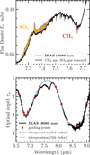 |
Fig. 3 Removal of gas phase lines and local continuum estimate. Top: contribution of gas phase SO2 emission (yellow) and CH4 absorption (red) lines estimated from the observed IRAS 18089 mm spectrum (gray). The corrected spectrum is shown in black. Bottom: corrected optical depth spectrum (black) and the local continuum interpolation (blue line). The red dots mark the guiding points used for the interpolation. The green dashed line shows the continuum interpolation based on a fifth-order polynomial (see Appendix E). |
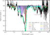 |
Fig. 4 Optical depth spectrum of IRAS 18089 mm after local continuum subtraction. The observed optical depth spectrum is presented in black, highlighting the absorption features by minor ice constituents. The total fit considering a mixture of ice species is shown by the thick dashed green line. The solid lines are contributions by each ice species (details on the laboratory data are summarized in Table C.1). |
3.2 Gas phase abundances using mm spectra
Gas phase molecules can be easily observed through their rotational levels at (sub)mm wavelengths. The observed 3 mm spectra obtained with ALMA are presented in Figs. D.1 and D.2. Many spectral lines are detected covering simple molecular species with strong line emission, but there is a forest of weak COM lines in addition.
Figure D.3 shows line-integrated intensity maps of SiO, SO2, HC13CCN, 13CH3OH, C2H5OH, and CH3OCH3 transitions. While SiO is tracing the outflow launched by the mm source (consistent with low resolution SiO (5 - 4) data, Beuther et al. 2004), the spatially resolved emission of COMs, including less abundant isotopologs, as well as S- and N-bearing species, are tracing the hot core region of IRAS 18089 mm. In contrast, there is no significant molecular gas phase emission at the location of the nearby MIR source.
The molecular column densities of the gas phase species can be inferred using the XCLASS tool (Möller et al. 2017). With XCLASS, the radiative transfer equation of each identified molecule is solved assuming LTE. The optical depth τν of each transition is taken into account in the calculation of the synthetic model spectra (i.e., we do not assume that the transitions are all optically thin). The best-fit evaluated based on a least χ2 analysis. The fit parameters are the source size, θsource, rotation temperature, Trot, column density, N, full width at half maximum (FWHM) line width, ∆v, and velocity offset, voff. We fixed the source size to the aperture size of the extracted spectra (diameter of 2″); hence, we assumed the emission was spatially resolved (which is the case even for transitions of less abundant isotopologs, Fig. D.3) and the beam filling factor is ∼1.
For the χ2 minimization procedure of the remaining four parameters, we used an algorithm chain of the Genetic and Levenberg-Marquart algorithms, using 50 iterations each per molecule. Uncertainties of the fit parameters are estimated using the MCMC algorithm (Foreman-Mackey et al. 2013). We fit a total of 38 different species, also considering different isotopologs and torsionally or vibrationally excited states, all summarized in Table D.1. The ALMA 3 mm spectra trace various types of molecules, including O-, N-, and S-bearing species as well as SiO. Table D.1 also shows which catalog was used for each species for the XCLASS fitting. For each species, all spectral windows are included in the XCLASS fitting approach. Due to the line rich spectra, some transitions (in particular, weaker COM lines) end up blended at our spectral resolution of 0.9 and 3.4km s−1 (Figs. D.1 and D.2). However since the dataset covers a large bandwidth, the presence of many detected COM transitions ensures that line blending does not impact the XCLASS fit.
The results for the gas column density of all species is listed in Table D.1 and the total best-fit spectrum is presented in Figs. D.1 and D.2. In Sect. 4.1, we compare and discuss the abundances of molecules in the gas phase and in the ices.
4 Discussion
In this work, we analyzed both the molecular ice and gas phase column densities toward the hot core region (∼5000 au) in IRAS 18089. Sensitive JWST and ALMA observations reveal a rich ice chemical composition in the solid state and gas phase. In Sect. 4.1, we discuss the ice and gas phase abundances toward the IRAS 18089 hot core in comparison with low-mass hot core sources (Chen et al. 2024) and a hot core model (Garrod et al. 2022). In Sect. 4.2, we further compare the ice composition of IRAS 18089 with low- and high-mass star-forming regions targeted by recent JWST observations.
4.1 Ice and gas phase abundances in the IRAS 18089 hot core
A comparison of relative ice and gas phase abundances toward IRAS 18089 is presented in Fig. 5 using JWST/MIRI-MRS and ALMA 3 mm observations (Table D.1). Given that gas phase H2O transitions were not covered in the ALMA 3 mm setup and the CH3OH ice column density could not be directly inferred from the JWST/MIRI-MRS data, we show molecular abundances relative to C2H5OH for which column density estimates are available for both gas and ice phases. Thus, in the following, our comparison is always based on abundances relative to C2H5OH, unless stated otherwise. For completeness, we show molecular abundances relative to CH3OH (with the ice column density only indirectly inferred from the nearby MIR position, Sect. 3.1) in Fig. D.4. With both C2H5OH and CH3OH as reference species the same trends can be observed.
In Fig. 5 (as well as Fig. D.4 and Table D.1) the column density of less abundant isotopologs covered by ALMA were converted to their main isotopolog using 12 C/13 C=50, 16O/18O=372, 32S∕34S=22 (Wilson & Rood 1994) and 32S/33S=86 (Yan et al. 2023) with a Galactocentric distance of dgal=5.7kpc for IRAS 18089. The results in Fig. 5 are grouped by C/O-, N-, S-, and Si-bearing species.
In general, most O-bearing molecules have the highest relative abundance, followed by S-bearing, and then N-bearing molecules and with SiO having the lowest relative abundance. While CH3OCHO is abundant in the gas phase, we did not find significant contributions in the ice spectrum (Fig. 4). For HCOOH and CH3COOH we carefully checked the ALMA spectra for line detections, finding that the non-detection in the gas phase might be either linked to strong transitions not covered in the ALMA 3 mm setup or the fact that these species are not abundant in the gas phase. Assuming Trot = 100 K and ∆v = 5 km s−1 (mean values from all detected species), we estimated upper limits of 5 × 1016 cm−2 and 1 × 1016 cm−2 for the HCOOH and CH3 COOH gas phase column densities which is less than the derived ice column densities (Table D.1).
We find a good agreement between CH3 OH ice and gas phase abundance, even though the CH3 OH ice column density could be only indirectly inferred from the IRAS 18089 MIR source. This is consistent with the ice composition of IRAS 18089 mm and MIR sources being similar in general (w.r.t. H2O ice, Fig. 7), as further discussed in Sect. 4.2. Within the uncertainties we find a good agreement between CH3OCH3 ice and gas phase abundances. Relative to CH3OH, the C2H5OH abundance in the ice and gas phase also agree with each other (Fig. D.4). However, not all species show the same abundances in the gas and ice phase. For CH3CHO, the abundance is more than one order of magnitude higher in the ice compared to the gas phase and for SO2 and CH3COCH3 the gas phase abundance is about one order of magnitude higher, compared to the ice abundance.
We find a high abundance of OCN− ice, similar to HCN in the gas phase. Recently, there has been a tentative detection of CH3CN ice (Nazari et al. 2024). We checked the IRAS 18089 ice spectrum (Fig. 4), but similar to other low- and high-mass protostars (Chen et al. 2024; van Dishoeck et al. 2025; Sewiło et al. 2025), there is no detection of CH3CN in the ice using MIRI-MRS data. A more detailed investigation of N-bearing ices requires additional NIRSpec observations (Nazari et al. 2024).
Many S-bearing isotopologs (from CS, SO, SO2, OCS, and H2CS) are very abundant in the gas phase. Our results for the SO2 ice and gas phase abundance relative to CH3OH (0.02 and 0.1, respectively) are in agreement with a recent study by Santos et al. (2024b, their Fig. 6). These authors compared the gas phase SO2 abundance (relative to CH3OH) obtained in a sample of HMSFRs with ALMA with ice abundances from Boogert et al. (1997) and obtain ≈0.1 for both phases. Only one detection and one upper limit could be inferred for SO2 ice toward HMSFRs in the study by Boogert et al. (1997) highlighting the need for more measurements in the future. There is a hint at OCS ice absorption at 4.9 μm in the MIRI-MRS spectrum (Fig. 2), however it is at the edge of the covered wavelength range. OCS ice has been detected toward many HMSFRs (Boogert et al. 2022). Additional JWST/NIRSpec data is essential to better constrain the sulfur inventory of the ices. Since the simpler S-bearing molecule ice features are covered by NIRSpec, for which IRAS 18089 has no available data, and only a few laboratory works were dedicated to S-bearing COMs (Santos et al. 2024a; Narayanan et al. 2025), future effort toward S-bearing species is necessary.
Chen et al. (2024) has conducted a direct comparison between ice and gas phase abundances of COMs toward the two low-mass protostars IRAS 2A and B1-c (which are both low-mass hot core sources located in the Perseus molecular cloud, e.g., Bottinelli et al. 2007; van Gelder et al. 2022; Busch et al. 2025). The ice composition of IRAS 2A was previously analyzed by Rocha et al. (2024). In Fig. 6 we show ice and gas phase abundances of COMs (relative to CH3OH) detected toward IRAS 18089 mm and include the results obtained for the low-mass hot cores studied by Chen et al. (2024) (excluding data for which only upper limits could be constrained).
A comprehensive gas-grain chemical model of a hot core has already been carried out by Garrod et al. (2022). One of their model setups included a fast warm-up stage, which is most suitable for high-mass hot cores that evolve on fast evolutionary timescales. For comparison we show in Fig. 6 the ice and gas phase abundances relative to CH3OH for this model setup at T = 100 K (their Fig. 10).
Figure 6 reveals that the low- and high-mass hot cores have comparable (within one order of magnitude) ice abundances (relative to CH3OH) for all presented species. This highlights that for COM formation the early cold stage is essential. The gas phase abundances of CH3OCHO and C2H5OH are enhanced in the case of the high-mass hot core. The ice abundances of the hot core model agree with the observed hot cores for CH3OCHO, C2H5OH, and CH3OCH3. The ice abundances of CH3CHO and CH3 COOH are under-predicted in the hot core model by more than one order of magnitude.
In the case of CH3CHO, the hot core model predicts in addition a higher gas phase abundance compared to what is observed for the hot cores. Despite taking into account more reaction pathways for the formation of CH3CHO in the hot core model (Sect. 5.3 in Garrod et al. 2022), whereas only CH3 + HCO was considered the dominant reaction in diffusion-only models, there is a systematic difference between observations and models.
We find that for the IRAS 18089 hot core region, some species have similar abundances in the ice and gas phase (CH3OH, C2H5OH, CH3OCH3). On the other hand, SO2 and CH3COCH3 have higher abundances in the gas phase, suggesting the importance of additional gas phase routes. Most notably, in the case of CH3CHO, we find a disagreement of the predicted ice and gas phase column density by the models from Garrod et al. (2022) in contrast to the observed values toward low-mass (Chen et al. 2024) and high-mass hot cores (this work). The hot core model by Garrod et al. (2022) predicts that the CH3CHO ice abundance should be one order of magnitude lower compared to its gas phase abundance. However, the observations toward both low-mass and high-mass hot cores reveal an opposite trend with the CH3CHO ice abundance that is between one and two orders of magnitudes higher than what is measured in the gas phase. Future work requires a statistical analysis of ice and gas abundances of low- and high-mass protostars as well as applying physical-chemical modeling of specific sources to better understand the chemical links between different molecules (Simons et al. 2020; Gieser et al. 2021; Garrod et al. 2022).
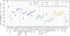 |
Fig. 5 Comparison of ice and gas phase abundances (relative to C2H5OH) toward IRAS 18089 mm. The crosses and squares mark ice and gas phase abundances, respectively. Blue, green, yellow, and red colors highlight COH-, N-, S-, and Si-bearing species. The column density of less abundant isotopologs (including 13C, 18O, 33S, and 34 S isotopes) were converted to their main isotopolog using relations by Wilson & Rood (1994) and Yan et al. (2023) with a Galactocentric distance of dgal=5.7kpc for IRAS 18089. |
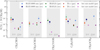 |
Fig. 6 Comparison of ice and gas phase abundances (relative to CH3OH) toward low- and high-mass hot cores. The crosses and squares mark ice and gas phase abundances, respectively. Blue, green, and red data points are IRAS 18089 mm (this work), IRAS 2A (Chen et al. 2024; Rocha et al. 2024), and B1-c (Chen et al. 2024). The pink data points are taken from the hot core model by Garrod et al. (2022) (the fast warm-up model at T=100 K; see their Fig. 10). |
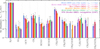 |
Fig. 7 Comparison of ice abundances (relative to H2O) toward low- and highmass protostars. The abundances toward the IRAS 18089 mm analyzed in this work is shown in blue. The results for the low-mass protostars B1-c (red) and IRAS 2A (orange) were taken from Chen et al. (2024). The high-mass protostar IRAS 23385 (green) and MIR peak of IRAS 18089 (pink) were analyzed in Rocha et al. (2024) and van Dishoeck et al. (2025), respectively. The ST6 source located in the LMC was studied by Sewiło et al. (2025) and is shown in purple. Upper limits are indicated by gray bars and triangle data points. |
4.2 Ice composition in low- and high-mass protostars
Spectroscopic observations with JWST allow for a detailed characterization of minor ice constituents. Due to the overlap of ice bands of many different molecular species in the 6.5 to 9.0 μm range (Fig. 4) the extraction of individual components is non trivial, and thus the ice composition in this range has so far only been analyzed in a limited sample of protostars observed with JWST. The composition can be determined by using a linear combination of different molecular ices (Chen et al. 2024, and this work) or using tools such as ENIIGMA (Rocha et al. 2021, 2024) and INDRA (Rayalacheruvu et al. 2025). In this section we focus on a comparison between ice abundances (relative to H2O ice) of the protostars for which their ice composition has been analyzed so far. We note that even though different methods were used to estimate ice column densities, overall these different techniques provide similar results.
A comparison of ice abundances (relative to H2O ice) for in total five protostars with the chemical inventory of the ices of the IRAS 18089 mm hot core is presented in Fig. 7. The ices toward the low-mass protostars B1-c and IRAS 2A were studied in Chen et al. (2024) and Rocha et al. (2024) and toward the high-mass protostars IRAS 23385 and the MIR source of IRAS 18089 in Rocha et al. (2024) and van Dishoeck et al. (2025), respectively. We also compare our results with the ice composition of the ST6 protostar located in the Large Magellanic Cloud (LMC) which is a lower metallicity environment compared to the Milky Way (Sewiło et al. 2025). The Galactic sources in Fig. 7 are sorted by Galactocentric distance.
In general, SO2 has a similar relative ice abundance of ≈ 10−3. For OCN− ice we find a slightly lower ice abundances toward low metallicity environments, but note that in previous work a second ice band was not considered (Sect. 3.1). For HCOO− we find an ice abundance about one order of magnitude higher compared to other protostars. We note that the location of the two HCOO−ice bands (7.2 and 7.4 μm) are sensitive to the local continuum estimate (Fig. 3). However, the high abundance can be explained by thermal processing due to protostellar heating. In laboratory experiments, the amount of HCOO− ions is increased after heating ice mixtures containing NH3 and HCOOH (Sect. 4 in Gálvez et al. 2010).
For most of the analyzed ice species, the ice abundances are within the uncertainties similar across the different Galactic protostars, namely SO2, CH4, HCOOH, CH3OH, CH3CHO, CH3COOH, C2H5OH, and CH3COCH3. For CH3OCH3 the ice abundance of both IRAS 18089 mm and MIR are about one order of magnitude higher compared to the low-mass hot core B1-c. For the extragalactic ST6 source the ice abundances are systematically lower. This can be linked to the lower metallicity in the LMC compared to the Milky Way. In addition, there are hints at trends with Galactocentric radius for OCN−, CH3OH, and CH3CHO. Due to a decreasing metallicity with increasing Galactocentric distance, the destruction of molecules is more efficient.
In summary, within the uncertainties we do not find large variations of ice abundances among different Galactic sources. This stresses the importance of grain-surface chemistry in the cold stages of the star formation phase. Comparing the ices with the ST6 source in the LMC highlights the impact of metallicity on the molecular composition. Further studies at different Galactic radii are essential to investigate this trend within the Milky Way. However, since the number of analyzed sources (in both their gas phase and ice composition) is still low, two low-mass protostars (Chen et al. 2024; Rocha et al. 2024) and one highmass protostar (this work), to investigate general trends requires a larger sample. However, our results underline the importance of sensitive spectroscopic observations with JWST (including the recently approved programs with IDs 5804 and 8887) to better understand the formation of molecules in the interstellar medium.
5 Conclusions
In this work, we analyze the molecular composition in the ice and gas phase toward the hot core IRAS 18089 mm using sensitive and high resolution observations with JWST/MIRI-MRS and ALMA. Our main findings are summarized in the following.
The JWST/MIRI-MRS spectrum from 5 to 28 μm shows emission and absorption lines by gas phase species as well as absorption features by silicates and ices. The continuum SED is well characterized by two embedded (hot at T=410 K and warm at T=80 K) modified black bodies, absorbed by carbonaceous and silicate dust and water ice. The total H2O water ice column density is 1.5×1019 cm−2. Due to the strong silicate absorption at 10 μm reaching the noise floor (a behavior that is expected for other bright high-mass protostars as well), the H2O water ice column density can only be constrained within an uncertainty of 50% and also stands in the way of a direct estimate of the CH3OH ice column density.
The optical depth spectrum toward the COM region (from 6.5 to 9.0 μm) consists of a variety of different ice species including SO2, OCN−, CH4, HCOO−, HCOOH, CH3CHO, CH3COOH, C2H5OH, CH3OCH3, and CH3OCH3. The column density of these ices are in the range of ∼1016-1017 cm−2.
The ALMA data at 3 mm reveal line-rich spectra originating from a variety of different gas phase molecules from simple diatomic species to COMs, including O-, N-, S-bearing species as well as less abundant isotopologs and torsionally or vibrationally excited transitions. On average, we find that gas phase abundances of O-bearing COMs are about one to two orders of magnitude higher compared to S-bearing and N-bearing species, respectively.
Comparing the IRAS 18089 mm ice and gas phase abundances (relative to C2H5OH or CH3OH), we find similar abundances in both phases for C2H5OH, CH3OH, and CH3OCH3. The abundances of SO2 and CH3COCH3 are elevated in the gas phase, suggesting additional gas phase formation routes. The ice abundance of CH3CHO is one order of magnitude higher in the ices compared to the gas phase. This is in contrast to what is predicted from the hot core chemical model described by Garrod et al. (2022). Overall, we find the same trends for this high-mass hot core studied in this work and two low-mass hot cores analyzed by Chen et al. (2024).
The ice abundances (relative to H2O ice) toward IRAS 18089 mm are comparable to other Galactic low- and high-mass protostars. In particular, the ice abundances are similar to the nearby IRAS 18089 MIR position providing a nearby background source to probe the ice composition offset from the hot core region. There are hints of a decreasing abundance with Galactocentric distance for OCN−, CH3OH, and CH3CHO.
JWST/MIRI-MRS observations have revealed a complex composition of molecular ices toward a number of low- and highmass star-forming regions. To better understand the variations of the ice and gas compositions between regions, a larger sample across different environments and evolutionary stages must be probed. To better characterize N-bearing and S-bearing ices, access to additional NIRSpec data of high-mass protostars is essential.
Acknowledgements
This work is based on observations made with the NASA/ESA/CSA James Webb Space Telescope. The data were obtained from the Mikulski Archive for Space Telescopes at the Space Telescope Science Institute, which is operated by the Association of Universities for Research in Astronomy, Inc., under NASA contract NAS 5-03127 for JWST. These observations are associated with program #1290. The following National and International Funding Agencies funded and supported the MIRI development: NASA; ESA; Belgian Science Policy Office (BELSPO); Centre Nationale d’Etudes Spatiales (CNES); Danish National Space Centre; Deutsches Zentrum fur Luft und Raumfahrt (DLR); Enterprise Ireland; Ministerio De Economiá y Competividad; Netherlands Research School for Astronomy (NOVA); Netherlands Organisation for Scientific Research (NWO); Science and Technology Facilities Council; Swiss Space Office; Swedish National Space Agency; and UK Space Agency. This paper makes use of the following ALMA data: ADS/JAO.ALMA#2018.1.00424.S ALMA is a partnership of ESO (representing its member states), NSF (USA) and NINS (Japan), together with NRC (Canada), NSTC and ASIAA (Taiwan), and KASI (Republic of Korea), in cooperation with the Republic of Chile. The Joint ALMA Observatory is operated by ESO, AUI/NRAO and NAOJ. A.C.G. acknowledges support from PRIN-MUR 2022 20228JPA3A “The path to star and planet formation in the JWST era (PATH)” funded by NextGeneration EU and by INAF-GoG 2022 “NIR-dark Accretion Outbursts in Massive Young stellar objects (NAOMY)” and Large Gran INAF-2024 “Spectral Key fea-tures of Young stellar objects: Wind-Accretion LinKs Explored in the infraRed (SKYWALKER)”. J.M.V. acknowledges support from the Academy of Finland grant No 348342. Astrochemistry in Leiden is supported by funding from the European Research Council (ERC) under the European Union’s Horizon 2020 research and innovation program (grant agreement No. 291141 MOLDISK), and by NOVA and NWO through TOP-1 grant 614.001.751 and its Dutch Astrochemistry Program (DANII). The present work is closely connected to ongoing research within InterCat, the Center for Interstellar Catalysis located in Aarhus, Denmark.
References
- Argyriou, I., Glasse, A., Law, D. R., et al. 2023, A&A, 675, A111 [NASA ADS] [CrossRef] [EDP Sciences] [Google Scholar]
- Beltrán, M. T., & de Wit, W. J. 2016, A&A Rev., 24, 6 [CrossRef] [Google Scholar]
- Beuther, H., Schilke, P., Menten, K. M., et al. 2002a, ApJ, 566, 945 [NASA ADS] [CrossRef] [Google Scholar]
- Beuther, H., Schilke, P., Sridharan, T. K., et al. 2002b, A&A, 383, 892 [NASA ADS] [CrossRef] [EDP Sciences] [Google Scholar]
- Beuther, H., Hunter, T. R., Zhang, Q., et al. 2004, ApJ, 616, L23 [NASA ADS] [CrossRef] [Google Scholar]
- Beuther, H., Churchwell, E. B., McKee, C. F., & Tan, J. C. 2007, in Protostars and Planets V, eds. B. Reipurth, D. Jewitt, & K. Keil (Tucson: University of Arizona Press), 165 [Google Scholar]
- Beuther, H., Mottram, J. C., Ahmadi, A., et al. 2018, A&A, 617, A100 [NASA ADS] [CrossRef] [EDP Sciences] [Google Scholar]
- Beuther, H., van Dishoeck, E. F., Tychoniec, L., et al. 2023, A&A, 673, A121 [NASA ADS] [CrossRef] [EDP Sciences] [Google Scholar]
- Bisschop, S. E., Fuchs, G. W., Boogert, A. C. A., van Dishoeck, E. F., & Linnartz, H. 2007, A&A, 470, 749 [NASA ADS] [CrossRef] [EDP Sciences] [Google Scholar]
- Boogert, A. C. A., Schutte, W. A., Helmich, F. P., Tielens, A. G. G. M., & Wooden, D. H. 1997, A&A, 317, 929 [NASA ADS] [Google Scholar]
- Boogert, A. C. A., Gerakines, P. A., & Whittet, D. C. B. 2015, ARA&A, 53, 541 [Google Scholar]
- Boogert, A. C. A., Brewer, K., Brittain, A., & Emerson, K. S. 2022, ApJ, 941, 32 [NASA ADS] [CrossRef] [Google Scholar]
- Bottinelli, S., Ceccarelli, C., Williams, J. P., & Lefloch, B. 2007, A&A, 463, 601 [NASA ADS] [CrossRef] [EDP Sciences] [Google Scholar]
- Bouscasse, L., Csengeri, T., Wyrowski, F., Menten, K. M., & Bontemps, S. 2024, A&A, 686, A252 [NASA ADS] [CrossRef] [EDP Sciences] [Google Scholar]
- Brunken, N. G. C., van Dishoeck, E. F., Slavicinska, K., et al. 2024, A&A, 692, A163 [NASA ADS] [CrossRef] [EDP Sciences] [Google Scholar]
- Busch, L. A., Pineda, J. E., Sipilä, O., et al. 2025, A&A, 699, A359 [NASA ADS] [CrossRef] [EDP Sciences] [Google Scholar]
- Bushouse, H., Eisenhamer, J., Dencheva, N., et al. 2024, https://doi.org/10.5281/zenodo.10463537 [Google Scholar]
- Cesaroni, R., Felli, M., Testi, L., Walmsley, C. M., & Olmi, L. 1997, A&A, 325, 725 [NASA ADS] [Google Scholar]
- Chen, Y., van Gelder, M. L., Nazari, P., et al. 2023, A&A, 678, A137 [NASA ADS] [CrossRef] [EDP Sciences] [Google Scholar]
- Chen, Y., Rocha, W. R. M., van Dishoeck, E. F., et al. 2024, A&A, 690, A205 [NASA ADS] [CrossRef] [EDP Sciences] [Google Scholar]
- Churchwell, E. 2002, ARA&A, 40, 27 [Google Scholar]
- Coletta, A., Fontani, F., Rivilla, V. M., et al. 2020, A&A, 641, A54 [NASA ADS] [CrossRef] [EDP Sciences] [Google Scholar]
- Dale, J. E., Ercolano, B., & Bonnell, I. A. 2012, MNRAS, 424, 377 [NASA ADS] [CrossRef] [Google Scholar]
- Dartois, E., Schutte, W., Geballe, T. R., et al. 1999, A&A, 342, L32 [NASA ADS] [Google Scholar]
- De Buizer, J. M., Liu, M., Tan, J. C., et al. 2017, ApJ, 843, 33 [Google Scholar]
- de Wit, W. J., Hoare, M. G., Oudmaijer, R. D., & Lumsden, S. L. 2010, A&A, 515, A45 [NASA ADS] [CrossRef] [EDP Sciences] [Google Scholar]
- Dominik, C., Min, M., & Tazaki, R. 2021, Astrophysics Source Code Library [record ascl:2104.010] [Google Scholar]
- Ehrenfreund, P., Dartois, E., Demyk, K., & D’Hendecourt, L. 1998, A&A, 339, L17 [NASA ADS] [Google Scholar]
- Foreman-Mackey, D., Hogg, D. W., Lang, D., & Goodman, J. 2013, PASP, 125, 306 [Google Scholar]
- Francis, L., van Gelder, M. L., van Dishoeck, E. F., et al. 2024, A&A, 683, A249 [NASA ADS] [CrossRef] [EDP Sciences] [Google Scholar]
- Gálvez, O., Maté, B., Herrero, V. J., & Escribano, R. 2010, ApJ, 724, 539 [NASA ADS] [CrossRef] [Google Scholar]
- Gardner, J. P., Mather, J. C., Abbott, R., et al. 2023, PASP, 135, 068001 [NASA ADS] [CrossRef] [Google Scholar]
- Garrod, R. T., & Herbst, E. 2006, A&A, 457, 927 [NASA ADS] [CrossRef] [EDP Sciences] [Google Scholar]
- Garrod, R. T., Jin, M., Matis, K. A., et al. 2022, ApJS, 259, 1 [NASA ADS] [CrossRef] [Google Scholar]
- Gerakines, P. A., Materese, C. K., & Hudson, R. L. 2025, MNRAS, 537, 2918 [Google Scholar]
- Gerner, T., Beuther, H., Semenov, D., et al. 2014, A&A, 563, A97 [NASA ADS] [CrossRef] [EDP Sciences] [Google Scholar]
- Gibb, E. L., Whittet, D. C. B., Boogert, A. C. A., & Tielens, A. G. G. M. 2004, ApJS, 151, 35 [NASA ADS] [CrossRef] [Google Scholar]
- Gibb, E. L., Whittet, D. C. B., Schutte, W. A., et al. 2000, ApJ, 536, 347 [Google Scholar]
- Gieser, C., Beuther, H., Semenov, D., et al. 2021, A&A, 648, A66 [EDP Sciences] [Google Scholar]
- Gieser, C., Beuther, H., Semenov, D., et al. 2023a, A&A, 674, A160 [NASA ADS] [CrossRef] [EDP Sciences] [Google Scholar]
- Gieser, C., Beuther, H., van Dishoeck, E. F., et al. 2023b, A&A, 679, A108 [NASA ADS] [CrossRef] [EDP Sciences] [Google Scholar]
- Gigli, D., Fontani, F., Colzi, L., et al. 2025, A&A, 704, A171 [NASA ADS] [CrossRef] [EDP Sciences] [Google Scholar]
- Ginsburg, A., McGuire, B. A., Sanhueza, P., et al. 2023, ApJ, 942, 66 [Google Scholar]
- Goedhart, S., Langa, M. C., Gaylard, M. J., & Van Der Walt, D. J. 2009, MNRAS, 398, 995 [NASA ADS] [CrossRef] [Google Scholar]
- Gommers, R., Virtanen, P., Haberland, M., et al. 2024, scipy/scipy: SciPy 1.13.1 [Google Scholar]
- Gross, R. E., Yang, Y.-L., Cleeves, L. I., et al. 2026, ApJ, 998, 68 [Google Scholar]
- Herbst, E., & van Dishoeck, E. F. 2009, ARA&A, 47, 427 [NASA ADS] [CrossRef] [Google Scholar]
- Jones, O. C., Álvarez-Márquez, J., Sloan, G. C., et al. 2023, MNRAS, 523, 2519 [Google Scholar]
- Klaassen, P. D., Johnston, K. G., Urquhart, J. S., et al. 2018, A&A, 611, A99 [NASA ADS] [CrossRef] [EDP Sciences] [Google Scholar]
- Kumar, M. S. N., Palmeirim, P., Arzoumanian, D., & Inutsuka, S. I. 2020, A&A, 642, A87 [EDP Sciences] [Google Scholar]
- Law, D. D., Morrison, J. E., Argyriou, I., et al. 2023, AJ, 166, 45 [NASA ADS] [CrossRef] [Google Scholar]
- Louvet, F., Sanhueza, P., Stutz, A., et al. 2024, A&A, 690, A33 [NASA ADS] [CrossRef] [EDP Sciences] [Google Scholar]
- Lu, X., Zhang, Q., Liu, H. B., et al. 2018, ApJ, 855, 9 [Google Scholar]
- Mastrapa, R. M., Sandford, S. A., Roush, T. L., Cruikshank, D. P., & Dalle Ore, C. M. 2009, ApJ, 701, 1347 [NASA ADS] [CrossRef] [Google Scholar]
- McClure, M. K., Rocha, W. R. M., Pontoppidan, K. M., et al. 2023, Nat. Astron., 7, 431 [NASA ADS] [CrossRef] [Google Scholar]
- Möller, T., Endres, C., & Schilke, P. 2017, A&A, 598, A7 [NASA ADS] [CrossRef] [EDP Sciences] [Google Scholar]
- Motte, F., Bontemps, S., & Louvet, F. 2018, ARA&A, 56, 41 [NASA ADS] [CrossRef] [Google Scholar]
- Müller, H. S. P., Schlöder, F., Stutzki, J., & Winnewisser, G. 2005, J. Mol. Struc., 742, 215 [Google Scholar]
- Nakibov, R., Karteyeva, V., Petrashkevich, I., et al. 2025, ApJ, 978, L46 [Google Scholar]
- Narayanan, S., Piacentino, E. L., Öberg, K. I., & Rajappan, M. 2025, ApJ, 986, 10 [Google Scholar]
- Nazari, P. 2026, Life Sci. Space Res., 49, 4 [Google Scholar]
- Nazari, P., Rocha, W. R. M., Rubinstein, A. E., et al. 2024, A&A, 686, A71 [NASA ADS] [CrossRef] [EDP Sciences] [Google Scholar]
- Nightingale, R. E., & Wagner, E. L. 1954, J. Chem. Phys., 22, 203 [Google Scholar]
- Novozamsky, J. H., Schutte, W. A., & Keane, J. V. 2001, A&A, 379, 588 [NASA ADS] [CrossRef] [EDP Sciences] [Google Scholar]
- Öberg, K. I., Fraser, H. J., Boogert, A. C. A., et al. 2007, A&A, 462, 1187 [NASA ADS] [CrossRef] [EDP Sciences] [Google Scholar]
- Öberg, K. I., Garrod, R. T., van Dishoeck, E. F., & Linnartz, H. 2009, A&A, 504, 891 [NASA ADS] [CrossRef] [EDP Sciences] [Google Scholar]
- Perotti, G., Jørgensen, J. K., Fraser, H. J., et al. 2021, A&A, 650, A168 [NASA ADS] [CrossRef] [EDP Sciences] [Google Scholar]
- Pickett, H. M., Poynter, R. L., Cohen, E. A., et al. 1998, J. Quant. Spec. Radiat. Transf., 60, 883 [Google Scholar]
- Pollack, J. B., Hollenbach, D., Beckwith, S., et al. 1994, ApJ, 421, 615 [Google Scholar]
- Rachid, M. G., Terwisscha van Scheltinga, J., Koletzki, D., & Linnartz, H. 2020, A&A, 639, A4 [EDP Sciences] [Google Scholar]
- Ramírez-Tannus, M. C., Bik, A., Getman, K. V., et al. 2025, A&A, 701, A139 [NASA ADS] [CrossRef] [EDP Sciences] [Google Scholar]
- Rathborne, J. M., Jackson, J. M., & Simon, R. 2006, ApJ, 641, 389 [Google Scholar]
- Raunier, S., Chiavassa, T., Marinelli, F., Allouche, A., & Aycard, J.-P. 2003, J. Phys. Chem. A, 107, 9335 [Google Scholar]
- Rayalacheruvu, P., Majumdar, L., Rocha, W. R. M., et al. 2025, ApJS, 281, 51 [Google Scholar]
- Reyes-Reyes, S. D., Beuther, H., van Dishoeck, E. F., et al. 2026, A&A, 709, A13 [NASA ADS] [CrossRef] [EDP Sciences] [Google Scholar]
- Rieke, G. H., Wright, G. S., Böker, T., et al. 2015, PASP, 127, 584 [NASA ADS] [CrossRef] [Google Scholar]
- Rigby, J., Perrin, M., McElwain, M., et al. 2023, PASP, 135, 048001 [NASA ADS] [CrossRef] [Google Scholar]
- Rocha, W. R. M., Pilling, S., de Barros, A. L. F., et al. 2017, MNRAS, 464, 754 [NASA ADS] [CrossRef] [Google Scholar]
- Rocha, W. R. M., Perotti, G., Kristensen, L. E., & Jørgensen, J. K. 2021, A&A, 654, A158 [NASA ADS] [CrossRef] [EDP Sciences] [Google Scholar]
- Rocha, W. R. M., Rachid, M. G., Olsthoorn, B., et al. 2022, A&A, 668, A63 [NASA ADS] [CrossRef] [EDP Sciences] [Google Scholar]
- Rocha, W. R. M., van Dishoeck, E. F., Ressler, M. E., et al. 2024, A&A, 683, A124 [NASA ADS] [CrossRef] [EDP Sciences] [Google Scholar]
- Rocha, W. R. M., McClure, M. K., Sturm, J. A., et al. 2025, A&A, 693, A288 [NASA ADS] [CrossRef] [EDP Sciences] [Google Scholar]
- Sabatini, G., Bovino, S., Giannetti, A., et al. 2021, A&A, 652, A71 [NASA ADS] [CrossRef] [EDP Sciences] [Google Scholar]
- Salyk, C., Pontoppidan, K. M., Blake, G. A., Najita, J. R., & Carr, J. S. 2011, ApJ, 731, 130 [Google Scholar]
- Sanhueza, P., Contreras, Y., Wu, B., et al. 2019, ApJ, 886, 102 [Google Scholar]
- Sanhueza, P., Girart, J. M., Padovani, M., et al. 2021, ApJ, 915, L10 [NASA ADS] [CrossRef] [Google Scholar]
- Santos, J. C., Enrique-Romero, J., Lamberts, T., Linnartz, H., & Chuang, K.-J. 2024a, ACS Earth Space Chem., 8, 1646 [Google Scholar]
- Santos, J. C., van Gelder, M. L., Nazari, P., Ahmadi, A., & van Dishoeck, E. F. 2024b, A&A, 689, A248 [NASA ADS] [CrossRef] [EDP Sciences] [Google Scholar]
- Schutte, W. A., Boogert, A. C. A., Tielens, A. G. G. M., et al. 1999, A&A, 343, 966 [NASA ADS] [Google Scholar]
- Sewiło, M., Rocha, W. R. M., van Gelder, M., et al. 2025, ApJ, 992, L30 [Google Scholar]
- Shirley, Y. L., Evans, II, N. J., Young, K. E., Knez, C., & Jaffe, D. T. 2003, ApJS, 149, 375 [NASA ADS] [CrossRef] [Google Scholar]
- Simons, M. A. J., Lamberts, T., & Cuppen, H. M. 2020, A&A, 634, A52 [NASA ADS] [CrossRef] [EDP Sciences] [Google Scholar]
- Slavicinska, K., van Dishoeck, E. F., Tychoniec, L., et al. 2024, A&A, 688, A29 [NASA ADS] [CrossRef] [EDP Sciences] [Google Scholar]
- Slavicinska, K., Tychoniec, L., Navarro, M. G., et al. 2025, ApJ, 986, L19 [Google Scholar]
- Smith, Z. L., Dickinson, H. J., Fraser, H. J., et al. 2025, Nat. Astron., 9, 883 [Google Scholar]
- Sridharan, T. K., Beuther, H., Schilke, P., Menten, K. M., & Wyrowski, F. 2002, ApJ, 566, 931 [Google Scholar]
- Terwisscha van Scheltinga, J., Ligterink, N. F. W., Boogert, A. C. A., van Dishoeck, E. F., & Linnartz, H. 2018, A&A, 611, A35 [NASA ADS] [CrossRef] [EDP Sciences] [Google Scholar]
- Terwisscha van Scheltinga, J., Marcandalli, G., McClure, M. K., Hogerheijde, M. R., & Linnartz, H. 2021, A&A, 651, A95 [NASA ADS] [CrossRef] [EDP Sciences] [Google Scholar]
- Tyagi, H., Manoj, P., Narang, M., et al. 2025, ApJ, 983, 110 [Google Scholar]
- Urquhart, J. S., König, C., Giannetti, A., et al. 2018, MNRAS, 473, 1059 [Google Scholar]
- van Broekhuizen, F. A., Pontoppidan, K. M., Fraser, H. J., & van Dishoeck, E. F. 2005, A&A, 441, 249 [NASA ADS] [CrossRef] [EDP Sciences] [Google Scholar]
- van der Tak, F. F. S., van Dishoeck, E. F., Evans, II, N. J., & Blake, G. A. 2000, ApJ, 537, 283 [NASA ADS] [CrossRef] [Google Scholar]
- van Dishoeck, E. F., Tychoniec, L., Rocha, W. R. M., et al. 2025, A&A, 699, A361 [NASA ADS] [CrossRef] [EDP Sciences] [Google Scholar]
- van Gelder, M. L., Nazari, P., Tabone, B., et al. 2022, A&A, 662, A67 [NASA ADS] [CrossRef] [EDP Sciences] [Google Scholar]
- van Gelder, M. L., Francis, L., van Dishoeck, E. F., et al. 2024a, A&A, 692, A197 [NASA ADS] [CrossRef] [EDP Sciences] [Google Scholar]
- van Gelder, M. L., Ressler, M. E., van Dishoeck, E. F., et al. 2024b, A&A, 682, A78 [NASA ADS] [CrossRef] [EDP Sciences] [Google Scholar]
- Whittet, D. C. B., Schutte, W. A., Tielens, A. G. G. M., et al. 1996, A&A, 315, L357 [Google Scholar]
- Wilson, T. L., & Rood, R. 1994, ARA&A, 32, 191 [Google Scholar]
- Woods, P. M., Occhiogrosso, A., Viti, S., et al. 2015, MNRAS, 450, 1256 [Google Scholar]
- Wright, G. S., Rieke, G. H., Glasse, A., et al. 2023, PASP, 135, 048003 [NASA ADS] [CrossRef] [Google Scholar]
- Yan, Y. T., Henkel, C., Kobayashi, C., et al. 2023, A&A, 670, A98 [NASA ADS] [CrossRef] [EDP Sciences] [Google Scholar]
- Yang, Y.-L., Green, J. D., Pontoppidan, K. M., et al. 2022, ApJ, 941, L13 [NASA ADS] [CrossRef] [Google Scholar]
- Yocum, K. M., Milam, S. N., Gerakines, P. A., & Widicus Weaver, S. L. 2021, ApJ, 913, 61 [NASA ADS] [CrossRef] [Google Scholar]
- Zapata, L. A., Rodríguez, L. F., Ho, P. T. P., Beuther, H., & Zhang, Q. 2006, AJ, 131, 939 [NASA ADS] [CrossRef] [Google Scholar]
- Zheng, W., & Kaiser, R. I. 2010, J. Phys. Chem. A, 114, 5251 [NASA ADS] [CrossRef] [Google Scholar]
Appendix A ALMA observations
Molecular column densities of gas phase species are derived using ALMA observations at 3 mm wavelengths. The observations are described in Sect. 2.2 and more details of the data calibration and imaging procedure are presented in Gieser et al. (2023a). Table A.1 is a summary of the observational parameters (frequency coverage, spectral resolution, synthesized beam) of all 23 spws that were observed in two separate spectral setups (referred to as SPR1 and SPR2). In each spectrum, the noise was estimated from the extracted spectrum toward the IRAS 18089 mm peak position within an aperture radius of 1″ (Sect. 2.3).
Appendix B SED model uncertainty estimate
The uncertainties of the SED model (Sect. 3.1) are estimated using the emcee package (Foreman-Mackey et al. 2013). The corner plot is presented in Fig. B.1. Fig. B.2 shows the SED fit when an additional data point at 7.82 μm is included in the fit that results in a better fit at the blue side of the 10 μm silicate absorption (compared to Fig. 2), but in a high temperature of the hot black body component (T > 1 000 K).
Appendix C Reference laboratory spectra of molecular ices
Ice column densities are estimated from a comparison of the observed optical depth spectrum of IRAS 18089 and laboratory spectra (Sect. 3.1). The properties of the ices and references of the ice spectra are summarized in Table C.1. Figure C.1 shows laboratory spectra of pure ices or ice mixtures before and after baseline correction that were then used to estimate the ice column density toward the IRAS 18089 mm peak position. The spectra shown in Fig. C.1 were normalized to their peak optical depth. The baseline correction includes removing contributions from other constituents in ice mixtures (e.g., H2O and CH3OH) as well as correcting offsets from zero optical depth in flat regions (e.g., HCOOH).
Appendix D Ice and gas phase column densities
In Table D.1, the column density of ice (see Sect. 3.1) and gas phase species (see Sect. 3.2) are summarized derived using JWST and ALMA observations, respectively.
Appendix E Additional tests of the ice fitting approach
In Sect. 3.1 we derive column densities of molecular ices detected in the JWST/MIRI-MRS spectrum toward the IRAS 18089 hot core. We model the SED of the continuum, including dust and water ice absorption (Fig. 2). The spectrum is then further corrected by removing gas phase SO2 emission and CH4 absorption lines between 7.2 μm and 7.7 μm and a local continuum is estimated between 6.6 μm and 9 μm by using a third-order polynomial spline interpolation (Fig. 3). The ice contributions and column densities are then evaluated based on a least squares fit (Fig. 4). We refer to this ice fitting setup as the “Final fit” setup in the following.
Given the amount of steps required before the ice fitting itself, we provide here additional tests to demonstrate that our derived ice column densities presented in Sect. 3.1 are robust. All changes mentioned in the following test setups, are relative to the “final fit” setup. For test A, we only fit the optical depth spectrum up to 8.8 μm, instead of 9 μm, since the noise is significantly increasing after 8.8 μm and then also reaching the noise floor at 9 μm (Fig. 2). For test B, we use the results from the least squares fit and use them as a prior for an MCMC fit using the emcee package (Foreman-Mackey et al. 2013). For test C, we use a fifth-order (instead of a third-order) polynomial spline to estimate the local continuum (Fig. 3). For Test D, we perform our ice analysis based on the IRAS 18089 spectrum without a correction of the SO2 and CH4 gas phase lines.
The best-fit ice spectra and column density results of these tests are presented in Fig. E.1 and Table E.1. A comparison of the ice column density of the final fit setup and these tests is shown in Fig. E.2. To compare the different fit results, we compute the Residual sum of squares (RSS) value for all tests which is presented in Table E.1. For the final fit setup, we obtain RSS=4.7.
Reducing the fit range from 9 μm to 8.8 μm (Test A) only affects the CH3CHO ice column density for which the column density is then slightly lower. However given that CH3CHO has ice bands present between 8.8 μm and 9 μm (Fig. C.1), including this range is important to best constrain this ice species.
To further explore the parameter space of the 12 considered ice species with MCMC (Test B), we use 500 walkers, 35 000 iterations (7 000 as burn-in) and as a prior the best-fit from the least squares optimization. The MCMC best-fit has lower column densities for many species, including HCOOH, CH3CHO, CH3COOH, C2H5OH, CH3OCH3, and CH3COCH3. Despite using the least squares optimization as a prior, the MCMC walkers get stuck in local minima resulting in a worse RSS (5.2) compared to the least squares fit (4.7) which can be attributed to the large number of free parameters (12). Hence, the non-linear least squares fit with curve_fit provides better fit results. The corner plot of the MCMC ice fitting is presented in Fig. E.3. We find small degeneracies between HCOOH and CH3 CHO as well as C2H5OH and CH3OCH3 ice column densities. In contrast, Chen et al. (2024) found a degeneracy between the HCOOH and CH3OCHO ice column densities (their Fig. K.2). This suggests that potential degeneracies of different ice species depend heavily on the analyzed source.
The local continuum interpolation is not straightforward (Test C) and does influence heavily the estimated ice column densities, especially SO2 (Gross et al. 2026). Within the uncertainties we find significant deviations from our final fit results for SO2 and CH3OCHO. For SO2 we find differences of about a factor of two. While CH3 OCHO has no significant contributions in the final fit, we find a minor contribution in the Test C model. In agreement with Gross et al. (2026) we find that the SO2 ice column density is influenced by the choice of the local continuum and in addition we find that CH3OCHO also is affected. For the remaining ice species we find consistent results using both local continuum interpolations.
The removal of gas phase SO2 and CH4 lines (Test D) is essential when estimating ice column densities, as strong transitions overlap with 7.2 μm and 7.4 μm ice absorption bands (Fig. E.1). Within the uncertainties, we find significant differences for CH3COOH, C2H5OH, and CH3COCH3 ice column densities.
Overview of the ALMA spectral line observations at 3 mm.
Laboratory data of ices and ice mixtures.
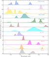 |
Fig. C.1 Laboratory spectra before (dashed) and after (solid) baseline correction. Each spectrum is normalized to its peak optical depth with offsets added for all ice mixtures. Details on the laboratory spectra are summarized in Table C.1. |
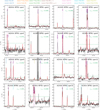 |
Fig. D.1 ALMA 3 mm spectra of SPR1 toward IRAS 18089 mm. In all panels, the observed ALMA spectrum extracted from the mm peak position is shown in black. The best-fit model obtained with xclass is shown in red taking into account all molecules. The 5σline level is highlighted by the horizontal green line. Vertical lines mark molecular transitions considered in the xclass fit with peak intensities of > 5σline. Optically thick lines excluded from the fit are gray-shaded. |
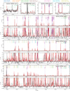 |
Fig. D.2 Same as Fig. D.1, but for SPR2. For the three broadband spws, an additional zoom in panel is shown to highlight the fainter lines. |
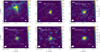 |
Fig. D.3 Molecular line emission maps of IRAS 18089. In all panels the ALMA line-integrated intensity (vLSR ± 5 km s-1) is shown in color and the gray contours are the ALMA 3 mm continuum with steps from 5, 10, 20, 40, 80, 160, and 320×σcont. The mm and MIR continuum peak positions are labeled and highlighted in red and pink. The red circle shows the aperture (1″ radius) used for spectra extraction toward the 3 mm continuum peak. A scale bar in the top left panel marks a spatial scale of 5 000 au. The ellipse in the bottom left and bottom right corner highlights the angular resolution of the line and continuum data. |
Molecular column densities in the ices and gas phase toward IRAS 18089.
Molecular column densities in the ices toward IRAS 18089 using different test setups.
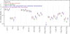 |
Fig. E.2 Comparison of the derived ice column densities of the final fit (Fig. 4) and additional tests (Fig. E.1). |
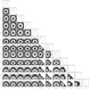 |
Fig. E.3 MCMC fit of the IRAS 18089 ice spectrum (Fig. 4) using the emcee package. The best-fit scaling factor (Eq. 4) is shown for each ice species. The corresponding ice column densities are summarized in Table E.1. |
All Tables
Molecular column densities in the ices toward IRAS 18089 using different test setups.
All Figures
|
Fig. 1 IRAS 18089 continuum images (left: ALMA 3 mm; center: JWST/MIRI-MRS 5 μm; right: JWST/MIRI-MRS 19 μm). In all panels, the black contours show the ALMA 3 mm continuum with steps from 5, 10, 20, 40, 80, 160, and 320×σcont. The mm and MIR continuum peak positions are labeled and highlighted in red and pink. The red circle shows the aperture (1" radius) used for spectra extraction toward the mm source. A scale bar in the top left panel marks a spatial scale of 5000 au. The ellipse in the bottom left corner highlights the angular resolution of each dataset. |
| In the text | |
|
Fig. 2 JWST/MIRI-MRS spectrum of IRAS 18089 mm. The observed MIR spectrum of the mm source is shown in black. The red line is the best-fit SED model taking into account emission by two black bodies (T1 = 410 K and T2 = 83 K) and absorption by dust and water ice. The data points that were included in the fit are highlighted by the blue dots. The green line shows the contribution by dust absorption and the purple line highlights the two black body emission components. Silicate features as well as main ice constituents (Whittet et al. 1996; Gibb et al. 2000; Yang et al. 2022; McClure et al. 2023) are labeled. The wavelength range with an increased noise (8.8-11.0 μm) is shaded in gray. |
| In the text | |
|
Fig. 3 Removal of gas phase lines and local continuum estimate. Top: contribution of gas phase SO2 emission (yellow) and CH4 absorption (red) lines estimated from the observed IRAS 18089 mm spectrum (gray). The corrected spectrum is shown in black. Bottom: corrected optical depth spectrum (black) and the local continuum interpolation (blue line). The red dots mark the guiding points used for the interpolation. The green dashed line shows the continuum interpolation based on a fifth-order polynomial (see Appendix E). |
| In the text | |
|
Fig. 4 Optical depth spectrum of IRAS 18089 mm after local continuum subtraction. The observed optical depth spectrum is presented in black, highlighting the absorption features by minor ice constituents. The total fit considering a mixture of ice species is shown by the thick dashed green line. The solid lines are contributions by each ice species (details on the laboratory data are summarized in Table C.1). |
| In the text | |
|
Fig. 5 Comparison of ice and gas phase abundances (relative to C2H5OH) toward IRAS 18089 mm. The crosses and squares mark ice and gas phase abundances, respectively. Blue, green, yellow, and red colors highlight COH-, N-, S-, and Si-bearing species. The column density of less abundant isotopologs (including 13C, 18O, 33S, and 34 S isotopes) were converted to their main isotopolog using relations by Wilson & Rood (1994) and Yan et al. (2023) with a Galactocentric distance of dgal=5.7kpc for IRAS 18089. |
| In the text | |
|
Fig. 6 Comparison of ice and gas phase abundances (relative to CH3OH) toward low- and high-mass hot cores. The crosses and squares mark ice and gas phase abundances, respectively. Blue, green, and red data points are IRAS 18089 mm (this work), IRAS 2A (Chen et al. 2024; Rocha et al. 2024), and B1-c (Chen et al. 2024). The pink data points are taken from the hot core model by Garrod et al. (2022) (the fast warm-up model at T=100 K; see their Fig. 10). |
| In the text | |
|
Fig. 7 Comparison of ice abundances (relative to H2O) toward low- and highmass protostars. The abundances toward the IRAS 18089 mm analyzed in this work is shown in blue. The results for the low-mass protostars B1-c (red) and IRAS 2A (orange) were taken from Chen et al. (2024). The high-mass protostar IRAS 23385 (green) and MIR peak of IRAS 18089 (pink) were analyzed in Rocha et al. (2024) and van Dishoeck et al. (2025), respectively. The ST6 source located in the LMC was studied by Sewiło et al. (2025) and is shown in purple. Upper limits are indicated by gray bars and triangle data points. |
| In the text | |
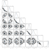 |
Fig. B.1 Uncertainty estimate of the IRAS 18089 SED model fit (Fig. 2) using the emcee package. |
| In the text | |
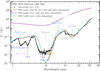 |
Fig. B.2 Same as Fig. 2, but including the 7.82 μm data point in the fit. |
| In the text | |
|
Fig. C.1 Laboratory spectra before (dashed) and after (solid) baseline correction. Each spectrum is normalized to its peak optical depth with offsets added for all ice mixtures. Details on the laboratory spectra are summarized in Table C.1. |
| In the text | |
|
Fig. D.1 ALMA 3 mm spectra of SPR1 toward IRAS 18089 mm. In all panels, the observed ALMA spectrum extracted from the mm peak position is shown in black. The best-fit model obtained with xclass is shown in red taking into account all molecules. The 5σline level is highlighted by the horizontal green line. Vertical lines mark molecular transitions considered in the xclass fit with peak intensities of > 5σline. Optically thick lines excluded from the fit are gray-shaded. |
| In the text | |
|
Fig. D.2 Same as Fig. D.1, but for SPR2. For the three broadband spws, an additional zoom in panel is shown to highlight the fainter lines. |
| In the text | |
|
Fig. D.3 Molecular line emission maps of IRAS 18089. In all panels the ALMA line-integrated intensity (vLSR ± 5 km s-1) is shown in color and the gray contours are the ALMA 3 mm continuum with steps from 5, 10, 20, 40, 80, 160, and 320×σcont. The mm and MIR continuum peak positions are labeled and highlighted in red and pink. The red circle shows the aperture (1″ radius) used for spectra extraction toward the 3 mm continuum peak. A scale bar in the top left panel marks a spatial scale of 5 000 au. The ellipse in the bottom left and bottom right corner highlights the angular resolution of the line and continuum data. |
| In the text | |
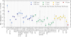 |
Fig. D.4 The same as Fig. 5, but abundances are computed relative to CH3OH. |
| In the text | |
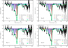 |
Fig. E.1 Same as Fig. 4, but including different tests for the ice fitting method. |
| In the text | |
|
Fig. E.2 Comparison of the derived ice column densities of the final fit (Fig. 4) and additional tests (Fig. E.1). |
| In the text | |
|
Fig. E.3 MCMC fit of the IRAS 18089 ice spectrum (Fig. 4) using the emcee package. The best-fit scaling factor (Eq. 4) is shown for each ice species. The corresponding ice column densities are summarized in Table E.1. |
| In the text | |
Current usage metrics show cumulative count of Article Views (full-text article views including HTML views, PDF and ePub downloads, according to the available data) and Abstracts Views on Vision4Press platform.
Data correspond to usage on the plateform after 2015. The current usage metrics is available 48-96 hours after online publication and is updated daily on week days.
Initial download of the metrics may take a while.