| Issue |
A&A
Volume 700, August 2025
|
|
|---|---|---|
| Article Number | A5 | |
| Number of page(s) | 26 | |
| Section | Planets, planetary systems, and small bodies | |
| DOI | https://doi.org/10.1051/0004-6361/202452560 | |
| Published online | 28 July 2025 | |
The KELT-7b atmospheric thermal-inversion conundrum revisited with CHEOPS, TESS, and additional data★
1
HUN-REN-ELTE Exoplanet Research Group,
Szent Imre h. u. 112,
9700
Szombathely,
Hungary
2
ELTE Gothard Astrophysical Observatory,
Szent Imre h. u. 112,
9700
Szombathely,
Hungary
3
Astronomical Institute, Slovak Academy of Sciences,
05960
Tatranská Lomnica,
Slovakia
4
Space Research Institute, Austrian Academy of Sciences,
Schmiedlstrasse 6,
8042
Graz,
Austria
5
INAF, Osservatorio Astrofisico di Torino,
Via Osservatorio, 20,
10025
Pino Torinese To,
Italy
6
INAF, Osservatorio Astrofisico di Catania,
Via S. Sofia 78,
95123
Catania,
Italy
7
Institute of Planetary Research, German Aerospace Center (DLR),
Rutherfordstrasse 2,
12489
Berlin,
Germany
8
Department of Physics, University of Warwick,
Gibbet Hill Road,
Coventry
CV4 7AL,
UK
9
Department of Astronomy, Stockholm University, AlbaNova University Center,
10691
Stockholm,
Sweden
10
European Space Agency (ESA), European Space Research and Technology Centre (ESTEC),
Keplerlaan 1,
2201
AZ
Noordwijk,
The Netherlands
11
Observatoire astronomique de l’Université de Genève,
Chemin Pegasi 51,
1290
Versoix,
Switzerland
12
Instituto de Astrofisica e Ciencias do Espaco, Universidade do Porto, CAUP, Rua das Estrelas,
4150-762
Porto,
Portugal
13
Departamento de Fisica e Astronomia, Faculdade de Ciencias, Universidade do Porto, Rua do Campo Alegre,
4169-007
Porto,
Portugal
14
Center for Space and Habitability, University of Bern,
Gesellschaftsstrasse 6,
3012
Bern,
Switzerland
15
Space Research and Planetary Sciences, Physics Institute, University of Bern,
Gesellschaftsstrasse 6,
3012
Bern,
Switzerland
16
Instituto de Astrofísica de Canarias, Vía Láctea s/n,
38200
La Laguna, Tenerife,
Spain
17
Departamento de Astrofísica, Universidad de La Laguna, Astrofísico Francisco Sanchez s/n,
38206
La Laguna, Tenerife,
Spain
18
Admatis,
5. Kandó Kálmán Street,
3534
Miskolc,
Hungary
19
Depto. de Astrofísica, Centro de Astrobiología (CSIC-INTA), ESAC campus,
28692
Villanueva de la Cañada (Madrid),
Spain
20
INAF, Osservatorio Astronomico di Padova,
Vicolo dell’Osservatorio 5,
35122
Padova,
Italy
21
Centre for Exoplanet Science, SUPA School of Physics and Astronomy, University of St Andrews,
North Haugh,
St Andrews
KY16 9SS,
UK
22
CFisUC, Departamento de Física, Universidade de Coimbra,
3004-516
Coimbra,
Portugal
23
Centre for Mathematical Sciences, Lund University,
Box 118,
221 00
Lund,
Sweden
24
Aix Marseille Univ, CNRS, CNES, LAM,
38 rue Frédéric Joliot-Curie,
13388
Marseille,
France
25
SRON Netherlands Institute for Space Research,
Niels Bohrweg 4,
2333
CA
Leiden,
The Netherlands
26
Centre Vie dans l’Univers, Faculté des sciences, Université de Genève,
Quai Ernest-Ansermet 30,
1211
Genève 4,
Switzerland
27
Leiden Observatory, University of Leiden,
PO Box 9513,
2300
RA
Leiden,
The Netherlands
28
Department of Space, Earth and Environment, Chalmers University of Technology, Onsala Space Observatory,
439 92
Onsala,
Sweden
29
Dipartimento di Fisica, Università degli Studi di Torino,
via Pietro Giuria 1,
10125
Torino,
Italy
30
National and Kapodistrian University of Athens, Department of Physics, University Campus, Zografos
157 84,
Athens,
Greece
31
Astrobiology Research Unit, Université de Liège,
Allée du 6 Août 19C,
4000
Liège,
Belgium
32
Department of Astrophysics, University of Vienna,
Türkenschanzstrasse 17,
1180
Vienna,
Austria
33
Institute for Theoretical Physics and Computational Physics, Graz University of Technology,
Petersgasse 16,
8010
Graz,
Austria
34
Konkoly Observatory, Research Centre for Astronomy and Earth Sciences,
1121
Budapest,
Konkoly Thege Miklós út 15–17,
Hungary
35
ELTE Eötvös Loránd University, Institute of Physics,
Pázmány Péter sétány 1/A,
1117
Budapest,
Hungary
36
Lund Observatory, Division of Astrophysics, Department of Physics, Lund University,
Box 118,
22100
Lund,
Sweden
37
IMCCE, UMR8028 CNRS, Observatoire de Paris, PSL Univ., Sorbonne Univ.,
77 av. Denfert-Rochereau,
75014
Paris,
France
38
Institut d’astrophysique de Paris, UMR7095 CNRS, Université Pierre & Marie Curie,
98bis blvd. Arago,
75014
Paris,
France
39
Astrophysics Group, Lennard Jones Building, Keele University,
Staffordshire
ST5 5BG,
UK
40
European Space Agency, ESA – European Space Astronomy Centre, Camino Bajo del Castillo s/n,
28692
Villanueva de la Cañada, Madrid,
Spain
41
Institute of Optical Sensor Systems, German Aerospace Center (DLR),
Rutherfordstrasse 2,
12489
Berlin,
Germany
42
Weltraumforschung und Planetologie, Physikalisches Institut, University of Bern,
Gesellschaftsstrasse 6,
3012
Bern,
Switzerland
43
Dipartimento di Fisica e Astronomia “Galileo Galilei”, Università degli Studi di Padova,
Vicolo dell’Osservatorio 3,
35122
Padova,
Italy
44
ETH Zurich, Department of Physics,
Wolfgang-Pauli-Strasse 2,
8093
Zurich,
Switzerland
45
Cavendish Laboratory,
JJ Thomson Avenue,
Cambridge
CB3 0HE,
UK
46
Institut fuer Geologische Wissenschaften, Freie Universitaet Berlin,
Maltheserstrasse 74-100,
12249
Berlin,
Germany
47
Institut de Ciencies de l’Espai (ICE, CSIC), Campus UAB, Can Magrans s/n,
08193
Bellaterra,
Spain
48
Institut d’Estudis Espacials de Catalunya (IEEC),
08860
Castelldefels (Barcelona),
Spain
49
Space sciences, Technologies and Astrophysics Research (STAR) Institute, Université de Liège,
Allée du 6 Août 19C,
4000
Liège,
Belgium
50
Institute of Astronomy, University of Cambridge,
Madingley Road,
Cambridge
CB3 0HA,
UK
51
HUN-REN-SZTE Stellar Astrophysics Research Group,
6500,
Baja,
Szegedi út, Kt. 766,
Hungary
★★ Corresponding author: This email address is being protected from spambots. You need JavaScript enabled to view it.
; This email address is being protected from spambots. You need JavaScript enabled to view it.
Received:
10
October
2024
Accepted:
21
May
2025
Abstract
Context. Early theoretical works suggested that ultrahot Jupiters have inverted temperature-pressure (T–P) profiles in the presence of optical absorbers, such as TiO and VO. Recently, an inverted T–P profile of KELT-7b was detected, in agreement with the predictions. However, the diagnosis of T–P inversions has always been recognized to be a model-dependent process.
Aims. We used the Characterising Exoplanet Satellite (CHEOPS), the Transiting Exoplanet Survey Satellite (TESS), and additional literature data to characterize the atmosphere of KELT-7b, rederive the T–P profile, provide a precise measurement of the albedo of KELT-7b, and search for a possible distortion in the precise CHEOPS transit light curve of the planet.
Methods. We first jointly fitted the CHEOPS and TESS data and measured the occultation depths in these passbands. The CHEOPS transits were also fitted with a model including the gravity-darkening effect. Emission and absorption retrievals were performed to characterize the atmosphere of KELT-7b. The albedo of the planet was calculated in the CHEOPS and TESS passbands.
Results. When adopting a thermochemical-equilibrium atmospheric composition, the emission retrievals return a non-inverted T–P profile, in contrast with previous results. When adopting a free-chemistry atmospheric parameterization, the emission retrievals return an inverted T-P profile with – likely unphysically – high concentrations of TiO and VO. The 3D general circulation model (GCM) supports a TiO-induced temperature inversion. We report for KELT-7b a very low geometric albedo of Ag = 0.05 ± 0.06, which is consistent with the heat distribution ϵ being close to zero and also consistent with a 3D GCM simulation, using magnetic drag (τdrag = 104 s). Based on the CHEOPS photometry, we are unable to place any meaningful constraint on the sky-projected orbital obliquity.
Conclusions. The choice of a free-chemistry approach or a thermochemical-equilibrium chemistry is the main factor determining the retrieval results. Free-chemistry retrievals generally yield better fits; however, assuming free chemistry risks adopting unphysical scenarios for ultrahot Jupiters, such as KELT-7b. We applied a coherent stellar variability treatment on TESS and CHEOPS observations, commensurate with the known stellar activity of the host star. Other observations of KELT-7b would also benefit from a coherent stellar variability treatment.
Key words: methods: observational / techniques: photometric / planets and satellites: atmospheres / planets and satellites: fundamental parameters / planets and satellites: individual
This article uses data from CHEOPS programmes CH_PR110016 and CH_PR100047.
© The Authors 2025
 Open Access article, published by EDP Sciences, under the terms of the Creative Commons Attribution License (https://creativecommons.org/licenses/by/4.0), which permits unrestricted use, distribution, and reproduction in any medium, provided the original work is properly cited.
This article is published in open access under the Subscribe to Open model. This email address is being protected from spambots. You need JavaScript enabled to view it. to support open access publication.
1 Introduction
Hot Jupiters are giant gaseous planets with short orbital periods and high equilibrium temperatures (Teq). In particular, ultrahot Jupiters, which have hot (Teq > 2000 K) and extended atmospheres (Bell & Cowan 2018), are ideal targets for both transmission and emission spectroscopy, owing to their atmospheric scale heights and brightness. Transmission spectroscopy, which measures the wavelength-dependent depth of the transit as the planet passes in front of its host star, is primarily sensitive to the atmospheric composition of the planet at the pressures of ~0.1–1000 mbar along the day-night terminator (Seager & Sasselov 2000; Brown 2001). Transmission spectroscopy is also sensitive to clouds and high-altitude hazes, which can mask atmospheric absorption features by acting as a gray opacity source (Fortney 2005; Helling et al. 2019). This technique and its variants have been used to detect several atomic and molecular species in exoplanetary atmospheres, such as Na (Charbonneau et al. 2002; Snellen et al. 2008; Redfield et al. 2008; Nikolov et al. 2018), K (Sing et al. 2015; Wilson et al. 2015), TiO (Sedaghati et al. 2017), H2O (Deming et al. 2013; Kreidberg et al. 2014), CO (Snellen et al. 2010), CO2 (Swain et al. 2009; Madhusudhan et al. 2023; JWST Transiting Exoplanet Community Early Release Science Team 2023), CH4 (Swain et al. 2008, 2009; Bell et al. 2023; Madhusudhan et al. 2023), NH3 (MacDonald & Madhusudhan 2017), SO2 (Tsai et al. 2023; Powell et al. 2024; Dyrek et al. 2024), and H2S (Fu et al. 2024).
We can also characterize the thermal emission spectra of transiting planets (Barman et al. 2005; Burrows et al. 2005; Seager et al. 2005) by measuring the wavelength-dependent depth of the secondary eclipse (occultation) as the planet passes behind its host star (see, e.g., Kreidberg et al. 2014; Stevenson et al. 2014b; Haynes et al. 2015; Line et al. 2016; Beatty et al. 2017; Evans et al. 2017; Mikal-Evans et al. 2019; Mansfield et al. 2018; Edwards et al. 2020, or Pluriel et al. 2020). Unlike transmission spectroscopy, which probes the atmosphere near the day-night terminator, these emission spectra tell us about the global properties of the planet’s dayside atmosphere. They are sensitive to both the dayside composition and the vertical temperature-pressure (T-P) profile, which determines if the molecular absorption features are seen in absorption or emission. In terms of radiative transport only, the emergence of thermal inversions can be understood as being controlled by the ratio of opacity at visible wavelengths (which controls the depth to which incident flux penetrates) to the opacity at thermal infrared wavelengths (which controls the cooling of the planetary atmosphere). Generally, if the optical opacity is high at low pressure, leading to absorption of stellar flux high in the atmosphere, and the corresponding thermal infrared opacity is low, the upper atmosphere will have less efficient cooling, leading to elevated temperatures at low pressure (Madhusudhan et al. 2014).
Early theoretical works suggested that ultrahot Jupiters have inverted T-P profiles in the presence of optical absorbers, such as TiO and VO (Hubeny et al. 2003; Fortney et al. 2008). H− is also considered as a potential absorber, capable of causing thermal inversion (see, e.g., Lothringer et al. 2018). The strong opacity of TiO and VO could result in thermal inversions, that is, rising temperatures with higher altitudes. Conversely, several studies explored mechanisms explaining why TiO might not play a role in the upper atmosphere (Spiegel et al. 2009; Madhusudhan 2012; Parmentier et al. 2013). Thermal inversions were found, for example, in the ultrahot Jupiters WASP-33b (Haynes et al. 2015), WASP-121b (Evans et al. 2017), WASP-103b (Kreidberg et al. 2018), KELT-9b (Pino et al. 2020), and KELT-7b (Pluriel et al. 2020). The ultrahot Jupiter WASP-12b is an exception; it shows no signs of TiO absorption or temperature inversion (Sing et al. 2013; Akinsanmi et al. 2024). This is in disagreement with the predictions, which emphasize the importance of such detections. Observations of hot Jupiters with Teq < 2000 K, WASP-43b (Stevenson et al. 2014b) and HD 209458b (Line et al. 2016; Santos et al. 2020), detected non-inverted T-P profiles, in agreement with the predictions of Hubeny et al. (2003) and Fortney et al. (2008). However, the diagnosis of temperature inversions has always been recognized to be a model-dependent process (Madhusudhan et al. 2014).
Furthermore, the observed occultation depth can be translated into a geometric albedo if only reflected starlight is measured (Heng & Demory 2013), or if thermal emission contribution is taken into account (Wong et al. 2020, 2021). The geometric albedo Ag is a wavelength-dependent quantity, defined as the albedo of the planet at full phase (Russell 1916; Seager 2010). It determines how much starlight enters the planet’s atmosphere without being reflected at its top. The first confirmed secondary-eclipse detections of the planets HD 209458b (Deming et al. 2005) and TrES-1b (Charbonneau et al. 2005) were reported with the Spitzer Space Telescope (Werner et al. 2004). Dedicated exoplanet space-based optical telescopes, this means, the Kepler space telescope (Borucki et al. 2010), the Transiting Exoplanet Survey Satellite (TESS; Ricker et al. 2014), and the Characterising Exoplanet Satellite (CHEOPS; Benz et al. 2021; Fortier et al. 2024) were also frequently used to measure the secondary eclipses and geometric albedos of transiting exoplanets (see, e.g., Heng & Demory 2013; Angerhausen et al. 2015 or Esteves et al. 2015 in the case of Kepler, Wong et al. 2020, 2021 in the case of TESS, and Lendl et al. 2020b; Brandeker et al. 2022; Hooton et al. 2022; Deline et al. 2022; Scandariato et al. 2022 or Krenn et al. 2023 in the case of CHEOPS). The unprecedented precision of these observations reveals that hot Jupiters have, in general, low geometric albedos, which means Ag < 0.3 (Cowan & Agol 2011; Esteves et al. 2013), in some cases, Ag < 0.1 (Angerhausen et al. 2015; Esteves et al. 2015).
In this work, we selected the KELT-7 system (Bieryla et al. 2015) as a subject of our follow-up. KELT-7b has a short orbital period of ~2.734 d, a mass of ~1.28 MJup, and a radius of ~1.496 RJup. This exoplanet is an ultrahot Jupiter with Teq = 2028 ± 17 K (Tabernero et al. 2022b) transiting a bright (V = 8.54 mag) F2V-type star (see Sect. 3 for further details). When discovered, this host was the fifth most massive, fifth hottest, and the ninth brightest star known to host a transiting planet. Therefore, KELT-7b is an ideal target for atmospheric characterization. Recent works also focus on the atmosphere of KELT-7b. Pluriel et al. (2020) detect strong absorption features in the transmission spectrum indicative of H2O and H−. On the other hand, the emission spectrum lacks strong absorption features. The analysis reveals temperature inversion. Later, Stangret et al. (2022) searched for absorption features of a broad range of atomic and molecular species in a sample of six hot Jupiters based on high-resolution transmission spectroscopy. The nondetection in the case of KELT-7b is explained by stellar pulsations and the Rossiter-McLaughlin effect. Similarly, Tabernero et al. (2022b) are only able to determine upper limits of 0.08–1.4% on the presence of Hα, Li I, Na I, Mg I, and Ca II.
Furthermore, the rapid rotation of the host star, with v sin Is = 71.4 ± 0.2 km s−1 (Tabernero et al. 2022b), makes this system even more interesting. The rapid rotation at early-type stars leads to an oblate shape of the star and induces an equator-to-pole gradient in the effective temperature, called gravity darkening (von Zeipel 1924a,b). The so-called von Zeipel theorem predicts that the flux emitted from the surface is proportional to the local effective gravity, and thus the effect induces cooler temperatures at a rapidly rotating star’s equator and hotter temperatures at the poles. If an exoplanet transits a rapidly rotating star, distorted transit light curves are expected, as was predicted by Barnes (2009). If such asymmetries are measured (see, e.g., Szabó et al. 2011; Lendl et al. 2020b; Hooton et al. 2022; Deline et al. 2022 or Jones et al. 2022), this can be used to determine the sky-projected angle λ between the stellar rotational axis and the planet orbit normal; that is, we can detect the spinorbit misalignment. In addition, the stellar inclination Is can be derived, and thus the true misalignment Ψ is possible to obtain.
We observed KELT-7b photometrically using the CHEOPS space observatory. In addition, we used TESS photometric data and literature data (see Sect. 2). We aim to characterize the atmosphere of the planet mainly via emission spectroscopy, to provide a precise measurement of the albedo of KELT-7b, and to search for a possible distortion in the CHEOPS transit light curve of the planet. The paper is organized as follows. In Sect. 2, we provide a brief description of observations and data reduction. In Sect. 3, we summarize the most important stellar parameters based on Tabernero et al. (2022b). The data analysis, including light-curve fitting, secondary eclipse detection, and search for transit asymmetry, is described in Sect. 4. Atmosphere modeling of KELT-7b is the subject of Sect. 5. In Sect. 6, we discuss the results of the atmosphere modeling. We conclude with the results in Sect. 7.
Log of CHEOPS photometric observations of KELT-7 used in this work.
2 Observations and data reduction
2.1 CHEOPS data
CHEOPS performed a total of 14 observations (visits) of KELT-7 between October 2021 and January 2023 (see Table 1 for further details). The secondary eclipse observations were performed within CHEOPS programme CH_PR110016, while the transits of KELT-7b were observed under programme CH_PR100047. The CHEOPS observations are available as subarray data products (Benz et al. 2021) at a cadence equal to the exposure time (26.0 s for occultation and 28.0 s for transit observations). The subarrays contain a circular region around the target with a radius of 100 pixels. Aperture photometry is available for the subarrays via the official CHEOPS Data Reduction Pipeline (DRP; Hoyer et al. 2020). It performs several image corrections, including bias, dark, and flat corrections, contamination estimation, and background-star correction. We processed all CHEOPS observations with the DRP version 14.1.2 using an aperture radius of 24 pixels.
In general, CHEOPS observations are affected by instrumental noise such as stray light from the Earth and the Moon (Moon glint), smearing effects, or spacecraft jitter. The flux measurements usually show a particularly strong correlation with the spacecraft roll angle (see, e.g., Lendl et al. 2020b; Bonfanti et al. 2021). The spacecraft rotates around itself exactly once every orbit. Therefore, the roll-angle parameter is directly linked to the orbital position of the spacecraft. Instrumental noise must be accounted for during the data analysis to identify the transit and occultation signals of the planet (see Sect. 4). Before performing the data analysis, we removed all points flagged by the DRP; this includes those points contaminated, for example, by cosmic rays. We also removed points with peculiarly high backgrounds by removing any points with a background larger than four times the median background value, as well as points with unusually high pointing offsets by removing all points with a centroid offset of more than 1 pixel. Finally, we also removed points with a smearing estimate larger than 3 × 10⁻⁵. In the case of the occultation data, we also performed sigma clipping and removed all points with median absolute deviation (MAD) higher than four to discard outliers.
2.2 TESS data
In this work, we used TESS photometric data of KELT-7 from Sectors 19, 43, 44, 45, 59, 71, and 73 at 2 min cadence. The TESS photometric baseline, therefore, spans from November 2019 to January 2024 (see Table 2 for further details). In the case of Sectors 59, 71, and 73, there are also 20 s cadence data available, which, however, were not used in this work. In our analysis, we used the Pre-search Data Conditioning Simple Aperture Photometry (PDCSAP) flux, provided by the Science Processing Operations Center (SPOC) pipeline (Smith et al. 2012; Stumpe et al. 2012, 2014; Jenkins et al. 2016). Contrary to the Simple Aperture Photometry (SAP) flux, the PDCSAP light curve product has long-term trends removed from the data using Co-trending Basis Vectors (CBVs). The pipeline attempts to remove systematic artifacts while keeping planetary transits intact. Therefore, PDCSAP flux has fewer systematic trends and is specifically intended for detecting exoplanets. In principle, the PDCSAP light curve product should also be corrected for light dilution. The data were downloaded from the Mikulski Archive for Space Telescopes1 (MAST). The average uncertainty of the 109 739 data points is 400 ppm. We did not apply outlier removal in the TESS dataset.
Log of TESS photometric observations of KELT-7 used in this work.
2.3 Additional data
During the analysis, we also used the following literature data. Martioli et al. (2018) present near-infrared high-precision photometric observations of secondary eclipses for eight transiting hot Jupiters, including KELT-7b. The observations were carried out using the Wide-field InfraRed Camera (WIRCam) instrument (Puget et al. 2004) installed on the Canada-France-Hawaii Telescope (CFHT). KELT-7b was observed using the Kcont filter (at a wavelength of λ ~ 2.2 μm). The observations reveal an occultation depth of Docc,CFHT = 400 ± 120 ppm. However, we later discarded this data point from the analysis, because it was very probably inconsistent with any tested model (see Fig. 7). Unfortunately, ground-based observations are often affected by strong correlated noise (see, e.g., Hooton et al. 2019). Garhart et al. (2020) report transit depth and occultation depth measurements for a sample of 36 transiting hot Jupiters observed at λ ~ 3.6 μm and λ ~ 4.5 μm using the Spitzer space telescope (Werner et al. 2004) and its InfraRed Array Camera (IRAC) instrument (Fazio et al. 2004). For KELT-7b, the authors report transit depths of Dtra,Spitzer,3.6 = 7925 ± 62 ppm and Dtra,Spitzer,4.5 = 8092 ± 36 ppm. The observed occultation depths of KELT-7b are Docc,Spitzer,3.6 = 1688 ± 46 ppm and Docc,Spitzer,4.5 = 1896 ± 57 ppm. Finally, we also used literature transit depth and occultation depth data obtained from 25 spectral bins (λ ~ 1.12–1.63 μm) using the Wide Field Camera 3 (WFC3) instrument (Leckrone et al. 1998) installed on the Hubble Space Telescope (HST), which were published by Pluriel et al. (2020).
3 The planet’s host star
Properties of the planet’s host star, KELT-7, were obtained by Tabernero et al. (2022b) only recently. The authors employed the SteParSyn code2 (Tabernero et al. 2022a) to retrieve the stellar atmospheric parameters and their associated uncertainties. Using these stellar parameters, they calculated the age of the star, its mass, and its radius with the PARAM web interface3 (da Silva et al. 2006), and the PARSEC stellar evolutionary tracks and isochrones (Bressan et al. 2012). During the joint fit and eclipse detection (see Sect. 4.4), we used stellar parameters derived by these authors, including the stellar radius Rs = 1.712 ± 0.037 R⊙, the stellar mass Ms = 1.517 ± 0.022 M⊙, the effective temperature Teff = 6699 ± 24 K, the surface gravity log g = 4.15 ± 0.09 dex, and metallicity [Fe/H] = 0.24 ± 0.02 dex. The age of the star is estimated to be 1.2 ± 0.7 Gyr. Further stellar parameters are listed in Table 1 in Tabernero et al. (2022b).
4 Data analysis
4.1 CHEOPS instrumental noise
CHEOPS flux measurements are known to often show a strong correlation with the spacecraft roll angle (see Sect. 2.1). However, in the case of the KELT-7 CHEOPS observations, we do not find such a strong correlation. For this reason, we refrained from using a more elaborate roll-angle correction and only used a first-order linear model of the sine and cosine of the roll-angle parameter to remove roll-angle-related trends. We also added a first-order linear detrending model on the offsets of the x- and y-centroid positions relative to their mean values. All of the linear detrending vectors were fitted simultaneously with the astrophysical model.
4.2 Stellar activity
Tabernero et al. (2022b) show that KELT-7 TESS light curves are heavily affected by stellar activity due to the rapid rotation of the star. Accordingly, the authors obtain a stellar rotation period of Prot,s = 1.38 ± 0.05 d. Following their findings, we also observe periodic flux changes in the TESS data that most likely are caused by stellar activity (see Figs. A.4 and A.5; left panels). We note that the same variability signal can be seen in both the PDCSAP and SAP flux. The effects of stellar activity must be accounted for in both TESS and CHEOPS observations when deriving the transit and eclipse parameters. To properly model the stellar noise, we employed a Gaussian process (GP) model. It was built using a Simple Harmonic Oscillator (SHO) kernel based on celerite4 models (Foreman-Mackey et al. 2017). The kernel is parameterized with an undamped angular frequency of the oscillator ω0, a quality factor Q, and the amplitude of the power spectral density S0 at ω = ω0 (Foreman-Mackey et al. 2017; Foreman-Mackey 2018):
![Mathematical equation: $\[S(\omega)=\sqrt{\frac{2}{\pi}} \frac{S_0 \omega_0^4}{\left(\omega^2-\omega_0^2\right)^2+\omega_0^2 \omega^2 / Q^2}.\]$](/articles/aa/full_html/2025/08/aa52560-24/aa52560-24-eq1.png) (1)
(1)
The parameters ω0 and Q can also be expressed via the undamped period of the oscillator ρSHO and the damping timescale of the process τSHO:
![Mathematical equation: $\[\rho_{\mathrm{SHO}}=\frac{2 \pi}{\omega_0},\]$](/articles/aa/full_html/2025/08/aa52560-24/aa52560-24-eq2.png) (2)
(2)
![Mathematical equation: $\[\tau_{\mathrm{SHO}}=\frac{2 Q}{\omega_0}.\]$](/articles/aa/full_html/2025/08/aa52560-24/aa52560-24-eq3.png) (3)
(3)
To model stellar activity, the parameters ρSHO, τSHO, and S0 can be interpreted as the stellar rotation period Prot,s, the characteristic damping timescale of star spot dissipation τdis, and the amplitude of the activity-induced variations S0, respectively. Both Prot,s and τdis are independent of time of observation and observed filter, while S0 depends on the observed wavelength range. Therefore, we assumed a common Prot,s and τdis across all observations while accounting for independent S0 parameters for TESS and CHEOPS observations. We also added a white-noise term σ per instrument. To constrain the GP parameter ρSHO (i.e., the proxy of the stellar rotation period), we analyzed the periodogram of TESS Sector 59 (see left panel of Fig. 1). We find the maximum peak of the periodogram at 1.368 d. Assuming a Gaussian distribution to fit for the width of the peak we defined a prior on Prot,s of 1.368 ± 0.030 d and translated it to a prior on ω0 of 4.59 ± 0.10 following Eq. (2). A similar peak can be found when analyzing the periodograms of all the other TESS sectors. We note that this prior on the stellar rotation period is very similar to half of the orbital period of the planet, which would be 1.3674 d. To ensure that this peak in the periodograms is not caused by the planet, but due to the stellar variability, we also checked the periodograms of the TESS sectors after removing the transits and occultations, which still contain the identical peak (see middle panel of Fig. 1). Additionally, we also note that the final fitted rotational period of the star is 1.320 ± 0.020 d (see Sect. 4.4), which is more than 3σ different from half of the orbital period of the planet.
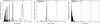 |
Fig. 1 Periodograms of KELT-7 TESS PDCSAP observations. The blue dashed line represents the fitted orbital period of the planet. The red dashed line represents the median value of the prior imposed on the stellar rotational period. Left panel: periodogram of TESS Sector 59 raw data, which was used to determine the prior. Middle panel: periodogram of the residuals of TESS Sector 45 data after removal of the transits and occultations. Right panel: periodogram of the residuals of TESS Sector 45 data. |
4.3 Planetary model and limb darkening law
To fit the planetary model, we adopted wide uniform priors on the impact parameter b, the total transit duration Wtra, the reference mid-transit time Tc, and the orbital period Porb. The values of the adopted priors are listed in Table 3. We also fitted individual planet-to-star radius ratios and occultation depths for each of the observed filters (TESS and CHEOPS), which were also subject to uniform priors. We did not incorporate ellipsoidal variation and Doppler beaming into our planetary model, as their theoretical estimates are only a few ppm, and therefore do not significantly impact our model fitting. Additionally, based on the TESS phase-curve analysis, we found insignificant nightside flux estimates, which means that we could not account for any meaningful heat-distribution efficiency. To account for limb darkening (LD), we adopted a quadratic LD law. We computed theoretical LD coefficients, including their uncertainties for KELT-7 using the LDCU Python package (see Table 3). LDCU5 is a modified version of the Python routine implemented by Espinoza & Jordán (2015) that computes the LD coefficients and their corresponding uncertainties using a set of stellar intensity profiles that account for the uncertainties in the stellar parameters. The stellar intensity profiles are generated based on two libraries of synthetic stellar spectra: ATLAS (Kurucz 1979) and PHOENIX (Husser et al. 2013).
4.4 Joint fit and eclipse detection
To retrieve the secondary eclipse depths, we proceeded by jointly fitting all planetary parameters, the basis vectors of the linear-detrending models for CHEOPS, and the GP parameters within a Markov chain Monte Carlo (MCMC) framework, using the COde for transiting exoplaNet ANalysis 3 (CONAN3) Python package (Lendl et al. 2017, 2020a). We used 40 chains, with each chain performing 30 000 steps, of which the first 10 000 steps were discarded. We used the Gelman-Rubin test (Gelman & Rubin 1992) to check the convergence of our fit. We also analyzed the periodograms of the residuals to ensure that the combined variability and planetary model can account for all periodic variations in the data (see right panel of Fig. 1). The medians and 1σ confidence intervals of the fitted parameters, including the secondary eclipse depths, are listed in Table 3. The derived parameters are presented in Table 4. The phase-folded and fitted CHEOPS and TESS light curves are depicted in Fig. 2. Supplementary figures can be found in Appendix A.
Finally, we performed a test fit – reran the described joint-fit procedure, keeping everything identical except for the stellar parameters. In this case, we applied the stellar parameters published by Bieryla et al. (2015) – and used previously by Pluriel et al. (2020) – instead of the stellar parameters presented by Tabernero et al. (2022b). We tested the impact of the change on the fitted parameters. We do not detect any significant difference. The fitted parameters are well within the 1σ uncertainties, similarly to the two sets of stellar parameters, which are also consistent with each other within 1σ of their uncertainties.
4.5 Search for transit asymmetry
Based on spectroscopy, Bieryla et al. (2015) find that the normal of the orbit of the planet is likely to be well-aligned with the stellar spin axis, with a projected spin-orbit angle of λ = 9.7 ± 5.2 deg. Later, Zhou et al. (2016) confirm the spinorbit alignment of the system with an improved value of λ = 2.7 ± 0.6 deg. Tabernero et al. (2022b) obtain a projected spinorbit angle of λ = −10.55 ± 0.27 deg, and a 3D spin-orbit angle of Ψ = 12.4 ± 11.7 deg.
Given the rapid rotation of KELT-7 (see Sect. 1), we tried fitting the transit photometric data from CHEOPS with a model that includes the gravity-darkening effect. We used the Transit and Light Curve Modeller code (TLCM; Csizmadia 2020; Csizmadia et al. 2023), which was previously used to model gravity-darkened transits in the WASP-189 (Lendl et al. 2020b), MASCARA-1 (Hooton et al. 2022), WASP-33 (Kálmán et al. 2022), and KELT-20 (Singh et al. 2024) systems. Alongside the usual parameters to describe the transit (Porb, Rp,CHEOPS/Rs, a/Rs, b, and the LD coefficients), we fitted for the stellar inclination Is, and longitude of the node Ωs of the stellar rotation axis. To account for the systematic noise in the light curve, including the roll-angle effect, we tried three different approaches, each of which introduces additional fitting parameters. The first approach was to fit the roll-angle effect with two sine and two cosine terms per transit. The second was to rely solely on the wavelet method of red-noise fitting (Csizmadia et al. 2023; Carter & Winn 2009), which involves fitting for the red- and white-noise levels of the light curve, σr and σw. Finally, we tried a combination of the previous two approaches, employing both trigonometric terms and wavelets.
We obtain consistent results from all three methods of dealing with correlated noise in the light curves. The transit parameters resulting from these fits are also in good agreement (within 1σ) with those presented in Table 3. We find no significant difference in the quality of the fits obtained from TLCM with and without gravity darkening. In other words, we find no evidence of significant transit asymmetry. We find Is = 86 ± 25 deg, and we are unable to place any meaningful constraint on the sky-projected orbital obliquity (λ = 8 ± 105 deg6.
Fitted CONAN3 parameters of the KELT-7 planetary system.
Derived CONAN3 parameters of the KELT-7 planetary system.
5 Atmosphere modeling
The observed emission of KELT-7b, as measured by CHEOPS and TESS, may include contributions from both reflected stellar light (characterized by its albedo properties) and thermal emission from the planet (characterized by its thermal structure and composition). To distinguish between reflected and thermal signals, we focused on the thermal emission of KELT-7b using atmospheric retrievals from its infrared emission observations (HST and Spitzer, see Sect. 2.3). To avoid biasing the results with data points affected by reflected light, which is not modeled in this case, we excluded the CHEOPS and TESS occultation observations from the retrieval (see Table 3). To perform a robust assessment of our atmospheric analysis, we conducted Bayesian retrievals using two independent frameworks. To evaluate the impact of our model assumptions and to compare our findings with those in the literature (Pluriel et al. 2020; Changeat et al. 2022), we systematically tested multiple model assumptions by applying equivalent assumptions across both frameworks, adapted where necessary to their respective implementations. Throughout our retrieval analyses, we assumed the system parameters reported by Bieryla et al. (2015) and used by Pluriel et al. (2020), unless otherwise specified.
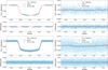 |
Fig. 2 Phase-folded, detrended, and binned CHEOPS (top panels) and TESS (bottom panels) transit (left panels) and occultation (right panels) light curves of KELT-7b, overplotted with the best-fitting CONAN3 model. Residuals are also shown. |
5.1 Atmospheric retrieval with PYRAT BAY
To characterize the atmospheric properties of KELT-7b, we employed the open-source PYRAT BAY modeling framework (Cubillos & Blecic 2021). The PYRAT BAY package combines parameterized atmospheric modeling, spectral synthesis, and Bayesian posterior sampling, which together constrain the planetary atmospheric profiles based on the occultation observations. In this work, we modeled the dayside KELT-7b atmosphere as a one-dimensional (1D) profile as a function of pressure, adopting a temperature profile (Madhusudhan & Seager 2009). For composition, we tested two alternatives: one following the free-chemistry parameterization (i.e., modeling the abundance of each absorber as a constant-with-altitude free parameter), and another one assuming thermochemical equilibrium consistent with the temperature profile (Cubillos et al., in prep.). We parameterized the composition with two free parameters that determine the atmospheric metallicity (abundance of all metal elements, relative to solar [M/H]) and the carbon elemental abundance (relative to oxygen, C/O).
The radiative-transfer calculation considered opacities from the main molecular species expected for hot Jupiters, including CO (Li et al. 2015), CO2 (Rothman et al. 2010), CH4 (Hargreaves et al. 2015), H2O (Polyansky et al. 2018), HCN (Harris et al. 2006, 2008), NH3 (Yurchenko 2015; Coles et al. 2019), FeH (Bernath 2020), TiO (McKemmish et al. 2019), and VO (McKemmish et al. 2016). We pre-processed the larger ExoMol line lists with the REPACK algorithm (Cubillos 2017) to extract the dominant transitions before sampling them to a fixed grid at a resolving power of 15 000. The code also included Rayleigh scattering by H, H2, and He (Kurucz 1970); H2–H2 and H2–He collision-induced absorption (Borysow et al. 1988; Borysow & Frommhold 1989; Borysow et al. 1989, 2001; Borysow 2002; Jørgensen et al. 2000); and H− continuous absorption (John 1988). For transmission geometry, we also included the opacity from the Na and K resonant lines (Burrows et al. 2000). The posterior sampling was handled by the MC3 package (Cubillos et al. 2017), using the Nested-sampling algorithm (via PYMULTINEST, Feroz et al. 2009; Buchner et al. 2014) with 2000 live points.
5.2 Atmospheric retrieval with PLATON
To test the robustness of our atmospheric characterization and its sensitivity to different modeling assumptions, we employed a second atmospheric retrieval tool. We adopted the open-source PLATON software, version 6.2 (Zhang et al. 2025). For the eclipse retrieval, we assumed a cloud-free atmosphere using the default opacities provided by PLATON at a resolution of R = 20 000, which include gas and collision-induced absorption from H2O, CO, CO2, CH4, TiO, VO, Na, K, and FeH (see the aforementioned release paper for further details). We also included H− bound-free and free-free continuous absorption given the high expected temperature of the planetary atmosphere (see, e.g., John 1988; Arcangeli et al. 2018).
The emission spectroscopy retrievals were carried out for both the thermochemical-equilibrium (where abundances are described through metallicity [M/H] and the C/O ratio parameters) and the free-chemistry scenarios (where species abundances are directly fit as constant-with-altitude volume mixing ratios). We adopted Madhusudhan & Seager (2009)’s parameterization for the temperature profile. To sample the parameter posterior distributions, we used PYMULTINEST (Feroz & Hobson 2008; Feroz et al. 2009, 2019; Buchner et al. 2014) with the uniform priors shown in Table 5, and 1000 live points. For the thermochemical equilibrium scenario, we explored the full metallicity and C/O ratio ranges allowed by PLATON’s model grid, while in the free chemistry scenario, all absorbers were assigned a prior on the volume mixing ratio ranging from 10−12 to 10−2.
Priors and posterior parameter estimations (median and 68% credible intervals) for the atmospheric retrievals.
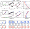 |
Fig. 3 KELT-7b atmospheric retrieval of the infrared occultations. Top left panel: retrievals assuming thermochemical equilibrium with PYRAT BAY (blue) and PLATON (pink). The solid curves with shaded areas show the median and 1σ span of the posterior model spectra, displayed at a resolution of R = 150. The black circle markers with error bars show observations used to constrain the models (HST and Spitzer). The green square markers show the CHEOPS and TESS occultation depths (not used as retrieval constraints). The diamond markers show the model spectra integrated over the observing bands. The insets zoom in on the regions probed by the observations. Top right panel: retrieved T–P profiles for each retrieval code (median and 1σ span from the posterior distribution, same color coding as previous panel). The gray hatched area denotes the range of pressures probed by the observations. Middle panels: same as above, but for the free-chemistry retrievals. Bottom panels: posterior distribution of the atmospheric composition parameters (same color coding as above). The labels on top of each posterior show the mean and 1σ uncertainties for each parameter posterior (denoted with a dashed line and shaded area, respectively). Some parameters have been omitted from this figure (see Table 5 for the full list of free parameters). |
5.3 Occultation retrieval results
Figure 3 shows the PYRAT BAY and PLATON retrieved occultation spectra, T-P profiles, and parameter posteriors (see Table 5 as well). We find that both retrieval codes produce consistent results when subjected to the same set of assumptions. When assuming a thermochemical-equilibrium atmospheric composition, the retrievals return a non-inverted T-P profile (probing mainly the 1–10−4 bar range) with a composition characterized by a C/O ratio greater than one (C/O > 1.1, at the 3σ lower boundary) and a super-solar metallicity in the 170–400× solar range ([M/H] = ![Mathematical equation: $\[2.6_{-0.5}^{+0.3}\]$](/articles/aa/full_html/2025/08/aa52560-24/aa52560-24-eq95.png) for PYRAT BAY, [M/H] = 2.2 ± 0.5 for PLATON). The main driver for this behavior is the relatively weak H2O absorption feature at 1.4 μm, since a C/O > 1 scenario leads to a depletion of H2O abundance. In contrast, when adopting a free-chemistry atmospheric parameterization, the retrievals return an inverted T-P profile between 0.1–10−6 bar. In this case, the strong optical absorbers TiO and VO are the only species with well-constrained abundances, albeit at – likely unphysically – high concentrations. The retrievals constrain the water abundance (volume mixing ratio) to less than ~10–100 ppm. Once again, this may be due to the absence of a clear H2O absorption feature at 1.4 μm.
for PYRAT BAY, [M/H] = 2.2 ± 0.5 for PLATON). The main driver for this behavior is the relatively weak H2O absorption feature at 1.4 μm, since a C/O > 1 scenario leads to a depletion of H2O abundance. In contrast, when adopting a free-chemistry atmospheric parameterization, the retrievals return an inverted T-P profile between 0.1–10−6 bar. In this case, the strong optical absorbers TiO and VO are the only species with well-constrained abundances, albeit at – likely unphysically – high concentrations. The retrievals constrain the water abundance (volume mixing ratio) to less than ~10–100 ppm. Once again, this may be due to the absence of a clear H2O absorption feature at 1.4 μm.
We tested a range of configurations to explore the dependence of the retrieval results on the model assumptions. We performed three additional comparisons: (1) retrievals adopting the system parameters from this work and those used in Pluriel et al. (2020), (2) retrievals employing a different thermal profile parameterization (Guillot 2010), and (3) retrievals including only the molecular absorbers of Pluriel et al. (2020) versus a larger set of absorbers (see Sect. 5.1). None of these tests led to qualitatively different retrieval results.
Pluriel et al. (2020) and Changeat et al. (2022) have previously presented atmospheric retrieval analyses of KELT-7b based on the HST/WFC3 and Spitzer occultations. Adopting a free-chemistry parameterization, they both find an inverted T–P profile, a nondetection of H2O, and a detection of H− absorption. Changeat et al. (2022) further performed retrievals assuming equilibrium chemistry, finding solar to super-solar metallicities, C/O ratios greater than one, and a different thermal structure. These findings are well in agreement with our results, with the main difference being the optical absorber found for the free-chemistry parameterization. This is not unexpected – as both TiO and VO or H− optical absorbers are not strongly constrained by the near-infrared observations, in both scenarios, they contribute to a higher brightness temperature at the blue end of the WFC3 band. Thus, our comparison tests and the agreement with previous analyses from the literature lead us to conclude that the choice of free or thermochemical-equilibrium chemistry is the main factor driving the retrievals to different atmospheric scenarios.
We note that the free-chemistry retrievals generally yield better fits to the observations than the thermochemical-equilibrium retrievals. However, assuming free constant-with-altitude abundances risks adopting scenarios at odds with plausible physical conditions. The dayside atmosphere of ultrahot Jupiters similar to KELT-7b is expected to reach temperatures exceeding 2000 K. Since disequilibrium-chemistry processes, such as photochemistry and transport-induced quenching, become less and less important with increasing effective temperature, at these extreme temperatures the chemical reaction rates are fast enough to overcome the effect of disequilibrium chemistry (Kopparapu et al. 2012; Moses 2014; Madhusudhan et al. 2016; Venot et al. 2018). Thermochemical equilibrium is therefore the expected assumption to model the dayside atmospheric composition of planets similar to KELT-7b and their resulting emission spectra. If disequilibrium chemistry occurs at all (e.g., photochemistry), it would occur at high altitudes above the pressures probed by the observations presented in this work, and thus the modeled emission spectra of planets similar to KELT-7b would not be significantly impacted (Shulyak et al. 2020). In contrast, thermochemical-equilibrium calculations indicate that we expect a strong variation in abundances with altitude at the pressures where H2 dissociates into H, which can occur precisely at the pressures probed by near-infrared observations. In the specific case of KELT-7b, the free-chemistry retrievals point to high abundances of TiO (this work) or e− (Pluriel et al. 2020; Changeat et al. 2022), which are orders of magnitude above expected values from self-consistent chemical models. The suboptimal thermochemical-equilibrium fit suggests that there may be missing physics in these retrieval models, which may be resolved with the availability of improved data.
Lastly, we must consider that combining multi-epoch observations can lead to biases in the atmospheric interpretation due to stellar activity, instrumental systematics, or different assumptions made for each data reduction (Edwards et al. 2024). Observations with the James Webb Space Telescope (JWST) have demonstrated that not only can there be transit- or eclipse-depth offsets between different observations (see, e.g., Fu et al. 2024; Madhusudhan et al. 2023; Louie et al. 2025; Mayo et al. 2025), but also between different detectors in the same observation (see, e.g., Carter et al. 2024; Gressier et al. 2024; Fournier-Tondreau et al. 2025). JWST depth offsets can be effectively detrended in retrievals by applying ad-hoc, offset-free parameters; however, for the sparse, low-resolution wavelength coverage of HST and Spitzer, the addition of offset parameters will likely lead to a strongly degenerate solution with the astrophysical signal.
Considering the model-dependent outcome of the KELT-7b atmospheric retrievals and the discussion above, we should be cautious when interpreting the retrieval results. Qualitatively speaking, extending the retrieved emission models over the CHEOPS and TESS optical bands suggests that the planet’s thermal emission is consistent (equilibrium chemistry) or larger (free chemistry) than the observed occultation depths, which suggests that the planet has a low albedo, producing little reflected light. Section 5.6 presents an alternative analysis of the albedo properties of KELT-7b that relies on the observed brightness temperatures.
5.4 Transmission retrieval results
In addition, we also retrieved the atmospheric properties of KELT-7b from the HST and Spitzer transmission observations using PYRAT BAY and PLATON. Since, in transmission geometry, stellar reflected light is negligible, we also included the CHEOPS and TESS measurements as retrieval constraints.
Our transmission retrievals also considered the impact of clouds and hazes through an opaque cloud deck, parameterized by a cloud-top pressure pcloud, and Rayleigh scattering, parameterized by the opacity slope αray and strength κray (Lecavelier Des Etangs et al. 2008). We adopted an isothermal temperature profile at Tiso, given the weaker sensitivity of transmission to the thermal structure, and fitted the planet radius at a reference pressure of 10 bar to solve the hydrostatic equilibrium equation. For the composition parameterization, we also tested both equilibrium and free chemistry.
Figure 4 and Table 5 present our transmission retrieval results. Both of our retrieval tools yield consistent results. In the thermochemical-equilibrium case, they favor a 10–100 × solar metallicity, with ≲ 1 × solar C/O and no clouds (pcloud ≳ 1 bar). An upper limit is recovered on the strength of scattering (≃2.5 × Rayleigh), and the scattering slope remains unconstrained. For the free-chemistry case, both of our retrievals detect H2O at a temperature range where this molecule does not dissociate (Parmentier et al. 2018), and require the presence of an additional optical absorber. PYRAT BAY finds absorption from FeH and hazes, whereas PLATON finds H− absorption. This discrepancy is not unexpected, given the limited spectral resolution and coverage in the optical range, which preclude unambiguous identification of the source of the optical opacity (see, e.g., Kesseli et al. 2020). As in the case of the occultation retrievals, the transmission free-chemistry retrievals in general yield a better fit than the equilibrium retrievals.
Our results also qualitatively agree with the previous analyses of the transmission observations. When adopting a free-chemistry parameterization, Pluriel et al. (2020) and Changeat et al. (2022) find a cloud-free atmosphere with absorption from H2O and an optical absorber (H−), whereas their equilibrium-chemistry retrievals do not fit the transit data well.
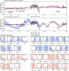 |
Fig. 4 KELT-7b atmospheric retrieval of the transmission observations assuming thermochemical equilibrium (top panel) and free-chemistry (middle panel). The solid curves with shaded areas show the median and 1σ span of the posterior model spectra for PYRAT BAY (blue) and PLATON (pink), displayed at a resolution of R = 150. The black circle markers with error bars show observations used to constrain the models. The diamond markers show the model spectra integrated over the observing bands. Bottom panels: Posterior distribution of the model parameters (same color coding as above). The labels on top of each posterior show the mean and 1σ uncertainties for each parameter posterior (denoted with a dashed line and shaded area, respectively). Some parameters have been omitted from this figure (see Table 5 for the full list of free parameters). |
5.5 Independent reduction of the HST/WFC3 transmission spectrum
To test whether any instrumental artifact could explain the poor fit of the transmission spectrum thermochemical-equilibrium retrievals in the near-infrared band, we independently reduced the two HST/WFC3 transits obtained for Hubble proposal 14767 (PI D. Sing), publicly available on MAST. We used the Intermediate MultiAccum (IMA) files and both scanning directions, and adopted the method described in Bruno et al. (2018). Each scanning direction was analyzed individually, resulting in two separate transit datasets. In particular, because of the brightness of the star, its two-dimensional spectral width in the detector scanning direction required an extraction window as large as 50 rows per nondestructive read. We did not observe any problematic features in the spectra (see Fig. B.1).
We retained the spectra in the 1.115–1.617 μm range and binned them using 6-pixel-wide bins to obtain the spectrophotometric transits. The full-range light curves were fitted with a least-squares minimization algorithm implementing the BATMAN transit model (Kreidberg 2015). We assumed a circular orbit and relied on the scaled semi-major axis and orbital inclination reported by Bieryla et al. (2015), while fitting for the transit depth and mid-transit time. The stellar parameters obtained by the same authors were used to compute quadratic LD coefficients using the EXOCTK package (Stevenson et al. 2018; Fowler et al. 2018; Bourque et al. 2021).
The transit model was multiplied by an exponential function to include the HST ramp, a second-degree polynomial to model stellar flux variations around the transits, and a scaling constant C, following standard practice (see, e.g., Stevenson et al. 2014a):
![Mathematical equation: $\[S(t)=C\left(1+r_0 \theta+r_1 \theta^2\right)\left(1-e^{r_2 \phi+r_3}+r_4 \phi\right).\]$](/articles/aa/full_html/2025/08/aa52560-24/aa52560-24-eq96.png) (4)
(4)
Here, θ is the planetary orbital phase, ϕ is the HST orbit phase (with an additional phase offset fixed at 0.15, determined through trial and error), and r0...4 are parameters to fit. Once the parameters for the systematic noise were determined, all but the scaling constant were fixed to their best-fit value, and EMCEE, version 3.1.6 (Foreman-Mackey et al. 2013), was used to sample the posterior distributions of C and the transit parameters. Setting 200 walkers and 2500 steps for the MCMC chains, and discarding the first 500 iterations as burn-in, was enough for each chain to be longer than 50 times its integrated autocorrelation time (Goodman & Weare 2010).
For all spectroscopic channels, the transit depth posterior distributions of the two transits were merged, and the final transmission spectrum was derived from the 16th, 50th, and 84th percentiles of the combined posterior distribution. Our output is compared to Pluriel et al. (2020)’s in Fig. 5, and confirms the transmission spectrum trend in the WFC3 band.
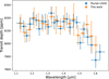 |
Fig. 5 Comparison of our independent extraction of the HST/WFC3 transmission spectrum and the one published by Pluriel et al. (2020). |
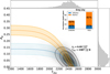 |
Fig. 6 Geometric albedo (Ag) as a function of the dayside brightness temperature for the estimated occultation depths in CHEOPS (blue) and TESS (red) passbands. The plot shows where the two curves intersect as well as the values of the two parameters. The black concentric curves depict 1,2, and 3σ distributions. The inset shows the reflection and emission contributions to the occultation depth for a gray-sky atmosphere. |
5.6 Albedo
A planetary brightness at occultation – that is, the brightness of the dayside hemisphere – can be expressed as the sum of the thermal emission (𝔼), which is a function of the brightness temperature (Tday), and reflection (ℝ) of the incident stellar light, which depends on the geometric albedo (Ag). The resultant brightness can be expressed as follows:
![Mathematical equation: $\[\frac{F_{\mathrm{p}}}{F_{\mathrm{s}}}=D_{\mathrm{occ}}=\mathbb{R}\left(A_{\mathrm{g}}\right)+\mathbb{E}\left(T_{\mathrm{day}}\right).\]$](/articles/aa/full_html/2025/08/aa52560-24/aa52560-24-eq97.png) (5)
(5)
Following the methodology described in Singh et al. (2024), we estimated the respective thermal emission and reflection/scattering contributions to the planetary brightness by assuming a gray-sky atmosphere, such that the geometric albedo and the brightness temperature are identical in the CHEOPS and TESS passbands. We obtain a very low geometric albedo of Ag = 0.05 ± 0.06 (<1σ). This corresponds to a brightness temperature of Tday = ![Mathematical equation: $\[2387_{-159}^{+123}\]$](/articles/aa/full_html/2025/08/aa52560-24/aa52560-24-eq98.png) K (see Fig. 6). These numbers indicate the 1σ upper limit of approximately 40% and 20% reflection contamination in the CHEOPS and TESS passbands, respectively. For comparison, the brightness temperature retrieved at 10−1 bar – where the atmosphere is most sensitive to optical wavelengths – is ~2500 K (see Fig. 3). Following this analytical approach, the brightness temperatures at Ag = 0 (no reflection) in TESS and CHEOPS are
K (see Fig. 6). These numbers indicate the 1σ upper limit of approximately 40% and 20% reflection contamination in the CHEOPS and TESS passbands, respectively. For comparison, the brightness temperature retrieved at 10−1 bar – where the atmosphere is most sensitive to optical wavelengths – is ~2500 K (see Fig. 3). Following this analytical approach, the brightness temperatures at Ag = 0 (no reflection) in TESS and CHEOPS are ![Mathematical equation: $\[2462_{-48}^{+45}\]$](/articles/aa/full_html/2025/08/aa52560-24/aa52560-24-eq99.png) K and
K and ![Mathematical equation: $\[2547_{-115}^{+90}\]$](/articles/aa/full_html/2025/08/aa52560-24/aa52560-24-eq100.png) K, respectively.
K, respectively.
Utilizing the eclipse (see Fig. 3) and transit spectra (see Fig. 4), we determined the planetary bolometric temperature. The resulting temperatures are approximately 2470 K and 2415 K, corresponding to the cases of equilibrium chemistry and free H− chemistry, respectively. Based on these temperature estimates, we derived upper limits for the Bond albedo (ϵ = 0, Cowan & Agol 2011): 0.0 ± 0.2 and 0.1 ± 0.2, respectively. In both cases, the Bond albedo remains consistent with zero within the given uncertainties. This indicates that the planet effectively absorbs nearly all incoming stellar irradiation to heat its dayside atmosphere.
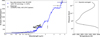 |
Fig. 7 Left panel: theoretically calculated dayside emission from the 3D GCM expeRT/MITgcm for KELT-7b including TiO and VO as well as high magnetic drag (blue line) compared to the observational data (black dots). The model data are binned down for better comparison with the observational data (blue dots, assuming the same uncertainty as the observational data). The 3D GCM model agrees within 1σ with the CHEOPS and TESS observations. Right panel: associated dayside averaged T-P profile. |
5.7 3D climate atmosphere modeling
As a sanity check for the retrieval models, we also simulated the dayside emission of the planet with the 3D general circulation model (GCM) expeRT/MITgcm (Schneider et al. 2022) as part of the ExoRad climate framework (Carone et al. 2020). We used the planetary parameters from Table 4 and the stellar parameters adopted from Tabernero et al. (2022b), described in Sect. 3, assuming solar metallicity and equilibrium chemistry for the planetary atmospheric composition. We further employed tabulated opacities for the following species: H2O from ExoMol (Tennyson et al. 2016, 2020), Na (Allard et al. 2019), K (Allard et al. 2019), CO2, CH4, NH3, CO, H2S, HCN, SiO, PH3, and FeH, as well as H− absorption and electron scattering, suitable for an ionized atmosphere (see, e.g., Helling et al. 2023). Appendix C contains a more detailed description of the model setup.
We find that to match the eclipse depths of KELT-7b in the CHEOPS and TESS bands simultaneously with those observed with Spitzer in the IRAC 1 and 2 bands, TiO and VO opacities and strong magnetic drag with τdrag = 104 s are needed. Ultrahot Jupiters similar to KELT-7b exhibit a strong horizontal gradient in ionization, as the dayside is thermally ionized, in contrast to the nightside (Helling et al. 2019, 2021). The degree of ionization also decreases with depth on the dayside, enabling magnetic coupling of the atmosphere to a global magnetic field (Rauscher & Menou 2013; Helling et al. 2023; Beltz et al. 2022). The inclusion of magnetic drag, which mimics the coupling of magnetic fields with the partially ionized flow, has become state-of-the-art for ultrahot Jupiters (see, e.g., Wardenier et al. 2023; Demangeon et al. 2024). The exact choice of τdrag is still debated, especially in the context of the uniform-drag assumption implemented here (Tan & Komacek 2019; Coulombe et al. 2023; Beltz et al. 2022). In this work, we used the smallest τdrag that effectively disrupts superrotation on the dayside in our GCM and shifts the onset of the dayside temperature inversion to deeper, higher-pressure layers compared to a simulation without drag, which retains efficient superrotation and horizontal wind transport (see Appendix C). Given the limited data, we only tested a few scenarios to constrain the range of the problem. One model without TiO and no drag, and two models with TiO – with and without strong drag – were explored. The latter two are shown in Appendix C. We find that, of these models, the one using strong drag with TiO best matched the data.
We further used an interface between expeRT/MITgcm and petitRADTRANS (Mollière et al. 2019) to generate dayside emission spectra. While the 3D climate model matches the TESS, CHEOPS, and Spitzer 4.5 μm observations well, it significantly underestimates the flux measured by HST/WFC3. At 3.6 μm, the predicted flux appears to be lower by about 2σ compared to Spitzer observations. The CFHT data point could not be reconciled with any tested atmospheric scenario; therefore, we discarded it from the analysis (see Fig. 7). Notably, the 3D climate model yields a temperature inversion that was not recovered by either retrieval model under the thermochemical-equilibrium assumption, only when adopting a free-chemistry parameterization. These models, however, use the HST/WFC3 data, which disagree with the predictions of the 3D GCM model. On the other hand, the choice of high magnetic drag in our 3D climate model yields inefficient horizontal heat distribution, which is consistent with the albedo results.
6 Discussion
Our attempt to understand the atmosphere of KELT-7b yields disparate results, depending on the approach and data used. Assuming the same geometric albedo and dayside temperature in the CHEOPS and TESS passbands, we find a low geometric albedo (Ag = 0.05 ± 0.06) and high dayside temperatures, consistent with inefficient horizontal heat distribution ϵ close to zero. Likewise, a 3D GCM simulation yields inefficient heat transfer, a TiO-induced temperature inversion, and a hot dayside temperature that fits the CHEOPS, TESS, and Spitzer data but not the HST/WFC3 data. The retrievals with PYRAT BAY and PLATON also confirm the low albedo result (see Sect. 5.3).
Two independent retrieval pipelines (PYRAT BAY and PLATON) yield consistent atmospheric results with each other, though they lead to different physical implications depending on the assumed modeling framework. Retrievals assuming thermochemical-equilibrium and free-chemistry abundances produce non-inverted and inverted thermal profiles, respectively. We note that the free-chemistry retrievals provide a better fit to the observations than the equilibrium-chemistry retrievals, even though the high brightness temperature of the occultations suggests that the atmosphere should be in thermochemical equilibrium. These inconclusive results may reflect limitations in both the physical models and data analysis methods. We also performed an independent reduction of the HST data using the method described in Bruno et al. (2018). This yields similar results to those published by Pluriel et al. (2020). Offsets between atmospheric spectra of the same planet obtained with different instruments are not uncommon (see, e.g., Murgas et al. 2020; Wilson et al. 2020; Yip et al. 2021; Edwards et al. 2024). Furthermore, some observations may be affected by stellar activity in this case, which could significantly hinder the correct interpretation of the brightness temperature (Tabernero et al. 2022b; Saba et al. 2025). Additionally, we note that stellar pulsations are reported for KELT-7b (Zhou et al. 2016; Stangret et al. 2022; Sicilia et al. 2025), which might additionally contaminate the planetary signal.
With a very simple calculation using Rs = 1.712 ± 0.037 R⊙, v sin Is = 71.4 ± 0.2 km s−1 (Tabernero et al. 2022b), and Is = 86 ± 25 deg (see Sect. 4.5) we can find a stellar rotational period of Prot,s = 1.22 ± 0.36 d, which is consistent with the maximum peak of the periodogram at 1.368 d (see middle panel of Fig. 1). This means that – given the planet’s host star is an F2V-type star with a convective envelope – in addition to the weak pulsations, mentioned earlier, the stellar variability (see Figs. A.4 and A.5; left panels) is very probably dominated by star spots, co-rotating with the star surface. Unocculted star spots can reduce the apparent stellar brightness, potentially deepening the measured planetary eclipse signal and leading to an overestimated planet’s dayside temperature (Zellem et al. 2017). The large inferred temperature variations of 400 K for KELT-7b in a narrow wavelength range suggest, however, a more complex scenario. In such a fast-rotating host star (Prot,s = 1.368 d), star spots may have rotated in and out of view during the HST/WFC3 observation. In addition, the oblateness of the rapidly rotating host star is expected to result in a stellar flux gradient from the equatorial (cooler) to the polar (hotter) regions according to the von Zeipel theorem (von Zeipel 1924a,b). The appearance and disappearance of star spots at different stellar latitudes during the observation may thus lead to nontrivial changes in the HST/WFC3 eclipse depth. However, a detailed assessment of stellar activity’s impact on the HST/WFC3 measurement lies beyond the scope of this work.
In this study, we accounted for the relatively high stellar variability of the fast-rotating host star KELT-7 when analyzing the TESS and CHEOPS data (see Sect. 4.2). Furthermore, our physically consistent atmospheric model fits the CHEOPS, TESS, and Spitzer data well, with the latter likely being least affected by stellar variability. We therefore consider our conclusions regarding the dayside temperature, low albedo, and inefficient heat transport – based on the combined CHEOPS and TESS data – to be robust. In any case, the example of the exoplanet KELT-7b underscores the need for a coherent modeling framework that incorporates physical noise sources, including stellar variability.
7 Conclusions
In this work, we analyzed the exoplanet KELT-7b with the main scientific goal of characterizing the atmosphere of the planet. Furthermore, we aimed to provide a precise measurement of KELT-7b’s albedo and to search for a possible distortion in its transit light curve caused by the rapid rotation of the host star. To fulfill these aims, we performed several photometric observations of KELT-7b secondary eclipses and transits using the CHEOPS space observatory. Moreover, we also used TESS photometric observations from seven sectors and literature data, which include published occultation and transit depths from HST/WFC3 and Spitzer/IRAC.
We first processed and jointly fitted the CHEOPS and TESS photometric data to detect the secondary eclipse of the planet in these passbands and to probe a potential asymmetry in the CHEOPS transit light curve. We were able to measure the occultation depths of KELT-7b with a ~3σ and ~8σ significance in the CHEOPS and TESS passbands, respectively. Our analysis yields the occultation depths of Docc,CHEOPS = 36 ± 11 ppm and Docc,TESS = 69 ± 9 ppm. We can conclude that the secondary eclipses of KELT-7b are relatively shallow in the CHEOPS and TESS passbands, which is characteristic of hot Jupiters (see, e.g., Singh et al. 2024; Pagano et al. 2024). In the optical wavelength range, the measured occultation depths are typically below 100 ppm.
Our most interesting results are related to the atmosphere modeling of KELT-7b. Based on the HST and Spitzer dataset, we performed occultation retrievals, and based on the CHEOPS, TESS, HST, and Spitzer dataset, transmission retrievals. We used two retrieval tools by applying the same set of assumptions to both frameworks as closely as permitted by their respective constraints. In all cases, we tested two alternatives, one following the free-chemistry parameterization and another assuming thermochemical equilibrium. We also tested a range of configurations to explore the dependence of the retrieval results on our assumptions. We can conclude that both retrieval codes produce consistent results when subjected to the same set of assumptions. When adopting a thermochemical-equilibrium atmospheric composition, the occultation retrievals return a non-inverted T-P profile with a composition characterized by C/O > 1, a super-solar metallicity, and a relatively weak H2O abundance. In contrast, when adopting a free-chemistry atmospheric parameterization, the occultation retrievals return an inverted T-P profile with – likely unphysically – high concentrations of TiO and VO. None of the additional tests resulted in qualitatively different retrieval results. The transmission retrievals in the thermochemical-equilibrium case support high metallicity, low C/O, and a cloud-free atmosphere; in the free-chemistry case, they detect H2O and an additional optical absorber.
Adopting a free-chemistry parameterization, Pluriel et al. (2020) and Changeat et al. (2022) find, via occultation retrievals on the HST/WFC3 and Spitzer data of KELT-7b, an inverted T-P profile, a nondetection of H2O, and a detection of H− absorption. Although these findings are in agreement with our results assuming free chemistry, and although the free-chemistry retrievals generally yield better fits to the observations, we can conclude that assuming free constant-with-altitude abundances risks adopting unphysical scenarios. The dayside atmosphere of ultrahot Jupiters similar to KELT-7b is hot enough, and the chemical reaction rates are fast enough to overcome the effect of disequilibrium chemistry. The equilibrium-chemistry approach was also previously applied by Changeat et al. (2022), finding via occultation retrievals solar to super-solar metallicities, C/O > 1, and a different thermal structure from the ones found by the free-chemistry runs. The equilibrium-chemistry retrieval on the transit spectrum does not lead to strong constraints in the transmission retrieval performed by Changeat et al. (2022), whereas only the free-chemistry retrieval returns H2O and H− absorption, in agreement with the results presented by Pluriel et al. (2020) and our findings. We can therefore conclude that the choice of a free-chemistry approach or a thermochemical-equilibrium chemistry is the main factor determining the retrieval results.
Given KELT-7b is an ultrahot Jupiter, although near the lower limit from the viewpoint of equilibrium temperature, the preferred non-inverted T-P profile does not support the predictions of Hubeny et al. (2003) and Fortney et al. (2008), similarly to the case of WASP-12b (Sing et al. 2013; Akinsanmi et al. 2024). However, as we mentioned in Sect. 1, and as we showed in Sect. 5.3, the identification of T-P inversion is a model-dependent process. The 3D GCM results support a TiO-induced temperature inversion, in tension with the results obtained via the thermochemical-equilibrium-based atmospheric retrievals. We can conclude that this discrepancy is because the occultation-retrieval models focus mainly on the HST data, while the 3D GCM model fits the CHEOPS, TESS, and Spitzer data, but underestimates the HST observations. Based on the retrieval results, we can also conclude that there might be a problem with the HST/WFC3 data in the case of this particular planet, which could be due to contamination of the data by stellar activity. As a consequence, the HST observations of KELT-7b suggest a high brightness temperature gradient that is difficult to reconcile with self-consistent atmospheric models. To support this argument, we independently reduced the HST/WFC3 transmission spectrum. Our output is in full agreement with Pluriel et al. (2020)’s, which means that with instrumental artifacts we cannot explain the poor thermochemical-equilibrium-retrievals fit of the HST/WFC3 transmission spectrum. We applied coherent stellar variability treatment on TESS and CHEOPS occultation measurements of KELT-7b, commensurate with the known stellar activity of the host star (Tabernero et al. 2022b). We conclude that HST/WFC3 observations of KELT-7b would also benefit from a coherent stellar variability treatment as proposed by Saba et al. (2025).
Although our attempt to understand the atmosphere of the ultrahot Jupiter KELT-7b with CHEOPS, TESS, and additional data ended with a discrepancy in the T-P profiles, depending on which approach and data are used, we report for the exoplanet KELT-7b a very low geometric albedo of Ag = 0.05 ± 0.06 in the CHEOPS and TESS passbands, which corresponds to a brightness temperature of Tday = ![Mathematical equation: $\[2387_{-159}^{+123}\]$](/articles/aa/full_html/2025/08/aa52560-24/aa52560-24-eq101.png) K. This supports previous observations that hot Jupiters have, in general, low geometric albedos. The very low geometric albedo is consistent with heat distribution ϵ being close to zero, and also consistent with the occultation retrieval results and with a 3D GCM simulation that includes magnetic drag (τdrag = 104 s). Utilizing the eclipse and transit spectra, we also derived upper limits for the Bond albedo, assuming ϵ = 0, finding values consistent with zero within the given uncertainties. We can conclude that the planet effectively absorbs nearly all incoming stellar irradiation to heat its dayside atmosphere.
K. This supports previous observations that hot Jupiters have, in general, low geometric albedos. The very low geometric albedo is consistent with heat distribution ϵ being close to zero, and also consistent with the occultation retrieval results and with a 3D GCM simulation that includes magnetic drag (τdrag = 104 s). Utilizing the eclipse and transit spectra, we also derived upper limits for the Bond albedo, assuming ϵ = 0, finding values consistent with zero within the given uncertainties. We can conclude that the planet effectively absorbs nearly all incoming stellar irradiation to heat its dayside atmosphere.
Given the rapid rotation of the host star, we also probed the precise CHEOPS transit light curves from the viewpoint of transit asymmetry. Unfortunately, several astrophysical effects in such systems remain poorly understood. The von Zeipel theorem (von Zeipel 1924a,b) is not strictly valid, and hence it needs further investigation. For example, Claret (2012) found significant deviations from the von Zeipel theorem at the upper layers of a distorted star in radiative equilibrium. Based on the CHEOPS photometry, we are unable to place any meaningful constraint on the sky-projected orbital obliquity. The obtained value is λ = 8 ± 105 deg. On the other hand, we find that the stellar inclination is Is = 86 ± 25 deg. We can conclude that additional CHEOPS observations would be necessary to put significant constraints on the sky-projected orbital obliquity via photometric methods.
Data availability
Photometry data of KELT-7 used in this work are available at the CDS via anonymous ftp to cdsarc.cds.unistra.fr (130.79.128.5) or via https://cdsarc.cds.unistra.fr/viz-bin/cat/J/A+A/700/A5.
Acknowledgements
We thank Quentin Changeat for the constructive comments and suggestions. CHEOPS is an ESA mission in partnership with Switzerland with important contributions to the payload and the ground segment from Austria, Belgium, France, Germany, Hungary, Italy, Portugal, Spain, Sweden, and the United Kingdom. The CHEOPS Consortium would like to gratefully acknowledge the support received by all the agencies, offices, universities, and industries involved. Their flexibility and willingness to explore new approaches were essential to the success of this mission. CHEOPS data analysed in this article will be made available in the CHEOPS mission archive (https://cheops.unige.ch/archive_browser/). This paper includes data collected with the TESS mission, obtained from the MAST data archive at the Space Telescope Science Institute (STScI). Funding for the TESS mission is provided by the NASA Explorer Program. STScI is operated by the Association of Universities for Research in Astronomy, Inc., under NASA contract NAS 5-26555. This research made use of the open source Python package exoctk, the Exoplanet Characterization Toolkit (Bourque et al. 2021). The authors thank M. Zhang for his help with the configuration of PLATON. ZG was supported by the VEGA grant of the Slovak Academy of Sciences No. 2/0031/22 and by the Slovak Research and Development Agency – the contract No. APVV-20-0148. P.E.C. is funded by the Austrian Science Fund (FWF) Erwin Schroedinger Fellowship, program J4595-N. LBo, GBr, VNa, IPa, GPi, RRa, GSc, VSi, and TZi acknowledge support from CHEOPS ASI-INAF agreement no. 2019-29-HH.0. TWi acknowledges support from the UKSA and the University of Warwick. ABr was supported by the SNSA. MNG is the ESA CHEOPS Project Scientist and Mission Representative, and as such also responsible for the Guest Observers (GO) Programme. MNG does not relay proprietary information between the GO and Guaranteed Time Observation (GTO) Programmes, and does not decide on the definition and target selection of the GTO Programme. LCa and CHe acknowledge financial support from the Österreichische Akademie der Wissenschaften and from the European Union H2020-MSCA-ITN-2019 under Grant Agreement no. 860470 (CHAMELEON). Calculations were performed using supercomputer resources provided by the Vienna Scientific Cluster (VSC). ML acknowledges the support of the Swiss National Science Foundation under grant number PCEFP2_194576. This work was supported by FCT – Fundação para a Ciência e a Tecnologia through national funds and by FEDER through COMPETE2020 through the research grants UIDB/04434/2020, UIDP/04434/2020, 2022.06962.PTDC. O.D.S.D. is supported in the form of a work contract (DL 57/2016/CP1364/CT0004) funded by national funds through FCT. YAl acknowledges support from the Swiss National Science Foundation (SNSF) under grant 200020_192038. We acknowledge financial support from the Agencia Estatal de Investigación of the Ministerio de Ciencia e Innovación MCIN/AEI/10.13039/501100011033 and the ERDF “A way of making Europe” through projects PID2019-107061GB-C61, PID2019-107061GB-C66, PID2021-125627OB-C31, PID2021-125627OB-C32, and PID2023-150468NB-I00, from the Centre of Excellence “Severo Ochoa” award to the Instituto de Astrofísica de Canarias (CEX2019-000920-S), from the Centre of Excellence “María de Maeztu” award to the Institut de Ciències de l’Espai (CEX2020-001058-M), and from the Generalitat de Catalunya/CERCA programme. C.B. acknowledges support from the Swiss Space Office through the ESA PRODEX program. This work has been carried out within the framework of the NCCR PlanetS supported by the Swiss National Science Foundation under grants 51NF40_182901 and 51NF40_205606. ACC acknowledges support from STFC consolidated grant number ST/V000861/1, and UKSA grant number ST/X002217/1. ACMC acknowledges support from the FCT, Portugal, through the CFisUC projects UIDB/04564/2020 and UIDP/04564/2020, with DOI identifiers 10.54499/UIDB/04564/2020 and 10.54499/UIDP/04564/2020, respectively. This project was supported by the CNES. B.-O.D. acknowledges support from the Swiss State Secretariat for Education, Research and Innovation (SERI) under contract number MB22.00046. A.C., A.D., B.E., K.G., and J.K. acknowledge their role as ESA-appointed CHEOPS Science Team Members. This project has received funding from the Swiss National Science Foundation for project 200021_200726. It has also been carried out within the framework of the National Centre of Competence in Research PlanetS supported by the Swiss National Science Foundation under grant 51NF40_205606. The authors acknowledge the financial support of the SNSF. MF and CMP gratefully acknowledge the support of the Swedish National Space Agency (DNR 65/19, 174/18). DG gratefully acknowledges financial support from the CRT foundation under Grant No. 2018.2323 “Gaseous or rocky? Unveiling the nature of small worlds”. M.G. is an F.R.S.-FNRS Senior Research Associate. CHe acknowledges the European Union H2020-MSCA-ITN-2019 under Grant Agreement no. 860470 (CHAMELEON), and the HPC facilities at the Vienna Science Cluster (VSC). KGI is the ESA CHEOPS Project Scientist and is responsible for the ESA CHEOPS Guest Observers Programme. She does not participate in, or contribute to, the definition of the Guaranteed Time Programme of the CHEOPS mission through which observations described in this paper have been taken, nor to any aspect of target selection for the programme. K.W.F.L. was supported by Deutsche Forschungsgemeinschaft grants RA714/14-1 within the DFG Schwerpunkt SPP 1992, Exploring the Diversity of Extrasolar Planets. This work was granted access to the HPC resources of MesoPSL financed by the Region Ile de France and the project Equip@Meso (reference ANR-10-EQPX-29-01) of the programme Investissements d’Avenir supervised by the Agence Nationale pour la Recherche. PM acknowledges support from STFC research grant number ST/R000638/1. This work was also partially supported by a grant from the Simons Foundation (PI Queloz, grant number 327127). NCSa acknowledges funding by the European Union (ERC, FIERCE, 101052347). Views and opinions expressed are however those of the author(s) only and do not necessarily reflect those of the European Union or the European Research Council. Neither the European Union nor the granting authority can be held responsible for them. A. S. acknowledges support from the Swiss Space Office through the ESA PRODEX program. S.G.S. acknowledges support from FCT through FCT contract nr. CEECIND/00826/2018 and POPH/FSE (EC). The Portuguese team thanks the Portuguese Space Agency for the provision of financial support in the framework of the PRODEX Programme of the European Space Agency (ESA) under contract number 4000142255. GyMSz acknowledges the support of the Hungarian National Research, Development and Innovation Office (NKFIH) grant K-125015, a PRODEX Experiment Agreement No. 4000137122, the Lendület LP2018-7/2021 grant of the Hungarian Academy of Science and the support of the city of Szombathely. V.V.G. is an F.R.S-FNRS Research Associate. JV acknowledges support from the Swiss National Science Foundation (SNSF) under grant PZ00P2_208945. EV acknowledges support from the ‘DISCOBOLO’ project funded by the Spanish Ministerio de Ciencia, Innovación y Universidades under grant PID2021-127289NB-I00. NAW acknowledges UKSA grant ST/R004838/1. TZi acknowledges NVIDIA Academic Hardware Grant Program for the use of the Titan V GPU card and the Italian MUR Departments of Excellence grant 2023-2027 “Quantum Frontiers”. This project has received funding from the HUN-REN Hungarian Research Network.
Appendix A Supplementary light curves
Here we present supplementary light curves related to the joint fit of the CHEOPS and TESS data for eclipse detection (see Sect. 4.4).
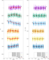 |
Fig. A.1 Phase-folded, and binned individual CHEOPS secondary eclipse observations of KELT-7b from visits 1 − 6, overplotted with the best-fitting CONAN3 model and arbitrarily shifted in flux for clarity. The left panel shows the nondetrended data overplotted with the full model, while the right panel shows the detrended data overplotted with the occultation model. |
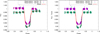 |
Fig. A.3 Phase-folded, individual CHEOPS transit observations of KELT-7b from visits 13 − 14, overplotted with the best-fitting CONAN3 model and arbitrarily shifted in flux for clarity. The left panel shows the nondetrended data overplotted with the full model, while the right panel shows the detrended data overplotted with the transit model. |
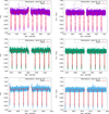 |
Fig. A.4 TESS observations of KELT-7b from Sectors 19, 43, and 44, overplotted with the best-fitting CONAN3 model. The left panels show the nondetrended data overplotted with the full model, while the right panels show the detrended data overplotted with the transit and occultation model. |
Appendix B Independent HST/WFC3 transit data reduction
Here we present diagnostic plots of the HST/WFC3 data reduction discussed in Sect. 5.5. Each plot, corresponding to one transit, shows all spectra of that visit divided by the median of the visit’s first ten spectra.
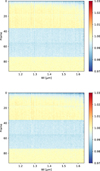 |
Fig. B.1 Normalized time sequence of the HST/WFC3 spectra corresponding to the two transits reduced as in Sect. 5.5. The y-axis represents increasing time with increasing frame number. |
Appendix C Detailed GCM set-up, chemistry and climate diagnostics
The GCM expeRT/MITgcm (Schneider et al. 2022) used in this work as part of the ExoRad climate framework (Carone et al. 2020) uses the MITgcm dynamical core that solves the hydrostatic primitive equations (see, e.g., Showman et al. 2009) in an Arakawa C-type cubed-sphere (Adcroft et al. 2004). The horizontal grid comprises 128 × 64 cells in longitude and latitude, respectively. The vertical grid consists of 47 cells in total: 41 logarithmically spaced cells between 10−5 bar and 100 bar, and six linearly spaced cells between 100 bar and 700 bar.
A fourth-order Shapiro filter is applied to the horizontal wind field, which suppresses small grid-scale noise. The damping timescale of the filter is set to τshap = 25 s, equal to the dynamical time step Δt = 25 s.7 The GCM is further stabilized against gravity wave reflection on top of the modeling domain with a sponge layer between 10−4 and 10−5. In this layer, the zonal horizontal velocity u is damped towards its longitudinally averaged mean ![Mathematical equation: $\[\bar{u}\]$](/articles/aa/full_html/2025/08/aa52560-24/aa52560-24-eq102.png) via the following relation:
via the following relation:
![Mathematical equation: $\[\frac{\mathrm{d} u}{\mathrm{~d} t}=-k(u-\bar{u}).\]$](/articles/aa/full_html/2025/08/aa52560-24/aa52560-24-eq103.png) (C.1)
(C.1)
Here, t is time and k is the strength of the Rayleigh prescription applied in the sponge layer, depending on pressure p as
![Mathematical equation: $\[k=k_{\text {top }} \cdot \max \left[0,1-\left(\frac{p}{p_{\text {sponge }}}\right)^2\right]^2.\]$](/articles/aa/full_html/2025/08/aa52560-24/aa52560-24-eq104.png) (C.2)
(C.2)
The control parameters psponge and ktop determine the position and strength of friction in the sponge layer. In this paper, the default values of ktop = 20 days−1 and psponge = 10−4 bar are used (Carone et al. 2020).
To stabilize the model against shear flow instabilities at the bottom boundary, basal drag is applied to the zonal wind velocity u and meridional wind velocity v in pressure layers deeper than 400 bar via:
![Mathematical equation: $\[\frac{\mathrm{d} u}{\mathrm{~d} t}=-k_{\mathrm{deep}} \cdot u,\]$](/articles/aa/full_html/2025/08/aa52560-24/aa52560-24-eq105.png) (C.3)
(C.3)
![Mathematical equation: $\[\frac{\mathrm{d} v}{\mathrm{~d} t}=-k_{\text {deep }} \cdot v,\]$](/articles/aa/full_html/2025/08/aa52560-24/aa52560-24-eq106.png) (C.4)
(C.4)
where the control parameter kdeep is defined as
![Mathematical equation: $\[k_{\mathrm{deep}}=k_{\mathrm{bottom}} \cdot \max \left[0, \frac{p-490 ~\mathrm{bar}}{700 ~\mathrm{bar}-490 ~\mathrm{bar}}\right]\]$](/articles/aa/full_html/2025/08/aa52560-24/aa52560-24-eq107.png) (C.5)
(C.5)
with kbottom = 1 day−1.
The model is started without wind flow and an initial analytical 1D temperature profile, following the formalism of Parmentier et al. (2015) with the host star’s parameters as listed in Sect. 3, a semi-major axis of 0.0442 AU, and an interior temperature of Tint = 663 K, following the fit of Thorngren et al. (2019). The model is run with the dynamical timestep of Δt = 25 s, where fluxes are recalculated every fourth dynamical timestep. The model is run for a 1000-day simulation time to ensure that the temperature structure does not evolve further in the modeling domain in the last 100 days. The final model output is derived by time averaging over the last 100 days of the whole simulation run. We note that there is some discrepancy in the host star parameters because some data were reduced based on the parameters from Pluriel et al. (2020). However, we note that the GCM here is used to provide a physical background to the possible climate state of this planet. A small change in the host star temperature will not strongly shift the climate states, for example, the need to include TiO/VO and magnetic drag to explain the overall flux. Furthermore, we note that we match CHEOPS, TESS, and Spitzer data sufficiently well to give us confidence that we capture the basic thermodynamics of the planetary atmosphere. Performance and stability tests for the sponge layer and basal drag are presented in Carone et al. (2020). A more detailed description of the radiative transfer implementation and performance tests can be found in Schneider et al. (2022).
In addition, a more detailed diagnostic of the climate state is useful to understand the impact of model choice on the day-side emission spectrum based on the GCM (see Fig. 7). Figure C.1 shows that for a climate model with TiO and magnetic drag, the dayside is heated up strongly between p = 10−2 − 10−3 bar (see also Fig. 7, right panel). Due to strong magnetic drag, superrotation (fast eastward wind jet along the equator) is effectively suppressed. Instead, direct radial flow from the day to the nightside is present for p < 10−2 bar. This climate state leads to a strong divergence in the horizontal wind flow field, which is closed by wind flow convergence in deeper layers (p > 1 bar). The choice of τdrag = 104 s has been shown in several GCM simulations for similar ultrahot Jupiters such as WASP-76b (Demangeon et al. 2024) and WASP-18b (Deline et al., in review) to consistently lead to a climate state with no superrotation, and consequently, no eastward hot spot shift, as also shown here. In particular, for WASP-18b it becomes apparent that τdrag = 104 s, which effectively prohibits the formation of superrotation, appears to yield dayside emission that agrees remarkably well even with the JWST data. In contrast, a climate model containing TiO and no magnetic drag shows that the dayside hot spot is partly shifted eastwards due to the presence of a superrotating jet (see Fig. C.3). Here, the regions of wind flow convergence are the Rossby gyres located at the morning terminator. Thus, with these two extreme choices in drag, we can explore two possible climate states or regimes that shape the dayside 3D temperature and chemistry that are measured with the eclipse spectra. Thus, a simulation with τdrag = 104 s represents a markedly different climate regime, dominated by radial wind flow rather than eastward jets. Such extreme scenarios can be used to meaningfully discuss efficient versus inefficient day-to-nightside heat transport. Higher τdrag (not explored here) typically leads to a climate with some remnant of superrotation, which would be an intermediate step, and here of limited usability.
Figures C.2 and C.4 show the dayside-averaged abundances and T-P profile for the GCM with and without drag, respectively. The model expeRT/MITgcm uses the equilibrium-chemistry package of petitRADTRANS (Mollière et al. 2019). Thus, we also use this package to derive the chemical abundances of species on the dayside of KELT-7b. It is evident that in the model with strong magnetic drag, the temperature inversion occurs at deeper pressures compared to the model with no magnetic drag. Furthermore, in both models, partial ionization of the atmosphere is evident in the upper atmosphere (p < 10−2 bar) as the abundances of H2 drop. Interestingly, the magnetic-drag model exhibits a temperature regime between 1 and 10 bar, where TiO and VO are less thermally stable, resulting in a local minimum for these two species. Because the region between 1 and 10 bar in the GCM with drag also represents the coldest part of the dayside atmosphere, the degree of ionization is particularly low there, resulting in a minimum of electron and atomic hydrogen abundances. It should be noted that in the model without drag, the coldest temperature regions lie comparatively higher at p ≈ 10−1 bar. Consequently, a local minimum in electron and atomic H abundances at the same pressure levels can be found. TiO and VO are, however, more thermally stable at these lower pressures. In fact, the TiO and VO abundances do not vary strongly on the dayside in the vertical direction in this drag-free simulation.
The comparison of temperatures and equilibrium chemistry in the GCMs with and without magnetic drag reveals that there is no direct causal connection between electron abundance minima and TiO and VO abundance minima. The question of whether and where TiO and VO may condense out of the atmosphere in hot Jupiters is, however, an ongoing research question (Roth et al. 2024; Beatty et al. 2017; Evans et al. 2016; Parmentier et al. 2013). In this work, the presence of TiO and VO may be favored due to the relatively high eclipse depths measured in the optical with CHEOPS, TESS, HST, and Spitzer.
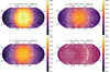 |
Fig. C.1 Horizontal slices in the GCM with TiO and strong magnetic drag of τdrag = 104 s across four representative pressure levels. Colors denote the local gas temperatures, white lines and arrows depict the horizontal wind flow, including regions of strong divergence/convergence at the substellar point (lat.: 0°, lon.: 0°). |
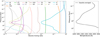 |
Fig. C.2 Left panel: Dayside averaged equilibrium gas-phase chemistry from the GCM with TiO and VO and with strong magnetic drag. Right panel: Dayside average T-P profile. |
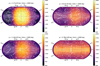 |
Fig. C.3 Horizontal slices in the GCM with TiO and with no magnetic drag across four representative pressure levels. Colors denote the local gas temperatures, white lines and arrows depict the horizontal wind flow. |
References
- Adcroft, A., Campin, J.-M., Hill, C., & Marshall, J. 2004, MWRv, 132, 2845 [Google Scholar]
- Akinsanmi, B., Barros, S. C. C., Lendl, M., et al. 2024, A&A, 685, A63 [NASA ADS] [CrossRef] [EDP Sciences] [Google Scholar]
- Allard, N. F., Spiegelman, F., Leininger, T., & Molliere, P. 2019, A&A, 628, A120 [NASA ADS] [CrossRef] [EDP Sciences] [Google Scholar]
- Angerhausen, D., DeLarme, E., & Morse, J. A. 2015, PASP, 127, 1113 [NASA ADS] [CrossRef] [Google Scholar]
- Arcangeli, J., Désert, J.-M., Line, M. R., et al. 2018, ApJ, 855, L30 [Google Scholar]
- Barman, T. S., Hauschildt, P. H., & Allard, F. 2005, ApJ, 632, 1132 [Google Scholar]
- Barnes, J. W. 2009, ApJ, 705, 683 [Google Scholar]
- Beatty, T. G., Madhusudhan, N., Tsiaras, A., et al. 2017, AJ, 154, 158 [NASA ADS] [CrossRef] [Google Scholar]
- Bell, T. J., & Cowan, N. B. 2018, ApJ, 857, L20 [Google Scholar]
- Bell, T. J., Welbanks, L., Schlawin, E., et al. 2023, Nature, 623, 709 [Google Scholar]
- Beltz, H., Rauscher, E., Kempton, E. M. R., et al. 2022, AJ, 164, 140 [NASA ADS] [CrossRef] [Google Scholar]
- Benz, W., Broeg, C., Fortier, A., et al. 2021, ExA, 51, 109 [Google Scholar]
- Bernath, P. F. 2020, JQSRT, 240, 106687 [NASA ADS] [CrossRef] [Google Scholar]
- Bieryla, A., Collins, K., Beatty, T. G., et al. 2015, AJ, 150, 12 [NASA ADS] [CrossRef] [Google Scholar]
- Bonfanti, A., Delrez, L., Hooton, M. J., et al. 2021, A&A, 646, A157 [EDP Sciences] [Google Scholar]
- Borucki, W. J., Koch, D., Basri, G., et al. 2010, Science, 327, 977 [Google Scholar]
- Borysow, A. 2002, A&A, 390, 779 [NASA ADS] [CrossRef] [EDP Sciences] [Google Scholar]
- Borysow, A., & Frommhold, L. 1989, ApJ, 341, 549 [NASA ADS] [CrossRef] [Google Scholar]
- Borysow, J., Frommhold, L., & Birnbaum, G. 1988, ApJ, 326, 509 [NASA ADS] [CrossRef] [Google Scholar]
- Borysow, A., Frommhold, L., & Moraldi, M. 1989, ApJ, 336, 495 [NASA ADS] [CrossRef] [Google Scholar]
- Borysow, A., Jorgensen, U. G., & Fu, Y. 2001, JQSRT, 68, 235 [NASA ADS] [CrossRef] [Google Scholar]
- Bourque, M., Espinoza, N., Filippazzo, J., et al. 2021, The Exoplanet Characterization Toolkit (ExoCTK) [Google Scholar]
- Brandeker, A., Heng, K., Lendl, M., et al. 2022, A&A, 659, L4 [NASA ADS] [CrossRef] [EDP Sciences] [Google Scholar]
- Bressan, A., Marigo, P., Girardi, L., et al. 2012, MNRAS, 427, 127 [NASA ADS] [CrossRef] [Google Scholar]
- Brown, T. M. 2001, ApJ, 553, 1006 [NASA ADS] [CrossRef] [Google Scholar]
- Bruno, G., Lewis, N. K., Stevenson, K. B., et al. 2018, AJ, 155, 55 [NASA ADS] [CrossRef] [Google Scholar]
- Buchner, J., Georgakakis, A., Nandra, K., et al. 2014, A&A, 564, A125 [NASA ADS] [CrossRef] [EDP Sciences] [Google Scholar]
- Burrows, A., Marley, M. S., & Sharp, C. M. 2000, ApJ, 531, 438 [NASA ADS] [CrossRef] [Google Scholar]
- Burrows, A., Hubeny, I., & Sudarsky, D. 2005, ApJ, 625, L135 [Google Scholar]
- Carone, L., Baeyens, R., Mollière, P., et al. 2020, MNRAS, 496, 3582 [NASA ADS] [CrossRef] [Google Scholar]
- Carter, J. A., & Winn, J. N. 2009, ApJ, 704, 51 [Google Scholar]
- Carter, A. L., May, E. M., Espinoza, N., et al. 2024, NatAs, 8, 1008 [Google Scholar]
- Changeat, Q., Edwards, B., Al-Refaie, A. F., et al. 2022, ApJS, 260, 3 [NASA ADS] [CrossRef] [Google Scholar]
- Charbonneau, D., Brown, T. M., Noyes, R. W., & Gilliland, R. L. 2002, ApJ, 568, 377 [Google Scholar]
- Charbonneau, D., Allen, L. E., Megeath, S. T., et al. 2005, ApJ, 626, 523 [Google Scholar]
- Claret, A. 2012, A&A, 538, A3 [NASA ADS] [CrossRef] [EDP Sciences] [Google Scholar]
- Coles, P. A., Yurchenko, S. N., & Tennyson, J. 2019, MNRAS, 490, 4638 [CrossRef] [Google Scholar]
- Coulombe, L.-P., Benneke, B., Challener, R., et al. 2023, Nature, 620, 292 [NASA ADS] [CrossRef] [Google Scholar]
- Cowan, N. B., & Agol, E. 2011, ApJ, 729, 54 [Google Scholar]
- Csizmadia, S. 2020, MNRAS, 496, 4442 [Google Scholar]
- Csizmadia, S., Smith, A. M. S., Kálmán, S., et al. 2023, A&A, 675, A106 [NASA ADS] [CrossRef] [EDP Sciences] [Google Scholar]
- Cubillos, P. E. 2017, ApJ, 850, 32 [CrossRef] [Google Scholar]
- Cubillos, P. E., & Blecic, J. 2021, MNRAS, 505, 2675 [NASA ADS] [CrossRef] [Google Scholar]
- Cubillos, P., Harrington, J., Loredo, T. J., et al. 2017, AJ, 153, 3 [Google Scholar]
- da Silva, L., Girardi, L., Pasquini, L., et al. 2006, A&A, 458, 609 [NASA ADS] [CrossRef] [EDP Sciences] [Google Scholar]
- Deline, A., Hooton, M. J., Lendl, M., et al. 2022, A&A, 659, A74 [NASA ADS] [CrossRef] [EDP Sciences] [Google Scholar]
- Demangeon, O. D. S., Cubillos, P. E., Singh, V., et al. 2024, A&A, 684, A27 [NASA ADS] [CrossRef] [EDP Sciences] [Google Scholar]
- Deming, D., Seager, S., Richardson, L. J., & Harrington, J. 2005, Nature, 434, 740 [Google Scholar]
- Deming, D., Wilkins, A., McCullough, P., et al. 2013, ApJ, 774, 95 [Google Scholar]
- Dyrek, A., Min, M., Decin, L., et al. 2024, Nature, 625, 51 [Google Scholar]
- Edwards, B., Changeat, Q., Baeyens, R., et al. 2020, AJ, 160, 8 [Google Scholar]
- Edwards, B., Tsiaras, A., Changeat, Q., & Yip, K. H. 2024, RASTI, 3, 415 [Google Scholar]
- Espinoza, N., & Jordán, A. 2015, MNRAS, 450, 1879 [Google Scholar]
- Esteves, L. J., De Mooij, E. J. W., & Jayawardhana, R. 2013, ApJ, 772, 51 [NASA ADS] [CrossRef] [Google Scholar]
- Esteves, L. J., De Mooij, E. J. W., & Jayawardhana, R. 2015, ApJ, 804, 150 [Google Scholar]
- Evans, T. M., Sing, D. K., Wakeford, H. R., et al. 2016, ApJ, 822, L4 [NASA ADS] [CrossRef] [Google Scholar]
- Evans, T. M., Sing, D. K., Kataria, T., et al. 2017, Nature, 548, 58 [NASA ADS] [CrossRef] [Google Scholar]
- Fazio, G. G., Hora, J. L., Allen, L. E., et al. 2004, ApJS, 154, 10 [Google Scholar]
- Feroz, F., & Hobson, M. P. 2008, MNRAS, 384, 449 [NASA ADS] [CrossRef] [Google Scholar]
- Feroz, F., Hobson, M. P., & Bridges, M. 2009, MNRAS, 398, 1601 [NASA ADS] [CrossRef] [Google Scholar]
- Feroz, F., Hobson, M. P., Cameron, E., & Pettitt, A. N. 2019, OJAp, 2, 10 [Google Scholar]
- Foreman-Mackey, D. 2018, RNAAS, 2, 31 [NASA ADS] [Google Scholar]
- Foreman-Mackey, D., Hogg, D. W., Lang, D., & Goodman, J. 2013, PASP, 125, 306 [Google Scholar]
- Foreman-Mackey, D., Agol, E., Ambikasaran, S., & Angus, R. 2017, AJ, 154, 220 [Google Scholar]
- Fortney, J. J. 2005, MNRAS, 364, 649 [Google Scholar]
- Fortney, J. J., Lodders, K., Marley, M. S., & Freedman, R. S. 2008, ApJ, 678, 1419 [CrossRef] [Google Scholar]
- Fortier, A., Simon, A. E., Broeg, C., et al. 2024, A&A, 687, A302 [NASA ADS] [CrossRef] [EDP Sciences] [Google Scholar]
- Fournier-Tondreau, M., Pan, Y., Morel, K., et al. 2025, MNRAS, 539, 422 [Google Scholar]
- Fowler, J., Stevenson, K. B., Lewis, N. K., et al. 2018, in American Astronomical Society Meeting Abstracts, 232, 111.03 [Google Scholar]
- Fu, G., Welbanks, L., Deming, D., et al. 2024, Nature, 632, 752 [Google Scholar]
- Garhart, E., Deming, D., Mandell, A., et al. 2020, AJ, 159, 137 [NASA ADS] [CrossRef] [Google Scholar]
- Gelman, A., & Rubin, D. B. 1992, StaSc, 7, 457 [Google Scholar]
- Goodman, J., & Weare, J. 2010, CAMCoS, 5, 65 [Google Scholar]
- Gressier, A., Espinoza, N., Allen, N. H., et al. 2024, ApJ, 975, L10 [NASA ADS] [CrossRef] [Google Scholar]
- Guillot, T. 2010, A&A, 520, A27 [NASA ADS] [CrossRef] [EDP Sciences] [Google Scholar]
- Hargreaves, R. J., Bernath, P. F., Bailey, J., & Dulick, M. 2015, ApJ, 813, 12 [Google Scholar]
- Harris, G. J., Tennyson, J., Kaminsky, B. M., Pavlenko, Y. V., & Jones, H. R. A. 2006, MNRAS, 367, 400 [Google Scholar]
- Harris, G. J., Larner, F. C., Tennyson, J., et al. 2008, MNRAS, 390, 143 [NASA ADS] [CrossRef] [Google Scholar]
- Haynes, K., Mandell, A. M., Madhusudhan, N., Deming, D., & Knutson, H. 2015, ApJ, 806, 146 [NASA ADS] [CrossRef] [Google Scholar]
- Helling, C., Iro, N., Corrales, L., et al. 2019, A&A, 631, A79 [NASA ADS] [CrossRef] [EDP Sciences] [Google Scholar]
- Helling, C., Worters, M., Samra, D., Molaverdikhani, K., & Iro, N. 2021, A&A, 648, A80 [NASA ADS] [CrossRef] [EDP Sciences] [Google Scholar]
- Helling, C., Samra, D., Lewis, D., et al. 2023, A&A, 671, A122 [NASA ADS] [CrossRef] [EDP Sciences] [Google Scholar]
- Heng, K., & Demory, B.-O. 2013, ApJ, 777, 100 [NASA ADS] [CrossRef] [Google Scholar]
- Heng, K., Menou, K., & Phillipps, P. J. 2011, MNRAS, 413, 2380 [NASA ADS] [CrossRef] [Google Scholar]
- Hooton, M. J., de Mooij, E. J. W., Watson, C. A., et al. 2019, MNRAS, 486, 2397 [NASA ADS] [CrossRef] [Google Scholar]
- Hooton, M. J., Hoyer, S., Kitzmann, D., et al. 2022, A&A, 658, A75 [NASA ADS] [CrossRef] [EDP Sciences] [Google Scholar]
- Hoyer, S., Guterman, P., Demangeon, O., et al. 2020, A&A, 635, A24 [NASA ADS] [CrossRef] [EDP Sciences] [Google Scholar]
- Hubeny, I., Burrows, A., & Sudarsky, D. 2003, ApJ, 594, 1011 [Google Scholar]
- Husser, T. O., Wende-von Berg, S., Dreizler, S., et al. 2013, A&A, 553, A6 [NASA ADS] [CrossRef] [EDP Sciences] [Google Scholar]
- Jenkins, J. M., Twicken, J. D., McCauliff, S., et al. 2016, SPIE Conf. Ser.,. 9913, 99133E [Google Scholar]
- John, T. L. 1988, A&A, 193, 189 [NASA ADS] [Google Scholar]
- Jones, K., Morris, B. M., Demory, B. O., et al. 2022, A&A, 666, A118 [NASA ADS] [CrossRef] [EDP Sciences] [Google Scholar]
- Jørgensen, U. G., Hammer, D., Borysow, A., & Falkesgaard, J. 2000, A&A, 361, 283 [Google Scholar]
- JWST Transiting Exoplanet Community Early Release Science Team (Ahrer, E.-M., et al.) 2023, Nature, 614, 649 [NASA ADS] [CrossRef] [Google Scholar]
- Kálmán, S., Bókon, A., Derekas, A., et al. 2022, A&A, 660, L2 [NASA ADS] [CrossRef] [EDP Sciences] [Google Scholar]
- Kesseli, A. Y., Snellen, I. A. G., Alonso-Floriano, F. J., Mollière, P., & Serindag, D. B. 2020, AJ, 160, 228 [NASA ADS] [CrossRef] [Google Scholar]
- Kreidberg, L. 2015, PASP, 127, 1161 [Google Scholar]
- Kopparapu, R. k., Kasting, J. F., & Zahnle, K. J. 2012, ApJ, 745, 77 [NASA ADS] [CrossRef] [Google Scholar]
- Kreidberg, L., Bean, J. L., Désert, J.-M., et al. 2014, ApJ, 793, L27 [Google Scholar]
- Kreidberg, L., Line, M. R., Parmentier, V., et al. 2018, AJ, 156, 17 [NASA ADS] [CrossRef] [Google Scholar]
- Krenn, A. F., Lendl, M., Patel, J. A., et al. 2023, A&A, 672, A24 [NASA ADS] [CrossRef] [EDP Sciences] [Google Scholar]
- Kurucz, R. L. 1970, SAO Special Report, 309 [Google Scholar]
- Kurucz, R. L. 1979, ApJS, 40, 1 [NASA ADS] [CrossRef] [Google Scholar]
- Lecavelier Des Etangs, A., Pont, F., Vidal-Madjar, A., & Sing, D. 2008, A&A, 481, L83 [NASA ADS] [CrossRef] [Google Scholar]
- Leckrone, D. S., Cheng, E. S., Feinberg, L. D., et al. 1998, in American Astronomical Society Meeting Abstracts, 192, 35.08 [Google Scholar]
- Lendl, M., Cubillos, P. E., Hagelberg, J., et al. 2017, A&A, 606, A18 [NASA ADS] [CrossRef] [EDP Sciences] [Google Scholar]
- Lendl, M., Bouchy, F., Gill, S., et al. 2020a, MNRAS, 492, 1761 [NASA ADS] [CrossRef] [Google Scholar]
- Lendl, M., Csizmadia, S., Deline, A., et al. 2020b, A&A, 643, A94 [EDP Sciences] [Google Scholar]
- Li, G., Gordon, I. E., Rothman, L. S., et al. 2015, ApJS, 216, 15 [NASA ADS] [CrossRef] [Google Scholar]
- Line, M. R., Stevenson, K. B., Bean, J., et al. 2016, AJ, 152, 203 [NASA ADS] [CrossRef] [Google Scholar]
- Lothringer, J. D., Barman, T., & Koskinen, T. 2018, ApJ, 866, 27 [NASA ADS] [CrossRef] [Google Scholar]
- Louie, D. R., Mullens, E., Alderson, L., et al. 2025, AJ, 169, 86 [Google Scholar]
- MacDonald, R. J., & Madhusudhan, N. 2017, ApJ, 850, L15 [NASA ADS] [CrossRef] [Google Scholar]
- Madhusudhan, N. 2012, ApJ, 758, 36 [NASA ADS] [CrossRef] [Google Scholar]
- Madhusudhan, N., & Seager, S. 2009, ApJ, 707, 24 [NASA ADS] [CrossRef] [Google Scholar]
- Madhusudhan, N., Knutson, H., Fortney, J. J., & Barman, T. 2014, in Protostars and Planets VI, eds. H. Beuther, R. S. Klessen, C. P. Dullemond, & T. Henning, 739 [Google Scholar]
- Madhusudhan, N., Agúndez, M., Moses, J. I., & Hu, Y. 2016, SSRv, 205, 285 [Google Scholar]
- Madhusudhan, N., Sarkar, S., Constantinou, S., et al. 2023, ApJ, 956, L13 [NASA ADS] [CrossRef] [Google Scholar]
- Mansfield, M., Bean, J. L., Line, M. R., et al. 2018, AJ, 156, 10 [NASA ADS] [CrossRef] [Google Scholar]
- Martioli, E., Colón, K. D., Angerhausen, D., et al. 2018, MNRAS, 474, 4264 [CrossRef] [Google Scholar]
- Mayo, A. W., Fortenbach, C. D., Louie, D. R., et al. 2025, AJ, 170, 50 [Google Scholar]
- McKemmish, L. K., Yurchenko, S. N., & Tennyson, J. 2016, MNRAS, 463, 771 [NASA ADS] [CrossRef] [Google Scholar]
- McKemmish, L. K., Masseron, T., Hoeijmakers, H. J., et al. 2019, MNRAS, 488, 2836 [Google Scholar]
- Mikal-Evans, T., Sing, D. K., Goyal, J. M., et al. 2019, MNRAS, 488, 2222 [Google Scholar]
- Mollière, P., Wardenier, J. P., van Boekel, R., et al. 2019, A&A, 627, A67 [Google Scholar]
- Moses, J. I. 2014, RSPTA, 372, 20130073 [Google Scholar]
- Murgas, F., Chen, G., Nortmann, L., Palle, E., & Nowak, G. 2020, A&A, 641, A158 [NASA ADS] [CrossRef] [EDP Sciences] [Google Scholar]
- Nikolov, N., Sing, D. K., Fortney, J. J., et al. 2018, Nature, 557, 526 [CrossRef] [Google Scholar]
- Pagano, I., Scandariato, G., Singh, V., et al. 2024, A&A, 682, A102 [NASA ADS] [CrossRef] [EDP Sciences] [Google Scholar]
- Parmentier, V., Showman, A. P., & Lian, Y. 2013, A&A, 558, A91 [NASA ADS] [CrossRef] [EDP Sciences] [Google Scholar]
- Parmentier, V., Guillot, T., Fortney, J. J., & Marley, M. S. 2015, A&A, 574, A35 [NASA ADS] [CrossRef] [EDP Sciences] [Google Scholar]
- Parmentier, V., Line, M. R., Bean, J. L., et al. 2018, A&A, 617, A110 [NASA ADS] [CrossRef] [EDP Sciences] [Google Scholar]
- Pino, L., Désert, J.-M., Brogi, M., et al. 2020, ApJ, 894, L27 [Google Scholar]
- Pluriel, W., Whiteford, N., Edwards, B., et al. 2020, AJ, 160, 112 [NASA ADS] [CrossRef] [Google Scholar]
- Polyansky, O. L., Kyuberis, A. A., Zobov, N. F., et al. 2018, MNRAS, 480, 2597 [NASA ADS] [CrossRef] [Google Scholar]
- Powell, D., Feinstein, A. D., Lee, E. K. H., et al. 2024, Nature, 626, 979 [NASA ADS] [CrossRef] [Google Scholar]
- Puget, P., Stadler, E., Doyon, R., et al. 2004, SPIE Conf. Ser., 5492, 978 [Google Scholar]
- Rauscher, E., & Menou, K. 2013, ApJ, 764, 103 [NASA ADS] [CrossRef] [Google Scholar]
- Redfield, S., Endl, M., Cochran, W. D., & Koesterke, L. 2008, ApJ, 673, L87 [Google Scholar]
- Ricker, G. R., Winn, J. N., Vanderspek, R., et al. 2014, SPIE Conf. Ser., 9143, 914320 [Google Scholar]
- Roth, A., Parmentier, V., & Hammond, M. 2024, MNRAS, 531, 1056 [CrossRef] [Google Scholar]
- Rothman, L. S., Gordon, I. E., Barber, R. J., et al. 2010, JQSRT, 111, 2139 [NASA ADS] [CrossRef] [Google Scholar]
- Russell, H. N. 1916, ApJ, 43, 173 [Google Scholar]
- Saba, A., Thompson, A., Yip, K. H., et al. 2025, ApJS, 276, 70 [Google Scholar]
- Santos, N. C., Cristo, E., Demangeon, O., et al. 2020, A&A, 644, A51 [NASA ADS] [CrossRef] [EDP Sciences] [Google Scholar]
- Scandariato, G., Singh, V., Kitzmann, D., et al. 2022, A&A, 668, A17 [NASA ADS] [CrossRef] [EDP Sciences] [Google Scholar]
- Schneider, A. D., Carone, L., Decin, L., et al. 2022, A&A, 664, A56 [NASA ADS] [CrossRef] [EDP Sciences] [Google Scholar]
- Seager, S. 2010, Exoplanet Atmospheres: Physical Processes (Princeton University Press) [Google Scholar]
- Seager, S., & Sasselov, D. D. 2000, ApJ, 537, 916 [Google Scholar]
- Seager, S., Richardson, L. J., Hansen, B. M. S., et al. 2005, ApJ, 632, 1122 [NASA ADS] [CrossRef] [Google Scholar]
- Sedaghati, E., Boffin, H. M. J., MacDonald, R. J., et al. 2017, Nature, 549, 238 [Google Scholar]
- Showman, A. P., Fortney, J. J., Lian, Y., et al. 2009, ApJ, 699, 564 [NASA ADS] [CrossRef] [Google Scholar]
- Shulyak, D., Lara, L. M., Rengel, M., & Nèmec, N. E. 2020, A&A, 639, A48 [NASA ADS] [CrossRef] [EDP Sciences] [Google Scholar]
- Sicilia, D., Malavolta, L., Scandariato, G., et al. 2025, A&A, 693, A316 [NASA ADS] [CrossRef] [EDP Sciences] [Google Scholar]
- Sing, D. K., Lecavelier des Etangs, A., Fortney, J. J., et al. 2013, MNRAS, 436, 2956 [NASA ADS] [CrossRef] [Google Scholar]
- Sing, D. K., Wakeford, H. R., Showman, A. P., et al. 2015, MNRAS, 446, 2428 [NASA ADS] [CrossRef] [Google Scholar]
- Singh, V., Scandariato, G., Smith, A. M. S., et al. 2024, A&A, 683, A1 [NASA ADS] [CrossRef] [EDP Sciences] [Google Scholar]
- Smith, J. C., Stumpe, M. C., Van Cleve, J. E., et al. 2012, PASP, 124, 1000 [Google Scholar]
- Snellen, I. A. G., Albrecht, S., de Mooij, E. J. W., & Le Poole, R. S. 2008, A&A, 487, 357 [NASA ADS] [CrossRef] [EDP Sciences] [Google Scholar]
- Snellen, I. A. G., de Kok, R. J., de Mooij, E. J. W., & Albrecht, S. 2010, Nature, 465, 1049 [Google Scholar]
- Spiegel, D. S., Silverio, K., & Burrows, A. 2009, ApJ, 699, 1487 [Google Scholar]
- Stangret, M., Casasayas-Barris, N., Pallé, E., et al. 2022, A&A, 662, A101 [NASA ADS] [CrossRef] [EDP Sciences] [Google Scholar]
- Stevenson, K. B., Bean, J. L., Fabrycky, D., & Kreidberg, L. 2014a, ApJ, 796, 32 [NASA ADS] [CrossRef] [Google Scholar]
- Stevenson, K. B., Désert, J.-M., Line, M. R., et al. 2014b, Science, 346, 838 [Google Scholar]
- Stevenson, K., Fowler, J., Lewis, N. K., et al. 2018, in American Astronomical Society Meeting Abstracts, 231, 148.14 [Google Scholar]
- Stumpe, M. C., Smith, J. C., Van Cleve, J. E., et al. 2012, PASP, 124, 985 [Google Scholar]
- Stumpe, M. C., Smith, J. C., Catanzarite, J. H., et al. 2014, PASP, 126, 100 [Google Scholar]
- Swain, M. R., Vasisht, G., & Tinetti, G. 2008, Nature, 452, 329 [NASA ADS] [CrossRef] [Google Scholar]
- Swain, M. R., Tinetti, G., Vasisht, G., et al. 2009, ApJ, 704, 1616 [Google Scholar]
- Szabó, G. M., Szabó, R., Benkő, J. M., et al. 2011, ApJ, 736, L4 [Google Scholar]
- Tabernero, H. M., Marfil, E., Montes, D., & González Hernández, J. I. 2022a, A&A, 657, A66 [NASA ADS] [CrossRef] [EDP Sciences] [Google Scholar]
- Tabernero, H. M., Zapatero Osorio, M. R., Allende Prieto, C., et al. 2022b, MNRAS, 515, 1247 [NASA ADS] [CrossRef] [Google Scholar]
- Tan, X., & Komacek, T. D. 2019, ApJ, 886, 26 [Google Scholar]
- Tennyson, J., Yurchenko, S. N., Al-Refaie, A. F., et al. 2016, JMoSp, 327, 73 [Google Scholar]
- Tennyson, J., Yurchenko, S. N., Al-Refaie, A. F., et al. 2020, JQSRT, 255, 107228 [NASA ADS] [CrossRef] [Google Scholar]
- Thorngren, D., Gao, P., & Fortney, J. J. 2019, ApJ, 884, L6 [Google Scholar]
- Tsai, S.-M., Lee, E. K. H., Powell, D., et al. 2023, Nature, 617, 483 [CrossRef] [Google Scholar]
- Venot, O., Drummond, B., Miguel, Y., et al. 2018, ExA, 46, 101 [Google Scholar]
- von Zeipel, H. 1924a, MNRAS, 84, 665 [NASA ADS] [CrossRef] [Google Scholar]
- von Zeipel, H. 1924b, MNRAS, 84, 684 [NASA ADS] [CrossRef] [Google Scholar]
- Wardenier, J. P., Parmentier, V., Line, M. R., & Lee, E. K. H. 2023, MNRAS, 525, 4942 [NASA ADS] [CrossRef] [Google Scholar]
- Werner, M. W., Roellig, T. L., Low, F. J., et al. 2004, ApJS, 154, 1 [NASA ADS] [CrossRef] [Google Scholar]
- Wilson, P. A., Sing, D. K., Nikolov, N., et al. 2015, MNRAS, 450, 192 [Google Scholar]
- Wilson, J., Gibson, N. P., Nikolov, N., et al. 2020, MNRAS, 497, 5155 [NASA ADS] [CrossRef] [Google Scholar]
- Wong, I., Shporer, A., Kitzmann, D., et al. 2020, AJ, 160, 88 [Google Scholar]
- Wong, I., Kitzmann, D., Shporer, A., et al. 2021, AJ, 162, 127 [NASA ADS] [CrossRef] [Google Scholar]
- Yip, K. H., Changeat, Q., Edwards, B., et al. 2021, AJ, 161, 4 [CrossRef] [Google Scholar]
- Yurchenko, S. N. 2015, JQSRT, 152, 28 [Google Scholar]
- Zellem, R. T., Swain, M. R., Roudier, G., et al. 2017, ApJ, 844, 27 [NASA ADS] [CrossRef] [Google Scholar]
- Zhang, M., Paragas, K., Bean, J. L., et al. 2025, AJ, 169, 38 [Google Scholar]
- Zhou, G., Latham, D. W., Bieryla, A., et al. 2016, MNRAS, 460, 3376 [NASA ADS] [CrossRef] [Google Scholar]
In general there is a four-way degeneracy in Is and λ deduced from gravity darkening, such that we are unable to distinguish between λ, − λ, 180° − λ, and 180° + λ (see Smith et al., in prep., for more details). Here, λ is so poorly constrained that we report only one of these solutions, and draw no conclusions from the result.
The damping timescale τshap corresponds to the dissipation time τν used in Heng et al. (2011) to compare horizontal dissipation in different dynamical cores.
All Tables
Priors and posterior parameter estimations (median and 68% credible intervals) for the atmospheric retrievals.
All Figures
|
Fig. 1 Periodograms of KELT-7 TESS PDCSAP observations. The blue dashed line represents the fitted orbital period of the planet. The red dashed line represents the median value of the prior imposed on the stellar rotational period. Left panel: periodogram of TESS Sector 59 raw data, which was used to determine the prior. Middle panel: periodogram of the residuals of TESS Sector 45 data after removal of the transits and occultations. Right panel: periodogram of the residuals of TESS Sector 45 data. |
| In the text | |
|
Fig. 2 Phase-folded, detrended, and binned CHEOPS (top panels) and TESS (bottom panels) transit (left panels) and occultation (right panels) light curves of KELT-7b, overplotted with the best-fitting CONAN3 model. Residuals are also shown. |
| In the text | |
|
Fig. 3 KELT-7b atmospheric retrieval of the infrared occultations. Top left panel: retrievals assuming thermochemical equilibrium with PYRAT BAY (blue) and PLATON (pink). The solid curves with shaded areas show the median and 1σ span of the posterior model spectra, displayed at a resolution of R = 150. The black circle markers with error bars show observations used to constrain the models (HST and Spitzer). The green square markers show the CHEOPS and TESS occultation depths (not used as retrieval constraints). The diamond markers show the model spectra integrated over the observing bands. The insets zoom in on the regions probed by the observations. Top right panel: retrieved T–P profiles for each retrieval code (median and 1σ span from the posterior distribution, same color coding as previous panel). The gray hatched area denotes the range of pressures probed by the observations. Middle panels: same as above, but for the free-chemistry retrievals. Bottom panels: posterior distribution of the atmospheric composition parameters (same color coding as above). The labels on top of each posterior show the mean and 1σ uncertainties for each parameter posterior (denoted with a dashed line and shaded area, respectively). Some parameters have been omitted from this figure (see Table 5 for the full list of free parameters). |
| In the text | |
|
Fig. 4 KELT-7b atmospheric retrieval of the transmission observations assuming thermochemical equilibrium (top panel) and free-chemistry (middle panel). The solid curves with shaded areas show the median and 1σ span of the posterior model spectra for PYRAT BAY (blue) and PLATON (pink), displayed at a resolution of R = 150. The black circle markers with error bars show observations used to constrain the models. The diamond markers show the model spectra integrated over the observing bands. Bottom panels: Posterior distribution of the model parameters (same color coding as above). The labels on top of each posterior show the mean and 1σ uncertainties for each parameter posterior (denoted with a dashed line and shaded area, respectively). Some parameters have been omitted from this figure (see Table 5 for the full list of free parameters). |
| In the text | |
|
Fig. 5 Comparison of our independent extraction of the HST/WFC3 transmission spectrum and the one published by Pluriel et al. (2020). |
| In the text | |
|
Fig. 6 Geometric albedo (Ag) as a function of the dayside brightness temperature for the estimated occultation depths in CHEOPS (blue) and TESS (red) passbands. The plot shows where the two curves intersect as well as the values of the two parameters. The black concentric curves depict 1,2, and 3σ distributions. The inset shows the reflection and emission contributions to the occultation depth for a gray-sky atmosphere. |
| In the text | |
|
Fig. 7 Left panel: theoretically calculated dayside emission from the 3D GCM expeRT/MITgcm for KELT-7b including TiO and VO as well as high magnetic drag (blue line) compared to the observational data (black dots). The model data are binned down for better comparison with the observational data (blue dots, assuming the same uncertainty as the observational data). The 3D GCM model agrees within 1σ with the CHEOPS and TESS observations. Right panel: associated dayside averaged T-P profile. |
| In the text | |
|
Fig. A.1 Phase-folded, and binned individual CHEOPS secondary eclipse observations of KELT-7b from visits 1 − 6, overplotted with the best-fitting CONAN3 model and arbitrarily shifted in flux for clarity. The left panel shows the nondetrended data overplotted with the full model, while the right panel shows the detrended data overplotted with the occultation model. |
| In the text | |
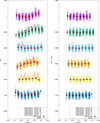 |
Fig. A.2 As in Fig. A.1, but for CHEOPS visits 7 − 12. |
| In the text | |
|
Fig. A.3 Phase-folded, individual CHEOPS transit observations of KELT-7b from visits 13 − 14, overplotted with the best-fitting CONAN3 model and arbitrarily shifted in flux for clarity. The left panel shows the nondetrended data overplotted with the full model, while the right panel shows the detrended data overplotted with the transit model. |
| In the text | |
|
Fig. A.4 TESS observations of KELT-7b from Sectors 19, 43, and 44, overplotted with the best-fitting CONAN3 model. The left panels show the nondetrended data overplotted with the full model, while the right panels show the detrended data overplotted with the transit and occultation model. |
| In the text | |
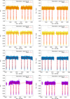 |
Fig. A.5 As in Fig. A.4, but for the TESS Sectors 45, 59, 71, and 73. |
| In the text | |
|
Fig. B.1 Normalized time sequence of the HST/WFC3 spectra corresponding to the two transits reduced as in Sect. 5.5. The y-axis represents increasing time with increasing frame number. |
| In the text | |
|
Fig. C.1 Horizontal slices in the GCM with TiO and strong magnetic drag of τdrag = 104 s across four representative pressure levels. Colors denote the local gas temperatures, white lines and arrows depict the horizontal wind flow, including regions of strong divergence/convergence at the substellar point (lat.: 0°, lon.: 0°). |
| In the text | |
|
Fig. C.2 Left panel: Dayside averaged equilibrium gas-phase chemistry from the GCM with TiO and VO and with strong magnetic drag. Right panel: Dayside average T-P profile. |
| In the text | |
|
Fig. C.3 Horizontal slices in the GCM with TiO and with no magnetic drag across four representative pressure levels. Colors denote the local gas temperatures, white lines and arrows depict the horizontal wind flow. |
| In the text | |
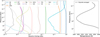 |
Fig. C.4 As in Fig C.2, but with no magnetic drag. |
| In the text | |
Current usage metrics show cumulative count of Article Views (full-text article views including HTML views, PDF and ePub downloads, according to the available data) and Abstracts Views on Vision4Press platform.
Data correspond to usage on the plateform after 2015. The current usage metrics is available 48-96 hours after online publication and is updated daily on week days.
Initial download of the metrics may take a while.