© The Authors 2025

1 Introduction

Protoplanetary discs are the cradles of planets, and their evolution and dispersal strongly affect the process of planet formation; therefore, studying the mechanism that drives accretion in discs is fundamental to understanding the formation of planetary systems. Traditionally, accretion is explained by the redistribution of angular momentum throughout the disc (Lynden-Bell & Pringle 1974; Pringle 1981). The transport of angular momentum is triggered by the presence of turbulence, parametrised by the α prescription of Shakura & Sunyaev (1973). In this scenario, disc dispersal is explained by photoevaporative winds launched from the disc surface when heated by stellar energetic radiation (Hollenbach et al. 1994; Alexander et al. 2014; Ercolano & Pascucci 2017). Numerical simulations have shown that X-ray and far-ultraviolet (FUV) photons coming from the central star can trigger a thermal wind, whose emission peaks at 1–10 au (Gorti & Hollenbach 2009; Owen et al. 2010; Nakatani et al. 2018; Picogna et al. 2019; Sellek et al. 2024). Moreover, models that combine viscous accretion and dispersal due to internal photoevaporation (Clarke et al. 2001; Alexander et al. 2006; Owen et al. 2012) can reproduce the observed disc properties and disc dispersal time (Hernández et al. 2007; Fedele et al. 2010). However, recent observational constraints pointing to low turbulence in discs (see Rosotti 2023 for a review) represent a challenge for the viscous paradigm. The best alternative to the classic viscous framework is the magnetohydrodynamical (MHD) winds model, proposed by Blandford & Payne (1982) and refined by recent studies (see Lesur 2021 for a review). This theory suggests that angular momentum and mass are both removed by MHD winds.

The advent of a new generation of instruments, such as the Atacama Large Millimeter and submillimeter Array (ALMA) and the Very Large Telescope (VLT), has allowed numerous surveys of different star-forming regions to be performed (see Manara et al. 2023 for a review). These surveys have measured various macroscopic disc quantities, such as the dust mass (e.g. Miotello et al. 2016; Barenfeld et al. 2016; Ansdell et al. 2016, 2017; Bergin & Williams 2017; Cazzoletti et al. 2019; Testi et al. 2022), the mass accretion rate (e.g. Alcalá et al. 2014, 2017; Manara et al. 2017; Almendros-Abad et al. 2024), and the disc radius, measured using both dust (e.g. Tazzari et al. 2017; Andrews et al. 2018a; Hendler et al. 2020; Sanchis et al. 2020) and gas (e.g. Ansdell et al. 2018; Najita & Bergin 2018; Sanchis et al. 2020). Although the conversion presents multiple challenges (see Miotello et al. 2023 for a review), the millimetric flux, which traces dust mass, is often used as a proxy to measure disc gas mass.

The statistical relevance of these samples represents a unique opportunity to test our evolutionary models with the tool of population synthesis. However, neither of the two frameworks has been ruled out by the observations yet. Indeed, distinguishing the signatures of the two models in the observations has proven to be challenging. For instance, viscous models predict ‘viscous spreading’, the increase in the radius of gas discs due to the transport of angular momentum. However, the relationship between the observed gas radius and the expanding disc radius is not trivial (Toci et al. 2023). Since MHD wind simulations do not show this feature (e.g. Zagaria et al. 2022, who modelled the effect of MHD winds on dust discs), detecting an increasing radial size of the discs would be a signature of viscous evolution. However, to detect it, we would need a higher sensitivity and a larger sample size (Trapman et al. 2020). Moreover, detecting it using dust as a proxy remains complicated, mainly due to the presence of radial drift and substructures (Rosotti et al. 2019; Toci et al. 2021; Delussu et al. 2024).

Lodato et al. (2017) showed that the purely viscous model inherently reproduces the observed accretion rate ($\dot{M}$) – disc mass (M) correlation (see also Mulders et al. 2017), while Somigliana et al. (2022) extensively studied how a correlation between the initial disc parameters and the stellar mass M_⋆ can affect the evolution of the slopes. Somigliana et al. (2020) introduced internal photoevaporation to the population synthesis model of Lodato et al. (2017) and showed that the removal of light discs causes older populations to appear more massive. This feature had been noted in earlier models as well (e.g., Alexander & Armitage 2009). On the MHD side, Tabone et al. (2022b) showed that the properties of observed populations and the observed disc fraction can also be reproduced assuming a purely wind-driven evolution. In addition, Zallio et al. (2024) managed to reproduce the observed $\dot{M}-M$ correlation with the MHD wind model, assuming a power-law correlation between the initial mass and the accretion timescale.

Various population synthesis models have attempted to develop a method to disentangle the two models in observations. Somigliana et al. (2024) illustrated how MHD evolution causes a different evolution of the slopes of the M–M_⋆ and $\dot{M}-M_{\star }$ correlations with respect to the viscous-photoevaporative scenario. However, they emphasised that the current sample size does not allow us to distinguish between the two evolutionary models. A similar argument is made by Alexander et al. (2023), who state that a larger sample size, with N > 300, would enable us to distinguish the two models from the $\dot{M}$ distribution. Somigliana et al. (2023) investigated the spread of the $\dot{M}/M$ ratio as a proxy to disentangle the two models from the observations. They find a better agreement with the MHD wind model, although the observational spread does not allow us to rule out the viscous scenario. The picture is further complicated by the presence of external photoevaporation (Coleman et al. 2024), whose effect on disc masses and radii is not negligible even for moderately irradiated environments (Anania et al. 2024).

All of these endeavours highlight that measuring disc gas masses is crucial to understanding disc evolution from observed populations. For this purpose, the new large programme AGEPRO (Zhang et al. in prep.) have measured disc masses for three star-forming regions of different ages, using CO and N₂H⁺ as a proxy (Trapman et al. 2022). Tabone et al. (2025) attempted to reproduce the observed population with both the MHD wind model and the viscous model and find that the latter fails to simultaneously reproduce both masses and accretion rates. This result strengthens the support for the MHD wind model. Data from the DECO (Cleeves et al., in prep.) large programme will enhance the current sample size and allow us to verify this result and probe disc evolution. Hence, it is essential to identify the signatures of evolutionary models in disc populations and develop new proxies to distinguish them in observations.

In this study, we explored the evolution of the mass distribution of disc populations when dispersal is taken into consideration–a topic that has not been examined in the literature before. In particular, we investigated its behaviour under the assumptions of viscous evolution and dispersal driven by internal photoevaporation. We find that the evolution of the median mass is a signature of this model, and we propose it as a new proxy to distinguish between the viscous-photoevaporative framework and the MHD wind model in observed populations. We also introduce a new criterion to predict a disc’s lifetime based on its initial conditions. In Sect. 2 we present our analytical derivations, while in Sect. 3 we support them with numerical simulations. In Sect. 4, we discuss the implications of our results and compare them with different evolutionary pathways.

2 Analytical model

2.1 Overview: The viscous-photoevaporative model

In this section, we provide a brief overview of the viscous model coupled with dispersal due to internal photoevaporation. Accretion is explained by the radial transport of angular momentum, due to the presence of turbulence inside the disc. The gas surface density evolves according to the classic viscous evolution equation $$\frac{\partial \text{Σ}}{\partial t}=\frac{3}{R}\frac{\partial }{\partial R}\left(R^{1/2}\frac{\partial }{\partial R}\left(\alpha c_{\text{s}}H\text{Σ}{R}^{1/2}\right)\right)-{{\displaystyle \dot{\sum }}}_{\text{w}}(R),$$(1)

where R is the cylindrical radius and ${{\displaystyle \dot{\sum }}}_{\text{w}}$ the photoevaporative wind mass-loss rate per unit area. The parameterization of viscosity ν follows the Shakura & Sunyaev (1973) prescription ν = αc_sH, where c_s is the speed of sound, H the scale height of the disc, and α a dimensionless parameter that quantifies turbulence, typically assumed constant throughout the disc. In the purely viscous scenario ${{\displaystyle \dot{\sum }}}_{\text{w}}=0$ at all radii and Eq. (1) admits an analytical “self-similar” solution (Lynden-Bell & Pringle 1974), $${\text{Σ}}_{\text{SS}}(R,t)=\frac{M_0}{2\pi R{R}_0}{\left(1+\frac{t}{t_v}\right)}^{-3/2}\exp \left(-\frac{R}{R_0\left(1+t/t_v\right)}\right),$$(2)

where M₀ is the initial disc mass, R₀ is the initial truncation radius, and t_ν is the viscous timescale defined as t_ν = R₀²/3ν_c, where ν_c = ν(R = R₀). Equation (2) is valid under the assumption that viscosity scales as a power law as a function of radius, $$v=v_0{\left(R/R_0\right)}^{\gamma },$$(3)

where γ = 1 according to the relation T ∝ R^−1/2 (Hartmann et al. 1998), although solutions for different values of 0 < γ < 2 also exist. We make this assumption throughout the paper. The total disc mass, M, and the mass accretion rate onto the star, $\dot{M}$, evolve with time as $$M(t)=M_0{\left(1+\frac{t}{t_v}\right)}^{-1/2},$$(4) $$\dot{M}(t)=-\frac{\text{d}M}{\text{d}t}=\frac{M_0}{2t_v}{\left(1+\frac{t}{t_v}\right)}^{-3/2}.$$(5)

Equations (4) and (5) highlight that both the disc mass and the accretion rate onto the star decrease with time due to viscous accretion.

Internal photoevaporation introduces a mass-loss term ${{\displaystyle \dot{\sum }}}_{\text{w}}(R)$ that can be computed with hydro-dynamic simulations (Font et al. 2004; Alexander et al. 2006; Owen et al. 2012; Picogna et al. 2019), and it is often assumed to be solely dependent on R and constant with time. Moreover, for X-ray-driven photoevaporation, the radial profile of ${{\displaystyle \dot{\sum }}}_{\text{w}}(R)$ does not depend on the structure of the disc, as discussed in the literature (Owen et al. 2010, 2012). The total wind mass-loss rate ${\dot{M}}_{\text{w}}$ is obtained by integrating ${{\displaystyle \dot{\sum }}}_{\text{w}}(R)$ along the radial component. For simplicity, in this study, we considered only the Owen et al. (2012) ${{\displaystyle \dot{\sum }}}_{\text{w}}$ numerical profile. Numerical solutions of Eq. (1) show that winds carve a cavity in the disc at around 5 au, corresponding to the peak of the mass-loss rate profile (Picogna et al. 2021). Figure 1 shows this feature for a disc numerically evolved according to Eq. (1) using the code Diskpop (Somigliana et al. 2024). After the opening of the gap, the inner disc rapidly accretes onto the star, with a reduced viscous timescale (Clarke et al. 2001),

$$t_{v,\text{in}}=t_v\left(\frac{R_{\text{gap}}}{R_0}\right),$$(6)

where R_gap is the radial location of the gap, and R_gap ≪ R₀ leads to t_ν,in ≪ t_ν. The drainage of the inner disc results in a steep decrease in the accretion rate, whereas the disc mass remains relatively constant (see Fig. 2), due to the difficulty in dispersing the outer disc. The so-called ‘relic disc’ problem is a well-known challenge of models that account only for internal photoevaporation as a source of disc dispersal without considering the direct irradiation of the disc after the gap opening (Alexander et al. 2006; Owen & Kollmeier 2019; Robinson et al. 2025). Figure 2 shows the evolution of the mass and accretion rate over time for the same disc as in Fig. 1. Throughout this paper, we refer to dispersal time as the moment when either the disc mass or the accretion rate drops below the respective observational threshold (defined in Sect. 3), marking the object’s transition to Class III.

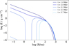Fig. 1 Evolution of the surface density of a disc over time, obtained by integrating Eq. (1) using Diskpop. This disc has M0 = 1.5 · 10−2 M⊙, R0 = 32.8 au, α = 10−3, and ${\dot{M}}_{\text{w}}=2.5\cdot {10}^{-9}{\text{M}}_{\odot }{\text{yr}}^{-1}$. After the opening of the gap, the inner disc is dispersed on a short timescale.

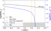Fig. 2 Evolution of the accretion rate (blue) and mass (black) of a disc over time. The vertical yellow line indicates the instant when the gap opens, which triggers a steep decrease in $\dot{M}$. The red line marks the transition between accreting and non-accreting phases. The grey region corresponds to values of disc mass and accretion rate below the respective observational threshold.

2.2 The disc lifetime: State of the art

The fast dispersal of the inner disc results in an intrinsic twotimescale nature of the viscous-photoevaporative model, namely the ‘ultraviolet switch’, introduced by Clarke et al. (2001). The first timescale corresponds to a slow viscous evolution, while the second one corresponds to a rapid clearance of the inner disc. Due to the two mechanisms of gas depletion, the evolution of the disc mass can be described by the following relation until the gap opening: $$\frac{\text{d}M(t)}{\text{d}t}\sim -\dot{M}(t)-{\dot{M}}_{\text{w}},$$(7)

where the accretion rate $\dot{M}(t)$ is a decreasing function of time (see Eq. (5)), while ${\dot{M}}_{\text{w}}$ remains constant. Assuming ${\dot{M}}_0\gg {\dot{M}}_{\text{w}}$, where ${\dot{M}}_0\equiv \dot{M}(0)$, photoevaporation is negligible during the initial phase of the disc evolution, and Eqs. (4) and (5) adequately describe the evolution of the disc’s macroscopic properties. However, as soon as $\dot{M}\left(t_{\text{w}}\right)={\dot{M}}_{\text{w}}$, the effect of winds becomes relevant. The time t_w, introduced by Clarke et al. (2001), marks the transition between the accretion-dominated regime and the photoevaporation-dominated regime. As a consequence, due to the rapid photoevaporative removal of the inner disc, t_w provides an estimate of the disc’s lifetime (Clarke et al. 2001; Somigliana et al. 2020; Picogna et al. 2021). The definition of t_w implies $$t_{\text{w}}=\frac{M_0}{2{\dot{M}}_0}{\left(\frac{{\dot{M}}_0}{{\dot{M}}_{\text{w}}}\right)}^{\frac{2}{3}}=t_v{\left(\frac{{\dot{M}}_0}{{\dot{M}}_{\text{w}}}\right)}^{\frac{2}{3}}\gg t_v$$(8)

in the t_ν ≪ t_w limit.

2.3 The disc lifetime: A new criterion

Equation (8) identifies the dispersal time as the moment when photoevaporation becomes the dominant driver of mass-loss on a global scale, a condition we refer to in this work as the ‘global criterion’. However, we can easily see that this criterion is not generally applicable. For example, if ${\dot{M}}_0<{\dot{M}}_{\text{w}}$, a scenario that cannot be excluded a priori, the criterion would predict a vanishingly small lifetime. This is because Eq. (8) does not take into account the finite time required for photoevaporation to deplete the surface density and open a gap, which, as illustrated by Fig. 2, marks the event that triggers the rapid dispersal of the inner disc. To derive this timescale, we need to make use of local quantities, such as the surface density, Σ, and the local mass-loss rate, ${{\displaystyle \dot{\sum }}}_w$. Therefore, we introduce a ‘local criterion’ that estimates the instant at which photoevaporative winds become locally relevant enough to cause the opening of a gap and the subsequent dispersal of the inner disc.

We can write the evolution of Σ(R, t) as a sum of a viscous term and a photoevaporative term: $$\text{Σ}(R,t)\sim {\text{Σ}}_{SS}(R,t)-{\dot{\Sigma }}_{\text{w}}(R)t,$$(9)

where Σ_SS(R, t) is given by Eq. (2). We stress that Eq. (9) is not a solution of Eq. (1), but rather an approximation. We define the local dispersal timescale, t_loc, as $$t_{\text{loc}}=\frac{{\text{Σ}}_{\text{SS}}\left(R_{\text{gap}},t_{\text{loc}}\right)}{{\dot{\Sigma }}_{\text{w}}\left(R_{\text{gap}}\right)}.$$(10)

This is the time at which Eq. (9) vanishes at R = R_gap, which corresponds to the minimum of $\text{Σ}(R)/{\dot{\Sigma }}_{\text{w}}(R)$. By considering the ${{\displaystyle \dot{\sum }}}_{\text{w}}(R)$ profile obtained by Owen et al. (2012), we find the local criterion of disc dispersal, $$\begin{array}{c}{t}_{\text{loc}}\sim 4.4\text{Myr}{\left(\frac{M_0}{{10}^{-2}\text{M}\odot }\right)}^{3/5}{\left(\frac{M_{\star }}{{\text{M}}_{\odot }}\right)}^{3/5}{\left(\frac{{\dot{M}}_0}{{10}^{-8}{\text{M}}_{\odot }y{r}^{-1}}\right)}^{-1/5}\\ \times {\left(\frac{{\dot{M}}_{\text{w}}}{{10}^{-9}{\text{M}}_{\odot }y{r}^{-1}}\right)}^{-2/5}{\left(\frac{\alpha }{{10}^{-3}}\right)}^{-2/5},\end{array}$$(11)

where $$R_{\text{gap}}=3.6\text{\hspace{0.17em}au}\left(\frac{M_{\star }}{{\text{M}}_{\odot }}\right),$$(12)

and $$\dot{\Sigma }\left(R_{\text{gap}}\right)=2.8\cdot {10}^{-11}{\text{M}}_{\odot }{\text{yr}}^{-1}{\text{au}}^{-2}\frac{1}{2\pi }{\left(\frac{M_{\star }}{{\text{M}}_{\odot }}\right)}^{-2}\left(\frac{{\dot{M}}_{\text{w}}}{{10}^{-9}{\text{M}}_{\odot }{\text{yr}}^{-1}}\right).$$(13)

We now have two criteria that estimate the disc lifetime based on the initial disc parameters, M₀ and ${\dot{M}}_0$, and on the quantities related to the central star, ${\dot{M}}_{\text{w}}$ and M_⋆. The advantage of the newly introduced criterion is that it is valid also for discs with initial accretion rates lower than ${\dot{M}}_{\text{w}}$. Nevertheless, if accretion is still the dominant driver of the mass loss at t_loc, viscous replenishment will prevent the gap from opening. This implies that, while both the global and local dominance of photoevaporation are necessary conditions, they are not sufficient to trigger gap formation. Rather, both criteria need to be simultaneously satisfied. As a consequence, the most accurate approximation of the disc lifetime corresponds to the maximum between the two timescales, $$t_{\text{disp}}=\max \left(t_{\text{w}},t_{\text{loc}}\right).$$(14)

In Sect. 3, we validate this criterion by showing that it provides an accurate estimate of the lifetime of synthetic discs. Both Eqs. (8) and (11) highlight a positive scaling between the dispersal time and the initial disc mass, suggesting that lighter discs may disperse earlier than more massive discs.

In the following section, we discuss how this feature leads to an increase in the median mass of accreting discs with time.

2.4 The evolution of the disc mass distribution

Having established how long-lived discs are, we now turn to the problem of quantifying the median mass of a disc population. For the purely viscous case, this analysis has been done in Somigliana et al. (2022). We briefly recap it and then extend it to the photoevaporative case.

2.4.1 Recap: Purely viscous scenario

We considered a population of discs whose initial mass and accretion rate follow a log-normal distribution. Defining $m=\log \left(M/{\text{M}}_{\odot }\right),{\dot{m}}_0=\log \left({\dot{M}}_0/{\text{M}}_{\odot }{\text{yr}}^{-1}\right)$, and τ = log(t/yr), the viscous Eqs. (4) and (5) at t ≫ t_ν can be rewritten as follows: $$m=\frac{3}{2}{m}_0-\frac{1}{2}{\dot{m}}_0-\frac{1}{2}\log 2-\frac{1}{2}\tau .$$(15)

The distribution of masses at age t was thus retrieved by integrating over all initial masses and accretion rates, under the assumption that Eq. (15) is satisfied, $$\frac{\partial N}{\partial m}={{\displaystyle \iint }}^{\text{}}\frac{\partial N}{\partial m_0}\frac{\partial N}{\partial {\dot{m}}_0}\delta \left({\dot{m}}_0-{\dot{m}}_{0,m}\right)\text{d}{m}_0\text{d}{\dot{m}}_0,$$(16)

where ∂N/∂m₀ and $\partial N/\partial {\dot{m}}_0$ are normal distributions, and ${\dot{m}}_{0,m}=3m_0-2m-\tau -\log 2$. As demonstrated by Somigliana et al. (2022)¹, the calculation of this integral leads to a further lognormal distribution centred in $\overline{m}$, which is obtained by substituting the mean values of the m₀ and ${\dot{m}}_0$ distributions in Eq. (15), and with ${\sigma }^2=\frac{9}{4}{\sigma }_{m_0}{}^2+\frac{1}{4}{\sigma }_{{\dot{m}}_0}{}^2$. As a consequence, under the assumption of a purely viscous evolution, an initial log-normal mass distribution remains log-normal for the entirety of the disc’s lifetime, and its mean shifts to lower masses due to viscous mass depletion.

2.4.2 Viscous-photoevaporative scenario

We extended the framework by incorporating internal photoevaporation, an aspect which has not previously explored in the literature. Assuming that discs undergo a purely viscous evolution until the dispersal time, t_disp, the terms inside the integral in Eq. (16) remain valid even when internal photoevaporation is introduced. However, there is a fundamental difference: both relations (8) and (11) imply a finite disc lifetime, i.e. the population loses discs over time. We used them to obtain the minimum initial mass required for a disc not to be dispersed at age t. Accordingly, we modified Eqs. (8) and (11) so that t_disp(M₀ = M_0,MIN) = t. We obtain $$m_{\text{0,MIN}}=\tau +\log 2+\frac{1}{3}{\dot{m}}_0+\frac{2}{3}{\dot{m}}_{\text{w}}$$(17)

for the global criterion and $$m_{\text{0,MIN}}=\frac{5}{3}\tau -\frac{5}{3}{\tau }_0+\frac{1}{3}{\dot{m}}_0+\frac{2}{3}{\dot{m}}_{\text{w}}+\frac{2}{3}\log \alpha -m_{\star }$$(18)

for the local criterion, with τ₀ = 1.44 (see Eq. (11)) and ${\dot{m}}_{\text{w}}\equiv \log \left({\dot{M}}_{\text{w}}/{\text{M}}_{\odot }{\text{yr}}^{-1}\right)$. We obtained the mass distribution by setting m_0,MIN as the lower boundary of the integral, $$\frac{\partial N}{\partial m}={{{\displaystyle \int }}^{\text{}}}_{m_{\text{0,MIN}}(\tau )}^{+\infty }\text{d}{m}_0{{\displaystyle \int }}^{\text{}}\frac{\partial N}{\partial m_0}\frac{\partial N}{\partial {\dot{m}}_0}\delta \left({\dot{m}}_0-{\dot{m}}_{0,m}\right)\text{d}{\dot{m}}_0.$$(19)

We derive and show the analytical relation in the Appendix.

Based on the considerations made in Sect. 2.3, we took as m_0,MIN the maximum between Eqs. (17) and (18). The obtained distribution is represented in Fig. 3 at 0.5 Myr and 2.5 Myr. As the population evolves, the distribution is cut at low masses (hatched regions), due to the photoevaporative dispersal of light discs, which causes the median to increase with time. Such behaviour was noticed by Somigliana et al. (2020), who studied the effect of internal photoevaporation on the distribution of populations in the $\dot{M}-M$ plane. This feature occurs because the removal of less massive discs, which follows Eqs. (17) and (18), always depends more steeply on age than viscous accretion (see Eq. (15)), whose effect is to shift the entire distribution to lower masses. As a result, the fast removal of less massive discs causes older populations to appear more massive, not because of a mass gain, but because only the most massive discs remain. This is a clear case of survivorship bias.

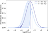Fig. 3 Disc mass distribution at 0.5 Myr and 2.5 Myr for the viscousphotoevaporative model (solid line), compared with purely viscous distributions (dashed line). The dotted vertical lines indicate the medians of the distributions of survived discs, while the hatched regions correspond to dispersed discs. This population has $\langle \log \left(M_0/{\text{M}}_{\odot }\right)\rangle =-2.5,\langle \log \left({\dot{M}}_0/{\text{M}}_{\odot }{\text{yr}}^{-1}\right)\rangle =-8.3$, and $\langle \log \left({\dot{M}}_{\text{w}}/{\text{M}}_{\odot }{\text{yr}}^{-1}\right)\rangle =-9.6$, where all quantities follow log-normal distributions with σ = 0.5 dex.

2.5 The effect of a correlation between the initial disc properties and M_⋆

As noted in Sect. 2.4.2, we find that the viscousphotoevaporative scenario predicts the median disc mass to increase with population age, regardless of the initial parameters chosen. We derived this feature by considering the scaling of the dispersal time with the initial mass, assuming that the other quantities do not depend on M₀. Here, we explore the impact of a correlation between the initial disc properties and the stellar mass on the results obtained in the previous section.

Numerous surveys of star-forming regions (see Manara et al. 2023 for a review) reveal a pronounced correlation between the disc mass, obtained from the sub-mm continuum emission of the dust component, the accretion rate, and the stellar mass. In particular, discs around massive stars tend to be more massive and higher accretors. Such correlations may be induced by disc evolution or may be due to initial conditions. Somigliana et al. (2022) explored the latter scenario by generating synthetic populations where M₀ and ${\dot{M}}_{\text{\hspace{0.17em}0\hspace{0.17em}}}$ are correlated with M_★ by power-law relations given by $$M_0\propto M_{\star }{}^{{\lambda }_{\text{m},0}},$$(20) $${\dot{M}}_0\propto M_{\star }{}^{{\lambda }_{\text{acc},0}}.$$(21)

Furthermore, numerical simulations (Picogna et al. 2021) highlight that discs surrounding massive stars experience a more intense wind mass-loss, correlated with M_⋆ through a power-law relation, $${\dot{M}}_{\text{w}}\propto M_{\star }{}^{{\lambda }_{\text{w}}},$$(22)

where we did not label λ_w with the subscript ‘0’ because in our model ${\dot{M}}_{\text{w}}$ is constant throughout the disc’s lifetime. Observational and theoretical constraints result in positive exponents, meaning that discs around massive stars tend to not only be more massive but also experience higher mass-loss due to both accretion and internal photoevaporation. This may imply that, although they have a larger initial mass, they may be shorterlived due to a more vigorous wind.

To assess whether the increase in the median disc mass would also occur in the viscous-photoevaporative model if we include a scaling of these properties with M_⋆, we substituted the power-law relations (20), (21), and (22) into the equations for the dispersal time, (8) and (11), and obtained the scaling of t_disp with M₀: $$t_{\text{disp}}\propto M_0{}^{\lambda },$$(23)

where $$\lambda =\{\begin{array}{cc}\frac{3{\lambda }_{\text{m},0}-{\lambda }_{\text{acc},0}-2{\lambda }_{\text{w}}}{3{\lambda }_{\text{m},0}}& \text{for the global criterion}\\ \frac{3+3{\lambda }_{\text{m},0}-{\lambda }_{\text{acc},0}-2{\lambda }_{\text{w}}}{5{\lambda }_{\text{m},0}}& \text{for the local criterion}.\end{array}$$(24)

Light discs are the first to be depleted only if λ > 0. However, as shown in Sect. 2.4.2, to allow the median mass to increase with time, M_0,MIN must scale with a steeper power law of t_disp than accretion. This condition is met when 0 < λ < 2 (see Eq. (15)). Hence, the slopes of the initial correlations with M_⋆ play a crucial role in determining whether the median mass of a population increases with time. To investigate whether this trend can be reproduced, we now consider an example based on the plausible values of the slopes reported in the literature. Specifically, following the constraints of Somigliana et al. (2022), who studied the evolution of the slopes of the correlations in synthetic populations of viscously accreting discs, we can assume that λ_m,0 and λ_acc,0 are in the following ranges: $${\lambda }_{\text{m},0}\in [1.2,2.1],$$(25) $${\lambda }_{\text{acc},0}\in [0.7,1.5].$$(26)

Moreover, Somigliana et al. (2022) find that, in order to reproduce the observed evolution of the slopes of the M–M_⋆ and $\dot{M}-M_{\star }$ correlations, λ_m,0 needs to be larger than λ_acc,0. Concerning the ${\dot{M}}_{\text{w}}$ correlation, we can assume λ_w ∼ 1, following Picogna et al. (2021). With these constraints, we find that the condition 0 < λ < 2, which is necessary to explain the increased median disc mass of surviving discs, still holds for both dispersal criteria.

In these sections, we highlight how assuming rapid inner disc clearing caused by internal photoevaporation results in an increase in the median mass of the population over time. Such a feature is expected in the simplest scenario, when $M_0,{\dot{M}}_0$, and ${\dot{M}}_{\text{w}}$ are not correlated with M_⋆. Moreover, the constraints on the slopes, λ_i, provided by the literature suggest that the increase in the median mass is a property of the viscous-photoevaporative model, even when the initial disc properties are correlated with stellar mass. In the next section, we support this statement with numerical simulations and discuss its implications.

3 Numerical simulations with Diskpop

The analytical arguments presented in Sect. 2 rely on two main assumptions: first, that photoevaporation does not affect the disc evolution until t_disp, at which point it instantly depletes the disc; and second, that the disc mass and accretion rate are distributed log-normally at age zero. In this section we show that populations of discs numerically evolved with the viscousphotoevaporative model, without relying on our first assumption, still manifest an increasing median mass.

We used the 1D code Diskpop, presented by Somigliana et al. (2024), which is designed to generate synthetic populations of discs. We generated an initial population of young stellar objects (YSOs), each of which consists of a star and a disc. We extracted the stellar mass, M_⋆, from an initial mass function (IMF), which, in Diskpop, can be selected from various options. The key initial parameters of the disc ($M_0,{\dot{M}}_0$, and ${\dot{M}}_{\text{w}}$) were extracted from log-normal distributions, with means determined by power-law correlations with M_⋆ (see Eqs. (20), (21) and (22)). Diskpop allows the selection of normalisations of the power laws – i.e. the values of $M_0,{\dot{M}}_0$, and ${\dot{M}}_{\text{w}}$ for a disc surrounding a 0.3 M_⊙ star (which, in our case, are also the mean values of the distributions) – as well as the exponents, λ_i, and the spreads, σ_i. The code solves the evolution, Eq. (1), for each disc and returns the values of Σ, M, and $\dot{M}$ at different snapshots. We imposed a threshold of 10⁻¹² M_⊙ yr⁻¹ for the accretion rate, based on observational detectability (Fedele et al. 2010), as well as a threshold for the disc mass of 10⁻⁶ M_⊙. If either ^$\dot{M}$ or M decreased below its respective threshold, the synthetic YSO was assumed to transition to Class III and was removed from the disc population. We chose α = 10⁻³ for all discs in the population.

3.1 Verifying the analytical predictions

We used Diskpop in order to verify whether the maximum between t_loc (see Eq. (8)) and t_w (see Eq. (11)) predicts the disc lifetime of synthetic discs and that a population that evolves according to Eq. (1) can be effectively described by the analytical distribution (19). To achieve this, we implemented the same initial conditions used to derive the analytical relation. Hence, we generated a population of 200 YSOs and extracted the stellar mass from a log-normal distribution centred at 0.3 M_⊙ with σ = 0.5 dex. For each YSO, we obtained the disc properties $M_0,{\dot{M}}_0$, and ${\dot{M}}_{\text{w}}$ using the procedure described previously, but choosing a null spread for all parameters. This resulted in a fictional population in which all disc properties were perfectly correlated with M_⋆. We chose λ_m,0 = 2, λ_acc,0 = 1, and λ_w = 1. The physical meaning of these correlations is that discs surrounding massive stars are more massive, have higher accretion rates, and experience higher mass-loss due to internal photoevaporation. We know from Eqs. (24) that this combination satisfies 0 < λ < 2 for both t_w and t_loc, resulting in massive discs having a longer lifetime. We subsequently evolved the population until 15 Myr, removing YSOs with accretion rates or masses below the imposed thresholds.

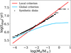Fig. 4 Comparison between the synthetic disc lifetime as a function of M0 and the analytical prediction.

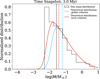Fig. 5 Comparison between the synthetic mass distribution and the analytical prediction for both dispersal criteria. The vertical lines represent the medians of each distribution.

3.1.1 Verifying the disc dispersal criterion

We show in Fig. 4 that the dispersal time of synthetic discs follows the analytical prediction. The plot shows that massive discs follow the local criterion, while light discs follow the global criterion. The presence of a regime switch emphasises the accuracy of our model. In this case, the lifetime of the majority of the discs is best approximated by the local criterion, although this can be reversed considering a different combination of initial conditions.

3.1.2 Verifying the analytical mass distribution

Figure 5 illustrates that the mass distribution of simulated discs aligns with the analytical prediction for both dispersal criteria. The distribution is strongly skewed since light discs are the first to be removed. Furthermore, the median of the surviving discs in the synthetic population increases with time, following analytical expectations (see Fig. 6). At early evolutionary stages (t < 1 Myr), the distribution is more accurately described by the global criterion; however, this relationship reverses at later stages. This occurs because the lifetime of light discs is better approximated by the global criterion, while massive discs tend to follow the local criterion (see Fig. 4). Figure 6 also highlights a discrepancy between the model and the simulations at very early stages (t ≪ 1 Myr), where the initial decrease in median mass due to viscous depletion is less steep in the simulations than predicted by the analytical expectations. This discrepancy arises because we derived m_0,MIN (see Eqs. (17) and (18)) under the assumption that t ≫ t_ν. Given that t_ν typically ranges from 10⁵ to 10⁶ yr, the analytical distribution only describes evolved populations. We performed additional simulations, varying the slopes, λ_i, and the normalisations of initial conditions, and confirmed that the increase in the median mass occurs only when predicted by the analytical model.

These simulations show that the evolution of the disc mass in populations evolved with the viscous-photoevaporative model is described by Eq. (19).

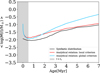Fig. 6 Comparison of the evolution of the median of the synthetic mass distribution over time with the analytical prediction for both dispersal criteria. The shaded region corresponds to t < tν, which is not considered in the model.

3.2 Generating a realistic disc population

In the previous section, we generated a population with ad hoc initial conditions to verify the results obtained analytically. In this section, we use Diskpop for its intended purpose: generating realistic synthetic disc populations. We show that the distinctive feature of the viscous-photoevaporative model presented in Sect. 2 likewise presents itself when more plausible initial distributions are implemented. First, for 200 discs, we extracted M_⋆ from the Kroupa IMF (Kroupa 2001), which, unlike the log-normal distribution used previously, favours lower stellar masses. As for disc parameters distributions, we set the slopes to λ_m,0 = 2, λ_acc,0 = 1, and λ_w = 1, with a spread of 0.5 dex. To ensure that our synthetic population matched the observed fraction of discs as a function of age (Hernández et al. 2007; Fedele et al. 2010), which indicates an average disc lifetime of 2–3 Myr, we tailored the normalisation of the initial correlations so that ⟨t_loc⟩ ∼ 2.5 Myr. Equation (11) demonstrates that an infinite number of combinations can satisfy this condition. Among all the possible combinations, we chose the following set of parameters:$\langle M_0\rangle =5\cdot {10}^{-3}{\text{M}}_{\odot },\langle {\dot{M}}_0\rangle =5\cdot {10}^{-9}{\text{M}}_{\odot }{\text{yr}}^{-1}$, and $\langle {\dot{M}}_{\text{w}}\rangle =6\cdot {10}^{-10}{\text{M}}_{\odot }{\text{yr}}^{-1}$. This choice not only satisfies the constraint that we imposed on t_loc, but also allows us to qualitatively reproduce the observed disc masses and accretion rates. However, we verified that any other combination would have equally served the purpose of this section.

We expected the steepest increase in median mass to occur between 2 and 4 Myr, the interval during which most of the discs are dispersed. We find that the generated population continues to manifest an increase in median mass over time. Figure 7 illustrates the mass distribution of the population at 3 and 4 Myr, highlighting the increasing median. The discs dispersed between these two time snapshots, which are shown in grey, are the least massive in the population. Hence, the removal of these low-mass discs causes the older population to appear more massive than the younger one. Further evidence of the key role of internal photoevaporation in this scenario is brought to light in Fig. 8, which depicts the population in the $\dot{M}-M$ plane. The disc distribution in the plane is compared to the viscous isochrone (Lodato et al. 2017), which is the locus of points in the plane that the discs would occupy if their evolution were driven purely by viscous accretion. Discs dispersed between 3 and 4 Myr (grey crosses) are below the curve, showing their $\dot{M}$ decreases faster than M, whereas the purely viscous theory predicts a linear correlation between the two. This feature is a hallmark of the internal photoevaporation predicted by Jones et al. (2012) and Rosotti et al. (2017) and found by Somigliana et al. (2020) in numerical simulations. Consequently, the fact that synthetic discs that show this behaviour are dispersed in the subsequent time snapshot highlights that internal photoevaporation is responsible for both their depletion and the increase of the median mass. The fact that the accretion rate decreases more steeply than the mass, due to both accretion and internal photoevaporation, causes the median of the accretion rate distribution to decline over time. This is highlighted in Fig. 9, which shows the evolution of the median disc mass and the median accretion rate over time for the synthetic population studied in this section. The decline in the accretion rate with population age is in agreement with observations (Testi et al. 2022). This survivorship bias, thus, is a specific property of the disc mass distribution.

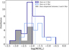Fig. 7 Histogram of the disc mass distribution at 3 Myr (dark blue) and 4 Myr (light blue). The dashed vertical lines indicate the medians of the distributions. The shaded histogram represents the mass distribution of discs dispersed between 3 and 4 Myr.

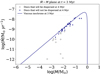Fig. 8 Population in the $\dot{M}-M$ plane at 3 Myr, compared to the viscous isochrone. Blue diamonds represent discs that are not dispersed at 4 Myr, while grey crosses represent discs that are dispersed at 4 Myr. The former correspond to the shaded histogram in Fig. 7.

Fig. 9 Evolution of the median disc mass (solid black line) and the median accretion rate (dashed blue line) over time with shaded regions representing the one-sigma confidence intervals of the population. The fraction of accreting discs at each timestep is shown above the plot.

4 Discussion

4.1 Is the increase with time of the median mass a general feature of viscous-photoevaporative models?

In Sect. 2.5 we illustrate the crucial impact of the slopes, λ_i, in governing the correlations between the initial disc conditions and M_⋆, noting that for 0 < λ < 2 (with λ as defined in Eq. (24)), the median disc mass increases with time. However, although some constraints of λ_i exist in the literature (Picogna et al. 2021; Somigliana et al. 2022), they are not robust enough to rule out the possibility that λ < 0 or λ > 2, scenarios in which the increase in median mass does not occur. In particular, the total mass-loss rate, ${\dot{M}}_{\text{w}}$, has been obtained for a restricted sample of discs (see Pascucci et al. 2023 for a recent review), which results in λ_w being observationally unconstrained. To properly evaluate which values of λ_i most accurately reproduce the observed populations, one would need to conduct a population synthesis model with a robust statistical method to compare simulations with data. Here we explore the impact of λ_w in determining whether the increase of M is a distinctive signature of this model.

The positive correlation between the X-ray luminosity and the stellar mass (Preibisch et al. 2005; Güdel et al. 2007; Ercolano et al. 2014) suggests that negative λ_w values are not physically meaningful for low mass stars (<1.5 M_⊙) for X-ray models. If we restrict to the Somigliana et al. (2022) and Somigliana et al. (2024) constraints on λ_m,0 and λ_acc,0 (see Sect. 2.5), and λ_w > 0, we find that no combination allows λ > 2 for either dispersal criteria. However, it is possible to obtain λ < 0, a condition under which massive discs are the first to be dispersed. We focused on the global criterion to determine the range of λ_w for which the condition 0 < λ < 2 holds, because we find that, if this is the case, the condition also holds for the local criterion. By assuming λ_m,0 = 2.1 and λ_acc,0 = 1.5, which are the upper boundaries of the assumed constraints, we find that λ < 0 occurs only when λ_w > 2.4 – a rather steep ${\dot{M}}_{\text{w}}-M_{\star }$ correlation, not currently predicted by numerical simulations (Picogna et al. 2021). Nevertheless, if we consider λ_m,0 = 1.2 and λ_acc,0 = 1.2, the combination within the Somigliana et al. (2022) constraints for which λ is lower, we obtain a limit value of λ_w = 1.2, which is close to the λ_w ∼ 1 predicted by Picogna et al. (2021). This suggests that a scenario where the median mass decreases with time cannot be completely excluded. We can obtain additional constraints by considering the R_obs–M_⋆ correlation, where R_obs is the disc radius observed in the mm flux. This correlation has been somewhat overlooked in the literature due to its lower prominence compared to the other two correlations and the significant uncertainties associated with R_obs measurements (Ansdell et al. 2018; Rosotti et al. 2019). Andrews et al. (2018b) and Hendler et al. (2020) find that R_obs ∝ M_⋆^0.6, which implies that massive stars tend to host larger discs. Furthermore, we know that the initial disc radius follows the relation $$\left(\frac{R_0}{\text{au}}\right)=6\pi \alpha \left(\frac{t_v}{\text{yr}}\right){\left(\frac{h}{r}\right)}^2{\left(\frac{M_{\star }}{M_{\odot }}\right)}^{-1/2}$$(27)

from the viscous model, where h/r = H/R at R = 1 au, and at M_⋆ = 1 M_⊙. Here, we assume that α does not depend on the stellar mass. As a consequence, if we assume that the observed R_obs–M_⋆ correlation is due to the R₀ distribution, we obtain $${\lambda }_{\text{m},0}-{\lambda }_{\text{acc},0}\sim 1.$$(28)

With this information, we conclude that λ_w < 2.2 yields λ > 0, which corresponds to an increase in the median mass of the population. This value indicates that only steep ${\dot{M}}_{\text{w}}-M_{\star }$ correlations with λ_w > 2 can prevent light discs from being dispersed first in populations. As discussed in this section, numerical simulations currently predict flatter scalings of the mass-loss rate with M_⋆ and, therefore, such steep correlations are very unlikely. Thus, we can argue that, if viscosity drives accretion in discs and internal photoevaporation is responsible for their dispersal, older populations should appear more massive than younger ones due to the survivorship bias. However, we stress that this argument is based on the assumption that the observed flux radius traces the critical disc radius, R_c, which is non-trivial (see Rosotti et al. 2019 and Toci et al. 2021).

4.2 Outside-in dispersal

The model described so far accounts for viscous accretion and internal photoevaporation, with the assumption that dispersal proceeds from inside out. This assumption has been crucial in establishing that photoevaporation affects the accretion rate more than the disc mass (see Fig. 2) and, consequently, that disc mass evolution can be described by purely viscous relations until the moment of disc dispersal. This assumption allowed us to obtain an analytical relation (19) that accurately describes the evolution of the M distribution. However, there are cases when internal photoevaporation can trigger an outside-in dispersal. This feature is usually associated with external photo-evaporation (Clarke 2007; Haworth & Clarke 2019; Winter & Haworth 2022; Anania et al. 2024) but can occur even for internal photoevaporation (Ronco et al. 2024; Tabone et al. 2025). Figure 10 shows the evolution of the surface density of a disc affected by outside-in dispersal, triggered by internal photoevaporation.

In this particular case, with R₀ ∼ 10 au, winds induce massloss at large radii and deplete the outer region first. This results in a decreasing disc size and in the clearing of the disc from outside in. To explain the physical reason behind this feature, we need to evaluate the dependence of the local dispersal timescale, defined in Eq. (10), on R. We assumed that the wind’s massloss rate profile does not depend on the disc structure and always peaks at small radii (see Eq. (12)). As a consequence, the dependence of t_loc on R is introduced by the surface density profile (2). When the truncation radius is considerably high, t_loc has a minimum at R_gap, where R_gap is defined in Eq. (12). The location of this minimum does not depend on R₀ but on M_⋆. In compact discs, the surface density is truncated at small radii, where the local mass-loss rate is still significant. This induces a second local minimum at large radii in the profile of t_loc(R) (see Fig. 11). The disc undergoes an outside-in dispersal when the second local minimum becomes a global minimum. The only parameter that plays a key role here is the truncation radius, which appears in the exponential term of Eq. (2). From numerical simulations, we obtain the minimum radius, R^′, for which t_loc has a global minimum at R = R_gap. We find R^′ ∼ 26 au by taking into account the Owen et al. (2012) ${{\displaystyle \dot{\sum }}}_w$ profile. Less steep mass-loss profiles, such as the one obtained by Picogna et al. (2019), where a larger fraction of mass is removed at large radii, produce a higher limit radius R^′. Consequently, discs with $R_{\text{c}}<R^{\prime }\left(\frac{M_{\star }}{{\text{M}}_{\odot }}\right)$ at t = t_disp do not open a gap but are depleted from outside-in.

Determining whether disc depletion occurs via inside-out (I-O) or outside-in (O-I) dispersal is not only crucial to assert whether the mass distribution increases with time – a feature predicted assuming I-O dispersal – but also to understand if winds are prone to carve cavities in gaseous discs. Here, we derive an analytical relation that separates the two regimes. Let us consider the relation $$R_{\text{c}}\left(t_{\text{disp}}\right)<R^{\prime }\left(\frac{M_{\star }}{{\text{M}}_{\odot }}\right),$$(29)

the condition under which we expect O-I dispersal according to numerical simulations. We used the global criterion (see Eq. (8)) to evaluate t_disp, because the local criterion obtained assumes I-O dispersal, which is not valid in this scenario. We account for viscous spreading by substituting $$R_{\text{c}}\left(t_{\text{w}}\right)=R_0\left(1+\frac{t_{\text{w}}}{t_v}\right)$$(30)

if ${\dot{M}}_{\text{\hspace{0.17em}0\hspace{0.17em}}}>{\dot{M}}_{\text{w}}$, and R_c = R₀ otherwise. We substitute Eq. (30) in Eq. (29) and obtain the condition under which photoevaporation triggers an O-I dispersal in evolved discs: $$M_0<2{\dot{M}}_{\text{w}}{t}_v{\left(\frac{R^{\prime }}{R_0}\right)}^{3/2}{\left(\frac{M_{\star }}{{\text{M}}_{\odot }}\right)}^{3/2}.$$(31)

By substituting the typical values of disc parameters, the condition becomes $$\begin{array}{c}{M}_0<2.83\cdot {10}^{-3}\left(\frac{{\dot{M}}_{\text{w}}}{{10}^{-9}{\text{M}}_{\odot }{\text{yr}}^{-1}}\right){\left(\frac{\alpha }{{10}^{-3}}\right)}^{-1}{\left(\frac{h/r}{1/30}\right)}^{-2}\\ \times {\left(\frac{M_{\star }}{{\text{M}}_{\odot }}\right)}^2{\left(\frac{R_0}{20\text{\hspace{0.17em}au}}\right)}^{-1/2}{\left(\frac{R^{\prime }}{26\text{\hspace{0.17em}au}}\right)}^{3/2}{\text{M}}_{\odot }.\end{array}$$(32)

This relation highlights that the more compact and lighter the disc, the more likely it is to have O-I dispersal. Moreover, the dispersal pathway strongly depends on the stellar mass and the shape of the ${{\displaystyle \dot{\sum }}}_w$ profile. Equation (32) is consistent with the results of Tabone et al. (2025), who find, with Diskpop, that small discs (R₀ ∼ 10 au) undergo an O-I dispersal. It is also consistent with Ronco et al. (2024), who numerically find that O-I dispersal is typical for discs around massive stars, and with Coleman & Haworth (2022), who did not observe this feature for discs with R > 100 au, unless they were affected by external photoevaporation.

To evaluate the validity of Eq. (29), we performed different numerical simulations, varying only M₀ and R₀. We show in Fig. 12 that the analytical relation predicts the dispersal pathway with remarkable accuracy.

Then, we used Diskpop to analyse the mass evolution of a population where the majority of discs undergo O-I disc dispersal. This population has $\langle M_0\rangle =8\cdot {10}^{-3}{\text{M}}_{\odot },\langle {\dot{M}}_0\rangle =5\text{\hspace{0.17em}·\hspace{0.17em}}{10}^{-9}{\text{M}}_{\odot }{\text{yr}}^{-1},\langle {\dot{M}}_{\text{w}}\rangle =3\cdot {10}^{-9}{\text{M}}_{\odot }{\text{yr}}^{-1}$, and α = 10⁻⁴. We find that the mass distribution does not follow the analytical relation (19) (see Fig. 13).

Such disagreement is expected because O-I dispersal removes the outer regions first, thereby decreasing the disc mass faster than the accretion rate. Indeed, for these discs, the mass reaches its threshold before the accretion rate, in contrast to the result obtained for I-O dispersed discs (see Sect. 3.2). As a consequence, not only is the O-I dispersal slower than the I-O dispersal, but it also induces a mass decrease in the population, balancing the increase resulting from the removal of light discs. Thus, the median mass remains somewhat constant between 2 and 4 Myr. Figure 14 shows how the analysed population is distributed in the $\dot{M}-M$ plane. It highlights that discs nearing depletion have masses close to the threshold and are generally located above the viscous isochrone, a signature of O-I dispersal (Rosotti et al. 2017). In conclusion, whether photoevaporative dispersal occurs from inside-out or outside-in strongly impacts the evolution of disc mass. Understanding which dispersal pathway affects the observed disc populations is indeed essential.

Fig. 10 Evolution of Σ with time as a function of radius of a disc with M0 = 4 · 10−3 M⊙, R0 = 9.3 au, α = 10−3, and ${\dot{M}}_{\text{w}}=2.5\cdot {10}^{-9}{\text{M}}_{\odot }{\text{yr}}^{-1}$. For this specific disc, internal photoevaporation is more effective in the outer regions, resulting in an outside-in dispersal.

Fig. 11 Local dispersal timescale as a function of radius for a disc with R0 = 63 au and for a disc with R0 = 23 au around a 1 M⊙ star.

Fig. 12 Numerical test of Eq. (32). The colours represent the regions of the R0–M0 plane where numerical discs are dispersed from outside-in (in yellow) or from inside-out (in blue). The dotted line represents the analytical boundary between these two regimes.

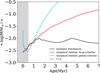Fig. 13 Comparison of the evolution of the median mass over time for the numerically evolved population and the analytical predictions for both dispersal criteria. The shaded region corresponds to t < tν, which is not considered in the model.

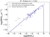Fig. 14 Population in the $\dot{M}-M$ plane at 3 Myr, compared with the viscous isochrone. Blue diamonds represent discs that are not dispersed at 4 Myr, while grey crosses represent discs that are dispersed at 4 Myr.

4.3 Comparison with the MHD wind model

Unlike the viscous framework, the MHD wind model explicitly defines dispersal time as the moment when both M and $\dot{M}$ vanish (Tabone et al. 2022a). This timescale depends on t_acc,0, a parameter that quantifies the accretion timescale. A priori, this parameter is not correlated with M₀, which means that this model does not inherently predict a longer lifetime for massive discs. Consequently, Tabone et al. (2022b) developed a population synthesis model where M₀ and t_acc,0 were extracted from independent distributions. They find that median mass distribution decreases with population age, because all discs lose mass through accretion. However, these results may change if there is an ad hoc correlation M₀–t_acc,0 such that $$M_0\propto t_{\text{acc},0}{}^{\varphi },$$(33) with ϕ > 0. This would imply that lighter discs have a shorter lifetime. To explore this possibility, we simulated a population evolved with the MHD model, with the same model parameters as those used by Zallio et al. (2024) and a correlation between M₀ and t_acc,0. We find that only positive correlations with ϕ > 0.5 cause the median mass to increase with time (see Fig. 15). However, ϕ > 0.5 is only marginally consistent with the results of Zallio et al. (2024), who find that, in order to reproduce the observed $\dot{M}-M$ correlation and the spread in M, MHD wind models must have ϕ ∈ [− 2, 1] (see Fig. 12 of Zallio et al. 2024). Therefore, we conclude that although an increase is not completely ruled out, the region of the allowed parameter space where MHD wind models predict an increasing median disc mass is narrow.

4.4 A new method for understanding disc evolution from observed populations

Throughout this work, we show that three different evolutionary pathways lead to three distinct signatures in the evolution of the median disc mass with time. Indeed, the viscous framework generally predicts an increase in the median mass in the case of inside-out I-O dispersal, and a constant median mass in the case of O-I dispersal, whereas MHD wind-driven accretion generally produces a decrease in these quantities over time. This raises the question of whether observations of disc mass can shed light on the evolutionary mechanism that drives accretion.

The analytical model, described in Sect. 2.4.2, predicts an increase in the median mass once most discs are removed from the population, which occurs at 2–3 Myr (Hernández et al. 2007; Fedele et al. 2010). Therefore, our theoretical model predicts that this feature is distinguishable between 2 and 4–6 Myr, during which we expect the median mass to increase by more than 0.5 dex (see Fig. 6). Since the median mass is less influenced by outliers than the global mass distribution, this method is less affected by sample incompleteness compared to others (see e.g. Alexander et al. 2023; Somigliana et al. 2024). As a result, we expect it to provide constraints also for samples of ∼ 100 discs. Consequently, a comparison between the median mass of ‘young’ populations, such as Lupus and Chamaeleon, with t ∼ 2 Myr (Luhman 2020; Galli et al. 2021), and ‘old’ populations, such as Upper-Sco, with 5–10 Myr (Pecaut & Mamajek 2016), is ideal for probing the accretion mechanism. Testi et al. (2022) observe an increase in the continuum flux from 1 Myr to 2 Myr, followed by a decrease from 2 Myr to 5 Myr, which hints that the dust mass somewhat increases in the earliest phase of disc evolution. The authors interpret this trend as a secondary dust production. Nevertheless, converting from continuum flux to gas mass remains non-trivial (see Miotello et al. 2023 for a review), suggesting that gas measurements can probe the evolution of total disc mass more accurately. Furthermore, different star-forming regions can be compared only if they can be described by the same initial conditions (see Zagaria et al. 2023). To retrieve this information, we would need to implement a robust statistical method to compare synthetic populations with observed ones. Moreover, as shown by Anania et al. (2024), irradiation from massive stars produces non-negligible effects on the evolution of disc sizes and masses in Upper-Sco, where both these quantities are reduced compared to the non-irradiated case. Therefore, external photoevaporation must be included in the model to reproduce such star-forming regions. New large programmes, such as AGE-PRO and DECO, will allow us to compare the expected evolution of the gas mass to the observed one.

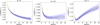Fig. 15 Evolution of the median mass as a function of time for two sets of populations evolved according to the MHD wind model, with ϕ = 0 (left panel), ϕ = 0.5 (central panel), and ϕ = 1 (right panel). The gold lines represent the medians of all the simulations with the same ϕ value.

4.5 Caveats about ${{\displaystyle \dot{\sum }}}_w$ and α

In this section, we discuss the assumptions made throughout the paper about ${{\displaystyle \dot{\sum }}}_w$ and α. We assumed that the mass-loss rate does not depend on time and on the structure of the disc, following Owen et al. (2012). However, Nakatani et al. (2021) find that the X-ray luminosity of pre-main-sequence stars can decrease by some order of magnitude as soon as the star enters the main sequence. This effect is more pronounced for stars with M_⋆ > 1 M_⊙, while it remains negligible for T-Tauri stars, which we studied in this work. Moreover, more recent mass-loss profiles (Picogna et al. 2019; Nakatani & Takasao 2022; Sellek et al. 2024) suggest that ${{\displaystyle \dot{\sum }}}_w$ should not be independent of the disc parameters. In particular, the mass-loss rate falls at R > R_c, suggesting that our analytical relation (31) might overestimate the number of discs dispersed from the outside in populations. However, to quantify the discrepancy between our model and more refined calculations, the dependence of ${{\displaystyle \dot{\sum }}}_w$ on R_c should be investigated through numerical simulations. We foresee future implementations of the updated ${{\displaystyle \dot{\sum }}}_w$ profiles in Diskpop. In addition, although we separated MHD winds and photoevaporation in order to isolate their effects, these phenomena (as well as turbulence and MHD winds) are not mutually exclusive and can be simultaneously present in discs. Future studies must consider this assumption and examine the effect of a hybrid model on the evolution of the disc mass distribution.

Throughout this work, we assumed α to be constant with respect to radius and stellar mass. Gárate et al. (2021) and Tong et al. (2024) explored the presence of a dead zone with small α at low radii. They find a significant increase in the lifetime of the inner disc. We expect such a feature to slow the decrease in $\dot{M}$ after the opening of the cavity and to lead to a slightly less steep increase in the median mass. Various studies (e.g. Gorti et al. 2009; Kunitomo et al. 2021) have introduced an α∝ M_⋆ scaling. This linear correlation affects the local criterion (11), which depends directly on α, as well as the global criterion, since t_ν = t_ν(α). As a consequence, if this correlation existed, the constraint from R_obs would become λ_m,0 − λ_acc,0 ∼ 0, further reducing the parameter region where an increase in median mass is expected. Finally, we stress that our work does not account for planet-disc interactions, which become significant if protoplanets had already formed by t ∼ 2 Myr.

5 Conclusions

In this paper, we have explored the evolution of the mass distribution of a protoplanetary disc population that evolves according to the viscous-photoevaporative framework. We derived an analytical relation that describes it and discussed its physical meaning. To verify these analytical predictions, we performed various numerical simulations with Diskpop (Somigliana et al. 2024) and confirmed our expectations. Then, we compared our results with different evolutionary pathways, such as O-I photoevaporative dispersal and MHD wind evolution. Our main results are the following:

1. Populations evolving under viscous accretion and undergoing I-O dispersal driven by internal photoevaporation exhibit a unique feature: an apparent increase in median disc mass over time. This occurs because lighter discs are the first to be dispersed by internal photoevaporation. This form of survivorship bias is manifested by populations where disc properties are independent of each other. Across a broad region of the parameter space, it also occurs in populations where each quantity correlates with the stellar mass. An increase in the median disc mass does not imply a rise in median mass accretion rates in populations. Rather, the accretion rate declines over time;

2. Other evolutionary pathways do not exhibit the same evolution of the median disc mass. In particular, an O-I dispersal results in the median mass remaining somewhat constant over time, while the MHD wind model in general predicts it to decrease with time. Such a difference highlights that the increase in the median mass is a signature of the viscous-photoevaporative model with I-O dispersal;

3. We derived a new criterion to estimate the disc’s lifetime as a function of initial disc properties. We further derived an analytical relation that predicts that internal photoevaporation triggers I-O (O-I) disc dispersal if its critical radius at the moment of dispersal is larger (smaller) than a numerically determined threshold. We verified both analytical relations with numerically evolved synthetic populations;

4. We propose a new method for distinguishing between the viscous-photoevaporative and MHD wind-driven evolution in observations. Indeed, comparing the mass distribution of 2 Myr-old observed populations, such as Lupus, with older populations, such as Upper-Sco, could help disentangle the accretion mechanism. The recent large programs AGEPRO and DECO, which aim to expand the sample of gas masses in disc populations, provide a valuable opportunity to do this.

Future studies should focus on providing a statistically robust comparison between observed populations and theoretical expectations. This will enable us to verify if young and old star-forming regions are comparable. Moreover, measuring disc masses with more accuracy and precision (see for example Lodato et al. 2023; Martire et al. 2024) will be crucial for understanding disc evolution.

Acknowledgements

We thank the anonymous referee for the comments that improved the clarity of this paper. The authors acknowledge support from the European Union (ERC Starting Grant DiscEvol, project number 101039651 and ERC, WANDA, project number 101039452), from Fondazione Cariplo, grant No. 2022-1217, from the European Union’s Horizon 2020 research and innovation programme under the Marie Sklodowska-Curie grant agreement No. 823823 (Dustbusters RISE project), and from the ERC Synergy Grant “ECOGAL” (project ID 855130). Views and opinions expressed are, however, those of the authors only and do not necessarily reflect those of the European Union or the European Research Council. Neither the European Union nor the granting authority can be held responsible for them. Part of this work was supported by the European Southern Observatory (ESO) who funded LM for a threemonth internship. GL acknowledges financial contribution from PRIN-MUR 20228JPA3A. Moreover, we thank Cathie Clarke and Giovanni Picogna for the insightful discussions and very useful comments.

Appendix A Derivation of the analytical mass distribution

Here we show how we derived the analytical mass distribution (see Figure 3). Let us consider equation (19), where $$\frac{\partial N}{\partial m_0}=N_1\exp \left(-\frac{{\left(m_0-\overline{m_0}\right)}^2}{2{\sigma }_{m_0}^2}\right)$$(A.1)

and $$\frac{\partial N}{\partial {\dot{m}}_0}=N_2\exp \left(-\frac{{\left({\dot{m}}_0-\overline{{\dot{m}}_0}\right)}^2}{2{\sigma }_{{\dot{m}}_0}^2}\right).$$(A.2)

The relation becomes $$\frac{\partial N}{\partial m}=N_1{N}_2{{{\displaystyle \int }}^{\text{}}}_{m_{0,\text{MIN}}}^{+\infty }\text{d}{\tilde{\text{m}}}_0\exp \left(-\frac{1}{2}ℳ\right),$$(A.3)

with $$ℳ=\frac{{\tilde{m}}_0^2}{\sigma m_0{}^2}+\frac{9}{\sigma {\dot{m}}_0{}^2}{\left({\tilde{m}}_0-\frac{2}{3}\tilde{m}\right)}^2,$$(A.4)

$\tilde{m}0\equiv m_0-\overline{m_0}$ and $\tilde{m}\equiv m-\overline{m}$. Following Somigliana et al. (2022), we isolate the dependence of the integration variable $\tilde{m}0$, so that we can move the term that depends only on $\tilde{m}$ out of the integral; $$\frac{\partial N}{\partial m}=N_3\exp \left(-\frac{{\tilde{m}}^2}{2{\sigma }^2}\right)\cdot {{{\displaystyle \int }}^{\text{}}}_{{\tilde{m}}_{0, \text{MIN} }}^{+\infty }\text{d}{\tilde{m}}_0\exp \left[-\frac{1}{2}{\left(A{\tilde{m}}_0-\frac{2}{3}\frac{B^2}{A}\tilde{m}\right)}^2\right],$$(A.5)

where ${\sigma }^2=\frac{9}{4}{\sigma }_{m_0}{}^2+\frac{1}{4}{\sigma }_{{\dot{m}}_0}{}^2,A^2=\frac{1}{{\sigma }_{m_0}{}^2}+\frac{9}{{\sigma }_{{\dot{m}}_0}{}^2}$ and $B^2=\frac{9}{{\sigma }_{{\dot{m}}_0}{}^2}$.

We notice that the exponential term outside the integral matches to the one obtained by Somigliana et al. (2022) considering the purely viscous model. This term represents a Gaussian distribution whose mean is constantly decreasing with time due to accretion. Instead, photoevaporation only introduces a minimum initial mass m_0,MIN, without which the second term would be a mere multiplicative constant. After some straightforward integration we obtain $$\begin{array}{l}\frac{\partial N}{\partial m}=N_3\exp \left(-\frac{{(m-\overline{m}(t))}^2}{2{\sigma }^2}\right)\times \\ \times \sqrt{\frac{\pi }{2}}\frac{1-erf\left[\frac{1}{\sqrt{2}}A\left(m_{0,\text{MIN}}(t)-m_0\right)-\frac{2}{3}\frac{B^2}{A}(m-\overline{m})\right]}{A}.\end{array}$$(A.6)

References

All Figures

	Fig. 1 Evolution of the surface density of a disc over time, obtained by integrating Eq. (1) using Diskpop. This disc has M0 = 1.5 · 10−2 M⊙, R0 = 32.8 au, α = 10−3, and ${\dot{M}}_{\text{w}}=2.5\cdot {10}^{-9}{\text{M}}_{\odot }{\text{yr}}^{-1}$. After the opening of the gap, the inner disc is dispersed on a short timescale.
In the text

	Fig. 2 Evolution of the accretion rate (blue) and mass (black) of a disc over time. The vertical yellow line indicates the instant when the gap opens, which triggers a steep decrease in $\dot{M}$. The red line marks the transition between accreting and non-accreting phases. The grey region corresponds to values of disc mass and accretion rate below the respective observational threshold.
In the text

Fig. 3 Disc mass distribution at 0.5 Myr and 2.5 Myr for the viscousphotoevaporative model (solid line), compared with purely viscous distributions (dashed line). The dotted vertical lines indicate the medians of the distributions of survived discs, while the hatched regions correspond to dispersed discs. This population has $\langle \log \left(M_0/{\text{M}}_{\odot }\right)\rangle =-2.5,\langle \log \left({\dot{M}}_0/{\text{M}}_{\odot }{\text{yr}}^{-1}\right)\rangle =-8.3$, and $\langle \log \left({\dot{M}}_{\text{w}}/{\text{M}}_{\odot }{\text{yr}}^{-1}\right)\rangle =-9.6$, where all quantities follow log-normal distributions with σ = 0.5 dex.

In the text

	Fig. 4 Comparison between the synthetic disc lifetime as a function of M0 and the analytical prediction.
In the text

	Fig. 5 Comparison between the synthetic mass distribution and the analytical prediction for both dispersal criteria. The vertical lines represent the medians of each distribution.
In the text

	Fig. 6 Comparison of the evolution of the median of the synthetic mass distribution over time with the analytical prediction for both dispersal criteria. The shaded region corresponds to t < tν, which is not considered in the model.
In the text

	Fig. 7 Histogram of the disc mass distribution at 3 Myr (dark blue) and 4 Myr (light blue). The dashed vertical lines indicate the medians of the distributions. The shaded histogram represents the mass distribution of discs dispersed between 3 and 4 Myr.
In the text

	Fig. 8 Population in the $\dot{M}-M$ plane at 3 Myr, compared to the viscous isochrone. Blue diamonds represent discs that are not dispersed at 4 Myr, while grey crosses represent discs that are dispersed at 4 Myr. The former correspond to the shaded histogram in Fig. 7.
In the text

	Fig. 9 Evolution of the median disc mass (solid black line) and the median accretion rate (dashed blue line) over time with shaded regions representing the one-sigma confidence intervals of the population. The fraction of accreting discs at each timestep is shown above the plot.
In the text

	Fig. 10 Evolution of Σ with time as a function of radius of a disc with M0 = 4 · 10−3 M⊙, R0 = 9.3 au, α = 10−3, and ${\dot{M}}_{\text{w}}=2.5\cdot {10}^{-9}{\text{M}}_{\odot }{\text{yr}}^{-1}$. For this specific disc, internal photoevaporation is more effective in the outer regions, resulting in an outside-in dispersal.
In the text

	Fig. 11 Local dispersal timescale as a function of radius for a disc with R0 = 63 au and for a disc with R0 = 23 au around a 1 M⊙ star.
In the text

	Fig. 12 Numerical test of Eq. (32). The colours represent the regions of the R0–M0 plane where numerical discs are dispersed from outside-in (in yellow) or from inside-out (in blue). The dotted line represents the analytical boundary between these two regimes.
In the text

	Fig. 13 Comparison of the evolution of the median mass over time for the numerically evolved population and the analytical predictions for both dispersal criteria. The shaded region corresponds to t < tν, which is not considered in the model.
In the text

	Fig. 14 Population in the $\dot{M}-M$ plane at 3 Myr, compared with the viscous isochrone. Blue diamonds represent discs that are not dispersed at 4 Myr, while grey crosses represent discs that are dispersed at 4 Myr.
In the text

	Fig. 15 Evolution of the median mass as a function of time for two sets of populations evolved according to the MHD wind model, with ϕ = 0 (left panel), ϕ = 0.5 (central panel), and ϕ = 1 (right panel). The gold lines represent the medians of all the simulations with the same ϕ value.
In the text

References

- Alcalá, J. M., Natta, A., Manara, C. F., et al. 2014, A&A, 561, A2 [NASA ADS] [CrossRef] [EDP Sciences] [Google Scholar]
- Alcalá, J. M., Manara, C. F., Natta, A., et al. 2017, A&A, 600, A20 [NASA ADS] [CrossRef] [EDP Sciences] [Google Scholar]
- Alexander, R. D., & Armitage, P. J. 2009, ApJ, 704, 989 [Google Scholar]
- Alexander, R. D., Clarke, C. J., & Pringle, J. E. 2006, MNRAS, 369, 216 [NASA ADS] [CrossRef] [Google Scholar]
- Alexander, R., Pascucci, I., Andrews, S., Armitage, P., & Cieza, L. 2014, in Protostars and Planets VI, eds. H. Beuther, R. S. Klessen, C. P. Dullemond, & T. Henning, 475 [Google Scholar]
- Alexander, R., Rosotti, G., Armitage, P. J., et al. 2023, MNRAS, 524, 3948 [NASA ADS] [CrossRef] [Google Scholar]
- Almendros-Abad, V., Manara, C. F., Testi, L., et al. 2024, A&A, 685, A118 [NASA ADS] [CrossRef] [EDP Sciences] [Google Scholar]
- Anania, R., Rosotti, G., & Pinilla, P. 2024, in EAS2024, 999 [Google Scholar]
- Andrews, S. M., Huang, J., Pérez, L. M., et al. 2018a, ApJ, 869, L41 [NASA ADS] [CrossRef] [Google Scholar]
- Andrews, S. M., Terrell, M., Tripathi, A., et al. 2018b, ApJ, 865, 157 [Google Scholar]
- Ansdell, M., Williams, J. P., van der Marel, N., et al. 2016, VizieR Online Data Catalog: J/ApJ/828/46 [Google Scholar]
- Ansdell, M., Williams, J. P., Manara, C. F., et al. 2017, VizieR Online Data Catalog: ALMA survey of protoplanetary disks in sigma Ori (Ansdell+, 2017), VizieR On-line Data Catalog: J/AJ/153/240. Originally published in: 2017AJ. 153.240A [Google Scholar]
- Ansdell, M., Williams, J. P., Trapman, L., et al. 2018, ApJ, 859, 21 [NASA ADS] [CrossRef] [Google Scholar]
- Barenfeld, S. A., Carpenter, J. M., Ricci, L., & Isella, A. 2016, ApJ, 827, 142 [Google Scholar]
- Bergin, E. A., & Williams, J. P. 2017, in Astrophysics and Space Science Library, 445, Formation, Evolution, and Dynamics of Young Solar Systems, eds. M. Pessah, & O. Gressel, 1 [Google Scholar]
- Blandford, R. D., & Payne, D. G. 1982, MNRAS, 199, 883 [CrossRef] [Google Scholar]
- Cazzoletti, P., Manara, C. F., Liu, H. B., et al. 2019, A&A, 626, A11 [NASA ADS] [CrossRef] [EDP Sciences] [Google Scholar]
- Clarke, C. J. 2007, MNRAS, 376, 1350 [NASA ADS] [CrossRef] [Google Scholar]
- Clarke, C. J., Gendrin, A., & Sotomayor, M. 2001, MNRAS, 328, 485 [NASA ADS] [CrossRef] [Google Scholar]
- Coleman, G. A. L., & Haworth, T. J. 2022, MNRAS, 514, 2315 [NASA ADS] [CrossRef] [Google Scholar]
- Coleman, G. A. L., Mroueh, J. K., & Haworth, T. J. 2024, MNRAS, 527, 7588 [Google Scholar]
- Delussu, L., Birnstiel, T., Miotello, A., et al. 2024, A&A, 688, A81 [NASA ADS] [CrossRef] [EDP Sciences] [Google Scholar]
- Ercolano, B., Mayr, D., Owen, J. E., Rosotti, G., & Manara, C. F. 2014, MNRAS, 439, 256 [NASA ADS] [CrossRef] [Google Scholar]
- Ercolano, B., & Pascucci, I. 2017, Roy. Soc. Open Sci., 4, 170114 [Google Scholar]
- Fedele, D., van den Ancker, M. E., Henning, T., Jayawardhana, R., & Oliveira, J. M. 2010, A&A, 510, A72 [NASA ADS] [CrossRef] [EDP Sciences] [Google Scholar]
- Font, A. S., McCarthy, I. G., Johnstone, D., & Ballantyne, D. R. 2004, ApJ, 607, 890 [NASA ADS] [CrossRef] [Google Scholar]
- Galli, P. A. B., Bouy, H., Olivares, J., et al. 2021, A&A, 646, A46 [NASA ADS] [CrossRef] [EDP Sciences] [Google Scholar]
- Gárate, M., Delage, T. N., Stadler, J., et al. 2021, A&A, 655, A18 [NASA ADS] [CrossRef] [EDP Sciences] [Google Scholar]
- Gorti, U., & Hollenbach, D. 2009, ApJ, 690, 1539 [Google Scholar]
- Gorti, U., Dullemond, C. P., & Hollenbach, D. 2009, ApJ, 705, 1237 [Google Scholar]
- Güdel, M., Briggs, K. R., Arzner, K., et al. 2007, A&A, 468, 353 [Google Scholar]
- Hartmann, L., Calvet, N., Gullbring, E., & D’Alessio, P. 1998, ApJ, 495, 385 [Google Scholar]
- Haworth, T. J., & Clarke, C. J. 2019, MNRAS, 485, 3895 [NASA ADS] [CrossRef] [Google Scholar]
- Hendler, N., Pascucci, I., Pinilla, P., et al. 2020, ApJ, 895, 126 [Google Scholar]
- Hernández, J., Hartmann, L., Megeath, T., et al. 2007, ApJ, 662, 1067 [Google Scholar]
- Hollenbach, D., Johnstone, D., Lizano, S., & Shu, F. 1994, ApJ, 428, 654 [NASA ADS] [CrossRef] [Google Scholar]
- Jones, M. G., Pringle, J. E., & Alexander, R. D. 2012, MNRAS, 419, 925 [NASA ADS] [CrossRef] [Google Scholar]
- Kroupa, P. 2001, MNRAS, 322, 231 [NASA ADS] [CrossRef] [Google Scholar]
- Kunitomo, M., Ida, S., Takeuchi, T., et al. 2021, ApJ, 909, 109 [NASA ADS] [CrossRef] [Google Scholar]
- Lesur, G. R. J. 2021, A&A, 650, A35 [NASA ADS] [CrossRef] [EDP Sciences] [Google Scholar]
- Lodato, G., Scardoni, C. E., Manara, C. F., & Testi, L. 2017, MNRAS, 472, 4700 [NASA ADS] [CrossRef] [Google Scholar]
- Lodato, G., Rampinelli, L., Viscardi, E., et al. 2023, MNRAS, 518, 4481 [Google Scholar]
- Luhman, K. L. 2020, AJ, 160, 186 [NASA ADS] [CrossRef] [Google Scholar]
- Lynden-Bell, D., & Pringle, J. E. 1974, MNRAS, 168, 603 [Google Scholar]
- Manara, C. F., Testi, L., Herczeg, G. J., et al. 2017, A&A, 604, A127 [NASA ADS] [CrossRef] [EDP Sciences] [Google Scholar]
- Manara, C. F., Ansdell, M., Rosotti, G. P., et al. 2023, in Astronomical Society of the Pacific Conference Series, 534, Protostars and Planets VII, eds. S. Inutsuka, Y. Aikawa, T. Muto, K. Tomida, & M. Tamura, 539 [NASA ADS] [Google Scholar]
- Martire, P., Longarini, C., Lodato, G., et al. 2024, A&A, 686, A9 [Google Scholar]
- Miotello, A., van Dishoeck, E. F., Kama, M., & Bruderer, S. 2016, A&A, 594, A85 [NASA ADS] [CrossRef] [EDP Sciences] [Google Scholar]
- Miotello, A., Kamp, I., Birnstiel, T., Cleeves, L. C., & Kataoka, A. 2023, in Astronomical Society of the Pacific Conference Series, 534, Protostars and Planets VII, eds. S. Inutsuka, Y. Aikawa, T. Muto, K. Tomida, & M. Tamura, 501 [NASA ADS] [Google Scholar]
- Mulders, G. D., Pascucci, I., Manara, C. F., et al. 2017, ApJ, 847, 31 [NASA ADS] [CrossRef] [Google Scholar]
- Najita, J. R., & Bergin, E. A. 2018, ApJ, 864, 168 [Google Scholar]
- Nakatani, R., & Takasao, S. 2022, ApJ, 930, 124 [Google Scholar]
- Nakatani, R., Hosokawa, T., Yoshida, N., Nomura, H., & Kuiper, R. 2018, ApJ, 865, 75 [Google Scholar]
- Nakatani, R., Kobayashi, H., Kuiper, R., Nomura, H., & Aikawa, Y. 2021, ApJ, 915, 90 [NASA ADS] [CrossRef] [Google Scholar]
- Owen, J. E., & Kollmeier, J. A. 2019, MNRAS, 487, 3702 [Google Scholar]
- Owen, J. E., Ercolano, B., Clarke, C. J., & Alexander, R. D. 2010, MNRAS, 401, 1415 [Google Scholar]
- Owen, J. E., Clarke, C. J., & Ercolano, B. 2012, MNRAS, 422, 1880 [Google Scholar]
- Pascucci, I., Cabrit, S., Edwards, S., et al. 2023, in Astronomical Society of the Pacific Conference Series, 534, Protostars and Planets VII, eds. S. Inutsuka, Y. Aikawa, T. Muto, K. Tomida, & M. Tamura, 567 [NASA ADS] [Google Scholar]
- Pecaut, M. J., & Mamajek, E. E. 2016, MNRAS, 461, 794 [Google Scholar]
- Picogna, G., Ercolano, B., Owen, J. E., & Weber, M. L. 2019, MNRAS, 487, 691 [Google Scholar]
- Picogna, G., Ercolano, B., & Espaillat, C. C. 2021, MNRAS, 508, 3611 [NASA ADS] [CrossRef] [Google Scholar]
- Preibisch, T., Kim, Y.-C., Favata, F., et al. 2005, ApJS, 160, 401 [NASA ADS] [CrossRef] [Google Scholar]
- Pringle, J. E. 1981, ARA&A, 19, 137 [NASA ADS] [CrossRef] [Google Scholar]
- Robinson, A., Owen, J. E., & Booth, R. A. 2025, MNRAS, 536, 1689 [Google Scholar]
- Ronco, M. P., Schreiber, M. R., Villaver, E., Guilera, O. M., & Miller Bertolami, M. M. 2024, A&A, 682, A155 [NASA ADS] [CrossRef] [EDP Sciences] [Google Scholar]
- Rosotti, G. P. 2023, New A Rev., 96, 101674 [Google Scholar]
- Rosotti, G. P., Clarke, C. J., Manara, C. F., & Facchini, S. 2017, MNRAS, 468, 1631 [NASA ADS] [Google Scholar]
- Rosotti, G. P., Tazzari, M., Booth, R. A., et al. 2019, MNRAS, 486, 4829 [NASA ADS] [CrossRef] [Google Scholar]
- Sanchis, E., Testi, L., Natta, A., et al. 2020, A&A, 633, A114 [NASA ADS] [CrossRef] [EDP Sciences] [Google Scholar]
- Sellek, A. D., Grassi, T., Picogna, G., et al. 2024, A&A, 690, A296 [NASA ADS] [CrossRef] [EDP Sciences] [Google Scholar]
- Shakura, N. I., & Sunyaev, R. A. 1973, A&A, 24, 337 [NASA ADS] [Google Scholar]
- Somigliana, A., Toci, C., Lodato, G., Rosotti, G., & Manara, C. F. 2020, MNRAS, 492, 1120 [NASA ADS] [CrossRef] [Google Scholar]
- Somigliana, A., Toci, C., Rosotti, G., et al. 2022, MNRAS, 514, 5927 [NASA ADS] [CrossRef] [Google Scholar]
- Somigliana, A., Testi, L., Rosotti, G., et al. 2023, ApJ, 954, L13 [NASA ADS] [CrossRef] [Google Scholar]
- Somigliana, A., Testi, L., Rosotti, G., et al. 2024, A&A, 689, A285 [NASA ADS] [CrossRef] [EDP Sciences] [Google Scholar]
- Tabone, B., Rosotti, G. P., Cridland, A. J., Armitage, P. J., & Lodato, G. 2022a, MNRAS, 512, 2290 [NASA ADS] [CrossRef] [Google Scholar]
- Tabone, B., Rosotti, G. P., Lodato, G., et al. 2022b, MNRAS, 512, L74 [NASA ADS] [CrossRef] [Google Scholar]
- Tabone, B., Rosotti, G. P., Trapman, L., et al. 2025, arXiv e-prints [arXiv:2506.10742] [Google Scholar]
- Tazzari, M., Testi, L., Natta, A., et al. 2017, A&A, 606, A88 [NASA ADS] [CrossRef] [EDP Sciences] [Google Scholar]
- Testi, L., Natta, A., Manara, C. F., et al. 2022, A&A, 663, A98 [NASA ADS] [CrossRef] [EDP Sciences] [Google Scholar]
- Toci, C., Rosotti, G., Lodato, G., Testi, L., & Trapman, L. 2021, MNRAS, 507, 818 [NASA ADS] [CrossRef] [Google Scholar]
- Toci, C., Lodato, G., Livio, F. G., Rosotti, G., & Trapman, L. 2023, MNRAS, 518, L69 [Google Scholar]
- Tong, S., Alexander, R., & Rosotti, G. 2024, MNRAS, 533, 1211 [Google Scholar]
- Trapman, L., Rosotti, G., Bosman, A. D., Hogerheijde, M. R., & van Dishoeck, E. F. 2020, A&A, 640, A5 [EDP Sciences] [Google Scholar]
- Trapman, L., Zhang, K., van’t Hoff, M., Hogerheijde, M., & Bergin, E. 2022, in American Astronomical Society Meeting Abstracts, 240, 319.03 [Google Scholar]
- Winter, A. J., & Haworth, T. J. 2022, Eur. Phys. J. Plus, 137, 1132 [NASA ADS] [CrossRef] [Google Scholar]
- Zagaria, F., Rosotti, G. P., Clarke, C. J., & Tabone, B. 2022, MNRAS, 514, 1088 [CrossRef] [Google Scholar]
- Zagaria, F., Facchini, S., Miotello, A., et al. 2023, A&A, 672, L15 [CrossRef] [EDP Sciences] [Google Scholar]
- Zallio, L., Rosotti, G., Tabone, B., et al. 2024, A&A, 692, A93 [NASA ADS] [CrossRef] [EDP Sciences] [Google Scholar]
The slight differences between our derivation and that by Somigliana et al. (2022) arise from the fact that we focus on the initial accretion rate rather than the viscous time.