Toward a population synthesis of disks and planets

Alexandre Emsenhuber; Remo Burn; Jesse Weder; Kristina Monsch; Giovanni Picogna; Barbara Ercolano; Thomas Preibisch

doi:10.1051/0004-6361/202244767

Home

All issues

Volume 673 (May 2023)

A&A, 673 (2023) A78

Full HTML

Open Access

Issue		A&A Volume 673, May 2023


Article Number		A78
Number of page(s)		18
Section		Planets and planetary systems
DOI		https://doi.org/10.1051/0004-6361/202244767
Published online		10 May 2023

A&A 673, A78 (2023)

II. Confronting disk models and observations at the population level^★

Alexandre Emsenhuber¹, Remo Burn², Jesse Weder³, Kristina Monsch⁴^,1, Giovanni Picogna¹, Barbara Ercolano¹^,5 and Thomas Preibisch¹

¹ Universitäts-Sternwarte, Ludwig-Maximilians-Universität München, Scheinerstraße 1, 81679 München, Germany
e-mail: emsenhuber@usm.lmu.de
² Max-Planck-Institut für Astronomie, Königstuhl 17, 69117 Heidelberg, Germany
³ Physikalisches Institut, Universität Bern, Gesellschaftsstrasse 6, 3012 Bern, Switzerland
⁴ Center for Astrophysics – Harvard & Smithsonian, 60 Garden Street, Cambridge, MA 02138, USA
⁵ Excellence Cluster ‘Origins’, Boltzmannstraße 2, 85748 Garching, Germany

Received: 18 August 2022
Accepted: 9 December 2022

Abstract

Aims. We want to find the distribution of initial conditions that best reproduces disc observations at the population level.

Methods. We first ran a parameter study using a 1D model that includes the viscous evolution of a gas disc, dust, and pebbles, coupled with an emission model to compute the millimetre flux observable with ALMA. This was used to train a machine learning surrogate model that can compute the relevant quantity for comparison with observations in seconds. This surrogate model was used to perform parameter studies and synthetic disc populations.

Results. Performing a parameter study, we find that internal photoevaporation leads to a lower dependency of disc lifetime on stellar mass than external photoevaporation. This dependence should be investigated in the future. Performing population synthesis, we find that under the combined losses of internal and external photoevaporation, discs are too short lived.

Conclusions. To match observational constraints, future models of disc evolution need to include one or a combination of the following processes: infall of material to replenish the discs, shielding of the disc from internal photoevaporation due to magnetically driven disc winds, and extinction of external high-energy radiation. Nevertheless, disc properties in low-external-photoevaporation regions can be reproduced by having more massive and compact discs. Here, the optimum values of the α viscosity parameter lie between 3 × 10⁻⁴ and 10⁻³ and with internal photoevaporation being the main mode of disc dispersal.

Key words: protoplanetary disks / methods: numerical

^★

Tables 3 and 4 are only available at the CDS via anonymous ftp to cdsarc.cds.unistra.fr (130.79.128.5) or via https://cdsarc.cds.unistra.fr/viz-bin/cat/J/A+A/673/A78

© The Authors 2023

Open Access article, published by EDP Sciences, under the terms of the Creative Commons Attribution License (https://creativecommons.org/licenses/by/4.0), which permits unrestricted use, distribution, and reproduction in any medium, provided the original work is properly cited.

This article is published in open access under the Subscribe to Open model. Subscribe to A&A to support open access publication.

1 Introduction

Protoplanetary discs are the birthplace of planets (the ‘nebular hypothesis’ of Kant and Laplace). Discs serve as a source of gas and solids from which the planets accrete. Planet–disc interactions lead to planetary migration. To model planetary formation, it is therefore essential to have disc characteristics that are as close as possible to those observed to provide the highest possible fidelity.

Disc observations are not an entirely new subject of research. Disc masses (e.g. Beckwith & Sargent 1996; Andrews et al. 2009) and lifetimes (e.g. Haisch et al. 2001; Mamajek 2009; Fedele et al. 2010; Kraus et al. 2012; Ribas et al. 2014) have been observed for over two decades. However, there have been many new results concerning protoplanetary discs in the last several years, including the mass and physical extent of early discs (Tychoniec et al. 2018, 2020; Tobin et al. 2020) and at later times (Hendler et al. 2020).

Nevertheless, some aspects of disc evolution are not captured by observations, such as the process that leads to transport of material. These are usually taken to be turbulent viscosity generated by the magnetorotational instability and magnetically driven disc winds (Suzuki & Inutsuka 2009; Suzuki et al. 2016). The strength of the turbulent viscosity has not yet been properly determined and is usually parametrised using a factor α (Shakura & Sunyaev 1973).

There are indirect methods to estimate the value of α. Ultraviolet (UV)-excess measurements of the accretion luminosity were used to derive the accretion rate onto the star for the Chamaeleon I (Manara et al. 2016a, 2017) and Lupus (Alcalá et al. 2014, 2017) star forming regions. These measurements coupled to the disc masses for the same regions of Cha I (Pascucci et al. 2016) and Lupus (Ansdell et al. 2016) provide a relationship between mass and accretion rate (Manara et al. 2016b). Together, these can be used to calibrate numerical models (Manara et al. 2019) and to provide an estimate of the mass flux onto the disc (Mulders et al. 2017; Sellek et al. 2020). A second method to estimate α is to compare dust and gas emission, either using spatially resolved observations of disc substructures from ALMA (Andrews et al. 2018a) such as pressure bumps (Dullemond et al. 2018) or from the overall disc sizes (Toci et al. 2021).

Mass loss does not occur only due to accretion onto the star. For instance, observations also point towards protoplanetary disc dispersal occurring from the inside out and on relatively short timescales (Ercolano et al. 2011, 2015; Koepferl et al. 2013). This suggests there is an additional mechanism removing gas close to the star, with one possibility being internal photoevaporation. Coupled with the findings that young stars emit a larger fraction of their flux in UV (e.g. Gómez de Castro 2009) and X-rays (e.g. Preibisch et al. 1996, 2005; Feigelson & Montmerle 1999; Favata & Micela 2003), it is proposed that extreme UV (EUV; Hollenbach et al. 1994; Clarke et al. 2001) and/or X-rays (e.g. Alexander et al. 2004; Ercolano et al. 2008, 2009) are responsible for this mass loss. Using hydrodynamical simulations, it is possible to predict the mass-loss rate as a function of disc properties and stellar luminosity (Owen et al. 2012; Picogna et al. 2019, 2021; Ercolano et al. 2021).

Nevertheless, irradiation from the host star is not the only mass-loss mechanism: most stars are born in clusters where many stars form concurrently. Consequently, protoplanetary discs are exposed to a larger ambient radiation field than mature stars. This leaves an additional mechanism for mass removal by external photoevaporation (e.g. Matsuyama et al. 2003; Winter & Haworth 2022). This is supported by observational findings that discs near massive stars have lower masses than others (Ansdell et al. 2017; van Terwisga et al. 2020) and that clusters with a low ambient radiation field have longer disc lifetimes (Michel et al. 2021). As for external photoevaporation, hydrodynamical simulations were performed to predict mass-loss rate (Haworth et al. 2018) as function of disc properties and ambient flux. Together with simulations of cluster evolution (e.g. Adams et al. 2006; Qiao et al. 2022), this enables us to determine the mass-loss rate over an entire disc population.

All these observations and theoretical predictions put a lot of constraints on protoplanetary disc evolution, as the number of free parameters is limited. Whether or not the combination of initial disc properties and predicted accretion and mass-loss rates can be used to reproduce the distribution of, for instance, disc lifetimes remains to be determined. Previous studies in this direction usually consider only one type of photoevaporation, either internal (Gorti et al. 2009; Owen et al. 2011; Kunitomo et al. 2021) or external (Kunitomo et al. 2020).

Burn et al. (2022, hereafter Paper I) introduced a relatively simple 1D radial disc model that is capable of consistently evolving gas, dust, pebbles, and planetesimals. In addition, this model is capable of predicting how the modelled disc would be observed by current instrumentation, such as ALMA (see Birnstiel et al. 2018). Further, the light computational requirements of that model make it possible to perform many such evolutions in order to study the effects of initial disc properties.

Our goals are twofold: first, we aim to determine whether we can understand the general picture of protoplanetary discs set by the observations and predictions highlighted above. Second, we want to find the combinations of disc properties that best reproduce the various observations by performing disc populations synthesis, such as Rosotti et al. (2017) and Somigliana et al. (2022). This should then serve as initial conditions for future planetary population syntheses, such as in Mordasini et al. (2009) or Emsenhuber et al. (2021b).

To fit the best parameters, many calculations need to be performed, each involving the evolution of a population of protoplanetary discs. To alleviate the computational requirements of this procedure, we use machine learning to fit neural networks that can reproduce the result of the underlying model with limited resources (Cambioni et al. 2019a, 2021; Emsenhuber et al. 2020). This ‘surrogate model’ can then be used as the forward model in the fitting procedure (Cambioni et al. 2019b).

In this work, we aim to find initial conditions for the disc evolution calculations that best match observations. For this purpose, we first compute two series of calculations using the model presented in Paper I (Sect. 4.1). These data are then used to fit several surrogate models that hold the necessary outcomes for comparison with observations (Sect. 4.2). Using these surrogate models, we study the effect of the photoevaporation prescriptions (Sect. 4.3) and find initial conditions that best match the observational constraints discussed in Sect. 3 as a whole (Sect. 5). A study dedicated to this last aspect using a Bayesian approach instead will be presented in Burn et al. (2023, hereafter Paper III).

2 Methods

The disc evolution model is based on the Bern global model of planetary formation and evolution (e.g. Alibert et al. 2004, 2005; Mordasini et al. 2009; Fortier et al. 2013; Voelkel et al. 2020; Emsenhuber et al. 2021a) where planet formation has been turned off to retain only the disc part. Paper I presented an updated version of the coupled gas and solids model that includes proper modelling of the disc dispersal stage. As the model was extensively described in Paper I, we only provide a brief overview of the physical processes included in the model.

2.1 Gas disc

The gas disc is modelled by an azimuthally averaged 1D radial structure. Its evolution is obtained by solving the advection–diffusion equation (Lüst 1952; Lynden-Bell & Pringle 1974)

$\frac{\partial Σ_{G}}{\partial t} = \frac{3}{r} \frac{\partial}{\partial r} [r^{\frac{1}{2}} \frac{\partial}{\partial r} (v Σ_{G} r^{\frac{1}{2}})] - {\dot{Σ}}_{int} - {\dot{Σ}}_{ext},$ ${\textstyle{{\partial {{\rm{\Sigma }}_{\rm{G}}}} \over {\partial t}}} = {\textstyle{3 \over r}}{\textstyle{\partial \over {\partial r}}}\left[ {{r^{{\textstyle{1 \over 2}}}}{\textstyle{\partial \over {\partial r}}}\left( {v{{\rm{\Sigma }}_{\rm{G}}}{r^{{\textstyle{1 \over 2}}}}} \right)} \right] - {{\rm{\dot \Sigma }}_{{\mathop{\rm int}} }} - {{\rm{\dot \Sigma }}_{{\rm{ext}}}},$ (1)

where $\sum_{G} = \int_{- \infty}^{\infty} ρ_{G} dz$ $\sum {_{\rm{G}} = \int_{ - \infty }^\infty {{\rho _{\rm{G}}}{\rm{dz}}} }$ is the surface density and v = αc_sH the viscosity (parametrised using the α prescription of Shakura & Sunyaev 1973), with c_s and H being the sound speed and scale height of the disc, and ${\sum^{˙}}_{int}$ ${{\dot \sum }_{{\mathop{\rm int}} }}$ and ${\sum^{˙}}_{ext}$ ${{\dot \sum }_{{\rm{ext}}}}$ the sink terms due to internal and external photoevaporation, respectively. To compute the vertical structure of the disc (and with this ρ_G, H, and c_s), we proceed as in Paper I and use the vertically integrated approach of Nakamoto & Nakagawa (1994), including stellar irradiation (Hueso & Guillot 2005) from an evolving stellar luminosity computed from Baraffe et al. (2015).

2.1.1 Internal photoevaporation

Internal photoevaporation is modelled assuming X-ray-driven mass loss. This prescription requires one parameter that is not obtained from elsewhere in the model, the stellar X-ray luminosity L_X. This luminosity is converted into a total mass-loss rate Ṁ_X, and then into a profile ${\sum^{˙}}_{int}$ ${{\dot \sum }_{{\mathop{\rm int}} }}$ using fits to hydrodynamical simulations performed by Picogna et al. (2019, 2021), and Ercolano et al. (2021), as described in Paper I.

2.1.2 External photoevaporation

The mass-loss rate due to external photoevaporation is obtained from the FRIED grid (Haworth et al. 2018). Interpolation in the grid requires the stellar mass M_⋆, the current disc mass M_G, its outer radius r_out, and the ambient far-UV (FUV) field F. All but the latter parameter can be computed consistently from the disc structure. The grid spans values of the ambient field F between 10 and 10⁴ G₀, where G₀ = 1.6 × 10⁻³erg s⁻¹ cm⁻² approximately represents the interstellar value (Habing 1968). The total mass-loss rate is converted into a profile ${\sum^{˙}}_{ext}$ ${{\dot \sum }_{{\rm{ext}}}}$ assuming mass is lost in the outermost 10% where the gas disc is present at a given time (Paper I).

The FRIED grid, in its current state, presents two shortcomings that we adapt here: (1) the lack of data for ambient fluxes below 10 G₀ and (2) a floor evaporation rate of 10⁻¹⁰ M_⊙ yr⁻¹. Both items lead to a significant external photoevaporation rate under any circumstances, which makes it very difficult to disentangle the effects of external photoevaporation from the rest (including internal photoevaporation). To remedy these problems, we make one addition and one change to the FRIED prescription. The change is to take the lower boundary of the external photoevaporation rate down to 1 × 10⁻¹⁵ M_⊙ yr⁻¹, which represents a negligible mass-loss rate. For this, we remove the floor value of 10⁻¹⁰ M_⊙ yr⁻¹ from the value returned from the interpolation in the grid and ensure that the resulting value is at least 1 × 10⁻¹⁵ M_⊙ yr⁻¹. The change we make is to extend the domain down to 1 G₀ to be able to study low-ambient-field cases. In the region below 10 G₀, we perform a linear interpolation between the value returned from the grid at that boundary and a fixed value of 1 × 10⁻¹⁵ M_⊙ yr⁻¹ at 1 G₀.

2.2 Solids disc model

The solid component of the disc is modelled using the two-population model of Birnstiel et al. (2012). This approximates the full size distribution using only its two extremes: the smaller a₀ well coupled to the gas (which can be seen as dust) and the larger, rapidly drifting a₁ (which can be seen as pebbles). The smaller size a₀ = 0.1 µm is fixed while the larger size is constrained by various limits. The fragmentation limit is given by

$a_{1} = f_{F} \frac{2}{3 π} \frac{Σ_{G}}{ρ_{s} α} \frac{υ_{frag}^{2}}{c_{s}^{2}},$ ${a_1} = {f_{\rm{F}}}{2 \over {3\pi }}{{{{\rm{\Sigma }}_{\rm{G}}}} \over {{\rho _{\rm{s}}}\alpha }}{{\upsilon _{{\rm{frag}}}^2} \over {c_{\rm{s}}^2}},$ (2)

where f_F = 0.37 is a factor fitted to hydrodynamical simulations of Birnstiel et al. (2010) for the typical size of pebbles, ρ_s = 1.675 g cm⁻³ is the bulk density, and υ_frag the fragmentation velocity. In the drift limit, the large size is given by

$a_{1} = f_{D} \frac{2 Σ_{dust} υ_{K}^{2}}{π ρ_{s} c_{s}^{2} ζ} {| \frac{\partial \ln P}{\partial \ln r} |}^{- 1},$ ${a_1} = {f_{\rm{D}}}{{2{{\rm{\Sigma }}_{{\rm{dust}}}}\upsilon _{\rm{K}}^2} \over {\pi {\rho _{\rm{s}}}c_{\rm{s}}^2\zeta }}{\left| {{{\partial \ln P} \over {\partial \ln \,r}}} \right|^{ - 1}},$ (3)

where υ_K is Keplerian velocity, Σ₀ the surface density of dust only, and ζ is an efficiency parameter of the drift (to account for the fact that drift is more limited in discs with features such gaps created by planets; e.g. Zormpas et al. 2022, while we only study smooth discs).

The surface density of solids Σ_D is divided into the two components with Σ₀ = Σ_D (1 − f_m) and Σ₁ = Σ_Df_m. The factor f_m = 0.75 when growth is fragmentation-limited and f_m = 0.97 when drift-limited. Gas drag onto both dust and pebbles is assumed to be in the Epstein regime. The radial velocity of solids is made of two components, coupling to the radial gas flow and headwind (Nakagawa et al. 1986; Paper I),

$u_{0 / 1} = \frac{u_{G,red}}{1 + {St}_{0 / 1}^{2}} - \frac{2 u_{dr}}{{St}_{0 / 1} + {({St}_{0 / 1} ϱ^{2})}^{- 1}},$ ${u_{{0 \mathord{\left/ {\vphantom {0 1}} \right. \kern-\nulldelimiterspace} 1}}} = {{{u_{{\rm{G,red}}}}} \over {1 + {\rm{St}}_{{0 \mathord{\left/ {\vphantom {0 1}} \right. \kern-\nulldelimiterspace} 1}}^2}} - {{2{u_{{\rm{dr}}}}} \over {{\rm{S}}{{\rm{t}}_{{0 \mathord{\left/ {\vphantom {0 1}} \right. \kern-\nulldelimiterspace} 1}}} + {{\left( {{\rm{S}}{{\rm{t}}_{{0 \mathord{\left/ {\vphantom {0 1}} \right. \kern-\nulldelimiterspace} 1}}}{\varrho ^2}} \right)}^{ - 1}}}},$ (4)

where u_G,red is the reduced radial gas velocity according to Gárate et al. (2020) and Paper I, $u_{dr} = - \frac{r}{2 υ_{K ρ G}} ζ \frac{\partial P}{\partial r}$ ${u_{{\rm{dr}}}} = - {r \over {2{\upsilon _{{\rm{K}}\rho G}}}}\zeta {{\partial P} \over {\partial r}}$ , St is the Stokes number, ϱ = ρ_G/(ρ_G + ρ_D), and ρ_D is the midplane dust density. Here, we introduce a drift efficiency ζ to parametrise mechanisms that reduce the headwind-induced drift velocity of dust. In particular, it is possible to use this approach to represent the effect that radial substructures have on the drift of solids without modelling them in full detail. The mass-averaged radial velocity is then given by ū = (1 − f_m) u₀ + f_mu₁. As in the gas disc, time evolution is provided by an advection–diffusion equation,

$\frac{\partial Σ_{D}}{\partial t} = \frac{1}{r} \frac{\partial}{\partial r} [r (Σ_{D} \bar{u} - D_{G} Σ_{G} \frac{\partial}{\partial r} (\frac{Σ_{D}}{Σ_{G}}))] - {\dot{Σ}}_{photo} - {\dot{Σ}}_{rad} - {\dot{Σ}}_{pts},$ ${\textstyle{{\partial {{\rm{\Sigma }}_{\rm{D}}}} \over {\partial t}}} = {\textstyle{1 \over r}}{\textstyle{\partial \over {\partial r}}}\left[ {r\,\left( {{{\rm{\Sigma }}_{\rm{D}}}\bar u - {D_{\rm{G}}}{{\rm{\Sigma }}_{\rm{G}}}{\textstyle{\partial \over {\partial r}}}\left( {{\textstyle{{{{\rm{\Sigma }}_{\rm{D}}}} \over {{{\rm{\Sigma }}_{\rm{G}}}}}}} \right)} \right)} \right] - {{\rm{\dot \Sigma }}_{{\rm{photo}}}} - {{\rm{\dot \Sigma }}_{{\rm{rad}}}} - {{\rm{\dot \Sigma }}_{{\rm{pts}}}},$ (5)

where D_G is the gas diffusion coefficient.

The terms ${\sum^{˙}}_{photo}$ ${{\dot \sum }_{{\rm{photo}}}}$ and ${\sum^{˙}}_{rad}$ ${{\dot \sum }_{{\rm{rad}}}}$ are sink terms due to dust being entrained by photoevaporative winds (e.g. Facchini et al. 2016; Franz et al. 2020) and ejected due to radiation pressure, respectively; they are both described in Paper I. In contrast to Paper I, we allow planetesimals to form. This is parametrised using the term

${\dot{Σ}}_{pts} = \frac{ε}{d} \frac{{\dot{M}}_{D}}{2 π r} = \frac{ε}{d} | {\bar{u}}_{dr} | Σ_{D},$ ${{\rm{\dot \Sigma }}_{{\rm{pts}}}} = {\textstyle{\varepsilon \over d}}{\textstyle{{{{\dot M}_{\rm{D}}}} \over {2\pi r}}} = {\textstyle{\varepsilon \over d}}\left| {{{\bar u}_{{\rm{dr}}}}} \right|{{\rm{\Sigma }}_{\rm{D}}},$ (6)

which follows the prescription of Lenz et al. (2019) as implemented and described in detail in Voelkel et al. (2020). Here ℰ is a parameter that specifies the conversion efficiency into plan-etesimals over a length scale of d = 5H (Dittrich et al. 2013), ū_dr is the drift component of the mass-averaged radial velocity, and Ṁ_D the relative mass flux of dust and pebbles through the gas.

2.3 Conversion into observed disc masses

For consistency with disc mass observations, millimetre (mm) emission from dust and pebbles is computed from the disc surface density and temperature profiles. The method is similar to that of Birnstiel et al. (2018) and will be discussed in more detail in Paper III. The calculation is performed for a wavelength of λ = 0.89 mm to reproduce ALMA observations. The flux is converted back into a mass using a simple prescription assuming T = 20 K and the corresponding opacity.

For comparison, we also provide the unbiased disc masses of gas and solids. To be presented alongside disc gas masses, solid masses are multiplied by a factor 100, which is typically used as a gas-to-dust ratio in this context.

2.4 Model parameters and initial conditions

The evolution model requires several initial conditions and parameters for evolution. These are: the mass of the central star M_⋆; the mass of the gas disc M_G; the initial dust-to-gas ratio f_D/G; the power-law index for the initial profile β; the inner edge of the disc r_in; the characteristic radius of the disc r₁; the turbulent viscosity parameter α; the planetesimals formation efficiency ℰ; the fragmentation velocity υ_frag; the efficiency of drift ζ; the stellar X-ray luminosity L_X ; and the ambient UV field strength F.

The initial surface density profile of the gas disc is set as (Veras & Armitage 2004)

$Σ_{G} (t = 0) = Σ_{ini} {(\frac{r}{r_{0}})}^{- β} \exp (- {(\frac{r}{r_{1}})}^{2 - β}) (1 - \sqrt{\frac{r_{in}}{r}}),$ ${{\rm{\Sigma }}_{\rm{G}}}\left( {t = 0} \right) = {{\rm{\Sigma }}_{{\rm{ini}}}}{\left( {{\textstyle{r \over {{r_0}}}}} \right)^{ - \beta }}\exp \left( { - {{\left( {{\textstyle{r \over {{r_1}}}}} \right)}^{2 - \beta }}} \right)\left( {1 - \sqrt {{\textstyle{{{r_{{\rm{in}}}}} \over r}}} } \right),$ (7)

where Σ_ini is the surface density at r₀ = 5.2 au, the reference distance. The conversion between that and the total mass is obtained with

$M_{G} = \frac{2 π Σ_{ini}}{2 - β} {(r_{0})}^{β} {(r_{1})}^{2 - β} .$ ${M_{\rm{G}}} = {{2\pi {{\rm{\Sigma }}_{{\rm{ini}}}}} \over {2 - \beta }}{\left( {{r_0}} \right)^\beta }{\left( {{r_1}} \right)^{2 - \beta }}.$ (8)

The initial solid profile of the disc Σ_D(t = 0) is set by multiplying the initial gas profile Σ_G(t = 0) by the dust-to-gas ratio ƒ_D/G.

In the remainder of this work, we do not provide all parameters as such. For instance, the inner edge is parametrised by its period P_in, which we convert into distance by means of Kepler’s third law. Also, we generally set the initial disc mass by its solid content M_D. The ratio between the initial solids and gas masses is readily given by the dust-to-gas ratio, such that ƒ_D/G = M_D/M_G.

Table 1

Parameter range for the main simulation grids.

2.5 Simulation list

To generate the list of the simulations to be performed, we selected the Latin hypercube sampling (LHS) method (e.g. McKay et al. 1979). By dividing each dimension into n intervals and then selecting one random sample from each interval, LHS ensures that the entire range of possible values for each parameter is sampled with a uniform probability. Additional criteria are required to avoid correlation between selected values of different parameters (to disentangle their effects) and to ensure that the entire space is well sampled (to avoid locations with no results). To build the grid, we use the pyDOE2 Python package with the minmax setting. Each generated grid contains values in the [0,1] range with uniform probability.

These values have to be mapped into the range to be studied. For our main grids, we outline these in Table 1. The selection was made to encompass the needs of this and future works, as well as the limitations of the model. For instance, the stellar mass M_⋆ is taken in steps of 0.1 M_⊙ to lie on the stellar evolution tracks of Baraffe et al. (2015), and the limits of the ambient UV field strength F match those of the FRIED grid (Haworth et al. 2018) with the extrapolation for low field values from Paper I. The gas mass of the disc is given in terms of the stellar mass to roughly follow the scaling of Burn et al. (2021). The dust-to-gas ratio was selected to span the possible stellar metallicities, with a reference stellar metallicity ƒ_D/G,⊙ = 0.0149 (Lodders 2003). The range power-law index was selected to cover the possible values of Andrews et al. (2009). The lower boundary of the period at the inner edge P_in corresponds to 0.7 d, which is nearly the maximum value of the stellar radii in the models of Baraffe et al. (2015). The fragmentation velocity was chosen to encompass the previously assumed value of ~10 m s⁻¹ (e.g. Drążkowska & Alibert 2017, and references therein), and more current values of ~ 1 m s⁻¹, as ice was not found to be more sticky than silicates in recent experiments (Gundlach et al. 2018; Musiolik & Wurm 2019; Steinpilz et al. 2019). The range of planetesimal-formation efficiencies was selected to be able to study low efficiencies where only a small fraction of the mass of solids is converted into planetesimals and to cover the case ℰ = 0.05, which forms a sufficient amount of planetesimals.

2.6 Machine learning

Surrogate models of disc evolution are obtained by means of a neural network. These neural networks are trained, validated, and tested using the scikit–learn Python package (Pedregosa et al. 2011). scikit–learn uses cross-validation to train and validate the neural network with five passes. This means that the combined training and validation set is divided into five equal-sized batches, and five successive training and validation steps are performed, each using four of the five batches for training and one batch for validation. The neural networks are fitted using either the L–BFGS–B algorithm (Byrd et al. 1995), which is part of the SciPy package (Virtanen et al. 2020) or the ADAM method (Kingma & Ba 2014).

3 Observational constraints

To compute disc populations that are comparable to observations, we must first describe the constraints on their initial properties and their outcomes. These are then used to set the initial conditions and the comparison point for the outcomes.

3.1 Stellar mass

The stellar initial mass function (IMF) has been determined (e.g. Chabrier 2003), and so it could in principle be used to reproduce the stellar population. However, the stellar mass functions for different star-forming regions deviate from the IMF. In the case of Taurus, Luhman (2000) found a peak around 0.6 to 1 M_⊙, while for the Orion Nebula Cluster (ONC), Da Rio et al. (2012) found that the best log-normal fit has a mean at log₁₀(M_⋆/M_⊙) = −0.45 (corresponding to M_⋆ = 0.35 M_⊙), using the stellar evolution model of Baraffe et al. (1998). Corroborating this, the sample of Flaischlen et al. (2021), which is based on that of Manara et al. (2012), has a stellar mass distribution peaking around 0.4 M_⊙: a simple log-normal fit to that data gives l·og₁₀(µ/M_⊙) = −0.481 and a narrower standard deviation of log₁₀(σ) = 0.2383. As the main aim of this work is to compare our model with disc lifetimes, their mass, and the stellar accretion rate of nearby star-forming regions, we chose to follow the stellar mass function of Da Rio et al. (2012), with a mean of log₁₀(µ/M_⊙) = −0.45 and standard deviation log₁₀(σ) = 0.44. This should offer a distribution that is representative of both nearby clusters in general and of stars for which observations of disc masses and stellar accretion rates are available.

Our model uses the stellar evolution tracks of Baraffe et al. (2015) to obtain the luminosity for disc irradiation. These are only defined for mass increments of 0.1 M_⊙ from 0.1 to 1.4 M_⊙. To properly track stellar luminosities, we restricted ourselves to stellar masses that match these values.

3.2 Initial dust mass

Initial dust masses can be obtained from works targeting the youngest stars known to date, such as Tychoniec et al. (2018), Williams et al. (2019), or Tobin et al. (2020). Emsenhuber et al. (2021b) fitted the masses of the Class 0 discs of Tychoniec et al. (2018), which gave log₁₀(µ/M_⊙) = −3.49 and σ = 0.35 dex, taking out the conversion from dust mass to gas mass using the standard factor of 100 that was used there. These disc masses were used for a population of stars with masses of 1 M_⊙ while the populations around lower-mass stars of Burn et al. (2021) scaled the disc masses proportionally to the stellar masses.

However, a complication arises from the fact that the mass of the central body is not known for the objects observed by Tychoniec et al. (2018) and Tobin et al. (2020). To properly convert the absolute masses into disc-to-star mass ratios, as we do in this work, we must assume a reference stellar mass $M_{⋆}^{ref}$ $M_ \star ^{{\rm{ref}}}$ . The method of Emsenhuber et al. (2021b) and Burn et al. (2021) was equivalent to setting $M_{⋆}^{ref} = 1 M_{⊙}$ $M_ \star ^{{\rm{ref}}} = 1{M_ \odot }$ . We use this as our default conversion factor, although consistency with the stellar mass distribution discussed in the previous section would call for a lower value of $M_{⋆}^{ref}$ $M_ \star ^{{\rm{ref}}}$ . We explore different values of this factor later in this work.

Table 2

Best-fit parameters for stellar X-ray luminosity.

3.3 Sizes

Protoplanetary disc sizes have been found to be correlated with their mass. Andrews et al. (2010) found that discs in the Ophiuchus star-forming region have $M_{D} \propto r_{1}^{(1.6 \pm 0.3)}$ ${M_{\rm{D}}} \propto r_1^{\left( {1.6 \pm 0.3} \right)}$ and β = 0.9 ± 0.2. More recent studies, such as those of Tripathi et al. (2017) and Andrews et al. (2018b), found that $M_{D} \propto r_{1}^{2}$ ${M_{\rm{D}}} \propto r_1^2$ , while Hendler et al. (2020) obtained different scalings across various star-forming regions. For young and non-multiple discs, Tobin et al. (2020) obtained $r_{1} \propto M_{D}^{(0.25 \pm 0.03)}$ ${r_{\rm{1}}} \propto M_{\rm{D}}^{\left( {0.25 \pm 0.03} \right)}$ . Adding a normalisation from the same work, we get

$\frac{r_{1}}{70 au} = {(\frac{M_{D}}{100 M_{\oplus}})}^{0.25},$ ${{{r_1}} \over {70\,{\rm{au}}}} = {\left( {{{{M_{\rm{D}}}} \over {100\,{M_ \oplus }}}} \right)^{0.25}},$ (9)

plus a residual scatter of the order of 0.1 dex.

3.4 Dust-to-gas ratio

The ratio between the initial masses of the gas and dust discs is given by f_D/G. We select this parameter as in Emsenhuber et al. (2021b), that is, we assume it is the same as the stellar metallicity (Gáspár et al. 2016). Thus, we can use the relation $\frac{f_{D/G}}{f_{D/G, ⊙}} = 10^{[Fe/H]}$ ${{{f_{{\rm{D/G}}}}} \over {{f_{{\rm{D/G,}} \odot }}}} = {10^{\left[ {{\rm{Fe/H}}} \right]}}$ (Murray et al. 2001), where f_D/G,⊙ = 0.0149 is the primordial solar value (Lodders 2003). The distribution of metallicity is chosen to be that of the CORALIE RV search sample (Santos et al. 2005), which was modelled as a Gaussian with a mean of −0.02 and a standard deviation of 0.22. To avoid extreme values, we restrict the parameter to within −0.6 < [Fe/H] < 0.5.

3.5 Stellar X-ray luminosity

A couple of surveys have been performed to determine the X-ray luminosities of young stars, the relevant results of which are provided in Table 2. One is the Chandra Orion Ultradeep Project (COUP; Getman et al. 2005; Preibisch et al. 2005), which covers stellar masses M_⋆ between 0.5 and 0.9 M_⊙. The survey found a stellar-mass dependency of $L_{X} \propto M_{⋆}^{(1.44 \pm 0.10)}$ ${L_{\rm{X}}} \propto M_ \star ^{\left( {1.44 \pm 0.10} \right)}$ . Another survey, the XMM-Newton Extended Survey of Taurus (XEST; Güdel et al. 2007), found that L_X varies with stellar mass as $L_{X} \propto M_{⋆}^{(1.54 \pm 0.12)}$ ${L_{\rm{X}}} \propto M_ \star ^{\left( {1.54 \pm 0.12} \right)}$ , which we used to correct for the stellar-mass effect and recompute the inherent scatter. The two surveys have similar stellar mass dependence, meaning that using one or the other to set the stellar X-ray luminosities should not affect the outcomes in any significant manner. For this work, we compute L_X using a log-normal distribution with the parameters selected following XEST (Güdel et al. 2007), as the stellar mass dependence is consistent with the prescription used to compute the X-ray photoevaporation profiles in Picogna et al. (2021).

3.6 Ambient FUV field strength

The external photoevaporation prescription of Haworth et al. (2018) requires the stellar mass, disc mass, outer radius, and ambient FUV field strength. The first three can be readily obtained consistently from the simulation, but the latter, F, needs to be specified.

Most stars are formed in stellar clusters (e.g. Lada & Lada 2003), which result in high stellar densities. To retrieve the ambient FUV relevant during the lifetime of protoplanetary discs, we use the simulation of Adams et al. (2006). The authors determined that F is well described by a log-normal distribution with a median close to 10^3.25 G₀, where G₀ = 1.6 × 10⁻³ erg s⁻¹ cm⁻² is nearly the interstellar FUV field (Habing 1968).

3.7 Inner edge of the gas disc

The location of the inner edge of the gas disc is most relevant for the location of the close-in planets (such as hot Jupiters). As we are mostly interested in warm giants further away than the inner edge, this parameter is of less importance in this work. We chose this parameter in the same way as in Emsenhuber et al. (2021b), that is, by assuming that the disc is truncated at the corotation radius of the star. For the distribution of stellar rotation periods, we follow the results of Venuti et al. (2017). This gives a log-normal distribution with a median period of log₁₀(µ/d) = 0.67617866 and deviation σ = 0.305 673 3 dex.

For comparison, the distribution of initial rotation periods used by Johnstone et al. (2021) has a median of log₁₀(µ/d) = 0.5181 and a standard deviation of σ = 0.3236 dex. The median rotation period here is smaller here (3.3 d) than the 4.7 d value of Venuti et al. (2017) but not by a large amount, while the deviations are similar. The exact choice should therefore not affect the results significantly.

4 Results

4.1 Full model

To generate the training, validation, and testing data for the surrogate models, we generated two sets of simulations. The first set contains 100 000 models that are used for the combined training and validation steps, while the second set contains 20 000 models and is used for the testing step. The values of the first set are provided in Table 3 while the values of the second set are provided in Table 4. Both tables are available at the CDS and have the same format; they contain the following columns: Cols. 1–12 are the initial conditions in the same order and units that are given in Table 1. Column 13 gives the disc lifetime according to when the mass becomes lower than 10⁻⁶M_⋆ or when the surface density is lower than 1 × 10⁻³ g cm⁻² inside 100 au (or 30 au for M_⋆ = 0.1 M_⊙ or 0.2 M_⊙) and 1 × 10⁻² g cm⁻² outside that (this second criterion on the surface density is to avoid excessively long-lived discs when photoevaporation rates, particularly external ones, are low). Column 14 gives the lifetime using the minimum value of the criterion of Col. 13 and the observability criterion in the near-infrared (NIR) from Kimura et al. (2016). Columns 15–19 give the following outcomes at 1 × 10⁵ yr: stellar accretion rate log₁₀ (Ṁ_⋆/M_⊙ yr⁻¹), the true gas mass log₁₀ (M_G/M_⊙), the true solids mass log₁₀ (M_D/M_⊙), the observed mass (Sect. 2.3) log₁₀ (M_obs/M_⊙) and the radius encompassing 68% of the flux log₁₀ (r₆₈/au). Columns 20–24 repeat the same information, but at 2 × 10⁶ yr.

Two epochs (1 × 10⁵ yr and 2 × 10⁶ yr) were selected to be compatible with the observations we are comparing to. The first epoch is for comparison with early discs, such as their initial masses. Its selection is a trade-off between two items: on the one hand, we would like to have the data as early as possible, while on the other hand, we need to wait until the initial dust growth has taken place. From the analysis of individual discs, we found that 1 × 10⁵ yr represents a good compromise in that sense. The second epoch is for comparison with the star-forming regions of Lupus and Cha I. As the stars in these regions are between 1 and 3 Myr old, we take the results at 2 Myr, as in Manara et al. (2019).

Our results indicate that the two criteria for disc dispersal produce nearly identical results. In only about 10 % of the cases, the NIR criterion predicts a lower disc lifetime than the criterion based on the mass, and the difference remains small when this occurs (we do not check for the reverse, as calculations stop when the mass criterion is reached). These results are consistent with the findings of Kunitomo et al. (2021). As a consequence, hereafter we only report the disc lifetimes based on the NIR criterion of Kimura et al. (2016). Also, we stop the calculation at 100 Myr in any case. This affects some long-lived discs with minimal photoevaporation and accretion. In such cases, the lifetime based on the mass criterion is not reported while that based on the NIR emission is.

Table 5

Hyper parameters and performance of the surrogate models.

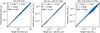Fig. 1

Performance of three surrogate models based on the comparison of the predicted and actual values of the testing set. The insert values show the best regression (ordinary least squares), the Pearson correlation coefficient R², and the RMS of the differences between each predicted and actual value.

4.2 Performance of the surrogate model

We asses the performance of the surrogate models in terms of the best regression (obtained using ordinary least squares), the Pearson correlation coefficient R², and the RMS of the differences between the predicted and target lifetimes (the square root of the mean square error). These were computed on the testing set (Table 4) that the surrogate model has not seen before. The hyper-parameters and results for all surrogate models that are part of this work are presented in Table 5. For three of them, we also show correlation plots in Fig. 1. In all cases, the fitting procedure was performed on the logarithm (base 10) of the values, and so all the reported performances are given in these units.

Concerning the different surrogate models, the ones for the disc lifetimes and for the stellar accretion rates provide the best performance. The ones that are based on the dust disc, namely masses and radii, show a lower performance, especially at 2 Myr. We note that these values are for each single prediction; they represent the level of additional uncertainty for the parameter studies (Sect. 4.3 and Appendix A) while for the population studies (Sect. 5) these errors can average out and result in an even better global accuracy.

The neural networks predicting the disc masses, their radii, and stellar accretion rates were fitted only on the discs that had not vanished at the time. This means that they are supported by a lower number of points than the ones predicting the lifetimes. This also implies that these surrogate models are only constrained in the region of the parameter space where lifetimes are larger than the time of the analysis. Thus, in the remainder of this work we only provide disc masses and stellar accretion rates for discs that have not yet dispersed.

4.3 Effects of photoevaporation

We began our investigations using the surrogate model, performing a parameter study of the effects of the photoevaporation prescriptions on disc lifetimes. For this purpose, we generated two maps, one for internal photoevaporation and one for external photoevaporation, which vary the stellar mass and the controlling parameter of each photoevaporation prescription. In each case, the value of the parameter controlling the other photoevaporation prescription was set at the minimum of the studied range in order to avoid cross effects. We assumed typical values of the remaining parameters: disc-to-star gas mass ratio M_G/M_⋆ = 0.1, dust-to-gas ratio ƒ_D/G = 0.0149, power-law index β = 0.9, period at the inner edge P_in = 10 d, characteristic radius r₁ computed according to Eq. (9), viscosity parameter α = 1 × 10⁻³, fragmentation velocity υ_frag = 2 m s⁻¹, planetesimal formation efficiency ɛ = 1 × 10⁻³, and drift efficiency ζ = 1.

4.3.1 Internal photoevaporation

The resulting map for internal photoevaporation is provided in Fig. 2. Here we observe that the surrogate model predicts several sharp transitions of disc lifetime with stellar mass. The most evident are those between 0.2 and 0.3 M_⊙ and between 0.8 and 0.9 M_⊙ where disc lifetime increases. There are other transitions between 0.4 and 0.5 M_⊙ and between 0.6 and 0.7 M_⊙ where disc lifetime decreases, but only for large X-ray luminosities (L_X > 10³⁰ erg s⁻¹). These transitions match the switch from one photoevaporative profile to another, which are marked by the dashed white lines. This indicates that the profile of surface-density loss has a strong effect on disc lifetime and not only the total mass-loss rate, which gradually changes between each stellar mass. Also, the further out the location of the peak of internal photoevaporation (which is for the profiles of 0.3 M_⊙ and 1.0 M_⊙ stars; see top panel of Fig. 7 of Picogna et al. 2021), the longer the disc lifetimes are in general. We find that this effect is due to a larger inner region where material is not evaporated at all and can only be dispersed by viscous accretion. In this case, the observed disc lifetime is set by the dispersal timescale of the inner disc, which is given by the viscous timescale at the outer radius of the inner disc.

As discussed in Sect. 3.5, the X-ray luminosity is correlated with stellar mass. To highlight this, we show in addition the median stellar X-ray luminosity as a function of stellar mass from Güdel et al. (2007) with the green dashed curve. To determine the expected relationship between disc lifetime and stellar mass, one needs to follow this curve rather than a horizontal line on the plot. We see that internal photoevaporation leads to a limited change in disc lifetime with stellar mass. This is because more massive stars lead to stronger mass-loss rates (owing to a corresponding increase in stellar X-ray luminosity), which compensates for the increase in disc mass (as we assume disc mass to be proportional to stellar mass). This is shown by the black line that traces disc lifetimes of 3 Myr (a typical value in observations), which is consistently lower than the median L_X by a factor of a few.

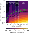Fig. 2

Map of disc lifetimes as a function of stellar mass and X-ray luminosity, which is the main driver of internal photoevaporation, according to the surrogate model described in Sect. 4.2. External photoevaporation was set to its minimum value (F = 1 G₀). Other parameters were selected as M_G/M_⋆ = 0.1, ƒ_D/G = 0.0149, β = 0.9, P_in = 10 d, r₁ according to Eq. (9), α = 1 × 10⁻³, υ_frag = 2 m s⁻¹, ɛ = 1 × 10⁻³, and ζ = 1. The green dashed line represents the dependency of L_X on M_⋆ from Güdel et al. (2007) and the solid black line shows the location of a 3 Myr lifetime (a typical value). The results are discussed in Sect. 4.3.1.

4.3.2 External photoevaporation

The resulting map for external photoevaporation is shown in Fig. 3. Unlike internal photoevaporation, the prescription for external photoevaporation provides for gradual changes of lifetime with stellar mass. However, these changes lead to a larger dependency of disc lifetime on stellar mass than what is expected from internal photoevaporation. This is illustrated by the black line, which tracks a 3 Myr lifetime, as in the map for internal photoevaporation. Its position in terms of ambient UV field strength varies across the entire parameter range studied here, from less that 2 G₀ for M_⋆ = 0.1 M_⊙ to about 4 × 10³ G₀ for M_⋆ = 1 M_⊙; it becomes independent of stellar mass for M_⋆ > 1 M_⊙ and fluxes above ~ 10³ G₀.

While the trend of reduced disc lifetimes in regions with strong ambient UV fields (e.g. Michel et al. 2021) is reproduced, the general behaviour of correlated disc lifetimes with stellar mass for a given ambient UV field strength is problematic for several reasons. First, this general behaviour is inconsistent with observations that suggest disc lifetimes are independent of, or slightly decreasing with, increasing stellar mass (Carpenter et al. 2006; Kennedy & Kenyon 2009; Bayo et al. 2012; Ribas et al. 2015). There are several possibilities to remedy this, although they are unlikely. To obtain a behaviour similar to observations, the mass loss would need to be correlated with stellar mass (Komaki et al. 2021), which in turn would require that the ambient field be correlated with stellar mass. However, the ambient field is usually dominated by the few most massive stars (Adams et al. 2006), which means that it depends more on the cluster as a whole than on the mass of the star in question. Another avenue is that disc masses scale to a lesser extent with stellar mass than assumed here. However, this would not yield the expected behaviour of stellar accretion rates with stellar masses (e.g. Hartmann et al. 2016; Alcalá et al. 2017; Flaischlen et al. 2021). We find that the FRIED grid prescription that we use in this work produces incompatible results that show at most a dependence of the disc lifetime on stellar mass. The second concern is that further lifetime analyses will be strongly affected by the selection of the stellar masses, in contrast to internal photoevaporation where this dependency is weaker.

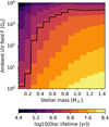Fig. 3

Map of disc lifetime as functions of stellar mass and ambient UV field strength, this latter being the main driver of external photoevaporation according to the surrogate model described in Sect. 4.2. Internal photoevaporation is set to its minimum value (L_X = 1 × 10²⁸erg s⁻¹). Other parameters were selected as M_G/M_⋆ = 0.1, ƒ_D/G = 0.0149, β = 0.9, P_in = 10 d, r₁ according to Eq. (9), α = 1 × 10⁻³, υ_frag = 2 m s⁻¹, ℰ = 1 × 10⁻³, and ζ = 1. The solid black line shows the location of a 3 Myr lifetime (a typical value). The results are discussed in Sect. 4.3.2.

4.4 Parameter sensitivity

The sensitivity of disc lifetimes, disc masses, and stellar accretion rates at 2 Myr is studied in detail in Appendix A. These results can be summarised as follows: all the outcomes are insensitive to the power-law index β and the inner edge of the gas disc r_in. The characteristic radius r₁ and viscosity α control the viscous timescale of the disc, and therefore the stellar accretion rate. Disc lifetimes and observed dust masses are more strongly affected by the viscosity α than by the characteristic radius r₁.

The twopop model parameters only affect the observed dust masses. Observed dust masses are less affected by the dust-to-gas ratio ƒ_D/G than by the initial mass of the gas disc M_G, except for discs close to dispersal. The fragmentation velocity υ_frag and the drift efficiency strongly affect the observed dust masses, but only for υ_frag ≳ 200 cm s⁻¹, while the planetesimal formation efficiency ɛ only has a limited effect for values close to the maximum we study, namely of 0.1.

These results narrow down the parameter space that we explore in the remainder of this work. First, we keep the values of the power-law index β and the inner edge of the gas disc r_in as described in Sect. 3, because they are of negligible importance. We then only use the initial mass of the gas disc M_G to control disc masses, not the dust-to-gas ratio ƒ_D/G; as the latter is in most cases of lower importance and well constrained by observations. Also, we keep the planetesimal formation efficiency to the minimum value of ɛ = 1 × 10⁻³, the fragmentation velocity to υ_frag = 200 cm s⁻¹, and the drift efficiency to ζ = 1.

5 Disc populations

We now compare synthetic disc populations with observations. For this, we proceed as follows: we draw 10,000 random discs whose initial conditions follow given distributions. The outcomes of each disc are obtained by means of the different surrogate models. For the analysis, we first compare the cumulative distribution of disc lifetimes so that it can be compared to the fraction of stars that have a protoplanetary disc for stellar clusters with different ages, as in Haisch et al. (2001). The second analysis is to compare observed disc masses and stellar accretion rates with the data of Manara et al. (2019). Here, we use the data at 2Myr. Further, we only use discs whose lifetime, as determined by the surrogate model from the previous analysis, is larger than the time of analysis in order to avoid being in the region where the surrogate model is not supported by any underlying data.

5.1 Canonical

To determine if all the processes that are predicted from theory are able to reproduce disc observations, we compute a population of discs whose properties are as close as possible to observations from early discs. The only parameter that has some freedom is α. Here, we selected to draw log₁₀ (α) with a uniform probability of between −3.5 and −3. This was decided as a compromise between disc lifetime and stellar accretion rate, as we discuss below. For the other parameters, their distributions were selected as described in the discussion of Sect. 3; for convenience, these are summarised in Table 6.

The resulting distribution of disc lifetimes is shown with the blue curve in Fig. 4. It becomes immediately apparent that the synthetic lifetimes are too short overall in comparison with observed discs. The median lifetime of the synthetic discs is 0.42 Myr. Disc lifetime depends on the assumed distribution of α, which we chose such that it results in the largest stellar accretion rates at 2 Myr. A histogram of stellar accretion rate versus observed dust mass for the observed discs in the Lupus and Chamaeleon I star-forming regions is shown in the top-left panel of Fig. 5. Only the synthetic discs that live beyond 2 Myr contribute to this histogram. The few remaining discs have low masses, as the discs are close to being dissipated. Using larger values of α, for instance between roughly 10^–3 and 10^–2 as was proposed by Mulders et al. (2017), would have resulted in even shorter disc lifetimes. This means that there would have been no discs that would live long enough to produce stellar accretion at 2 Myr. Conversely, selecting a distribution of α with even lower values would allow disc lifetimes to be matched by observations, but this would result in even lower stellar accretion rates, which would be in tension with the results of Dullemond et al. (2018), who concluded that α ≥ 1 × 10^–4 from the sizes of disc substructures.

The discrepancy between our modelled lifetimes and observations arises from the strong mass-loss rates predicted for internal and external photoevaporation, as we discuss in Sect. 6. As disc lifetime depends on stellar mass (especially for external photoevaporation; Sect. 4.3), this analysis is affected by the assumed stellar mass distribution. Had we selected larger stellar masses, the lifetimes would better match observations. However, selecting stellar masses of around 1Μ_⊙, which would lead to a fairly good match including both photoevaporation prescriptions, is not representative of the star-forming regions that we are comparing to (Sect. 3.1).

Table 6

Random distributions for the canonical population.

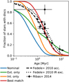Fig. 4

Cumulative distribution of disc lifetimes for a population with canonical parameter distribution (see text). Two exponential decays following Fedele et al. (2010) with a characteristic time of 2.3 Myr (accretion) and 3 Myr (infrared excess) and the results of Ribas et al. (2014) are shown as well.

5.2 Effect of photoevaporation on disc populations

The mismatch in disc lifetimes and disc masses that we obtained is in contrast with other studies, such as that of Mulders et al. (2017), who did not include photoevaporation, Kunitomo et al. (2020), who included only internal photoevaporation, and Weder et al. (2023), who used an EUV-only internal photoevaporation prescription with much lowermass-loss rates. Further, as already discussed, photoevaporation leads to considerable shortening of disc lifetimes (Sect. 4.3). Therefore, here we investigate how the photoevaporation prescriptions affect the evolution of disc populations and determine whether they are responsible for the mismatch. To this end, we created two additional populations, each time neglecting one of the photoevaporation process by taken the corresponding controlling parameter to the minimum value. For the population with internal photoevaporation only, the ambient flux has been set to F = 1G₀, which corresponds to Ṁ = 1 × 10^–15 Μ_⊙ yr^–1 (Sect. 2.1.2). The results are shown as ‘Int. only’ in Figs. 4 and 5. For the population with external photoevaporation only, we set L_x = 10²⁸ erg s^–1, the results of which are shown as ‘Ext. only’ in the same figures.

In each population, the disc lifetimes strongly increase compared to the canonical case. However, the distributions are different: internal photoevaporation leads to a relatively narrow distribution around 2–3 Myr, while with external photoevapora-tion disc lifetimes are more spread out, including very short-lived discs. This leads to more discs being shown in the accretion versus mass diagram.

The population with only external photoevaporation has low disc masses combined with a narrow range of stellar accretion between 10^–10 and 10^–9 Μ_⊙ yr^–1. This is because the mass loss occurs in the outer disc, which reduces its size, limiting the area from which the dust emits (as dust is also lost where there is no longer gas present). At the same time, the mass-accretion rate is weakly affected by the mass loss in the outer disc; again because external photoevaporation affects only the outer disc.

Conversely, using internal photoevaporation leads to a larger spread in stellar accretion rate. As internal photoevaporation removes material relatively close to the star, it competes with stellar accretion to some extent (Somigliana et al. 2020). This, coupled with the spread of X-ray luminosities, leads to a spread in accretion rate (Owen et al. 2011). Thus, internal photoevap-oration is needed to reproduce the observed spread in stellar accretion rate (Manara et al. 2016b; Testi et al. 2022). We further note that neither population is able to reproduce the discs with an accretion rate larger than 10^–8 Μ_⊙ yr^–1.

In addition, internal photoevaporation leaves discs with an inner cavity that have low accretion rates but where the outer disc is out of reach of internal photoevaporation and therefore takes a long time to dissipate; these are what Owen et al. (2011) refer to as relic discs. It is possible to avoid this situation to a large extent by having more compact discs initially, which leave nearly all of their mass within reach of internal photoevaporation.

We conclude that previous studies managed to reproduce disc lifetimes because they used only one photoevaporation mechanism as the main loss mechanism. However, when both are accounted for, the combined mass-loss rate is so large that discs are very short lived. We discuss the implications of this and possible remedies in Sect. 6.

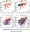Fig. 5

Histogram for stellar accretion rate vs. disc mass at 2Myr and the same synthetic disc populations shown in Fig. 4. The observed data from the Lupus (in red) and Chamaeleon I (orange) star forming regions from Manara et al. (2019) are shown for comparison. Two disc dispersal timescales τ = Ṁ_G/M_G of 1 Myr and 10 Myr (assuming that the gas disc mass M_G is 100 times the observed dust mass) and the best fit to the data from Manara et al. (2016b) are shown as well.

5.3 Towards a best match

Despite all the differences between models and observations highlighted so far, we now try to find a set of initial conditions that is able to better match disc evolution characteristics. To this end, we investigate how the initial conditions can be modified from our canonical values provided in Table 6.

The initial disc-to-star mass ratios were taken from Tychoniec et al. (2018) and Tobin et al. (2020) assuming they were measured on stars of $M_{⋆}^{ref} = 1 M_{⊙}$ $M_ \star ^{{\rm{ref}}} = 1{M_ \odot }$ . However, this assumption is inconsistent with the stellar mass distribution we selected, which has a median value of M_⋆ = 0.35 M_⊙ (Sect. 3.1). Were we to select a lower reference stellar mass, such as $M_{⋆}^{ref} = 0.33 M_{⊙}$ $M_ \star ^{{\rm{ref}}} = 0.33{M_ \odot }$ , this would increase the disc masses. At the same time, selecting a reference stellar mass that is similar to the median value from our initial conditions results in an agreement between the disc masses in observations and our initial conditions, as shown with the dashed black and red lines in Fig. 6, respectively. In addition, to account for observational biases, we also want to check the observed dust masses after a short evolution time of 1 × 10⁵ yr, which we provide with the solid lines in Fig. 6. The results show that the discs in the nominal populations have low masses compared to the non-multiple discs measured by Tobin et al. (2020), while a population with more massive initial discs has slightly larger masses. Thus, the larger initial disc masses lead to a reasonable match with observations as a whole.

We point out that the disc-to-star mass ratio in the population with $M_{⋆}^{ref} = 0.33 M_{⊙}$ $M_ \star ^{{\rm{ref}}} = 0.33{M_ \odot }$ is about twice (2.1 times) that of Emsenhuber et al. (2021b) and Burn et al. (2021), rather than a factor three as one might assume from the change of $M_{⋆}^{ref}$ $M_ \star ^{{\rm{ref}}}$ from 1M_⊙ to 0.33 M_⊙. This is due to an inconsistency in the selection of the disc masses in the previous work: there, the gas masses were taken as a Monte Carlo variable that were converted from dust observations using a dust-to-gas ratio of 1%. However, the initial mass of solids in the model was recomputed from the gas mass using the same distribution as in this work (Sect. 3.4), which has a median value of 1.42% (f_d/g,⊙ = 1.49% with [Fe/H] = –0.02). In contrast, we use the solid disc mass as a Monte Carlo variable here.

Another possibility is that early protoplanetary discs are not as extended as what is suggested by the findings of Tobin et al. (2020). More compact discs are less susceptible to external photoevaporation, as there is less surface exposed to ambient radiation and they are more tightly bound to the star. At the same time, a more compact disc means that more material is concentrated in the region where internal photoevaporation is most efficient, which allows the stellar accretion rate to remain larger. Magnetohydrodynamics models of protoplanetary disc formation by Hennebelle et al. (2016), Lebreuilly et al. (2021), and Lee et al. (2021) could favour such a possibility.

Finally, nearby star-forming regions have low masses, which results in a low ambient UV field strength F ; for instance, the value in Lupus is F ≈ 4G₀ (Cleeves et al. 2016). Our nominal distribution of ambient UV fields overestimates mass losses due to external photoevaporation. Therefore, we set F = 1G₀, which results in negligible mass losses due to external photoevapora-tion (Ṁ = 1 × 10^–15 M_⊙ yr^–1) and only internal photoevaporation remains. Using internal photoevaporation confers the further advantage that a wider range of stellar accretion rates is obtained.

Below, we investigate whether more massive and compact discs are able to improve the match with observations. The effects of the parameters mentioned above are discussed in Appendix B. From these, we find that the following modifications to the initial conditions given in Table 6 are best able to reproduce disc lifetimes and the accretion rate–mass relationship:

A decrease in the reference stellar mass to $M_{⋆}^{ref} = 0.33 M_{⊙}$ $M_ \star ^{{\rm{ref}}} = 0.33{M_ \odot }$ , which corresponds to an increase in the disc mass by a factor of three compared to the nominal population; – r₁ = 2/3 × 70 au (M_d/100 M_⊕)^0.25, a factor 2/3 compared to Eq. (9); and
only using internal photoevaporation (F = 1G₀).

The population using these distributions is shown as ‘Best match’ in Figs. 4 and 5.

While the overall stellar mass distribution we chose is representative of the observed stars, our visual optimisation approach to reproducing the observed disc masses and accretion rates is independent of the exact stellar mass dependency of the observables. We will improve on this with a Bayesian framework in Paper III to optimise the initial parameters when reproducing a set of observations in four-dimensional space made up of stellar mass, disc mass, disc radius, and accretion rate.

Compared to the population with only internal photoevap-oration (the other population that is closest in terms of initial conditions), we can see several differences. First, the larger disc masses result in an increased median lifetime. About 2.2% of the discs have a lifetime of greater than 10 Myr, representing a 100-fold increase. Then, the combination of larger initial disc mass and smaller extent results in a certain number of cases with a stellar accretion rate of higher than 10^–8 M_⊙ yr^–1, which was not previously seen. The smaller extent of the disc also causes less discs to be relics (towards the bottom of Fig. 5). Here, the highest concentration of discs is found near the best-fit value of Manara et al. (2016b, the pink dashed line in Fig. 5) with a similar number on either side. We are still failing to reproduce the discs with the large accretion rates. However, part of these discs with large accretion rates could be due to binaries (Zagaria et al. 2022), which we do not model. To corroborate this, the largest stellar accretion rates are biased to larger-mass stars (the mean stellar mass for systems with a stellar accretion rate higher than 3 × 10^–9 M_⊙ yr^–1 is 0.74 M_⊙ versus 0.43 M_⊙ for the general population), which at the same time are more likely to be in binary systems (e.g. Duchêne & Kraus 2013). The mismatch should therefore not be the source of significant concern. We find that this combination of parameters is able to reproduce the disc mass–accretion rate relationship and provide a reasonable match to most observations.

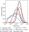Fig. 6

Kernel density estimate for two populations from Figs. 4 and 5, both for their initial conditions (dashed lines) and retrieved disc masses at 100 kyr (solid lines). The initial mass distribution of the best-match population with $M_{⋆}^{ref} = 0.33 M_{⊙}$ $M_ \star ^{{\rm{ref}}} = 0.33{M_ \odot }$ (in red) is consistent with the fit by Emsenhuber et al. (2021b) to the data of Tychoniec et al. (2018), which are shown as the dashed black line, while the retrieved masses at 100 kyr are compatible with the non-multiple discs of Tobin et al. (2020).

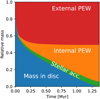Fig. 7

Evolution of the relative gas mass: in the disc (blue), accreted onto the star (green), and lost by internal (orange) or external (red) photoevaporation until disc dispersal at 1.38 Myr. This represents a typical disc, with M_⋆ = 0.5 M_⊙, M_G/M_⋆ = 0.1, β = 0.9, R_in = 0.1 au, r₁ = 87.8 au, α = 1 × 10^–3, L_X = 7.02 × 10²⁹ ergs^–1, and F = 10 G₀. The parameters for the solid disc are irrelevant, as this shows only the gas component, except that we used f_D/G = 0.0149 to compute the solid mass needed to set the characteristic radius r₁.

6 Discussion

It is difficult to reconcile the results of our synthetic disc populations with observations. We find that it is particularly hard to obtain discs with characteristic lifetimes of 2–3 Myr according to Mamajek (2009) or Fedele et al. (2010), and even less lifetimes of 5 to 10 Myr following Pfalzner et al. (2022). Here, we assumed that the initial mass is constrained by the dust-mass measurements of Tychoniec et al. (2018, M_D/M_⋆ ~ 10^–3), and dust-to-gas ratios similar to the solar initial abundance, namely f_d/g = 1.49% (Lodders 2003), combined with the predictions of internal and external photoevaporation models. To illustrate this issue, in Fig. 7 we provide the evolution of the gas mass still present in the disc and removed by the processes modelled here. Here we choose typical values for the initial conditions, with a star of mass M_⋆ = 0.5 M_⊙, a gas disc with a mass of M_G/M_⋆ = 0.1, a power-law index of β = 0.9, an inner radius of r_in = 0.1 au, and a characteristic radius of r₁ = 87.8 au, which was computed from Eq. (9) assuming a dust-to-gas ratio of f_D/G = 0.0149. The ambient UV field strength F = 10 G₀ was set at the lower boundary of the computed grid while the X-ray luminosity L_X = 7.02 × 10²⁹ erg s^–1 follows the best fit of the XEST survey (Güdel et al. 2007, Table 2) for the given stellar mass.

Figure 7 shows that photoevaporation (both internal and external) is responsible for the loss of nearly all the gas; only 6% of the gas is accreted onto the star. The final disc lifetime of 1.38 Myr is short compared to the characteristic lifetimes from observations. We therefore have a problem with the mass budget, which could be resolved by (i) larger initial disc masses, (ii) mass replenishment after disc formation, or (iii) lower mass-loss rates by photoevaporation.

Stellar accretion already plays a minor role in the mass budget and cannot be reduced further, in order to remain consistent with observed stellar accretion rates. However, radial mass transport could be the result of magnetically driven disc winds (Suzuki & Inutsuka 2009; Suzuki et al. 2010) rather than pure viscous dissipation as we assumed here. This would add another mass-loss channel, which would further exacerbate the problem (though it could shield stellar radiation, as discussed below).

We experiment with larger initial disc masses in this work. However, even with gas masses on the order of 10% of the stellar mass, disc lifetimes are not sufficiently long. Therefore, increasing the masses even more would be required, but this increase would bring another series of problems. For one, such large discs are likely gravitationally unstable and produce spiral density waves. Second, such large discs would lead to strong gas-driven migration, which hinders planet formation (Nayakshin et al. 2022). Also, discs around 10Myr-old stars HD 163296 and TW Hya have at least 10% of the stellar mass (Powell et al. 2019) and it is unclear what their initial mass would have been for them to remain so large at their age. We therefore do not find that massive initial discs would be able to solve the conundrum.

Discs do not form instantly. Rather, they grow from gas falling from the envelope. This allows for disc masses to increase during the early stages of disc evolution, which is at odds with the models described here. Modelling the infall stage would allow us to have longer-lived discs without them being very massive early on. Accretion can persist for several million years (Throop & Bally 2008), providing replenishment even at late times. The complex morphology of the gas disc around RU Lup (a ~0.5Myr old star) could be an outcome of this process (Huang et al. 2020). The long-lived discs could also be second-generation discs, formed following accretion from the molecular cloud (Kuffmeier et al. 2020) or the disruption of a planet (Nayakshin et al. 2020). While none of these individual processes are sufficient to explain the presence of massive discs, they should still be explored if they can explain certain characteristics of the overall disc population.

Finally, the photoevaporation rates used here could be overestimated. Lower mass-loss rates would increase the disc lifetimes and masses at later times. An argument in favour of this hypothesis is that young discs can be shielded from the radiation of both their host and nearby stars. The launching of magnetically driven disc winds occurs inside the location where internal photoevaporation is effective and would thus prevent EUV and X-ray photoevaporation during the early stages of disc evolution (Pascucci et al. 2022). Similarly, early discs are likely embedded, preventing the radiation of nearby stars from reaching the disc. Both effects would reduce the photoevaporation rates during the early stage of disc evolution compared to what we model here.

7 Summary and conclusion

In this work, we investigate whether protoplanetary disc observations can be reconciled with theoretical predictions of processes such as viscous accretion and photoevaporation (both internal and external). We first compute two sets of simulations that we use to fit neural networks (Fig. 1). With these neural networks, we can perform parameter studies and compute the outcomes of synthetic disc populations with limited computational resources.

We first compare how internal and external photoevaporation affect disc lifetime as a function of stellar mass. We find that because of a direct link between stellar mass and X-ray luminosity (e.g. Preibisch et al. 2005; Güdel et al. 2007), which means mass-loss rate due to internal photoevaporation, discs around more massive stars are not significantly longer-lived than those around low-mass stars (Fig. 2). Conversely, external photoevapo-ration leads to a strong positive correlation between disc lifetime and stellar mass (Fig. 3), because gas is more bound for highermass stars. This positive correlation is at odds with observations that find that disc lifetimes are either independent of or anti-correlated with stellar mass (Carpenter et al. 2006; Kennedy & Kenyon 2009; Bayo et al. 2012; Ribas et al. 2015; Pfalzner et al. 2022) and should be investigated in the future.

Turning to protoplanetary disc populations, we find that accounting for both internal and external photoevaporation according to theoretical predictions leads to disc lifetimes (Fig. 4) that are much too short. Discs whose initial mass is 10% of the stellar mass are dispersed in roughly 1 Myr under the combined effects of internal and external photoevaporation (Fig. 7).

Despite the dissimilarities, a reasonably good match to the disc properties of the Lupus and Chaemeleon I low-mass star-forming regions is obtained starting with more massive discs of smaller sizes, and with only internal photoevaporation. This is valid for clusters with low ambient field strengths, such as Lupus (4G₀; Cleeves et al. 2016), where losses due to external photoevaporation are low. The larger masses and smaller sizes are needed to improve the match in stellar accretion rates and observed masses. The corresponding initial conditions and model parameters can be used to study planetary formation in similar environments. A more robust comparison with observations is performed in Paper III.

However, initial disc masses cannot be arbitrarily increased or discs would become gravitationally unstable. Instead, we suggest that future studies should include the modelling of the initial stages of disc formation, including the presence of an envelope. This envelope would allow discs to be replenished after their initial formation and provide shielding from UV radiation from nearby stars. Also, magnetically driven disc winds would shield UV and X-ray radiation from the central star. This would provide a reduction of losses by both internal and external photoevapora-tion. Both effects allow for longer lifetimes and larger masses at later times without the need for extremely large masses at earlier times.

We decided here to use observed dust masses as the main comparison point. However, this is not the only possible avenue. For instance, disc radii could be less susceptible to the degeneracy caused by regions that are optically thick (Pascucci et al. 2022). One likely difficulty would be in accounting for the large disc radii and sustained stellar accretion rate. Already with the comparatively small discs that we find to best match the disc mass–stellar accretion rate relationship, we are not able to reproduce the largest observed accretion rates. Having larger discs would lead to a reduction of the stellar accretion rates for a given disc mass (Fig. B.1); which would lead to a mismatch with observations of stellar accretion rates.

In this work, we assume that the gas discs evolve viscously. However, simulations of disc evolution that account for non-ideal magnetohydrodynamical (MHD) effects find that the magnetorotational instability (MRI), which is the likely mechanism generating the turbulence, is largely suppressed (e.g. Bai & Stone 2013; Lesur et al. 2014). Instead, it has also been proposed that the evolution is driven by magnetically driven disc winds (Suzuki & Inutsuka 2009). Magnetically driven disc wind prescriptions, such as those of Suzuki et al. (2016) or Tabone et al. (2022), include several model possibilities, which can be narrowed down by performing a similar comparison to that presented here (Weder et al. 2023). Once such a model is properly coupled with internal photoevaporation to account for shielding, a similar study to that presented here is possible.

Acknowledgements

The authors thank Christian Rab, Ilaria Pascucci, Susanne Pfalzner, and Aashish Gupta for fruitful discussions. We also thank the anonymous reviewer, whose comments and suggestions greatly helped to improve the manuscript’s quality. This work was funded by the Deutsche Forschungsgemeinschaft (DFG, German Research Foundation) – 362051796. This research was supported by the Excellence Cluster ORIGINS which is funded by the Deutsche Forschungsgemeinschaft (DFG, German Research Foundation) under Germany’s Excelence Strategy – EXC-2094-390783311. The plots shown in this work were generated using matplotlib (Hunter 2007).

Appendix A Parameter study

The surrogate models allow us to study the effects of the different parameters, as shown for stellar mass and photoevaporation in Sect. 4.3. Here, we expand the study to other parameters. The parameters that are not varied are selected as in Sect. 4.3, except for the photoevaporation-related parameters, which are set as L_x = 1 × 10²⁹ergs^–1 and F = 10 G₀ to provide lifetimes that are globally in line with the observations.

We study in Fig. A.1 the effects of the parameters of the gas disc model. The top row shows the outcomes as functions of the power-law index of the initial profile β and the inner edge r_in. These two parameters have very little effect on the final lifetimes, as all values lie within about 0.1 dex, corresponding to a maximum relative difference of 26%. The same applies to disc masses and stellar accretion rates. Thus, the choice of these parameters has negligible effects on the final properties and we do not discuss these parameters further in this work.

The bottom row of Fig. A.1 shows the effect of the viscosity parameter α and the disc’s characteristic radius r₁. The characteristic radius has limited effect on the disc lifetimes while α, which affects the whole viscous evolution, has an important effect. However, both parameters affect the stellar accretion rate, making it possible to combine these two parameters to set the behaviour of stellar accretion versus lifetime.

Figure A.2 shows the same analysis but for the parameters of the solid disc. As such, only the observed dust masses are shown for each parameter combination. The left panel features the dust-to-gas ratio f_D/G and the disc’s gas mass M_G/M_⋆. The results show that the dust-to-gas ratio is only important to control the observed disc masses for discs that are close to dispersal (towards the left of the panel) while it has a lower effect on more massive discs. The centre panel shows two of the twopop model parameters, planetesimal formation efficiency and dust-to-gas ratio. The panel shows that the planetesimal formation efficiency parameter ε is of lower importance than the initial dust mass (which is controlled by the dust-to-gas ratio f_D/G) for the observed disc masses. The right panels show two other twopop model parameters, the drift efficiency ζ and the fragmentation velocity υ_frag. Here we see that fragmentation velocities υ_frag ≳ 300 cm s^–1 lead to lower disc masses because drift becomes efficient. This effect can be counterbalanced by reducing the drift efficiency ζ. However, for a value of υ_frag = 200 cms^–1, the drift efficiency has a small effect on the observed disc masses, which indicate that drift is already inefficient.

One might expect observed dust masses to be affected equally by the two parameters shown in the left panel (as the initial solid mass is the product of the dust-to-gas ratio and the gas mass M_G). However, our results indicate that the initial gas mass has a greater effect than the dust-to-gas ratio.

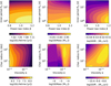Fig. A.1

Gas disc lifetime (left), observed dust masses at 2 Myr (centre), and stellar accretion rates at 2 Myr (right) as functions of the power-law index of the initial profile β and the inner edge r_in (top) or viscosity parameter α and characteristic radius r₁ (bottom) In the bottom row, the white region is where disc lifetimes are less than 2 Myr and the values cannot be constrained by the model.

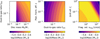Fig. A.2

Observed mass at 2 Myr as function of the parameters of the twopop model: gas-disc mass and dust-to-gas ratio (left), planetesimal formation efficiency and fragmentation velocity (centre), and drift efficiency and fragmentation velocity (right).

Appendix B Best parameters for population

To show how the different model parameters affect the mass-accretion rate relationship and how we came to select the best model parameters, in Fig. B.1 we provide several 2D histograms similar to those shown in Fig. 5, but varying one parameter at a time. These were generated with the parameters of the ‘best match’ population, except for the parameter being varied.

The first row of the figure shows the effect of varying the disc mass (both gas and solids). We see that an increase in the initial mass is recovered in the observed mass after 2 Myr of evolution. In addition, the stellar accretion rate is correlated with the disc mass similarly to the best fit of Manara et al. (2016b). The initial disc mass can therefore be used to set observed masses and an increase from the canonical value is required to obtain disc masses consistent with observations. However, this parameter cannot be used to control the behaviour of the stellar accretion rates for given disc masses.

The second row of the same figure shows the effect of reducing the disc’s characteristic radius by a certain factor. Smaller discs will result in increased stellar accretion rates for a given disc mass while also reducing the occurrence of non-accreting discs (the ones at the bottom of the plot). In addition, smaller discs will also tend to have greater disc lifetimes because they are less affected by photoevaporation. Discs that follow the relationship of Tobin et al. (2020) are found to have overly low accretion rates for their masses, while when reduced by a factor two, stellar accretion rates are now too high. The best-fit parameter is therefore between these two.

Then, the third row shows the effect of the α viscosity parameter. The synthetic populations shown here show less spread due to the use of a fixed value of α, whereas the ones above have the individual values selected from a distribution that goes from 10^–3.5 to 10^–3.0. The results are in line with the discussion in Sect. 5.1: low values of α result in low accretion rates with a large amount of remaining discs, while large values result in a small number of discs with excessive stellar accretion rates. Therefore, while large values of α could be used to have large accretion rates, they would also require a corresponding increase in the initial disc masses to maintain the expected lifetime distribution. We find that values around α = 1 × 10^–3 provide a reasonable match to disc lifetimes and stellar accretion rates. In addition, we also note that there is an increase in the observed dust masses along with α, which is related to the extent of the solid disc. With large α, the grains do not grow as much as with lower α, and as a consequence do not drift as fast. Hence, the dust emits from a larger area, which is then reflected in the emitted flux and the observed mass. However, this effect only lasts until the dispersal of the gas disc.

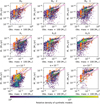Fig. B.1

2D histograms for stellar accretion rate versus disc mass at 2 Myr, showing the effects of the different parameters, as given above each panel. The top row shows the effect of increasing the initial disc mass M_D. The middle row shows the effect of reducing the disc characteristic radius r₁. The bottom row shows the effect of the disc viscosity parameter α. The observed data from the Lupus (in red) and Chamaeleon I (orange) star-forming regions from Manara et al. (2019) are shown for comparison.

References

Adams, F. C., Proszkow, E. M., Fatuzzo, M., & Myers, P. C. 2006, ApJ, 641, 504 [NASA ADS] [CrossRef] [Google Scholar]
Alcalá, J. M., Natta, A., Manara, C. F., et al. 2014, A&A, 561, A2 [NASA ADS] [CrossRef] [EDP Sciences] [Google Scholar]
Alcalá, J. M., Manara, C. F., Natta, A., et al. 2017, A&A, 600, A20 [NASA ADS] [CrossRef] [EDP Sciences] [Google Scholar]
Alexander, R. D., Clarke, C. J., & Pringle, J. E. 2004, MNRAS, 354, 71 [NASA ADS] [CrossRef] [Google Scholar]
Alibert, Y., Mordasini, C., & Benz, W. 2004, A&A, 417, L25 [NASA ADS] [CrossRef] [EDP Sciences] [Google Scholar]
Alibert, Y., Mordasini, C., Benz, W., & Winisdoerffer, C. 2005, A&A, 434, 343 [NASA ADS] [CrossRef] [EDP Sciences] [Google Scholar]
Andrews, S. M., Wilner, D. J., Hughes, A. M., Qi, C., & Dullemond, C. P. 2009, ApJ, 700, 1502 [CrossRef] [Google Scholar]
Andrews, S. M., Wilner, D. J., Hughes, A. M., Qi, C., & Dullemond, C. P. 2010, ApJ, 723, 1241 [Google Scholar]
Andrews, S. M., Huang, J., Pérez, L. M., et al. 2018a, ApJ, 869, L41 [NASA ADS] [CrossRef] [Google Scholar]
Andrews, S. M., Terrell, M., Tripathi, A., et al. 2018b, ApJ, 865, 157 [Google Scholar]
Ansdell, M., Williams, J. P., van der Marel, N., et al. 2016, ApJ, 828, 46 [Google Scholar]
Ansdell, M., Williams, J. P., Manara, C. F., et al. 2017, AJ, 153, 240 [Google Scholar]
Bai, X.-N., & Stone, J. M. 2013, ApJ, 769, 76 [Google Scholar]
Baraffe, I., Chabrier, G., Allard, F., & Hauschildt, P. H. 1998, A&A, 337, 403 [Google Scholar]
Baraffe, I., Homeier, D., Allard, F., & Chabrier, G. 2015, A&A, 577, A42 [NASA ADS] [CrossRef] [EDP Sciences] [Google Scholar]
Bayo, A., Barrado, D., Huélamo, N., et al. 2012, A&A, 547, A80 [NASA ADS] [CrossRef] [EDP Sciences] [Google Scholar]
Beckwith, S. V. W., & Sargent, A. I. 1996, Nature, 383, 139 [NASA ADS] [CrossRef] [Google Scholar]
Birnstiel, T., Dullemond, C. P., & Brauer, F. 2010, A&A, 513, A79 [NASA ADS] [CrossRef] [EDP Sciences] [Google Scholar]
Birnstiel, T., Klahr, H., & Ercolano, B. 2012, A&A, 539, A148 [NASA ADS] [CrossRef] [EDP Sciences] [Google Scholar]
Birnstiel, T., Dullemond, C. P., Zhu, Z., et al. 2018, ApJ, 869, L45 [CrossRef] [Google Scholar]
Burn, R., Schlecker, M., Mordasini, C., et al. 2021, A&A, 656, A72 [NASA ADS] [CrossRef] [EDP Sciences] [Google Scholar]
Burn, R., Emsenhuber, A., Weder, J., et al. 2022, A&A, 666, A73 [NASA ADS] [CrossRef] [EDP Sciences] [Google Scholar]
Burn, R., Emsenhuber, A., Melon Fuksman, J. D., et al. 2023, A&A, submitted (Paper III) [Google Scholar]
Byrd, R. H., Lu, P., Nocedal, J., & Zhu, C. 1995, SIAM J. Sci. Comput., 16, 1190 [Google Scholar]
Cambioni, S., Asphaug, E., Emsenhuber, A., et al. 2019a, ApJ, 875, 40 [NASA ADS] [CrossRef] [Google Scholar]
Cambioni, S., Delbo, M., Ryan, A. J., Furfaro, R., & Asphaug, E. 2019b, Icarus, 325, 16 [NASA ADS] [CrossRef] [Google Scholar]
Cambioni, S., Jacobson, S. A., Emsenhuber, A., et al. 2021, PSJ, 2, 93 [NASA ADS] [CrossRef] [Google Scholar]
Carpenter, J. M., Mamajek, E. E., Hillenbrand, L. A., & Meyer, M. R. 2006, ApJ, 651, L49 [NASA ADS] [CrossRef] [Google Scholar]
Chabrier, G. 2003, PASP, 115, 763 [Google Scholar]
Clarke, C. J., Gendrin, A., & Sotomayor, M. 2001, MNRAS, 328, 485 [NASA ADS] [CrossRef] [Google Scholar]
Cleeves, L. I., Öberg, K. I., Wilner, D. J., et al. 2016, ApJ, 832, 110 [Google Scholar]
Da Rio, N., Robberto, M., Hillenbrand, L. A., Henning, T., & Stassun, K. G. 2012, ApJ, 748, 14 [Google Scholar]
Dittrich, K., Klahr, H., & Johansen, A. 2013, ApJ, 763, 117 [NASA ADS] [CrossRef] [Google Scholar]
Drążkowska, J., & Alibert, Y. 2017, A&A, 608, A92 [Google Scholar]
Duchêne, G., & Kraus, A. 2013, ARA&A, 51, 269 [Google Scholar]
Dullemond, C. P., Birnstiel, T., Huang, J., et al. 2018, ApJ, 869, L46 [NASA ADS] [CrossRef] [Google Scholar]
Emsenhuber, A., Cambioni, S., Asphaug, E., et al. 2020, ApJ, 891, 6 [NASA ADS] [CrossRef] [Google Scholar]
Emsenhuber, A., Mordasini, C., Burn, R., et al. 2021a, A&A, 656, A69 [NASA ADS] [CrossRef] [EDP Sciences] [Google Scholar]
Emsenhuber, A., Mordasini, C., Burn, R., et al. 2021b, A&A, 656, A70 [NASA ADS] [CrossRef] [EDP Sciences] [Google Scholar]
Ercolano, B., Drake, J. J., Raymond, J. C., & Clarke, C. C. 2008, ApJ, 688, 398 [Google Scholar]
Ercolano, B., Clarke, C. J., & Drake, J. J. 2009, ApJ, 699, 1639 [Google Scholar]
Ercolano, B., Clarke, C. J., & Hall, A. C. 2011, MNRAS, 410, 671 [Google Scholar]
Ercolano, B., Koepferl, C., Owen, J., & Robitaille, T. 2015, MNRAS, 452, 3689 [NASA ADS] [CrossRef] [Google Scholar]
Ercolano, B., Picogna, G., Monsch, K., Drake, J. J., & Preibisch, T. 2021, MNRAS, 508, 1675 [NASA ADS] [CrossRef] [Google Scholar]
Facchini, S., Clarke, C. J., & Bisbas, T. G. 2016, MNRAS, 457, 3593 [NASA ADS] [CrossRef] [Google Scholar]
Favata, F., & Micela, G. 2003, Space Sci. Rev., 108, 577 [NASA ADS] [CrossRef] [Google Scholar]
Fedele, D., van den Ancker, M. E., Henning, T., Jayawardhana, R., & Oliveira, J. M. 2010, A&A, 510, A72 [NASA ADS] [CrossRef] [EDP Sciences] [Google Scholar]
Feigelson, E. D., & Montmerle, T. 1999, ARA&A, 37, 363 [Google Scholar]
Flaischlen, S., Preibisch, T., Manara, C. F., & Ercolano, B. 2021, A&A, 648, A121 [NASA ADS] [CrossRef] [EDP Sciences] [Google Scholar]
Fortier, A., Alibert, Y., Carron, F., Benz, W., & Dittkrist, K. M. 2013, A&A, 549, A4 [NASA ADS] [CrossRef] [EDP Sciences] [Google Scholar]
Franz, R., Picogna, G., Ercolano, B., & Birnstiel, T. 2020, A&A, 635, A53 [EDP Sciences] [Google Scholar]
Gárate, M., Birnstiel, T., Drążkowska, J., & Stammler, S. M. 2020, A&A, 635, A149 [NASA ADS] [CrossRef] [EDP Sciences] [Google Scholar]
Gáspár, A., Rieke, G. H., & Ballering, N. 2016, ApJ, 826, 171 [Google Scholar]
Getman, K. V., Flaccomio, E., Broos, P. S., et al. 2005, ApJS, 160, 319 [NASA ADS] [CrossRef] [Google Scholar]
Gómez de Castro, A. I. 2009, Ap&SS, 320, 97 [CrossRef] [Google Scholar]
Gorti, U., Dullemond, C. P., & Hollenbach, D. 2009, ApJ, 705, 1237 [Google Scholar]
Güdel, M., Briggs, K. R., Arzner, K., et al. 2007, A&A, 468, 353 [Google Scholar]
Gundlach, B., Schmidt, K. P., Kreuzig, C., et al. 2018, MNRAS, 479, 1273 [NASA ADS] [CrossRef] [Google Scholar]
Habing, H. J. 1968, Bull. Astron. Inst. Netherlands, 19, 421 [Google Scholar]
Haisch, J., Karl, E., Lada, E. A., & Lada, C. J. 2001, ApJ, 553, L153 [NASA ADS] [CrossRef] [Google Scholar]
Hartmann, L., Herczeg, G., & Calvet, N. 2016, ARA&A, 54, 135 [Google Scholar]
Haworth, T. J., Clarke, C. J., Rahman, W., Winter, A. J., & Facchini, S. 2018, MNRAS, 481, 452 [NASA ADS] [CrossRef] [Google Scholar]
Hendler, N., Pascucci, I., Pinilla, P., et al. 2020, ApJ, 895, 126 [Google Scholar]
Hennebelle, P., Commerçon, B., Chabrier, G., & Marchand, P. 2016, ApJ, 830, L8 [Google Scholar]
Hollenbach, D., Johnstone, D., Lizano, S., & Shu, F. 1994, ApJ, 428, 654 [NASA ADS] [CrossRef] [Google Scholar]
Huang, J., Andrews, S. M., Öberg, K. I., et al. 2020, ApJ, 898, 140 [NASA ADS] [CrossRef] [Google Scholar]
Hueso, R., & Guillot, T. 2005, A&A, 442, 703 [NASA ADS] [CrossRef] [EDP Sciences] [Google Scholar]
Hunter, J. D. 2007, Comput. Sci. Eng., 9, 90 [NASA ADS] [CrossRef] [Google Scholar]
Johnstone, C. P., Bartel, M., & Güdel, M. 2021, A&A, 649, A96 [EDP Sciences] [Google Scholar]
Kennedy, G. M., & Kenyon, S. J. 2009, ApJ, 695, 1210 [NASA ADS] [CrossRef] [Google Scholar]
Kimura, S. S., Kunitomo, M., & Takahashi, S. Z. 2016, MNRAS, 461, 2257 [NASA ADS] [CrossRef] [Google Scholar]
Kingma, D. P., & Ba, J. 2014, ArXiv e-prints [arXiv:1412.6980] [Google Scholar]
Koepferl, C. M., Ercolano, B., Dale, J., et al. 2013, MNRAS, 428, 3327 [Google Scholar]
Komaki, A., Nakatani, R., & Yoshida, N. 2021, ApJ, 910, 51 [NASA ADS] [CrossRef] [Google Scholar]
Kraus, A. L., Ireland, M. J., Hillenbrand, L. A., & Martinache, F. 2012, ApJ, 745, 19 [Google Scholar]
Kuffmeier, M., Goicovic, F. G., & Dullemond, C. P. 2020, A&A, 633, A3 [NASA ADS] [CrossRef] [EDP Sciences] [Google Scholar]
Kunitomo, M., Suzuki, T. K., & Inutsuka, S.-I. 2020, MNRAS, 492, 3849 [CrossRef] [Google Scholar]
Kunitomo, M., Ida, S., Takeuchi, T., et al. 2021, ApJ, 909, 109 [NASA ADS] [CrossRef] [Google Scholar]
Lada, C. J., & Lada, E. A. 2003, ARA&A, 41, 57 [Google Scholar]
Lebreuilly, U., Hennebelle, P., Colman, T., et al. 2021, ApJ, 917, L10 [NASA ADS] [CrossRef] [Google Scholar]
Lee, Y.-N., Marchand, P., Liu, Y.-H., & Hennebelle, P. 2021, ApJ, 922, 36 [NASA ADS] [CrossRef] [Google Scholar]
Lenz, C. T., Klahr, H., & Birnstiel, T. 2019, ApJ, 874, 36 [NASA ADS] [CrossRef] [Google Scholar]
Lesur, G., Kunz, M. W., & Fromang, S. 2014, A&A, 566, A56 [NASA ADS] [CrossRef] [EDP Sciences] [Google Scholar]
Lodders, K. 2003, ApJ, 591, 1220 [Google Scholar]
Luhman, K. L. 2000, ApJ, 544, 1044 [NASA ADS] [CrossRef] [Google Scholar]
Lüst, R. 1952, Zeitschrift Naturforschung Teil A, 7, 87 [CrossRef] [Google Scholar]
Lynden-Bell, D., & Pringle, J. E. 1974, MNRAS, 168, 603 [Google Scholar]
Mamajek, E. E. 2009, AIP Conf. Ser., 1158, 3 [Google Scholar]
Manara, C. F., Robberto, M., Da Rio, N., et al. 2012, ApJ, 755, 154 [NASA ADS] [CrossRef] [Google Scholar]
Manara, C. F., Fedele, D., Herczeg, G. J., & Teixeira, P. S. 2016a, A&A, 585, A136 [NASA ADS] [CrossRef] [EDP Sciences] [Google Scholar]
Manara, C. F., Rosotti, G., Testi, L., et al. 2016b, A&A, 591, L3 [NASA ADS] [CrossRef] [EDP Sciences] [Google Scholar]
Manara, C. F., Testi, L., Herczeg, G. J., et al. 2017, A&A, 604, A127 [NASA ADS] [CrossRef] [EDP Sciences] [Google Scholar]
Manara, C. F., Mordasini, C., Testi, L., et al. 2019, A&A, 631, L2 [NASA ADS] [CrossRef] [EDP Sciences] [Google Scholar]
Matsuyama, I., Johnstone, D., & Hartmann, L. 2003, ApJ, 582, 893 [NASA ADS] [CrossRef] [Google Scholar]
McKay, M. D., Beckman, R. J., & Conover, W. J. 1979, Technometrics, 21, 239 [Google Scholar]
Michel, A., van der Marel, N., & Matthews, B. C. 2021, ApJ, 921, 72 [CrossRef] [Google Scholar]
Mordasini, C., Alibert, Y., & Benz, W. 2009, A&A, 501, 1139 [CrossRef] [EDP Sciences] [Google Scholar]
Mulders, G. D., Pascucci, I., Manara, C. F., et al. 2017, ApJ, 847, 31 [NASA ADS] [CrossRef] [Google Scholar]
Murray, N., Chaboyer, B., Arras, P., Hansen, B., & Noyes, R.W. 2001, ApJ, 555, 801 [NASA ADS] [CrossRef] [Google Scholar]
Musiolik, G., & Wurm, G. 2019, ApJ, 873, 58 [NASA ADS] [CrossRef] [Google Scholar]
Nakagawa, Y., Sekiya, M., & Hayashi, C. 1986, Icarus, 67, 375 [Google Scholar]
Nakamoto, T., & Nakagawa, Y. 1994, ApJ, 421, 640 [Google Scholar]
Nayakshin, S., Tsukagoshi, T., Hall, C., et al. 2020, MNRAS, 495, 285 [Google Scholar]
Nayakshin, S., Elbakyan, V., & Rosotti, G. 2022, MNRAS, 512, 6038 [NASA ADS] [CrossRef] [Google Scholar]
Owen, J. E., Ercolano, B., & Clarke, C. J. 2011, MNRAS, 412, 13 [Google Scholar]
Owen, J. E., Clarke, C. J., & Ercolano, B. 2012, MNRAS, 422, 1880 [Google Scholar]
Pascucci, I., Testi, L., Herczeg, G. J., et al. 2016, ApJ, 831, 125 [Google Scholar]
Pascucci, I., Cabrit, S., Edwards, S., et al. 2022, ArXiv e-prints [arXiv:2203.10068] [Google Scholar]
Pedregosa, F., Varoquaux, G., Gramfort, A., et al. 2011, J. Mach. Learn. Res., 12, 2825 [Google Scholar]
Pfalzner, S., Dehghani, S., & Michel, A. 2022, ApJ, 939, L10 [NASA ADS] [CrossRef] [Google Scholar]
Picogna, G., Ercolano, B., Owen, J. E., & Weber, M. L. 2019, MNRAS, 487, 691 [Google Scholar]
Picogna, G., Ercolano, B., & Espaillat, C. C. 2021, MNRAS, 508, 3611 [NASA ADS] [CrossRef] [Google Scholar]
Powell, D., Murray-Clay, R., Pérez, L. M., Schlichting, H. E., & Rosenthal, M. 2019, ApJ, 878, 116 [NASA ADS] [CrossRef] [Google Scholar]
Preibisch, T., Zinnecker, H., & Herbig, G. H. 1996, A&A, 310, 456 [NASA ADS] [Google Scholar]
Preibisch, T., Kim, Y.-C., Favata, F., et al. 2005, ApJS, 160, 401 [NASA ADS] [CrossRef] [Google Scholar]
Qiao, L., Haworth, T. J., Sellek, A. D., & Ali, A. A. 2022, MNRAS, 512, 3788 [NASA ADS] [CrossRef] [Google Scholar]
Ribas, Á., Merín, B., Bouy, H., & Maud, L. T. 2014, A&A, 561, A54 [NASA ADS] [CrossRef] [EDP Sciences] [Google Scholar]
Ribas, Á., Bouy, H., & Merín, B. 2015, A&A, 576, A52 [NASA ADS] [CrossRef] [EDP Sciences] [Google Scholar]
Rosotti, G. P., Clarke, C. J., Manara, C. F., & Facchini, S. 2017, MNRAS, 468, 1631 [NASA ADS] [Google Scholar]
Santos, N. C., Israelian, G., Mayor, M., et al. 2005, A&A, 437, 1127 [NASA ADS] [CrossRef] [EDP Sciences] [Google Scholar]
Sellek, A. D., Booth, R. A., & Clarke, C. J. 2020, MNRAS, 498, 2845 [NASA ADS] [CrossRef] [Google Scholar]
Shakura, N. I., & Sunyaev, R. A. 1973, A&A, 500, 33 [NASA ADS] [Google Scholar]
Somigliana, A., Toci, C., Lodato, G., Rosotti, G., & Manara, C. F. 2020, MNRAS, 492, 1120 [NASA ADS] [CrossRef] [Google Scholar]
Somigliana, A., Toci, C., Rosotti, G., et al. 2022, MNRAS, 514, 5927 [NASA ADS] [CrossRef] [Google Scholar]
Steinpilz, T., Teiser, J., & Wurm, G. 2019, ApJ, 874, 60 [NASA ADS] [CrossRef] [Google Scholar]
Suzuki, T. K., & Inutsuka, S.-I. 2009, ApJ, 691, L49 [Google Scholar]
Suzuki, T. K., Muto, T., & Inutsuka, S.-I. 2010, ApJ, 718, 1289 [NASA ADS] [CrossRef] [Google Scholar]
Suzuki, T. K., Ogihara, M., Morbidelli, A., Crida, A., & Guillot, T. 2016, A&A, 596, A74 [NASA ADS] [CrossRef] [EDP Sciences] [Google Scholar]
Tabone, B., Rosotti, G. P., Cridland, A. J., Armitage, P. J., & Lodato, G. 2022, MNRAS, 512, 2290 [NASA ADS] [CrossRef] [Google Scholar]
Testi, L., Natta, A., Manara, C. F., et al. 2022, A&A, 663, A98 [NASA ADS] [CrossRef] [EDP Sciences] [Google Scholar]
Throop, H. B., & Bally, J. 2008, AJ, 135, 2380 [NASA ADS] [CrossRef] [Google Scholar]
Tobin, J. J., Sheehan, P. D., Megeath, S. T., et al. 2020, ApJ, 890, 130 [CrossRef] [Google Scholar]
Toci, C., Rosotti, G., Lodato, G., Testi, L., & Trapman, L. 2021, MNRAS, 507, 818 [NASA ADS] [CrossRef] [Google Scholar]
Tripathi, A., Andrews, S. M., Birnstiel, T., & Wilner, D. J. 2017, ApJ, 845, 44 [Google Scholar]
Tychoniec, Ł., Tobin, J. J., Karska, A., et al. 2018, ApJS, 238, 19 [Google Scholar]
Tychoniec, Ł., Manara, C. F., Rosotti, G. P., et al. 2020, A&A, 640, A19 [NASA ADS] [CrossRef] [EDP Sciences] [Google Scholar]
van Terwisga, S. E., van Dishoeck, E. F., Mann, R. K., et al. 2020, A&A, 640, A27 [NASA ADS] [CrossRef] [EDP Sciences] [Google Scholar]
Venuti, L., Bouvier, J., Cody, A. M., et al. 2017, A&A, 599, A23 [NASA ADS] [CrossRef] [EDP Sciences] [Google Scholar]
Veras, D., & Armitage, P. J. 2004, MNRAS, 347, 613 [Google Scholar]
Virtanen, P., Gommers, R., Oliphant, T. E., et al. 2020, Nat. Methods, 17, 261 [Google Scholar]
Voelkel, O., Klahr, H., Mordasini, C., Emsenhuber, A., & Lenz, C. 2020, A&A, 642, A75 [NASA ADS] [CrossRef] [EDP Sciences] [Google Scholar]
Weder, J., Mordasini, C., & Emsenhuber, A. 2023, A&A, in press, https://doi.org/10.1051/0004-6361/202243453 [NASA ADS] [CrossRef] [EDP Sciences] [Google Scholar]
Williams, J. P., Cieza, L., Hales, A., et al. 2019, ApJ, 875, L9 [Google Scholar]
Winter, A. J., & Haworth, T. J. 2022, Euro. Phys. J. Plus, 137, 1132 [NASA ADS] [CrossRef] [Google Scholar]
Zagaria, F., Clarke, C. J., Rosotti, G. P., & Manara, C. F. 2022, MNRAS, 512, 3538 [NASA ADS] [CrossRef] [Google Scholar]
Zormpas, A., Birnstiel, T., Rosotti, G. P., & Andrews, S. M. 2022, A&A, 661, A66 [NASA ADS] [CrossRef] [EDP Sciences] [Google Scholar]

All Tables

Table 1

Parameter range for the main simulation grids.

In the text

Table 2

Best-fit parameters for stellar X-ray luminosity.

In the text

Table 5

Hyper parameters and performance of the surrogate models.

In the text

Table 6

Random distributions for the canonical population.

In the text

All Figures

	Fig. 1 Performance of three surrogate models based on the comparison of the predicted and actual values of the testing set. The insert values show the best regression (ordinary least squares), the Pearson correlation coefficient R², and the RMS of the differences between each predicted and actual value.
In the text

Fig. 2

Map of disc lifetimes as a function of stellar mass and X-ray luminosity, which is the main driver of internal photoevaporation, according to the surrogate model described in Sect. 4.2. External photoevaporation was set to its minimum value (F = 1 G₀). Other parameters were selected as M_G/M_⋆ = 0.1, ƒ_D/G = 0.0149, β = 0.9, P_in = 10 d, r₁ according to Eq. (9), α = 1 × 10⁻³, υ_frag = 2 m s⁻¹, ɛ = 1 × 10⁻³, and ζ = 1. The green dashed line represents the dependency of L_X on M_⋆ from Güdel et al. (2007) and the solid black line shows the location of a 3 Myr lifetime (a typical value). The results are discussed in Sect. 4.3.1.

In the text

Fig. 3

Map of disc lifetime as functions of stellar mass and ambient UV field strength, this latter being the main driver of external photoevaporation according to the surrogate model described in Sect. 4.2. Internal photoevaporation is set to its minimum value (L_X = 1 × 10²⁸erg s⁻¹). Other parameters were selected as M_G/M_⋆ = 0.1, ƒ_D/G = 0.0149, β = 0.9, P_in = 10 d, r₁ according to Eq. (9), α = 1 × 10⁻³, υ_frag = 2 m s⁻¹, ℰ = 1 × 10⁻³, and ζ = 1. The solid black line shows the location of a 3 Myr lifetime (a typical value). The results are discussed in Sect. 4.3.2.

In the text

	Fig. 4 Cumulative distribution of disc lifetimes for a population with canonical parameter distribution (see text). Two exponential decays following Fedele et al. (2010) with a characteristic time of 2.3 Myr (accretion) and 3 Myr (infrared excess) and the results of Ribas et al. (2014) are shown as well.
In the text

Fig. 5

Histogram for stellar accretion rate vs. disc mass at 2Myr and the same synthetic disc populations shown in Fig. 4. The observed data from the Lupus (in red) and Chamaeleon I (orange) star forming regions from Manara et al. (2019) are shown for comparison. Two disc dispersal timescales τ = Ṁ_G/M_G of 1 Myr and 10 Myr (assuming that the gas disc mass M_G is 100 times the observed dust mass) and the best fit to the data from Manara et al. (2016b) are shown as well.

In the text

Fig. 6

Kernel density estimate for two populations from Figs. 4 and 5, both for their initial conditions (dashed lines) and retrieved disc masses at 100 kyr (solid lines). The initial mass distribution of the best-match population with $M_{⋆}^{ref} = 0.33 M_{⊙}$ $M_ \star ^{{\rm{ref}}} = 0.33{M_ \odot }$ (in red) is consistent with the fit by Emsenhuber et al. (2021b) to the data of Tychoniec et al. (2018), which are shown as the dashed black line, while the retrieved masses at 100 kyr are compatible with the non-multiple discs of Tobin et al. (2020).

In the text

Fig. 7

Evolution of the relative gas mass: in the disc (blue), accreted onto the star (green), and lost by internal (orange) or external (red) photoevaporation until disc dispersal at 1.38 Myr. This represents a typical disc, with M_⋆ = 0.5 M_⊙, M_G/M_⋆ = 0.1, β = 0.9, R_in = 0.1 au, r₁ = 87.8 au, α = 1 × 10^–3, L_X = 7.02 × 10²⁹ ergs^–1, and F = 10 G₀. The parameters for the solid disc are irrelevant, as this shows only the gas component, except that we used f_D/G = 0.0149 to compute the solid mass needed to set the characteristic radius r₁.

In the text

Fig. A.1

Gas disc lifetime (left), observed dust masses at 2 Myr (centre), and stellar accretion rates at 2 Myr (right) as functions of the power-law index of the initial profile β and the inner edge r_in (top) or viscosity parameter α and characteristic radius r₁ (bottom) In the bottom row, the white region is where disc lifetimes are less than 2 Myr and the values cannot be constrained by the model.

In the text

	Fig. A.2 Observed mass at 2 Myr as function of the parameters of the twopop model: gas-disc mass and dust-to-gas ratio (left), planetesimal formation efficiency and fragmentation velocity (centre), and drift efficiency and fragmentation velocity (right).
In the text

Fig. B.1

2D histograms for stellar accretion rate versus disc mass at 2 Myr, showing the effects of the different parameters, as given above each panel. The top row shows the effect of increasing the initial disc mass M_D. The middle row shows the effect of reducing the disc characteristic radius r₁. The bottom row shows the effect of the disc viscosity parameter α. The observed data from the Lupus (in red) and Chamaeleon I (orange) star-forming regions from Manara et al. (2019) are shown for comparison.

In the text

Current usage metrics show cumulative count of Article Views (full-text article views including HTML views, PDF and ePub downloads, according to the available data) and Abstracts Views on Vision4Press platform.

Data correspond to usage on the plateform after 2015. The current usage metrics is available 48-96 hours after online publication and is updated daily on week days.

Initial download of the metrics may take a while.

[1] Adams, F. C., Proszkow, E. M., Fatuzzo, M., & Myers, P. C. 2006, ApJ, 641, 504 [NASA ADS] [CrossRef] [Google Scholar]

[2] Alcalá, J. M., Natta, A., Manara, C. F., et al. 2014, A&A, 561, A2 [NASA ADS] [CrossRef] [EDP Sciences] [Google Scholar]

[3] Alcalá, J. M., Manara, C. F., Natta, A., et al. 2017, A&A, 600, A20 [NASA ADS] [CrossRef] [EDP Sciences] [Google Scholar]

[4] Alexander, R. D., Clarke, C. J., & Pringle, J. E. 2004, MNRAS, 354, 71 [NASA ADS] [CrossRef] [Google Scholar]

[5] Alibert, Y., Mordasini, C., & Benz, W. 2004, A&A, 417, L25 [NASA ADS] [CrossRef] [EDP Sciences] [Google Scholar]

[6] Alibert, Y., Mordasini, C., Benz, W., & Winisdoerffer, C. 2005, A&A, 434, 343 [NASA ADS] [CrossRef] [EDP Sciences] [Google Scholar]

[7] Andrews, S. M., Wilner, D. J., Hughes, A. M., Qi, C., & Dullemond, C. P. 2009, ApJ, 700, 1502 [CrossRef] [Google Scholar]

[8] Andrews, S. M., Wilner, D. J., Hughes, A. M., Qi, C., & Dullemond, C. P. 2010, ApJ, 723, 1241 [Google Scholar]

[9] Andrews, S. M., Huang, J., Pérez, L. M., et al. 2018a, ApJ, 869, L41 [NASA ADS] [CrossRef] [Google Scholar]

[10] Andrews, S. M., Terrell, M., Tripathi, A., et al. 2018b, ApJ, 865, 157 [Google Scholar]

[11] Ansdell, M., Williams, J. P., van der Marel, N., et al. 2016, ApJ, 828, 46 [Google Scholar]

[12] Ansdell, M., Williams, J. P., Manara, C. F., et al. 2017, AJ, 153, 240 [Google Scholar]

[13] Bai, X.-N., & Stone, J. M. 2013, ApJ, 769, 76 [Google Scholar]

[14] Baraffe, I., Chabrier, G., Allard, F., & Hauschildt, P. H. 1998, A&A, 337, 403 [Google Scholar]

[15] Baraffe, I., Homeier, D., Allard, F., & Chabrier, G. 2015, A&A, 577, A42 [NASA ADS] [CrossRef] [EDP Sciences] [Google Scholar]

[16] Bayo, A., Barrado, D., Huélamo, N., et al. 2012, A&A, 547, A80 [NASA ADS] [CrossRef] [EDP Sciences] [Google Scholar]

[17] Beckwith, S. V. W., & Sargent, A. I. 1996, Nature, 383, 139 [NASA ADS] [CrossRef] [Google Scholar]

[18] Birnstiel, T., Dullemond, C. P., & Brauer, F. 2010, A&A, 513, A79 [NASA ADS] [CrossRef] [EDP Sciences] [Google Scholar]

[19] Birnstiel, T., Klahr, H., & Ercolano, B. 2012, A&A, 539, A148 [NASA ADS] [CrossRef] [EDP Sciences] [Google Scholar]

[20] Birnstiel, T., Dullemond, C. P., Zhu, Z., et al. 2018, ApJ, 869, L45 [CrossRef] [Google Scholar]

[21] Burn, R., Schlecker, M., Mordasini, C., et al. 2021, A&A, 656, A72 [NASA ADS] [CrossRef] [EDP Sciences] [Google Scholar]

[22] Burn, R., Emsenhuber, A., Weder, J., et al. 2022, A&A, 666, A73 [NASA ADS] [CrossRef] [EDP Sciences] [Google Scholar]

[23] Burn, R., Emsenhuber, A., Melon Fuksman, J. D., et al. 2023, A&A, submitted (Paper III) [Google Scholar]

[24] Byrd, R. H., Lu, P., Nocedal, J., & Zhu, C. 1995, SIAM J. Sci. Comput., 16, 1190 [Google Scholar]

[25] Cambioni, S., Asphaug, E., Emsenhuber, A., et al. 2019a, ApJ, 875, 40 [NASA ADS] [CrossRef] [Google Scholar]

[26] Cambioni, S., Delbo, M., Ryan, A. J., Furfaro, R., & Asphaug, E. 2019b, Icarus, 325, 16 [NASA ADS] [CrossRef] [Google Scholar]

[27] Cambioni, S., Jacobson, S. A., Emsenhuber, A., et al. 2021, PSJ, 2, 93 [NASA ADS] [CrossRef] [Google Scholar]

[28] Carpenter, J. M., Mamajek, E. E., Hillenbrand, L. A., & Meyer, M. R. 2006, ApJ, 651, L49 [NASA ADS] [CrossRef] [Google Scholar]

[29] Chabrier, G. 2003, PASP, 115, 763 [Google Scholar]

[30] Clarke, C. J., Gendrin, A., & Sotomayor, M. 2001, MNRAS, 328, 485 [NASA ADS] [CrossRef] [Google Scholar]

[31] Cleeves, L. I., Öberg, K. I., Wilner, D. J., et al. 2016, ApJ, 832, 110 [Google Scholar]

[32] Da Rio, N., Robberto, M., Hillenbrand, L. A., Henning, T., & Stassun, K. G. 2012, ApJ, 748, 14 [Google Scholar]

[33] Dittrich, K., Klahr, H., & Johansen, A. 2013, ApJ, 763, 117 [NASA ADS] [CrossRef] [Google Scholar]

[34] Drążkowska, J., & Alibert, Y. 2017, A&A, 608, A92 [Google Scholar]

[35] Duchêne, G., & Kraus, A. 2013, ARA&A, 51, 269 [Google Scholar]

[36] Dullemond, C. P., Birnstiel, T., Huang, J., et al. 2018, ApJ, 869, L46 [NASA ADS] [CrossRef] [Google Scholar]

[37] Emsenhuber, A., Cambioni, S., Asphaug, E., et al. 2020, ApJ, 891, 6 [NASA ADS] [CrossRef] [Google Scholar]

[38] Emsenhuber, A., Mordasini, C., Burn, R., et al. 2021a, A&A, 656, A69 [NASA ADS] [CrossRef] [EDP Sciences] [Google Scholar]

[39] Emsenhuber, A., Mordasini, C., Burn, R., et al. 2021b, A&A, 656, A70 [NASA ADS] [CrossRef] [EDP Sciences] [Google Scholar]

[40] Ercolano, B., Drake, J. J., Raymond, J. C., & Clarke, C. C. 2008, ApJ, 688, 398 [Google Scholar]

[41] Ercolano, B., Clarke, C. J., & Drake, J. J. 2009, ApJ, 699, 1639 [Google Scholar]

[42] Ercolano, B., Clarke, C. J., & Hall, A. C. 2011, MNRAS, 410, 671 [Google Scholar]

[43] Ercolano, B., Koepferl, C., Owen, J., & Robitaille, T. 2015, MNRAS, 452, 3689 [NASA ADS] [CrossRef] [Google Scholar]

[44] Ercolano, B., Picogna, G., Monsch, K., Drake, J. J., & Preibisch, T. 2021, MNRAS, 508, 1675 [NASA ADS] [CrossRef] [Google Scholar]

[45] Facchini, S., Clarke, C. J., & Bisbas, T. G. 2016, MNRAS, 457, 3593 [NASA ADS] [CrossRef] [Google Scholar]

[46] Favata, F., & Micela, G. 2003, Space Sci. Rev., 108, 577 [NASA ADS] [CrossRef] [Google Scholar]

[47] Fedele, D., van den Ancker, M. E., Henning, T., Jayawardhana, R., & Oliveira, J. M. 2010, A&A, 510, A72 [NASA ADS] [CrossRef] [EDP Sciences] [Google Scholar]

[48] Feigelson, E. D., & Montmerle, T. 1999, ARA&A, 37, 363 [Google Scholar]

[49] Flaischlen, S., Preibisch, T., Manara, C. F., & Ercolano, B. 2021, A&A, 648, A121 [NASA ADS] [CrossRef] [EDP Sciences] [Google Scholar]

[50] Fortier, A., Alibert, Y., Carron, F., Benz, W., & Dittkrist, K. M. 2013, A&A, 549, A4 [NASA ADS] [CrossRef] [EDP Sciences] [Google Scholar]

[51] Franz, R., Picogna, G., Ercolano, B., & Birnstiel, T. 2020, A&A, 635, A53 [EDP Sciences] [Google Scholar]

[52] Gárate, M., Birnstiel, T., Drążkowska, J., & Stammler, S. M. 2020, A&A, 635, A149 [NASA ADS] [CrossRef] [EDP Sciences] [Google Scholar]

[53] Gáspár, A., Rieke, G. H., & Ballering, N. 2016, ApJ, 826, 171 [Google Scholar]

[54] Getman, K. V., Flaccomio, E., Broos, P. S., et al. 2005, ApJS, 160, 319 [NASA ADS] [CrossRef] [Google Scholar]

[55] Gómez de Castro, A. I. 2009, Ap&SS, 320, 97 [CrossRef] [Google Scholar]

[56] Gorti, U., Dullemond, C. P., & Hollenbach, D. 2009, ApJ, 705, 1237 [Google Scholar]

[57] Güdel, M., Briggs, K. R., Arzner, K., et al. 2007, A&A, 468, 353 [Google Scholar]

[58] Gundlach, B., Schmidt, K. P., Kreuzig, C., et al. 2018, MNRAS, 479, 1273 [NASA ADS] [CrossRef] [Google Scholar]

[59] Habing, H. J. 1968, Bull. Astron. Inst. Netherlands, 19, 421 [Google Scholar]

[60] Haisch, J., Karl, E., Lada, E. A., & Lada, C. J. 2001, ApJ, 553, L153 [NASA ADS] [CrossRef] [Google Scholar]

[61] Hartmann, L., Herczeg, G., & Calvet, N. 2016, ARA&A, 54, 135 [Google Scholar]

[62] Haworth, T. J., Clarke, C. J., Rahman, W., Winter, A. J., & Facchini, S. 2018, MNRAS, 481, 452 [NASA ADS] [CrossRef] [Google Scholar]

[63] Hendler, N., Pascucci, I., Pinilla, P., et al. 2020, ApJ, 895, 126 [Google Scholar]

[64] Hennebelle, P., Commerçon, B., Chabrier, G., & Marchand, P. 2016, ApJ, 830, L8 [Google Scholar]

[65] Hollenbach, D., Johnstone, D., Lizano, S., & Shu, F. 1994, ApJ, 428, 654 [NASA ADS] [CrossRef] [Google Scholar]

[66] Huang, J., Andrews, S. M., Öberg, K. I., et al. 2020, ApJ, 898, 140 [NASA ADS] [CrossRef] [Google Scholar]

[67] Hueso, R., & Guillot, T. 2005, A&A, 442, 703 [NASA ADS] [CrossRef] [EDP Sciences] [Google Scholar]

[68] Hunter, J. D. 2007, Comput. Sci. Eng., 9, 90 [NASA ADS] [CrossRef] [Google Scholar]

[69] Johnstone, C. P., Bartel, M., & Güdel, M. 2021, A&A, 649, A96 [EDP Sciences] [Google Scholar]

[70] Kennedy, G. M., & Kenyon, S. J. 2009, ApJ, 695, 1210 [NASA ADS] [CrossRef] [Google Scholar]

[71] Kimura, S. S., Kunitomo, M., & Takahashi, S. Z. 2016, MNRAS, 461, 2257 [NASA ADS] [CrossRef] [Google Scholar]

[72] Kingma, D. P., & Ba, J. 2014, ArXiv e-prints [arXiv:1412.6980] [Google Scholar]

[73] Koepferl, C. M., Ercolano, B., Dale, J., et al. 2013, MNRAS, 428, 3327 [Google Scholar]

[74] Komaki, A., Nakatani, R., & Yoshida, N. 2021, ApJ, 910, 51 [NASA ADS] [CrossRef] [Google Scholar]

[75] Kraus, A. L., Ireland, M. J., Hillenbrand, L. A., & Martinache, F. 2012, ApJ, 745, 19 [Google Scholar]

[76] Kuffmeier, M., Goicovic, F. G., & Dullemond, C. P. 2020, A&A, 633, A3 [NASA ADS] [CrossRef] [EDP Sciences] [Google Scholar]

[77] Kunitomo, M., Suzuki, T. K., & Inutsuka, S.-I. 2020, MNRAS, 492, 3849 [CrossRef] [Google Scholar]

[78] Kunitomo, M., Ida, S., Takeuchi, T., et al. 2021, ApJ, 909, 109 [NASA ADS] [CrossRef] [Google Scholar]

[79] Lada, C. J., & Lada, E. A. 2003, ARA&A, 41, 57 [Google Scholar]

[80] Lebreuilly, U., Hennebelle, P., Colman, T., et al. 2021, ApJ, 917, L10 [NASA ADS] [CrossRef] [Google Scholar]

[81] Lee, Y.-N., Marchand, P., Liu, Y.-H., & Hennebelle, P. 2021, ApJ, 922, 36 [NASA ADS] [CrossRef] [Google Scholar]

[82] Lenz, C. T., Klahr, H., & Birnstiel, T. 2019, ApJ, 874, 36 [NASA ADS] [CrossRef] [Google Scholar]

[83] Lesur, G., Kunz, M. W., & Fromang, S. 2014, A&A, 566, A56 [NASA ADS] [CrossRef] [EDP Sciences] [Google Scholar]

[84] Lodders, K. 2003, ApJ, 591, 1220 [Google Scholar]

[85] Luhman, K. L. 2000, ApJ, 544, 1044 [NASA ADS] [CrossRef] [Google Scholar]

[86] Lüst, R. 1952, Zeitschrift Naturforschung Teil A, 7, 87 [CrossRef] [Google Scholar]

[87] Lynden-Bell, D., & Pringle, J. E. 1974, MNRAS, 168, 603 [Google Scholar]

[88] Mamajek, E. E. 2009, AIP Conf. Ser., 1158, 3 [Google Scholar]

[89] Manara, C. F., Robberto, M., Da Rio, N., et al. 2012, ApJ, 755, 154 [NASA ADS] [CrossRef] [Google Scholar]

[90] Manara, C. F., Fedele, D., Herczeg, G. J., & Teixeira, P. S. 2016a, A&A, 585, A136 [NASA ADS] [CrossRef] [EDP Sciences] [Google Scholar]

[91] Manara, C. F., Rosotti, G., Testi, L., et al. 2016b, A&A, 591, L3 [NASA ADS] [CrossRef] [EDP Sciences] [Google Scholar]

[92] Manara, C. F., Testi, L., Herczeg, G. J., et al. 2017, A&A, 604, A127 [NASA ADS] [CrossRef] [EDP Sciences] [Google Scholar]

[93] Manara, C. F., Mordasini, C., Testi, L., et al. 2019, A&A, 631, L2 [NASA ADS] [CrossRef] [EDP Sciences] [Google Scholar]

[94] Matsuyama, I., Johnstone, D., & Hartmann, L. 2003, ApJ, 582, 893 [NASA ADS] [CrossRef] [Google Scholar]

[95] McKay, M. D., Beckman, R. J., & Conover, W. J. 1979, Technometrics, 21, 239 [Google Scholar]

[96] Michel, A., van der Marel, N., & Matthews, B. C. 2021, ApJ, 921, 72 [CrossRef] [Google Scholar]

[97] Mordasini, C., Alibert, Y., & Benz, W. 2009, A&A, 501, 1139 [CrossRef] [EDP Sciences] [Google Scholar]

[98] Mulders, G. D., Pascucci, I., Manara, C. F., et al. 2017, ApJ, 847, 31 [NASA ADS] [CrossRef] [Google Scholar]

[99] Murray, N., Chaboyer, B., Arras, P., Hansen, B., & Noyes, R.W. 2001, ApJ, 555, 801 [NASA ADS] [CrossRef] [Google Scholar]

[100] Musiolik, G., & Wurm, G. 2019, ApJ, 873, 58 [NASA ADS] [CrossRef] [Google Scholar]

[101] Nakagawa, Y., Sekiya, M., & Hayashi, C. 1986, Icarus, 67, 375 [Google Scholar]

[102] Nakamoto, T., & Nakagawa, Y. 1994, ApJ, 421, 640 [Google Scholar]

[103] Nayakshin, S., Tsukagoshi, T., Hall, C., et al. 2020, MNRAS, 495, 285 [Google Scholar]

[104] Nayakshin, S., Elbakyan, V., & Rosotti, G. 2022, MNRAS, 512, 6038 [NASA ADS] [CrossRef] [Google Scholar]

[105] Owen, J. E., Ercolano, B., & Clarke, C. J. 2011, MNRAS, 412, 13 [Google Scholar]

[106] Owen, J. E., Clarke, C. J., & Ercolano, B. 2012, MNRAS, 422, 1880 [Google Scholar]

[107] Pascucci, I., Testi, L., Herczeg, G. J., et al. 2016, ApJ, 831, 125 [Google Scholar]

[108] Pascucci, I., Cabrit, S., Edwards, S., et al. 2022, ArXiv e-prints [arXiv:2203.10068] [Google Scholar]

[109] Pedregosa, F., Varoquaux, G., Gramfort, A., et al. 2011, J. Mach. Learn. Res., 12, 2825 [Google Scholar]

[110] Pfalzner, S., Dehghani, S., & Michel, A. 2022, ApJ, 939, L10 [NASA ADS] [CrossRef] [Google Scholar]

[111] Picogna, G., Ercolano, B., Owen, J. E., & Weber, M. L. 2019, MNRAS, 487, 691 [Google Scholar]

[112] Picogna, G., Ercolano, B., & Espaillat, C. C. 2021, MNRAS, 508, 3611 [NASA ADS] [CrossRef] [Google Scholar]

[113] Powell, D., Murray-Clay, R., Pérez, L. M., Schlichting, H. E., & Rosenthal, M. 2019, ApJ, 878, 116 [NASA ADS] [CrossRef] [Google Scholar]

[114] Preibisch, T., Zinnecker, H., & Herbig, G. H. 1996, A&A, 310, 456 [NASA ADS] [Google Scholar]

[115] Preibisch, T., Kim, Y.-C., Favata, F., et al. 2005, ApJS, 160, 401 [NASA ADS] [CrossRef] [Google Scholar]

[116] Qiao, L., Haworth, T. J., Sellek, A. D., & Ali, A. A. 2022, MNRAS, 512, 3788 [NASA ADS] [CrossRef] [Google Scholar]

[117] Ribas, Á., Merín, B., Bouy, H., & Maud, L. T. 2014, A&A, 561, A54 [NASA ADS] [CrossRef] [EDP Sciences] [Google Scholar]

[118] Ribas, Á., Bouy, H., & Merín, B. 2015, A&A, 576, A52 [NASA ADS] [CrossRef] [EDP Sciences] [Google Scholar]

[119] Rosotti, G. P., Clarke, C. J., Manara, C. F., & Facchini, S. 2017, MNRAS, 468, 1631 [NASA ADS] [Google Scholar]

[120] Santos, N. C., Israelian, G., Mayor, M., et al. 2005, A&A, 437, 1127 [NASA ADS] [CrossRef] [EDP Sciences] [Google Scholar]

[121] Sellek, A. D., Booth, R. A., & Clarke, C. J. 2020, MNRAS, 498, 2845 [NASA ADS] [CrossRef] [Google Scholar]

[122] Shakura, N. I., & Sunyaev, R. A. 1973, A&A, 500, 33 [NASA ADS] [Google Scholar]

[123] Somigliana, A., Toci, C., Lodato, G., Rosotti, G., & Manara, C. F. 2020, MNRAS, 492, 1120 [NASA ADS] [CrossRef] [Google Scholar]

[124] Somigliana, A., Toci, C., Rosotti, G., et al. 2022, MNRAS, 514, 5927 [NASA ADS] [CrossRef] [Google Scholar]

[125] Steinpilz, T., Teiser, J., & Wurm, G. 2019, ApJ, 874, 60 [NASA ADS] [CrossRef] [Google Scholar]

[126] Suzuki, T. K., & Inutsuka, S.-I. 2009, ApJ, 691, L49 [Google Scholar]

[127] Suzuki, T. K., Muto, T., & Inutsuka, S.-I. 2010, ApJ, 718, 1289 [NASA ADS] [CrossRef] [Google Scholar]

[128] Suzuki, T. K., Ogihara, M., Morbidelli, A., Crida, A., & Guillot, T. 2016, A&A, 596, A74 [NASA ADS] [CrossRef] [EDP Sciences] [Google Scholar]

[129] Tabone, B., Rosotti, G. P., Cridland, A. J., Armitage, P. J., & Lodato, G. 2022, MNRAS, 512, 2290 [NASA ADS] [CrossRef] [Google Scholar]

[130] Testi, L., Natta, A., Manara, C. F., et al. 2022, A&A, 663, A98 [NASA ADS] [CrossRef] [EDP Sciences] [Google Scholar]

[131] Throop, H. B., & Bally, J. 2008, AJ, 135, 2380 [NASA ADS] [CrossRef] [Google Scholar]

[132] Tobin, J. J., Sheehan, P. D., Megeath, S. T., et al. 2020, ApJ, 890, 130 [CrossRef] [Google Scholar]

[133] Toci, C., Rosotti, G., Lodato, G., Testi, L., & Trapman, L. 2021, MNRAS, 507, 818 [NASA ADS] [CrossRef] [Google Scholar]

[134] Tripathi, A., Andrews, S. M., Birnstiel, T., & Wilner, D. J. 2017, ApJ, 845, 44 [Google Scholar]

[135] Tychoniec, Ł., Tobin, J. J., Karska, A., et al. 2018, ApJS, 238, 19 [Google Scholar]

[136] Tychoniec, Ł., Manara, C. F., Rosotti, G. P., et al. 2020, A&A, 640, A19 [NASA ADS] [CrossRef] [EDP Sciences] [Google Scholar]

[137] van Terwisga, S. E., van Dishoeck, E. F., Mann, R. K., et al. 2020, A&A, 640, A27 [NASA ADS] [CrossRef] [EDP Sciences] [Google Scholar]

[138] Venuti, L., Bouvier, J., Cody, A. M., et al. 2017, A&A, 599, A23 [NASA ADS] [CrossRef] [EDP Sciences] [Google Scholar]

[139] Veras, D., & Armitage, P. J. 2004, MNRAS, 347, 613 [Google Scholar]

[140] Virtanen, P., Gommers, R., Oliphant, T. E., et al. 2020, Nat. Methods, 17, 261 [Google Scholar]

[141] Voelkel, O., Klahr, H., Mordasini, C., Emsenhuber, A., & Lenz, C. 2020, A&A, 642, A75 [NASA ADS] [CrossRef] [EDP Sciences] [Google Scholar]

[142] Weder, J., Mordasini, C., & Emsenhuber, A. 2023, A&A, in press, https://doi.org/10.1051/0004-6361/202243453 [NASA ADS] [CrossRef] [EDP Sciences] [Google Scholar]

[143] Williams, J. P., Cieza, L., Hales, A., et al. 2019, ApJ, 875, L9 [Google Scholar]