| Issue |
A&A
Volume 699, July 2025
|
|
|---|---|---|
| Article Number | A346 | |
| Number of page(s) | 25 | |
| Section | Extragalactic astronomy | |
| DOI | https://doi.org/10.1051/0004-6361/202554480 | |
| Published online | 23 July 2025 | |
Exploring the interplay of dust and gas phases in DustPedia star-forming galaxies
1
INAF – Osservatorio Astronomico di Trieste, Via G. Tiepolo 11, 34143 Trieste, Italy
2
IFPU – Institute for Fundamental Physics of the Universe, Via Beirut 2, 34151 Trieste, Italy
3
INAF – Osservatorio Astrofisico di Arcetri, Largo E. Fermi 5, 50125 Firenze, Italy
⋆ Corresponding author: This email address is being protected from spambots. You need JavaScript enabled to view it.
Received:
11
March
2025
Accepted:
23
May
2025
Abstract
Molecular gas is the key ingredient in the star formation cycle, and tracing its dependencies on other galaxy properties is essential for understanding galaxy evolution. In this work, we explore the relation between the different phases of the interstellar medium (ISM), namely molecular gas, atomic gas, and dust, and galaxy properties using a sample of nearby late-type galaxies. To this end, we collected CO maps that cover at least 70% of the optical extent for 121 galaxies from the DustPedia project, which ensured an accurate determination of MH2, the global molecular gas mass. We investigated which scaling relations provide the best description of MH2, based on the strength of the correlation and its intrinsic dispersion. We found that the commonly used correlations between MH2 and star formation rate (SFR) and stellar mass (M⋆), respectively, are affected by large scatter, which accounts for galaxies that are experiencing quenching of their star formation activity. This issue can be partially mitigated by considering a “fundamental plane” of star formation, fitting together MH2, M⋆, and SFR. We confirm previous results from the DustPedia collaboration that the total gas mass has the tightest connection with the dust mass, and that the molecular component also establishes a good correlation with dust once map-based MH2 estimates are used. Although dust grains are necessary for the formation of hydrogen molecules, the strength of gravitational potential driven by the stellar component plays a key role in driving density enhancements and the atomic-to-molecular phase transition. By investigating the correlations between the various components of the ISM and monochromatic luminosities at different wavelengths, we propose mid- and far-IR luminosities as reliable proxies of LCO(1−0)′ for those sources that lack dedicated millimeter observations. Luminosities in mid-IR photometric bands collecting PAH emission can be used to trace molecular gas and dust masses.
Key words: galaxies: ISM / galaxies: star formation
© The Authors 2025
 Open Access article, published by EDP Sciences, under the terms of the Creative Commons Attribution License (https://creativecommons.org/licenses/by/4.0), which permits unrestricted use, distribution, and reproduction in any medium, provided the original work is properly cited.
This article is published in open access under the Subscribe to Open model. This email address is being protected from spambots. You need JavaScript enabled to view it. to support open access publication.
1. Introduction
Scaling relations are a powerful tool to investigate complex systems like galaxies. Studying the correlations between global galaxy properties (e.g., masses, luminosities), as well as between a galaxy's different components (e.g., stars and interstellar medium, ISM, gas phases), helps us to understand the physical processes that regulate the formation and evolution of galaxies. Indeed, inferring the internal or environmental conditions that favor the formation of new stars in galaxies is not an easy task, due to the complexity of the process. However, large observational campaigns offer the opportunity to investigate the cycle of star formation in an increasingly larger sample of galaxies, which benefit from a multiwavelength characterization. The number of studies dedicated to scaling relations of the ISM components is growing (e.g., Saintonge et al. 2011a, b; Corbelli et al. 2012; Cortese et al. 2012; Boselli et al. 2014; Lin et al. 2019; Lisenfeld et al. 2019; Sorai et al. 2019). These studies have quickly become references and offer constraints for cosmological models of galaxy evolution that are able to trace the evolution of the different gas phases. In particular, recent works both at galactic and kiloparsec scales investigated the connection between the molecular gas, which is a key ingredient in the formation of new stars, and the different ISM components, as well as different galaxy properties (e.g., Casasola et al. 2017; Lin et al. 2019; Ellison et al. 2020; Baker et al. 2023). By investigating scaling relations, we can understand which relations are fundamental – i.e., that represent the physical processes that drive the cycle of star formation – and which are by-products. Scaling relations between different baryonic components can also be used to predict the properties of a galaxy in terms of observed quantities. The better a scaling relation is (i.e., with a lower dispersion), the better a certain quantity can be predicted. This is important because it allows us to retrieve quantities that require time-consuming or unavailable observations.
Casasola et al. (2020, herafter, C20) investigated the scaling relations between the molecular gas mass and several galaxy properties for 256 late-type galaxies, drawn from the 875 large and nearby objects included in the DustPedia sample (Davies et al. 2017; Clark et al. 2018). Molecular mass estimates were obtained from low-J CO spectroscopic measurements in the literature. However, C20 did not have access to CO observations that covered a significant fraction of the galactic disk; instead, in the vast majority of cases, only single pointings of galactic centers were available. Thus, the global CO fluxes (and molecular masses) could only be extrapolated from those measurements by adopting an exponential distribution for the galactic disk and following the methods of Lisenfeld et al. (2011) and Boselli et al. (2014). Since the work of C20, the results of a few mapping surveys have been published, such as the CO multiline imaging of nearby galaxies (COMING) survey (Sorai et al. 2019) and a CO mapping survey of galaxies in the Fornax cluster (Morokuma-Matsui et al. 2022). The availability of these new data for a significant number of DustPedia galaxies allows us to improve the study of scaling relations and to reduce the scatter that is inevitably introduced by general extrapolation techniques. In the present work, we used these recent databases to estimate the molecular gas mass for DustPedia galaxies, and we expand the investigation of the scaling relations for molecular gas, with two goals: i) determine which physical process favors the formation of molecular hydrogen, ii) determine which are the best proxies of the molecular gas content in galaxies.
The paper is organized as follows. In Section 2, we describe the data collected in this work; in Section 3, we describe the statistical methods adopted in the analysis and the improvements in mass estimates due to the use of CO maps. In Section 4, we analyze scaling relations that investigate the role of the molecular gas content in the star formation cycle in our sample. In Section 5, we discuss the physical processes that regulate the cycle of star formation and the balance between different phases of the ISM. In Section 6, we present an alternative approach to derive the ISM content of galaxies from monochromatic luminosities. Finally, in Section 7, we summarize the results of this work. Throughout the paper, we refer to the 12C16O molecule simply as CO. Errors are given at a 68% confidence level.
2. Sample and data
2.1. Sample selection
The present sample was drawn from the DustPedia catalog, which includes the largest (D25>1′, D25 being the major axis isophote at which optical surface brightness falls beneath 25 mag arcsec−2) and closest (d<30 Mpc) galaxies observed by Herschel, for a total of 875 objects (Davies et al. 2017). We focused on late-type galaxies from DustPedia with available observations mapping low-J CO emission lines. The morphology indicator (or Hubble stage, HT) was obtained from the Hyper-LEDA database (Makarov et al. 2014). Following C20, we used all objects with Hubble stage in the range −0.5<HT<10, thus including all galaxies classified as Sa or later types. From this point forward, HT≥0 shall denote HT>−0.5. Archival CO observations were collected upon two main criteria: i) CO maps covering at least 70% of the optical extent of the galaxy; ii) Observations must not suffer from short-spacing due to interferometry. Regarding i), the molecular gas is thought to mostly reside in the central region of the galaxy (e.g., Nishiyama & Nakai 2001; Kuno et al. 2007), following a radial decreasing profile with a scale length which is a fraction of the optical size (e.g., measured in the V band). In particular, several works from the literature mapping low-J CO emission lines in nearby galaxies found evidence for an exponentially decreasing trend for molecular gas concentration at increasing distances from the center (e.g., Lisenfeld et al. 2011; Boselli et al. 2014; Casasola et al. 2017), with a typical CO scale-radius proportional to the optical one, i.e., RCO∼0.2×RD25. Our selection criteria based on collecting low-J CO emission line intensities over the large part of the optical disk (>70% of R25, where R25=D25/2) ensured us to gather ≳90% of the expected total flux based on models (e.g., Boselli et al. 2014). Interferometric observations may suffer from short-spacing issues (criterion ii)), i.e., the filtering out of the emission from large-scale structures. For this reason, we excluded archival interferometric observations resolving out emission at scales ≲2×RCO. Indeed, most of the CO maps considered in this work were obtained with on-the-fly (OTF) mapping designed to collect the flux from the entire galaxies, satisfying the Nyquist theorem (see next section for further details on the datasets).
Given the selection criteria mentioned above, we cross-matched the DustPedia catalog with the following literature works: Sorai et al. (2019), Brown et al. (2021), Groves et al. (2015), Morokuma-Matsui et al. (2022), Chung et al. (2017), Corbelli et al. (2012), Curran et al. (2001). Literature works are listed in order of the number of molecular gas mass estimates derived by the corresponding paper; details are reported in Table 1. For the targets that appear in multiple literature works, first, we verified the consistency of the measurements, ultimately discovering a consensus within the uncertainties. Then, we favored the MH2 estimate from the catalog that includes a larger number of sources from the DustPedia parent sample, allowing us to build a sample as homogenous as possible. Furthermore, we also favored the surveys targeting the CO(1–0) transition to mitigate the uncertainties associated with the assumption of a (2–1)/(1–0) emission line ratio correction.
Summary of properties and statistics of the data collected from literature works.
2.2. Data collection
Here, we briefly described the properties of the data collected from the literature works reported in Table 1. All the MH2 measurements collected from literature works were homogenized as follows: i) the original distance was corrected to the one estimated and provided by Clark et al. (2018); ii) a Milky-Way like CO-to-H2 conversion factor (αCO = 3.26 M⊙ pc−2 (K km s−1)−1) was adopted (as in C20, we neglected the contribution to the gas mass due to elements heavier than molecular hydrogen – mainly helium). iii) In case the MH2 estimates in the literature are derived from CO(2–1) emission line intensity maps, we corrected the value for the adoption of a CO(2–1)/CO(1–0) emission line ratio of 0.7, as suggested for nearby galaxies by den Brok et al. (2021).
Regarding ii), here we adopted a constant αCO to maximize the sample size since metallicity measurements are not available for all DustPedia sources. In Section B, we discussed the impact of this assumption compared to the adoption of a metallicity-dependent αCO.
Sorai et al. (2019) presents the CO Multiline Imaging of Nearby Galaxies (COMING) survey, targeting molecular lines, including CO(1–0) of 147 nearby spiral galaxies with the 45-meter Nobeyama telescope. Observations were carried out using the OTF technique, covering the molecular gas emission over 70% of D25, producing maps with an angular resolution of ∼14″. In the end, we included in our sample 55 objects from the COMING survey.
Brown et al. (2021) presented the Virgo Environment Traced in CO (VERTICO) survey, which includes observations of the CO(2–1) for 51 Virgo Cluster galaxies with the ALMA 7-meter array1 and TP. The 15 objects collected from Brown et al. (2021) have been sampled with an angular resolution of ∼7−9″, and the short-spacing issue can be neglected. Indeed, the largest-angular-scales recoverable with the observing setup used by Brown et al. (2021) are larger than 1′, i.e., at least as large as the expected RCO. Nevertheless, we investigated the potential flux loss due to the partial short-spacing, by comparing the integrated flux obtained by Brown et al. (2021) with other estimates from the literature: we found no evidence for significant flux loss (i.e., larger than the CO integrated flux uncertainty).
Groves et al. (2015) presents the analysis of the molecular gas properties in the Heterodyne Receiver Array CO Line Extragalactic Survey (HERACLES; Leroy et al. 2009), carried out at the IRAM telescope and collecting CO(2–1) emission line maps. Datasets have a native FWHM beam size of 13.3″ and large extent, usually covering out beyond the optical radius of the galaxy. Integrated CO luminosity is extracted over large apertures, which cover up to ∼2 optical radii (see also Dale et al. 2012 for further details). By crossmatching the HERACLES sample with DustPedia galaxies, we retrieved 14 MH2 measurements.
Morokuma-Matsui et al. (2022) analyzed the ALMA data for 64 galaxies either included in the ALMA Fornax Cluster Survey (AlFoCS) project (Zabel et al. 2019) or in the vicinity of the Fornax cluster with archival HI data in the HyperLEDA (Makarov et al. 2014). Morokuma-Matsui et al. (2022) collected CO(1–0) maps by combining ALMA 12 m, 7 m, and Total Power (TP) observations, covering the entire optical disk of galaxies, with an average beam of roughly 15″×8″. We retrieved the molecular gas mass for 13 sources that are in common with the DustPedia project, among which 6 are upper limits.
Chung et al. (2017) presented the OTF mapping of CO(1–0) of 28 spiral galaxies from the Virgo cluster with the Five College Radio Astronomy Observatory (FCRAO) 14 m telescope. The authors performed an OTF mapping of each galaxy with the SEcond QUabbin Optical Imaging Array (SEQUOIA) focal plane array, which consists of 16 horns (4 × 4 configuration), each with a 45″ beam. The maps cover about 10′ × 10′, way larger than the optical diameter of the galaxies. Chung et al. (2017) derived the total flux by summing all emission features in the channel maps; We retrieved the CO flux for 10 galaxies from Chung et al. (2017), and we then converted the CO flux into  by using Equation (3) from Solomon & Vanden Bout (2005).
The Herschel Virgo Cluster Survey (HeViCS) is a magnitude-limited survey of galaxies in the Virgo Cluster. Out of the 35 galaxies with CO(1–0) detection listed in Corbelli et al. (2012), we retained 9 objects, those that have their optical disk mapped with both new and archival mm observations, at resolutions between 15″ and 45″ (for further details, see Corbelli et al. 2012; Pappalardo et al. 2012).
Curran et al. (2001) performed the mapping of the CO(1–0) emission line from five nearby Seyfert galaxies with the 15 m antenna of the Swedish-ESO Sub-millimetre Telescope (SEST). The authors adopted the position-switching method to complete the mapping of the entire galaxy. We collected the  measurements at 45″ resolution for 5 DustPedia galaxies. In total, we collected global MH2 estimates for the 121 DustPedia galaxies, including 6 upper limits (see the online material for the full list).
2.3. Ancillary data
Nersesian et al. (2019) performed the broadband spectral energy distribution (SED) fitting of the entire sample of DustPedia galaxies using the Code Investigating GALaxy Evolution (CIGALE2; Boquien et al. 2019). For our purposes, we collected stellar ad dust masses (M⋆ and Mdust, respectively), and SFR estimates resulting from the SED fitting procedure obtained with The Heterogeneous Evolution Model for Interstellar Solids (THEMIS) dust model (Jones et al. 2013; Köhler et al. 2014). We referred to Nersesian et al. (2019) for further details on the photometric catalog, libraries, and parameter space included in the SED fitting procedure, as well as the discussion of results.
C20 collected the atomic gas mass MHI for DustPedia galaxies from the literature. Since the atomic gas has been observed to extend up to several kpc from the center of a galaxy, its part co-spatial with the molecular component could be only a fraction of the total MHI. For this reason, C20 corrected the total mass estimates for the aperture by assuming the model by Wang et al. (2020), thus deriving MHI within the optical radius (R25; MHI, R25 hereafter), that matches the aperture of the SED fitting analysis by Nersesian et al. (2019). Atomic gas mass MHI from C20 is available for 120 out of 121 galaxies of the sample presented here (NGC 1336 has no MHI estimate and only a MH2 upper limit). For comparison purposes (see Appendix A), we also used the original C20 MH2 estimates, which are available for 103 out of 121 galaxies. As for distances, we collected other galaxy properties (e.g., optical diameter, D25; optical centers; inclinations) from Clark et al. (2018). A synthetic presentation of the properties of the sample as a function of HT is shown in Fig. 1, namely, from top to bottom, the histogram of number of source for each HT bin, molecular and total atomic gas masses, stellar and dust masses, SFR, molecular-to-total gas fraction, and oxygen abundance. Basic quantities, such as M⋆, SFR, MH2, MHI, Mdust are available in the online material. All the ancillary data we collected are retrievable from the DustPedia online repositories3.
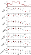 |
Fig. 1. Overview of the properties of our sample as a function of the Hubble stage parameter (HT). From top to bottom: histogram of the number of galaxies in each bin (ΔT = 1); the distribution of the masses of different components, molecular (MH2) and atomic (MHI) gas, the dust (Mdust) and stars (M⋆), respectively; SFR, molecular-to-total gas fraction, and metallicity. Data are represented as gray points, the mean value in each bin of HT is a red circle. In each panel, we indicate the number of galaxies with measurements (and upper limits) for each quantity. This figure is similar to Fig. 1 by C20. |
3. Data analysis
3.1. Methods
In the following sections, scaling relations between two quantities were modeled using the Python package inmix4 (Kelly 2007), a linear regression method based on a Bayesian approach. linmix allowed us to consider errors on both dependent and independent variables and upper limits on the latter. Furthermore, the code includes a free parameter to account for the intrinsic dispersion about the regression (δintr, i.e., not related to measurement uncertainties), which has zero means and standard deviation δintr.
In the case of scaling relations involving three quantities, we could not rely on linmix. In this case, best-fit parameters were obtained by minimizing a log-likelihood function with the emcee package, a pure-Python implementation of Goodman & Weare's affine invariant Markov chain Monte Carlo (MCMC) ensemble sampler (Foreman-Mackey et al. 2013). Then, we adopted the following model for the scaling relation:
 (1)
(1)
In the log-likelihood function, we also included a free parameter to account for the intrinsic dispersion of the value (δintr, i.e., not related to measurement uncertainties), which was summed in quadrature to the uncertainties on both X and Y quantities considered in each relation.
In addition, we used a set of correlation coefficients (CCs, namely Pearson's CC, and Kendall rank CC) to statistically compare different scaling relations. Pearson's CC (P, hereafter) measures the linear correlation between two sets of data. It is the ratio between the covariance of two variables and the product of their standard deviations. Kendall's rank CC (K, hereafter) is a non-parametric hypothesis test that measures the rank correlation between two variables, i.e., if the two datasets show similar orderings when ranked by each of the quantities. It is less affected by outliers with respect to other rank coefficients, such as the Spearman rank CC. These two CCs have values ranging between −1 and 1. Upper limits were excluded in the fitting procedure of scaling relations involving three quantities (Eq. (1)) or the calculation of CCs.
3.2. Radial profiles of CO line brightness
To accurately study the scaling relations between molecular gas and other galaxy properties, it is necessary to map the gas across the entire galactic disk. Observational evidence suggests that molecular gas is mainly concentrated in the central regions of galaxies, with an exponentially radial decreasing distribution with a scale radius that is a fraction of the optical scale radius (e.g., Lisenfeld et al. 2011; Boselli et al. 2014; Casasola et al. 2017). In Fig. 2, we show the radial intensity profile of 67 out of the 121 galaxies presented here. The selected galaxies have publicly available CO intensity maps (see references in the online material). Radial averaged intensities of CO lines are normalized to the intensity at the center of each galaxy (i.e., corresponding to the optical position, retrieved from the DustPedia archive). Radial profiles were extracted with elliptical apertures projected on the plane of the sky based on the galaxy's inclination and position angle. In Fig. 2, galaxies are color-coded based on their morphological type, and divided into four bins based on their Hubble stage number (see the legend in Fig. 2 for further details).
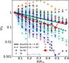 |
Fig. 2. CO emission radial profile, as a function of the optical radius (R25). The CO scale radius (R25) is reported as a vertical gray line. Objects are color coded on the basis of morphological classification. The median radial profile at each radius is represented with red squares. The radial profile predicted by the exponentially decreasing disk by Boselli et al. (2014) is shown as solid and dashed lines, when inclination angles of 30° and 60° are assumed, respectively. |
Fig. 2 shows that individual radial profiles have a significant scatter with respect to the mean radial profile. Nevertheless, the mean is consistent with the model of an exponentially decreasing gas distribution, within the typical uncertainty (i.e., ∼15−20%, including calibration error; e.g., Leroy et al. 2021). This suggests that the adoption of an average exponential profile (Lisenfeld et al. 2011; Boselli et al. 2014; C20) remains a good compromise for estimating total mean gas mass for a sample of galaxies for which only partial observations of the galactic disk are available. However, the large scatter observed in the profiles implies that each galaxy has some deviations from the mean profile, which does not assure a correct estimate of the total  for individual galaxies, and hence of MH2, when the average trend is used (see Appendix B for more details). For this reason, in this work, we have collected and used data from the most recent surveys that have mapped the molecular gas over a significant portion of the galaxy's optical disk (>70%; see Section 2.2).
4. Scaling relations
Here, we investigated scaling relations between different ISM components and other galaxy properties (namely, SFR, M⋆, Mdust) in a homogeneous sample of late-type (HT>0) galaxies. In particular, we focused on the analysis of the molecular gas component, the fuel of star formation, to identify possible physical conditions and host-galaxy properties that enhance molecular hydrogen in galaxies. To this goal, we characterized a collection of correlations in terms of slope, normalization, and intrinsic dispersion (δintr; i.e., the dispersion that is not owed to measurement uncertainties), as described in Section 3. In the end, we compared and ranked scaling relations between MH2 and other galaxy properties (or a combination of properties) to determine the relation that has a lower intrinsic scatter.
4.1. Relations between dust and gas
In Fig. 3, we present the scaling relations between the mass of different gas components, namely the atomic gas within the optical radius (MHI, R25; upper left panel), the total atomic gas (MHI, tot; upper central panel), the molecular gas (MH2; bottom left panel), the total gas mass within the optical radius (Mgas, R25=MH2+MHI, R25; bottom central panel) and measured over the entire disk (Mgas, tot=MH2+MHI, tot; bottom right panel) and the dust mass. In the upper right corner, we also present the relation between M⋆ and Mdust, as stars are one of the key channels to the formation of dust particles (Draine 2003). For a fair comparison, in the six panels of Fig. 3 we display only 120 out of 121 galaxies of the sample described in Section 2.1, as we excluded NGC 1336, which lacks HI measurement (see Section 2.1). We recall that the hydrogen masses presented here have not been corrected for the contribution of heavy elements, from helium onward. Correcting gas masses for heavy elements would require multiplying masses by a constant factor of 1.36 (e.g., C20). This does not affect the determination of the slope or scatter of the relations analyzed in this work; it merely produces a constant offset in their normalization, which can therefore be accounted for straightforwardly. Overall, Mdust shows a strong correlation (P>0.7 and K>0.5) with all the gas components and M⋆ presented in Fig. 3. Focusing on the atomic gas displayed in the upper row of Fig. 3, we observed that the relation MHI, R25 versus Mdust, and MHI, tot vs. Mdust are characterized by sublinear slopes and a relatively large dispersion. Furthermore, the correlation is stronger (i.e., lower intrinsic dispersion and higher CCs) when considereing only the dust and the co-spatial gas, i.e., measured within the optical extent of the galaxy R25, and not the total atomic gas (δintr = 0.37 and 0.43, respectively). This may result from the concentration of most of the dust particles within R25, while the cold atomic gas can extend far beyond these areas.
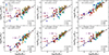 |
Fig. 3. Gas and stellar masses vs. dust mass. In the upper row, the atomic gas mass within R25 (left panel), the total atomic gas mass (central panel), and the stellar mass (right panel) are plotted against the dust mass. In the bottom row, the molecular gas mass (left panel), the total gas mass (atomic plus molecular) measured within the optical radius (central panel), and the total gas mass measured over the entire galactic disk (right panel) are plotted against the dust mass. Data are color coded according to the morphological type (HT). The best-fit parameters for each scaling relation are reported in the upper left corner, while the best-fit line is represented with the solid black line. The 68% confidence interval of the best-fit parameters is represented as a gray-shaded region. The intrinsic dispersion (δ) is reported in the bottom right corner, followed by the correlation coefficients (namely, P and K). |
Regarding the molecular gas component, using MH2 estimates based on maps allowed us to detect a tight correlation between dust and molecular gas. This correlation is stronger than the one inferred using MH2 values extrapolated from pointed observations, and it is also stronger than that between dust and the atomic component (see Appendix A for a detailed comparison with C20). The MH2 vs. Mdust relation (MGD, hereafter) shows a scatter (δintr = 0.38) comparable to that for atomic gas, but with higher CCs (increased by ∼0.15) and a super-linear slope (α = 1.25±0.05). This suggests that galaxies that are richer in molecular gas are proportionally less rich in dust when compared to galaxies at lower masses. A significant contribution to the measured intrinsic dispersion is likely driven by the galaxies with HT > 7, which show a wide dispersion across the best-fit relation, particularly in the low mass end regime (log(Mdust/M⊙)<6.5). Among them, NGC 7715 stands out in all panels, except for the M⋆ vs. Mdust relation, with a Mdust that was likely underestimated in the SED fitting procedures due to contrasting fluxes in the far-IR (see Nersesian et al. 2019 and the DustPedia archive5).
Our analysis suggests that massive galaxies are more efficient in converting atomic into molecular gas phase than less massive objects, as the molecular-to-atomic gas mass ratio increases with the stellar mass (see the second panel from the left of Fig. 6), while the dust-to-stellar mass ratio does not – which is why the MGD relation has a super-linear slope. The pressure, which is driven by the surface density of stars with an additional contribution by the gas surface density, enhances the gas density, favoring cooling and the formation of molecules (Elmegreen 1993; Krumholz et al. 2009).
The stellar mass, M⋆, shows a very good correlation with Mdust (P = 0.89, K = 0.65), with an intrinsic dispersion which is smaller than the one that is observed for the relation between single gas components and dust (δintr = 0.29). The slope is just slightly sublinear (α = 0.93±0.05), and holds over almost four orders of magnitude across different mass regimes and morphological types. Nevertheless, there is a minor clustering in terms of HT in the more massive end (Mdust>106.5 M⊙) of the relation, with galaxies with lower HT tend to have higher M⋆ for a given Mdust, consistent with previous results from the literature González Delgado et al. (2015). Galaxies with lower HT (e.g., S0, Sa types) have more stars and less dust because they have almost depleted their gas (lower MH2-to-M⋆ ratio), having formed more stars when compared to higher HT. This makes them older, hence dominated by stellar processes, which lead to an unbalanced dust destruction-to-formation rate. The role of gas pressure in building up larger molecular gas reservoirs will be further discussed in Section 4.2.
In the bottom central and right panels of Fig. 3, we show the relation between the dust mass and the total (atomic plus molecular) gas mass measured within R25 or over the entire galactic disk, respectively. The two correlations are slightly sublinear (slopes are 0.93±0.04 and 0.89±0.05, respectively, and they have the lowest intrinsic dispersion among the relations presented in Fig. 3 (δintr = 0.21, and 0.25, respectively). The relation between co-spatial quantities is stronger (P = 0.86, and P = 0.70) and has lower δintr, confirming what has been discussed above for MHI, tot.
The stronger correlation between global Mdust and MH2 has been confirmed by spatially resolved studies both in our Galaxy (e.g., Lee et al. 2012; Bialy et al. 2015) and in nearby objects (e.g., Wong & Blitz 2002; Leroy et al. 2008; Morselli et al. 2020; Casasola et al. 2022), where molecular gas and dust are observed to be co-spatial to star-forming regions, dense environments rich in gas and dust. However, as found by C20, the relation between the total gas mass, Mgas,R25, co-spatial to Mdust has in fact the lowest intrinsic dispersion (δintr = 0.21±0.02) and higher CCs.
No major clustering in terms of HT was observed in the present sample in any of the scaling relations presented in Fig. 3, except for the M⋆ vs. Mdust relation discussed above.
Minor clustering is mostly due to relatively atomic-rich galaxies at later stages (HT>7), which deviate more from the best-fit relation, as visible also in the Mdust versus total gas mass plot (lower right panel of Fig. 3). This segregation is likely driven by the relatively low content of metals usually observed in such types of galaxies (e.g., Gallazzi et al. 2005).
Using the Mdust-MH2 relation, we also checked that the dispersion is not influenced by the adoption of a common CO-to-H2 conversion factor (see Appendix C) or of a common CO(2–1)-to-(1–0) emission line ratio for the 103 galaxies shown in Fig. A.2. To this last goal, we divided the galaxies with CO(2–1) observations from those with CO(1–0) measurements (22 and 81 objects, respectively). The Ps estimated for the MH2-Mdust correlation for the two subsamples of galaxies do not differ significantly (R = 0.83 and 0.85, respectively).
4.2. Molecular gas main sequence and the global Kennicutt-Schmidt relation
Understanding what drives the formation of molecular gas in galaxies, for a given M⋆ or SFR, allows us to predict how galaxies evolve, e.g., whether they will continue to grow in mass by forming new stars or become passive. To this goal, we investigated with our sample the relation between MH2 and M⋆, also known as Molecular Gas Main Sequence (MGMS, hereafter; e.g., Lin et al. 2019), and the MH2-SFR relation, commonly referred to as the global – or galaxy-integrated – Kennicutt-Schmidt law (gKS, hereafter), to honor the pioneering works by Schmidt (1959) and Kennicutt (1989). These two relations are presented in the left and central panels of Fig. 4, respectively. As discussed in Section 4.1, the molecular gas mass is tightly related to the dust content, which makes the dust a key component to predict MH2, thus we added the MGD relation in the right panel of Fig. 4 for comparison. In all panels of Fig. 4, the 121 galaxies of the entire sample are shown color-coded with their specific star formation rate (sSFR = SFR/M⋆). Here, the MGD includes NGC 1336, which is not included in Fig. 3, due to the missing MHI measurement, but the results are fully consistent with those discussed above. The best-fit parameters obtained from the linmix procedures are reported in each panel and in Table D.1. The gKS is characterized by a close to linear slope, α = 1.09±0.08, while MGMS and MGD are consistently slightly super-linear, α = 1.17±0.07 and 1.26±0.06, respectively. The MGMS shows the link between the molecular gas mass and the stellar mass, the latter being the main contributor to the gravitational potential of the disk in the vast majority of the galaxies in our sample, and always dominates in central regions where most of the molecules reside. Indeed, in recent years, MGMS and gKS have been suggested as fundamental relations for the cycle of star formation (e.g., Lin et al. 2019; Baker et al. 2023), with the linear trend of the gKS relation reflecting the small variations of star formation efficiency. Consequently, the well-known Main Sequence (MS) of star-forming galaxies (e.g., Renzini & Peng 2015) that relates M⋆ and SFR is considered a by-product of both MGMS and gKS (see also Section 4.3). The relevance of other physical parameters, such as the stellar mass, in driving the atomic-to-molecular gas conversion can be seen also in the right panel of Fig. 4: the formation of the hydrogen molecules is enhanced as the mass of dust increases, as already shown in Fig. 3. In addition, the gKS relation implies that the increasingly more intense radiation fields produced by the young stars in galaxies with higher SFR may destroy part of the dust particles surrounding the star-forming regions, hence reducing Mdust in the higher mass regime.
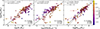 |
Fig. 4. Molecular gas mass scaling relations. From left to right: MH2 vs. M⋆, SFR, and Mdust. Data are color coded for the sSFR. The best-fit parameters for each scaling relation are reported in the upper-left corner, while the best-fit line is represented with a solid black line. The intrinsic dispersion (δ) is reported in the lower-right corner, followed by the correlation coefficients (namely, P and K). |
Comparing MGMS, gKS, and MGD scaling relations, MGD has the lower intrinsic dispersion (δintr = 0.38) and the higher CCs (P = 0.86, K = 0.66) among the relation shown in Fig. 4, suggesting that dust mass can be used as a reliable proxy of the molecular gas reservoir in this sample of galaxies. The MGMS and MGD dispersion shows a weak relation with the sSFR, with galaxies at higher sSFR having possibly a higher molecular gas mass at a given stellar or dust mass (for M*>1010 M⊙ and for Mdust>5×10⁶ M⊙). The deviations at the high mass end of the MGMS relation, visible for galaxies with a low sSFR, reflect the bimodal distribution usually observed in the SFR-M⋆ (MS; e.g., Cano-Díaz et al. 2016; Guo et al. 2015; Renzini & Peng 2015). Galaxies move from the MS to the green valley (e.g., Brownson et al. 2020; Lin et al. 2022), and eventually to the so-called red sequence, i.e., passive objects, as the availability of molecular gas gradually decreases (see the discussion in Section 5.2). This suggests that M⋆ cannot be used alone to accurately predict the amount of molecular gas in a galaxy, and the SFR is required to determine the evolutionary phase of the galaxy accurately.
We note that we did not include MH2 upper limits in the fitting procedures, but they are shown in Fig. 4. MH2 upper limits follow a similar trend to that observed for MH2 detections in the rest of the sample in all scaling relations presented (namely, MGMS, gKS, and MGD), populating the low-M⋆, SFR, and Mdust regimes.
4.3. The fundamental plane for SF
Based on the results from gKS and MGMS, we combined M⋆ and SFR to better constrain MH2. In this case, we fit the relation with Equation (1), as described in Section 3. We also show the projection of the best-fit three-dimensional plane with each of the axes made by M⋆, SFR, and MH2 (x, y, and z-axes, respectively). The best-fit relation is
 (2)
(2)
and intrinsic dispersion  . As mentioned in Section 3, we did not include upper limits on MH2 in this fitting procedure. The intrinsic dispersion estimated in this case is lower than in the case of MGMS, gKS, and MS relations (see Table D.1), suggesting that the connection between the three quantities (namely, MH2, M⋆, and SFR) is tighter than when only two are considered at a time. This way, we removed part of the degeneracy that affects both MGMS and gKS, which comes from the attempt to collapse a multidimensional distribution of galaxy properties onto a linear relation. For illustrative purposes, the collapsed distribution of points on each two-dimensional plane (namely, MH2-M⋆, MH2-SFR, and SFR-M⋆) is shown in the left panel of Fig. 5. To further highlight the relatively low dispersion in the data, we color-coded the points based on their distance from the best-fit plane. From a three-dimensional perspective, combining MH2, M⋆, and SFR, we obtained a more complete view of the current evolutionary stage of galaxies, which are thought to move across this plane. Indeed, several recent studies have suggested the existence of a fundamental plane of SF, such as the one presented in the left panel of Fig. 5 (e.g., Lin et al. 2019; Baker et al. 2023). In this picture, it is clear that only the cycle of star formation relies on the balance between MH2, M⋆, and SFR, as represented by the plane in the parameter space described by the three quantities. As a galaxy grows in mass following the main sequence, it will have an almost linear proportion between its M⋆, MH2, and SFR. If at some point, a galaxy cannot replenish its molecular gas reservoir anymore, which can happen because of several physical mechanisms such as sudden feedback-driven gas removal or heating in its interstellar and cirgumgalactic media (e.g., Peng et al. 2015), these processes will stop its star formation activity within a time which is proportional to the depletion time (tdep∝MH2/SFR). Once the quenched phase begins, the galaxy will deplete its remaining gas reservoir and then it will evolve passively. This will make M⋆ to increase proportionally to the availability of cold gas (but this can also depend on galactic morphology and the gas distribution; e.g., Peng et al. 2010; Saintonge et al. 2016), but at a lower sSFR (i.e., moving to the region of quenched/passive galaxies in Fig. 4). Then, the galaxy will evolve passively, following stellar processes, with a low sSFR level.
 |
Fig. 5. Fundamental plane of SF and ISM. Left panel: MH2 vs. M⋆, and SFR in a three-dimensional projection. Data are color coded as a function of their distance from the best-fit function. The green, blue, and red-shaded heat maps represent the density profiles of the data on the gKS, MGMS, and MS planes, respectively. Contours are shown to better distinguish the density profile, divided into ten levels. The best-fit relation of each two-dimensional panel is color coded according to the data heat maps, while best-fit parameters are listed in Table D.1. Right panel: MH2 vs. MHI, R25, and Mdust in a three-dimensional projection. Color coding is the same as in the left panel. The green, blue, and red-shaded heat maps represent the density profiles of the data on the MH2-MHI, R25, Mdust-MHI, R25, and MGD planes, respectively. |
4.4. The fundamental plane for the ISM
Similarly, we fit Equation (5) to the data, which include Mdust on the x-axes, MHI on the y-axis, and MH2 on the z-axis. In the right panel of Fig. 5, we show the projection of the best-fit three-dimensional plane, with best-fit relation:
 (3)
(3)
and intrinsic dispersion  . First, δintr is larger with respect to that measured in the cases of the MGD and the dust-versus-total gas relation. This suggests that the physical connection between dust and molecular gas is stronger than that between the three main components of the ISM6. Then, the atomic gas trend is almost constant (the corresponding slope is consistent with zero within ∼2−2.5σ) when both dust and molecular gas content increase. This is likely driven by the large scatter that characterizes the distribution of MHI, R25 for a given Mdust and MH2. We found no significant difference considering the total atomic gas mass (MHI, tot) over the atomic gas phase co-spatial to the molecular one (MHI, R25). Given this trend, we concluded that it is not the global cold atomic gas richness in galaxies that drives the molecular gas abundance, but rather the ability of a galaxy to make the gas dense enough to favor the atomic-to-molecular transition (see Section 5.1). In this regard, dust is crucial to prevent the cold molecular gas from dissociating, shielding the gas from ionizing radiation Draine (2003). The best-fit slope associated with Mdust in Equation (3) is super linear, while in MGD it was sublinear, suggesting that the dust content dominates over MHI, R25 to determine the mass of the molecular gas reservoir and can be used to trace MH2. To conclude, it is worth noticing that the accurate determination of Mdust strongly depends on the modeling of the far-IR emission and is limited to galaxies, mostly in the nearby Universe, with their rest-frame far-IR regime (i.e., ∼40−1000 μm) properly sampled (e.g., Clark et al. 2018; Galliano et al. 2018). For this reason, the application of MGD to predict MH2 to large samples of galaxies is limited by the availability of dust masses. However, this problem may be (at least partially) bypassed by using photometric observations that trace the bulk of the dust emission, as shown in the next section.
5. Discussion
5.1. Gas phase transitions
As discussed in Section 4.1, the atomic and molecular phases of gas are closely linked to dust in our sample. Here, we discuss which are the physical conditions that favor molecular gas enrichment. To this goal, in the left panel of Fig. 6 we present the MH2 vs. the co-spatial MHI relation, color-coded as a function of the Hubble type. The plot includes all 120 galaxies presented in Fig. 3. CCs are P = 0.63 and K = 0.47, respectively, which tells us that there is a moderate-to-strong correlation between the two co-spatial gas phases, yet there is also a significant scatter. Later-type galaxies are those that are deviating most from the main trend, with a larger atomic-to-molecular gas ratio. However, their relatively low statistics did not impact the global trend of the sample and the CCs (P and K are 0.68 and 0.4,8, limiting the sample to HT ≤ 7). This indicates that the dispersion is likely driven by individual galaxy characteristics, such as differences in morphology, stellar mass, or accretion history. When dividing our sample between galaxies in clusters (e.g., the Virgo Cluster; Corbelli et al. 2012; Brown et al. 2021) and field galaxies, the environment does not seem to impact this relation, as cluster and field objects show similar trends.
 |
Fig. 6. Left panel: Molecular gas mass vs. atomic gas mass. Data are color coded according to the morphological type as in Fig. 3. The best-fit line is represented with a solid black line, and the gray-shaded region represents the 68% confidence interval of the posterior distribution of the parameters. The intrinsic dispersion (δintr) and correlation coefficients (namely, P and K) are reported in the lower part of each panel. Central left panel: Molecular gas fraction vs. stellar mass. Central right panel: Molecular gas fraction vs. dust-to-stellar mass ratio. Right panel: Molecular-to-total gas fraction vs. DTGR. The black cross represents the median error on both the x and y-axis. |
In the central left panel of Fig. 6, we show the molecular-to-atomic gas mass ratio (H2-to-HI) as a function of the stellar mass. The P index suggests a moderate correlation ( = 0.5), but the scatter is quite large (δintr = 0.56), as highlighted by the value of K ( = 0.25). However, as discussed for the MGMS, we suggest that the positive trend of this correlation is a direct consequence of the gravitational potential driven by the stars (see discussion in Section 4.2) that favors the formation of the cold gas reservoir.
In the central right panel of Fig. 6, the segregation of galaxies according to their HT is likely driven by M⋆, which increases when HT decreases (see Fig. 1 for a binned view of this trend). The H2-to-HI ratio increases from galaxies with higher HT (and lower M⋆) to earlier-type (and more massive) ones. In the right panel of Fig. 6, we plot the molecular gas fraction as a function of the dust-to-total-gas ratio (DTGR). Galaxies with HT>7 show a low molecular fraction for a variety of DTGR ratios, while galaxies with HT≤7 are distributed across the whole range of molecular fractions and have 0.0016≲DGR≲0.016, although the distribution peaks at DTGR ≃0.004. The galaxy's ability to increase its dust mass depends on the balance between stellar processes that create new dust grains and those that destroy them. The sublinear slope of the MGD suggests that, at higher masses, dust might be destroyed more efficiently than at lower masses, and this also explains the marginal dependence of the molecular fraction on the DTGR and the marginal dependence of the DTGR on the galaxy Hubble-type.
Indeed, despite the strong correlation and relatively low intrinsic dispersion found for the MGD relation in Section 4.2, Fig. 6 highlights the crucial role of M⋆through the local gravity in driving the formation of molecules. The anticorrelation we found between the molecular gas fraction and the dust-to-stellar mass ratio for our sample confirms that the process of atomic-to-molecular gas conversion is more efficient for high stellar masses rather than for high dust masses as soon as atomic gas is available.
5.2. Molecular gas fraction and star formation efficiency
As discussed above, classical scaling relations between MH2, M⋆, and SFR suffer from the contamination of galaxies facing different evolutionary phases. Specifically, in Section 4.2, we discuss the presence of passive galaxies in the MGMS as those galaxies having a relatively low sSFR due to a relatively low molecular gas-to-star ratio (MH2/M⋆). To this goal, we plot the MH2/M⋆ as a function of the sSFR in the left panel of Fig. 7. The ratio between MH2 and M⋆ indicates the amount of molecular gas that is available to sustain the growth of the galaxy, given the mass of stars already formed. The sSFR is an important parameter to describe how fast a galaxy has grown since 1/sSFR indicates the timescale that the galaxy would have needed to build the current mass at the current SFR. Therefore, the diagram shown in the left panel of Fig. 7, allows us to distinguish quiescent (or soon-to-be quiescent) galaxies from those that are in a relatively active build-up phase. Indeed, earlier-type galaxies from our sample (HT ≤ 3) show relatively low molecular gas fraction and low sSFR (<10−10 yr−1). Conversely, later type galaxies, HT >7, are mostly molecular gas-poor, but they are growing at a sustained rate (sSFR>10−10 yr−1). This subsample may also include galaxies that are classified as irregular, which can be a consequence of a tidal interaction with a close companion galaxy. Even if mergers are not frequent in the local Universe (∼2%; Casteels et al. 2014), past interactions with nearby galaxies can induce instabilities in the disks of galaxies, which can enhance the star formation even in relatively gas-poor objects. In between these two classes, there is the bulk of our sample (71 out of 121 galaxies) that has a median MH2-to-M⋆ ratio of about 0.1.
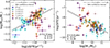 |
Fig. 7. Left panel: Molecular-to-stellar mass ratio vs. sSFR. Data are color coded according to the morphological type, as in Fig. 3. The best-fit line is represented with a solid black line, and the gray-shaded region represents the 68% confidence interval of the posterior distribution of the parameters. The intrinsic dispersion (δintr) and correlation coefficients (namely, P and K) are reported in the lower (upper) right corner of the left (right) panel. Right panel: Star formation efficiency vs. stellar mass. |
The distinction between two types of molecular gas-poor galaxies is evident in the right panel of Fig. 7, where later type galaxies are relatively efficient at forming stars, with a mean star formation efficiencies (SFE=SFR/MH2<10−8 yr−1) higher than the bulk of the sample, although with a large scatter, while early types with HT <7 have SFE similar to later type galaxies with similar stellar mass (the median value being ∼10−9 yr−1) irrespective of their MH2-to-M⋆ ratio). From an evolutionary perspective, the HT > 7 galaxies in our sample represent those galaxies still in a growth phase, with the highest SFE. Their future evolution depends on their ability to convert their atomic gas reservoir into molecular gas, sustaining their star formation. These galaxies exhibit some of the highest atomic-to-molecular gas ratios in our sample (see Fig. 6 and the discussion below). Conversely, the relatively low SFE of galaxies with HT ≤ 7 suggests they could have entered a quenching phase. We underline that there is no evidence of chemical evolution between 3 < HT ≤ 7 and HT ≤ 3 objects since they show similar metallicity and similar DTGR, as shown in Fig. 6. To conclude, in this analysis, we underline that we did not find differences between field and cluster galaxies (e.g., from the Virgo cluster; Corbelli et al. 2012; Brown et al. 2021), since both classes of sources share similar properties (e.g., sSFR, SFE) when paired for morphological types.
6. An alternative approach to trace gas reservoirs
6.1. Molecular gas
To avoid limitations of using physical quantities derived from galaxy models, such as Mdust, M⋆, and SFR, we tested the reliability of photometric measurements as a proxy of MH2and MHI, R25. We collected photometric data from the UV to far-IR wavelengths from the DustPedia database (see Clark et al. 2018 for details), considering all the photometric bands from Clark et al. (2018), except for Spitzer IRAC 1 and 2 bands (because these cover similar wavelength ranges of WISE band 1 and 2, and all objects targeted by the IRAC instrument already had WISE observations). Similarly, we did not consider Spitzer MIPS 70 and 160 bands, since Herschel PACS 70 and 160 cover the same wavelength regimes. We complemented the limited number of photometric observations from PACS 70 (available for 64 out of 121 galaxies), using Spitzer MIPS 70 data for 21 galaxies that lack Herschel PACS 70 data. This way, we had 85 galaxies with a monochromatic luminosity at 70 μm.
In Appendix F in Fig. E.1, we showed the relations between  (i.e., MH2 divided by the constant αCO = 3.26 M⊙ pc−2 (K km s−1)−1, and converted into units of solar luminosity, L⊙) and the luminosity measured within each photometric filter. Since the photometric coverage is not uniform for the entire sample of 121 objects, we tested the correlation between
  and the luminosity in each band for two different sample selections: i) by crossmatching all photometric measurements, we selected a subsample of 47 objects that have a measurement in all the bands (sample A); ii) we considered all galaxies having a photometric measurement in each band (sample B). This allowed us to compare the results of the correlation between
  and the luminosity of the galaxy at different wavelengths on a common sample (sample A), but also to explore each correlation using better statistics (sample B). Both best-fit lines are represented in Fig. E.1 and the subsamples are color-coded accordingly. In Table D.1, we provided the best-fit parameters and CCs for each correlation between
  and νLν.
The best-fit relations obtained for samples A and B are in general agreement in each band, with deviations that become significant only in GALEX bands, given the significantly higher number of galaxies in sample B than in sample A. The intrinsic dispersion measured for sample A is almost systematically smaller than that measured for sample B, likely due to a combination of lower statistics and a greater homogeneity in the former sample. Based on the CCs shown in each panel of Fig. E.1 and δintr reported in Table D.1,  better correlates with the luminosities measured in mid-IR and far-IR bands, with P and K larger than 0.7. In particular, the tight relation between
  and the luminosity in WISE band 3 and Spitzer IRAC 8.0 μm in the mid-IR is likely driven by the presence of polycyclic aromatic hydrocarbons (PAH) features that dominate the emission in those bands (e.g., Whitcomb et al. 2023). Indeed, PAH are emission features that are tightly related to star formation activity (e.g., Cortzen et al. 2019; Zanchettin et al. 2024), and they are usually observed in actively star-forming galaxies. However, given that similar but steeper correlations hold also in early-type galaxies (Gao et al. 2025) because old stars also contribute to the mid-IR emission, and because of the inference of AGN activity on PAH emission (e.g., García-Bernete et al. 2022; Salvestrini et al. 2022), future studies are needed to better understand the use of 12 μm emission as a proxy for
  . All mid-IR bands have lower values of CCs than FIR bands because hot dust does not represent the bulk of dust mass available in the dense ISM.
The tight correlation between far-IR bands and  reflects that observed between MH2 and Mdust, already discussed in Sections 4.1 and 4.2. All luminosities measured in the 100−500 μm range are good proxies for the molecular gas luminosity, with P≥0.85, with Herschel SPIRE 250 having the highest CCs among all bands (e.g., P∼0.92; see Fig. E.1 and Table D.1 in Appendix D for CCs and best-fit parameters).
Concerning the correlations between UV bands (namely, GALEX FUV and NUV filters) and  , we found a large dispersion and low CCs. UV bands are commonly used to derive the SFR estimates, which roughly cover the star formation activity that occurred over the last ∼100–300 Myr (Kennicutt & Evans 2012, see also the discussion on SFR recipes in Appendix C). However, UV bands only trace the unobscured star formation and need to be corrected for the emission absorbed by dust. This can also significantly affect optical observations at shorter wavelengths, as in the case of the SDSS u filter. Dust obscuration is also dependent on the dust geometry, as well as the inclination of the galaxy with respect to the line of sight.
While stellar mass is a relatively good proxy of the molecular gas mass, individual photometric bands dominated by the stellar emission (namely, SDSS and 2MASS filters) show relatively low CCs (P = 0.66−0.8, K∼0.5) compared to the mid-IR ones, and cannot be considered a good proxy for  in our sample. This limitation might arise because of the small range of luminosities covered by the bulk of our sample, with only a few galaxies extending to low luminosities. For this reason, we suggest using the
  -νLν scaling relations to predict the molecular gas emission with optical to near-IR photometric measurement only for log(νLν/L⊙)>9.5.
To conclude, we suggest that far-IR emission at wavelengths ≥100 μm is the best proxy of  over three orders of magnitude, providing a reliable approach to measure the molecular gas mass when (sub)millimeter observations are not available. In addition, the emission arising due to more prominent PAH features at 7.7 and 11.3 μm is a relatively reliable tracer of MH2, still covering a similar dynamical range in
  .
.
6.2. Atomic and total gas
We also tested if any monochromatic luminosity can be used as a proxy for the atomic gas and total (H2 + HI) gas masses using subsamples A and B. Best-fit parameters are listed in Tables E.2 and E.3, while best-fit lines are shown in Figs. E.2 and E.3. In general, the atomic gas mass, MHI, R25 shows a lower level of correlation (in terms of CCs) and a higher dispersion (i.e., larger δintr) with monochromatic luminosities, when compared to  . At the longest far-IR wavelengths (namely, Herschel SPIRE observations), MHI, R25 shows the tightest relations in terms of intrinsic dispersion (δintr = 0.38 dex for SPIRE 500) and highest CCs (P∼0.8 and K>0.6 for SPIRE 500). This is in general agreement with the result presented in Section 4.1. Moreover, the atomic phase shows better correlation parameters with the emission that arises from the cold diffuse dust (SPIRE 500), and the CCs (intrinsic dispersion) decrease (increase) monotonically going at short wavelengths down to WISE4 and Spitzer 24 bands. This is the first difference between MHI, R25 and
  , with the latter that correlates best with monochromatic emission close to the peak of the far-IR SED. Furthermore, we found that MHI, R25 shows a relatively good correlation with UV/optical luminosities (namely, GALEX FUV, NUV, and SDSS u bands), only slightly less significant than with FIR luminosities, in contrast with the results for
  .
.
As expected, the atomic phase of gas is not directly involved in recent star formation events, and MHI, R25 does not strongly correlate with SFR tracers (e.g., PAH features, warm dust emission; see Kennicutt & Evans 2012). However, the good correlation between MHI, R25 and NUV suggests that the atomic gas reservoir is needed to sustain the galaxy's ability to form new stars, it provides the gas fuel to sustain star formation over a long time interval, 300–500 Myr, for several lifecycles of molecular clouds (15 Myr, Corbelli et al. 2017). Over this period, star formation can be traced by emission in the NUV band.
The HI gas also establishes a good correlation with 500 μm emission, a good proxy of the diffuse dust component. Regarding the total gas mass within R25, we found an overall improvement of CCs when analyzing the correlations with monochromatic luminosities in the optical bands. As for  , the strongest correlations for Mgas,R25 are established with the far-IR bands (P>0.85 and K≳0.7). Slopes are in this case close to linear, slightly flatter than for
  .
.
6.3. Dust content
Similarly to previous sections, we investigated the best proxies of the dust mass among monochromatic luminosities. Looking at Fig. E.4, as expected the best proxies for Mdust are the monochromatic luminosities at wavelengths longer than 160 μm, (from whose fit Mdust is derived) which show strong correlations (P>80 and K≥70) and relatively low dispersion (δintr≤0.1 dex at 500 μm). However, if FIR observations are not available, strong correlations (P>0.8 and K≥0.7) can be found between Mdust and the luminosities from optical to mid-IR wavelengths, up to WISE3 (i.e., ∼8 μm). The tight connection between dust mass and optical or near-IR emission is likely a consequence of the tight correlation between Mdust and M⋆ (e.g., McGaugh & Schombert 2014), already shown in Section 4.1, with a scaling close to linear. The intensity of PAH emission features falling within the WISE1, WISE2, and WISE3 bands suggests the use of luminosities in these bands as a proxy for Mdust. The scaling is, however, non-linear. The reason for this is not yet clear because how PAH molecules form is still a matter of debate, with some dust evolution models that predict PAHs formation by fragmentation of large carbonaceous grains (e.g., Seok et al. 2014), while observations on the Small Magellanic Clouds support models with PAHs that forms in molecular clouds (e.g., Sandstrom et al. 2010).
Our conclusions for the best reliable proxies of the different phases of the ISM are the following: i) emission at far-IR wavelengths (particularly from 250 to 500 μm) can be used as a proxy of all cold gas phases and dust in the ISM. ii) If observations in the FIR are unavailable, the monochromatic luminosity measured in mid-IR bands where PAH features fall is also a very good tracer for the molecular gas and the dust mass (P>0.8, K≥0.7, and δintr<0.3 dex). iii) The dust content is also traced with good approximation (δintr<0.3 dex) by the optical and near-IR luminosities. iv) The NUV luminosity can be used to estimate MHI, R25, but the intrinsic scatter of the relation would allow us to estimate MHI, R25 with a ∼0.4 dex uncertainty.
7. Conclusions
In this work, we selected a large sample of late-type galaxies (121) in the nearby Universe, which have been fully mapped in CO and at FIR luminosities and therefore have reliable estimates of molecular gas and dust masses. Using the DustPedia database, we complemented these data with estimates of other physical properties, such as the SFR, HI, and stellar masses, to investigate the physical processes that drive the star formation cycle as galaxies evolve. The main results can be summarized as follows:
-
The global dust mass correlates better with the molecular rather than with the atomic gas mass, in agreement with resolved observations. The use of measurements of CO emission over a large part of the optical extent (>70% R25) of a galaxy was a key element in reaching this conclusion.
-
We confirmed the important role of stellar populations in driving the formation of molecules because their gravity in the disk enhances the gas density.
-
Determining MH2, M⋆, and SFR is necessary to properly understand the evolutionary stage of a galaxy and the emergence of a quenching phase. We determined the fundamental plane of star formation for late-type galaxies characterized by a lower intrinsic dispersion than MGMS and gKS relations.
-
Mdust is the quantity that best correlates with the gas mass in late-type galaxies (i.e., it has the lowest intrinsic dispersion), whether this is molecular or total gas mass. Dust is cospatial with molecular gas and plays a crucial role in the formation of molecules themselves. However, dust production and destruction processes limit the growth of dust masses, and galaxies in the highest stellar mass regime are more efficient in converting atomic into molecular gas, even with a lower dust content.
-
Monochromatic luminosities measured in the FIR at 250–500 μm are the best proxies of atomic and molecular gas masses. In the absence of FIR data, luminosities in mid-IR photometric bands that collect PAH emission can be used to trace molecular gas and dust masses.
Finally, we would like to underline the importance of the availability of CO maps for a reliable estimate of the global molecular content of late-type galaxies, as shown in Section 3.2 and Appendix B. This is due to the large scatter shown by the radial profile of the CO surface brightness. In fact, although the model of an exponentially decreasing molecular gas mass surface density, often adopted in the literature (e.g., Boselli et al. 2014), is a good proxy for the mean molecular gas radial profile of a galaxy sample, individual galaxies can show strong departures from it. This, in turn, implies large uncertainties in molecular mass estimates if CO maps are not available. With future radio interferometers, we also hope to increase the availability of 21-cm resolved gas maps and improve the estimates of atomic gas in the star-forming regions of late-type galaxies. These maps are also necessary to fully understand the baryonic cycle in resolved regions of galaxies, from the center to the galaxy outskirts, where the ISM is mostly atomic.
Data availability
The main properties of the 121 galaxies presented in this work are collected in a table that is only available at the CDS via anonymous ftp to cdsarc.cds.unistra.fr (130.79.128.5) or via https://cdsarc.cds.unistra.fr/viz-bin/cat/J/A+A/699/A346
Acknowledgments
We acknowledge V. Casasola for helpful discussions that improved the presentation of results and E. Liuzzo for her support in defining the sample. This work benefits from the financial support by the National Operative Program (Programma Operativo Nazionale-PON) of the Italian Ministry of University and Research “Research and Innovation 2014–2020”, Project Proposals CIR01_00010. F. S. acknowledges financial support from the PRIN MUR 2022 2022TKPB2P – BIG-z, Ricerca Fondamentale INAF 2023 Data Analysis grant “ARCHIE ARchive Cosmic HI & ISM Evolution”, Ricerca Fondamentale INAF 2024 under project “ECHOS” MINI-GRANTS RSN1. S. B., E. C. acknowledge funding from the grant PRIN MIUR 2017 – 20173ML3WW_001 and from INAF minigrant 2023 SHAPES. F. S., S. B., E. C. acknowledge funding from the INAF mainstream 2018 program “Gas-DustPedia: A definitive view of the ISM in the Local Universe”. F. S., S. B. acknowledge funding from the INAF minigrant 2022 program “Face-to-face with the Local Universe: ISM's Empowerment (LOCAL)”. This work made use of HERACLES, “The HERA CO-Line Extragalactic Survey” (Leroy et al. 2009). This work made use of THINGS, “The HI Nearby Galaxy Survey” (Walter et al. 2008). This publication made use of data from COMING, CO Multi-line Imaging of Nearby Galaxies, a legacy project of the Nobeyama 45-m radio telescope. Software: ASTROPY (Astropy Collaboration 2013); EMCEE (Foreman-Mackey et al. 2013); LINMIX (Kelly 2007); MATPLOTLIB (Hunter 2007); NUMPY (Harris et al. 2020); SCIPY (Virtanen et al. 2020).
The 7 m antenna array at the Atacama site is also known as the Atacama Compact Array (ACA).
Here, we did not include the ionized gas phase, which has a negligible contribution to the total ISM mass; e.g., Draine (2011).
References
- Accurso, G., Saintonge, A., Catinella, B., et al. 2017, MNRAS, 470, 4750 [NASA ADS] [Google Scholar]
- Amorín, R., Muñoz-Tuñón, C., Aguerri, J. A. L., & Planesas, P. 2016, A&A, 588, A23 [NASA ADS] [CrossRef] [EDP Sciences] [Google Scholar]
- Astropy Collaboration (Robitaille, T. P., et al.) 2013, A&A, 558, A33 [NASA ADS] [CrossRef] [EDP Sciences] [Google Scholar]
- Baker, W. M., Maiolino, R., Belfiore, F., et al. 2023, MNRAS, 518, 4767 [Google Scholar]
- Bialy, S., Sternberg, A., Lee, M. -Y., Le Petit, F., & Roueff, E. 2015, ApJ, 809, 122 [NASA ADS] [CrossRef] [Google Scholar]
- Bianchi, S., Casasola, V., Corbelli, E., et al. 2022, A&A, 664, A187 [NASA ADS] [CrossRef] [EDP Sciences] [Google Scholar]
- Bolatto, A. D., Wolfire, M., & Leroy, A. K. 2013, ARA&A, 51, 207 [CrossRef] [Google Scholar]
- Boquien, M., Burgarella, D., Roehlly, Y., et al. 2019, A&A, 622, A103 [NASA ADS] [CrossRef] [EDP Sciences] [Google Scholar]
- Boselli, A., Cortese, L., Boquien, M., et al. 2014, A&A, 564, A66 [NASA ADS] [CrossRef] [EDP Sciences] [Google Scholar]
- Brown, T., Wilson, C. D., Zabel, N., et al. 2021, ApJS, 257, 21 [NASA ADS] [CrossRef] [Google Scholar]
- Brownson, S., Belfiore, F., Maiolino, R., Lin, L., & Carniani, S. 2020, MNRAS, 498, L66 [NASA ADS] [CrossRef] [Google Scholar]
- Calzetti, D., Wu, S. Y., Hong, S., et al. 2010, ApJ, 714, 1256 [NASA ADS] [CrossRef] [Google Scholar]
- Cano-Díaz, M., Sánchez, S. F., Zibetti, S., et al. 2016, ApJ, 821, L26 [Google Scholar]
- Casasola, V., Hunt, L., Combes, F., & García-Burillo, S. 2015, A&A, 577, A135 [NASA ADS] [CrossRef] [EDP Sciences] [Google Scholar]
- Casasola, V., Cassarà, L. P., Bianchi, S., et al. 2017, A&A, 605, A18 [NASA ADS] [CrossRef] [EDP Sciences] [Google Scholar]
- Casasola, V., Bianchi, S., De Vis, P., et al. 2020, A&A, 633, A100 [NASA ADS] [CrossRef] [EDP Sciences] [Google Scholar]
- Casasola, V., Bianchi, S., Magrini, L., et al. 2022, A&A, 668, A130 [NASA ADS] [CrossRef] [EDP Sciences] [Google Scholar]
- Casteels, K. R. V., Conselice, C. J., Bamford, S. P., et al. 2014, MNRAS, 445, 1157 [NASA ADS] [CrossRef] [Google Scholar]
- Chung, E. J., Yun, M. S., Verheijen, M. A. W., & Chung, A. 2017, ApJ, 843, 50 [Google Scholar]
- Clark, C. J. R., Verstocken, S., Bianchi, S., et al. 2018, A&A, 609, A37 [NASA ADS] [CrossRef] [EDP Sciences] [Google Scholar]
- Corbelli, E., Bianchi, S., Cortese, L., et al. 2012, A&A, 542, A32 [NASA ADS] [CrossRef] [EDP Sciences] [Google Scholar]
- Corbelli, E., Braine, J., Bandiera, R., et al. 2017, A&A, 601, A146 [NASA ADS] [CrossRef] [EDP Sciences] [Google Scholar]
- Cortese, L., Ciesla, L., Boselli, A., et al. 2012, A&A, 540, A52 [NASA ADS] [CrossRef] [EDP Sciences] [Google Scholar]
- Cortzen, I., Garrett, J., Magdis, G., et al. 2019, MNRAS, 482, 1618 [NASA ADS] [CrossRef] [Google Scholar]
- Curran, S. J., Polatidis, A. G., Aalto, S., & Booth, R. S. 2001, A&A, 368, 824 [NASA ADS] [CrossRef] [EDP Sciences] [Google Scholar]
- Dale, D. A., Aniano, G., Engelbracht, C. W., et al. 2012, ApJ, 745, 95 [NASA ADS] [CrossRef] [Google Scholar]
- Davies, J. I., Baes, M., Bianchi, S., et al. 2017, PASP, 129, 044102 [NASA ADS] [CrossRef] [Google Scholar]
- De Vis, P., Jones, A., Viaene, S., et al. 2019, A&A, 623, A5 [NASA ADS] [CrossRef] [EDP Sciences] [Google Scholar]
- den Brok, J. S., Chatzigiannakis, D., Bigiel, F., et al. 2021, MNRAS, 504, 3221 [NASA ADS] [CrossRef] [Google Scholar]
- Draine, B. T. 2003, ARA&A, 41, 241 [NASA ADS] [CrossRef] [Google Scholar]
- Draine, B. T. 2011, Physics of the Interstellar and Intergalactic Medium (Princeton, NJ: Princeton Univ. Press) [Google Scholar]
- Ellison, S. L., Thorp, M. D., Lin, L., et al. 2020, MNRAS, 493, L39 [CrossRef] [Google Scholar]
- Ellison, S. L., Wong, T., Sánchez, S. F., et al. 2021, MNRAS, 505, L46 [NASA ADS] [CrossRef] [Google Scholar]
- Elmegreen, B. G. 1993, ApJ, 411, 170 [NASA ADS] [CrossRef] [Google Scholar]
- Figueira, M., Pollo, A., Małek, K., et al. 2022, A&A, 667, A29 [NASA ADS] [CrossRef] [EDP Sciences] [Google Scholar]
- Foreman-Mackey, D., Hogg, D. W., Lang, D., & Goodman, J. 2013, PASP, 125, 306 [Google Scholar]
- Gallazzi, A., Charlot, S., Brinchmann, J., White, S. D. M., & Tremonti, C. A. 2005, MNRAS, 362, 41 [Google Scholar]
- Galliano, F., Galametz, M., & Jones, A. P. 2018, ARA&A, 56, 673 [Google Scholar]
- Gao, Y., Wang, E., Tan, Q. -H., et al. 2025, ApJ, 979, 105 [Google Scholar]
- García-Bernete, I., Rigopoulou, D., Alonso-Herrero, A., et al. 2022, MNRAS, 509, 4256 [Google Scholar]
- González Delgado, R. M., García-Benito, R., Pérez, E., et al. 2015, A&A, 581, A103 [Google Scholar]
- Groves, B. A., Schinnerer, E., Leroy, A., et al. 2015, ApJ, 799, 96 [Google Scholar]
- Guo, K., Zheng, X. Z., Wang, T., & Fu, H. 2015, ApJ, 808, L49 [NASA ADS] [CrossRef] [Google Scholar]
- Harris, C. R., Millman, K. J., van der Walt, S. J., et al. 2020, Nature, 585, 357 [NASA ADS] [CrossRef] [Google Scholar]
- Hunter, J. D. 2007, Comput. Sci. Eng., 9, 90 [NASA ADS] [CrossRef] [Google Scholar]
- Jones, A. P., Fanciullo, L., Köhler, M., et al. 2013, A&A, 558, A62 [NASA ADS] [CrossRef] [EDP Sciences] [Google Scholar]
- Kelly, B. C. 2007, ApJ, 665, 1489 [Google Scholar]
- Kennicutt, R. C. Jr. 1989, ApJ, 344, 685 [CrossRef] [Google Scholar]
- Kennicutt, R. C., & Evans, N. J. 2012, ARA&A, 50, 531 [NASA ADS] [CrossRef] [Google Scholar]
- Köhler, M., Jones, A., & Ysard, N. 2014, A&A, 565, L9 [NASA ADS] [CrossRef] [EDP Sciences] [Google Scholar]
- Krumholz, M. R., McKee, C. F., & Tumlinson, J. 2009, ApJ, 693, 216 [NASA ADS] [CrossRef] [Google Scholar]
- Kuno, N., Sato, N., Nakanishi, H., et al. 2007, PASJ, 59, 117 [NASA ADS] [Google Scholar]
- Lee, M. -Y., Stanimirović, S., Douglas, K. A., et al. 2012, ApJ, 748, 75 [NASA ADS] [CrossRef] [Google Scholar]
- Leroy, A. K., Walter, F., Brinks, E., et al. 2008, AJ, 136, 2782 [Google Scholar]
- Leroy, A. K., Walter, F., Bigiel, F., et al. 2009, AJ, 137, 4670 [Google Scholar]
- Leroy, A. K., Sandstrom, K. M., Lang, D., et al. 2019, ApJS, 244, 24 [Google Scholar]
- Leroy, A. K., Schinnerer, E., Hughes, A., et al. 2021, ApJS, 257, 43 [NASA ADS] [CrossRef] [Google Scholar]
- Lin, L., Pan, H. -A., Ellison, S. L., et al. 2019, ApJ, 884, L33 [NASA ADS] [CrossRef] [Google Scholar]
- Lin, L., Ellison, S. L., Pan, H. -A., et al. 2022, ApJ, 926, 175 [Google Scholar]
- Lisenfeld, U., Espada, D., Verdes-Montenegro, L., et al. 2011, A&A, 534, A102 [NASA ADS] [CrossRef] [EDP Sciences] [Google Scholar]
- Lisenfeld, U., Xu, C. K., Gao, Y., et al. 2019, A&A, 627, A107 [NASA ADS] [CrossRef] [EDP Sciences] [Google Scholar]
- Makarov, D., Prugniel, P., Terekhova, N., Courtois, H., & Vauglin, I. 2014, A&A, 570, A13 [NASA ADS] [CrossRef] [EDP Sciences] [Google Scholar]
- McGaugh, S. S., & Schombert, J. M. 2014, AJ, 148, 77 [Google Scholar]
- Morokuma-Matsui, K., Bekki, K., Wang, J., et al. 2022, ApJS, 263, 40 [NASA ADS] [CrossRef] [Google Scholar]
- Morselli, L., Rodighiero, G., Enia, A., et al. 2020, MNRAS, 496, 4606 [NASA ADS] [CrossRef] [Google Scholar]
- Nersesian, A., Xilouris, E. M., Bianchi, S., et al. 2019, A&A, 624, A80 [NASA ADS] [CrossRef] [EDP Sciences] [Google Scholar]
- Nishiyama, K., & Nakai, N. 2001, PASJ, 53, 713 [Google Scholar]
- Pappalardo, C., Bianchi, S., Corbelli, E., et al. 2012, A&A, 545, A75 [NASA ADS] [CrossRef] [EDP Sciences] [Google Scholar]
- Peng, Y. -J., Lilly, S. J., Kovač, K., et al. 2010, ApJ, 721, 193 [NASA ADS] [CrossRef] [Google Scholar]
- Peng, Y., Maiolino, R., & Cochrane, R. 2015, Nature, 521, 192 [Google Scholar]
- Pettini, M., & Pagel, B. E. J. 2004, MNRAS, 348, L59 [NASA ADS] [CrossRef] [Google Scholar]
- Renzini, A., & Peng, Y. -J. 2015, ApJ, 801, L29 [NASA ADS] [CrossRef] [Google Scholar]
- Saintonge, A., Kauffmann, G., Kramer, C., et al. 2011a, MNRAS, 415, 32 [NASA ADS] [CrossRef] [Google Scholar]
- Saintonge, A., Kauffmann, G., Wang, J., et al. 2011b, MNRAS, 415, 61 [NASA ADS] [CrossRef] [Google Scholar]
- Saintonge, A., Catinella, B., Cortese, L., et al. 2016, MNRAS, 462, 1749 [Google Scholar]
- Salvestrini, F., Gruppioni, C., Pozzi, F., et al. 2020, A&A, 641, A151 [NASA ADS] [CrossRef] [EDP Sciences] [Google Scholar]
- Salvestrini, F., Gruppioni, C., Hatziminaoglou, E., et al. 2022, A&A, 663, A28 [NASA ADS] [CrossRef] [EDP Sciences] [Google Scholar]
- Sandstrom, K. M., Bolatto, A. D., Draine, B. T., Bot, C., & Stanimirović, S. 2010, ApJ, 715, 701 [NASA ADS] [CrossRef] [Google Scholar]
- Schmidt, M. 1959, ApJ, 129, 243 [NASA ADS] [CrossRef] [Google Scholar]
- Seok, J. Y., Hirashita, H., & Asano, R. S. 2014, MNRAS, 439, 2186 [NASA ADS] [CrossRef] [Google Scholar]
- Solomon, P. M., & Vanden Bout, P. A. 2005, ARA&A, 43, 677 [NASA ADS] [CrossRef] [Google Scholar]
- Sorai, K., Kuno, N., Muraoka, K., et al. 2019, PASJ, 71, s14 [Google Scholar]
- Virtanen, P., Gommers, R., Oliphant, T. E., et al. 2020, Nat. Methods, 17, 261 [Google Scholar]
- Walter, F., Brinks, E., de Blok, W. J. G., et al. 2008, AJ, 136, 2563 [Google Scholar]
- Wang, J., Catinella, B., Saintonge, A., et al. 2020, ApJ, 890, 63 [NASA ADS] [CrossRef] [Google Scholar]
- Whitcomb, C. M., Sandstrom, K., Leroy, A., & Smith, J. D. T. 2023, ApJ, 948, 88 [CrossRef] [Google Scholar]
- Wong, T., & Blitz, L. 2002, ApJ, 569, 157 [CrossRef] [Google Scholar]
- Zabel, N., Davis, T. A., Smith, M. W. L., et al. 2019, MNRAS, 483, 2251 [Google Scholar]
- Zanchettin, M. V., Massardi, M., Salvestrini, F., et al. 2024, ApJ, 970, 75 [NASA ADS] [CrossRef] [Google Scholar]
Appendix A: Comparison with MH2 from C20
C20 presented MH2 estimates for 255 late-type DustPedia galaxies. Due to the unavailability of maps for most galaxies, the total  (and thus the total MH2) is estimated from single-pointing observation at the galactic center, assuming an exponential model for the disk. The empirical model is that of Boselli et al. (2014), which is a 3D extension of the model by Lisenfeld et al. (2011); it assumes that the molecular gas density follows an exponential distribution, both along the radius (with scale-radius RCO) and above the plane (with scale-height zCO), and that both scale-lengths are directly proportional to the optical scale-radius (RD25). In particular, C20 assumed RCO/RD25 = 0.17, as found by Casasola et al. (2017) on the largest DustPedia galaxies, and zCO/RD25 = 0.01 as derived by Boselli et al. (2014) from observations and models of edge-on galaxies.
There are 103 galaxies in common between C20 and this work (among which 8 have only upper limits of MH2 from the former and one from the latter). The comparison between MH2 estimates for the galaxies in common is shown in Fig. A.1. There is an overall agreement between the two sets of estimates, but a significant scatter (∼0.35±0.04 dex) is visible. We investigated the objects showing a large variation in the estimate of MH2 from C20 to this work for any selection effect. In particular, we focused on the presence of AGN activity, and any trend with the Hubble stage. Regarding the former, AGN are usually associated with an increased molecular gas emission in the central region (e.g., Solomon & Vanden Bout 2005; Ellison et al. 2021), which may lead to an overestimation of the total MH2 assuming the model by Boselli et al. (2014). Using the classification of active galaxies provided in C20, we did not find any relation between nuclear activity and the object deviating more in MH2 estimate. Indeed, previous studies on local AGN did not find any conclusive results on the systematic difference in terms of MH2 content between AGN and non-AGN galaxies at galactic scales, even if increased global SFR (e.g., Salvestrini et al. 2020, 2022) and SFR surface densities have been observed in the local Universe (e.g., Casasola et al. 2015). Regarding the latter, even if all Hubble stages are not evenly represented in our sample, we did not observe any correlation between the Hubble stage and the offset in MH2. We found it more likely that deviation from the average exponential model is due to the presence of unresolved structures (at the scales of the mm observations available) like bars, which may lead to an increased concentration of molecular gas in the central part of the galaxy.
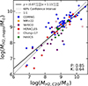 |
Fig. A.1. Comparison of the best-estimates of MH2 presented in this work (y-axes) and retrieved by C20 (x-axes). Objects are color-coded based on the survey from which data were taken. Correlation coefficients (namely, P and K) are reported in the bottom right corner. |
The differences shown in Fig. A.1 are likely driven by the model assumption in extrapolating the global MH2: although the exponential decreasing disk model reproduces well the average radial distribution of the molecular gas, as validated by several literature works (e.g., Lisenfeld et al. 2011; Casasola et al. 2017), it remains an approximation that may tamper the global MH2 determination of single galaxies. This issue is discussed in section 3.2.
In Fig. A.2 we showed the impact of using the new map-derived MH2 estimates on the analysis of scaling relations. The top row (analogous to Fig. 3 in C20) presents the dust mass as a function of the molecular gas mass, for the C20 MH2estimates (left) and for the estimates of this work (right). We remind the reader that the dust mass Mdust is retrieved from the same DustPedia archive both in this work and C20. In the figure, we also indicated the quality of the correlation by using the P (this was used by C20) and the non-parametric CC of Kendall. A major improvement provided by the adoption of MH2 obtained from global mapping of the CO emission results is a tighter relation, with a significant increase in all CCs. When using MH2 detections from C20 (left panel), the correlation has, e.g., a P = 0.74 (0.72 for the full sample of 252 galaxies analyzed by C20). Instead, it is R = 0.86 when using the MH2 detections from the mapping observations we collected in this work. It becomes P = 0.84 when using the 115 galaxies with CO detection. P increases when moving from the Mdust-MH2 relation shown in the left panel to that in the right panel. This indicates that the scaling relation that uses the MH2 of this work shows a lower dispersion, due to a stronger monotonic trend.
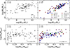 |
Fig. A.2. Effect of the adoption of MH2 from C20 or from this work. Top row: Dust vs molecular gas mass, adopting the MH2 estimate from C20 and presented here (left and right panel, respectively). The correlation coefficients (namely, P and K) are reported in the bottom left corner of both panels. In the right panel, objects are color-coded based on the survey from which the data were taken. MH2 upper limits are marked as shown in the legends. Bottom row: DTGR vs molecular fraction, with MH2 as in the top row. Upper limits and galaxies are shown as described in the corresponding upper panels. |
The use of full map-based MH2 estimates might also prevents the insurgence of spurious trends. An example is shown in the bottom row of Fig. A.2 (analogous to Fig. 14 in C20), where the dust-to-total gas (DTGR) is plotted versus the molecular gas fraction (the C20 MHI,R25 values are used for atomic gas). On their full sample, C20 found a puzzling trend of DTGR increasing with the molecular gas fraction, reaching a maximum, and then decreasing for larger values of the fraction (several possible explanation for the trend are proposed in their section 5.5). The same “hill-like” shape can be seen for the subset of C20 estimates are considered here (left panel). The trend, however, is not present when we used the MH2 presented in this work (right panel): the DTGR shows a shallow increase (P = 0.61 and K = 0.43, respectively) at large molecular-to-total gas ratios (>0.1). The “hill-like” shape found by C20 is likely a consequence of the fact that some of the MH2 provided by C20 for H2-dominated galaxies are overestimated, thus making the DTGR smaller at increasing dominance of the molecular phase over the atomic one.
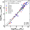 |
Fig. A.3. Comparison of MH2 derived with a constant Milky-Way-like αCO (y-axes) and derived with a αCO based on the prescription by Amorín et al. (2016) (x-axes). Correlation coefficients (namely, P and K) are reported in the bottom right corner. |
Appendix B: Molecular gas masses and metallicity
The CO-to-H2 conversion factor, αCO, strongly depends on the physical conditions (e.g., the presence of highly ionizing radiation fields) and composition (e.g., gas-phase metallicity) of the ISM (see Bolatto et al. 2013 for a detailed review). In section 4, we present the results of our analysis, which are based on the assumption of a constant αCO = 3.26 M⊙ pc−2 (K km s−1)−1 to derive MH2. However, several literature works suggested a strong dependence of the αCO on the gas-phase metallicity (e.g., Bolatto et al. 2013; Accurso et al. 2017). In the right panel of Fig. A.3, we compared the MH2 presented in Sect. 2.2 with those derived with an αCO dependent on the gas-phase metallicity. Among the different recipes for the gas-phase metallicity for DustPedia galaxies provided by De Vis et al. (2019), we opted for that by Pettini & Pagel (2004), which was available for 95 (83) out of 121 (108) galaxies in the present sample (in the sample with Hubble type ≤7;  upper limits are not included). We then adopted the prescription by Amorín et al. (2016), as in C20. In Fig. A.3, the distribution of MH2 obtained with a metallicity-dependent αCO(y-axes) is almost systematically larger (∼1.5−3×) than those obtained with a constant αCO. We tested the impact of the metallicity-dependent αCO assumption on the scaling relations presented in section 4, but we did not find any significant deviation from the trend obtained with a constant αCO, apart from a relatively lower δintr, of the order of a few 0.01 dex. This lower intrinsic dispersion is likely driven by the reduction of the sample size (∼86% of the present one) rather than more accurate MH2 measurements.
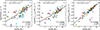 |
Fig. B.1. SFR vs molecular gas mass. Different SFR estimates vs MH2: SFR derived from the SED fitting with CIGALE (Nersesian et al. 2019; left panel), and from the hybrid FUV+24μm recipe (Leroy et al. 2019; right panel]). The 85 galaxies are color-coded by their morphological type. The best-fit parameters for each scaling relation are reported in the upper-left corner, while the best-fit line is represented with the black solid line. The intrinsic dispersion (δintr) is reported in the bottom-right corner, followed by the correlation coefficients (namely, P and K). |
Appendix C: The gKS dependence on the SFR recipe
In section 4.2, we presented the gKs relation for the entire sample of galaxies. The relatively tight correlation represents the physical process (i.e., the star formation activity) that turns the molecular gas into new stars. However, different approaches allow us to estimate the SFR based on different tracers and calibrated in diverse environments (both Galactic and extragalactic; e.g., see Kennicutt & Evans 2012; Figueira et al. 2022). Here, based on the wealth of multiwavelength data of the DustPedia archive, we tested the consistency of the SFR estimates by Nersesian et al. (2019) from the global SED fitting as a good proxy of the ongoing star formation activity to study the gKS. To this end, we considered two independent SFR estimates by using the prescriptions by Kennicutt & Evans (2012): i) the far-UV luminosity corrected for obscuration by using the mid-IR luminosity at 24μm; the 160μm luminosity as a proxy of the peak of the dust reprocessed emission in the far-IR. All three prescriptions allowed us to determine the SFR averaged over a timescale of ∼100 Myr. We referred to Kennicutt & Evans (2012) for a detailed discussion on the timescales probed by different SFR diagnostics. For homogeneity reasons, the analysis was limited to 85 sources out of the 121 objects from the sample presented in section 4.2, since we required each galaxy to be observed in all three bands (namely, far-UV, at 24μm, and at 160μm). No upper limits on MH2 were present in this subsample. In Fig. B.1, we presented the correlation between MH2 (y-axes) and the SFR estimates (x-axes) derived from the SED fitting (SFRSED, left panel), with hybrid UV+IR proxy (SFRFUV+24μm, central panel), and from the far-IR luminosity at 160μm (SFR160μm, right panel). The slopes of the relations shown in the first two panels from the left of Fig. B.1 are fully consistent within uncertainties (0.58±0.06 and 0.56±0.06, respectively), while the SFRFUV+24μm-MH2 relation has a steeper slope (0.76±0.04; see Appendix D and Table D.1 for best-fit parameters). Furthermore, the relation between SFR160μm and MH2 is the strongest in terms of CCs, and with the lowest intrinsic scatter (δintr = 0.24) among the three relations presented in Fig. B.1. While the SFRs estimated from the SED fitting and with the hybrid UV-IR proxy show relatively strong CCs with the molecular gas mass (e.g., P = 0.73 and 0.78, and K = 0.61 and 0.64, respectively), the MH2-SFR160μm is characterized by a strong correlation (e.g., P = 0.89, K = 0.7, respectively). This tight trend results from the physical connection between the molecular gas reservoir and the dust heated by the emission from young massive stars around star-forming regions (e.g., Calzetti et al. 2010, and reference therein). Alternatively, the emission at 160 μm is proportional to the dust content, since the emission close to the peak of the far-IR bump is associated with the dust heated by the interstellar radiation field (e.g., Bianchi et al. 2022). The tight correlation shown in the right panel of Fig. B.1 can represent the connection between MH2 and Mdust. This suggests caution in using SFR160μm as a proxy for SFR. On the other hand, the SFRFUV+24μm leads to results generally consistent with those from the global SED fit of a galaxy. We further discussed the relation between the far-IR emission and the molecular gas content in section 6. Regarding the SFR estimate derived from the SED fitting, the dispersion of the relation with MH2 is likely driven in the first case by potential degeneracy between different models (e.g., dusty star formation and older stellar population), which can be difficult to disentangle, especially in the case of low luminosity regimes. Indeed, this is likely the case of the sources with HT>7 that lie in the central lower region of the left panel of Fig. B.1, which likely have their SFR overestimates from the SED fitting, compared to that derived from the 160μm emission. Given their morphological classification, we expected them to have relatively low SFR and a larger population of old stars. The same issue is likely affecting the correlation in the central panel of Fig. B.1, where the UV-corrected emission is likely overestimated. Here, we showed that the dispersion of the gKS can be reduced by adopting an accurate prescription for the SFR, which can be particularly important in the case of galaxies spanning a wide range of morphological types.
Appendix D: Results of the analysis of scaling relations
2D Scaling relations
3D Scaling relations
Appendix E: Figures and tables of section 6
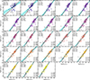 |
Fig. E.1.
|

 vs. monochromatic luminosities
MHI,R25 vs. monochromatic luminosities
Mgas,R25 vs. monochromatic luminosities
Mdust vs. monochromatic luminosities
All Tables
Summary of properties and statistics of the data collected from literature works.
All Figures
|
Fig. 1. Overview of the properties of our sample as a function of the Hubble stage parameter (HT). From top to bottom: histogram of the number of galaxies in each bin (ΔT = 1); the distribution of the masses of different components, molecular (MH2) and atomic (MHI) gas, the dust (Mdust) and stars (M⋆), respectively; SFR, molecular-to-total gas fraction, and metallicity. Data are represented as gray points, the mean value in each bin of HT is a red circle. In each panel, we indicate the number of galaxies with measurements (and upper limits) for each quantity. This figure is similar to Fig. 1 by C20. |
| In the text | |
|
Fig. 2. CO emission radial profile, as a function of the optical radius (R25). The CO scale radius (R25) is reported as a vertical gray line. Objects are color coded on the basis of morphological classification. The median radial profile at each radius is represented with red squares. The radial profile predicted by the exponentially decreasing disk by Boselli et al. (2014) is shown as solid and dashed lines, when inclination angles of 30° and 60° are assumed, respectively. |
| In the text | |
|
Fig. 3. Gas and stellar masses vs. dust mass. In the upper row, the atomic gas mass within R25 (left panel), the total atomic gas mass (central panel), and the stellar mass (right panel) are plotted against the dust mass. In the bottom row, the molecular gas mass (left panel), the total gas mass (atomic plus molecular) measured within the optical radius (central panel), and the total gas mass measured over the entire galactic disk (right panel) are plotted against the dust mass. Data are color coded according to the morphological type (HT). The best-fit parameters for each scaling relation are reported in the upper left corner, while the best-fit line is represented with the solid black line. The 68% confidence interval of the best-fit parameters is represented as a gray-shaded region. The intrinsic dispersion (δ) is reported in the bottom right corner, followed by the correlation coefficients (namely, P and K). |
| In the text | |
|
Fig. 4. Molecular gas mass scaling relations. From left to right: MH2 vs. M⋆, SFR, and Mdust. Data are color coded for the sSFR. The best-fit parameters for each scaling relation are reported in the upper-left corner, while the best-fit line is represented with a solid black line. The intrinsic dispersion (δ) is reported in the lower-right corner, followed by the correlation coefficients (namely, P and K). |
| In the text | |
|
Fig. 5. Fundamental plane of SF and ISM. Left panel: MH2 vs. M⋆, and SFR in a three-dimensional projection. Data are color coded as a function of their distance from the best-fit function. The green, blue, and red-shaded heat maps represent the density profiles of the data on the gKS, MGMS, and MS planes, respectively. Contours are shown to better distinguish the density profile, divided into ten levels. The best-fit relation of each two-dimensional panel is color coded according to the data heat maps, while best-fit parameters are listed in Table D.1. Right panel: MH2 vs. MHI, R25, and Mdust in a three-dimensional projection. Color coding is the same as in the left panel. The green, blue, and red-shaded heat maps represent the density profiles of the data on the MH2-MHI, R25, Mdust-MHI, R25, and MGD planes, respectively. |
| In the text | |
|
Fig. 6. Left panel: Molecular gas mass vs. atomic gas mass. Data are color coded according to the morphological type as in Fig. 3. The best-fit line is represented with a solid black line, and the gray-shaded region represents the 68% confidence interval of the posterior distribution of the parameters. The intrinsic dispersion (δintr) and correlation coefficients (namely, P and K) are reported in the lower part of each panel. Central left panel: Molecular gas fraction vs. stellar mass. Central right panel: Molecular gas fraction vs. dust-to-stellar mass ratio. Right panel: Molecular-to-total gas fraction vs. DTGR. The black cross represents the median error on both the x and y-axis. |
| In the text | |
|
Fig. 7. Left panel: Molecular-to-stellar mass ratio vs. sSFR. Data are color coded according to the morphological type, as in Fig. 3. The best-fit line is represented with a solid black line, and the gray-shaded region represents the 68% confidence interval of the posterior distribution of the parameters. The intrinsic dispersion (δintr) and correlation coefficients (namely, P and K) are reported in the lower (upper) right corner of the left (right) panel. Right panel: Star formation efficiency vs. stellar mass. |
| In the text | |
|
Fig. A.1. Comparison of the best-estimates of MH2 presented in this work (y-axes) and retrieved by C20 (x-axes). Objects are color-coded based on the survey from which data were taken. Correlation coefficients (namely, P and K) are reported in the bottom right corner. |
| In the text | |
|
Fig. A.2. Effect of the adoption of MH2 from C20 or from this work. Top row: Dust vs molecular gas mass, adopting the MH2 estimate from C20 and presented here (left and right panel, respectively). The correlation coefficients (namely, P and K) are reported in the bottom left corner of both panels. In the right panel, objects are color-coded based on the survey from which the data were taken. MH2 upper limits are marked as shown in the legends. Bottom row: DTGR vs molecular fraction, with MH2 as in the top row. Upper limits and galaxies are shown as described in the corresponding upper panels. |
| In the text | |
|
Fig. A.3. Comparison of MH2 derived with a constant Milky-Way-like αCO (y-axes) and derived with a αCO based on the prescription by Amorín et al. (2016) (x-axes). Correlation coefficients (namely, P and K) are reported in the bottom right corner. |
| In the text | |
|
Fig. B.1. SFR vs molecular gas mass. Different SFR estimates vs MH2: SFR derived from the SED fitting with CIGALE (Nersesian et al. 2019; left panel), and from the hybrid FUV+24μm recipe (Leroy et al. 2019; right panel]). The 85 galaxies are color-coded by their morphological type. The best-fit parameters for each scaling relation are reported in the upper-left corner, while the best-fit line is represented with the black solid line. The intrinsic dispersion (δintr) is reported in the bottom-right corner, followed by the correlation coefficients (namely, P and K). |
| In the text | |
|
Fig. E.1.
|
| In the text | |
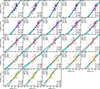 |
Fig. E.2. MHI, R25 versus monochromatic luminosities. See the caption of Fig. E.1. |
| In the text | |
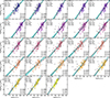 |
Fig. E.3. Mgas,R25 versus monochromatic luminosities. See the caption of Fig. E.1. |
| In the text | |
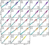 |
Fig. E.4. Mdust versus monochromatic luminosities. See the caption of Fig. E.1. |
| In the text | |
Current usage metrics show cumulative count of Article Views (full-text article views including HTML views, PDF and ePub downloads, according to the available data) and Abstracts Views on Vision4Press platform.
Data correspond to usage on the plateform after 2015. The current usage metrics is available 48-96 hours after online publication and is updated daily on week days.
Initial download of the metrics may take a while.