| Issue |
A&A
Volume 699, July 2025
|
|
|---|---|---|
| Article Number | A293 | |
| Number of page(s) | 21 | |
| Section | Galactic structure, stellar clusters and populations | |
| DOI | https://doi.org/10.1051/0004-6361/202553951 | |
| Published online | 16 July 2025 | |
Reconstructing the Milky Way chemical map with the galactic chemical evolution tool OMEGA+ from SDSS-MWM
1
ELTE Eötvös Loránd University, Gothard Astrophysical Observatory,
9700
Szombathely,
Szent Imre H. st. 112,
Hungary
2
ELTE Eötvös Loránd University, Institute of Physics and Astronomy,
Budapest
1117,
Pázmány Péter sétány 1/A,
Hungary
3
MTA-ELTE Lendület “Momentum” Milky Way Research Group,
Hungary
4
Konkoly Observatory, HUN-REN CSFK/RCAES,
Konkoly Thege Miklós út 15–17,
1121
Budapest,
Hungary
5
The Oskar Klein Centre, Department of Astronomy, Stockholm University, AlbaNova,
10691
Stockholm,
Sweden
6
CSFK HUN-REN, MTA Centre of Excellence, Budapest,
Konkoly Thege Miklós út 15–17.,
1121
Budapest,
Hungary
7
E. A. Milne Centre for Astrophysics, University of Hull,
Cottingham Road,
Kingston upon Hull,
HU6 7RX,
UK
8
NuGrid Collaboration, http://nugridstars.org
9
Center for Astrophysics and Space Astronomy, Department of Astrophysical and Planetary Sciences, University of Colorado,
389 UCB,
Boulder,
CO
80309-0389,
USA
10
Departamento de Física, Universidade Federal de Sergipe, Av. Marcelo Deda Chagas, S/N,
49107-230
São Cristóvão,
SE,
Brazil
11
School of Physics and Astronomy, Monash University,
VIC 3800,
Australia
★ Corresponding author.
Received:
29
January
2025
Accepted:
29
May
2025
Context. Although current observations indicate that there are two distinct sequences of disk stars in the [α/M] versus [M/H] parameter space, further complexity is evident in the chemical makeup of the Milky Way and consequently suggests a complicated evolutionary history.
Aims. We developed two-infall galactic chemical evolution (GCE) models consistent with the Galactic chemical map.
Methods. We obtained new GCE models simulating the chemical evolution of the Milky Way, as constrained by a golden sample of 394 000 stellar abundances of the Milky Way Mapper survey from data release 19 of SDSS-V. The separation between the chemical thin and thick disks was defined using [Mg/M]. We used the chemical evolution environment OMEGA+ combined with Levenberg-Marquardt (LM) and bootstrapping algorithms for the optimization and error estimation. We simulated the entire Galactic disk and considered six galactocentric regions, allowing for a more detailed analysis of the formation of the inner, middle, and outer Galaxy. We investigated the evolution of α, odd-Z, and iron-peak elements, covering 15 species altogether.
Results. The chemical thin and thick disks are separated by Mg observations, which the other α-elements show similar trends with, while odd-Z species demonstrate different patterns as functions of metallicity. In the inner Galactic disk regions, the locus of the low-Mg sequence is gradually shifted toward higher metallicity, while the high-Mg phase is less populated. The best-fit GCE models show a well-defined peak in the rate of the infalling matter as a function of the Galactic age, confirming a merger event about 10 Gyr ago. We show that the timescale of gas accretion, the exact time of the second infall and the ratio between the surface mass densities associated with the second infall event and the formation event vary with the distance from the Galactic center. According to the models, the disk was assembled within a timescale of (0.32±0.02) Gyr during a primary formation phase, followed by an increasing accretion rate over a (0.55±0.06) Gyr-timescale and a relaxation phase that lasted (2.86±0.70) Gyr, with a second peak seen for the infall rate at (4.13±0.19) Gyr.
Conclusions. Our best Galaxy evolution models are consistent with an inside-out formation scenario of the Milky Way disk and in agreement with the findings of recent chemodynamical simulations.
Key words: Galaxy: abundances / Galaxy: evolution / Galaxy: formation / Galaxy: fundamental parameters / Galaxy: general
© The Authors 2025
 Open Access article, published by EDP Sciences, under the terms of the Creative Commons Attribution License (https://creativecommons.org/licenses/by/4.0), which permits unrestricted use, distribution, and reproduction in any medium, provided the original work is properly cited.
This article is published in open access under the Subscribe to Open model. Subscribe to A&A to support open access publication.
1 Introduction
Milky Way (MW) stars of the Galactic plane form a dichotomy in the metallicity versus elemental abundance ratio parameter space, as first discussed by McWilliam (1997) and also by Fuhrmann (1998). The α-elements such as O, Mg, S, Si, Ca, and Ti are mainly produced by massive stars and are therefore of essential importance in distinguishing two populations of stars. The so-called high-α (rich in α-elements) sequence forms the thick disk (Gilmore & Reid 1983), while the thin disk consists of the low-α stellar population. These are often referred to as “low-Ia” and “high-Ia”, respectively, because thin disk stars are generally richer in iron, produced primarily by SNe type Ia. These sequences are also separated kinematically (Gaia Collaboration 2018). The study by Silva Aguirre et al. (2018) demonstrated that the two sequences are characterized by two different ages: the high-α and low-α sequences peak at ~11 Gyr and ~2 Gyr.
A review of the recent semi-numerical galactic chemical evolution (GCE) model results for the MW can be found in Matteucci (2021). The first comprehensive analytical model assumed the instantaneous recycling approximation, which neglects the stellar lifetimes above 1 M⊙ (Tinsley 1980). Other pioneering analytical studies, such as those of Pagel & Tautvaisiene (1995) and Pagel & Tautvaisiene (1997), have investigated the evolution of primary elements in the Galactic disk and in the solar neighborhood. There are many approaches to GCE modeling including serial, parallel, stochastic, and stellar accretion approaches, which we summarize here. First, the halo, thick and thin disks were considered to have formed after one another during one continuous gas infall event (e.g., Chiosi 1980; Boissier & Prantzos 1999). Studies extending this serial approach assumed instead two independent, but sequential accretion episodes (Chiappini et al. 1997). This classical two-infall model assumes that the halo and thick disk formed during the first peak of infall rate, while the thin disk assembled on a longer timescale, reproducing the abundance patterns of the thick- and thin-disk stars, and a gap in the SFR between the two phases sequentially. In such models, we have defined tmax as the time for the maximum infall onto the thin disk, and τ1 and τ2 as the characteristic timescales for gas accretion during the formation of the halo-thick disk and the thin disk.
According to the parallel approach, the gas accretion starts at the same time and occurs in parallel, but at different rates for each infall episode (e.g., Pardi et al. 1995; Grisoni et al. 2017). The stochastic approach was motivated by the large scatter of the chemical abundances of neutron-capture elements for halo stars at low metallicities ([Fe/H] ≲ −3 dex). This scatter reflects that the pollution by a single SNe was not efficiently mixed. The stochastic approach is often applied to the stellar halo (e.g., Cescutti 2008). Finally, the assumption of the stellar accretion means that the Galactic halo accreted stars from the dwarf satellite galaxies of the MW Prantzos (e.g., 2008). This concept was presented by Searle & Zinn (1978), who suggested that the building blocks of the outer halo hierarchically originated from fragments of (dwarf) galaxies over a long timescale.
The inside-out mechanism means that the disk forms by gas accretion much faster in the inner than in the outer disk regions, thereby creating a gradient in the SFR and the [α/M] ratios (Larson 1976; Cole et al. 2000; Bergemann et al. 2014). This approach of formation has been widely adopted to reproduce the observed abundance gradients within the MW (e.g., Spitoni et al. 2015; Palla et al. 2020). For example, in their serial approach, Chiappini et al. (1997) determined tmax = 1 Gyr for an early second infall (while τ1 = 0.8 Gyr for the halo+thick disk) and a significantly longer τ2 = 7–8 Gyr thin disk assembly time at the solar vicinity.
Spitoni et al. (2019) suggested a revised two-infall model, with the second infall occurring with a delay of ~4.3 Gyr relative to the formation, to reproduce the observed bimodality and the stellar ages. The gap in star formation predicts a loop in the model curves describing the abundance ratios in the solar vicinity (see later in e.g., Fig. 5) and a decrease in tmax produces a loop starting at lower metallicities (Spitoni et al. 2019). The tmax delay was also analyzed by Vincenzo et al. (2019), proposing that a massive satellite called Gaia-Sausage/Enceladus (Helmi et al. 2018) was accreted by the Galaxy during a major merger event. This scenario of a high-impact merger is in agreement with Chaplin et al. (2020) who showed that the metal-poor, high-α star ν Indi was originally a member of the halo, which made it possible to infer that the earliest time when the merger could have begun was 11.6 Gyr ago.
Migration has been proposed as a complementary to two-infall (e.g., Spitoni et al. 2015) or alternative (e.g., Buck 2020; Sharma et al. 2021; Prantzos et al. 2023) solution to explain the low-α and the high-α sequences. It has been shown by Roškar et al. (2008) that resonant scattering at corotation may migrate stars outward while the gas moves inward. The study from Vincenzo & Kobayashi (2020) showed that stellar migration involves old metal-rich stars and occurs more outward than inward. However, Khoperskov et al. (2020) concluded that it has a negligible effect on the [α/M] versus [M/H] relation.
Chemical enrichment in galaxies is traced by the chemical elements produced by stars of different initial masses, when part of their mass is redistributed to the ISM when they die. Chemical elements have different contributions from exploding massive stars, neutron star mergers, SNe type Ia, or dying low-mass stars (Kobayashi et al. 2020). The evolution of elemental ratios is also driven by phenomena such as galactic winds, star formation history (SFH), and gas inflows and outflows. For such GCE studies, obtaining significant high-resolution spectroscopic data of stellar atmospheres is crucial.
The Sloan Digital Sky Survey is a ground-based panoptic program now operating in its fifth phase (Kollmeier et al., in prep.), which is performing multi-epoch optical and infrared observations across the entire sky (Gunn et al. 2006). One of its projects, the Milky Way Mapper survey (MWM, Kollmeier et al., in prep.) is the successor of Apache Point Observatory Galactic Evolution Experiment (APOGEE, Majewski et al. 2017). It will obtain high-precision spectroscopic data of five million objects throughout the sky by 2027 to provide a dense and contiguous stellar map while mainly focusing on low Galactic latitudes. The survey employs both optical and near-infrared spectroscopy performed with BOSS (Smee et al. 2013) low-resolution (R ~ 2000) and APOGEE (Wilson et al. 2019; Bowen & Vaughan 1973) high-resolution (R ~ 22 500) instruments, respectively. Stellar parameters and atmospheric chemical composition of each star involved in the program were derived from the high signal-to-noise (S/N) spectra.
In this work, we performed two-infall GCE models intending to reproduce the chemical maps of the MW drawn by private data of SDSS-V MWM, published in its first data release (DR19, Meszaros et al., 2025, under rev., hereinafter M25). This study covers the evolution of α, odd-Z and iron-peak elements, 15 species altogether. By dividing the Galaxy into six regions, we analyze the solar vicinity, the inner and outer regions of the thick- and thin-disk system. The motivation raised from the work of Spitoni et al. (2021, hereinafter S21) following up on their prior studies (Spitoni et al. 2017b, 2019), but spatially dividing the MW into twice as many galactocentric regions. We used the One-zone Model for the Evolution of Galaxies (OMEGA, Côté et al. 2017a) and its extension the Two-zone Model for the Evolution of Galaxies (OMEGA+, Côté et al. 2018). The OMEGA+ code has been designed to run GCE simulations1. For previous GCE studies using these tools, we refer to Pignatari et al. (2023) for the GCE of the solar neighborhood, Liang et al. (2023) for assessing stellar yields, and Côté et al. (2019) for probing the origin of r-process elements or dwarf galaxies (Côté et al. 2017a).
2 Target and data selection
2.1 The Milky Way Mapper DR19 sample
As part of SDSS-V, one of the innovations of MWM is its new automated pipeline called Astra (Casey et al., in prep.) that derives stellar atmospheric parameters for the new MWM and also for the old APOGEE observations by reanalyzing those measurements. Astra is capable of running multiple algorithms developed to derive abundances, including the APOGEE Stellar Parameters and Chemical Abundance Pipeline (ASPCAP; García Pérez et al. 2016), which relies on the FERRE2 multi-dimensional χ2 optimization code (Allende Prieto et al. 2006). Individual abundances of elements that are used in this paper are derived in the second phase of ASPCAP by fixing the main atmospheric parameters obtained in the first phase, while fitting the wavelength windows sensitive to only the particular element. We note that NLTE effects were not taken into account in the spectral grid in DR19 (M25).
The first data release of MWM is publicly available online3, and contains spectroscopic, photometric, and astrometric information of 1 095 480 individual stars, from which we extracted the effective temperature (Teff), surface gravity (log g), metallicity ([M/H]), and calibrated abundance of the relevant element X ([X/H], where X = {α, O, Mg, Si, S, Ca, Ti, Na, Al, K, V, Cr, Mn, Co, and Ni}), and equatorial coordinates (RA, Dec) along with parallax (p), as well as the quality flags. We note that the α-capture elements considered in ASPCAP are the following: O, Mg, Si, S, Ca, and Ti. Practically, the [α/M] abundance value reflects the O, Mg, and Si because these have the strongest lines, while S, Ca, and Ti have lower weights within the fitting of the α-dimension (M25). The oxygen abundance is derived from OH molecular lines in the H-band, that is sensitive to Teff, although reliable between 3500 and 6000 K (M25). The atmospheric parameters Teff and log g are calibrated to the photometric scale based on the infrared flux method and to asteroseismic surface gravities, respectively. For the individual abundances, zero-point offsets are applied using the solar neighborhood and solar metallicity red giant branch (RGB) stars. These calibrations and an exhaustive assessment of the overall uncertainties are explained in detail by M25. The reported values of the overall precision of Teff, log g, metallicity, and individual chemical abundance ratios for the giants are 50–70 K, 0.05–0.33 dex, 0.03 dex, and below 0.15 dex for most of the elements (except for e.g., vanadium), respectively.
We use the customary scale of logarithmic abundances defined as A(X) = log(NX/NH) + A(H), where A(H) ≡ 12 and NX is the number of atoms of element X per unit volume in the atmosphere. The abundance ratio is defined relative to the chemical composition of the Sun:
![$\[[\mathrm{X} / \mathrm{H}]=\log \left(n_X / n_H\right)_{\star}-\log \left(n_X / n_H\right)_{\odot}.\]$](/articles/aa/full_html/2025/07/aa53951-25/aa53951-25-eq1.png) (1)
(1)
Elemental abundances are usually determined relative either to hydrogen [X/H] or iron [X/M], and the conversion between them is given by
![$\[[\mathrm{X} / \mathrm{H}]=[\mathrm{X} / \mathrm{M}]+[\mathrm{M} / \mathrm{H}].\]$](/articles/aa/full_html/2025/07/aa53951-25/aa53951-25-eq2.png)
Both the overall metallicity [M/H] and the iron abundance [Fe/H] are published in DR19 (M25). While [M/H] is determined by fitting the entire H-band spectrum as an overall scaling factor of all the metal abundances with a solar abundance pattern, [Fe/H] is derived in the second stage of the fit in wavelength windows that are sensitive to Fe I lines. The two metallicity indicators generally provide the same values within the expected uncertainties (M25). The median difference between iron and all metal abundances is 0.01 dex with a scatter of only 0.03 dex. We refer to [M/H] as metallicity throughout this study.
2.2 Target selection
2.2.1 Quality cuts
This section discusses our selection criteria to obtain a reliable parameter space covering the Galactic disk. We opted out stars that are marked with the quality control flag_bad by the ASPCAP pipeline, as well as if one of the atmospheric parameters (Teff, log g, [M/H], [Mg/M], [α/M]) is missing. Moreover, we applied a S/N cut of 50 so that we could use the most reliable parameter space proposed by MWM (M25). As recommended by M25, we also eliminated stars having Teff < 4250 K and [C/M] > 0.1 dex. The reason is that this carbon-rich cool group cannot be accurately fitted by ASPCAP, regardless of their surface gravity. The [C/M] abundance affects all spectral regions as it is determined from the global fit of the spectra and kept fixed in the stages of determining the individual abundances.
2.2.2 Atmospheric parameter selection
For the main atmospheric parameters, we followed the cuts suggested by Hayden et al. (2015), therefore, only stars with Teff ∈ [3500 K; 5500 K], and log g ∈ [1.0 dex; 3.8 dex] were retained in the sample. This Teff–log g range contains RGB and red clump stars within the most reliable parameter range of MWM, excluding main sequence stars, which have less reliable abundances than giants in DR19 (M25).
2.2.3 Spatial selection
Here, we attempt to focus on the evolution of the Galactic disk. Therefore, we selected stars from this region of the MW according to their Galactocentric distances, R, and vertical heights, Z. To perform the conversion from the (RA, Dec) equatorial coordinates and the Gaia DR3 parallax p published4 in MWM DR19 to the (R, ϕ, Z) cylindrical galactocentric frame, we used the astropy package (Astropy Collaboration 2022). This coordinate transformation assumes the Galactocentric distance from the Sun to the Galactic center R⊙ = 8.122 kpc and its location above the Galactic mid-plane Z⊙ = 20.8 pc (GRAVITY Collaboration 2019). Similarly to, for instance, the approach described in Griffith et al. (2021), the selected stars are characterized by distances from the center and from the Galactic mid-plane of 3 kpc ≤ R ≤ 15 kpc and |Z| < 5 kpc, respectively. This is an extended range of the vertical distance of |Z| < 2 kpc used by Hayden et al. (2015).
This study does not consider the innermost central region of R < 3 kpc, as the Galactic bulge characteristics are dominant there, and a different GCE setup is required for this central component. However, recent works (e.g., Queiroz et al. 2020) based on APOGEE DR16 data confirm that a disk-like, bimodal [α/M] versus [M/H] abundance distribution is also observed in the Galactic bulge. It was reported in Queiroz et al. (2020) that contamination caused by varying the definition for the spatial coverage of the bulge, within a range of 2–6 kpc, does not account for significant changes in the observed bimodal disk-like distribution. Here, we confirm that MWM DR19 stars with Galactocentric distances selected from the range of R = 2–6 kpc represent an almost identical distribution in the [Mg/M] versus [M/H] abundance ratio space as those enclosed in a region of R = 3–6 kpc.
In addition, stars with a high probability of being globular cluster (GC) members were also removed from the sample. Our source to perform this identification was the SDSS-IV/APOGEE DR17 (Abdurro’uf et al. 2022) value-added catalog (VAC) of Galactic GC stars, which contains membership information for 7732 observations (6422 unique stars) in 72 GCs in the MW (Schiavon et al. 2024). To achieve completeness in spatial filtering, we deleted stars still marked as likely GC or dwarf galaxy (such as ωCen) members. Under the label of sdss4_apogee_member_flags, a bit is set if a given target meets several membership criteria5. In the VAC, under the relevant flag label, candidate members are assigned based on sky position, proper motion, and radial velocity.
The [M/H] versus [α/M] distribution for the Galaxy of the original DR19 data set and the sample after our cuts are shown in Fig. 1. We note that the separation of the low-Mg and high-Mg populations became sharper and less scattered after applying the cuts described above, while the artifacts (and synthetic nodulations) have disappeared. While the original DR19 data set contains 1 095 480 stars, we retained 393 743 objects to use in the GCE models after applying our selection.
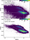 |
Fig. 1 Observed stellar [α/M] vs. [M/H] abundance ratios from MWM DR19 (Meszaros et al., in prep.). The top panel shows a density plot for all the stars published, while the disk stars involved in the quality disk sample at the galactocentric regions 3 kpc ≤ R ≤ 15 kpc are depicted in the bottom panel. Color-coding of the bins starts from two, and gray squares represent bins containing a single star. The total number of stars is denoted by N. |
2.3 Data description
In this work, we analyzed the Galactic disk between R = 3 kpc and 15 kpc, dividing the sample into the concentric annular rings in steps of ΔR = 2 kpc. After applying the selection criteria described in Sect. 2.2, we created chemical maps of the Galactic disk for the total α-elemental abundance, and for the other 14 single elemental species: Mg, O, Si, S, Ca, Ti, Na, Al, K, V, Cr, Mn, Co, and Ni. The separation between the populations is determined by two linear functions on the Mg abundance distribution of the MW. We note that Hayden et al. (2015) and Weinberg et al. (2019) performed a similar division on the same [Mg/M] versus [M/H] parameter plane. The boundary line is a decreasing linear function at metallicities below zero and a constant above zero, as described by
![$\[[\mathrm{Mg} / \mathrm{M}]= \begin{cases}-0.17 \cdot[\mathrm{M} / \mathrm{H}]+0.12 \operatorname{dex}, & {[\mathrm{M} / \mathrm{H}] \leq 0}, \\ 0.12 \operatorname{dex}, & {[\mathrm{M} / \mathrm{H}]>0}.\end{cases}\]$](/articles/aa/full_html/2025/07/aa53951-25/aa53951-25-eq3.png) (2)
(2)
We determined the slope of the line regression by first dividing the distribution into 30 metallicity bins between −1 dex < [M/H] < 0 dex, followed by fitting the Mg distribution in each [M/H] bin (vertical projection in the parameter-plane) with the sum of two Gaussians, then we fit a linear function on the minimum values of these two-peak functions. The resulting linear function is denoted by a solid line in the Mg panel of Fig. 2. The high-Mg sequence is defined between −1.0 dex < [M/H] < 0.0 dex, whereas the low-Mg phase starts at [M/H] = −0.6 dex and ranges up to the metallicity of [M/H] = 0.5 dex. Outside of these boundaries, the [Mg/M] distributions do not display any relevance to the sequences and/or contain only few observations.
After performing the separation according to Eq. (2), the median values of the resulting two sets of stars were considered as the locus of the high-Mg and low-Mg populations. The thin and thick disks are also aptly separated by the other elements in Fig. 2, which displays the characteristic sequences defined by Mg. While most elements show similar trends to Mg, the abundance trends of odd-Z elements such as Co, Mn, and V are noticeably discrepant, exhibiting a completely different pattern as function of metallicity. We note that Ti and V abundances derived from APOGEE data are known to be challenging to measure precisely in red giant stars, primarily due to the weakness of their spectral lines, as discussed by Souto et al. (2016, 2018).
Hereinafter, the “global sample” refers to all stars spanning the range of 3 kpc ≤ R ≤ 15 kpc, while the six 2-kpc-wide, distinct regions make up the inner zone (first and second regions covering 3 kpc ≤ R < 7 kpc), the middle zone (third and fourth regions covering 7 kpc ≤ R < 11 kpc), and the outer zone (fifth and sixth regions, covering 11 kpc ≤ R ≤ 15 kpc). For the exact numbers of the subsets, we refer to Fig. 3 and Table 3. The highest number of observed stars appears in the third region, which includes the solar neighborhood, while the sixth region contains the least measurements The chemical maps in the concentric annuluses are shown in Fig. 3. The two populations visible in the [Mg/M] versus [M/H] relation have variable trends with the radius, as reported by Hayden et al. (2015) and Queiroz et al. (2020) from the APOGEE data. The average [Mg/M] values of the thick disk remain roughly the same between the regions; therefore the expression of Eq. (2) used to separate the thin and thick disks can be applied for all regions uniformly.
The low-Mg population shows lower and upper boundaries at increasingly lower metallicity toward the outer disk, while the metallicity range of the high-Mg population covers the −0.85 dex < [M/H] < −0.10 dex range across all regions. In other words, the locus of the low-Mg sequence is shifted toward higher metallicity in the inner regions. It is also clear from Fig. 3 that stars at the outer edge of the Galaxy (bottom panel, sixth region) preferentially populate the low-Mg sequence in the [Mg/M] versus [M/H] space and few stars are located in the highMg population. More specifically, the ratio between the number of low-Mg and high-Mg stars increases when considering the outer Galactic regions.
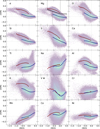 |
Fig. 2 Chemical map of the Galaxy observed by MWM. The [X/M] vs. [M/H] relations are shown for the combined α-elemental ratio as well as the single elements from Mg to Ni for the global disk sample. Red and blue curves represent the median trends of the high- and low-Mg stars separated based on their Mg abundance. This separation and the metallicity boundaries of the thick and thin disk stars are indicated by the black solid and dashed lines in the panel of Mg. Note: ⊗ drives caution to V because of the high observational uncertainty. |
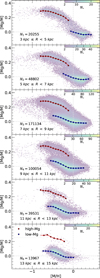 |
Fig. 3 Observed stellar [Mg/M] vs. [M/H] abundance ratios from MWM DR19 (Meszaros et al., in prep.) for the six bins of different Galactocentric distances considered here. The regions plotted from the top are all 2-kpc-wide, and are centered at R1 = 4 kpc, R2 = 6 kpc, R3 = 8 kpc, R4 = 10 kpc, R5 = 12 kpc, and R6 = 14 kpc, respectively. The sample size in the i-th region is denoted by Ni. Red and blue squares represent the binned distributions of the high-Mg and low-Mg sequences, respectively. Details on the data selection are reported in the text. |
3 The GCE model for the disk and OMEGA+
In this section, we present the main properties of our GCE simulation presented here, confirming and expanding the main results by Spitoni et al. (2019, 2021). We describe how the galaxy evolution code works, along with the modifications to the original OMEGA/OMEGA+ software.
3.1 Fundamental assumptions of GCE
3.1.1 Distribution of individual stars
To describe the dN number of stars in the interval [m, m + dm], we adopted Kroupa (2001) for the initial mass function:
![$\[d N=\xi_0 m^{-a(m)} d m,\]$](/articles/aa/full_html/2025/07/aa53951-25/aa53951-25-eq4.png) (3)
(3)
which has a power-law index of a1 = 1.3 over the range of stellar masses 0.08 ≤ m/M⊙ < 0.5 (and a2 = 2.3 otherwise). The ξ0 normalization constant was obtained from the condition of ![$\[\int_{M_{\text {min }}}^{M_{\text {max }}} m \xi(m) d m=1\]$](/articles/aa/full_html/2025/07/aa53951-25/aa53951-25-eq5.png) . Our prior tests suggested that the characteristic shape of the model curve in the [M/H]–[Mg/M] parameter plane was obtained with these choices of a1 and a2. We set the lower and upper mass limits of the IMF to 0.08 M⊙ and 130 M⊙, respectively.
. Our prior tests suggested that the characteristic shape of the model curve in the [M/H]–[Mg/M] parameter plane was obtained with these choices of a1 and a2. We set the lower and upper mass limits of the IMF to 0.08 M⊙ and 130 M⊙, respectively.
The age of each source is crucial to defining the timeline for mixing the metals in the ISM. On the other hand, massive stars effectively release metals instantaneously, when the simulation time step is larger than their lifetimes. The number of explosions per stellar mass formed can be easily calculated from the IMF within the pre-defined mass range for massive stars of 9 M⊙ to 30 M⊙. Above the upper mass limit, we assume stars directly collapse into black holes (Ebinger et al. 2020; Boccioli & Fragione 2024). We acknowledge that this assumption may could prove incorrect when investigated in detail, as neutrino driven models of core-collapse supernovae (CCSNe, SNe type II) produce complex mass landscapes of black hole formation and successful explosions (e.g., Ugliano et al. 2012; Pejcha & Thompson 2015). Conversely, progenitors of SNe Ia have longer lifetimes within the OMEGA+ simulations. As proposed by Greggio (2005), the occurrence rate of SNe Ia for a simple stellar population (stars born at the same time and with the same chemical composition, SSP) can be calculated as the product of the SFR and a so-called delay-time distribution (DTD) function that describes the probability distribution of the explosion times. In this function, the fraction of white dwarfs is calculated from the lifetime of intermediate-mass stars and the IMF. The DTD(t) function is normalized over the stellar lifetimes to describe the sequence of SNIa explosions. Therefore, in the simulations, we applied the exponential approach introduced by Pritchet et al. (2008) and discussed by Wiersma et al. (2009), where the decreasing DTD(t) is written in the form of
![$\[\mathrm{DTD} \propto e^{-t / t_\beta},\]$](/articles/aa/full_html/2025/07/aa53951-25/aa53951-25-eq6.png)
where tβ determines the characteristic decay time of the DTD. We set tβ = 2 · 109 years, as used by, for instance, Wiersma et al. (2009). The number of SNe Ia per stellar mass formed in a simple stellar population is assumed to be NIa/M⊙ = 0.0020 in our work, which was also proposed by Maoz & Mannucci (2012) based on their examination of SN rate compilations.
3.1.2 The chemical evolution model for the Milky Way
The time-delay model explains the behavior of the combined α elemental (O, Mg, S, Si, Ca) abundances because in the early phases of Galactic evolution, these elements are only produced by massive stars characterized by short lifetimes, thereby resulting in an average overabundance at low metallicity ([M/H] < −1 dex). Later SNe type Ia started to contribute with a time delay relative to CCSNe and produced the bulk of the iron. As SNe type Ia begin to contribute, the [α/M] ratios starts to decrease with time, until they reached the solar value. The main equation of chemical evolution describes the surface mass density of each element in the interstellar medium (ISM) at a given time. This may be solved only numerically, as the term involving the SFR and IMF grows with the integration time (see e.g., Matteucci & Tornambe 1985; Matteucci & Greggio 1986; Francois 1986).
For the semi-analytical calculations, we used a modified version of OMEGA+ (Côté et al. 2018), that is built on OMEGA (Côté et al. 2017a). In the framework of OMEGA+, the simulated system consists of a cold gas reservoir, which is a star-forming region, and contains the stellar population of the Galaxy. This volume is surrounded by a hot gas reservoir (as the outer zone) filling the dark matter halo. This is considered to be the circumgalactic medium (CGM) from which the inflows happen. OMEGA simulates the inner star-forming region, then the rates of galactic inflow and outflow, and star formation are controlled by OMEGA+.
The accretion from the external zone into the CGM is generally called the circumgalactic inflow and is assumed to have a primordial chemical composition. At the beginning of the simulation, the Galaxy is considered primordial. Then, the overall gas circulation (similarly to the evolution of the mass of the cold gas reservoir) is tracked as the core of the calculations. The metallicity of the galactic gas is diluted by inflows from the CGM, stellar ejecta contributes to the mass-loss rate and the star formation rate (SFR) drives how much metal is ejected into the CGM. In each time step, a simple stellar population is created that drives the galactic outflow, also resulting in a decrease of the inner metallicity (Côté et al. 2018).
In the default setup (Côté et al. 2018), the rate of the infalling matter to the galaxy from CGM is constant. We discuss in Sect. 3.2 that the two-infall scenario instead requires an exponentially driven two-peak inflow rate; therefore, we customized this function with free parameters during the fitting.
3.2 Implementations to OMEGA+
To describe the relationship between the SFR and surface mass density of the gas, we adopted the Schmidt–Kennicutt law:
![$\[\dot{M}_{\star}(t)=\nu \sigma^k(t),\]$](/articles/aa/full_html/2025/07/aa53951-25/aa53951-25-eq7.png) (4)
(4)
where ν is the star formation efficiency (SFE), which shows the fraction of the gas mass turned into newly forming stars per unit time, and k = 1.5 (Schmidt 1959; Larson 1988, 1992; Kennicutt 1998). We set ν = 0.022 for the simulations.
Within the classical double-infall approaches (e.g., S21), the inflow rate describing the merger episode is assumed to be zero until a certain time (tmax) when the inflow peak is introduced instantaneously by an exponentially decreasing function with a characteristic accretion time τ. To fine-tune our two-infall scenario, we introduce rising phases of the surface mass density arriving at the Galactic disk per unit time ![$\[(\dot{\sigma}(t))\]$](/articles/aa/full_html/2025/07/aa53951-25/aa53951-25-eq8.png) :
:
![$\[\begin{aligned}\dot{\sigma}(t):= & \frac{\dot{M}_{\text {in }}(t)}{A}=\sum_{k=\{1,2\}} \dot{\sigma}_{k, 0}\left[\theta\left(t_{\max, k}-t\right) e^{\left(t-t_{\max, k}\right) / \tau_k^{\prime}}\right. \\& \left.+\theta\left(t-t_{\max, k}\right) e^{-\left(t-t_{\max, k}\right) / \tau_k}\right],\end{aligned}\]$](/articles/aa/full_html/2025/07/aa53951-25/aa53951-25-eq9.png) (5)
(5)
where A = (R2 − r2) π is the surface of the Galactic annulus bounded by r and R, the ![$\[\dot{\sigma}_{k, 0}\]$](/articles/aa/full_html/2025/07/aa53951-25/aa53951-25-eq10.png) normalization factors are the rates of the surface mass densities related to the k-th infall event, and θ(t − tmax) is the unit step function which has a value of zero if t < tmax and one otherwise. We implemented this form of inflow rate in OMEGA+. It provides infalling peaks that have an exponentially increasing phase and a decreasing branch with characteristic times
normalization factors are the rates of the surface mass densities related to the k-th infall event, and θ(t − tmax) is the unit step function which has a value of zero if t < tmax and one otherwise. We implemented this form of inflow rate in OMEGA+. It provides infalling peaks that have an exponentially increasing phase and a decreasing branch with characteristic times ![$\[\tau_{k}^{\prime}\]$](/articles/aa/full_html/2025/07/aa53951-25/aa53951-25-eq11.png) and τk, respectively, both assumed as free parameters. More specifically,
and τk, respectively, both assumed as free parameters. More specifically, ![$\[\tau_{1}^{\prime}\]$](/articles/aa/full_html/2025/07/aa53951-25/aa53951-25-eq12.png) corresponds to an intense infall at the beginning of galaxy formation. It has a fixed value of
corresponds to an intense infall at the beginning of galaxy formation. It has a fixed value of ![$\[\tau_{1}^{\prime}=0.05\]$](/articles/aa/full_html/2025/07/aa53951-25/aa53951-25-eq13.png) Gyr, while the other accretion parameters (
Gyr, while the other accretion parameters (![$\[\tau_{2}^{\prime} \equiv \tau_{\mathrm{up}}\]$](/articles/aa/full_html/2025/07/aa53951-25/aa53951-25-eq14.png) , τ1, and τ2) are varied within the simulations. The time of the first infall is at the birth of the Galaxy, and for numerical reasons, it is fixed to be tmax,1 = 0.1 Gyr, and the tmax,2 ≡ tmax delay duration between the two infall episodes is also a free parameter.
, τ1, and τ2) are varied within the simulations. The time of the first infall is at the birth of the Galaxy, and for numerical reasons, it is fixed to be tmax,1 = 0.1 Gyr, and the tmax,2 ≡ tmax delay duration between the two infall episodes is also a free parameter.
The ![$\[\dot{\sigma}_{k, 0}\]$](/articles/aa/full_html/2025/07/aa53951-25/aa53951-25-eq15.png) normalization factors related to the first and second infalls in Eq. (5) are derived by the following considerations. The present-day surface mass density is the integral of Eq. (5) over the entire time duration of the evolution from t = 0 to t = tG:
normalization factors related to the first and second infalls in Eq. (5) are derived by the following considerations. The present-day surface mass density is the integral of Eq. (5) over the entire time duration of the evolution from t = 0 to t = tG:
![$\[\begin{aligned}\sigma_k\left(t_{\mathrm{G}}\right) & =\int_0^{t_G} \dot{\sigma}_k(t) d t \\& =\dot{\sigma}_{k, 0}\left(\int_0^{t_{\max, \mathrm{k}}} e^{\left(t-t_{\max, \mathrm{k}}\right) / \tau_k^{\prime}} d t+\int_{t_{\max, \mathrm{k}}}^{t_G} e^{-\left(t-t_{\max, \mathrm{k}}\right) / \tau_k} d t\right) \\& =\dot{\sigma}_{k, 0}\left(\tau_k^{\prime}-\tau_k^{\prime} e^{-t_{\max, \mathrm{k}} / \tau_k^{\prime}}+\tau_k-\tau_k e^{\left(t_{\max, \mathrm{k}}-t_{\mathrm{G}}\right) / \tau_k}\right),\end{aligned}\]$](/articles/aa/full_html/2025/07/aa53951-25/aa53951-25-eq16.png) (6)
(6)
where tG is the entire galactic lifetime. Thus, the normalization factor for each infall episode is determined as
![$\[\dot{\sigma}_{k, 0}=\frac{\sigma_k\left(t_G\right)}{\tau_k^{\prime}\left(1-e^{-t_{\max, \mathrm{k}} / \tau_k^{\prime}}\right)+\tau_k\left(1-e^{\left(t_{\max, \mathrm{k}}-t_G\right) / \tau_k}\right)}.\]$](/articles/aa/full_html/2025/07/aa53951-25/aa53951-25-eq17.png) (7)
(7)
Here, σk (tG) ≡ σk is the present-day surface mass density related to the k th infall episode. Here the sum and the ratio of the surface densities σtot and σ2/σ1 are the free parameters to optimize, where σ1 and σ2 can be obtained by σ2 = σtot/(1 + σ2/σ1) and σ1 = σtot − σ2.
Therefore, the inflow rate is defined by the product of the surface mass density infalling per unit time and the 2D surface of the projection of the annular disk in the (R − ϕ) plane (or on the direction perpendicular to the direction of Z-axis indicating Galactic height). Furthermore, according to Eq. (5), we can reformulate the global inflow rate as
![$\[\begin{aligned}\dot{M}_{\text {in }}(t)= & \left(R^2-r^2\right) \pi \sum_{k=\{1,2\}} \dot{\sigma}_{k, 0}\left[\theta\left(t_{\max, k}-t\right) e^{\left(t_{\max, k}-t\right) / \tau_k^{\prime}}\right. \\& \left.+\theta\left(t-t_{\max, k}\right) e^{-\left(t-t_{\max, k}\right) / \tau_k}\right],\end{aligned}\]$](/articles/aa/full_html/2025/07/aa53951-25/aa53951-25-eq18.png) (8)
(8)
where r = 3 kpc and R = 15 kpc are the inner and outer radii of the Galactic disk.
The total present-day surface mass density at the Galactocentric distance R can be described as
![$\[\sigma_{\text {tot }}(R)=\sigma_{\text {tot }, \odot} ~e^{-\left(R-R_{\odot}\right) / R_d},\]$](/articles/aa/full_html/2025/07/aa53951-25/aa53951-25-eq19.png) (9)
(9)
where σtot,⊙ is the total surface density observed in the solar neighborhood, and the scale-length of the disk is Rd = 3.5 kpc (Spitoni et al. 2017a). We introduce the σtot,n partial surface mass densities that are assumed to be constant within each 2-kpc wide region. Assuming that the values of σtot,n are constant within each region but fulfill the criterium of Eq. (9), the ratio between the densities in the neighboring regions is q = σtot,n+1/σtot,n = e−ΔR/Rd, where n = {1; 2; ...; 6}. Supposing that the partial densities are weighted by the powers of this quotient, q, as well as by the area of the relevant annular galactocentric ring, we obtain
![$\[A_n=\pi\left[\left(R_n+\Delta R / 2\right)^2-\left(R_n-\Delta R / 2\right)^2\right]=2 \pi R_n \Delta R,\]$](/articles/aa/full_html/2025/07/aa53951-25/aa53951-25-eq20.png) (10)
(10)
and the nth partial surface mass density in the form of a sequence
![$\[\sigma_{\mathrm{tot}, \mathrm{n}}=\sigma_{\mathrm{tot}, 0}\left[R_1+(n-1) \Delta R\right] ~q^{n-1},\]$](/articles/aa/full_html/2025/07/aa53951-25/aa53951-25-eq21.png) (11)
(11)
where σtot,0 is the inverse normalization coefficient. As the summation of this sequence should return the total fitted value, the σtot,0 factor can be derived by the relation
![$\[\sigma_{\mathrm{tot}, 0}=\frac{\sigma_{\mathrm{tot}}}{\sum_{i=1}^6\left(\left[R_1+(i-1) \Delta R\right] ~q^{i-1}\right)}.\]$](/articles/aa/full_html/2025/07/aa53951-25/aa53951-25-eq22.png) (12)
(12)
Here, the nth partial surface mass density is calculated according to Eq. (11). In the solar neighborhood, the total baryonic mass surface density today is σtot,⊙ = (47.1 ± 3.4) M⊙pc−2 (McKee et al. 2015). Since outflows also happen, the total infalling surface mass density in the solar region (7 kpc ≤ R < 9 kpc) is accepted to result in a different value in the simulations. Also, the surface density σtot,3 represents the average surface density within the Galactic ring centered at 8 kpc.
In summary, the total infalling matter during the simulation is spatially distributed into the regions, and we assume that within the nth region, the regional partial surface mass density, σtot,n is constant along its width of 2 kpc. The values at the centers of the regions (Rn = 4; 6; ...; 14 kpc) follow the exponentially decreasing distribution described by Eq. (9). Each calculated σtot,n is listed in Table 3, and shown in Fig. 9. Due to these implementations, the regions are coupled to each other, since the integral of the global inflow rate function over Galactic age is equal to the sum of the integrals of the partial inflow functions.
At the beginning of the simulation and around the second infall event, GCE quantities (e.g., SFR) change rapidly. Therefore, the first time step is 0.1 Myr long, and until it reaches 50 Myr, a logarithmic scale is used. During the remaining Galactic time, a uniform resolution is applied. We consider the age of the Sun to be 4.57 Gyr (e.g., Boothroyd & Sackmann 2003).
3.3 Nucleosynthetic yield sets
Depending on its initial mass, each star produces unique amounts of the chemical elements, and ejects them in the ISM once its lifetime expires. Stellar yields are computed with detailed nucleosynthesis calculations considering all the main nuclear reactions in stars and supernovae. Theoretical stellar yields are used as input for different GCE models. The mass of a newly formed element k in a star of mass, m, is defined as
![$\[M_{k m}=\int_0^{\tau_m} \dot{M}_{\text {lost }}(t) \cdot\left[X(t, k)-X_o(k)\right] ~d t,\]$](/articles/aa/full_html/2025/07/aa53951-25/aa53951-25-eq23.png) (13)
(13)
where τm is the lifetime of a star of initial mass ![$\[m, \dot{M}_{\text {lost}}\]$](/articles/aa/full_html/2025/07/aa53951-25/aa53951-25-eq24.png) is the mass loss rate of the star (the rate of the mass that is ejected by the star into the ISM) and Xo(k) and X(t, k) are the original and final abundances of the element k, respectively. The stellar yield is given by the fraction of the stellar mass converted into that element: pkm = Mkm/m, where Mkm is the total mass of the newly formed chemical species.
is the mass loss rate of the star (the rate of the mass that is ejected by the star into the ISM) and Xo(k) and X(t, k) are the original and final abundances of the element k, respectively. The stellar yield is given by the fraction of the stellar mass converted into that element: pkm = Mkm/m, where Mkm is the total mass of the newly formed chemical species.
Through the JINA-NuGrid chemical evolution pipeline (Côté et al. 2017b), OMEGA+ has access to NuPyCEE stellar yields library for low-, intermediate-, and high-mass stars (Pignatari et al. 2016; Ritter et al. 2018). The tables provide the stellar yields on a grid that spans over 12 stellar models between 1 and 25 M⊙, and between five metallicities from Z = 0.0001 to 0.02. Beyond these points, stellar yields are interpolated as a function of metallicity and mass.
The initial metallicity of the gas in mass fraction of all stellar ejecta is uniformly set to be Z = 0.001 in this work. We adopted the Cristallo et al. (2015) yield set within the regime up to the asymptotic giant branch. The AGB yields are extracted from FRUITY (Cristallo et al. 2011) and massive star yields from NuGrid (Pignatari et al. 2016), whereas lifetimes for AGB models were taken from NuGrid (Ritter et al. 2018). The minimum mass of SNe type II (Mtrans) sets the transition between intermediate mass and massive stars. We set the value of Mtrans = 9 M⊙, consistent with the that used in literature (8–10 M⊙, Matteucci 2021). The yields of SNe Ia are taken from Iwamoto et al. (1999). For the nucleosynthetic yields of an initial generation of massive metal-free stars (often referred to as population III stars), we adopt Heger & Woosley (2010). We assume that stars with initial masses of 10–100 M⊙ contribute to explosive nucleosynthesis, while those more massive than 100 M⊙ collapse to black holes.
The nucleosynthetic yields for many elements are under or over predicted due to many factors including uncertainties in nuclear reaction rates and atomic cross sections, explosion assumptions, and computational limitations. To correct for these known problems, we introduce multiplication factors, denoted by fX, to the values reported in the yield tables. These correction factors are fit as free parameters in our final GCE models. To demonstrate the necessity of the correction factors, in Fig. 4 we show the global GCE model results for Mg and O without the fX corrections compared to the MWM data. We see that the model severely under-predicts [Mg/M] and slightly under-predicts [O/M] when no yield correction factors are applied. We fit one correction factor per element, and multiply yields from all nucleosynthetic sources by this value.
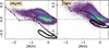 |
Fig. 4 Version of the GCE results for [M/H] versus Mg and O abundance ratios obtained without applying yield correction factors. The other GCE parameters are fixed at the best-fit values found in Sect. 5. |
List of the GCE parameters.
4 Fitting methods
4.1 Determination of the free parameters in the GCE models
The main GCE parameters are listed and defined briefly in Table 1. We categorize the model parameters and the effects of physical processes into four groups based on how we treat them in the fitting method. First, there are effects that we ignore, such as dark matter in the disk, pre-enriched inflows, variation of the SFE and mass-loading factor (η) along the Galactocentric radii, the lifetime of stars above Mtrans, and the effect of radial stellar migration.
Secondly for the GCE simulations, we fix the Mtrans = 9 M⊙ lower boundary of massive stars, and the [0.08, 130] range of initial mass function in solar masses. Consistently with the considerations of Côté et al. (2016), we assume that above the mass of Mth = 30 M⊙ stars do not release any ejecta, but directly collapse into black holes. Therefore, the maximum mass in the IMF affects the total mass of gas locked into stars, but not the ejected yields. In order to test such an assumption, we have made additional GCE simulations using Mth = 100 M⊙ as an upper mass limit, and we obtain no significant changes in our results presented here. In particular, the increase of the upper mass limit causes a variation mainly in the set of fX values for the α-elements (e.g., 12% decrease for Mg), while the relevant parameters of our MW model presented in Table 3. vary by less than 10%: 4–8% for σ2/σ1, τup and τ1, and around 8–9% for tmax and τ2. There are no big variations in the other relevant MW parameters of the model.
Third, we performed initial tests to set the following parameters and not involve them later in the final fitting: the η mass-loading parameter, the tβ exponent in the DTD function, the star formation efficiency parameter ν (see later in Eq. (4)), the NIa/M⊙ number of SNe Ia per stellar mass formed in a simple stellar population, the ![$\[\tau_{1}^{\prime}\]$](/articles/aa/full_html/2025/07/aa53951-25/aa53951-25-eq27.png) first infall characteristic time of the rising branch, and the a slope of the IMF. These prior tests provided the distinct shape of the model curve. Moreover, another aim of the initial OMEGA+ tests was to ensure that the evolutionary curves (see later in, e.g., Fig. 5) for the α-elements (in Fig. 12) and for the odd-Z elements intersect the zeros on both axes [M/H] and [X/M] at the time of the birth of the Sun.
first infall characteristic time of the rising branch, and the a slope of the IMF. These prior tests provided the distinct shape of the model curve. Moreover, another aim of the initial OMEGA+ tests was to ensure that the evolutionary curves (see later in, e.g., Fig. 5) for the α-elements (in Fig. 12) and for the odd-Z elements intersect the zeros on both axes [M/H] and [X/M] at the time of the birth of the Sun.
The normalization of the GCE curves to the solar composition is not ideal. However, in our analysis we will look more specifically at the abundance patterns with respect to metallicity, which are not modified by forcing the curves to fit the Sun. It is clear, however, that successful GCE simulations of the solar neighborhood should be able to reproduce the solar abundances (e.g., Pignatari et al. 2023), according to Eq. (1). In addition, these tests tightened the fitting ranges of the free parameters. They showed what setups we should not consider further due to not meeting the present values of observable parameters of the MW within ±100%. These present-time values of the global, observable parameters are listed in Table 2.
Finally, we fit the following free parameters in our models: tmax, τup, τ1, τ2, τtot, τ2/τ1, and fX. The time elapsed between the birth of the Galaxy and the second infall is denoted by tmax, whose prior range was 1 ≤ tmax ≤ 12 Gyr. The τup is the characteristic time of the ascending branch connected to the second infall event, and we set it to span between 0 ≤ τup ≤ 5 Gyr. The accretion timescales associated with the first and second infall events, τ1 and τ2, have varying ranges of 0 ≤ τ1 ≤ 7 Gyr and 0 ≤ τ2 ≤ 10 Gyr, respectively. The sum of the surface mass densities resulted from the first and second infall events is σtot = σ1 + σ2. We set a prior fitting range of 20 ≤ σtot ≤ 500 M⊙pc−2. In contrast, we allow the ratio of these two surface densities to vary within values 0.1 ≤ σ2/σ1 ≤ 50. According to our primary simulations, modifying the values in the isotopic yield tables was necessary, as using the original values do not fit the observations (see in Fig. 4). All the parameters mentioned here are listed in Table 1, along with their fixed values or varying intervals.
Present-time values of the global, observable parameters.
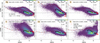 |
Fig. 5 Observed [X/M] vs. [M/H] abundance ratios for the α-elements (O, Mg, Si, S, Ca, Ti) from MWM DR19 for the entire galactocentric region between 3 and 15 kpc compared with the best fit CE model results (dotted curves) for all species. The spacing between the dots represent the discrete evaluation points during the time of the GCE simulation. The color coding represents the number of stars on the observational chemical map of the MW, and grey squares represent bins containing a single star. The red and black filled circles mark the path of the high-Mg and low-Mg stellar sequences, respectively, while the gray dots correspond to the so-called merger phase. This color coding is the same as in Fig. 12 and the top panel of Fig. 6. In each panel, the metallicity and [X/M] abundance ratio are displayed at the exact time of the Sun’s birth during the simulation, which is also marked with a star symbol. The multiplication factor applied for the stellar nucleosynthetic yields of the relevant element is also indicated in the upper right corner of the plots. |
Results for the global and regional fits.
4.2 Fitting the data with lmfit algorithm
To choose the best-fit model, we created a pipeline that starts with the separation of the observational data into the high- and low-Mg populations and finishes with reporting the optimized GCE model via the nested OMEGA+ code. The lmfit Python package contains the fitting method solving for least squares with the Levenberg-Marquardt (LM) algorithm. This package provides tools to build complex fitting models for non-linear least-squares problems and to apply these models to the measured data. The χ2-statistic is defined as:
![$\[\chi^2=\sum_i^N \frac{\left[y_i^{\text {meas }}-y_i^{\text {model }}(\mathbf{p})\right]^2}{\epsilon_i^2},\]$](/articles/aa/full_html/2025/07/aa53951-25/aa53951-25-eq29.png) (14)
(14)
where N is the number of values at which the function is evaluated, ![$\[y_{i}^{\text {meas}}\]$](/articles/aa/full_html/2025/07/aa53951-25/aa53951-25-eq30.png) is the set of measured data,
is the set of measured data, ![$\[y_{i}^{\text {model}}(\mathbf{p})\]$](/articles/aa/full_html/2025/07/aa53951-25/aa53951-25-eq31.png) is the model, p is the set of variables in the model to be optimized in the fit, and εi is the estimated uncertainty in the data. This method is based on an objective function that takes a set of variables, then calculates the model and returns a residual array of
is the model, p is the set of variables in the model to be optimized in the fit, and εi is the estimated uncertainty in the data. This method is based on an objective function that takes a set of variables, then calculates the model and returns a residual array of ![$\[y_{i}^{\text {meas}}-y_{i}^{\text {model}}(\mathbf{p})\]$](/articles/aa/full_html/2025/07/aa53951-25/aa53951-25-eq32.png) . To perform the parameter optimization, a minimization is carried out on the residuals with scipy.optimize6. After a fit has been completed successfully, the estimated uncertainties for the fitted variables and correlations between pairs of fitted variables are calculated by inverting the Hessian matrix, which represents the second derivative of fit quality for each variable parameter.
. To perform the parameter optimization, a minimization is carried out on the residuals with scipy.optimize6. After a fit has been completed successfully, the estimated uncertainties for the fitted variables and correlations between pairs of fitted variables are calculated by inverting the Hessian matrix, which represents the second derivative of fit quality for each variable parameter.
The method of dividing the locus of high- and low-Mg populations from the observed abundances is explained in Sect. 2.3. In each iteration phase, the observed median high-Mg and low-Mg sequences are interpolated over the output [M/H] values. This intrinsically gives higher weights to the data points that belong to the thin disk, as the metallicity steps during the GCE simulation get smaller when more stars are created within a time step. The [M/H] versus [Mg/M] parameter spaces then correspond to the following arrays,
![$\[\begin{aligned}& \mathbf{w}_{\text {global }}=\left\{w_{[\mathrm{M} / \mathrm{H}], \text { global }}, w_{[\mathrm{X} / \mathrm{M}], \text { global }}\right\}, \\& \mathbf{w}_n=\left\{w_{[\mathrm{M} / \mathrm{H}], n}, w_{[\mathrm{X} / \mathrm{M}], n}\right\},\end{aligned}\]$](/articles/aa/full_html/2025/07/aa53951-25/aa53951-25-eq33.png)
featuring the global and the regional data (describing the nth region, where n ∈ {1; 2; ...; 6}), respectively. The w[X/M],global and w[X/M],n notations provide the ymeas values within Eq. (14). Within our analysis, the data-model residual returned by the objective function is the difference between the observational data and the model, where the latter is based on the output of the GCE code. The results of an OMEGA+ run contain all the relevant quantities to analyze the GCE model (e.g., Galactic gas mass, SNe type Ia and II rate, elemental abundances).
The global and regional parameters that are varied are
![$\[\begin{aligned}& \mathbf{P}_{\text {global }}=\left\{t_{\max }, \tau_1, \tau_2, \tau_{\text {up }}, \sigma_2 / \sigma_1, \sigma_{\text {tot }}, f_{\mathrm{Mg}}\right\}, \\& \mathbf{P}_{\text {regional }}=\left\{t_{\max }, \tau_1, \tau_2, \tau_{\text {up }}, \sigma_2 / \sigma_1\right\},\end{aligned}\]$](/articles/aa/full_html/2025/07/aa53951-25/aa53951-25-eq34.png)
where each parameter spreads within a range detailed in Table 1. These vectors are considered the set of variables p in Eq. (14).
This study is computationally built upon three main sequential blocks. Initially, we performed a global fit on the galactic sample by optimizing the Pglobal parameters to fit the [Mg/M]–[M/H] parameter plane. We used Mg as the key tracer as it is one of the most accurately measured and precisely derived elements published in MWM and its zero-point offset is negligible for RGB stars. The estimated MWM precision varies between 0.04 and 0.05 dex (M25). Then, in the second phase, the optimal global data set is fixed, but we allow the yield multiplication factors, fX, to vary for the other chemical species to match the [X/M] observations. Finally, the regional fits are optimized by fixing the global parameter σtot as well as fX while fitting the Pregional variables.
We note that the distributions of the components of the residual array are approximated as Gaussians, because investigating the correlations and degeneracies between the GCE parameters would lead us beyond the scope of this study. The errors of the Pglobal and Pregional parameters are reported by the LM-algorithm. However, the uncertainties of the resulting present values of the inflow rate, SFR, SNe rates, and the gas and stellar mass of the Galaxy must be estimated with a different approach, as they are not free parameters. Therefore, we implemented a boot-strap analysis, which involves 10 000 random resamplings of the observational data, and the distributions of the obtained values are approximated with Gaussians. Finally, the 1σ standard variations provide estimates of the uncertainties.
The best-fit GCE model parameters with confidence levels are reported in Table 3 both for the global and regional cases. The yield multiplication factors and the discrepancies of Δ[M/H] and Δ[X/M] from the solar zero-point at the time of the birth of the Sun are summarized later in Table 4. The solar reference abundance scale used in MWM is Grevesse et al. (2007); therefore, we implemented the same table in the GCE model to normalize the chemical abundances.
Applied fX global yield multiplication factors and their discrepancies.
5 Results and discussion
The model GCE predictions are obtained by fitting the abundance ratio [Mg/M] and [M/H] of stars in the MWM DR19 data set using the lmfit technique. The global fits are discussed in Sect. 5.1. In Sect. 5.2, we interpret our results in terms of the inside-out formation scenario. In Sect. 5.5, we compare our findings with the predictions of S21.
The first panel of Fig. 5 shows the observed [Mg/M] versus [M/H] abundance ratios derived in MWM DR19 within the disk between 3 and 15 kpc compared with the best-fit GCE model results (dotted curves). We note that this parameter plane was used for obtaining the best-fit global GCE model. Figures 6 depicts the inflow and outflow rate, SFR, SNe rates, and the evolution of gas and stellar mass according to the global model, while Fig. 7 is linked to the regional results. The characteristic ascending and descending accretion timescales and the galactic times of the second infall are plotted in Fig. 8, the ratios and the sums of the surface mass densities are represented in Fig. 9. The evolution of the individual α-elements, odd-Z elements, and metallicity are tracked in Figs. 5 and 12, and 10–11, respectively.
5.1 Global evolution of the Galactic disk
The evolution of the global observables (inflow and outflow, SFR, SNe rate, galactic and stellar mass) is given in Fig. 6. The final quantities obtained at the end of the simulations are called present-day values, and their final values are compared to the literature values derived mostly based on solar neighborhood observations and listed in Table 2.
The inflow and the delayed outflow trends are plotted in the top panel of Fig. 6. The maximum inflow rate during the formation phase, which happened in the first 2 Gyr, is 28.72 M⊙ yr−1 at 0.15 Gyr, while the maximum outflow rate during this period is 8.58 M⊙ yr−1 at 0.35 Gyr. This high-Mg phase is followed by the ascending (accretion) branch of the merger event, in which the inflow rate sharply increases with time after a short gap. In the gap, the inflow and outflow rates reached their minimum at around 1.45 Gyr and 2.05 Gyr, respectively. During the episode of the second infall, the inflow rate peaked at 4.13 Gyr with a value of 20.15 M⊙ yr−1, and the outflow rate followed this behavior at 4.75 Gyr with a maximum of 6.80 M⊙ yr−1. The outflow rate follows the inflow function, and the time of the second peak is delayed by 0.6 Gyr.
In the last 1–2 Gyr, the rates of the outgoing and the incoming matter declined, approaching zero, while a weak net inflow is still observed, which is also consistent with findings in the literature. The current galactic inflow rate was investigated by, for instance, Marasco et al. (2012) and Lehner & Howk (2011), and found to be (1.1 ± 0.5) M⊙ yr−1. This result is consistent with our study, since we have obtained a value of 1.4 M⊙ yr−1. We find that the present-time global outflow rate is lower than the inflow rate, 1.21 M⊙ yr−1. In accordance with our model, Fox et al. (2019) derived empirical constraints on the flow rates via the UV absorption-line high-velocity clouds. Their results of (0.53 ± 0.31) M⊙ yr−1 and (0.16 ± 0.10) M⊙ yr−1 describing the lower limits of inflow and outflow, respectively, also suggest that the MW is currently in an inflow-dominated state. Substantial mass flux in both directions supports a galactic fountain model, in which gas is constantly recycled between the disk and the halo (Fox et al. 2019).
The global SFR throughout the simulation time is presented in the second panel of Fig. 6. A pattern similar to the inflow rate can be seen with a delay, as prescribed by Eq. (4). Consequently, the SFR also shows two peaks occurring after the times of the first (SFRmax,1 = 7.15 M⊙ yr−1) and second infall (SFRmax,2 = 7.42 M⊙ yr−1) events, separated by a gap reaching its minimum at 2.25 Gyr. The second peak in the SFR occurs 4.90 Gyr after the first one. Compared to the second peak of the inflow rate, the SFR shows a delay of 0.3 Gyr. A present-day value of 1.26 M⊙ yr−1 is predicted at the end of the simulation, which lies within the observed range of 1.54 ± 0.56 M⊙ yr−1, determined from young stellar objects detected by Spitzer (Robitaille & Whitney 2010).
The occurrence rates of SNe types Ia and II during the simulation are depicted in the third panel of Fig. 6. Type II SNe follow the trend exhibited by the inflow-driven SFR, while SNe Ia have a characteristic delay. Both curves have the two-peak shape. The explosion rates of SNe types II and Ia reaches a minimum within the gap at Galactic ages of 2.15 Gyr and 3.05 Gyr, respectively. The first and second bursts of the rate of SNe type II are separated by 4.4 Gyr (exactly as the SFR), while the rate of SNe type Ia experienced a broader gap of about 5.9 Gyr. In the Galactic disk, the final values reached in our model are 0.858 · 10−2 yr−1 for SNe II and 4.313 · 10−3 yr−1 for SNe Ia, where we applied Prantzos et al. (2011) as an observational benchmark for the simulations (see Table 2). The number of SNe type II tends to be underestimated, though this issue was also noticed by S21. We note that varying the slope of the IMF cannot solve this under-estimation. If we increase the upper mass limit for SNe type II, the abundance of the α-elements and the SNe II rate is not significantly higher. Possible extra sources, like magneto-rotational SNe, may be implemented, that would lead us beyond the scope of this paper.
The evolution of the mass of the gas, Mgas, displays two peaks with a gap at ~2 Gyr. The strictly increasing function is derived by the sum of the differences between the mass locked in stars and the stellar ejecta (mass loss). These masses are plotted as functions of the Galactic age in the bottom panel of Fig. 6. The final mass of the gas reached is (0.84 ± 0.17) × 1010 M⊙ which is consistent with the observation of (0.81 ± 0.45) × 1010 M⊙ (Kubryk et al. 2015). We also have good agreement with the present-day value of the total stellar mass as we obtained (3.4 ± 0.1) × 1010 M⊙, near the reference value of (3.5 ± 0.5) × 1010 M⊙ found by (Flynn et al. 2006).
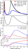 |
Fig. 6 Inflow and outflow rates (top panel), SFR (second panel), rates of SNe type Ia and II (third panel), Galactic mass, M⋆, enclosed in stars, and mass, Mgas, of the gas (bottom panel) as a function of galactic age, where t = 0 Gyr is the beginning of the Galactic formation and t = 14 Gyr is the present. The shaded areas with the corresponding colors represent the present-day measured values for each parameter (see Table 2). The inflow rate presented in the top panel includes the highMg (formation) and low-Mg (merger relaxation) phases, that are marked with red and black curves, while the rising accretion of the merger phase is marked with gray. |
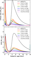 |
Fig. 7 Top: inflow rates as a function of galactic age, where t = 0 Gyr is the beginning of the Galactic formation, and t = 14 Gyr is present. Bottom: SFR as a function of time. The dashed and colored curves show the results of the global and the regional best-fit simulations, respectively. |
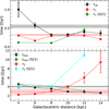 |
Fig. 8 Characteristic ascending and descending accretion timescales (τ1, τ2, and τup) and time delay (tmax) from the best-fit results as a function of Galactocentric distance R [kpc]. While the continuous lines represent the regional fits, the global value is indicated by dashed lines. Error bars and shaded areas show the estimated uncertainties of the fitted global and regional parameters. Results from S21 are denoted with green and cyan. |
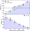 |
Fig. 9 Ratio (top panel) and the sum of the surface mass densities (bottom panel) related to the second and first infall events as a function of Galactocentric distance R [kpc]. The dashed line in the top panel represents the global fitted value, and the shaded area is the related uncertainty. Note: the errors associated with the total regional surface mass densities are calculated as described in the text. Results from S21 are denoted in green. |
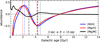 |
Fig. 10 Evolution of the [M/H], [Mg/H], and [Mg/M] abundance ratios as a function of Galactic age [Gyr] are marked with blue, red, and black colors, respectively. Note: a conversion relation of [Mg/H] = [Mg/M] + [M/H] holds for the values. The curves represent the result of the best-fit global model. Vertical dotted and dashed lines respectively represent the maxima and minima of each abundance curve within the range of 1–7 Gyr, where t = 0 Gyr is the beginning of the Galactic formation, and t = 14 Gyr is present. |
5.2 Evolution of the disk along the Galactocentric radius
In this section, we evaluate the regional results, and assess the consistency with the global GCE model of the MW. The regional and global best-fit model results are summarized in Table 3. The inner zone was fitted based on a total of 69 057 stars, the middle zone contains the highest number of 271188 stars, that encompasses the solar neighborhood, while only 53798 stars are contained in the outer regions.
Within the six modeled regions in the top panel of Fig. 7, the time of the second infall event ranges between tmax = 2.24 Gyr and 4.66 Gyr. It happened earlier in the outermost regions, and as time elapsed it successively reached the regions closer to the Galactic center (see also Table 3 and the bottom panel of Fig. 8). This suggests that the gravitational interaction between the potentially accreted dwarf galaxy and the early MW started about 11.3 Gyr ago, at the distance of R6 = 14 kpc and finished about 2 Gyr later, 9.5 Gyr ago at R1 = 4 kpc. The global model also suggested that it happened around the Galactic age of 4.13 Gyr (i.e., 10 Gyr ago) on average. We constructed the sum of the masses accreted in each region consistently with the best-fit global model. As a result of this consistent coupling between the regional and global models, the global present-day inflow rate shows a good agreement with the sum of the regional values.
In each region, there is a pause in the inflow rate between the first and second infall events at the Galactic ages of 1.25–1.85 Gyr. The regional inflow curves in the top panel of Fig. 7 show that the lowest inflow rate was usually experienced earlier in regions farther from the Galactic center. It could be also explained by a merger event affecting the outer Galaxy first. Moreover, the maximum values of the inflow rates associated with each infall event have a significant difference within the inner zone. In contrast, in the middle and outer zones, the peaking values are generally similar. The maximum inflow rate during the merger typically ranges between 0.70 M⊙ yr−1 and 5.97 M⊙ yr−1. The highest value corresponds to the second region centered at 6 kpc, then decreases toward the outer regions along with the shifting to earlier Galactic ages. We find that the difference between the first and second maximum values of the inflow rate is lower as the distance from the center increases. In addition to the inflow, the regional fits show that the present-day inflow rate is 0.08 M⊙ yr−1 in the innermost region, whereas it exhibits an increasing trend and reaches a final value of 0.21 M⊙ yr−1 in the outermost region. The sum of the six present-day values is 0.895 M⊙ yr−1, which is consistent with that of obtained by the global fit, 0.737 M⊙ yr−1 as well as with the references in Table 2.
The bottom panel of Fig. 7 shows that the SFR follows a delayed trend compared to the inflow rate. It also peaks at different times as the Galactocentric distance varies. The first peak in the SFR is associated with the rapid formation phase, around 0.25 Gyr in the six annular regions and globally. This suggests a ≈100-Myr-long delay from the inflow during the formation of the Milky Way. The further the region, the earlier the second SFR burst (probably triggered by the merger) is. The second SFR burst peaks at 4.25 Gyr in the sixth region and 5.25 Gyr in the first region. Compared to the time of the second infall event, the locus of the second starburst has a more significant delay than the first infall. It consistently becomes longer as the distance from the center increases, as the inner, middle, and outer zones experienced the delay between the infall and the SFR around 0.8 Gyr, 1.1 Gyr, and 1.5 Gyr.
The time gap separating the two starbursts also shows a trend as it is shorter with increasing the distance, and the local minima of the six regional SFR functions shift to earlier ages. In addition, the maximum SFR after the second infall mostly decreases with the distance except for the second region. The results for the final SFR show a weak, decreasing trend from the value of 0.19 M⊙ yr−1 in the first region to 0.12 M⊙ yr−1 in the sixth region. These values are consistent with the global result, as the sum of each present-day rate is 1.01 M⊙ yr−1 while the global fitted value is 1.11 M⊙ yr−1. Our results are in agreement with the reference of 1.54 ± 0.56 M⊙ yr−1 (Robitaille & Whitney 2010).
In Fig. 8, we plot the characteristic ascending and descending accretion timescales and time delay from the best-fit results. The τ1 parameter that drives the short relaxing time of the intense first infall does not show a significant trend with the Galactocentric radius, as it is roughly constant between 0.16–0.32 Gyr, with a global value of 0.322 Gyr. The τ2 descending branch of the second infall lasts longer when moving to the outer regions. The furthest zone shows a significantly longer relaxing time of 6.0–9.4 Gyr following the second infall event, compared to the closer zones where it ranges between 2.10–4.3 Gyr. This suggests that the relaxation episode following the merger event was weaker and slower in the more distant regions. The global value derived for τ2 is 2.86 Gyr, representing an average along the disk.
According to our six regional models, the τup, that represents the intensity of the exponentially ascending branch of the second infall event, varies between 0.29 and 1.23 Gyr throughout the regions, and is 0.55 Gyr for the best-fit global model, consistent with the regional results. This ascending phase of the accretion lasts the longest within the first region and declines until the third region centered at 8 kpc. It does not show any significant variation or trend in the outer zone. This generally suggests a more moderate accretion in the middle and outer zone compared to the inner one.
The surface mass density of the infalling matter captured during the entire Galactic evolution is σtot = 161.5 M⊙pc−2, which was distributed onto the six regions as discussed in Sect. 3.2, and listed in Table 3. The regions show an exponentially declining trend of surface mass density as a function of distance. However, the σ2/σ1 ratio is 7.614 in the global model, while it spans an interval of [1.934; 14.893] in the six separated regional models. This means that the density ratio increases toward the outer regions, whereas it has a value higher than one in each region. In other words, in the very first region, the second infall event provided a gas surface density two times larger than the first infall, then moving to the last region, this ratio grows until over 14 (see Fig. 9).
These values show that although the total mass of the infalling matter decreases toward the outermost region (86.7 M⊙ yr−1 in the inner zone, 51.0 M⊙ yr−1 in the middle zone, and 23.7 M⊙ yr−1 in the outer zone), the mass proportion originating from the second infall gets more significant. Therefore, by moving toward the outer regions their mass are more and more dominantly increased by the merger event. The results obtained here are consistent with those of S21, where the GCE models having a resolution of three regions suggest the following. The inner galactocentric zone enclosed between 2 and 6 kpc received surface densities with a ratio of ![$\[3.805_{-0.113}^{+0.078}\]$](/articles/aa/full_html/2025/07/aa53951-25/aa53951-25-eq35.png) , the middle zone between 6 and 10 kpc is best fit with a ratio of
, the middle zone between 6 and 10 kpc is best fit with a ratio of ![$\[5.635_{-0.162}^{+0.214}\]$](/articles/aa/full_html/2025/07/aa53951-25/aa53951-25-eq36.png) , and the outer one defined from 10 to 14 kpc is best fit with a ratio of
, and the outer one defined from 10 to 14 kpc is best fit with a ratio of ![$\[10.348_{-0.171}^{+0.188}\]$](/articles/aa/full_html/2025/07/aa53951-25/aa53951-25-eq37.png) .
.
The fact that the inner Galactic regions have shorter infall timescales in the high-Mg phase suggests a faster formation and assembly compared to the outer regions, supporting the inside-out formation scenario. As demonstrated by the observational data in Fig. 3, the locus of the low-Mg sequence is shifted toward lower metallicities as the distance increases from the Galactic center. These outer regions may experience a weaker and less efficient chemical enrichment as a result of longer accretion timescales. Therefore, a generally lower metallicity and Mg-abundance was reached at the end of the model (Fig. 11). In addition, the high-Mg phase has fewer stars as a function of Galactocentric distance, and we associate the more prominent low-Mg group with a larger surface density ratio there. A similar trend of growing σ2/σ1 ratio was found by Palla et al. (2020).
5.3 Evolution of metallicity and magnesium
Figures 10 and 11 show the global and regional evolution of the [M/H], [Mg/H], and [Mg/M] abundance ratios in the stars as a function of Galactic age, where vertical lines mark the times of the local maximum and minimum points from the simulation. The [Mg/H] and metallicity display similar evolutionary tracks as a function of time, while the [Mg/M] shows an inverse trend. The [M/H] versus [Mg/M] are plotted in the first panel of Fig. 5.
As we can infer from Fig. 10 (black model curve), the [Mg/M] abundance reaches its highest value shortly after the formation period, and when SNe Ia start to contribute, [Mg/M] generally declines between 1–3 Gyr, while both metallicity (blue curve) and [Mg/H] (red curve) are sharply rising until t ≈ 2 Gyr. According to our best-fit model covering the entire disk, magnesium and metals decline relative to hydrogen after t ≈ 2 Gyr, when the second infall event begins.
Subsequently, this merger event causes an enrichment of Mg relative to metallicity at around 4 Gyrs (see the rising phase of the loop in the first panel of Fig. 5). During this period, it significantly increases the rate of SNe II, while the SNe Ia reach their maximum with a delay of ~2 Gyr (see the third panel of Fig. 6). The growing number of exploding white dwarfs again causes a moderately steep decline of [Mg/M]. Shortly after the peak of the second infall at tmax, there is a minimum of Mg and metallicity relative to H, while the [Mg/M] had a temporary maximum. Afterward, the [Mg/H] and metallicity steadily increase, while [Mg/M] mildly decreases for about 9 Gyr to the present time. Throughout the entire simulation, [M/H] and [Mg/H] show similar trends, in a way that the overall metallicity [M/H] is delayed by < 0.5 Gyr from [Mg/H].
The abundance ratios of [M/H], [Mg/H], and [Mg/M] in the six regions are depicted in Fig. 11. When comparing their evolution curves, we see that the minimum [Mg/M] reached after the formation phase tends to be consistently larger at regions at greater Galactocentric distance, and occur progressively earlier in the model (at time from 2.4 to 3.2 Gyr). Then at around 2.7–4.5 Gyr, due to the burst in SNe type II induced by the merger event, [Mg/M] experiences a local maximum, and monotonously declines until the present day as SNe Ia occur at a longer and delayed timescale. The maximum [Mg/M] is reached at ~6 Gyr in the R1 innermost region and ~3.1 Gyr in the R6 outermost region.
The [M/H] and [Mg/M] reach a temporary maximum between the first infall event’s relaxation phase and the second infall’s ascending branch. These maxima happened the earliest at a Galactocentric distance of 14 kpc (~1.5 Gyr) and later at ~2.2 Gyr within the region centered at 4 kpc. The second peak of the infall rate causes a sudden drop in both abundances, which is seen as a loop in, for example, Fig. 5. These minimum values become larger within the inner zone, while the Galactic age is almost 5 Gyr in the first region and ~3 Gyr in the sixth one. The present-day abundance values can also be observed in the regional panels of Fig. 11 as the final values of the evolutionary curves. Our model predictions are consistent with the observations, which predict a declining present-day radial abundance gradient of [Mg/H] and [M/H]. These trends in the regional results support the presence of a major merger event in Galactic history that first started to interact with the outer MW and then gradually approached the inner Galaxy.
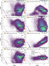 |
Fig. 12 Same as Fig. 5 for the light odd-Z (Na, Al, K), iron-peak odd-Z (V, Mn, Co), and iron-peak even-Z (Cr, Ni) elemental abundances. Note: ⊗ drives caution to V because of the high observational uncertainty. |
5.4 Evolution of the individual elements
5.4.1 Evolution versus metallicity
The best-fit evolutionary curves for the elements are shown in Figs. 5 and 12, compared to the SDSS-V MWM DR19 observations. The reversed feature in the [M/H] evolution generally appears around the Galactic age of 4 Gyr when the intense accretion of primordial-composition gas occurs, diluting the ISM and thereby reducing the overall metallicity. The evolution of each α-element as a function of metallicity is depicted in Fig. 5 for the entire disk. The observed chemical evolution patterns of Mg, Si, S, and Ca are reproduced. On the other hand, for O and Ti GCE predictions also tend to disagree during the merger event and the low-Mg phase, independently from any correction factor applied to the theoretical stellar yields. The observed abundances of these latter elements are derived with a typical uncertainty of 0.056 dex and 0.082 dex in the solar neighborhood sample, respectively (M25). Oxygen is determined with an excellent quality, involving a slight zero-point offset, no significant dependency on effective temperature, high precision (M25); thus, it can be used safely throughout a large enough parameter space covered by our study (as in the target selection described in Sect. 2.2). The model behavior at the low metallicity of [M/H] ≈ −2 dex exhibits an under estimation of abundances of S and Ca, while an over estimation of Ti compared to the observation.
The thin and thick disks are sharply separated on the chemical map drawn by the observations of O as well. However, it has been noted before that there are difficulties in deriving [O/M] from the atomic absorption lines in optical wavelength ranges (e.g., GALAH, De Silva et al. 2015) and from the molecular lines in near-infrared spectra of stellar atmospheres (APOGEE). As studied on golden cross-matched samples and also outlined by Hegedűs et al. (2023), the discrepancies between the [O/H] abundances derived by sky survey programs range from 0.03 to 0.20 dex for giant stars. Therefore, we can observe some disagreement in the slopes displayed by APOGEE and GALAH data of the [M/H] versus [Mg/O] high-α and low-α sequences (see, e.g., Weinberg et al. 2019; Griffith et al. 2019). Moreover, the median Δ[O/H] abundance difference between MWM DR19 and GALAH DR3 is −0.05 dex with a significant scatter of 0.22 dex (M25). In contrast, titanium is the least precise α-element published in MWM DR19 and was derived with fair precision and accuracy due to the fact that Ti – with its relatively weak absorption lines – was possible to be measured reliably only in a narrow parameter region, between 4000 K ≤ Teff ≤ 5500 K and around solar metallicity for giants. While the median Δ[Ti/H] = −0.05 ± 0.28 dex difference and scatter as compared to GALAH DR3 is similar to the case of O, the significant temperature dependence of [Ti/H] detection in the solar neighborhood may be complex. The discrepancies might be due to the difficulty of fitting the mostly blended Ti lines or NLTE effects (M25).
The evolution of the light odd atomic number and iron-peak elements (Na, Al, K, V, Cr, Mn, Co, and Ni) is depicted in Fig. 12. The abundances of Cr, Mn, and Ni are well tracked throughout the chemical maps, whereas the distribution patterns of Na, Al, K, and Co are only fairly reproduced. In most cases, especially of K, Cr, and Ni, we still observe a discrepancy at low metallicity, whereas obtaining a good agreement near the solar value at the same time. Generally, we modeled the iron-peak elements more accurately than the light odd-Z elements. Among the iron-peak elements, the MWM Ni abundances have excellent quality, and can be used reliably above 4250 K, according to the estimated overall precision. Moreover, there is a very good agreement with GALAH DR3 (M25). On the contrary, V abundances are categorized as of poor quality, and it is advised to use [V/H] values with caution (M25). The comparison detailed in M25 with GALAH DR3 data showed a strong correlation with Teff and a mean discrepancy of −0.13 ± 0.43 dex. The other elements in Fig. 12 are either determined with a good or fair accuracy and precision in MWM. The reliable parameter ranges for these elements are typically restricted (M25). The reason for the discrepancies between the model and the MWM data may be a result of both observational uncertainties (e.g., degeneracies between age and [M/H] (Jofré et al. 2019), LTE approximations, abundance derivation systematics) and model uncertainties (e.g., reaction rate uncertainties, space progenitor grids, and GCE model assumptions).
5.4.2 Evolution versus magnesium
Figure 13 shows the [X/Mg] abundances as a function of [Mg/H]. For the elements produced predominantly by CCSNe, the observations are expected to exhibit a uniform horizontal trend in the [X/Mg]–[Mg/H] parameter plane. For instance, in the first panel of Fig. 13, the O abundances from the MWM data show this trend with a relatively small scatter. The evolutionary curve has an ≈0.1 dex discrepancy, which is the result of not being able to fit both Mg and O accurately (see the first row of Fig. 5).
Generally O and Al are produced by CCSNe like Mg, thereby exhibiting a horizontal evolution along with the [Mg/H] abundance. The observation and theory normally agree, except, the distribution of the measured Na abundances, which steadily increases with [Mg/H]. We also see that the model for Al and K shows a slight [Mg/H] dependency not seen in the data. Na has only two, reasonably weak lines in the H-band and might be also affected by minor errors introduced by the telluric correction. For Al, a possible difficulty could be NLTE effects, which were not taken into account in the spectral grid in DR19 (M25). Si and K, which are dominantly produced by CCSNe, show divergent results. Silicon has a good agreement, while the model for [K/Mg] shows disagreements at [Mg/H] ≲ 0 and an offset from the observation. The S and Ca are produced in both CCSNe and SNe type Ia. Our GCE model for S reflects a minor discrepancy. Our model and the Ca measurements have a very good agreement.
Other elements such as Ti, V, Cr, Mn, Co, and Ni have contributions dominantly or closely exclusively from SNe Ia. Our model for Mn well fits the observational thin and thick disk sequences. Titanium and cobalt display a fair agreement with slight offsets of ~0.1 dex, while Cr fits only moderately the observations with a significant offset discrepancy. We would recommend to not use V abundances, since there is no recommended reliable parameter range in M25.
To summarize, the elements that are difficult to measure observationally, due to the lack of clearly detectable or well-defined spectral lines, have fair or poor quality values published in DR19. This is the case for Na, Ti, Co, and V (M25) and, thus, we were not yet able to derive strong conclusions from their comparison with GCE models. On the contrary, the observed abundances of O, Si, Ni, Al, S, K, Cr, and Mn are reported to have excellent or good reliability in general (M25). There still may be some unrevealed issues for Al, K, and Cr, though, such as the lack of NLTE corrections or unknown line blendings, as these elements exhibit discrepancies between the GCE model and MWM spectroscopy.
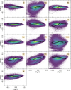 |
Fig. 13 Observed [X/Mg] vs. [Mg/H] abundance ratios for the α- and odd-Z elements from MWM DR19 throughout the entire galactocentric region between 3 and 15 kpc compared with the best-fit CE model results (dotted curves) for all species. The color coding represents the number of stars on the observational chemical map of the MW, and gray squares represent bins containing a single star. Note: ⊗ drives caution to V because of high observational uncertainty. |
5.4.3 Yield modifications
The fX yield multiplication factors are found during the global fit and then kept fixed when completing the regional fits (Table 4). As explained in Sect. 3.3, fX account for discrepancies between the observations and the theoretical yields. If the yields are correct and can reproduce the observed abundance trends, then the fX values should be close to one. However, we find that fX needs to be greater than one to fit the Mg, O, Na, Al, and Co abundances, while we applied fX less than one for Cr and Ni. The best fit yield correction factors show that the theoretical yield sets underlying our models systematically overproduce Cr and Ni and underproduce Mg, O, Na, Al, and Co. Such disparities between theoretical yields and observations exist for most yield sets (e.g., Griffith et al. 2021, for CCSN yields). If a different theoretical yield set is used, the factors found in this work will be varied, while the parameters describing the inflow function will practically provide an unaltered GCE picture of the MW. Most of the theoretical yield noise is captured by fX, without affecting the relevant results for our study, but as this factor is not metallicity dependent, it cannot fully correct for the yield errors.
We assume that stars formed at the same time as the Sun have the same solar chemical composition. This assumption is well established within the solar neighborhood, although it becomes an approximation when applied to the entire Galactic disk. To fulfill this assumption, the (1) definition of elemental abundance ratio [X/M] specifies that the individual values for the 14 chemical abundances have to be close to [M/H] = [X/M] = 0 for an SSP formed together with the Sun in time. We found a metallicity residual of Δ[M/H] = 0.020 dex, and between −0.066 and 0.069 dex for the Δ[X/M] individual abundances. (See Table 4 and Figs. 5 and 12.) Considering the typical uncertainties of the abundance determination from the stellar spectra (M25), these residuals are still in good agreement both with the observations and theoretical predictions. According to the precision classification terminology for DR19 abundances in M25 (detailed in their Table 5), Mg, O, Si, Ca, Mn, and Ni have an excellent precision of lower than 0.1 dex, while S, Al, K, and Cr have a good precision between 0.10 and 0.15 dexl while Ti, Na, V, and Co exhibit a fair or poor precision of above 0.3 dex. We note that the uncertainties provided here did not include accuracy and systematics. The abundance residuals are generally below or have the same order as the reported precision levels.
5.5 Comparison to Spitoni et al. (2021)
The simulations presented in this work are based on a revised two-infall scenario and support an inside-out formation as S21. Their comparison target selection ranged between the Galactocentric distances of 2 kpc and 14 kpc, separated into three regions. These regions contained 26 690 MW-disk stars from the APOGEE DR16 data set (Ahumada et al. 2020) and were used to fit the model. Here we use an expanded data set including 393 743 stars with a higher spatial resolution separated into six annular regions between 3–15 kpc. For comparison, the results for the inflow timescales, the time of the second infall, and the ratio of the surface mass densities obtained by S21 are listed in Table 3 (global model) and in Figs. 8 and 9 (regional models).
The inflow function directly before the second peak is constant at zero in S21, while our model applies a rising branch of accretion as well. Both models neglect the effect of radial stellar migration in the disk. Effective net gas outflows were not introduced by S21, whereas they invoked a previously enriched gas infall to correctly reproduce the [Mg/Fe] vs. [Fe/H] abundance ratio of the low-α sequence in the inner disk. Our GCE model involves a constant mass-loading parameter to drive the galactic winds permanently leaving the Galactic disk while allowing for an infall with primordial composition matter.
Both in the present work and in S21, Mg and Fe were used as key tracers, while the chemical maps of 14 elements beyond [Mg/Fe] vs. [Fe/H] were also reproduced here. As the source for the nucleosynthetic yields, S21 adopted the yield set of Woosley & Weaver (1995) for massive stars, and Iwamoto et al. (1999) for SNe type Ia. In their best-fit model, Mg and Si yields were artificially raised. In contrast, our study is based on the theoretical yields composed and published by the NuGrid collaboration and by FRUITY (Cristallo et al. 2016) for massive and AGB stars, respectively. The yields of SNe Ia come from the same reference work. We keep the yields of Fe untouched, also fFe = 1, as in S21, while the individual elemental contributions were modified according to Table 4.
As shown in Table 3 (for the global model) and Fig. 8 (for the regional models), the values and trends describing the time of the merger event and the accretion timescales generally agree well with S21. The agreement is also excellent in the region where the Sun is located (Fig. 8). The global and regional fit σ2/σ1 are listed in Table 3, and plotted in Fig. 9. Although the number of regions and the spatial boundaries of the separations in their study differ from those we used, an increasing trend was also observed with Galactocentric distance.
Minor differences between our results and S21 originate from using different observational data sets, not using the exact identical chemical model assumptions and computational techniques, and adopting different nucleosynthetic yield sets. In general, both results reflect a similar picture of Galactic history: our model and that of S21 share a similar growth of the Galactic disk following the inside-out scenario and predict analogous metallicity distribution functions. We also confirm the potential merger event at a Galactic age of around 4 Gyr, causing a well-defined gap in the SFR.
6 Conclusions
We studied the GCE of 14 elements based on a golden sample of 393 743 stars from the first data release (DR19) of the MWM spectroscopic sky survey part of SDSS-V. First, we analyzed the observed chemical map of our Galaxy. The separation between the chemical thin and thick disks was defined using [Mg/M] and in this work, we also discuss the high- and low-Mg sequences across the Galactocentric radii. The chemical maps of most elements considered here show similar trends to Mg, although sequences of odd-Z species such as Co, Mn, or V display different patterns as functions of metallicity. Following previous studies (e.g., Hayden et al. 2015), but with a larger sample of stars by an order of magnitude, we have found that the locus of the low-Mg sequence is gradually shifted toward lower metallicity in the outer regions, while the number of stars in the high-Mg population decreases both absolutely and relatively to the low-Mg group.
We present extended chemical evolution models for the Galactic disk and six galactocentric regions between 3 kpc and 15 kpc. The measured abundances of Mg constrained the model by utilizing the semi-analytical GCE code OMEGA+. We considered seven free global parameters related to the two infall episodes: the accretion relaxing timescales, τ1 and τ2, the characteristic duration of the merger phase, τup, the delay, tmax, and the ratio and sum of the surface mass densities associated with the second and first infall events, σ2/σ1 and σtot, and the Mg yield scaling factor, fMg. While performing the regional fits, the variables σtot and fMg were kept fixed. We drew the following conclusions describing the formation history based on our fittings of the observational chemical maps.
The OMEGA+ model obtained here suggests a general agreement with the recent MWM observations published in DR19 (M25). A significant delay time between the two gas infall episodes for the thick-disk and thin-disk formation is confirmed in all analyzed galactocentric regions. We find that the approximate value for the delay time ranges between 2.6 and 4.7 Gyr, confirming the results of S21, but on a much larger sample. Thus, we confirm the concept of a merger event approximately 10 Gyr ago over the course of Galactic history.
This prolonged merger event starts around 3 Gyr after the initial formation of the MW in the outer zone and 5 Gyr in the inner zone. As the Galactocentric radius is growing, a decrease in tmax produces a tighter loop starting at lower metallicities and allowing for only a higher value for the minimum of the Mg abundance during the infall event (Spitoni et al. 2019) When the Galaxy reaches the age of 8 Gyr, the rate of accreting matter dramatically falls (Fig. 7). Since our model represents a two-infall scenario, the first inflow event creates the high-α (or high-Mg) thick disk stars during Galactic formation; whereas the second allows for the birth of the low-α (or low-Mg) stars of the thin disk (Fig. 5).
-
The entire merger event lasts for about 5 Gyr and occurs earlier at larger Galactocentric distances. The ratios between the thin and thick disk surface mass densities grow toward the outer regions, in agreement that as we move toward external regions, the distribution of the MWM DR19 data sample represents fewer stars in the high-Mg phase compared to the low-Mg sequence. We derive an inside-out formation of the thin-disk of our Galaxy according to the best fit of our multi-zone CE simulation, meaning that the inner Galactic regions are assembled on a shorter timescale than the external parts.
The beginning of the merger may be estimated with the characteristic rising time of the accretion interval as tmax − τup; therefore, our results confirm the conclusions of Chaplin et al. (2020), as we find that the earliest time the merger could have begun was 11.5–11.9 Gyr ago in the outermost region.
Important observational constraints, such as the present-day inflow rate, SFR, SNe rates, and the stellar and gas mass, are reasonably well reproduced within the uncertainties. The six regional results are consistent with the global best-fit model for obtaining the present-day global inflow rate, SFR, and stellar and gas mass by the sum of the regional values.
The chemical evolution is substantially driven by the stellar yields. The solar composition is generally obtained within observational uncertainties (M25). The evolutionary curves show good agreement for the α-elements Mg, Si, and Ca, as well as for the odd-Z elements Na, Mn, Ni. Elements Al, K, Ti, and V, are not well reproduced. Discrepancies may originate from observational and model uncertainties, including unresolved or heavy blending in the spectra, The LTE approximations in the abundance determination, uncertainties in theoretical reaction rates, and assumptions about massive star black hole formation. Our implementation of yield correction factors allow for the relevant GCE results to be obtained relatively independently of the chosen yield set, with a ≲10% variation. Moreover, when performing the optimization based on Si instead of Mg, the GCE results suggest the same formation history with an inflow function characterized by a time of the second peak, inflow timescales, and the ratio and sum of the surface mass densities, which only changes by ≲15%.
We generally confirm the results obtained by S21, adopting similar GCE parametrization but using different stellar yields and a different set of observations to benchmark the GCE calculations. Our modeling study of the merger and dual-infall GCE for the disk also represents a scenario that is complementary to the one proposed by Sharma et al. (2021) and Prantzos et al. (2023), where the radial variation in the [α/M] versus [M/H] abundance parameter plane has been explained with stellar migration. In the future, the implementation of stellar migration, the variation of the SFR, along with the galactocentric distance, and the use of the subsequent most recent data sets from SDSS-V will serve as a further development for this framework.
Acknowledgements
VH and SzM acknowledge the support of Hungarian Academy of Sciences through MTA-ELTE Lendület “Momentum” Milky Way Research Group. Supported by the DKOP-23 Doctoral Excellence Program of the Ministry for Culture and Innovation from the Source of the National Research, Development and Innovation Fund and Lendület LP2023-10. BV, MP, and ML acknowledge the support of the Hungarian Academy of Sciences via the Lendület Program LP2023-10. This work was supported by the European Union’s Horizon 2020 research and innovation programme (ChETEC-INFRA – Project no. 101008324), and the IReNA network supported by US NSF AccelNet (Grant No. OISE-1927130). ML was also supported by the NKFIH excellence grant TKP2021-NKTA-64. E.J.G. is supported by an NSF Astronomy and Astrophysics Postdoctoral Fellowship under award AST-2202135. D.S. thank the National Council for Scientific and Technological Development – CNPq process No. 404056/2021-0. Funding for the Sloan Digital Sky Survey V has been provided by the Alfred P. Sloan Foundation, the Heising-Simons Foundation, the National Science Foundation, and the Participating Institutions. SDSS acknowledges support and resources from the Center for High-Performance Computing at the University of Utah. SDSS telescopes are located at Apache Point Observatory, funded by the Astrophysical Research Consortium and operated by New Mexico State University, and at Las Campanas Observatory, operated by the Carnegie Institution for Science. The SDSS website is www.sdss.org. SDSS is managed by the Astrophysical Research Consortium for the Participating Institutions of the SDSS Collaboration, including the Carnegie Institution for Science, Chilean National Time Allocation Committee (CNTAC) ratified researchers, Caltech, the Gotham Participation Group, Harvard University, Heidelberg University, The Flatiron Institute, The Johns Hopkins University, L’Ecole polytechnique fédérale de Lausanne (EPFL), Leibniz-Institut für Astrophysik Potsdam (AIP), Max-Planck-Institut für Astronomie (MPIA Heidelberg), Max-Planck-Institut für Extraterrestrische Physik (MPE), Nanjing University, National Astronomical Observatories of China (NAOC), New Mexico State University, The Ohio State University, Pennsylvania State University, Smithsonian Astrophysical Observatory, Space Telescope Science Institute (STScI), the Stellar Astrophysics Participation Group, Universidad Nacional Autónoma de México, University of Arizona, University of Colorado Boulder, University of Illinois at Urbana-Champaign, University of Toronto, University of Utah, University of Virginia, Yale University, and Yunnan University. For the lmfit Python package, Matthew Newville wrote the original version and maintains the project: https://lmfit.github.io/lmfit-py/index.html. This work made use of Astropy (http://www.astropy.org): a community-developed core Python package and an ecosystem of tools and resources for astronomy (Astropy Collaboration et al. 2013, 2018; Astropy Collaboration 2022). This research was supported by a grant from the European Astronomical Society thanks to the generous support of the MERAC Foundation and Springer Verlag.
References
- Abdurro’uf, Accetta, K., Aerts, C., et al. 2022, ApJS, 259, 35 [NASA ADS] [CrossRef] [Google Scholar]
- Ahumada, R., Allende Prieto, C., Almeida, A., et al. 2020, ApJS, 249, 3 [NASA ADS] [CrossRef] [Google Scholar]
- Allende Prieto, C., Beers, T. C., Wilhelm, R., et al. 2006, ApJ, 636, 804 [NASA ADS] [CrossRef] [Google Scholar]
- Astropy Collaboration, Robitaille, T. P., Tollerud, E. J., et al. 2013, A&A, 558, A33 [NASA ADS] [CrossRef] [EDP Sciences] [Google Scholar]
- Astropy Collaboration (Price-Whelan, A. M., et al.) 2018, AJ, 156, 123 [Google Scholar]
- Astropy Collaboration (Price-Whelan, A. M., et al.) 2022, ApJ, 935, 167 [NASA ADS] [CrossRef] [Google Scholar]
- Bergemann, M., Ruchti, G. R., Serenelli, A., et al. 2014, A&A, 565, A89 [NASA ADS] [CrossRef] [EDP Sciences] [Google Scholar]
- Boccioli, L., & Fragione, G. 2024, Phys. Rev. D, 110, 023007 [Google Scholar]
- Boissier, S., & Prantzos, N. 1999, MNRAS, 307, 857 [NASA ADS] [CrossRef] [Google Scholar]
- Boothroyd, A. I., & Sackmann, I. J. 2003, ApJ, 583, 1004 [NASA ADS] [CrossRef] [Google Scholar]
- Bowen, I. S., & Vaughan, Jr., A. H. 1973, Appl. Opt., 12, 1430 [NASA ADS] [CrossRef] [Google Scholar]
- Buck, T. 2020, MNRAS, 491, 5435 [NASA ADS] [CrossRef] [Google Scholar]
- Cescutti, G. 2008, A&A, 481, 691 [NASA ADS] [CrossRef] [EDP Sciences] [Google Scholar]
- Chiappini, C., Matteucci, F., & Gratton, R. 1997, ApJ, 477, 765 [Google Scholar]
- Chaplin, W. J., Serenelli, A. M., Miglio, A., et al. 2020, Nat. Astron., 4, 382 [Google Scholar]
- Chiosi, C. 1980, A&A, 83, 206 [NASA ADS] [Google Scholar]
- Cole, S., Lacey, C. G., Baugh, C. M., & Frenk, C. S. 2000, MNRAS, 319, 168 [Google Scholar]
- Côté, B., Ritter, C., O’Shea, B. W., et al. 2016, ApJ, 824, 82 [CrossRef] [Google Scholar]
- Côté, B., O’Shea, B. W., Ritter, C., Herwig, F., & Venn, K. A. 2017a, ApJ, 835, 128 [Google Scholar]
- Côté, B., Ritter, C., Herwig, F., et al. 2017b, in 14th International Symposium on Nuclei in the Cosmos (NIC2016), eds. S. Kubono, T. Kajino, S. Nishimura, T. Isobe, S. Nagataki, T. Shima, & Y. Takeda, 020203 [Google Scholar]
- Côté, B., Silvia, D. W., O’Shea, B. W., Smith, B., & Wise, J. H. 2018, ApJ, 859, 67 [CrossRef] [Google Scholar]
- Côté, B., Eichler, M., Arcones, A., et al. 2019, ApJ, 875, 106 [Google Scholar]
- Cristallo, S., Piersanti, L., Straniero, O., et al. 2011, ApJS, 197, 17 [NASA ADS] [CrossRef] [Google Scholar]
- Cristallo, S., Straniero, O., Piersanti, L., & Gobrecht, D. 2015, ApJS, 219, 40 [Google Scholar]
- Cristallo, S., Piersanti, L., & Straniero, O. 2016, in Journal of Physics Conference Series, 665, 012019 [Google Scholar]
- De Silva, G. M., Freeman, K. C., Bland-Hawthorn, J., et al. 2015, MNRAS, 449, 2604 [NASA ADS] [CrossRef] [Google Scholar]
- Ebinger, K., Curtis, S., Ghosh, S., et al. 2020, ApJ, 888, 91 [NASA ADS] [CrossRef] [Google Scholar]
- Flynn, C., Holmberg, J., Portinari, L., Fuchs, B., & Jahreiß, H. 2006, MNRAS, 372, 1149 [NASA ADS] [CrossRef] [Google Scholar]
- Fox, A. J., Richter, P., Ashley, T., et al. 2019, ApJ, 884, 53 [NASA ADS] [CrossRef] [Google Scholar]
- Francois, P. 1986, A&A, 160, 264 [NASA ADS] [Google Scholar]
- Fuhrmann, K. 1998, A&A, 338, 161 [NASA ADS] [Google Scholar]
- Gaia Collaboration (Katz, D., et al.) 2018, A&A, 616, A11 [NASA ADS] [CrossRef] [EDP Sciences] [Google Scholar]
- García Pérez, A. E., Allende Prieto, C., Holtzman, J. A., et al. 2016, AJ, 151, 144 [Google Scholar]
- Gilmore, G., & Reid, N. 1983, MNRAS, 202, 1025 [Google Scholar]
- GRAVITY Collaboration (Abuter, R., et al.) 2019, A&A, 625, L10 [NASA ADS] [CrossRef] [EDP Sciences] [Google Scholar]
- Greggio, L. 2005, A&A, 441, 1055 [NASA ADS] [CrossRef] [EDP Sciences] [Google Scholar]
- Grevesse, N., Asplund, M., & Sauval, A. J. 2007, Space Sci. Rev., 130, 105 [Google Scholar]
- Griffith, E., Johnson, J. A., & Weinberg, D. H. 2019, ApJ, 886, 84 [Google Scholar]
- Griffith, E., Weinberg, D. H., Johnson, J. A., et al. 2021, ApJ, 909, 77 [NASA ADS] [CrossRef] [Google Scholar]
- Grisoni, V., Spitoni, E., Matteucci, F., et al. 2017, MNRAS, 472, 3637 [Google Scholar]
- Gunn, J. E., Siegmund, W. A., Mannery, E. J., et al. 2006, AJ, 131, 2332 [NASA ADS] [CrossRef] [Google Scholar]
- Hayden, M. R., Bovy, J., Holtzman, J. A., et al. 2015, ApJ, 808, 132 [Google Scholar]
- Hegedűs, V., Mészáros, S., Jofré, P., et al. 2023, A&A, 670, A107 [NASA ADS] [CrossRef] [EDP Sciences] [Google Scholar]
- Heger, A., & Woosley, S. E. 2010, ApJ, 724, 341 [Google Scholar]
- Helmi, A., Babusiaux, C., Koppelman, H. H., et al. 2018, Nature, 563, 85 [Google Scholar]
- Iwamoto, K., Brachwitz, F., Nomoto, K., et al. 1999, ApJS, 125, 439 [NASA ADS] [CrossRef] [Google Scholar]
- Jofré, P., Heiter, U., & Soubiran, C. 2019, ARA&A, 57, 571 [Google Scholar]
- Kennicutt, Robert C., J. 1998, ApJ, 498, 541 [NASA ADS] [CrossRef] [Google Scholar]
- Khoperskov, S., Di Matteo, P., Haywood, M., Gómez, A., & Snaith, O. N. 2020, A&A, 638, A144 [NASA ADS] [CrossRef] [EDP Sciences] [Google Scholar]
- Kobayashi, C., Karakas, A. I., & Lugaro, M. 2020, ApJ, 900, 179 [Google Scholar]
- Kroupa, P. 2001, MNRAS, 322, 231 [NASA ADS] [CrossRef] [Google Scholar]
- Kubryk, M., Prantzos, N., & Athanassoula, E. 2015, A&A, 580, A126 [NASA ADS] [CrossRef] [EDP Sciences] [Google Scholar]
- Larson, R. B. 1976, MNRAS, 176, 31 [NASA ADS] [CrossRef] [Google Scholar]
- Larson, R. B. 1988, in NATO Advanced Study Institute (ASI) Series C, 232, Galactic and Extragalactic Star Formation, eds. R. E. Pudritz, & M. Fich, 459 [Google Scholar]
- Larson, R. 1992, in Star Formation in Stellar Systems, eds. G. Tenorio-Tagle, M. Prieto, & F. Sanchez, 125 [Google Scholar]
- Lehner, N., & Howk, J. C. 2011, Science, 334, 955 [NASA ADS] [CrossRef] [Google Scholar]
- Liang, J., Gjergo, E., & Fan, X. 2023, MNRAS, 522, 863 [Google Scholar]
- Majewski, S. R., Schiavon, R. P., Frinchaboy, P. M., et al. 2017, AJ, 154, 94 [NASA ADS] [CrossRef] [Google Scholar]
- Maoz, D., & Mannucci, F. 2012, PASA, 29, 447 [NASA ADS] [CrossRef] [Google Scholar]
- Marasco, A., Fraternali, F., & Binney, J. J. 2012, MNRAS, 419, 1107 [NASA ADS] [CrossRef] [Google Scholar]
- Matteucci, F. 2021, A&A Rev., 29, 5 [NASA ADS] [CrossRef] [Google Scholar]
- Matteucci, F., & Tornambe, A. 1985, A&A, 142, 13 [Google Scholar]
- Matteucci, F., & Greggio, L. 1986, A&A, 154, 279 [NASA ADS] [Google Scholar]
- McKee, C. F., Parravano, A., & Hollenbach, D. J. 2015, ApJ, 814, 13 [Google Scholar]
- McWilliam, A. 1997, ARA&A, 35, 503 [NASA ADS] [CrossRef] [Google Scholar]
- Pagel, B. E. J., & Tautvaisiene, G. 1995, MNRAS, 276, 505 [NASA ADS] [CrossRef] [Google Scholar]
- Pagel, B. E. J., & Tautvaisiene, G. 1997, MNRAS, 288, 108 [Google Scholar]
- Palla, M., Matteucci, F., Spitoni, E., Vincenzo, F., & Grisoni, V. 2020, MNRAS, 498, 1710 [Google Scholar]
- Pardi, M. C., Ferrini, F., & Matteucci, F. 1995, ApJ, 444, 207 [Google Scholar]
- Pejcha, O., & Thompson, T. A. 2015, ApJ, 801, 90 [NASA ADS] [CrossRef] [Google Scholar]
- Pignatari, M., Herwig, F., Hirschi, R., et al. 2016, ApJS, 225, 24 [NASA ADS] [CrossRef] [Google Scholar]
- Pignatari, M., Trueman, T. C. L., Womack, K. A., et al. 2023, MNRAS, 524, 6295 [Google Scholar]
- Prantzos, N. 2008, A&A, 489, 525 [NASA ADS] [CrossRef] [EDP Sciences] [Google Scholar]
- Prantzos, N., Boehm, C., Bykov, A. M., et al. 2011, Rev. Mod. Phys., 83, 1001 [NASA ADS] [CrossRef] [Google Scholar]
- Prantzos, N., Abia, C., Chen, T., et al. 2023, MNRAS, 523, 2126 [NASA ADS] [CrossRef] [Google Scholar]
- Pritchet, C. J., Howell, D. A., & Sullivan, M. 2008, ApJ, 683, L25 [NASA ADS] [CrossRef] [Google Scholar]
- Queiroz, A. B. A., Anders, F., Chiappini, C., et al. 2020, A&A, 638, A76 [NASA ADS] [CrossRef] [EDP Sciences] [Google Scholar]
- Ritter, C., Herwig, F., Jones, S., et al. 2018, MNRAS, 480, 538 [NASA ADS] [CrossRef] [Google Scholar]
- Robitaille, T. P., & Whitney, B. A. 2010, ApJ, 710, L11 [NASA ADS] [CrossRef] [Google Scholar]
- Roškar, R., Debattista, V. P., Quinn, T. R., Stinson, G. S., & Wadsley, J. 2008, ApJ, 684, L79 [Google Scholar]
- Schiavon, R. P., Phillips, S. G., Myers, N., et al. 2024, MNRAS, 528, 1393 [CrossRef] [Google Scholar]
- Schmidt, M. 1959, ApJ, 129, 243 [NASA ADS] [CrossRef] [Google Scholar]
- Searle, L., & Zinn, R. 1978, ApJ, 225, 357 [Google Scholar]
- Sharma, S., Hayden, M. R., & Bland-Hawthorn, J. 2021, MNRAS, 507, 5882 [NASA ADS] [CrossRef] [Google Scholar]
- Silva Aguirre, V., Bojsen-Hansen, M., Slumstrup, D., et al. 2018, MNRAS, 475, 5487 [NASA ADS] [Google Scholar]
- Smee, S. A., Gunn, J. E., Uomoto, A., et al. 2013, AJ, 146, 32 [Google Scholar]
- Souto, D., Cunha, K., Smith, V., et al. 2016, ApJ, 830, 35 [NASA ADS] [CrossRef] [Google Scholar]
- Souto, D., Cunha, K., Smith, V. V., et al. 2018, ApJ, 857, 14 [NASA ADS] [CrossRef] [Google Scholar]
- Spitoni, E., Romano, D., Matteucci, F., & Ciotti, L. 2015, ApJ, 802, 129 [NASA ADS] [CrossRef] [Google Scholar]
- Spitoni, E., Gioannini, L., & Matteucci, F. 2017a, A&A, 605, A38 [NASA ADS] [CrossRef] [EDP Sciences] [Google Scholar]
- Spitoni, E., Vincenzo, F., & Matteucci, F. 2017b, A&A, 599, A6 [NASA ADS] [CrossRef] [EDP Sciences] [Google Scholar]
- Spitoni, E., Silva Aguirre, V., Matteucci, F., Calura, F., & Grisoni, V. 2019, A&A, 623, A60 [NASA ADS] [CrossRef] [EDP Sciences] [Google Scholar]
- Spitoni, E., Verma, K., Silva Aguirre, V., et al. 2021, A&A, 647, A73 [EDP Sciences] [Google Scholar]
- Tinsley, B. M. 1980, Fund. Cosmic Phys., 5, 287 [Google Scholar]
- Ugliano, M., Janka, H.-T., Marek, A., & Arcones, A. 2012, ApJ, 757, 69 [NASA ADS] [CrossRef] [Google Scholar]
- Vincenzo, F., & Kobayashi, C. 2020, MNRAS, 496, 80 [NASA ADS] [CrossRef] [Google Scholar]
- Vincenzo, F., Spitoni, E., Calura, F., et al. 2019, MNRAS, 487, L47 [NASA ADS] [CrossRef] [Google Scholar]
- Weinberg, D. H., Holtzman, J. A., Hasselquist, S., et al. 2019, ApJ, 874, 102 [NASA ADS] [CrossRef] [Google Scholar]
- Wiersma, R. P. C., Schaye, J., Theuns, T., Dalla Vecchia, C., & Tornatore, L. 2009, MNRAS, 399, 574 [NASA ADS] [CrossRef] [Google Scholar]
- Wilson, J. C., Hearty, F. R., Skrutskie, M. F., et al. 2019, PASP, 131, 055001 [NASA ADS] [CrossRef] [Google Scholar]
- Woosley, S. E., & Weaver, T. A. 1995, ApJS, 101, 181 [Google Scholar]
OMEGA and OMEGA+ are part of the NuGrid chemical evolution package and are publicly available online at http://nugrid.github.io/NuPyCEE and https://github.com/becot85/JINAPyCEE
The MWM DR19 database can be downloaded from the SDSS-V Science Archive Server: data.sdss.org/sas/dr19/
All Tables
All Figures
|
Fig. 1 Observed stellar [α/M] vs. [M/H] abundance ratios from MWM DR19 (Meszaros et al., in prep.). The top panel shows a density plot for all the stars published, while the disk stars involved in the quality disk sample at the galactocentric regions 3 kpc ≤ R ≤ 15 kpc are depicted in the bottom panel. Color-coding of the bins starts from two, and gray squares represent bins containing a single star. The total number of stars is denoted by N. |
| In the text | |
|
Fig. 2 Chemical map of the Galaxy observed by MWM. The [X/M] vs. [M/H] relations are shown for the combined α-elemental ratio as well as the single elements from Mg to Ni for the global disk sample. Red and blue curves represent the median trends of the high- and low-Mg stars separated based on their Mg abundance. This separation and the metallicity boundaries of the thick and thin disk stars are indicated by the black solid and dashed lines in the panel of Mg. Note: ⊗ drives caution to V because of the high observational uncertainty. |
| In the text | |
|
Fig. 3 Observed stellar [Mg/M] vs. [M/H] abundance ratios from MWM DR19 (Meszaros et al., in prep.) for the six bins of different Galactocentric distances considered here. The regions plotted from the top are all 2-kpc-wide, and are centered at R1 = 4 kpc, R2 = 6 kpc, R3 = 8 kpc, R4 = 10 kpc, R5 = 12 kpc, and R6 = 14 kpc, respectively. The sample size in the i-th region is denoted by Ni. Red and blue squares represent the binned distributions of the high-Mg and low-Mg sequences, respectively. Details on the data selection are reported in the text. |
| In the text | |
|
Fig. 4 Version of the GCE results for [M/H] versus Mg and O abundance ratios obtained without applying yield correction factors. The other GCE parameters are fixed at the best-fit values found in Sect. 5. |
| In the text | |
|
Fig. 5 Observed [X/M] vs. [M/H] abundance ratios for the α-elements (O, Mg, Si, S, Ca, Ti) from MWM DR19 for the entire galactocentric region between 3 and 15 kpc compared with the best fit CE model results (dotted curves) for all species. The spacing between the dots represent the discrete evaluation points during the time of the GCE simulation. The color coding represents the number of stars on the observational chemical map of the MW, and grey squares represent bins containing a single star. The red and black filled circles mark the path of the high-Mg and low-Mg stellar sequences, respectively, while the gray dots correspond to the so-called merger phase. This color coding is the same as in Fig. 12 and the top panel of Fig. 6. In each panel, the metallicity and [X/M] abundance ratio are displayed at the exact time of the Sun’s birth during the simulation, which is also marked with a star symbol. The multiplication factor applied for the stellar nucleosynthetic yields of the relevant element is also indicated in the upper right corner of the plots. |
| In the text | |
|
Fig. 6 Inflow and outflow rates (top panel), SFR (second panel), rates of SNe type Ia and II (third panel), Galactic mass, M⋆, enclosed in stars, and mass, Mgas, of the gas (bottom panel) as a function of galactic age, where t = 0 Gyr is the beginning of the Galactic formation and t = 14 Gyr is the present. The shaded areas with the corresponding colors represent the present-day measured values for each parameter (see Table 2). The inflow rate presented in the top panel includes the highMg (formation) and low-Mg (merger relaxation) phases, that are marked with red and black curves, while the rising accretion of the merger phase is marked with gray. |
| In the text | |
|
Fig. 7 Top: inflow rates as a function of galactic age, where t = 0 Gyr is the beginning of the Galactic formation, and t = 14 Gyr is present. Bottom: SFR as a function of time. The dashed and colored curves show the results of the global and the regional best-fit simulations, respectively. |
| In the text | |
|
Fig. 8 Characteristic ascending and descending accretion timescales (τ1, τ2, and τup) and time delay (tmax) from the best-fit results as a function of Galactocentric distance R [kpc]. While the continuous lines represent the regional fits, the global value is indicated by dashed lines. Error bars and shaded areas show the estimated uncertainties of the fitted global and regional parameters. Results from S21 are denoted with green and cyan. |
| In the text | |
|
Fig. 9 Ratio (top panel) and the sum of the surface mass densities (bottom panel) related to the second and first infall events as a function of Galactocentric distance R [kpc]. The dashed line in the top panel represents the global fitted value, and the shaded area is the related uncertainty. Note: the errors associated with the total regional surface mass densities are calculated as described in the text. Results from S21 are denoted in green. |
| In the text | |
|
Fig. 10 Evolution of the [M/H], [Mg/H], and [Mg/M] abundance ratios as a function of Galactic age [Gyr] are marked with blue, red, and black colors, respectively. Note: a conversion relation of [Mg/H] = [Mg/M] + [M/H] holds for the values. The curves represent the result of the best-fit global model. Vertical dotted and dashed lines respectively represent the maxima and minima of each abundance curve within the range of 1–7 Gyr, where t = 0 Gyr is the beginning of the Galactic formation, and t = 14 Gyr is present. |
| In the text | |
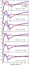 |
Fig. 11 Same as Fig. 10, but with the regional cases computed at R = {4, 6, 8, ..., 14} kpc. |
| In the text | |
|
Fig. 12 Same as Fig. 5 for the light odd-Z (Na, Al, K), iron-peak odd-Z (V, Mn, Co), and iron-peak even-Z (Cr, Ni) elemental abundances. Note: ⊗ drives caution to V because of the high observational uncertainty. |
| In the text | |
|
Fig. 13 Observed [X/Mg] vs. [Mg/H] abundance ratios for the α- and odd-Z elements from MWM DR19 throughout the entire galactocentric region between 3 and 15 kpc compared with the best-fit CE model results (dotted curves) for all species. The color coding represents the number of stars on the observational chemical map of the MW, and gray squares represent bins containing a single star. Note: ⊗ drives caution to V because of high observational uncertainty. |
| In the text | |
Current usage metrics show cumulative count of Article Views (full-text article views including HTML views, PDF and ePub downloads, according to the available data) and Abstracts Views on Vision4Press platform.
Data correspond to usage on the plateform after 2015. The current usage metrics is available 48-96 hours after online publication and is updated daily on week days.
Initial download of the metrics may take a while.