| Issue |
A&A
Volume 699, July 2025
|
|
|---|---|---|
| Article Number | A366 | |
| Number of page(s) | 21 | |
| Section | Catalogs and data | |
| DOI | https://doi.org/10.1051/0004-6361/202453179 | |
| Published online | 22 July 2025 | |
The EDGE-CALIFA Survey: An integral field unit-based integrated molecular gas database for galaxy evolution studies in the Local Universe
1
Argelander-Institut für Astronomie, University of Bonn,
Auf dem Hügel 71,
53121
Bonn,
Germany
2
Max-Planck-Institut für Radioastronomie,
Auf dem Hügel 69,
53121
Bonn,
Germany
3
Universidad Nacional Autónoma de México, Instituto de Astronomía,
AP 106,
Ensenada
22800,
BC,
Mexico
4
Instituto de Astrofísica de Canarias, Vía Láctea s/n,
38205,
La Laguna, Tenerife,
Spain
5
Department of Astronomy, University of Maryland,
College Park,
MD
20742,
USA
6
Department of Astronomy, University of Illinois,
Urbana,
IL
61801,
USA
7
Departamento de Astronomía, Universidad de Concepción, Barrio Universitario,
Concepción,
Chile
8
Department of Physics, University of Alberta,
4-181 CCIS,
Edmonton,
AB
T6G 2E1,
Canada
9
Department of Astronomy, The Ohio State University,
140 West 18 th Avenue,
Columbus,
OH
43210,
USA
★ Corresponding author: dcolombo@uni-bonn.de
Received:
26
November
2024
Accepted:
9
May
2025
Studying galaxy evolution requires knowledge not only of the stellar properties, but also of the interstellar medium (in particular the molecular phase) out of which stars form, using a statistically significant and unbiased sample of galaxies. To this end, we introduce here the integrated Extragalactic Database for Galaxy Evolution (iEDGE), a collection of integrated stellar and nebular emission lines, and molecular gas properties from 643 galaxies in the local Universe. These galaxies are drawn from the CALIFA datasets, and are followed up in CO lines by the APEX, CARMA, and ACA telescopes. As this database is assembled from data coming from a heterogeneous set of telescopes (including IFU optical data and single-dish and interferometric CO data), we adopted a series of techniques (tapering, spatial and spectral smoothing, and aperture correction) to homogenise the data. Due to the application of these techniques, the database contains measurements from the inner regions of the galaxies and for the full galaxy extent. We used the database to study the fundamental star formation relationships between star formation rate (SFR), stellar mass (M*), and molecular gas mass (Mmol) across galaxies with different morphologies. We observed that the diagrams defined by these quantities are bi-modal, with early-type passive objects well separated from spiral star-forming galaxies. Additionally, while the molecular gas fraction (fmol = Mmol/M*) decreases homogeneously across these two types of galaxies, the star formation efficiency (SFE=SFR/Mmol) in the inner regions of passive galaxies is almost two orders of magnitude lower compared to the global values. This indicates that inside-out quenching requires not only low fmol, but also strongly reduced SFE in the galactic centres.
Key words: ISM: molecules / galaxies: evolution / galaxies: ISM / galaxies: star formation
© The Authors 2025
 Open Access article, published by EDP Sciences, under the terms of the Creative Commons Attribution License (https://creativecommons.org/licenses/by/4.0), which permits unrestricted use, distribution, and reproduction in any medium, provided the original work is properly cited.
This article is published in open access under the Subscribe to Open model. Subscribe to A&A to support open access publication.
1 Introduction
Star formation is one of the main processes governing the evolution of galaxies, with stars forming from the coldest phase of the interstellar medium (ISM), the molecular gas (McKee & Ostriker 2007). Molecular gas is primarily composed of molecular hydrogen (H2). However, H2 lacks a permanent dipole moment, and its quadrupole rotational transitions require very high temperatures to be excited (≳500 K; e.g. Draine 2011), while its ultraviolet transitions, which can probe colder H2, are limited to diffuse gas along specific sightlines and are largely impractical for characterising the bulk of the molecular ISM in galaxies. Consequently, rotational transitions of the second most abundant molecule, carbon monoxide (12C16O), along with its isotopologues, are widely used as the primary tracers of cold molecular gas. For integrated measurements, additional methods based on the total dust mass, combined with an assumed dust-to-gas mass ratio, can also provide estimates of the total molecular gas content (e.g. Leroy et al. 2011; Sandstrom et al. 2013). However, such methods rely heavily on empirical calibrations and are often less feasible for spatially resolved studies at the resolution of nearby galaxy surveys (but see Barrera-Ballesteros et al. 2015; Piotrowska et al. 2020). This means that the CO tracer remains the most direct and widely adopted approach for estimating the molecular gas content.
From the early detection of the CO molecule in the Orion nebula (Wilson et al. 1970), the observations of CO have been routinely used to infer the molecular gas amount, also in extragalactic objects (Verter 1985). While mapping the CO emission offers a complete view of the distribution and the kinematics of the molecular gas in galaxies, integrated measurements where all the CO flux information from a galaxy is collected into a single emission line spectrum provide a way to obtain significant population statistics with relatively simple observational set-ups and short exposure times. For this reason, integrated CO surveys have been the main tool for calibrating global scaling relations and understanding the properties of molecular gas across different physical conditions. As blind CO surveys cannot be easily performed with current and past facilities, CO surveys have been generally biased towards certain galaxy types or parameter ranges, such as spiral (e.g. Braine et al. 1993; Sage 1993; Sanders & Mirabel 1985; Young et al. 1995), early-type (e.g. Thronson et al. 1989; Wiklind & Henkel 1989; Lees et al. 1991; Wang et al. 1992; Wiklind et al. 1995; Combes et al. 2007; Welch et al. 2010; Young et al. 2011), and cluster galaxies (e.g. Kenney & Young 1988; Boselli et al. 1997); high-mass (e.g. Saintonge et al. 2011, 2017; Keenan et al. 2024) and low-mass galaxies (e.g. Bothwell et al. 2014; Cicone et al. 2017); and also distant (e.g. Tacconi et al. 2010, 2013), isolated (e.g. Rodríguez et al. 2024), and active objects (see e.g. Koss et al. 2021, and references therein).
Given their ability to span large ranges of parameter space, integrated surveys are particularly useful in order to constrain the physics driving galaxy evolution. This boils down to understanding the galaxy distribution across the colour-magnitude diagram or the star formation rate–stellar mass (SFR–M*) diagram. Galaxies in the local Universe tend to populate two prominent regions in these diagrams (e.g. Renzini & Peng 2015): the star formation main sequence (SFMS; e.g. Brinchmann et al. 2004; Cano-Díaz et al. 2016) or blue cloud where typically star-forming, spiral galaxies reside, and the red or retired sequence, dominated mostly by early-type passive objects. The region between the two, called the green valley (Salim et al. 2007), is sparsely populated and comprises galaxies that are slowly decreasing their star formation activity (i.e. they are quenching). From the point of view of the integrated CO surveys, studying galaxy evolution means understanding the relation between the molecular gas (Mmol) availability across the galaxies (parametrised as the molecular gas fraction, fmol = Mmol/M*) and the rate at which this gas is converted into stars (parametrised as the star formation efficiency, SFE=SFR/Mmol, or its inverse, the depletion time, τdep=1/SFE) in the different regions of the SFR-M* diagram, and how varying these quantities moves the galaxies across the diagram. For example, the SFMS is not a straight line across the diagram, but presents scatter and a possible flattening at high masses (e.g. Saintonge & Catinella 2022). This might be due to the increment of bulged galaxies at the high mass end (e.g. Bluck et al. 2014; Cook et al. 2020), which are generally massive but not star-forming, or by a lower gas availability or reduced SFE in high-mass galaxies that causes a lower specific star formation rate (sSFR=SFR/M*). Bars can also play a role (Hogarth et al. 2024; Scaloni et al. 2024, but see Díaz-García et al. 2021) by funnelling gas in the centre, which causes a nuclear starburst and rapid gas consumption, preventing further star formation. Some of these phenomena might even move the galaxies away from the SFMS, further down to the green valley and eventually to the retired region. It is generally accepted that galaxies below the main sequence are gas poor (e.g. Young et al. 2011; Davis et al. 2019), indicating that quenching galaxies need to get rid of their cold gas budget to fully retire (e.g. Tacconi et al. 2013; Genzel et al. 2015; Tacconi et al. 2018; Michałowski et al. 2024). While the powerful outflows driven by active galactic nuclei (AGNs; e.g. Cicone et al. 2014; Costa-Souza et al. 2024) are often invoked as the main mechanisms (in high-mass galaxies) to remove molecular gas (e.g. Piotrowska et al. 2022), some integrated surveys have shown that active galaxies have (globally) even higher molecular gas masses than their non-active counterparts (with the same stellar mass; Saintonge et al. 2017; Rosario et al. 2018; Koss et al. 2021). Other studies have indicated that the reduction of the molecular gas fraction is not enough to explain the quenching of galaxies, but SFE needs to be reduced as well (e.g. Saintonge et al. 2016; Colombo et al. 2020; Michałowski et al. 2024). This can happen due to dynamical effects, from the increased gravitational potential from the bulge to shears and streaming motions, that stabilise the gaseous disc, preventing fragmentation and star formation (e.g. Davis et al. 2014).
In recent years, some integrated CO surveys (e.g. Young et al. 2011; Saintonge et al. 2018; Colombo et al. 2020; Domínguez-Gómez et al. 2022; Wylezalek et al. 2022) have focused on the follow-up of integral field unit (IFU) optical surveys. These surveys spatially and spectrally resolve the optical emission across galaxies and provide extensive amounts of information from the stellar continuum (such as stellar mass surface densities, velocities, ages, metallicities, and star formation histories) and emission lines (to estimate star formation rates, gas kinematics, and gas ionisation sources). The combination of this information with measurements from CO emission data (namely molecular gas masses and CO velocities) can provide valuable insights into galaxy evolution, such as understanding why certain galaxies exhibit unusually high or low star formation rates relative to the local average.
Parallel to integrated studies, a series of spatially resolved CO-based surveys in the local Universe (typically at z < 0.03) has been conducted, specifically designed to address key questions in galaxy evolution by building on IFU datasets. These resolved works refined the results from global studies, and allowed us to trace local variations of SFE and fmol and the morphological, energetical, and kinematical features of the galaxies that potentially drive those variations. In particular the Extragalactic Database for Galaxy Evolution collaboration have followed up a sub-set of 177 galaxies observed in 12CO(1-0) by the Combined Array for Research in Millimeter-wave Astronomy (CARMA) telescope (Bolatto et al. 2017) plus 60 galaxies observed in 12CO(2-1) by the Atacama Compact Array (ACA) telescope (Villanueva et al. 2024), drawn from the Calar Alto Legacy Integral Field Area IFU survey mother sample (Sánchez et al. 2012, 2016a). Similarly, the ALMA-MaNGA QUEnching and STar formation (ALMaQUEST, Lin et al. 2020) project followed up in 12CO(1-0) with the Atacama Large Millimeter/submillimeter Array (ALMA) a sample of 46 galaxies drawn from the Mapping Nearby Galaxies at Apache Point Observatory (MaNGA, Bundy et al. 2015) IFU survey mother sample. Both projects still broadly concentrate on main sequence galaxies, with a few objects selected from the green valley, starburst, and merger regimes. Earlier, the ATLAS3D IFU project (Cappellari et al. 2011) collected interferometric 12CO(1-0) maps for 39 early-type galaxies (Alatalo et al. 2013).
Several works based on those surveys are focused on the resolved relations between SFR, M*, and Mmol (in their areaaveraged forms), finding that the three quantities describe a tight relation in space (Lin et al. 2019; Sánchez et al. 2021), which hold from kiloparsec- to global-scales and that the three relations between SFR, M*, and Mmol are just projections of the three-dimensional relation on two-dimensional planes (Sánchez 2020). Additionally, those resolved relations vary from galaxy to galaxy (Ellison et al. 2021b), between galaxies (Lin et al. 2022), and for galaxies in the green valley (Lin et al. 2022) or in the starburst regime (Ellison et al. 2020). Through these studies it appears that the SFR-M* relation might be just a bi-product of the relation between SFR with Mmol and Mmol with M* (Ellison et al. 2021b; Baker et al. 2022); and that a ‘hidden’ parameter, the environmental pressure, self-regulates the star formation (and possibly also the SFE) on kiloparsec-scales (Barrera-Ballesteros et al. 2020; Sánchez et al. 2021; Ellison et al. 2024), through supernovae feedback (Barrera-Ballesteros et al. 2020) in star-forming regions or galaxies, and through other processes (such as magnetic fields, cosmic rays, or turbulence-driven inflows) in retired regions (Barrera-Ballesteros et al. 2020) or starburst systems (Ellison et al. 2024).
The role of the SFE and fmol in driving the quenching in specific galactic regions has been extensively explored using the EDGE-CALIFA and ALMaQUEST datasets. While SFE and fmol remain relatively constant along the spaxels of main sequence galaxies, they exhibit significant declines in green valley galaxies and retired regions (Lin et al. 2022; Villanueva et al. 2024). The central drop in SFE is identified as a major factor in the quenching of central regions, whereas the quenching in galaxy discs results from a combination of lower SFE and reduced molecular gas fractions (Lin et al. 2022; Pan et al. 2024). Nevertheless, galaxies have also shown higher or lower SFEs in their centre, which are not ascribable to uncertainties in the CO-to-H2 conversion factors (Utomo et al. 2017).
Furthermore, these surveys started to tackle the causes behind the quenching of some galactic regions and not only the mechanisms, which appear to vary based on galaxy environment and morphology. Several works based on those datasets found that the dynamical effects associated with bars have strong influences on the star formation and molecular gas distributions in the galaxies. Bar (and also spiral arm, Yu et al. 2022) dynamics increase the star formation and molecular gas concentration in the centre of galaxies (Chown et al. 2019). However, the reduction of the SFE in the centre of galaxies appears to be associated mostly with the presence of radial inflows across the bars rather than with the bars themselves (Hogarth et al. 2024). Environmental processes such as gas stripping in Virgo cluster galaxies and minor mergers influence whether molecular gas originates internally or externally (Davis et al. 2011, 2013; Alatalo et al. 2013), although the star formation in mergers themselves (at any stage) do not appear to be dominated by mainly SFE or fmol variations (Thorp et al. 2022). AGN feedback, which is often invoked by simulated work to explain the quenching in high-mass galaxies (e.g. Dubois et al. 2013; Yuan et al. 2018; Appleby et al. 2020; Donnari et al. 2021; Ni et al. 2024), appears to have a limited observational effect on central gas distributions (but see Ellison et al. 2021c), although it may contribute to long-term quenching by restricting gas accretion (Yu et al. 2022). Furthermore, galaxy dynamics, including stabilising shear and morphological effects, can also suppress SFE, particularly in dynamically evolved systems (Utomo et al. 2017; Colombo et al. 2018; Villanueva et al. 2021).
Those IFU-based projects have provided key insights into the spatially resolved interplay between molecular gas and star formation. However, they are all still biased towards particular galaxy samples. To overcome this limitation, in this paper we introduce iEDGE (the integrated Extragalactic Database for Galaxy Evolution) to expand the available molecular gas information for CALIFA galaxies by providing integrated CO measurements for a sample of 643 CALIFA galaxies, covering a wide and uniform range of star formation activity, from the star-forming main sequence to the green valley and fully quenched galaxy populations. This database builds on the work presented by Colombo et al. (2020, hereafter C20), who defined a dataset of 472 galaxies observed in 12CO(1-0) by CARMA (177 galaxies) and in 12CO(2-1) by the Atacama Pathfinder EXperiment (APEX, 296 galaxies). The conclusions of C20 align with those of EDGE-CALIFA and ALMaQUEST, highlighting the key role of reduced central SFE in driving galaxy quenching. However, this result was obtained using a larger sample of quenching galaxies, including systems located significantly further below the SFMS than those covered by EDGE-CALIFA and ALMaQUEST. Moreover, this work demonstrated the unique advantage of combining integrated CO measurements with IFU data, as the latter enables direct identification of the star formation and quenching state in galaxy centres via spatially resolved Hα equivalent width – an analysis not feasible with single-fibre or long-slit spectroscopy. Here, we include new CO measurements for 172 CALIFA objects in the database, also considering observations conducted by the EDGE collaboration with the ACA.
While the iEDGE does not offer spatially resolved molecular gas maps, its combination with the spatially resolved optical spectroscopic data from CALIFA provides a powerful framework for characterising the molecular gas content, star formation efficiency, and the physical processes regulating star formation and quenching across a diverse galaxy population and for a statistically significant sample. The combination of iEDGE’s integrated CO measurements with the spatially resolved spectroscopic data from CALIFA enables, for example, a robust determination of key parameters necessary to estimate molecular gas masses, including constraints on the CO(2-1)/CO(1-0) line ratio and the CO-to-H2 conversion factor, using state-of-the-art models. More importantly, this combination will allow a comprehensive analysis of quenching mechanisms within a unified framework, leveraging CALIFA’s spatially resolved nebular emission line diagnostics, stellar population gradients, and kinematics.
The paper is structured as follows. Datasets and surveys used for the iEDGE construction are described in Section 2. Methods to obtain a homogeneous database that includes measurements from the inner regions of the galaxies and globally integrated quantities, together with quantity derivation, and comparison between CO fluxes (obtained by different telescopes) are illustrated in Section 3. Results from the iEDGE are collected in Section 4, where we expose the basic statistics of the database, such as stellar mass and star formation rate distributions, with respect to the mother CALIFA sample; scaling relations between galaxy properties, and comparisons between global and inner galaxy measurements. The conclusions of our work are exposed in Section 5.
2 Data
The EDGE collaboration (Bolatto et al. 2017) focuses on connecting optical IFU datasets (principally from CALIFA; Sánchez et al. 2012, 2016a) to data from a variety of sub-millimetre/millimetre telescopes. Here, we present a homogenised database of 12CO observations of 643 galaxies in the CALIFA dataset. Most of these measurements come from APEX observations, but we supplement these measurements with data from the CARMA and ACA telescopes. In the following, CO observation sensitivities are expressed in terms of molecular gas mass using the standard Milky Way CO(1-0)-to-H2 conversion factor, αCO(1–0) = 4.35 M⊙ (pc2 K km s−1)−1, and a CO(2-1)/CO(1-0) flux ratio of R21 = 0.7. These values are adopted solely for the purpose of expressing observational limits and do not imply that the sample galaxies necessarily share these Milky Way-like properties. For simplicity, we will define the CO line luminosity, ![$\[L_{\mathrm{CO}}^{\prime}\]$](/articles/aa/full_html/2025/07/aa53179-24/aa53179-24-eq1.png) , measured in K km s−1 pc2, as LCO.
, measured in K km s−1 pc2, as LCO.
2.1 CALIFA IFU optical data
CALIFA1 is an IFU optical survey that observed hundreds of galaxies (considering both data release 3 and extended sample) using the PMAS/PPak integral field unit instrument of the 3.5 m telescope hosted by the Calar Alto Observatory (Sánchez et al. 2012, 2016c; Lacerda et al. 2020; Sánchez et al. 2023). The CALIFA sample followed up Sloan Digital Sky Survey (SDSS, York et al. 2000) galaxies in order to be representative of the present-day galaxy population (0.001 < z < 0.08) in a statistically meaningful fashion (log(M*/[M⊙]) = 9.4–11.4; E to Sd morphologies, with also irregulars, interacting, and mergers; Walcher et al. 2014; Barrera-Ballesteros et al. 2015). Our sample considers the low-resolution (V500) set-up, which covers between 3745–7500 Å aith a spatial resolution FWHM = 2.5 arcsec, and a spectral resolution FWHM=6 Å. Note that recently, CALIFA has released an ‘extended and remastered’ dataset called ‘eDR’, which contains 895 collections of IFU maps having a spatial resolution FWHM PSF ~1 arcsec (Sánchez et al. 2023). However, the iEDGE is based on the extended CALIFA dataset first used in Lacerda et al. (2020) and described further in Villanueva et al. (2024). This dataset has the same data quality as the CALIFA DR3 (Sánchez et al. 2016c), though it includes more galaxies. CALIFA maps typically cover up to 2–2.5 Reff (García-Benito et al. 2015).
2.2 CARMA CO data
The first CO follow-up of CALIFA galaxies has been performed with the CARMA telescope and constitutes the original EDGE dataset of 178 galaxies mapped in 12CO(1-0) with the CARMA E-configuration (at a median sample resolution of 7.5 arcsec). A sub-sample of 126 of the higher signal-to-noise galaxies has also been observed in the D configuration, achieving a resolution of 4.5 arcsec (for the combined D+E dataset). CARMA was an interferometer constituted by 23 telescopes (with diameters of 3.5, 6.1, and 10.4 m) located in the Owens Valley Radio Observatory (OVRO). Full details on the CARMA data have been presented in Bolatto et al. (2017) (see also Wong et al. 2024 for a full description of the EDGE based on CARMA data2). As a reference, the average σRMS in the D+E galaxies is 38 mK per 20 km s−1 channel width (or, given the average distances of the sample, a typical 1σRMS surface molecular gas mass sensitivity Σmol = 2.3 M⊙ pc−2 for a 30 km s−1 line).
2.3 ACA CO data
Villanueva et al. (2024) presented a further follow-up of CALIFA data performed with ACA, dubbed ACA-EDGE. ACA is a sub-ALMA array composed of 127 m antennas and 412 m antennas organised on a compact configuration allowing the (partial) recovery of the extended emission. This sample consists of 60 galaxies mapped in 12CO(2-1) with σRMS ~ 12 − 18 mK at 10 km s−1 channel width (e.g. in the range 0.9–1.2 M⊙ pc−2) and a spatial resolution between 5 and 7 arcseconds. The sample is drawn from galaxies with (10<log(M*/[M⊙])<11.5 and declination δ < 30°.
2.4 APEX CO data
By number, the largest follow-up of CALIFA galaxies has been achieved with the APEX 12 m telescope (Güsten et al. 2006), where the 12CO(2-1) emission in 501 CALIFA galaxy central regions has been observed with a resolution of 26.3 arcsec. APEX is a single-dish telescope (basically a modified ALMA antenna) located at the Llano de Chajnantor Observatory in the Atacama Desert.
This survey (dubbed APEX-EDGE) is fundamentally unbiased, as it targets objects constrained solely by the declination achievable by APEX (e.g. δ < 30°). The APEX observations are single pointings that, given the APEX beam at 230 GHz of 26.3 arcsec, cover approximately the central 1 Re of the galaxies. In detail, the median Rθ/Reff = 1.09 with an interquartile range equal to 0.43.
The first 296 galaxies of this sub-sample were presented in Colombo et al. (2020, hereafter C20), as part of the M9518A_103 and M9504A_104 projects, while another sub-sample of 206 galaxies is being added here with data from the M9509C_105, M9516C_107, M9513C_109 projects3 (PI: D. Colombo), which have been observed during the APEX 2020, 2021 and 2022 runs. The full project required approximately 580 hours of telescope time, including calibrations, overheads, and additional tests and off-centre observations (not presented here). The survey is designed to achieve a σRMS = 2 mK (70 mJy) at 30 km s−1 channel width. In this aspect, this survey is supposed to be CO flux-limited. However, for several observations, we have integrated longer to achieve better signal-over-noise (S/N) ratios. Given this, the median σRMS = 1 mK with an interquartile range of 0.5 mK (at 30 km s−1), corresponding to Mmol ~ 0.4 × 10⁸ M⊙ (or Σmol ~ 0.6 M⊙ pc−2) at 3σRMS, assuming a constant αCO(2–1) = αCO(1–0)/R21 = 6.23 M⊙ (K km s−1 pc2)−1. With these criteria, we detected 321 (235) galaxies at S/N > 3 (S/N > 5), corresponding to 64% (47%) of the sample.
M9518A_130 and M9504A_104 project observations were performed using PI230 single-pixel frontend. PI230 operates at a frequency of 230 GHz and employs dual-polarisation heterodyne technology. It features a bandwidth of 32 GHz and offers 524 288 spectral channels. The receiver spans a spectral range from 195 to 270 GHz and utilises a sideband-separating (2SB) mixer configuration.
M9509C_105, M9516C_107, M9513C_109 project observations were acquired using nFLASH. While nFLASH features two independent frequency channels (nFLASH230 and nFLASH460), we have been using the 230 GHz channel, nFLASH230, which is comparable to PI230. It operates at a spectral range from 196 to 281 GHz, covering 32 GHz IF instantaneous bandwidth including both sidebands and polarisations. The receiver shows a typical system temperature of 80–90 K.
To produce stable spectral baselines, the observations were performed using a symmetric wobbler-switching mode with a 100″ chopping amplitude and a chopping rate of 1.5 Hz. For each target, we used the coordinates provided for CALIFA galaxies and measured using Panoramic Survey Telescope and Rapid Response System (Pan-STARRS; Flewelling et al. 2020) data (see Sánchez et al. 2023 for further details). The telescope was tuned to the COISO frequency (rest frequency 230.8 GHz in the USB) computed by using the stellar redshift inferred from CALIFA. For the survey, we adopted the typical APEX scheme recommended for ON-OFF observations. First, we start by adjusting the telescope focus in the z, y, and x directions, with a preference for focusing on a planet; then we aligned the telescope pointing by referencing a bright source in close proximity to the target or, at the very least, locating one with a similar elevation in the sky. After these two steps, we performed the observing loop. The loop starts with a minute-long calibration scan (with the sequence on the ‘hot’, ‘cold’, and ‘sky’ calibrators) and a 20-second-long ON-OFF scan repeated between 10 and 18 times, depending on the precipitable water vapour (PWV) level. The full loop (considering PWV) lasted between 14 and 25 minutes per science target. After typically 3–4 science observation loops (~1 hour), we updated the pointing, while the focus was performed every 2 hours depending on changes in atmospheric conditions.
The APEX data calibration and reduction was performed using the Grenoble Image and Line Data Analysis Software (GILDAS4) and the Continuum and Line Analysis Single-dish Software (CLASS5), wrapped into a python routine, which employed pyGILDAS6. We used these tools to fit and eliminate a linear baseline from each spectrum located outside a 600 km s−1 window centred on the galaxy VLSR. The Python wrapper was generally used for bookkeeping, for example to produce the final spectral table using astropy (Astropy Collaboration 2022)7.
3 Method
3.1 Database homogenisation
As illustrated above, the data contributing to the iEDGE are heterogeneous and require careful homogenisation to produce a unified database. On the one hand, CARMA and ACA data are interferometric, where the CO emission has been mapped across the extent of the galaxies. On the other hand, APEX data are single-pointing observations, which collected the CO emission spectra from the central ~1 Reff of the targets. Additionally, CALIFA data are also provided as pseudo-datacubes that include maps of various emission lines and stellar continuum quantities generated through the PIPE3D algorithm (Sánchez et al. 2016c,b). The homogenisation performed here implies a series of techniques. The iEDGE includes two types of data: ‘beam’ (or B) quantities, measured within the APEX beam of 26.3 arcseconds (e.g. within, approximately, the inner 1 Reff of the galaxies), and ‘global’ (or G) quantities, integrated across the full galaxy extent (or within 2 Reff, giving the typical footprint of CALIFA data). A similar dataset homogenisation has been used in C20 and in the meantime, adopted also elsewhere (see Wylezalek et al. 2022).
3.1.1 Homogenisation of CALIFA data: Tapering
In order to infer beam quantities from CALIFA data, we used the same ‘tapering’ technique defined in C20. We defined a ‘tapering’ function WT, i.e. a bi-dimensional Gaussian8, centred on the centre of the galaxy, with unit amplitude and FWHM ![$\[\theta=\sqrt{\theta_{\text {APEX }}^{2}-\theta_{\text {CALIFA }}^{2}}\]$](/articles/aa/full_html/2025/07/aa53179-24/aa53179-24-eq2.png) , where the APEX beam FWHM θAPEX = 26.3 arcsec, while θCALIFA = 2.5 arcsec. Given this, beam quantities are derived by spatially summing up all the pixels within the CALIFA maps (constructed through PIPE3D), previously multiplied by the Gaussian filter, WT. Averaged quantities within the APEX beam aperture are obtained using the weighted median of pixel values in the resolved maps where the weights for each pixel are given by the tapering function, WT. This operation approximates the convolution of the CALIFA property maps to the APEX beam size and samples the result at the pointing centre of the APEX beam.
, where the APEX beam FWHM θAPEX = 26.3 arcsec, while θCALIFA = 2.5 arcsec. Given this, beam quantities are derived by spatially summing up all the pixels within the CALIFA maps (constructed through PIPE3D), previously multiplied by the Gaussian filter, WT. Averaged quantities within the APEX beam aperture are obtained using the weighted median of pixel values in the resolved maps where the weights for each pixel are given by the tapering function, WT. This operation approximates the convolution of the CALIFA property maps to the APEX beam size and samples the result at the pointing centre of the APEX beam.
Global quantities are calculated by integrating across the full CALIFA maps (see Section 3.2 for further details).
3.1.2 Homogenisation of CARMA and ACA data: Smoothing
To obtain beam quantities from CARMA and ACA datacubes, we adopted the same technique used recently by Villanueva et al. (2024). To do so, we followed the ‘smoothing’ procedure from SPECTRAL-CUBE9. In essence, we convolved each channel map of the datacubes (using RADIO_BEAM10) with a bi-dimensional Gaussian with the size chosen to smooth the native beam sizes of the CARMA and ACA data to the size of the APEX beam at 230 GHz. Furthermore, we spectrally smoothed the derived datacubes to the spectral resolution of APEX data (30 km s−1) using the SPECTRAL_SMOOTH functionality of SPECTRAL_CUBE. In this analysis, we used the unmasked datacube with a channel width of 20 km s−1. Afterwards, we extracted the central spectra from the spatially and spectrally smoothed cubes and we treated them similarly to APEX spectra (see Section 3.2).
For the global quantities, we relied on the fluxes obtained using the smooth masking technique applied on both CARMA and ACA data (see Bolatto et al. 2017 for further details).
3.1.3 Homogenisation of APEX data: Aperture correction
Beam quantities for APEX data are given by construction by the observations themselves. In order to infer the global quantities, we have to impose an ‘aperture correction’. Aperture correction is a common practice for single-pointing data that (in most cases) do not completely cover the galaxies. Different studies have used several techniques to compensate for this (see e.g. Saintonge et al. 2011; Bothwell et al. 2014). Recently, Leroy et al. (2021) analysed several of these aperture correction techniques to correct for the CO flux filtered out by PHANGS observations. They concluded that the correction produced through 12 μm data is the most reliable as the correlation between CO intensity and the 12 μm flux is the strongest analysed (see also Chown et al. 2021). Given this, we downloaded z0MGS (z=0 Multiwave-length Galaxy Synthesis; Leroy et al. 2019) data for 517 targets in our sample using the dedicated archive11. z0MGS is a collection of more than 15 000 galaxies observed in infrared and ultraviolet by the Wide-field Infrared Survey Explorer (WISE) and Galaxy Evolution Explorer (GALEX) missions. The 12 μm emission data are extracted from the WISE W3 observations.
Afterwards, we followed several steps to generate the aperture correction for the APEX data. Firstly, we analysed the relationship between beam and global luminosities (see also Section 3.2) for CARMA, ACA, and WISE W3 data. To obtain beam fluxes for WISE W3 maps, we used the ‘tapering’ approach adopted for CALIFA maps, considering the 7.5 arcseconds resolution data, which allows better separation between galaxy and foreground/background flux compared to the 15 arcseconds resolution data. Global fluxes from WISE W3 were calculated by co-adding all pixels within the central connected structure of the maps, masking all data below 3σRMS, where σRMS is given by the ‘RMS’ entry in the z0MGS-related data header. Foreground stars within zOMGS WISE W3 data were also masked out using the provided mask. From the 517 matched targets, we excluded galaxies that showed bad data quality after masking. Given this, we ended up with 494 WISE W3 targets to perform the aperture correction. We apply aperture corrections to the APEX data using this method, rather than directly relying on ACA or CARMA measurements, as the latter primarily sample star-forming, late-type galaxies, introducing a bias towards high specific star formation rates, for example. In contrast, the WISE photometry provides a more representative coverage of the parameter space sampled by the APEX galaxies, including objects in advanced stages of quenching. Nevertheless, we employ the CARMA and ACA datasets as benchmarks to evaluate the accuracy and consistency of the applied corrections, as detailed in the remainder of this section and in Section 4.1.
As shown in Fig. 1 (left panel), the relationships between global and beam luminosities across the 3 datasets are broadly consistent and are in good statistical agreement. However, while the WISE W3 relation is linear, the relations for CARMA and ACA galaxies appear slightly sub-linear, possibly due to a lack of galaxies with low beam luminosity. The most significant deviations from the relationship are given by three galaxies in the CARMA sample (NGC 5406, NGC 1167, and NGC 2916) that show global-over-beam luminosity ratios between ~11 and 25. In those galaxies, indeed, the CO emission appears distributed in a ring, while the molecular gas is depleted in their centre (see Bolatto et al. 2017, their Figs. 19–25). The relationships are measured from the detected 126 D+E CARMA, 60 ACA, and 494 WISE W3 galaxies. Data fitting is performed using linmix12, which implies a hierarchical Bayesian model (by Kelly 2007) to perform a linear fit that takes into account uncertainties on both variables and upper limits (on the dependent measurements). Fundamentally, we obtained
![$\[\log~ \left(L_{12 ~\mu \mathrm{m}}^{\mathrm{WISE}, ~\mathrm{G}}\right)=0.05_{-0.05}^{+0.05}+1.02_{-0.01}^{+0.01} ~\log~ \left(L_{12 ~\mu \mathrm{m}}^{\mathrm{WISE}, ~\mathrm{~B}}\right),\]$](/articles/aa/full_html/2025/07/aa53179-24/aa53179-24-eq8.png) (1)
(1)
![$\[\log~ \left(L_{\mathrm{CO}(2-1)}^{\mathrm{ACA}, \mathrm{~G}}\right)=1.41_{-0.23}^{+0.23}+0.86_{-0.03}^{+0.03} ~\log~ \left(L_{\mathrm{CO}(2-1)}^{\mathrm{ACA}, \mathrm{~B}}\right),\]$](/articles/aa/full_html/2025/07/aa53179-24/aa53179-24-eq9.png) (2)
(2)
![$\[\log~ \left(L_{\mathrm{CO}(1-0)}^{\mathrm{CARMA}, \mathrm{~G}}\right)=1.44_{-0.18}^{+0.18}+0.87_{-0.02}^{+0.02} ~\log~ \left(L_{\mathrm{CO}(1-0)}^{\mathrm{CARMA}, \mathrm{~B}}\right),\]$](/articles/aa/full_html/2025/07/aa53179-24/aa53179-24-eq10.png) (3)
(3)
where slopes and intercepts are given as medians of the respective posterior distributions, while the numbers in superscript (and subscript) represent the 75th percentile minus the median (and the median minus the 25th percentile).
The histograms in Fig. 1 (lower left) show the ratio of the quantities in the upper panels. The ratios between global and beam quantities from WISE, CARMA, and ACA data can extend up to a factor of 30, but on average, they are distributed across factors ~1.6–2. The median ratios for ACA and WISE data are identical.
Furthermore, we measured the relationship between beam luminosities from APEX and WISE W3 data. This relationship from different S/N cuts of the APEX data is illustrated in Fig. 1 (middle panel). In essence, we obtained:
![$\[\begin{aligned}\log~ \left(L_{\mathrm{CO}(2-1)}^{\mathrm{APEX}(\text {full)}, ~\mathrm{B}}\right) & =-2.05_{-0.14}^{+0.13}+1.19_{-0.02}^{+0.02} ~\log~ \left(L_{12 \mu \mathrm{~m}}^{\mathrm{WISE}, \mathrm{~B}}\right), \\\log~ \left(L_{\mathrm{CO}(2-1)}^{\mathrm{APEX}(\mathrm{S} / \mathrm{N}>3), ~\mathrm{B}}\right) & =-1.27_{-0.13}^{+0.13}+1.10_{-0.01}^{+0.02} ~\log~ \left(L_{12 \mu \mathrm{~m}}^{\mathrm{WISE}, \mathrm{~B}}\right), \\\log~ \left(L_{\mathrm{CO}(2-1)}^{\mathrm{APEX}(\mathrm{S} / \mathrm{N}>5), ~\mathrm{B}}\right) & =-1.24_{-0.14}^{+0.14}+1.10_{-0.02}^{+0.02} ~\log~ \left(L_{12 \mu \mathrm{~m}}^{\mathrm{WISE}, \mathrm{~B}}\right).\end{aligned}\]$](/articles/aa/full_html/2025/07/aa53179-24/aa53179-24-eq11.png)
In particular, the last two relations are statistically consistent with the one derived by Gao et al. (2019), log(LCO(2–1)) = (−1.52 ± 0.33) + (1.11 ± 0.40) log(L12,μm), based on a sample of 118 nearby galaxies with CO(2-1) detections — a sample approximately one-third the size of our APEX S/N>3 sub-sample, and about half the size of our S/N>5 sub-sample. It is also important to note that, unlike our analysis, Gao et al. (2019) did not apply any tapering to the 12 μm data, effectively comparing global L12,μm to central LCO(2–1) measurements.
The histograms in Fig. 1 (lower middle) show that, despite considering APEX data sub-samples at different S/N thresholds (namely the full APEX data, or only detected galaxies with a S/N>3 and with S/N>5), the ratio between the APEX-measured beam CO(2-1) luminosity and the WISE-measured beam 12 μm luminosity is remarkably similar with a typical value of ~0.45. Finally, by combining the beam APEX CO(2-1)-WISE W3 12 μm relationship, and the global-to-beam WISE W3 12 μm relationship, we aperture-corrected the beam APEX CO(2-1) luminosities to infer the global APEX CO(2-1) luminosities. This gives
![$\[\log~ \left(L_{\mathrm{CO}(2-1)}^{\mathrm{APEX}, \mathrm{~G}}\right)=0.08+1.02 ~\log~ \left(L_{\mathrm{CO}(2-1)}^{\mathrm{APEX}, \mathrm{~B}}\right).\]$](/articles/aa/full_html/2025/07/aa53179-24/aa53179-24-eq12.png) (4)
(4)
This relationship is largely comparable with the global-to-beam luminosity relationships inferred from CARMA and ACA data and shown in Equations (3)–(2), and it is statistically consistent with the WISE global-to-beam luminosity relation (Equation (1)).
The lower right panel of Fig. 1 indicates that the global CO luminosities extrapolated for APEX data are a factor 1.7 larger than the measured APEX beam CO luminosities. This value is lower than the median from CARMA; however, it is identical to the median ratio inferred from ACA galaxies.
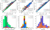 |
Fig. 1 Aperture correction for APEX observation-related tests and measurements. Upper left: global versus beam luminosities calculated for WISE W3 (12 μm; green), ACA (red), and CARMA (blue) detected galaxies. The dotted lines indicate the 2:1, 5:1, and 10:1 loci, respectively. Upper middle: CO(2-1) luminosities from APEX measurements |
![$\[\left(L_{\mathrm{CO}}^{B}\right)\]$](/articles/aa/full_html/2025/07/aa53179-24/aa53179-24-eq3.png)
![$\[\left(L_{12 \mu \mathrm{m}}^{B}\right)\]$](/articles/aa/full_html/2025/07/aa53179-24/aa53179-24-eq4.png)
![$\[L_{\mathrm{CO}}^{G}\]$](/articles/aa/full_html/2025/07/aa53179-24/aa53179-24-eq5.png)
![$\[L_{\text {CO}}^{B}\]$](/articles/aa/full_html/2025/07/aa53179-24/aa53179-24-eq6.png)
![$\[L_{C O}^{G} / L_{C O}^{\mathrm{B}}\]$](/articles/aa/full_html/2025/07/aa53179-24/aa53179-24-eq7.png)
3.2 Physical quantity derivation
The physical quantities defined and used in this paper are substantially consistent with C20, with few modifications.
3.2.1 CO observation-based quantities
For beam quantities from APEX, ACA, and CARMA observations, CO fluxes are derived within a spectral window of 600 km s−1 centred on the systemic velocity of the galaxy, which is measured from the stellar redshift. The CO line velocity-integrated flux density is expressed by the following equation:
![$\[S_{\mathrm{CO}}\left[\mathrm{Jy} \mathrm{~km} \mathrm{~s}{ }^{-1}\right]=\sum_i T_{\mathrm{A}, i}^* \delta v.\]$](/articles/aa/full_html/2025/07/aa53179-24/aa53179-24-eq13.png) (5)
(5)
Here δv = 30 km s−1 is the channel width. While ![$\[T_{\mathrm{A}}^*\]$](/articles/aa/full_html/2025/07/aa53179-24/aa53179-24-eq14.png) is typically measured in K, we converted SCO to Jy km s−1 through a conversion factor between Kelvin and Jansky directly measured by APEX for each observing year using several calibrators13. Since some of our observations span more than a single run, we considered an average of the fiducial conversion factors listed on the APEX website. We used a similar procedure to infer the proper main beam efficiency (ηmb) for a given measurement set, in order to covert
is typically measured in K, we converted SCO to Jy km s−1 through a conversion factor between Kelvin and Jansky directly measured by APEX for each observing year using several calibrators13. Since some of our observations span more than a single run, we considered an average of the fiducial conversion factors listed on the APEX website. We used a similar procedure to infer the proper main beam efficiency (ηmb) for a given measurement set, in order to covert ![$\[T_{\mathrm{mb}}=T_{A}^{*} / \eta_{\mathrm{mb}}\]$](/articles/aa/full_html/2025/07/aa53179-24/aa53179-24-eq15.png) . The median Jy/K conversion estimated in this way is 36, with an interquartile range equal to 2. To calculate the conversion factor for the interferometers, we simply assumed the beam and frequency information provided in the datacube headers. For ACA beam quantities, this factor is equal to 30.1, while for CARMA beam quantities, Jy/K=7.5. Note, however, that those conversion factors are related to the main beam temperature (Tmb) scale, upon which the CARMA and ACA datacubes are provided.
. The median Jy/K conversion estimated in this way is 36, with an interquartile range equal to 2. To calculate the conversion factor for the interferometers, we simply assumed the beam and frequency information provided in the datacube headers. For ACA beam quantities, this factor is equal to 30.1, while for CARMA beam quantities, Jy/K=7.5. Note, however, that those conversion factors are related to the main beam temperature (Tmb) scale, upon which the CARMA and ACA datacubes are provided.
The statistical error for the flux can be measured as
![$\[\epsilon_{\mathrm{CO}}\left[\mathrm{Jy} \mathrm{~km} \mathrm{~s}{ }^{-1}\right]=\sigma_{\mathrm{RMS}} \sqrt{W_{50} \delta v},\]$](/articles/aa/full_html/2025/07/aa53179-24/aa53179-24-eq16.png) (6)
(6)
where σRMS is the standard deviation of the ![$\[T_{\mathrm{A}}^*\]$](/articles/aa/full_html/2025/07/aa53179-24/aa53179-24-eq17.png) variations measured in the first and last 20 line-free channels of each spectrum. As in C20, we used the second moment (σv) calculated in the spectral window selected to measure the emission line to infer
variations measured in the first and last 20 line-free channels of each spectrum. As in C20, we used the second moment (σv) calculated in the spectral window selected to measure the emission line to infer ![$\[W_{50}=\sqrt{8 \log (2)} \sigma_{\mathrm{v}}\]$](/articles/aa/full_html/2025/07/aa53179-24/aa53179-24-eq18.png) . Additionally, we assumed a fiducial W50 = 300 km s−1, which is consistent with the peak of the W50 distributions calculated for APEX, ACA, and CARMA-detected galaxies. The parameter ϵCO is used to provide an upper limit of the flux for non-detected galaxies, where
. Additionally, we assumed a fiducial W50 = 300 km s−1, which is consistent with the peak of the W50 distributions calculated for APEX, ACA, and CARMA-detected galaxies. The parameter ϵCO is used to provide an upper limit of the flux for non-detected galaxies, where ![$\[\mathrm{S} / \mathrm{N}=T_{\mathrm{A} \text {, peak }}^{*} / \sigma_{\mathrm{RMS}}<3\]$](/articles/aa/full_html/2025/07/aa53179-24/aa53179-24-eq19.png) (e.g. SCO < 3ϵCO).
(e.g. SCO < 3ϵCO).
Given the flux, the CO luminosity can be inferred following Equation (3) of Solomon et al. (1997),
![$\[L_{\mathrm{CO}}\left[\mathrm{K} \mathrm{~km} \mathrm{~s}^{-1} \mathrm{pc}^2\right]=3.25 \times 10^7 \frac{D_L^2}{\nu_{\mathrm{obs}}^2(1+z)^3} S_{\mathrm{CO}},\]$](/articles/aa/full_html/2025/07/aa53179-24/aa53179-24-eq20.png) (7)
(7)
where DL is the luminosity distance in Mpc (derived from the stellar redshift, z), νobs is the observed frequency of the emission line in the rest frame in GHz (νobs = 115 GHz for CARMA data, and νobs = 230 GHz for APEX and ACA data), and SCO is the CO velocity-integrated flux derived using Equation (5).
This formula set is directly used to infer beam quantities. After that, in the case of APEX data, global LCO are derived using the aperture correction given by Equation (4). Global fluxes are retroactively calculated from global luminosities. In this case, we assumed that the global and beam ϵCO are equivalent. For CARMA and ACA data, we considered the published SCO values to infer global luminosities (following Equation (7)).
From the CO luminosity, the molecular gas mass, Mmol, can be measured by assuming a CO-to-H2 conversion factor, αCO:
![$\[M_{\mathrm{mol}}\left[\mathrm{M}_{\odot}\right]=\alpha_{\mathrm{CO}} L_{\mathrm{CO}}.\]$](/articles/aa/full_html/2025/07/aa53179-24/aa53179-24-eq21.png) (8)
(8)
More information regarding the αCO model adopted here is given in the next section.
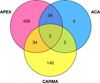 |
Fig. 2 Number of galaxies within the iEDGE observed by the different telescopes represented as a Venn diagram. Objects solely observed by APEX eventually constitute 64% of the final database, and CARMA data add up to 22% of the database. The rest of the targets have been observed by multiple telescopes. |
3.2.2 IFU observation-based quantities
As in C20, we used Hα, Hβ, [OIII] λ5007, [NII] λ6583 flux maps, FHα, FHβ, F[OIII], F[NII], respectively; the Hα equivalent width, WHα, and the stellar mass surface density maps; all collected in pseudo-cubes, a term referring to the reduced data products produced by the PIPE3D pipeline (Sánchez et al. 2016c,b). These pseudo-cubes are made of spatially resolved maps whose each spaxel contains physical quantities such as emission line fluxes, equivalent widths, and stellar mass surface densities derived from the analysis of CALIFA spectra. PIPE3D applies the GSD156 simple stellar populations (SSP) library (Cid Fernandes et al. 2013) to perform a spaxel-wise fit of the stellar population model on spatially rebinned V-band data cubes. This model is applied to calculate the stellar mass density value within each spaxel. The ionised gas data cube is inferred by subtracting the stellar population model from the original cube. Each of the 52 sets of emission line maps is obtained, calculating flux intensity, centroid velocity, velocity dispersion, and equivalent width for every spectrum. The maps included in the PIPE3D cubes are used to calculate integrated star formation rates (SFRs), stellar masses (M*), and CO-to-H2 conversion factors (αCO).
For the extinction-corrected SFR map derivations, we followed the procedure included in Villanueva et al. (2024), which is largely similar to C20 but with a few modifications. In general, we applied the Balmer decrement method for each spaxel in the CALIFA map to calculate the nebular extinction
![$\[A_{\mathrm{H} \alpha}[\mathrm{Mag}]=\frac{K_{\mathrm{H} \alpha}}{0.4\left(K_{\mathrm{H} \beta}-K_{\mathrm{H} \alpha}\right)} \times \log \left(\frac{F_{\mathrm{H} \alpha}}{2.86 F_{\mathrm{H} \beta}}\right),\]$](/articles/aa/full_html/2025/07/aa53179-24/aa53179-24-eq22.png) (9)
(9)
where the coefficients KHα = 2.53 and KHβ = 3.61 follow the Cardelli et al. (1989) extinction curve (see also Catalán-Torrecilla et al. 2015).
![$\[\mathrm{SFR}\left[\mathrm{M}_{\odot} ~\mathrm{yr}^{-1}\right]=8 \times 10^{-42} L_{\mathrm{H} \alpha} \times 10^{A_{\mathrm{H} \alpha}},\]$](/articles/aa/full_html/2025/07/aa53179-24/aa53179-24-eq23.png)
as indicated by Kennicutt (1998), which assumes the Salpeter initial mass function (Salpeter 1955), where LHα is the Hα luminosity calculated as LHα [erg s−1]=4πD2FHα [erg s−1 cm−2], with the distance to the target DL in cm.
To obtain the final SFR maps, a series of masks is also considered. First of all, we masked all spaxels where S/N< 3 for Hα and Hβ. Additionally, we imposed a mask based on the WHα, where we considered only spaxels where WHα ≥ 6 Å, as those are the only ones consistent with hydrogen ionisation from recent star formation activity (see Cid Fernandes et al. 2010; Sánchez et al. 2018; Kalinova et al. 2021). Furthermore, we applied a conservative mask that takes into account the spaxels where the ionisation is influenced by the AGN activity rather than purely by star formation. In essence, we removed all spaxels that lie above the BPT diagram (Baldwin et al. 1981) demarcation line given by Kewley et al. (2001) in their Equation (5). We also imposed several conditions to be fully consistent with Villanueva et al. (2024) derivations. We considered a minimum FHα/FHβ = 2.86, therefore we imposed FHα/FHβ ≡ 2.86 for the spaxels where FHα/FHβ < 2.86. For spaxels where FHβ is masked, therefore AHα not defined, we imposed AHα equal to the median of AHα, calculated where FHβ is finite (as also assumed in Barrera-Ballesteros et al. 2020).
Finally, to obtain the integrated global SFRs, we spatially co-added the spaxels within the SFR maps, derived in Equation (10) (namely SFRG=∑i SFRi, where i runs across the spaxels of the map), while for the beam SFRs, before the summation, the maps are multiplied by the tapering function map, WT (basically SFRB=∑i SFRi × WT,i).
Similarly, the global stellar mass, M*, G=∑i M*,i, is given by the summation over the whole map directly included in the PIPE3D pseudo-cube. The stellar mass within the APEX beam, M*, B=∑i M*,i × WT,i, is obtained in the same way as SFRB by the summation of the stellar masses from the spaxels, weighted by the tapering function WT.
Additionally, we used nebular emission lines information to infer the gas-phase metallicity, which is the fundamental parameter upon which αCO depends on. We measured the gas-phase metallicity using the O3N2 method by Pettini & Pagel (2004):
![$\[12+\log \left(\frac{\mathrm{O}}{\mathrm{H}}\right)=8.73-0.32 \times \log \left(\frac{F_{[\mathrm{OIII}]}}{F_{\mathrm{H} \beta}} \frac{F_{\mathrm{H} \alpha}}{F_{[\mathrm{NII}]}}\right).\]$](/articles/aa/full_html/2025/07/aa53179-24/aa53179-24-eq24.png) (11)
(11)
Nonetheless, Pettini & Pagel (2004) O3N2 calibrator is obtained from HII regions. Therefore, we have to impose a cut on the metallicity maps based on WHα in order to exclude all non-star-forming regions (e.g. where WHα < 6 Å). To recover the metallicity in those regions, we created a map based on the metallicity-stellar mass relation (MZR). In particular, we used the model inferred from CALIFA data by Sánchez et al. (2017)
![$\[12+\log \left(\frac{\mathrm{O}}{\mathrm{H}}\right)=8.73+0.01 \times(x-3.50) \exp (-(x-3.50)),\]$](/articles/aa/full_html/2025/07/aa53179-24/aa53179-24-eq25.png) (12)
(12)
where x = log(M*/M⊙) − 8.0. This relation predicts the metallicity at 1 Re through the global stellar mass of the galaxy, M*. We built a radial metallicity map assuming a universal metallicity gradient −0.1 dex/Re (see Sánchez et al. 2014 and Sun et al. 2020).
Several metallicity calibrations have been proposed (see Sánchez 2020, for example). Here, we adopt the Pettini & Pagel (2004) calibration because it yields an oxygen abundance close to the Solar value assumed in this work (8.69; Allende Prieto et al. 2001). We emphasise, however, that the Solar metallicity is subject to uncertainties and revisions (e.g. Lodders 2003; Asplund et al. 2009), and our choice is intended to ensure a reasonable consistency with the assumed value. We explore the implications regarding the usage of these ‘combined’ metallicity maps versus the ‘emission lines’ – only derived metallicity maps on the derived αCO(1–0) values in Appendix A.
Beam median gas-phase metallicities are calculated assuming the weights given by the Gaussian filter, WT, on the combined metallicity map. Using this method, we obtain a median of 8.65 dex from the full galaxy sample with an inter-quartile range of 0.12 dex. The median beam metallicity with respect to the Solar metallicity is ![$\[Z_{\mathrm{B}}^{\prime}=0.92\]$](/articles/aa/full_html/2025/07/aa53179-24/aa53179-24-eq26.png) . Instead, the global metallicity is measured simply as the median across the full metallicity map. This gave us a median global metallicity across the full sample consistent with the beam metallicity, i.e. equal to 8.65 dex, with an interquartile range equal to 0.08. Similarly, we obtained
. Instead, the global metallicity is measured simply as the median across the full metallicity map. This gave us a median global metallicity across the full sample consistent with the beam metallicity, i.e. equal to 8.65 dex, with an interquartile range equal to 0.08. Similarly, we obtained ![$\[Z_{\mathrm{G}}^{\prime}=0.80\]$](/articles/aa/full_html/2025/07/aa53179-24/aa53179-24-eq27.png) .
.
As in C20, here we assumed a variable αCO(1–0) based on Bolatto et al. (2013), Equation (31)
![$\[\alpha_{\mathrm{CO}(1-0)}\left[\mathrm{M}_{\odot}\left(\mathrm{K} \mathrm{~km} \mathrm{~s}^{-1} \mathrm{pc}^2\right)^{-1}\right]=2.9 \exp \left(\frac{0.4}{Z^{\prime}}\right) \times\left(\frac{\Sigma_*}{100 \mathrm{M}_{\odot} ~\mathrm{pc}^{-2}}\right)^{-\gamma},\]$](/articles/aa/full_html/2025/07/aa53179-24/aa53179-24-eq28.png) (13)
(13)
where Z′ is the gas-phase metallicity relative to solar metallicity and Σ* is the stellar mass surface density measured at each pixel in the CALIFA data and γ = 0.5 where Σ* > 100 M⊙ pc−2 or γ = 0 otherwise. To avoid iterative solving, here we simply considered that Σtotal ≡ Σ*, since for our sample of galaxies, the gas mass surface density is generally one order of magnitude lower than the stellar mass surface density. Also, ![$\[\Sigma_{\mathrm{GMC}}^{100}\]$](/articles/aa/full_html/2025/07/aa53179-24/aa53179-24-eq29.png) , the Giant Molecular Cloud (GMC) molecular gas mass surface density in units of 100 M⊙ pc−2, does not appear in Equation (13) as we assume
, the Giant Molecular Cloud (GMC) molecular gas mass surface density in units of 100 M⊙ pc−2, does not appear in Equation (13) as we assume ![$\[\Sigma_{\mathrm{GMC}}^{100}=1\]$](/articles/aa/full_html/2025/07/aa53179-24/aa53179-24-eq30.png) therefore, considering that GMC molecular gas mass surface density inner regions of nearby galaxies and Milky Way is largely consistent with 100 M⊙ pc−2 (see Sun et al. 2018; Colombo et al. 2019; Rosolowsky et al. 2021). For low-mass galaxies (with M* < 109 M⊙) where the MZR is not defined and the optical emission lines remain undetected, we assumed Z′ = 1, which is the typical value for local Universe galaxies with Milky Way mass. In Equation (13), αCO is calculated across the whole CALIFA map; within the APEX beam aperture, we used the weighted median from the CO-to-H2 conversion factor map, αCO(1–0), B, where the weights for each spaxel are given by the tapering function, WT. The global αCO(1–0), G is simply the median across the αCO(1–0) map.
therefore, considering that GMC molecular gas mass surface density inner regions of nearby galaxies and Milky Way is largely consistent with 100 M⊙ pc−2 (see Sun et al. 2018; Colombo et al. 2019; Rosolowsky et al. 2021). For low-mass galaxies (with M* < 109 M⊙) where the MZR is not defined and the optical emission lines remain undetected, we assumed Z′ = 1, which is the typical value for local Universe galaxies with Milky Way mass. In Equation (13), αCO is calculated across the whole CALIFA map; within the APEX beam aperture, we used the weighted median from the CO-to-H2 conversion factor map, αCO(1–0), B, where the weights for each spaxel are given by the tapering function, WT. The global αCO(1–0), G is simply the median across the αCO(1–0) map.
The CO-to-H2 conversion factor given by Equation (13) is directly applicable to calculate the molecular gas mass for CARMA observations, through Equation (8). However, APEX and ACA observed the molecular gas through the 2–1 transition of 12CO. Generally, a constant CO(2-1)-over-CO(1-0) emission line ratio (R21 ~ 0.65, Leroy et al. 2022) is assumed to convert from the CO(1-0)-to-H2 to the CO(2-1)-to-H2 conversion factor (e.g. αCO(2–1) = αCO(1–0)/R21). Nevertheless, den Brok et al. (in prep.) observed that, on kiloparsec scales, R21 is tightly correlated to ΣSFR inferred from Hα, and the relation appears to be environment-independent (see also Narayanan & Krumholz 2014; Leroy et al. 2022; den Brok et al. 2023). In particular, they measured (their Equation (4))
![$\[\log _{10}\left(R_{21}\right)=0.12 \log _{10}\left(\frac{\Sigma_{\mathrm{SFR}}}{\mathrm{M}_{\odot} ~\mathrm{yr}^{-1} ~\mathrm{kpc}^{-2}}\right)+0.06.\]$](/articles/aa/full_html/2025/07/aa53179-24/aa53179-24-eq31.png) (14)
(14)
We applied this relation to calculate R21 maps from ΣSFR maps. However, we used only spaxels where ΣSFR > 10−3 M⊙ yr−1 kpc−2 to be consistent with the range of values considered by den Brok et al. (in prep.). As for αCO, we assumed a global R21, G as the median across the R21 map, while R21, B is again the median of R21 map, where each spaxel is weighted by the tapering function WT. Given this, αCO(2–1), G = αCO(1–0), G/R21, G and αCO(2–1), B = αCO(1–0), B/R21, B.
Through these parameters, we had access to two fundamenttal quantities to study the star formation quenching across our galaxy sample, the star formation efficiency,
![$\[\mathrm{SFE}=\frac{\mathrm{SFR}}{M_{\mathrm{mol}}},\]$](/articles/aa/full_html/2025/07/aa53179-24/aa53179-24-eq32.png) (15)
(15)
and the molecular gas mass-to-stellar mass ratio, or molecular gas fraction,
![$\[f_{\mathrm{mol}}=\frac{M_{\mathrm{mol}}}{M_*}.\]$](/articles/aa/full_html/2025/07/aa53179-24/aa53179-24-eq33.png) (16)
(16)
4 Results
4.1 Comparisons between luminosities observed by different telescopes
Several targets in our sample have been observed by multiple telescopes, namely, 58 galaxies have been observed by both APEX and ACA, and 36 galaxies have been observed by both APEX and CARMA. This gives the opportunity to evaluate the global luminosities inferred for APEX galaxies and the performance of the aperture correction. Luminosities are calculated following the indications in Section 3.2.
The relations between beam luminosity inferred from APEX and ACA, and APEX and CARMA observations are shown in Fig. 3 (upper row). Generally, ACA beam luminosities follow APEX beam luminosities, with a smaller scatter compared to the other relations presented in this section. APEX luminosities are, on average, ~27% higher than ACA luminosities. This can be due to differences in calibration, for example (as noticed by Villanueva et al. 2024). Additionally, ACA data do not include total power observations, as the largest recoverable scale is basically the optical radius of the CALIFA galaxies (roughly 25 arcsec). However, we cannot rule out the possibility that a certain fraction of flux is filtered out in some galaxies. Larger deviations are observed for objects barely detected by ACA or highly inclined ones, for which the APEX beam extends further away from the galactic discs. Similarly, the luminosity measured for the same galaxies by CARMA and APEX is, on average, equal. However, while both ACA and APEX observed the CO(2-1) emission, CARMA observed the CO(1-0) emission. The typical CO(2-1)-to-CO(1-0) ratio, R21, inferred from nearby spiral galaxies is ~0.65 (see Section 3.2.2). Here, instead, we measured a median R21 ~ 1 in the centre of our galaxies. This higher-than-expected value can be attributed to differences in calibration between the two telescopes, however, the missing flux in the interferometric observations of CARMA might also play a role in increasing the ratio. As for the ACA sample, tests conducted to compare the CO fluxes between CARMA and COLDGASS14 data did not reveal significant flux filtering, however, this cannot be completely excluded as CARMA data do not include a proper short-spacing correction (e.g. single-dish observations; see Bolatto et al. 2017, their Section 3.2). Additionally, the three surveys have intrinsically been designed to reach different sensitivities. This is reflected in the upper limits of the luminosities. Indeed, considering the same galaxies, luminosity upper limits from APEX are more than 0.5 dex higher than the luminosity upper limits from ACA (Fig. 3, upper left panel). On the opposite end, the luminosity upper limits from CARMA are 0.5 dex higher than the ones from APEX.
The comparison between the global luminosities inferred from the three telescopes is shown in Fig. 3 (lower row panels). For this analysis, we do not consider the upper limits, as those are dependent upon the noise levels (σRMS; Equation (6)), which in turn are dependent upon the (heterogeneous) channel widths of the original set of data. The global luminosities obtained through the aperture correction procedure described in Section 3.1.3 are largely similar to the global luminosities calculated from ACA data. Still, on average, APEX luminosities appear 16% higher than ACA-inferred luminosities. Besides the effects that we described above regarding the beam-wise luminosity analysis, this discrepancy can also be due to the masking procedure adopted for ACA (and WISE W3) data that might provide slightly different fluxes based on the chosen noise threshold. However, it is important to note that the ratio between APEX and ACA global luminosities is roughly consistent with the same ratio measured for beam luminosities, meaning that the 12 mum-based aperture correction provides a robust recovery of the global flux for APEX observations. In essence, this test further validates our chosen aperture correction method for APEX galaxies. Instead, CARMA global luminosities appear, on average, 18% higher than APEX global luminosities. Again, several effects could be involved in this discrepancy, together with the fact that the fluxes from the smooth masking procedure tend to be higher than the ones obtained from the more conservative dilated masking procedure (see Bolatto et al. 2017 for further details). In this aspect, however, from the global luminosities, we measure a median R21 = 0.82, closer to the canonical R21 = 0.65 value. Summarising, the comparison between observations from APEX, ACA, and CARMA demonstrates overall consistency in inferred CO luminosities, with systematic offsets possibly given by differences in calibration, sensitivity, and spatial filtering, and confirms the robustness of our aperture correction method for APEX data.
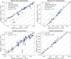 |
Fig. 3 Comparison between beam-wise (top panels) and global luminosities (bottom panels) from ACA and APEX (left panels) and from CARMA and APEX (right panels). The blue circles indicate galaxies detected (with S/N > 3) from both telescopes, yellow arrows indicate galaxies detected only by ACA or CARMA, the green arrows indicate galaxies detected only by APEX, and the red crosses show galaxies not detected by both telescopes. For non-detections, luminosities are given as upper limits. For global luminosities, we show only the detections from both telescopes (see the text for further details). The black solid lines mark the 1:1 locus. The magenta dashed line has a unitary slope and an intercept equal to the median ratio between the x – and the y-quantities. In addition, in the left panels, the dotted black line marks the location where the CO(2-1)-to-CO(1-0) ratio, R21 = 0.65. The grey dashed lines have a unitary slope and are separated by 0.5 dex. |
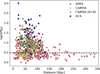 |
Fig. 4 Detection distance bias shown as the beam S/N vs the distance to the galaxies, for APEX- (red), CARMA- (yellow), CARMA (D+E)- (green empty), ACA- (blue) observed galaxies. The black dashed line indicates a S/N=3 that marks the separation between detections and nondetections. Non-detections (observations with S/N<3) starkly decrease from a distance >130 Mpc and are all related to APEX observations. |
4.2 Distance bias
Although CALIFA galaxies are all local objects (having a maximum redshift equal to 0.08) and are diameter-selected, some distance bias can be present in our database. In Fig. 4, the beam S/N ratio of the CO observation versus the distance to the galaxies is shown for the different telescopes constituting the final sample. The bulk of objects is observed within a distance of 150 Mpc. In this distance range, the number of the detected galaxies is a factor 2.4 larger than the number of non-detected galaxies. However, for distances >130 Mpc, the galaxies are mostly non-detected, and they are all observed by APEX. Nevertheless, those are only 50 targets or 8% of the sample. This concludes that a significant distance detection bias is absent in our database.
4.3 iEDGE sample statistics
4.3.1 Definition of the consolidated sample
The iEDGE that we are presenting here consists of galaxies which have been observed by multiple telescopes. The Venn diagram represented in Fig. 2 summarises the sample overlaps. The majority of targets (~64%) in the database have been observed only by APEX, while another ~22% has been uniquely observed by CARMA. Almost all ACA galaxies (58 targets) were previously observed by APEX. Additionally, 34 targets have been observed by both APEX and CARMA, while 2 galaxies (UGC08781 and UGC10972) have been observed by all three telescopes. If we restrict the CARMA data to the D+E targets, the distribution of the target number changes slightly. CARMA D+E galaxies constitute ~16% of the database, while the overlap with APEX is constituted by 26 galaxies. With ACA, we did not reobserve D+E targets (meaning there is no overlap between the D+E CARMA and ACA), but ACA observed 2 CARMA E-only galaxies (NGC 2449, UGC05396), which have not been observed by APEX.
The distribution of galaxies across the SFR-M* diagram is typically used as a standard diagnostic for sample characterisation; therefore, in Fig. 5 (left), we present the position of the various galaxy samples within our database on this diagram. It is clear that the APEX sample covers the parameter space defined by the two variables, and it is more representative of the CALIFA sample compared to the others. In particular, while CARMA galaxies extend from the star formation main sequence region to the retired region, quenched galaxies are mostly observed by the E-configuration only, while D+E targets are constrained to the SFMS. ACA targets seem to follow a distribution similar to the CARMA E targets. The distribution of the targets on the SFR-M* diagram considering their S/N is illustrated in Fig. 5 (right). It is interesting to notice that while the number of detected galaxies is generally found along the SFMS, several non-detections are also observed in the same region. Still, there are several detections in the green valley and the retired region of the diagram.
Given the overlaps described at the beginning of this section, in the analyses adopted in the paper, we have used a set of criteria to define our ‘consolidated’ sample of unique galaxies. For consistency, we prioritised APEX data and used CARMA data only if the targets had not been covered by APEX. We used ACA data instead of APEX data in case the latter showed better S/N compared to the former. We had, therefore, included 454 APEX galaxies, 47 ACA galaxies, 100 CARMA (D+E) galaxies, and 42 CARMA (E) galaxies. Nevertheless, we verified that for galaxies observed by multiple telescopes (64 objects), the mean ratio between these measurements and the corresponding values in the consolidated sample remains close to unity (on average). The most significant discrepancies (up to a factor of 2) occur when the S/N of the measurements contributing to the mean is either low (S/N ~ 3–4, as in the case of NGC 0155) or when the individual measurements exhibit substantial differences due to the S/N of the detections (e.g. UGC 08781). Finally, the description of all quantities included in this release of the database is in Table C.1.
4.3.2 Star formation rate and stellar mass completeness
The statistics of SFR and M*-related properties for our consolidated samples compared with the parental CALIFA sample are collected in Fig. 6. Our CO-detected targets showed a stellar mass, which generally missed the low and high mass tails of the CALIFA distribution, and they are generally limited to 8.5 < log(M*/[M⊙]) < 12.5. The full iEDGE sample contains larger fractions of data below and above those limits, but they are not detected. Regarding the SFR, our detections are representative of the −1 < log(SFR/[M⊙ yr−1]) < 1 range of the CALIFA parental distribution. Several targets are observed below −1 < log(SFR/[M⊙], but they are not detected in CO. This might simply reflect the fact that these targets are quenched due to low molecular gas fractions. This evidence is reflected in the sSFR histogram (see Fig. 6). Although galaxies with low sSFR are included in our sample, the iEDGE misses objects with log(sSFR/[yr−1]) > −9. Considering the logarithmic distance from the SFMS fit (for which we assumed the Cano-Díaz et al. 2016 model: log(SFR/[M⊙ yr−1]) = −8.34 + 0.81 log(M*/[M⊙])), it seems that these high sSFR galaxies are objects more than 1 dex away from the SFMS, or that the iEDGE sample generally missed the very high star-forming galaxies (possibly starburst, where ΔSFMS > 1) present in the CALIFA parental sample. Additionally, the database does not contain the few low (ΔSFMS < −4) targets present in the CALIFA sample. This said, the iEDGE is largely representative of the CALIFA parental sample considering sSFR and ΔSFMS, which are fundamental to studying star formation quenching in the galaxies.
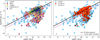 |
Fig. 5 SFR-M* diagrams defined by the different samples considered in this paper (left panel): full CALIFA (cyan hexagons), and galaxies observed in CO lines by APEX (red circles), CARMA (yellow diamonds), CARMA (D+E galaxies only, empty green diamonds), ACA (blue squares). In the right panel, the red circles represent CO-detected galaxies (with S/N > 3), while the black dots show CO non-detections (with S/N < 3). In both panels, the black line shows Cano-Díaz et al. (2016) the SFMS model with the uncertainties (dotted lines). The dashed purple line indicates the green valley boundary position defined in C20, which is located 3σ (equal to 0.20 dex as in Cano-Díaz et al. 2016) from the SFMS. APEX targets extend from the SFMS to the retired regions, better representing the CALIFA galaxies in this diagram. |
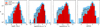 |
Fig. 6 Histograms across samples (full CALIFA, cyan bars; galaxies in the full iEDGE sample, black empty bars; CO detected galaxies in the iEDGE, red bars) related (from left to right) to M*, SFR, specific SFR (sSFR=SFR/M*), and logarithmic distance from the SF main sequence (ΔSFMS). Similarly to CALIFA, iEDGE spans a representative range of SFR, M*, and related values. However, CO detections decrease at low sSFR and ΔSFMS values. |
4.3.3 R21 and αCO(1-0) distributions
As described in Section 3.2, the IFU data provide a way to model several quantities that are generally assumed when multiple CO transition and isotopologue emissions are not available to properly infer the H2 column density, namely R21 and αCO(1–0). Here, for each galaxy in the sample, we assumed R21, calculated through its correlation with the SFR surface density (see Equation (14)). The distribution of this (global and beam) parameter is shown in Fig. 7 (left) and ranges between 0.5 and 0.85 (with a single object showing R21 > 1). In detail, we obtained a median R21, G = 0.60 with an interquartile range of 0.08 and a median R21, B = 0.62 with an interquartile range equal to 0.07. The medians, in particular, are consistent with the R21 values measured across galactic discs via direct comparison of the CO(2-1) and CO(1-0) emission of 0.6–0.70 (see Yajima et al. 2021; den Brok et al. 2021; Leroy et al. 2022). In Section 4.1, we calculated a median R21 = 0.82 for the galaxies for which we possess both APEX and CARMA data. However, several objects showed luminosities ratios close to the canonical R21 = 0.65, with other galaxies deviating from this value. Nevertheless, R21 ~ 0.8 are not uncommon in the literature, as reported by several studies (Braine et al. 1993; Saintonge et al. 2017; Cicone et al. 2017).
The distribution of global and beam CO(1-0)-to-H2 conversion factors (αCO(1–0)) modelled from the gas-phase metallicity and the stellar mass surface density (following Equation (13)) is shown in Fig. 7 (right). Together, histograms spread between ~1.5 and 11. In detail, we obtained a median αCO(1–0), B = 4.07 M⊙ (K km s−1 pc2)−1, with an interquartile range equal to 1.46 M⊙ (K km s−1 pc2)−1; and a median αCO(1–0), G = 4.70 M⊙ (K km s−1 pc2)−1, with an interquartile range equal to 0.45 M⊙ (K km s−1 pc2)−1. Both estimations are statistically consistent with the Milky Way generally assumed value αCO(1–0) = 4.35 M⊙ (K km s−1 pc2)−1. We discuss further implications on the assumed method to calculate αCO(1–0) and the dependences of αCO(1–0) on metallicity and stellar mass surface density in Appendix A.
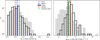 |
Fig. 7 Distributions of the inferred CO(2-1)-to-CO(1-0) ratio (R21, left) and CO(1-0)-to-H2 conversion factors (αCO(1–0), right). These quantities are derived using IFU maps from models described in Equations (13) and (14) (for αCO(1–0) and R21, respectively). Histograms show median R21 and αCO(1–0) calculated across the full maps (global, empty black histograms) and tapered maps (beam, grey histograms). The red (blue) dashed lines indicate the median of the global (beam) quantities, while the green dash-dotted lines show the typical values adopted for star-forming galaxies in the local Universe (e.g. R21 = 0.65 and αCO(1–0) = 4.35 M⊙ (pc2 K km s−1)−1). Regarding R21, we measured medians (depending on the coverage) generally lower than the average values observed in nearby galaxies. The αCO(1–0) values span an order of magnitude, with lower conversion factors measured within the galaxy centres. This is consistent with the fact that galaxies exhibit a declining metallicity trend with respect to the galactocentric radius, hence showing lower αCO(1–0) in their centre (see also Appendix A). |
4.4 Fundamental scaling relations for star formation
The scaling relations between SFR, M*, and Mmol can provide valuable insight into the evolution of galaxies. With the 643 galaxies included in the iEDGE database, we can accurately represent them (Fig. 8). For this analysis, we colour-encoded the diagram based on the median Hα equivalent width across the full maps, ⟨WHα⟩ (Fig. 8, upper row) and on their morphology (Fig. 8, lower row). Generally, star-forming, spiral galaxies and retired, early-type galaxies form well-distinguishable sequences across the three diagrams. In the following, we also consider the nuclear activity of the galaxies. To establish if a galaxy hosts an AGN, we adopted the scheme by Kalinova et al. (2021) (but see also Cid Fernandes et al. 2010; Sánchez et al. 2014; Lacerda et al. 2018, 2020), who considered the three Baldwin-Phillips-Terlevich (BPT; Baldwin et al. 1981) diagnostic diagrams that use the [OIII], [SII], [OI] and [NII] line ratios with respect to the Hα and Hβ lines. In this scheme, if three spaxels (covering a CALIFA PSF) within 0.5 Re are found in the Seyfert region of at least 2 BPT diagrams, the galaxy is considered a candidate AGN-host. Nevertheless, the spaxels need to show a WHα ≥ 3 Å to be considered as a weak AGN (wAGN) host galaxy, or a WHα ≥ 6 Å to be considered as a strong AGN (sAGN) host galaxy.
The standard appearance of the SFR–M* diagram (e.g. Brinchmann et al. 2004; Daddi et al. 2007; Catalán-Torrecilla et al. 2015; Renzini & Peng 2015; Cano-Díaz et al. 2016; Sánchez et al. 2018; Sánchez 2020) is faithfully reproduced by the iEDGE data (Fig. 8, left), with galaxies across the SFMS having ⟨WHα⟩ ≥ 6 Å in general, galaxies in the red sequence showing typically ⟨WHα⟩ ≤ 3 Å, and green valley targets bounded by these two limits. Still, we found several galaxies having large ⟨WHα⟩ values up the retired region. As it has been established several times, WHα, along side the colour, is a faithful proxy of the star-forming properties of galaxies. Indeed, finding ⟨WHα⟩ ≥ 6 Å indicates hydrogen ionisation due to star formation activity (e.g. HII regions), while ⟨WHα⟩ ≤ 3 Å indicates ionisation due to the old stellar population (e.g. Sánchez 2020; Kalinova et al. 2021). Therefore, it is not surprising to find that spiral and star-forming galaxies, on the one hand, and retired spheroids, on the other hand, are characterised by those values of WHα. Active galaxies mainly occupy the high mass region of the diagram (typically M* > 1010 M⊙) and they are constrained between the SFMS fit and the red sequence (where SFR < 10−2 M⊙ yr−1). Across the diagram, spiral galaxies appear to dominate the SFMS and the green valley, while the retired region is constituted by early-type galaxies. Still, we observe that some S0-type objects have high SFR. Barred galaxies are mostly observed above the SFMS fit. In the SFR–Mmol relation (Fig. 8, middle) star-forming galaxies (with ⟨WHα⟩ ≥ 6 Å) are organised across a line defined by a molecular depletion time τdep = 2 Gyr, which is considered as the typical depletion time for star-forming galaxies (e.g. Bigiel et al. 2011; Rahman et al. 2012; Leroy et al. 2013; Utomo et al. 2017; Sun et al. 2023). However, we also noticed a deviation towards higher SFR (therefore lower τdep) for star-forming galaxies with log(Mmol/[M⊙]) ~ 8. This deviation might be driven by low-mass galaxies, while the most gas-rich objects appear well-organised across the 2 Gyr line. The same deviation can be noticed in Villanueva et al. (2021) (see their Fig. 7), who reproduced the same plot using ACA and CALIFA data. This region is clearly dominated by spiral galaxies (Fig. 8, middle bottom), although several S0 objects are observed across the region. This is not uncommon, though. Several early studies have found early-type galaxies with SFE comparable to spirals (e.g. Lees et al. 1991; Wiklind et al. 1995; Combes et al. 2007). The equivalent of the green valley in this diagram is not clearly noticeable, as galaxies with 3 < ⟨WHα⟩ < 6 Å look to be distributed among the star-forming ones. Instead, retired targets appear to be well separated from the rest, forming an independent ‘sequence’ apparently characterised by τdep ~ 50–100 Gyr. These depletion times are consistent with the value measured for retired targets in the xCOLDGASS sample (Saintonge et al. 2017). This sequence appears to be formed solely by early-type objects (E and SO). Nevertheless, it is difficult to provide a robust definition of this sequence as many targets are non-detected, and we showed only an upper limit for these targets in this diagram. Active galaxies are organised with generally high molecular gas mass and SFR (Mmol > 109 M⊙ and SFR < 10−1 M⊙ yr−1, respectively). Barred galaxies are located mainly above the line that defined the τdep = 2 Gyr. In the rightmost panels of Fig. 8, the logarithmic Mmol − M* relationship is displayed. As in the previous diagrams, sequences for the star-forming and retired galaxies are well defined, while the transitional region (the equivalent of the ‘green valley’ in the SFR–M* relation) is not clearly distinguishable. In particular, the sequence for galaxies dominated by star formation is characterised by fmol ~ 0.1, even if galaxies above and below log(M*/[M⊙] ~ 10) show somehow fmol below and above this value. Instead, the retired region fmol is at least below 0.01. This result is consistent with the measurements from the ATLAS3D survey (Young et al. 2011) reanalysed by Saintonge & Catinella (2022). As noticed before, the active galaxies are generally located at the high Mmol and M* ends of the diagram (see also Sánchez et al. 2018). Spiral galaxies dominate the ‘molecular gas main sequence’ of the diagram, while early-type objects are organised across the retired galaxy region.
Our results are qualitatively consistent with the kiloparsec-scale resolved analyses conducted by the EDGE-CALIFA and ALMaQUEST projects on the same topic. Both star-forming galaxies (Bolatto et al. 2017; Utomo et al. 2017; Lin et al. 2019; Baker et al. 2022; Villanueva et al. 2024) and individual star-forming spaxels (Ellison et al. 2021b,a; Lin et al. 2022) follow well-defined sequences in the resolved SFR–Mmol and Mmol–M* diagrams. In contrast, spaxels in green valley and retired systems (Lin et al. 2022; Villanueva et al. 2024), as well as retired spaxels specifically (Ellison et al. 2021a; Lin et al. 2022), exhibit systematically lower SFE and fmol compared to their star-forming counterparts. This confirms the conclusions of Sánchez (2020), who demonstrated that global and kiloparsec-scale measurements follow statistically consistent scaling relations and extend them to the quiescent regime, where both global and local measurements appear to trace the same underlying relations.
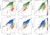 |
Fig. 8 Star formation scaling relations studied here colour-coded by the median equivalent width of Hα (WHα, upper row) and morphology (lower row), from left to right SFR-M*, SFR-Mmol, and Mmol − M*. In the left panel, the elements follow Fig. 5; additionally, the dotted lines are spaced of 3σ from each other. In the middle panel, the black solid line indicates a constant molecular depletion time τdep = 2 Gyr, additionally, dotted lines show constant τdep from (top to bottom) 10−5 to 107 Gyr. In the right panel, the black line indicates a constant molecular gas-to-stellar mass fmol = 0.1; additionally, the dotted lines show constant fmol from (bottom to top) 10−5 to 104. The triangles in the middle and right panels illustrate galaxies for which upper limits for the molecular gas mass are used. At the bottom right of each panel the typical (median) uncertainty for the quantities is shown. In the upper row, the pentagons show the positions of the wAGN-hosts in the sample, while the stars show the positions of sAGN-hosts. In the lower row, the dark blue dots show the locations of the SAB/SB galaxies. Spiral star-forming galaxies on the one hand and early-type retired galaxies on the other hand describe well-defined relationships across the three diagrams. |
4.5 Global versus inner galaxy behaviours of star formation efficiency and molecular gas fraction
The database that we constructed, including both beam and global measurements, allows us to study how the overall behaviours of star formation efficiency (SFE) and molecular gas fraction (fmol) compare with their values in the galaxy inner regions (typically within 1 Re). The results of this analysis are reported in Fig. 9, where global versus beam SFE and fmol are shown colour-encoded for ΔSFMS and the galaxy morphology. Generally, both fmol and SFE decrease by several orders of magnitude from spirals to early-type galaxies. However, while the fraction of molecular gas is spatially constant across the galaxies, the inner SFE is lower compared to the global SFE, especially for passive objects.
In particular, the SFEG is slightly shifted towards higher values compared to SFEB but is still well represented by the 1:1 relation in star-forming spirals, the relation between SFEG and SFEB is flatter across retired, E-S0 galaxies (left panels of Fig. 9). In these systems, the inner regions form stars at a rate that is (roughly) 10 times lower than the global value. This trend shift appears to happen for galaxies of about 1.5–2 dex away from the SFMS (e.g. having ΔSFMS ~ −1.5 ÷ −2). The flatter relation is less defined for elliptical galaxies (which are mostly non-detected), but it is quite clear for the lenticular galaxies. The same behaviour is not observed in fmol diagrams (right panels of Fig. 9) where fmol, G and fmol, B are consistently scattered (or ~1 dex) across the 1:1 relation from the spiral, star-forming galaxies to the retired, early-type systems. This means that the availability of molecular gas does not significantly vary across the galactic discs. Therefore, the reason for low SFE does not seem to be connected with the scarcity of molecular gas in the inner galactic regions but to a reduced SFR. This is a clear manifestation of the inside-out quenching observed in nearby galaxies (e.g. González Delgado et al. 2016; Ellison et al. 2018; Bluck et al. 2019; Kalinova et al. 2021, 2022), although with our database, we cannot robustly separate inner and outer galaxy regions. Even from the currently available spatially resolved data, explaining whether variations of fmol or SFE cause inside-out quenching is challenging, mostly due to the limited sample of galaxies observed in CO-lines in the green valley. Indeed, in green valley galaxies, Villanueva et al. (2024) measured lower fmol but similar SFE within 1 Re compared to the star-forming sample; Pan et al. (2024) showed instead that within 0.5 Reff the quenching is primarily attributable to reduce SFE; while Brownson et al. (2020) indicate that both reduced SFE and fmol are necessary to turn off the star formation in green valley galaxies. Still, those conclusions are derived from a handful of galaxies.
Additionally, there is a tendency for active galaxies to have roughly equal SFEG and SFEB but slightly higher fmol,G compared to fmol,B. While this means that AGNs contribute to reducing the gas in the centre of galaxies (therefore having lower molecular gas fractions in the inner regions than globally), it is hard to tell through integrated measurements only.
Instead, barred galaxies have roughly equal SFEG and SFEB, and fmol,G and fmol,B. We only notice that some barred galaxies have SFEG > SFEB; however, this follows the global trend of the spiral galaxies, where several objects have SFEG > SFEB. This would rule out quenching scenarios related to the bar’s presence in our sample. Once again, it is hard to establish this with integrated measurements only.
This analysis also offers the opportunity to compare the SFEs and molecular gas fractions measured across the different sub-samples present in the database (APEX, ACA, CARMA, and CARMA D+E), mimicking Fig. 5. We can observe that ACA and CARMA sub-samples are constrained towards high SFEs, typically above 10−10 M⊙ yr−1, while APEX data extend towards 2–4 orders of magnitude lower efficiency measurements (see Fig. 9, bottom panels). Nevertheless, the low SFE tail of the distributions is dominated by non-detections. Given this and that global measurements from APEX data depend upon the aperture correction applied, the behaviour of SFE needs to be cautiously considered. The same is not entirely true for fmol, where the ACA sample, in particular, covers a fairly similar parameter space as the APEX sample. However, galaxies with fmol< 10−2 are largely under-represented by the interferometric sub-samples.
5 Conclusion
In this paper, we have presented iEDGE, a new database to study galaxy evolution in the local Universe. iEDGE includes integrated measurements for 643 spiral, elliptical, and lenticular galaxies spanning the full SFR-M* diagram. Additionally, the database comprises integrated, global quantities, and measurements from the inner regions of the galaxies (within 23.6 arcseconds, or the APEX beam at 230 GHz, roughly corresponding to 1 Re for most of the galaxies, e.g. beam measurements). Optical wavelength quantities are derived from the CALIFA survey, while CO-line information is derived from APEX, CARMA, and ACA observations collected by the EDGE-CALIFA collaboration. As the database is built from data collected from IFU, radio single-dish and interferometers, quantities needed to be properly homogenised and organised as follows:
CALIFA global quantities (such as SFRs and stellar masses) are calculated by integrating across the maps, while beam quantities are measured by integrating tapered maps. The tapering map is obtained using a 2D Gaussian with unitary amplitude and FWHM=23.6 arcsec.
APEX global CO luminosities are derived using an aperture correction method that uses 12 μm maps from WISE W3 data collected by zOMGS dataset, while APEX beam quantities are calculated directly from the spectra.
CO global quantities from interferometers are assumed from their respective publications (Bolatto et al. 2017, for CARMA data; and Villanueva et al. 2024, for ACA data), while beam measurements are inferred from the single spectrum at the centre of the datacube, smoothed at the spatial and spectral resolutions of the APEX data.
Other quantities, such as the CO-to-H2 conversion factors and the CO(2-1)-to-CO(1-0) ratios are modelled from the IFU data products.
The final dataset includes 454 APEX, 47 ACA, 100 CARMA (D+E), and 42 CARMA (E) galaxies.
We used the iEDGE to define scaling relations between quantities fundamental to study galaxy evolution: the SFR-M*, SFR-Mmol, and Mmol − M* relations across morphological types and the variation of star formation efficiency (SFE) and molecular gas fraction (fmol) from the inner regions to the galaxies to the full extend of their discs. We observed that:
The three diagrams are bi-modal, with spiral, star-forming, and early-type passive galaxies distributed across well-separated relationships. In particular, while spirals generally organise across τdep ~ 2 Gyr and fmol ~ 0.1, early types show average τdep > 50 Gyr and fmol < 0.01.
While molecular gas fractions appear to be largely constant across the galaxies, the SFE in the inner regions of the galaxies is ~2 dex lower than the global value for galaxies with ΔSFMS < −1.5. This is a clear manifestation of the insideout quenching that requires not only lower molecular gas mass availabilities but also strongly reduced SFE in the centre of the galaxies to move objects from the SFMS to the retired region. Nevertheless, as the bending observed in the SFE diagram is largely driven by APEX data, for which an aperture correction is applied to extrapolate global molecular gas masses, its significance should be interpreted with caution, as it may be influenced by the correction rather than solely reflecting an intrinsic trend.
Our data do not show significant differences between active and non-active galaxies, or barred and un-barred galaxies, but only a small indication that beam fmol are slightly lower than global fmol in active galaxies, indicating possible reduced molecular gas availability in the centre of the galaxies due to AGN feedback.
Currently, iEDGE is the most extended, homogeneous, and unbiased collection of integrated galaxy quantities to date. The combination of optical IFU and CO-based measurements makes it particularly useful to constrain the mechanisms that drive galaxy evolution, and in particular, the star formation quenching in the local Universe.
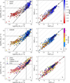 |
Fig. 9 Relationships between global and beam quantities, namely star formation efficiency, SFE, left column, and molecular gas fraction fmol, right column, colour-coded by the distance from the SFMS (ΔSFMS, top row), morphology (middle row), and the different samples included in the database (bottom row). In the panels, the black full line shows the 1:1 locus, while grey dotted lines are separated by 1 dex. The black dashed lines in the left column indicate a τdep = 2 Gyr. In the top row, the yellow pentagons show the positions of the wAGN-hosts in the sample, while the yellow stars show the positions of sAGN-hosts. In the middle row, dark blue dots show the locations of the SAB/SB galaxies. In the panels, the transparent diamonds are used to indicate that a given measurement is obtained with a CO upper limit. While fmol does not appear to vary across the galaxy discs, the SFE in the centre of the retired early-type galaxies in particular is ~1 dex lower compared to the SFE across the entire galaxies. |
Data availability
The full figure of Appendix B is available on Zenodo at https://zenodo.org/records/15387356. Table C.1 is available at the CDS via anonymous ftp to cdsarc.cds.unistra.fr (130.79.128.5) or via https://cdsarc.cds.unistra.fr/viz-bin/cat/J/A+A/699/A366
Acknowledgements
This paper is dedicated to the memory of Karl Menten, who made this work (and many others) possible with his baby-telescope, APEX. The authors thank the anonymous referee for the precious comments that significantly improved the paper’s quality. D.C. thanks Kathryn Kreckel for the useful discussions about metallicity estimators. D.C., Z.B., and F.B. gratefully acknowledge the Collaborative Research Center 1601 (SFB 1601 sub-project B3) funded by the Deutsche Forschungsgemeinschaft (DFG, German Research Foundation) – 500700252. D.C. and A.W. acknowledge support by the Deutsche Forschungsgemeinschaft, DFG project number SFB956-A3. S.F.S. thanks the PAPIIT-DGAPA AG100622 project and CONACYT grant CF19-39578. This work was supported by UNAM PASPA – DGAPA. E.R. acknowledges the support of the Natural Sciences and Engineering Research Council of Canada (NSERC), funding reference number RGPIN-2017-03987. A.D.B., T.W., L.B., S.V., and R.C.L. acknowledge support from the National Science Foundation (NSF) through the collaborative research award AST-1615960. K.D.F. acknowledges support from NSF grant AAG 23-07440. T.W. and Y.C. acknowledge support from the NSF through grant AST-1616199. J.B.B. acknowledges support from the grant IA-100420 (PAPIIT-DGAPA, UNAM). J.B-B acknowledges funding from the grant IA-101522 (DGAPA-PAPIIT, UNAM) and support from the DGAPA-PASPA 2025 fellowship (UNAM). V.V. acknowledges support from the ALMA-ANID Postdoctoral Fellowship under the award ASTRO21-0062. R.C.L. acknowledges partial support for this work from the NSF under award AST-2102625. This research made use of Astropy15, a community-developed core Python package for Astronomy (Astropy Collaboration 2013, 2018); matplotlib (Hunter 2007); and numpy and scipy (Virtanen et al. 2020). Support for CARMA construction was derived from the Gordon and Betty Moore Foundation, the Eileen and Kenneth Norris Foundation, the Caltech Associates, the states of California, Illinois, and Maryland, and the NSF. Funding for CARMA development and operations was supported by NSF and the CARMA partner universities. The authors acknowledge the usage of the HyperLeda database (http://leda.univ-lyon1.fr), the NASA/IPAC Extragalactic Database (http://ned.ipac.caltech.edu), and the NASA/IPAC Infrared Science Archive (https://irsa.ipac.caltech.edu/frontpage/).
Appendix A CO(1-0)-to-H2 conversion factor dependences on gas-phase metallicity and stellar mass surface density
In this work, we adopt a CO(1-0)-to-H2 conversion factor (αCO(1–0)) modelled following the prescription of Bolatto et al. (2013), which accounts for dependences on gas-phase metallicity and total mass surface density (here assumed to be equivalent to the stellar surface density). Among these parameters, gas-phase metallicity is supposed to play a dominant role, as αCO(1–0) exhibits an exponential dependence on it (see equation 13). We compute gas-phase metallicity on a spaxel-by-spaxel basis using the O3N2 method (Pettini & Pagel 2004), which is applicable only in regions where ionisation is driven by star formation. To extend the metallicity estimation to regions where ionisation is dominated by old stars or AGNs, we construct a radial metallicity map based on the mass-metallicity relation (MZR) from Sánchez et al. (2017).
Figure A.1 compares the αCO(1–0) values obtained from this combined metallicity map with those derived solely from emission-line metallicities. For a robust comparison, we consider only emission-line metallicity maps that contain at least 20% of the spaxels of the combined metallicity map. This analysis reveals that αCO(1–0) values inferred from the combined metallicity map can differ by up to a factor of 2 from those based solely on emission-line metallicities. The largest discrepancies arise typically in cases where the fraction of spaxels with detectable emission lines is small relative to the total number of spaxels in the combined map. The ratio tends to unity for galaxies where the number of spaxels within the emission line metallicity map becomes equivalent to the combined metallicity map. This is particularly true in the case of the beam αCO(1–0) measurements, as nebular emission lines are typically detected in the central regions of the galaxies. Nonetheless, the observed discrepancies remain within the typical uncertainty range associated with αCO(1–0) determinations (approximately 0.3 dex; Bolatto et al. 2013), indicating that the choice between combined and emission line-only metallicity maps does not introduce a significant systematic bias in the resulting molecular gas mass estimates.
To evaluate the relative dependence of αCO(1–0) on metallicity and stellar mass surface density, Fig. A.2 (upper row) presents the correlation of global and beam αCO(1–0) measurements with these two parameters, both derived from the same galactic regions. We find that both global and beam αCO(1–0) measurements exhibit a strong anticorrelation with gas-phase metallicity. However, while global αCO(1–0) remains largely insensitive to ![$\[\Sigma_{*}^{\mathrm{G}}\]$](/articles/aa/full_html/2025/07/aa53179-24/aa53179-24-eq34.png) , beam αCO(1–0) reaches systematically lower values due to a significant dependence on
, beam αCO(1–0) reaches systematically lower values due to a significant dependence on ![$\[\Sigma_{*}^{\mathrm{B}}\]$](/articles/aa/full_html/2025/07/aa53179-24/aa53179-24-eq35.png) .
.
The lower row of Fig.A.2, analogous to Fig.7, illustrates the distributions of global and beam gas-phase metallicity and stellar mass surface density. Here, beam stellar mass surface densities are calculated considering the beam stellar mass divided by the physical area defined by the APEX beam, while the global stellar mass surface densities are given by the global stellar mass divided by the physical area encompassed by 2 Re, which is the typical coverage of the galaxies by the CALIFA IFU. Beamevaluated metallicity measurements are systematically shifted towards higher values compared to their global counterparts, consistent with the lower beam αCO(1–0) values observed in Section 4.3.3. The distributions of Σ* measurements exhibit a similar trend; however, this appears to have a minimal impact on the final global αCO(1–0) values. These comparisons confirm that the adopted αCO(1–0) prescription is primarily governed by its dependence on gas-phase metallicity, while variations in stellar mass surface density, although affecting beam-scale estimates, do not significantly alter the resulting global values, thus validating the robustness of the chosen parametrisation.
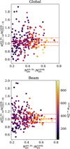 |
Fig. A.1 Ratio of the αCO(1–0) calculated from the gas-phase metallicity inferred only from nebular emission lines ( |
![$\[\alpha_{\mathrm{CO}(1-0)}^{\text {em.lin.}}\]$](/articles/aa/full_html/2025/07/aa53179-24/aa53179-24-eq36.png)
![$\[\alpha_{\mathrm{CO}(1-0)}^{\text {comb. }}\]$](/articles/aa/full_html/2025/07/aa53179-24/aa53179-24-eq37.png)
Appendix B Menagerie of galaxies and spectra in the iEDGE
In this section, we collected the discrete Hα flux maps of the galaxies together with the CO spectra observed by APEX, CARMA and/or ACA. In the following, Hα flux maps are shown in the first column of the figure, where the colour maps are based on the galaxy morphology: blue stretches for spirals, red stretches for elliptical, yellow stretches for lenticular, and grey stretches for irregular or galaxies with undefined morphology. CO spectra from APEX, CARMA, and ACA (if available) are shown in the right columns. In particular, CARMA D+E configuration data are shown in yellow, while CARMA E-only configuration data are in green. The full figure is available on Zenodo at https://zenodo.org/records/15387356.
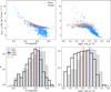 |
Fig. A.2 Upper row: Relation between beam (blue circles) and global (red dots) αCO(1–0) measurements on gas-phase metallicity (12+log(O/H), left panel) and stellar mass surface density (Σ* right panel) calculated within the same regions. Bottom row: Distributions of metallicity and stellar mass surface density. The histograms show median metallicity and integrated Σ* calculated across the full maps (global, empty black histograms) and tapered maps (beam, grey histograms). The red (blue) dashed lines indicate the median of the global (beam) quantities, while the green dash-dotted line (left panel) shows the solar metallicity (8.69 by Allende Prieto et al. 2001). |
Appendix C Content of the iEDGE current data release
Quantities included in the current data release of the iEDGE.
References
- Alatalo, K., Davis, T. A., Bureau, M., et al. 2013, MNRAS, 432, 1796 [NASA ADS] [CrossRef] [Google Scholar]
- Allende Prieto, C., Lambert, D. L., & Asplund, M. 2001, ApJ, 556, L63 [Google Scholar]
- Appleby, S., Davé, R., Sorini, D., Anglés-Alcázar, D., & Narayanan, D. 2020, MNRAS, 494, 6053 [NASA ADS] [CrossRef] [Google Scholar]
- Asplund, M., Grevesse, N., Sauval, A. J., & Scott, P. 2009, Ann. Rev. Astron. Astrophys., 47, 481 [CrossRef] [Google Scholar]
- Astropy Collaboration (Robitaille, T. P., et al.) 2013, A&A, 558, A33 [NASA ADS] [CrossRef] [EDP Sciences] [Google Scholar]
- Astropy Collaboration (Price-Whelan, A. M., et al.) 2018, AJ, 156, 123 [Google Scholar]
- Astropy Collaboration (Price-Whelan, A. M., et al.) 2022, ApJ, 935, 167 [NASA ADS] [CrossRef] [Google Scholar]
- Baker, W. M., Maiolino, R., Bluck, A. F. L., et al. 2022, MNRAS, 510, 3622 [NASA ADS] [CrossRef] [Google Scholar]
- Baldwin, J. A., Phillips, M. M., & Terlevich, R. 1981, PASP, 93, 5 [Google Scholar]
- Barrera-Ballesteros, J. K., García-Lorenzo, B., Falcón-Barroso, J., et al. 2015, A&A, 582, A21 [NASA ADS] [CrossRef] [EDP Sciences] [Google Scholar]
- Barrera-Ballesteros, J. K., Utomo, D., Bolatto, A. D., et al. 2020, MNRAS, 492, 2651 [NASA ADS] [CrossRef] [Google Scholar]
- Bigiel, F., Leroy, A. K., Walter, F., et al. 2011, ApJ, 730, L13 [NASA ADS] [CrossRef] [Google Scholar]
- Bluck, A. F. L., Mendel, J. T., Ellison, S. L., et al. 2014, MNRAS, 441, 599 [NASA ADS] [CrossRef] [Google Scholar]
- Bluck, A. F. L., Bottrell, C., Teimoorinia, H., et al. 2019, MNRAS, 485, 666 [Google Scholar]
- Bolatto, A. D., Wolfire, M., & Leroy, A. K. 2013, ARA&A, 51, 207 [CrossRef] [Google Scholar]
- Bolatto, A. D., Wong, T., Utomo, D., et al. 2017, ApJ, 846, 159 [Google Scholar]
- Boselli, A., Gavazzi, G., Lequeux, J., et al. 1997, A&A, 327, 522 [NASA ADS] [Google Scholar]
- Bothwell, M. S., Wagg, J., Cicone, C., et al. 2014, MNRAS, 445, 2599 [NASA ADS] [CrossRef] [Google Scholar]
- Braine, J., Combes, F., Casoli, F., et al. 1993, A&AS, 97, 887 [Google Scholar]
- Brinchmann, J., Charlot, S., White, S. D. M., et al. 2004, MNRAS, 351, 1151 [Google Scholar]
- Brownson, S., Belfiore, F., Maiolino, R., Lin, L., & Carniani, S. 2020, MNRAS, 498, L66 [NASA ADS] [CrossRef] [Google Scholar]
- Bundy, K., Bershady, M. A., Law, D. R., et al. 2015, ApJ, 798, 7 [Google Scholar]
- Cano-Díaz, M., Sánchez, S. F., Zibetti, S., et al. 2016, ApJ, 821, L26 [Google Scholar]
- Cappellari, M., Emsellem, E., Krajnović, D., et al. 2011, MNRAS, 413, 813 [Google Scholar]
- Cardelli, J. A., Clayton, G. C., & Mathis, J. S. 1989, ApJ, 345, 245 [Google Scholar]
- Catalán-Torrecilla, C., Gil de Paz, A., Castillo-Morales, A., et al. 2015, A&A, 584, A87 [NASA ADS] [CrossRef] [EDP Sciences] [Google Scholar]
- Chown, R., Li, C., Athanassoula, E., et al. 2019, MNRAS, 484, 5192 [NASA ADS] [CrossRef] [Google Scholar]
- Chown, R., Li, C., Parker, L., et al. 2021, MNRAS, 500, 1261 [Google Scholar]
- Cicone, C., Maiolino, R., Sturm, E., et al. 2014, A&A, 562, A21 [NASA ADS] [CrossRef] [EDP Sciences] [Google Scholar]
- Cicone, C., Bothwell, M., Wagg, J., et al. 2017, A&A, 604, A53 [NASA ADS] [CrossRef] [EDP Sciences] [Google Scholar]
- Cid Fernandes, R., Stasińska, G., Schlickmann, M. S., et al. 2010, MNRAS, 403, 1036 [Google Scholar]
- Cid Fernandes, R., Pérez, E., García Benito, R., et al. 2013, A&A, 557, A86 [NASA ADS] [CrossRef] [EDP Sciences] [Google Scholar]
- Colombo, D., Kalinova, V., Utomo, D., et al. 2018, MNRAS, 475, 1791 [NASA ADS] [CrossRef] [Google Scholar]
- Colombo, D., Rosolowsky, E., Duarte-Cabral, A., et al. 2019, MNRAS, 483, 4291 [NASA ADS] [CrossRef] [Google Scholar]
- Colombo, D., Sanchez, S. F., Bolatto, A. D., et al. 2020, A&A, 644, A97 [EDP Sciences] [Google Scholar]
- Combes, F., Young, L. M., & Bureau, M. 2007, MNRAS, 377, 1795 [NASA ADS] [CrossRef] [Google Scholar]
- Cook, R. H. W., Cortese, L., Catinella, B., & Robotham, A. 2020, MNRAS, 493, 5596 [NASA ADS] [CrossRef] [Google Scholar]
- Costa-Souza, J. H., Riffel, R. A., Souza-Oliveira, G. L., et al. 2024, ApJ, 974, 127 [Google Scholar]
- Daddi, E., Dickinson, M., Morrison, G., et al. 2007, ApJ, 670, 156 [NASA ADS] [CrossRef] [Google Scholar]
- Davis, T. A., Alatalo, K., Sarzi, M., et al. 2011, MNRAS, 417, 882 [Google Scholar]
- Davis, T. A., Alatalo, K., Bureau, M., et al. 2013, MNRAS, 429, 534 [Google Scholar]
- Davis, T. A., Young, L. M., Crocker, A. F., et al. 2014, MNRAS, 444, 3427 [NASA ADS] [CrossRef] [Google Scholar]
- Davis, T. A., Greene, J. E., Ma, C.-P., et al. 2019, MNRAS, 486, 1404 [NASA ADS] [CrossRef] [Google Scholar]
- den Brok, J. S., Chatzigiannakis, D., Bigiel, F., et al. 2021, MNRAS, 504, 3221 [NASA ADS] [CrossRef] [Google Scholar]
- den Brok, J. S., Leroy, A. K., Usero, A., et al. 2023, MNRAS, 526, 6347 [Google Scholar]
- Díaz-García, S., Lisenfeld, U., Pérez, I., et al. 2021, A&A, 654, A135 [NASA ADS] [CrossRef] [EDP Sciences] [Google Scholar]
- Domínguez-Gómez, J., Lisenfeld, U., Pérez, I., et al. 2022, A&A, 658, A124 [NASA ADS] [CrossRef] [EDP Sciences] [Google Scholar]
- Donnari, M., Pillepich, A., Joshi, G. D., et al. 2021, MNRAS, 500, 4004 [Google Scholar]
- Draine, B. T. 2011, Physics of the Interstellar and Intergalactic Medium (Princeton, NJ: Princeton University Press) [Google Scholar]
- Dubois, Y., Gavazzi, R., Peirani, S., & Silk, J. 2013, MNRAS, 433, 3297 [CrossRef] [Google Scholar]
- Ellison, S. L., Sánchez, S. F., Ibarra-Medel, H., et al. 2018, MNRAS, 474, 2039 [Google Scholar]
- Ellison, S. L., Thorp, M. D., Lin, L., et al. 2020, MNRAS, 493, L39 [CrossRef] [Google Scholar]
- Ellison, S. L., Lin, L., Thorp, M. D., et al. 2021a, MNRAS, 502, L6 [Google Scholar]
- Ellison, S. L., Lin, L., Thorp, M. D., et al. 2021b, MNRAS, 501, 4777 [Google Scholar]
- Ellison, S. L., Wong, T., Sánchez, S. F., et al. 2021c, MNRAS, 505, L46 [Google Scholar]
- Ellison, S. L., Pan, H.-A., Bluck, A. F. L., et al. 2024, MNRAS, 527, 10201 [Google Scholar]
- Flewelling, H. A., Magnier, E. A., Chambers, K. C., et al. 2020, ApJS, 251, 7 [NASA ADS] [CrossRef] [Google Scholar]
- Gao, Y., Xiao, T., Li, C., et al. 2019, ApJ, 887, 172 [Google Scholar]
- García-Benito, R., Zibetti, S., Sánchez, S. F., et al. 2015, A&A, 576, A135 [Google Scholar]
- Genzel, R., Tacconi, L. J., Lutz, D., et al. 2015, ApJ, 800, 20 [Google Scholar]
- González Delgado, R. M., Cid Fernandes, R., Pérez, E., et al. 2016, A&A, 590, A44 [NASA ADS] [CrossRef] [EDP Sciences] [Google Scholar]
- Güsten, R., Nyman, L. Å., Schilke, P., et al. 2006, A&A, 454, L13 [NASA ADS] [CrossRef] [EDP Sciences] [Google Scholar]
- Hogarth, L. M., Saintonge, A., Davis, T. A., et al. 2024, MNRAS, 528, 6768 [Google Scholar]
- Hunter, J. D. 2007, Comput. Sci. Eng., 9, 90 [NASA ADS] [CrossRef] [Google Scholar]
- Kalinova, V., Colombo, D., Sánchez, S. F., et al. 2021, A&A, 648, A64 [NASA ADS] [CrossRef] [EDP Sciences] [Google Scholar]
- Kalinova, V., Colombo, D., Sánchez, S. F., et al. 2022, A&A, 665, A90 [NASA ADS] [CrossRef] [EDP Sciences] [Google Scholar]
- Keenan, R. P., Marrone, D. P., Keating, G. K., et al. 2024, ApJ, 975, 150 [Google Scholar]
- Kelly, B. C. 2007, ApJ, 665, 1489 [Google Scholar]
- Kenney, J. D., & Young, J. S. 1988, ApJS, 66, 261 [NASA ADS] [CrossRef] [Google Scholar]
- Kennicutt, Jr., R. C. 1998, ApJ, 498, 541 [Google Scholar]
- Kewley, L. J., Dopita, M. A., Sutherland, R. S., Heisler, C. A., & Trevena, J. 2001, ApJ, 556, 121 [Google Scholar]
- Koss, M. J., Strittmatter, B., Lamperti, I., et al. 2021, ApJS, 252, 29 [CrossRef] [Google Scholar]
- Lacerda, E. A. D., Cid Fernandes, R., Couto, G. S., et al. 2018, MNRAS, 474, 3727 [Google Scholar]
- Lacerda, E. A. D., Sánchez, S. F., Cid Fernandes, R., et al. 2020, MNRAS, 492, 3073 [Google Scholar]
- Lees, J. F., Knapp, G. R., Rupen, M. P., & Phillips, T. G. 1991, ApJ, 379, 177 [Google Scholar]
- Leroy, A. K., Bolatto, A., Gordon, K., et al. 2011, ApJ, 737, 12 [Google Scholar]
- Leroy, A. K., Walter, F., Sandstrom, K., et al. 2013, AJ, 146, 19 [Google Scholar]
- Leroy, A. K., Sandstrom, K. M., Lang, D., et al. 2019, ApJS, 244, 24 [Google Scholar]
- Leroy, A. K., Schinnerer, E., Hughes, A., et al. 2021, ApJS, 257, 43 [NASA ADS] [CrossRef] [Google Scholar]
- Leroy, A. K., Rosolowsky, E., Usero, A., et al. 2022, ApJ, 927, 149 [NASA ADS] [CrossRef] [Google Scholar]
- Lin, L., Pan, H.-A., Ellison, S. L., et al. 2019, ApJ, 884, L33 [NASA ADS] [CrossRef] [Google Scholar]
- Lin, L.-H., Wang, H.-C., Su, Y., Li, C., & Yang, J. 2020, Res. Astron. Astrophys., 20, 143 [CrossRef] [Google Scholar]
- Lin, L., Ellison, S. L., Pan, H.-A., et al. 2022, ApJ, 926, 175 [Google Scholar]
- Lodders, K. 2003, ApJ, 591, 1220 [Google Scholar]
- McKee, C. F., & Ostriker, E. C. 2007, ARA&A, 45, 565 [Google Scholar]
- Michałowski, M. J., Gall, C., Hjorth, J., et al. 2024, ApJ, 964, 129 [CrossRef] [Google Scholar]
- Narayanan, D., & Krumholz, M. R. 2014, MNRAS, 442, 1411 [NASA ADS] [CrossRef] [Google Scholar]
- Ni, Y., Chen, N., Zhou, Y., et al. 2024, arXiv e-prints [arXiv:2409.10666] [Google Scholar]
- Pan, H.-A., Lin, L., Ellison, S. L., et al. 2024, ApJ, 964, 120 [Google Scholar]
- Pettini, M., & Pagel, B. E. J. 2004, MNRAS, 348, L59 [NASA ADS] [CrossRef] [Google Scholar]
- Piotrowska, J. M., Bluck, A. F. L., Maiolino, R., Concas, A., & Peng, Y. 2020, MNRAS, 492, L6 [Google Scholar]
- Piotrowska, J. M., Bluck, A. F. L., Maiolino, R., & Peng, Y. 2022, MNRAS, 512, 1052 [NASA ADS] [CrossRef] [Google Scholar]
- Rahman, N., Bolatto, A. D., Xue, R., et al. 2012, ApJ, 745, 183 [NASA ADS] [CrossRef] [Google Scholar]
- Renzini, A., & Peng, Y.-j. 2015, ApJ, 801, L29 [NASA ADS] [CrossRef] [Google Scholar]
- Rodríguez, M. I., Lisenfeld, U., Duarte Puertas, S., et al. 2024, A&A, 692, A125 [NASA ADS] [CrossRef] [EDP Sciences] [Google Scholar]
- Rosario, D. J., Burtscher, L., Davies, R. I., et al. 2018, MNRAS, 473, 5658 [NASA ADS] [CrossRef] [Google Scholar]
- Rosolowsky, E., Hughes, A., Leroy, A. K., et al. 2021, MNRAS, 502, 1218 [NASA ADS] [CrossRef] [Google Scholar]
- Sage, L. J. 1993, A&AS, 100, 537 [NASA ADS] [Google Scholar]
- Saintonge, A., & Catinella, B. 2022, ARA&A, 60, 319 [NASA ADS] [CrossRef] [Google Scholar]
- Saintonge, A., Kauffmann, G., Wang, J., et al. 2011, MNRAS, 415, 61 [NASA ADS] [CrossRef] [Google Scholar]
- Saintonge, A., Catinella, B., Cortese, L., et al. 2016, MNRAS, 462, 1749 [Google Scholar]
- Saintonge, A., Catinella, B., Tacconi, L. J., et al. 2017, ApJS, 233, 22 [Google Scholar]
- Saintonge, A., Wilson, C. D., Xiao, T., et al. 2018, MNRAS, 481, 3497 [NASA ADS] [CrossRef] [Google Scholar]
- Salim, S., Rich, R. M., Charlot, S., et al. 2007, ApJS, 173, 267 [NASA ADS] [CrossRef] [Google Scholar]
- Salpeter, E. E. 1955, ApJ, 121, 161 [Google Scholar]
- Sánchez, S. F. 2020, ARA&A, 58, 99 [Google Scholar]
- Sánchez, S. F., Kennicutt, R. C., Gil de Paz, A., et al. 2012, A&A, 538, A8 [Google Scholar]
- Sánchez, S. F., Rosales-Ortega, F. F., Iglesias-Páramo, J., et al. 2014, A&A, 563, A49 [CrossRef] [EDP Sciences] [Google Scholar]
- Sánchez, S. F., García-Benito, R., Zibetti, S., et al. 2016a, A&A, 594, A36 [NASA ADS] [CrossRef] [EDP Sciences] [Google Scholar]
- Sánchez, S. F., Pérez, E., Sánchez-Blázquez, P., et al. 2016b, Rev. Mexicana Astron. Astrofis., 52, 171 [Google Scholar]
- Sánchez, S. F., Pérez, E., Sánchez-Blázquez, P., et al. 2016c, Rev. Mexicana Astron. Astrofis., 52, 21 [Google Scholar]
- Sánchez, S. F., Barrera-Ballesteros, J. K., Sánchez-Menguiano, L., et al. 2017, MNRAS, 469, 2121 [CrossRef] [Google Scholar]
- Sánchez, S. F., Avila-Reese, V., Hernandez-Toledo, H., et al. 2018, Rev. Mexicana Astron. Astrofis., 54, 217 [Google Scholar]
- Sánchez, S. F., Barrera-Ballesteros, J. K., Colombo, D., et al. 2021, MNRAS, 503, 1615 [CrossRef] [Google Scholar]
- Sánchez, S. F., Galbany, L., Walcher, C. J., García-Benito, R., & BarreraBallesteros, J. K. 2023, MNRAS, 526, 5555 [CrossRef] [Google Scholar]
- Sanders, D. B., & Mirabel, I. F. 1985, ApJ, 298, L31 [Google Scholar]
- Sandstrom, K. M., Leroy, A. K., Walter, F., et al. 2013, ApJ, 777, 5 [Google Scholar]
- Scaloni, L., Rodighiero, G., Enia, A., et al. 2024, A&A, 687, A255 [NASA ADS] [CrossRef] [EDP Sciences] [Google Scholar]
- Solomon, P. M., Downes, D., Radford, S. J. E., & Barrett, J. W. 1997, ApJ, 478, 144 [NASA ADS] [CrossRef] [Google Scholar]
- Sun, J., Leroy, A. K., Schruba, A., et al. 2018, ApJ, 860, 172 [NASA ADS] [CrossRef] [Google Scholar]
- Sun, J., Leroy, A. K., Schinnerer, E., et al. 2020, ApJ, 901, L8 [NASA ADS] [CrossRef] [Google Scholar]
- Sun, J., Leroy, A. K., Ostriker, E. C., et al. 2023, ApJ, 945, L19 [NASA ADS] [CrossRef] [Google Scholar]
- Tacconi, L. J., Genzel, R., Neri, R., et al. 2010, Nature, 463, 781 [Google Scholar]
- Tacconi, L. J., Neri, R., Genzel, R., et al. 2013, ApJ, 768, 74 [NASA ADS] [CrossRef] [Google Scholar]
- Tacconi, L. J., Genzel, R., Saintonge, A., et al. 2018, ApJ, 853, 179 [Google Scholar]
- Thorp, M. D., Ellison, S. L., Pan, H.-A., et al. 2022, MNRAS, 516, 1462 [NASA ADS] [CrossRef] [Google Scholar]
- Thronson, Harley A., J., Tacconi, L., Kenney, J., et al. 1989, ApJ, 344, 747 [NASA ADS] [CrossRef] [Google Scholar]
- Utomo, D., Bolatto, A. D., Wong, T., et al. 2017, ApJ, 849, 26 [NASA ADS] [CrossRef] [Google Scholar]
- Verter, F. 1985, ApJS, 57, 261 [Google Scholar]
- Villanueva, V., Bolatto, A., Vogel, S., et al. 2021, ApJ, 923, 60 [Google Scholar]
- Villanueva, V., Bolatto, A. D., Vogel, S. N., et al. 2024, ApJ, 962, 88 [NASA ADS] [CrossRef] [Google Scholar]
- Virtanen, P., Gommers, R., Oliphant, T. E., et al. 2020, Nat. Methods, 17, 261 [Google Scholar]
- Walcher, C. J., Wisotzki, L., Bekeraité, S., et al. 2014, A&A, 569, A1 [NASA ADS] [CrossRef] [EDP Sciences] [Google Scholar]
- Wang, Z., Kenney, J. D. P., & Ishizuki, S. 1992, AJ, 104, 2097 [Google Scholar]
- Welch, G. A., Sage, L. J., & Young, L. M. 2010, ApJ, 725, 100 [NASA ADS] [CrossRef] [Google Scholar]
- Wiklind, T., & Henkel, C. 1989, A&A, 225, 1 [NASA ADS] [Google Scholar]
- Wiklind, T., Combes, F., & Henkel, C. 1995, A&A, 297, 643 [NASA ADS] [Google Scholar]
- Wilson, R. W., Jefferts, K. B., & Penzias, A. A. 1970, ApJ, 161, L43 [NASA ADS] [CrossRef] [Google Scholar]
- Wong, T., Cao, Y., Luo, Y., et al. 2024, ApJS, 271, 35 [Google Scholar]
- Wylezalek, D., Cicone, C., Belfiore, F., et al. 2022, MNRAS, 510, 3119 [CrossRef] [Google Scholar]
- Yajima, Y., Sorai, K., Miyamoto, Y., et al. 2021, PASJ, 73, 257 [NASA ADS] [CrossRef] [Google Scholar]
- York, D. G., Adelman, J., Anderson, Jr., J. E., et al. 2000, AJ, 120, 1579 [NASA ADS] [CrossRef] [Google Scholar]
- Young, J. S., Xie, S., Tacconi, L., et al. 1995, ApJS, 98, 219 [NASA ADS] [CrossRef] [Google Scholar]
- Young, L. M., Bureau, M., Davis, T. A., et al. 2011, MNRAS, 414, 940 [NASA ADS] [CrossRef] [Google Scholar]
- Yu, S.-Y., Kalinova, V., Colombo, D., et al. 2022, A&A, 666, A175 [NASA ADS] [CrossRef] [EDP Sciences] [Google Scholar]
- Yuan, F., Yoon, D., Li, Y.-P., et al. 2018, ApJ, 857, 121 [Google Scholar]
The current data release of the PYTHON-based EDGE is available at https://github.com/tonywong94/edge_pydb
Using ASTROPY GAUSSIAN2D function, see https://docs.astropy.org/en/stable/api/astropy.modeling.functional_models.Gaussian2D.html
CO Legacy Database for GASS, Saintonge et al. (2011).
All Tables
All Figures
|
Fig. 1 Aperture correction for APEX observation-related tests and measurements. Upper left: global versus beam luminosities calculated for WISE W3 (12 μm; green), ACA (red), and CARMA (blue) detected galaxies. The dotted lines indicate the 2:1, 5:1, and 10:1 loci, respectively. Upper middle: CO(2-1) luminosities from APEX measurements |
| In the text | |
|
Fig. 2 Number of galaxies within the iEDGE observed by the different telescopes represented as a Venn diagram. Objects solely observed by APEX eventually constitute 64% of the final database, and CARMA data add up to 22% of the database. The rest of the targets have been observed by multiple telescopes. |
| In the text | |
|
Fig. 3 Comparison between beam-wise (top panels) and global luminosities (bottom panels) from ACA and APEX (left panels) and from CARMA and APEX (right panels). The blue circles indicate galaxies detected (with S/N > 3) from both telescopes, yellow arrows indicate galaxies detected only by ACA or CARMA, the green arrows indicate galaxies detected only by APEX, and the red crosses show galaxies not detected by both telescopes. For non-detections, luminosities are given as upper limits. For global luminosities, we show only the detections from both telescopes (see the text for further details). The black solid lines mark the 1:1 locus. The magenta dashed line has a unitary slope and an intercept equal to the median ratio between the x – and the y-quantities. In addition, in the left panels, the dotted black line marks the location where the CO(2-1)-to-CO(1-0) ratio, R21 = 0.65. The grey dashed lines have a unitary slope and are separated by 0.5 dex. |
| In the text | |
|
Fig. 4 Detection distance bias shown as the beam S/N vs the distance to the galaxies, for APEX- (red), CARMA- (yellow), CARMA (D+E)- (green empty), ACA- (blue) observed galaxies. The black dashed line indicates a S/N=3 that marks the separation between detections and nondetections. Non-detections (observations with S/N<3) starkly decrease from a distance >130 Mpc and are all related to APEX observations. |
| In the text | |
|
Fig. 5 SFR-M* diagrams defined by the different samples considered in this paper (left panel): full CALIFA (cyan hexagons), and galaxies observed in CO lines by APEX (red circles), CARMA (yellow diamonds), CARMA (D+E galaxies only, empty green diamonds), ACA (blue squares). In the right panel, the red circles represent CO-detected galaxies (with S/N > 3), while the black dots show CO non-detections (with S/N < 3). In both panels, the black line shows Cano-Díaz et al. (2016) the SFMS model with the uncertainties (dotted lines). The dashed purple line indicates the green valley boundary position defined in C20, which is located 3σ (equal to 0.20 dex as in Cano-Díaz et al. 2016) from the SFMS. APEX targets extend from the SFMS to the retired regions, better representing the CALIFA galaxies in this diagram. |
| In the text | |
|
Fig. 6 Histograms across samples (full CALIFA, cyan bars; galaxies in the full iEDGE sample, black empty bars; CO detected galaxies in the iEDGE, red bars) related (from left to right) to M*, SFR, specific SFR (sSFR=SFR/M*), and logarithmic distance from the SF main sequence (ΔSFMS). Similarly to CALIFA, iEDGE spans a representative range of SFR, M*, and related values. However, CO detections decrease at low sSFR and ΔSFMS values. |
| In the text | |
|
Fig. 7 Distributions of the inferred CO(2-1)-to-CO(1-0) ratio (R21, left) and CO(1-0)-to-H2 conversion factors (αCO(1–0), right). These quantities are derived using IFU maps from models described in Equations (13) and (14) (for αCO(1–0) and R21, respectively). Histograms show median R21 and αCO(1–0) calculated across the full maps (global, empty black histograms) and tapered maps (beam, grey histograms). The red (blue) dashed lines indicate the median of the global (beam) quantities, while the green dash-dotted lines show the typical values adopted for star-forming galaxies in the local Universe (e.g. R21 = 0.65 and αCO(1–0) = 4.35 M⊙ (pc2 K km s−1)−1). Regarding R21, we measured medians (depending on the coverage) generally lower than the average values observed in nearby galaxies. The αCO(1–0) values span an order of magnitude, with lower conversion factors measured within the galaxy centres. This is consistent with the fact that galaxies exhibit a declining metallicity trend with respect to the galactocentric radius, hence showing lower αCO(1–0) in their centre (see also Appendix A). |
| In the text | |
|
Fig. 8 Star formation scaling relations studied here colour-coded by the median equivalent width of Hα (WHα, upper row) and morphology (lower row), from left to right SFR-M*, SFR-Mmol, and Mmol − M*. In the left panel, the elements follow Fig. 5; additionally, the dotted lines are spaced of 3σ from each other. In the middle panel, the black solid line indicates a constant molecular depletion time τdep = 2 Gyr, additionally, dotted lines show constant τdep from (top to bottom) 10−5 to 107 Gyr. In the right panel, the black line indicates a constant molecular gas-to-stellar mass fmol = 0.1; additionally, the dotted lines show constant fmol from (bottom to top) 10−5 to 104. The triangles in the middle and right panels illustrate galaxies for which upper limits for the molecular gas mass are used. At the bottom right of each panel the typical (median) uncertainty for the quantities is shown. In the upper row, the pentagons show the positions of the wAGN-hosts in the sample, while the stars show the positions of sAGN-hosts. In the lower row, the dark blue dots show the locations of the SAB/SB galaxies. Spiral star-forming galaxies on the one hand and early-type retired galaxies on the other hand describe well-defined relationships across the three diagrams. |
| In the text | |
|
Fig. 9 Relationships between global and beam quantities, namely star formation efficiency, SFE, left column, and molecular gas fraction fmol, right column, colour-coded by the distance from the SFMS (ΔSFMS, top row), morphology (middle row), and the different samples included in the database (bottom row). In the panels, the black full line shows the 1:1 locus, while grey dotted lines are separated by 1 dex. The black dashed lines in the left column indicate a τdep = 2 Gyr. In the top row, the yellow pentagons show the positions of the wAGN-hosts in the sample, while the yellow stars show the positions of sAGN-hosts. In the middle row, dark blue dots show the locations of the SAB/SB galaxies. In the panels, the transparent diamonds are used to indicate that a given measurement is obtained with a CO upper limit. While fmol does not appear to vary across the galaxy discs, the SFE in the centre of the retired early-type galaxies in particular is ~1 dex lower compared to the SFE across the entire galaxies. |
| In the text | |
|
Fig. A.1 Ratio of the αCO(1–0) calculated from the gas-phase metallicity inferred only from nebular emission lines ( |
| In the text | |
|
Fig. A.2 Upper row: Relation between beam (blue circles) and global (red dots) αCO(1–0) measurements on gas-phase metallicity (12+log(O/H), left panel) and stellar mass surface density (Σ* right panel) calculated within the same regions. Bottom row: Distributions of metallicity and stellar mass surface density. The histograms show median metallicity and integrated Σ* calculated across the full maps (global, empty black histograms) and tapered maps (beam, grey histograms). The red (blue) dashed lines indicate the median of the global (beam) quantities, while the green dash-dotted line (left panel) shows the solar metallicity (8.69 by Allende Prieto et al. 2001). |
| In the text | |
Current usage metrics show cumulative count of Article Views (full-text article views including HTML views, PDF and ePub downloads, according to the available data) and Abstracts Views on Vision4Press platform.
Data correspond to usage on the plateform after 2015. The current usage metrics is available 48-96 hours after online publication and is updated daily on week days.
Initial download of the metrics may take a while.