| Issue |
A&A
Volume 644, December 2020
|
|
|---|---|---|
| Article Number | A97 | |
| Number of page(s) | 12 | |
| Section | Interstellar and circumstellar matter | |
| DOI | https://doi.org/10.1051/0004-6361/202039005 | |
| Published online | 04 December 2020 | |
The EDGE-CALIFA survey: exploring the role of molecular gas on galaxy star formation quenching
1
Max-Planck-Institut für Radioastronomie,
Auf dem Hügel 69,
53121
Bonn, Germany
e-mail: This email address is being protected from spambots. You need JavaScript enabled to view it.
2
Instituto de Astronomiá, Universidad Nacional Autonóma de Mexico,
A.P. 70-264,
04510
México,
D.F., Mexico
3
Department of Astronomy, University of Maryland,
College Park,
MD
20742, USA
4
Department of Astronomy, University of Illinois,
Urbana,
IL
61801, USA
5
Department of Physics, University of Alberta,
4-181 CCIS,
Edmonton,
AB
T6G 2E1, Canada
6
Instituto de Astrofísica de Canarias,
38205
La Laguna,
Tenerife, Spain
7
Universidad de La Laguna, Departamento de Astrofísica,
38206
La Laguna,
Tenerife, Spain
8
Aix-Marseille Univ, CNRS, CNES, LAM (Laboratoire d’Astrophysique de Marseille),
Marseille, France
9
Department of Astronomy, The Ohio State University,
140 West 18th Avenue,
Columbus,
OH
43210, USA
10
Department of Astronomy, University of California,
Berkeley,
CA
94720, USA
Received:
23
July
2020
Accepted:
16
September
2020
Abstract
Understanding how galaxies cease to form stars represents an outstanding challenge for galaxy evolution theories. This process of “star formation quenching” has been related to various causes, including active galactic nuclei activity, the influence of large-scale dynamics, and the environment in which galaxies live. In this paper, we present the first results from a follow-up of CALIFA survey galaxies with observations of molecular gas obtained with the APEX telescope. Together with the EDGE-CARMA observations, we collected 12CO observations that cover approximately one effective radius in 472 CALIFA galaxies. We observe that the deficit of galaxy star formation with respect to the star formation main sequence (SFMS) increases with the absence of molecular gas and with a reduced efficiency of conversion of molecular gas into stars, which is in line with the results of other integrated studies. However, by dividing the sample into galaxies dominated by star formation and galaxies quenched in their centres (as indicated by the average value of the Hα equivalent width), we find that this deficit increases sharply once a certain level of gas consumption is reached, indicating that different mechanisms drive separation from the SFMS in star-forming and quenched galaxies. Our results indicate that differences in the amount of molecular gas at a fixed stellar mass are the primary drivers for the dispersion in the SFMS, and the most likely explanation for the start of star formation quenching. However, once a galaxy is quenched, changes in star formation efficiency drive how much a retired galaxy differs in its star formation rate from star-forming ones of similar masses. In other words, once a paucity of molecular gas has significantly reduced star formation, changes in the star formation efficiency are what drives a galaxy deeper into the red cloud, hence retiring it.
Key words: surveys / galaxies: ISM / ISM: molecules / evolution / galaxies: evolution / galaxies: star formation
© D. Colombo et al. 2020
 Open Access article, published by EDP Sciences, under the terms of the Creative Commons Attribution License (https://creativecommons.org/licenses/by/4.0), which permits unrestricted use, distribution, and reproduction in any medium, provided the original work is properly cited.
Open Access funding provided by Max Planck Society.
1 Introduction
The appearance of galaxies in the nearby Universe is largely shaped by their star formation activity. The cessation of star formation that accompanies the transformation of a blue, spiral galaxy into a “red-and-dead” elliptical is usually called star formation quenching (e.g. Faber et al. 2007). Quenching is generally associated with the shortage of the raw fuel that feeds the star formation: the cold gas, and in particular its molecular phase. In low-mass galaxies, the gas, which is weakly bound due to their shallow potential wells, can be promptly removed by stellar feedback (e.g. Dekel & Silk 1986). High-mass galaxies, instead, might require a more powerful way to disperse the gas, such as active galactic nuclei (AGN) outflows (e.g. Lacerda et al. 2020). By heating up the gas, AGN activity can also block the accretion from the intergalactic medium causing “quenching by starvation” (e.g. Cicone et al. 2014). Likewise, the suppression of cold gas accretion can result from shock heating in dark matter halos with masses >1012 M⊙ (“halo quenching”; e.g. Dekel & Birnboim 2006). Small galaxies falling towards a galaxy cluster can have their gas removed by tidal stripping (e.g. Abadi et al. 1999), or through the interaction with a hot intra-cluster medium (e.g. Moore et al. 1996) that prevents further accretion from the intergalactic medium (environmental quenching). Alternatively, galaxies can stop forming stars efficiently even if a substantial amount of gas is present. In this “morphological quenching” scenario, the development of a bulge or a spheroid, together with dispersive forces such as shear, stabilises the galactic gaseous disc against collapse, preventing star formation (Martig et al. 2009). Fully disentangling the dominant quenching mechanisms, their timescales, and their parameter dependence requires the analysis of cold gas conditions for a statistically significant sample of galaxies.
Major nearby galaxy cold gas mapping surveys (Regan et al. 2001; Wilson et al. 2009; Rahman et al. 2011; Leroy et al. 2009; Donovan Meyer et al. 2013; Bolatto et al. 2017; Sorai et al. 2019; Sun et al. 2018) have focused on observations of the molecular gas (through CO lines). Despite a few notable exceptions (e.g. Alatalo et al. 2013; Saintonge et al. 2017), these surveys observed mainly spiral or infrared-bright galaxies (i.e. galaxies with significant star formation) and have furthered our understanding of how star formation happens, rather than how it stops. This boils down to quantifying the relation between molecular gas and star formation rate (SFR), which appears nearly linear in nearby discs (Kennicutt 1998; Bigiel et al. 2008; Leroy et al. 2013; Lin et al. 2019). This relationship is often parametrised via the ratio between the SFR and the molecular gas mass (Mmol), which is called the molecular star formation efficiency (SFE = SFR/Mmol = 1∕τdep), where the inverse of the SFE is the depletion time, τdep. The depletion time indicates how much time is necessary to convert all the available molecular gas into stars at the current star formation rate. On kpc scales and in the discs of nearby star-forming galaxies, τdep is approximately constant around 1–2 Gyr (Bigiel et al. 2011; Rahman et al. 2012; Leroy et al. 2013; Utomo et al. 2017), and it appears to weakly correlate with many galactic properties such as stellar mass surface density or environmental hydrostatic pressure (Leroy et al. 2008; Rahman et al. 2012). Nevertheless, small but important deviations for a constant SFE have been noticed, which can be the first hints of star formation quenching. In some galaxies, the depletion time in the centres appear shorter (Leroy et al. 2013; Utomo et al. 2017) or longer (Utomo et al. 2017) with respectto their discs. These differences may correlate with the presence of a bar or with galaxy mergers (Utomo et al. 2017; see also Muraoka et al. 2019) and do not seem to be related to unaccounted variation in the CO-to-H2 conversion factor (Leroy et al. 2013; Utomo et al. 2017). Spiral arm streaming motions have also been observed to lengthen depletion times (Meidt et al. 2013; Leroy et al. 2015).
Besides variation of the SFE within galaxies, differences in global SFE between galaxies have been explored more widely in the nearby Universe, thanks especially to molecular gas galaxy-integrated studies (see Saintonge et al. 2011, 2017, and references therein). Those studies are less expensive in terms of exposure time compared to resolved mapping studies and provide the opportunity to collect data for larger galactic samples. In particular, integrated samples provide access to the molecular gas content of galaxies below the star formation main sequence (SFMS or MS, i.e. the locus of the star-forminggalaxies in the SFR stellar mass diagram, e.g. Brinchmann et al. 2004; Whitaker et al. 2012; Renzini & Peng 2015; Cano-Díaz et al. 2016), that is, galaxies that are slowly shutting down their star formation (located in the so-called green valley; Salim et al. 2007), down to passive galaxies (or “red sequence” galaxies, as defined on a colour-magnitude diagram). In general, galaxies on the main sequence have longer depletion times than similar stellar mass galaxies located below the main sequence (Saintonge et al. 2016, 2017). The reasons for this are unclear and might be due to a combination of effects. Barred and interacting galaxies generally show shorter global depletion times compared to other systems (Saintonge et al. 2012). Early-type galaxies show lower SFE compared to late-type objects (Davis et al. 2014) and some of the lowest values of SFE are observed in bulge-dominated galaxies (Saintonge et al. 2012). As star formation quenching is more often seen to happen inside-out (e.g. González Delgado et al. 2016), galaxy morphology and structural properties seem to play a role in modifying the SFE. On average, τdep,mol appears to decrease moving from early- to late-type systems (Colombo et al. 2018), following the decrease in shear (Davis et al. 2014; Colombo et al. 2018) as described by the morphological quenching scenario (however, see Koyama et al. 2019). The molecular depletion time is also seen to decrease with stellar surface densityand increase with molecular gas velocity dispersion (Dey et al. 2019). This might indicate that τdep,mol is longer for bulged systems, and where gas is less gravitationally bound (as the gas boundness is proportional to Σmol ∕σCO, i.e. the ratio between the molecular gas mass surface density and the CO velocity dispersion; see Leroy et al. 2015). The environment in which a galaxy lives might also be important: galaxies in clusters appear to have longer depletion times than group galaxies (e.g. Mok et al. 2016), possibly due to the turbulent pressure and additional heating induced by the cluster itself.
Nevertheless, most theories attribute star formation quenching to the absence of molecular gas, rather than to a less efficient conversion from gas to stars. This has been explored observationally mostly by integrated surveys (Genzel et al. 2015; Saintonge et al. 2016; Tacconi et al. 2018; Lin et al. 2017), which usually parameterised the shortage of gas through the molecular gas fraction, fmol = Mmol∕M*. This quantity seems to drop drastically for galaxies with M* > 1010.5−11 M⊙ (Saintonge et al. 2017; Bolatto et al. 2017) and for redder objects (Saintonge et al. 2011). It also appears reduced in barred galaxies (Bolatto et al. 2017). This absence appears tentatively connected to the presence of an AGN in a galaxy (Saintonge et al. 2017); negative feedback due to the AGN may provide an efficient gas-removal mechanism, which is suggested by the fact that AGN-hosting galaxies are almost exclusively observed in the green valley (see Lacerda et al. 2020). Nevertheless, this is still a matter of debate (e.g. Kirkpatrick et al. 2014; Rosario et al. 2018).
Despite several studies exploring the methods for quenching, there is not a clear conclusion as to whether the quenching is driven by the reduction in molecular gas content, a change in the star formation efficiency of the molecular gas, or both effects. Furthermore, these studies have not assessed how these effects may change throughout the quenching process. To address these shortcomings, in this work, rather than examining causes for SFE and fmol variations, we used the 12CO(1–0) maps from the Extragalactic Database for Galaxy Evolution (EDGE) survey (Bolatto et al. 2017) in combination with new 12CO(2–1) single-dish measurements to investigate whether SFE or fmol changes are the main cause of star formation quenching in the centre of more than 470 Calar Alto Legacy Integral Field Area (CALIFA) survey (Sánchez et al. 2016a) galaxies at different quenching stages. The paper is structured as follows: Sect. 2 exposes the data used in this paper, while Sect. 3 describes the quantities derived from these data such as SFRs and molecular gas masses (Mmol). The results of the analyses are shown in Sect. 4. Those results are discussed and summarised in Sect. 5. For the derived quantities, we assume here a cosmology H0 = 71 km s−1 Mpc−1, Ωm = 0.27, ΩΛ = 0.73.
2 Sample and data
We collected a homogenised compilation of 472 galaxies with molecular gas measured in an aperture of diameter 26.3″, which corresponds to the Atacama Pathfinder Experiment (APEX) beam at 230 GHz. This compilation comprises our new observationsusing APEX together with a re-analysis of Combined Array for Research in Millimeter-wave Astronomy (CARMA) observationsacquired by the EDGE collaboration (Bolatto et al. 2017). All galaxies were already covered by spatially resolved observations by the CALIFA survey (Sánchez et al. 2012). The sample of 472 galaxies covers a wide range of galaxy parameters in terms of morphology (from E to Sm, including a few irregular galaxies), stellar masses (107.2−1011.9 M⊙), and SFRs (10−4.0−101.3 M⊙ yr−1). Thus, it is one of the first explorations of a large sample not systematically biased by selection. The CARMA sample is generally made up of galaxies concentrated along the SFMS (as it has been assembled considering 22 μm bright WISE galaxies), while the APEX sample targets more uniformly cover the so-called green valley and red sequence, as we can see in Fig. 1. Together, the CARMA and APEX samples provide good coverage of the full extended CALIFA sample. The APEX and CARMA samples do not overlap, meaning that objects observed by CARMA in 12CO(1–0) have not been re-observed with APEX in 12CO(2–1).
An example of the quality of the APEX data and the rich variety of the targets in our dataset is given in Fig. 2. Spectra of APEX 12CO(2–1) observationsare illustrated in the first row. The centres of all the galaxies in this example are well detected in CO, but the continuum and Hα equivalent width (WHα) maps show that the objects are in three different phases of their evolution. On the left middle panel, the continuum map indicates that the galaxy (NGC 0873) is entirely blue, therefore dominated by star formation. Along with colour, WH α is also a faithful proxy for the star formation properties of the galaxies (e.g. Sánchez 2020). In particular, WH α > 6 Å is found in galaxy areas dominated by HII regions, while where WH α < 6 Å, the galaxy is quenched or dominated by other effects than recent star formation. Indeed, the bottom-left panel of Fig. 2 indicates that WH α > 6 Å almost everywhere and closely follows the continuum map information. In NGC 0170 (middle column), instead, the star formation in the centre is fully quenched, as indicated by the median value of WH α within the APEX beam aperture, ⟨WHα,b⟩ < 6 Å (see Sect. 3 for further details), and by the yellow colour of the continuum map in the central region. Nevertheless, on the outskirts, stars are forming, and this galaxy appears globally dominated by star formation (as suggested by the median WH α across the full galaxy ⟨WHα,g⟩ > 6 Å). The last galaxy displayed in the figure, NGC7550, is fully retired, as suggested by WH α < 6 Å basically everywhere and by the yellow colour of the whole continuum map. The galaxy, however, still possesses a measurable amount of molecular gas. In the following, we assume the objects that show a median WH α > 6 Å within the APEX beam to be centrally star-forming galaxies, and the targets where median WH α < 6 Å within the APEX beam to be centrally retired, quenched, or quiescent.
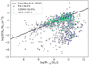 |
Fig. 1 Star formation rate vs. stellar mass integrated over each galaxy, comparing the distributions of galaxies from the CARMA and APEX subsets and the remaining CALIFA galaxies. The star formation main sequence is indicated using the Cano-Díaz et al. (2016) fit (full black line) with its confidence level (dotted black lines). The diagram is zoomed-in to emphasise the CARMA and APEX coverage. The extended CALIFA sample has SFR = 10−6.2−103.3 M⊙ yr−1 and M* = 105.7−1013.7 M⊙, however only a few objects have star formation rates and stellar mass outside the range shown in the figure. |
2.1 CALIFA data
The optical integral field spectroscopy (IFS) survey CALIFA imaged more than 1000 galaxies (667 included in the data release 3, and 416 in the extended sample) using the PMAS/PPak integral field unit instrument mounted on the 3.5 m telescope of the Calar Alto Observatory (Sánchez et al. 2012, 2016a; Lacerda et al. 2020). The CALIFA sample is drawn from the Sloan Digital Sky Survey (SDSS, York et al. 2000) to reflect the present-day galaxy population (0.005 < z < 0.03) in a statistically meaningful manner (log(M*∕[M⊙]) = 9.4–11.4; E to Sd morphologies, including irregulars, interacting, and mergers; Walcher et al. 2014; Barrera-Ballesteros et al. 2015). Here we consider the galaxies observed with the low-resolution (V500) setup, which covers between 3745 and 7500 Å with a spectral resolution FWHM = 6 Å. CALIFA data cubes possess a spatial resolution of FWHM ~ 2.5 arcsec (García-Benito et al. 2015). Given the limits on the redshift, CALIFA allows the study of galaxies on kpc scales. Additionally, the maps extend beyond 2.5 Reff, covering most of the optical discs. Ionised gas and stellar continuum map properties have been obtained through the PIPE3D pipeline (Sánchez et al. 2016b,c). PIPE3D analyses the stellar population applying the GSD156 simple stellar populations (SSP) library (Cid Fernandes et al. 2013). A stellar population fit is performed to the spatially rebinned V -band data cubes in order to estimate a spaxel-wise stellar population model. This model is used to calculate the stellar mass density value withineach spaxel. The ionised-gas data cube is then generated by subtracting the stellar population model from the original cube. Each of the 52 sets of emission line maps is performed, calculating flux intensity, centroid velocity, velocity dispersion, and equivalent width for every single spectrum.
2.2 APEX observations and survey goal
We observed the 12CO(2–1) emission (rest frequency,  = 230.538 GHz) from 296 galaxy centres and 39 off-centre positions. In this paper, we present only the centre observations. The project was carried out with the APEX 12 m sub-millimetre telescope (Güsten et al. 2006) in ON-OFF mode using the wobbler (which ensures stable baselines), and the PI230 receiver, which operates in the 1.3 mm atmospheric window. Galaxies have been observed across two projects: M9518A_130 and M9504A_104 (PI: D. Colombo), which allocated 180 and 205 h in the summer and winter semesters of 2019, respectively, for a total of approximately 385 h including calibrations, additional overheads, and further test observations. All galaxies were drawn from the CALIFA extended sample, with the only requirement to be accessible by APEX, i.e. all galaxies in the sample have declination ≤ 30°.
The APEX resolution at 230 GHz is 26.3 arcsec. The median ratio of the beam radius to the effective radius of the full sample of galaxies is 1.12, with an inter-quartile range of 0.60. These do not change much if we consider only the face-on targets (with an inclination under 65°). This means that, on average, the APEX beam covers roughly half of the radial extent of the CALIFA maps (see Sect. 2.1 and Fig. 2).
The survey is designed to reach a uniform rms of 2 mK (70 mJy) per δv = 30 km s−1 wide channels. For several targets for which we have detections but low S/N (<3), we integrate longer to achieve an rms of 1 mK. These requirements allowed us to attain pointed observations 10× more sensitive than CARMA (in terms of achievable minimum molecular gas mass surface density; see also Sect. 2.3) and thereby detect the CO line in even the most gas-poor galaxies, which constituted the main goal of our APEX observations. In particular, we obtain 207 CO detections (S∕N ≥ 3) for a detection rate of 70%, with 50% of the observed galaxies detected at 5σRMS.
Data calibration and reduction of the APEX data were performed using the Grenoble Image and Line Data Analysis Software (GILDAS1) and Continuum and Line Analysis Single-dish Software (CLASS) with which we fitted and removed a linear baseline to each spectrum outside a window of 600 km s−1 centred on the galaxy VLSR. Afterwards, we smoothed the data to a common spectral resolution, δv = 23 km s−1. The final median rms from the full sample at 23 km s−1 is 2.2 mK, which corresponds to a median, 3σRMS, Mmol = 2.8 × 10⁸ M⊙ (Σmol ~ 2.8 M⊙ pc−2) at the median distance of the sample of ~67 Mpc and using a constant αCO(2−1) = 6.23 M⊙ (K km s−1 pc2)−1. Full details about survey specifics and data reduction will be presented in an upcoming survey paper.
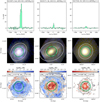 |
Fig. 2 APEX 12CO(2–1) spectra of three observed galaxies in different quenching phases. Top row panels: spectra for each galaxy in green, where the dotted line represents the observation σRMS. Top row panel: titles, the name of the galaxy (as in the CALIFA database) and its morphology, CO signal-to-noise ratio (S/N), and the logarithmic ratio of the galaxy global SFR to the global star formation main sequence (ΔSFMSg). Middle row panels: continuum RGB images extracted from the CALIFA data cubes using u- (blue), g- (green) and r- (red) bands. Bottom row: WHα maps are displayed in diverging red colours where WHα < 6 Å, while the diverging blue ones illustrate the part of the map where WHα > 6 Å. The colour maps are centred at WHα = 6 Å in logarithmic units, and this value is indicated as a black vertical line in the colour bars. Black contours mark the 25, 50, and 75 percentiles of the log(FHα) distribution,previously masked at 3σRMS. The WH α map is also masked below 3σRMS of the Hα flux map. In panel legends, the median Hα equivalent width across the whole map (⟨WHα,g⟩) and within the beam aperture (⟨WHα,b⟩) are presented. In the panels of the two bottom rows, the green circle shows the APEX beam (FWHM = 26.2 arcsec at 230 GHz), while white ellipsoids indicate 1 and 2 Reff. |
2.3 CARMA data
In addition to the APEX data, in this paper, we also make use of the CARMA database, which constitutes the first 12CO(1–0) (and 13CO(1–0)) follow-up of CALIFA galaxies undertaken by the EDGE collaboration. A full description of the CARMA CO data is given in Bolatto et al. (2017); here, we provide a brief summary. The EDGE-CALIFA collaboration originally mapped 177 infrared-bright CALIFA galaxies with CARMA E-configuration. A sub-sample of 126 higher signal-to-noise galaxies were also observed in D-configuration; subsequently, for these galaxies, D+E combined cubes were produced. In this paper, we use the 12CO(1–0) data of the 126 D+E galaxies and the remaining 51 E-configuration galaxies that were not followed up with theD-array of CARMA. The data cubes were smoothed to a spectral resolution of 20 km s−1. The final D+E galaxies have 4.5 arcsec resolution, while the E-configuration-only galaxies show a 9 arcsec resolution. The average rms noise in the D+E galaxies is 38 mK per 20 km s−1 channel width. This dataset was extensively exploited in Utomo et al. (2017), Colombo et al. (2018), Levy et al. (2018, 2019), Leung et al. (2018), Chown et al. (2019), Dey et al. (2019), and Barrera-Ballesteros et al. (2020), and recently reviewed in Sánchez (2020), exploring different aspects of the interconnection between the ionised and cold molecular gas phases in galaxies.
3 Derived quantities
In this paper, we use spatially unresolved (i.e. single-beam) data from APEX as well as resolved data from CARMA and CALIFA. In order to make these data comparable and simulate the effect the APEX beam would have on CARMA and CALIFA maps, we introduced a “tapering” function, WT, that is, a bi-dimensional Gaussian, centred on the centre of the galaxy, with unitary amplitude and FWHM θ = 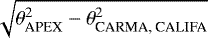 , where the APEX beam FWHM θAPEX = 26.3 arcsec, while the CARMA beam FWHM θCARMA = 4.5 arcsec or θCARMA = 9 arcsec, for the D+E or E-only configuration, respectively; and θCALIFA = 2.5 arcsec. Integrated quantities within the APEX beam aperture are indicated with the subscript, “b”, and are calculated by co-adding the pixels within the CARMA or CALIFA maps, previously multiplied by the Gaussian filter, WT. Average quantities within the APEX beam aperture are obtained using the weighted median of pixels values in the resolved maps where the weights for each pixel are given by the tapering function, WT. This operation is equivalent to the convolution of the CALIFA property maps to the APEX beam size and sampling the result at the pointing centre of the APEX beam. Globally integrated quantities, denoted with the subscript, “g”, are measured by summing up all the pixels in a given map, without applying the Gaussian taper. Where no subscript is indicated, the quantity is computed spaxel- or pixel-wise for CALIFA and CARMA maps, respectively.
3.1 CO luminosity from ON-OFF APEX observations
We derived the 12CO(2–1) flux within a spectral window of 400 km s−1 centred on the systemic velocity of the galaxy, which is derived from the stellar redshift. The CO line velocity-integrated flux is expressed by the following equation:
![Mathematical equation: \begin{equation*}S_{\textrm{CO, b}}\,\mathrm{[K\,km\,s^{-1}]}\,{=}\,\sum_i T_{\textrm{mb},i}\delta v ,\end{equation*}](/articles/aa/full_html/2020/12/aa39005-20/aa39005-20-eq3.png) (1)
(1)
where δv = 23 km s−1 is the data’s final channel width, using Tmb =  , with ηmb = 0.78 for the APEX beam efficiency at 230 GHz. SCO, b is converted to Jy km s−1 through a conversion factor between Kelvin and Jansky2 of Jy/K = 37.
The statistical error for the flux is given by
![Mathematical equation: \begin{equation*}\epsilon_{\textrm{CO, b}}\,\mathrm{[Jy\,km\,s^{-1}]}\,{=}\,\sigma_{\textrm{RMS}}\sqrt{W_{50} \delta v}. \end{equation*}](/articles/aa/full_html/2020/12/aa39005-20/aa39005-20-eq5.png) (2)
(2)
where σRMS is the standard deviation of the flux variations measured in the first and last 20 line-free channels of each spectrum: that is, measured in two spectral windows of 20 channels before and after the velocity range used to measured emission line intensities. Finally, W50 is the full width at half maximum derived as 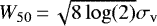 , where σv is the second moment calculated in the spectral window selected to measure the emission line (i.e. the 400 km s−1 range centred on the systemic velocity of a galaxy). The values of W50 obtained in this way coincide well with the ones derived using the “two-slopes method” presented by Springob et al. (2005) and used elsewhere (Saintonge et al. 2011, 2017; Cicone et al. 2017). For non-detected galaxies, or galaxies showing S∕N < 3, we made use of ɛCO, b to provide an upper limit for flux given by 3ɛCO, b, where we assume a constant W50 = 200 km s−1. This value was derived using the procedure described before for W50 resulting from stacking the central APEX spectra of all the APEX galaxies. This CO flux upper limit serves as a basis for calculating all other CO properties of non-detected galaxies presented here.
From the CO flux, we derived the 12CO(2–1) luminosity using Eq. (3) of Solomon et al. (1997):
![Mathematical equation: \begin{equation*}L_{\textrm{CO, b}}\,\mathrm{[K\,km\,s^{-1}\,pc^2]}\,{=}\,3.25\,{\times}\,10^7\frac{D_{\textrm{L}}^2}{\nu_{\textrm{obs}}^2 (1+z)^3}S_{\textrm{CO, b}} ,\end{equation*}](/articles/aa/full_html/2020/12/aa39005-20/aa39005-20-eq7.png) (3)
(3)
where DL is the luminosity distance in Mpc (derived from the stellar redshift, z), νobs is the observed frequency of the emission line in the rest frame in GHz, and SCO, b is the CO velocity-integrated flux derived using Eq. (1) (but in Jy km s−1).
3.2 CO luminosity from CARMA data cubes
The 12CO(1–0) CARMA observations in the original EDGE database comes as position-position-velocity data cubes. Therefore, we used the tapering function, WT, here. For the CARMA data, the CO velocity-integrated intensity within the APEX beam aperture is given by:
![Mathematical equation: \begin{equation*}I_{\textrm{CO, b}}\,\mathrm{[K\,km\,s^{-1}]}\,{=}\,\sum_i I_{\textrm{CO},i}\,{\times}\,W_{\textrm{T}}(x_i, y_i), \end{equation*}](/articles/aa/full_html/2020/12/aa39005-20/aa39005-20-eq8.png) (4)
(4)
where the summation runs on the bi-dimensional pixels of the integrated intensity map ICO of the whole galaxy. After this, the CO luminosity within the APEX beam aperture is calculated by
![Mathematical equation: \begin{equation*}L_{\textrm{CO, b}}\,\mathrm{[K\,km\,s^{-1}\,pc^2]}\,{=}\,I_{\textrm{CO, b}}\,\delta x\, \delta y\, (1+z)^{-1}, \end{equation*}](/articles/aa/full_html/2020/12/aa39005-20/aa39005-20-eq9.png) (5)
(5)
where δx, δy are the pixel sizes in pc, and z is the galaxy redshift.
As in Sect. 3.1, we provide an upper limit for the CO flux-related quantities of the non-detected galaxies (S∕N < 3) as 3ɛCO given by Eq. (2), where we assume a constant W50 = 200 km s−1. For detected targets, the full width at half maximum, W50, of the line that enters in the calculation of the flux statistical error, ɛCO, is obtained forthe CARMA galaxies from the CO spectrum built using the integrated flux in each channel map.
3.3 Molecular gas mass and αCO
The molecular gas mass follows from the CO luminosity by assuming a CO-to-H2 conversion factor, αCO, b:
 (6)
(6)
For the CARMA CO(1−0) data, we used αCO, b ≡ αCO(1-0), b (Bolatto et al. 2017). However, for the APEX observations, an additional correction factor is required, with αCO, b = αCO(1-0), b∕R21, where R21 is the CO(2–1)/CO(1–0) ratio. This value is determined to be ~0.7 in nearby galaxies (Leroy et al. 2013; Saintonge et al. 2017).
Given that our sample consists of a variety of galaxies often quite far from the star formation main sequence, here we assume a variable αCO(1-0) based on Bolatto et al. (2013), Eq. (31):
![Mathematical equation: \begin{equation*}\alpha_{\textrm{CO(1{-}0)}}\,[M_{\odot}\,(\textrm{K\,km\,s}^{-1}\,\textrm{pc}^{2})^{-1}]\,{=}\,2.9\exp\left(\frac{0.4}{Z'}\right) \left(\!\frac{\Sigma_{\textrm{*}}}{100\,{M_{\odot}\,\textrm{pc}^{-2}}}\!\right)^{-\gamma} \!,\end{equation*}](/articles/aa/full_html/2020/12/aa39005-20/aa39005-20-eq11.png) (7)
(7)
where Z′ is the gas-phase metallicity relative to solar metallicity, Σ* is the stellar mass surface density measured at each pixel in the CALIFA data, and γ = 0.5 where Σ* > 100 M⊙ pc−2 (or γ = 0 otherwise). Unlike Bolatto et al. (2013), to avoid iterative solving here we simply assumed that Σtotal ≡ Σ*, since for our sample galaxies the gas mass surface density is generally one order of magnitude lower than the stellar mass surface density. Also,  , the giant molecular cloud’s (GMC) molecular gas mass surface density in units of 100 M⊙ pc−2, does not appear in Eq. (7), as we assume
  here, considering that the GMC molecular gas mass surface density in the inner regions of nearby galaxies and the Milky Way is largely consistent with 100 M⊙ pc−2 (see Sun et al. 2018; Colombo et al. 2019). For galaxies where optical emission lines remain undetected, we assume Z′ = 1. Details on the Z′ and Σ* calculation are given in Sect. 3.4. In Eq. (7), αCO is calculated across the whole CALIFA map; within the APEX beam aperture, we used the weighted median from the CO-to-H2 conversion factor map, αCO, b, where the weights for each pixel are given by the tapering function, WT.
Using this method, we derived a median  3.93 M⊙ (K km s−1 pc2)−1 with an inter-quartile range
  2.04 M⊙ (K km s−1 pc2)−1 for the new dataset observed with APEX. In contrast, for the CARMA dataset we obtain
  (K km s−1 pc2)−1 and
  1.23M⊙ (K km s−1 pc2)−1. Those values are a few times lower than the canonical αCO(1-0) = 4.35 M⊙ (K km s−1 pc2)−1 and αCO(2-1) = 6.21M⊙ (K km s−1 pc2)−1 of the Milky Way, possibly due to the fact that the stellar mass surface density in the centre of our sample galaxies (which extend to massive red sequence galaxies) is typically higher than in the Milky Way and generally in star-forming galaxies, while the gas-phase metallicity of most of our galaxies is close to solar.
3.4 IFS-derived parameters
For the purpose of this work, we made use of both nebular lines and stellar-continuum-derived maps provided by CALIFA data. In particular, we used Hα, Hβ, [OIII] λ5007, and [NII] λ6583 flux maps (defined as FHα, FH β, F[OIII], and F[NII], respectively); the Hα equivalent width (WHα) maps; and the stellar mass surfacedensity (Σ*) maps.
We calculated the extinction-corrected SFR spaxel-by-spaxel using the nebular extinction based on the Balmer decrement:
![Mathematical equation: \begin{equation*}A_{\textrm{H}\alpha}\,\mathrm{[Mag]}\,{=}\,\frac{K_{\textrm{H}\alpha}}{0.4(K_{\textrm{H}\beta} - K_{\textrm{H}\alpha})}\,{\times}\, \log\left(\frac{F_{\textrm{H}\alpha}}{2.86 F_{\textrm{H}\beta}}\right), \end{equation*}](/articles/aa/full_html/2020/12/aa39005-20/aa39005-20-eq18.png) (8)
(8)
where the coefficients KHα = 2.53 and KHβ = 3.61 follow the Cardelli et al. (1989) extinction curve (see also Catalán-Torrecilla et al. 2015).
The SFR is then computed as:
![Mathematical equation: \begin{equation*}\mathrm{SFR}\,{[M_{\odot}\,\textrm{yr}^{-1}]}\,{=}\,8\,{\times}\, 10^{-42} F_{\textrm{H}\alpha}\,{\times}\, 10^{A_{\textrm{H}\alpha}/2.5}, \end{equation*}](/articles/aa/full_html/2020/12/aa39005-20/aa39005-20-eq19.png) (9)
(9)
as indicated by Kennicutt (1998), which assumes the Salpeter initial mass function (Salpeter 1955). To obtain the integrated SFR within the APEX beam aperture, we coadded all spaxels where WH α > 6 Å. In regions where WH α < 6 Å, the Hα flux is not due to recent star formation but is dominated by the old stellar population or other effects (Sánchez et al. 2013; Espinosa-Ponce et al. 2020). Additionally, we removed all spaxels from the summation where the ionisation is due to AGN (i.e. all the spaxels that fall above the BPT diagram, Baldwin et al. 1981, demarcation line given by Kewley et al. 2001 in their Eq. (5)). We distinguish between the beam SFR, SFRb = ∑i SFRi × WT,i, as the integrated SFR within the APEX beam aperture, and the global SFR, SFRg = ∑iSFRi, as the co-addition of pixels over the whole map.
The beam stellar mass, M*,b = ∑i M*,i × WT,i, is obtained in the same way by the summation of the stellar masses from the spaxels within the APEX beam aperture, while the global stellar mass, M*,glob = ∑i M*,i, is given by the summation over the whole map. In these formulae, the index i runs over the spaxels of the entire maps, and the quantities without subscripts indicate the respective CALIFA data-derived maps.
To calculate αCO within the APEX beam aperture, we measured the gas-phase metallicity over the CALIFA maps using the O3N2 method (Marino et al. 2013):
![Mathematical equation: \begin{equation*}12 + \log\left(\frac{\textrm{O}}\textrm{H}\right)\,{=}\,8.533 - 0.214\,{\times}\, \log\left(\frac{F_{\textrm{[OIII]}}}{F_{\textrm{H}\beta}} \frac{F_{\textrm{H}\alpha}}{F_{\textrm{[NII]}}}\right). \end{equation*}](/articles/aa/full_html/2020/12/aa39005-20/aa39005-20-eq20.png) (10)
(10)
As before, the median gas-phase metallicity within the APEX beam aperture is calculated assuming the weights given by the Gaussian filter, WT. Using this method, we obtain a median of 8.43 dex from the full galaxy sample, with an inter-quartile range of 0.07 dex. The median metallicity with respect to the Solar metallicity (8.69; Allende Prieto et al. 2001) is  .
.
Lastly, we calculated the SFE and the molecular gas mass fraction (with respect to the stellar mass) within the APEX beam aperture, respectively, using:
![Mathematical equation: \begin{equation*}\mathrm{SFE_b}\,[\textrm{yr}^{-1}]\,{=}\,\mathrm{SFR_b}/M_{\textrm{mol,b}}, \end{equation*}](/articles/aa/full_html/2020/12/aa39005-20/aa39005-20-eq22.png) (11)
(11)
 (12)
(12)
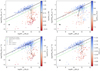 |
Fig. 3 SFR-M* diagrams integrated over CALIFA FoV, colour-coded by the median of the following quantities calculated in the APEX beam as described in the text: (a) median Hα equivalent width (⟨WHα,b⟩); (b) molecular gas mass (Mmol, b); (c) star formation efficiency (SFEb); and (d) fraction of molecular gas with respect to the stellar mass (fmol, b). The solid black line indicates the SFMS fit by Cano-Díaz et al. (2016) with its confidence level (dotted lines). The green dashed line is 3σ (0.6 dex) below the SFMS fit, which we assume indicates the start of the “green valley”. In each panel, circles indicate CO detections (S∕N ≥ 3), and triangles non-detections (S∕N < 3). Panel c: unfilled symbols show data with SFE~0 (i.e. SFR~0) within the APEX beam aperture (see text for further details). The squares illustrate the position of the average M* and SFR at four different percentile ranges of the colouring parameter (<25%, 25–50%, 50–75% and >75%), with their colours indicating the average value at each percentile range. The error bar in the bottom right of each panel shows the average errors of the reported parameters. The black horizontal line in the colour bar of panel a indicates the demarcation ⟨WH α,b⟩ = 6 Å value in logarithmic units. |
4 Results
4.1 The SFR–M* diagram
Figure 3 displays the distribution of galaxies across the SFR-M* diagram using SFR and M* measurements integrated over the entire CALIFA field of view (FoV), SFRg, and M*, g, respectively.Each panel illustrates a different quantity calculated over the APEX beam aperture. Quantities shown include: (a) equivalent width of Hα (⟨WHα,b⟩), (b) molecular gas mass (Mmol, b), (c) SFEb, and (d) theratio of molecular gas mass to stellar mass (molecular gas mass fraction fmol, b), respectively. On average, the CALIFA maps extend to approximately 2 Reff, while the APEX beam covers the inner 1 Reff of the galaxies (see Fig. 2). The measurements within the APEX beam aperture can be considered, therefore, as inner galaxy measurements. In addition, we include the SFMS fit derived by Cano-Díaz et al. (2016) (log (SFR) = (0.81 ± 0.02)log(M*) − (8.34 ± 0.19)) to illustrate the location of the star-forming galaxies across this diagram. In the following, we provide the Pearson and Spearman correlation coefficients r as rp and rs, respectively. For all correlation discussed in the paragraphs we obtain an extremely low p-value ≪ 10−16.
Global star-forming galaxies can be largely separated from galaxies on the way to quenching using a threshold given by ⟨WHα,b⟩ = 6 Å, that is, by considering the quenching stage of their centres. Panel a of Fig. 3, where the data points are colour-coded by ⟨WHα,b⟩, shows that most galaxies where this value is above 6 Å are tightly distributed along the SFMS locus defined by the Cano-Díaz et al. (2016) fit. We consider the lower boundary of the SFMS to be 3σ (~ 0.6 dex) below the fit, which encompasses ~99% of the galaxies dominated by star formation in their centres (which show similar medians ⟨WHα,b⟩ and ⟨WHα,g⟩ around 13 Å). However, we still observe ~ 25% of the centrally retired galaxy sub-sample (with ⟨WHα,b⟩ < 6 Å) above this line. Those galaxies have median ⟨WHα,b⟩~ 4.3 Å and median ⟨WHα,g⟩~ 5.3 Å, which is quite close to our threshold of 6 Å, and they are mostly star forming in their outskirts but not in their centres.
It is interesting to note that quenched objects still possess a significant amount of molecular gas in their centres (Fig. 3b). In particular, we see objects with high or average values of this quantity well within the green valley and the red sequence; for example, 22 galaxies with Mmol,b values above the 75th percentile of its distribution are below 3σ from the SFMS fit. At the opposite extreme, 46 objects with Mmol,b values belowthe 25th percentile of the Mmol,b distribution are above the dashed green line defining galaxies within 3σ of the SFMS fit. Figure 3b shows that Mmol,b is directly related to the globalSFR and M*, but correlates more tightly with the SFRg (given rp = 0.65 and rs = 0.73) than with M*, g (rp = 0.46 and rs = 0.33).
The SFE in the centre of the galaxies varies widely across the SFR–M* diagram. However, it appears roughly constant along the SFMS, but it drops sharply right below it (panel c). Quantitatively,  yr−1 and
  yr−1 above the green valley boundary, while below it,
  yr−1 and
  yr−1. In other words, galaxies below the main sequence show, on average, depletion times a factor of five longer than galaxies across the SFMS in their central regions. Additionally, we have a few galaxies that do not appear to form stars in their centres (R < Reff), resulting in SFE~0 in the aperture defined by the APEX beam. Those are galaxies with Hα flux below the detection limit, or their Hα map spaxels are masked since WH α < 6 Å. Nevertheless, most of these galaxies do have a few star-forming regions in the outskirts, typically outside the circle defined by their Reff (such as NGC 0171 in Fig. 2). Some of these galaxies are non-detected in CO (nine targets): therefore, the absence of recent star formation could be directly attributed to the absence of molecular gas (in the matched aperture). However, some of the SFE~0 galaxies are detected in CO (five targets), meaning that the star formation quenching at the centre is due to causes other than a simple shortage of raw fuel. As for Mmol,b, we also observe a few galaxies with SFEb much lower than the sample average very close to the main sequence (five targets with SFEb below the 25th percentile of the SFE distribution are above the 3σ line). SFEb decreases with stellar mass (as also observed in Colombo et al. 2018 with a limited sample of EDGE galaxies; see their Fig. 3, panel d). The SFEs in the galaxy centres appear quite strongly correlated with SFRg (given rp = 0.73 and rs = 0.46), but only moderately with M*, g (rp = −0.38 and rs = −0.53). The SFEb reaches very low values; however, those values are generally SFEb lower limits that are mostly driven by CO non-detected galaxies, for which we use an Mmol, b upper limit to calculate SFEb.
The molecular-gas-mass-to-stellar-mass ratio, fmol,b, shows a general behaviour across the SFR-M* diagram that is quite similar to SFEb (panel d). As for SFEb, fmol,b is largely constant along the SFMS and sharply decreases below the SFMS. Quantitatively,  and
and  above the green valley boundary, and
  and
and  below it. We observe galaxies along and below the main sequence with fmol,b values much lower and much higher than the sample average. In particular, we have 14 targets with fmol,b below the 25th percentile of the distribution above the 3σ line (dashed green line) from the SFMS fit, while five objects with fmol,b values above the 75th are located below this line. Nevertheless, the molecular-gas-mass-to-stellar-mass ratio appears only moderately correlated with SFRg (rp = 0.50 and rs = 0.50) and M*, g (rp = −0.44 and rs = −0.50).
4.2 What quenches galaxies: variable SFE or a shortage of molecular gas?
Star formation quenching can be parameterised using the logarithmic difference between the observed SFR and the SFR expected from the best fit to the SFMS, ΔSFMS (e.g. Genzel et al. 2015; Tacconi et al. 2018; Ellison et al. 2018; Thorp et al. 2019). In panels a and b of Fig. 4, we plot Δ SFMSg with respect to SFEb and fmol,b, respectively,in order to understand whether the star formation quenching is more tightly connected to variations in SFE or to the absence of molecular gas in galaxy centres. This is basically a reorganisation of the star formation mass diagram presented in Fig. 3, removing the dependence of SFR on M* (i.e. the SFMS trend). As before, SFEb and fmol,b are measured within the APEX beam aperture, while Δ SFMSg uses the SFR and M* measured over the entire CALIFA map. Following the arguments discussed for Fig. 3 (panel a), we divided the sample into two sub-samples based on the average WH α within the APEX beam aperture (⟨WHα,b⟩): galaxies largely quenched in the centre (⟨WHα,b⟩ < 6 Å) and galaxies dominated by star formation in their centres (⟨WHα,b⟩ > 6 Å). The two sub-samples are well balanced in terms of target size. There are 256 centrally star-forming galaxies (i.e. ~ 54% of the full sample), while the centrally retired galaxies constitute ~46% of the sample (i.e. 216 objects).
The behaviour of Δ SFMSg versus SFEb is somehow similar for the two sub-samples. The Δ SFMSg–SFEb relationship measured using the principal component analysis (PCA; see Colombo et al. 2018) shows that the slope from the confidence ellipsoids between the two sub-samples is on the same order of ~ 0.3 for centrally star-forming galaxies and ~0.6 for centrally quenched galaxies (see Table 1, where the Spearman correlation coefficients rs are reported for the two sub-samples).
Nevertheless, data points for star-forming galaxies are tightly concentrated close to the SFMS and have SFEb values from 10−10−10−8 yr−1 (i.e. τdep = 0.1−10 Gyr). By contrast, quenched galaxies cover a much larger parameter space in both Δ SFMSg and SFEb, in particular, they span six orders of magnitudes in SFE. Additionally, Δ SFMSg and SFEb appear strongly correlated, showing a Pearson rp = 0.9. However, this tight correlation is mostly driven by the centrally quenched galaxies, for which rp = 0.8, while for the star-forming targets rp = 0.2, which indicates that Δ SFMSg and SFEb are basically uncorrelated for this kind of object, and the calculated slope of the relationship is meaningless. The SFE in our centrally star-forming galaxies is quite constant, in line with results from several other resolved and unresolved studies of nearby, star-forminggalaxies. We also note that the values of the correlation coefficients do not change significantly for the Δ SFMSg -SFEb and Δ SFMSg -fmol,b relationships if only the detected targets are considered (Table 1).
On the other hand, the slopes of relationship between Δ SFMSg and fmol,b are starkly different if we consider the star-forming and quenched targets separately. Galaxies largely quenched in the centre span a few orders of magnitude in Δ SFMSg as well as in fmol,b. Indeed, the PCA shows that in quenched galaxies there is a steep relationship between Δ SFMSg and fmol,b (with a slope of ~3.15). However, this correlation is shallower for galaxies with central star formation activity (slope ~ 0.64). They have fmol,b approximately one order of magnitude larger than for centrally quenched galaxies (⟨log(fmol,b)⟩ = −1.77 for centrally star-formingand ⟨log(fmol,b)⟩ = −2.51 for centrallyretired objects; see Table 1).
Nevertheless, the Pearson correlation coefficients are lower with respect to the SFE case: for the full sample, we observe rp = 0.7, while for the two sub-samples separately we observe a similar rp ~ 0.5. This indicates that, in contrast to the SFE case, for both centrally star-forming and quenched targets Δ SFMSg and fmol,b are moderately correlated. Those conclusions do not change significantly if only the CO-detected galaxies are considered (see Fig. 4 and Table 1).
It is worth noting that the SFEb exhibits a bimodal distribution similar to the one found for Δ SFMSg (i.e. values of SFEb below 10−10 yr−1 are almost exclusively associated with quenched targets). By contrast, a bimodal distribution is not evident for fmol,b, for which the difference in fmol,b between centrally star-forming and retired objects is not as sharp. Additionally, the bimodality in SFEb and Δ SFMSg is driven by the same group of galaxies. In other words, centrally star-forming and retired galaxy sub-groups are equally well separated in Δ SFMSg and in SFEb. Thus, SFE in the galaxy centres (in particular retired centres) is a better predictor of the separation between the two groups than the respective fmol,b.
The histograms of Δ SFMSg, SFEb, and fmol,b colour-coded by ⟨WHα,b⟩ in a given bin, are shown in panels c–e. Generally, the median of global Δ SFMSg (− 0.3) and beam SFEb (~ 4.4 × 10⁻⁹ yr) are close to the values of these parameters that separate star-forming and quenched galaxies (i.e. ΔSFMS(WHα = 6 Å) and SFE(WHα = 6 Å)). In particular, the median SFE corresponds to a τdep = 2.3 Gyr, which is equivalent to the value measured from kpc-resolved EDGE objects (see Utomo et al. 2017; Colombo et al. 2018)and other nearby spiral galaxies (Leroy et al. 2013). However, the median of the beam fmol,b (~ 10−2) distribution is shifted towards the retired sub-sample as this value is slightly below the demarcation, fmol,b, which separates centrally star-forming and quiescent galaxies (fmol,b(WHα = 6 Å) = 10−1.95).
Summary of the PCA fit of the ΔSFMSg- log(SFEb) and ΔSFMSg- log(fmol,b) relationships for centrally star-forming (⟨WHα,b⟩ > 6 Å) and centrally retired galaxies (⟨WHα,b⟩ < 6 Å) (or globally star-forming, ⟨WHα,g⟩ > 6 Å, and globally retired galaxies, ⟨WHα,g⟩ < 6 Å) for different galaxy sub-samples or quantity calculations.
5 Discussion and conclusions
In this paper, we used 472 galaxies to test whether the star formation quenching of CALIFA galaxies is mostly due to changes in the SFE or to the absence of molecular gas (as described by the ratio between the molecular and stellar gas masses, fmol) in their centres.
We observe that for galaxies dominated by star formation activity in their centres, distance from the main sequence correlates better with the molecular-to-stellar-mass ratio. For centrally quiescent galaxies, instead, distance from the main sequence correlates better with SFE. This suggests a scenario where the progressive loss of the cold gas reservoir is what causes galaxies to move out of the main sequence. Once this happens, the star formation efficiency in the remaining cold gas reser voir is what modulates their retirement, with lower efficiencies corresponding to more quiescent galaxies. In this scenario, both amount to (molecular) gas and SFE matter, but they have different roles. In particular, the stabilisation of the molecular gas reservoir plays a role once the galaxy enters the green valley, but it is less important than the size of the reservoir in moving the galaxy out of the main sequence. Furthermore, this quenching happens from the inside out, with centrally quenched galaxies leading the path towards totally quenched ones. Those results do not change significantly if we consider a constant αCO instead of our preferred αCO from Eq. (7) to convert CO luminosity to molecular gas mass, or if we divide the full sample using the value of the Hα equivalent width obtained over the entire maps, or if only the APEX sub-sample of galaxies is used (see Table 1).
The importance of the absence of molecular gas for understanding why some galaxies are located far from the SFMS has been acknowledged in the past from other (integrated, but aperture-limited) studies that used a direct molecular gas tracer as CO, in both the local and higher redshift Universe. At z ~ 0, a series of papers using the COLDGASS3 and xCOLDGASS4 samples (Saintonge et al. 2012, 2016, 2017) have shown that variations of the specific star formation rate (sSFR = SFR/M*) can be almost fully described by variations in gas fractions (especially molecular gas fraction), but the relation between fmol and sSFR is not linear, meaning that variations in star formation efficiency (which appears almost constant with the stellar mass, cf. Saintonge et al. 2016) also play a role. Similar results are obtained by extending the sample to higher redshift (up to z ~ 4 Genzel et al. 2015).
A relatively inexpensive way to explore the distribution of molecular gas in galaxies is to use indirect proxies. In particular, the dust-to-gas relation can be applied to estimate both the integrated Mmol and its distribution across galaxies. A recent calibrator proposed by Barrera-Ballesteros et al. (2020) was used in Sánchez et al. (2018) and Lacerda et al. (2020) to explore the radial distribution of the molecular gas and its integrated molecular gas mass for different galaxy morphologies. They confirm the results by Colombo et al. (2018) in terms of the variation of the SFE across galaxy types and stellar masses, despite the limitations of the adopted estimators. Furthermore, Sánchez et al. (2018) used two large samples of IFS spatially resolved observations comprising 2700 galaxies from the MaNGA5 (Bundy et al. 2015) IFS survey (and 8000 galaxies from a large IFS compilation) to confirm that the SFE decreases as galaxies move from the MS to the retired galaxy regime, going through the green valley (see their Figs. 8 and 11), as recently reviewed by Sánchez (2020, their Fig. 18). Like in the case of the (x)COLDGASS results, they attribute this to the lack of gas and not the low SFE, which is the primary cause of the cessation of star formation.
Similarly, Piotrowska et al. (2020), using a dust-to-gas calibrator method to analyse ~ 62 000 SDSS DR7 local galaxies, found that (independently from the stellar mass) both decreasing gas supply and decreasing efficiency are important to define the distance from the star formation main sequence, in line with the previously discussed integrated study results. Tacconi et al. (2018) used both CO and dust-extrapolated molecular gas masses in the redshift range z = 0−4, and they also confirmed the primary dependency of sSFR to fmol with a weaker contribution from SFE changes (see also Scoville et al. 2016).
The same question was recently addressed using spatially resolved measurements. Ellison et al. (2020) used 34 galaxies from the ALMaQUEST6 sample that images MaNGA targets in 12CO(1–0) with the Atacama Large Millimeter/submillimeter Array (ALMA). This sample also includes green valley targets. They find that on kpc-scales, variations in SFE (measured as ΣSFR∕Σmol), rather than resolved fmol changes (calculated from Σmol∕Σ*), drive the SFR surface density of galaxies away from the “resolved” star formation main sequence (Lin et al. 2019). By analysing seven green valley galaxies, Brownson et al. (2020) found that SFE and fmol appear equally important to explain quenching in the outer regions of galaxies. However, they were unable to establish which is the dominant mechanism in the galaxy centres, which appear strongly quenched in their sample. They indicated that, while low fmol values seem to drive the quenching in the inner regions, reduced SFE could also play a role. Through a smaller sample of nearby galaxies, but observed at a higher resolution, Morselli et al. (2020) noticed that changes in the total gas fraction (calculated including the contribution of the atomic gas) are more significant than the total SFE in explaining distance from the resolved SFMS for star-forming galaxies, as we observe here using integrated measurements.
Integrated CO surveys cannot reach the level of detail regarding the molecular gas organisation achieved by kpc-resolved studies. But they do provide the ability to obtain samples that are several times larger, as well as the possibility to detect galaxies with much less molecular gas over a shorter observing time. In this paper, we give the first presentation of a new integrated CO survey using APEX that follows up CALIFA targets. Once completed, this survey will give 12 CO(2–1) (and possibly also 13CO(2–1) and C18O(2–1) for the brightest targets) observations of 450 CALIFA galaxy centres and a few off-centre detections. Thus, the size of this survey is similar to that of the most recent explorations at redshift ~ 0, like xCOLDGASS (532 galaxies), but with aperture-matched optical spectroscopic data (not restricted to the central 3″, which could cause several issues in the classification of the ionisation stages, Sánchez 2020), and for a much narrower range of cosmological distances (i.e. with less bias introduced by possible cosmological evolution). The survey is unbiased by construction, with its only requirement being that the targets are observable by APEX (δ < 30°). Together with CARMA data, we will collect CO data for ~630 galaxies fully covered by high-resolution IFS information, providing the largest CO database of any major IFS survey to date.
Nonetheless, to fully exploit the IFS information and take the next step in understanding the mechanisms that drive these galaxy changes requires high-resolution interferometric gas imaging of the sample, something that needs to be strongly supported by proper time allocation.
Indeed, ALMA would be particularly appropriate for this scope. Within our centrally quenched sample, we measure a median molecular gas mass upper limit Mmol ~ 108 M⊙, within a 26.3 arcsec APEX beam. A short (~20 min) integration on CO(2–1) emission over the full disc of a CALIFA galaxy with ALMA 12 m array would provide a 1σ sensitivity of ~ 8.7 mJy in 1 km s−1 channel. This is equivalent to Σmol ~ 2 M⊙ pc−2 for 30 km s−1-wide lines, which would correspond to a Mmol ≃ 106.2 M⊙ for the median distance to CALIFA galaxies, in a beam that matches the CALIFA resolution (~ 3 arcsec). Therefore, a short integration with ALMA has a 5σ limit of Mmol ~ 107 M⊙ (depending on the precise distance and line width of the target), and would be able to significantly improve our limits and potentially resolve the faint CO emission of a quenched galaxy. At these integration times, large surveys are possible, so about 300 CALIFA targets could be done in approximately 100 h. This would provide a representative and invaluable high-resolution sample of galaxies to study the star formation quenching process in the local Universe.
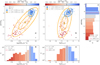 |
Fig. 4 Offset from main sequence for a galaxy (ΔSFMSg) versus star formation efficiency (SFEb, panel a) and versus the molecular gas fraction inside the APEX beam (fmol, b, panel b) colour-coded by the median Hα equivalent width (⟨WHα,b⟩) within the APEX beam aperture. In the two panels, circles represent CO detections (S∕N ≥ 3), while triangles indicate CO upper limits (S∕N < 3). Error bars at the bottom right of each figure represent the typical uncertainties of the represented parameters. The two sub-samples include galaxies largely retired in the centre (⟨WH α,b⟩ < 6Å), or dominated by star formation (⟨WHα,b⟩ > 6Å), following the results of Fig. 3. The squares represent the median values of the represented parameters for the two sub-samples, while the ellipses correspond to the shape of the distribution derived using the PCA analysis described in the text, and contain approximately 1 and 2σ of the data within the two sub-samples. Dotted-line ellipses are obtained including only CO detections, while solid-line ellipses correspond to the full sample (which also includes CO upper limits). Due to the different dynamical range of the x- and y-axes, some ellipses could be distorted, therefore the dashed coloured lines clarify the principalcomponent direction for the full sub-samples. In the legend, the formulae indicate the linear fits derived from the two sub-samples using the PCA analysis and rp, the respective Pearson correlation coefficients. Panels c–e: histogram distributions of ΔSFMSg, SFEb, and fmol,b, respectively colour-encoded by the average ⟨WHα,b⟩ in each bin. The dashed line indicates the median of the distribution (μ), while the dotted lines the interquartile range (σ). The red line indicates the value of the quantity at the demarcation value given by ⟨WH α,b⟩ = 6 Å (i.e. the separation between centrally star-forming and retired galaxies). The black vertical line in the colour bars of panels a and b indicates the demarcation ⟨WH α,b⟩ = 6 Å value in logarithmic units. |
Acknowledgements
The authors thank the anonymous referee for the constructive report. D.C. and A.W. acknowledges support by the Deutsche Forschungsgemeinschaft, DFG project number SFB956A. S.F.S. thanks the support of Coancyt grants FC2016-01-1916 and CB-285080, and UNAM-DGAPA-PAPIIT IA100519. E.R. acknowledges the support of the Natural Sciences and Engineering Research Council of Canada (NSERC), funding reference number RGPIN-2017-03987. A.D.B., T.W., L.B., S.V., and R.C.L. acknowledge support from the National Science Foundation (NSF) through collaborative research award AST-1615960. T.W. and Y.C. acknowledge support from the NSF through grant AST-1616199. J.B.B. acknowledges support from the grant IA-100420 (PAPIIT-DGAPA, UNAM). This research made use of Astropy (http://www.astropy.org) a community-developed core Python package for Astronomy (Astropy Collaboration 2013, 2018); matplotlib (Hunter 2007); numpy and scipy (Virtanen et al. 2020). Support for CARMA construction was derived from the Gordon and Betty Moore Foundation, the Eileen and Kenneth Norris Foundation, the Caltech Associates, the states of California, Illinois, and Maryland, and the NSF. Funding for CARMA development and operations were supported by NSF and the CARMA partner universities.
References
- Abadi, M. G., Moore, B., & Bower, R. G. 1999, MNRAS, 308, 947 [NASA ADS] [CrossRef] [Google Scholar]
- Alatalo, K., Davis, T. A., Bureau, M., et al. 2013, MNRAS, 432, 1796 [NASA ADS] [CrossRef] [Google Scholar]
- Allende Prieto, C., Lambert, D. L., & Asplund, M. 2001, ApJ, 556, L63 [Google Scholar]
- Astropy Collaboration (Robitaille, T. P., et al.) 2013, A&A, 558, A33 [NASA ADS] [CrossRef] [EDP Sciences] [Google Scholar]
- Astropy Collaboration (Price-Whelan, et al.) 2018, AJ, 156, 123 [Google Scholar]
- Baldwin, J. A., Phillips, M. M., & Terlevich, R. 1981, PASP, 93, 5 [NASA ADS] [CrossRef] [EDP Sciences] [Google Scholar]
- Barrera-Ballesteros, J. K., García-Lorenzo, B., Falcón-Barroso, J., et al. 2015, A&A, 582, A21 [NASA ADS] [CrossRef] [EDP Sciences] [Google Scholar]
- Barrera-Ballesteros, J. K., Utomo, D., Bolatto, A. D., et al. 2020, MNRAS, 492, 2651 [CrossRef] [Google Scholar]
- Bigiel, F., Leroy, A., Walter, F., et al. 2008, AJ, 136, 2846 [NASA ADS] [CrossRef] [Google Scholar]
- Bigiel, F., Leroy, A. K., Walter, F., et al. 2011, ApJ, 730, L13 [NASA ADS] [CrossRef] [Google Scholar]
- Bolatto, A. D., Wolfire, M., & Leroy, A. K. 2013, ARA&A, 51, 207 [Google Scholar]
- Bolatto, A. D., Wong, T., Utomo, D., et al. 2017, ApJ, 846, 159 [NASA ADS] [CrossRef] [Google Scholar]
- Brinchmann, J., Charlot, S., White, S. D. M., et al. 2004, MNRAS, 351, 1151 [NASA ADS] [CrossRef] [Google Scholar]
- Brownson, S., Belfiore, F., Maiolino, R., Lin, L., & Carniani, S. 2020, MNRAS, 498, L66 [CrossRef] [Google Scholar]
- Bundy, K., Bershady, M. A., Law, D. R., et al. 2015, ApJ, 798, 7 [NASA ADS] [CrossRef] [Google Scholar]
- Cano-Díaz, M., Sánchez, S. F., Zibetti, S., et al. 2016, ApJ, 821, L26 [NASA ADS] [CrossRef] [Google Scholar]
- Cardelli, J. A., Clayton, G. C., & Mathis, J. S. 1989, ApJ, 345, 245 [NASA ADS] [CrossRef] [Google Scholar]
- Catalán-Torrecilla, C., Gil de Paz, A., Castillo-Morales, A., et al. 2015, A&A, 584, A87 [NASA ADS] [CrossRef] [EDP Sciences] [Google Scholar]
- Chown, R., Li, C., Athanassoula, E., et al. 2019, MNRAS, 484, 5192 [CrossRef] [Google Scholar]
- Cicone, C., Maiolino, R., Sturm, E., et al. 2014, A&A, 562, A21 [NASA ADS] [CrossRef] [EDP Sciences] [Google Scholar]
- Cicone, C., Bothwell, M., Wagg, J., et al. 2017, A&A, 604, A53 [Google Scholar]
- Cid Fernandes, R., Pérez, E., García Benito, R., et al. 2013, A&A, 557, A86 [NASA ADS] [CrossRef] [EDP Sciences] [Google Scholar]
- Colombo, D., Kalinova, V., Utomo, D., et al. 2018, MNRAS, 475, 1791 [NASA ADS] [CrossRef] [Google Scholar]
- Colombo, D., Rosolowsky, E., Duarte-Cabral, A., et al. 2019, MNRAS, 483, 4291 [NASA ADS] [CrossRef] [Google Scholar]
- Davis, T. A., Young, L. M., Crocker, A. F., et al. 2014, MNRAS, 444, 3427 [NASA ADS] [CrossRef] [Google Scholar]
- Dekel, A., & Birnboim, Y. 2006, MNRAS, 368, 2 [NASA ADS] [CrossRef] [Google Scholar]
- Dekel, A., & Silk, J. 1986, ApJ, 303, 39 [NASA ADS] [CrossRef] [Google Scholar]
- Dey, B., Rosolowsky, E., Cao, Y., et al. 2019, MNRAS, 488, 1926 [CrossRef] [Google Scholar]
- Donovan Meyer, J., Koda, J., Momose, R., et al. 2013, ApJ, 772, 107 [NASA ADS] [CrossRef] [Google Scholar]
- Ellison, S. L., Sánchez, S. F., Ibarra-Medel, H., et al. 2018, MNRAS, 474, 2039 [NASA ADS] [CrossRef] [Google Scholar]
- Ellison, S. L., Thorp, M. D., Lin, L., et al. 2020, MNRAS, 493, L39 [CrossRef] [Google Scholar]
- Espinosa-Ponce, C., Sánchez, S. F., Morisset, C., et al. 2020, MNRAS, 494, 1622 [CrossRef] [Google Scholar]
- Faber, S. M., Willmer, C. N. A., Wolf, C., et al. 2007, ApJ, 665, 265 [NASA ADS] [CrossRef] [Google Scholar]
- García-Benito, R., Zibetti, S., Sánchez, S. F., et al. 2015, A&A, 576, A135 [NASA ADS] [CrossRef] [EDP Sciences] [Google Scholar]
- Genzel, R., Tacconi, L. J., Lutz, D., et al. 2015, ApJ, 800, 20 [Google Scholar]
- González Delgado, R. M., Cid Fernandes, R., Pérez, E., et al. 2016, A&A, 590, A44 [NASA ADS] [CrossRef] [EDP Sciences] [Google Scholar]
- Güsten, R., Nyman, L. Å., Schilke, P., et al. 2006, A&A, 454, L13 [NASA ADS] [CrossRef] [EDP Sciences] [Google Scholar]
- Hunter, J. D. 2007, Comput. Sci. Eng., 9, 90 [NASA ADS] [CrossRef] [Google Scholar]
- Kennicutt, Jr., R. C. 1998, ApJ, 498, 541 [NASA ADS] [CrossRef] [Google Scholar]
- Kewley, L. J., Dopita, M. A., Sutherland, R. S., Heisler, C. A., & Trevena, J. 2001, ApJ, 556, 121 [Google Scholar]
- Kirkpatrick, A., Pope, A., Aretxaga, I., et al. 2014, ApJ, 796, 135 [CrossRef] [Google Scholar]
- Koyama, S., Koyama, Y., Yamashita, T., et al. 2019, ApJ, 874, 142 [CrossRef] [Google Scholar]
- Lacerda, E. A. D., Sánchez, S. F., Cid Fernandes, R., et al. 2020, MNRAS, 492, 3073 [Google Scholar]
- Leroy, A. K., Walter, F., Brinks, E., et al. 2008, AJ, 136, 2782 [Google Scholar]
- Leroy, A. K., Bolatto, A., Bot, C., et al. 2009, ApJ, 702, 352 [Google Scholar]
- Leroy, A. K., Walter, F., Sandstrom, K., et al. 2013, AJ, 146, 19 [Google Scholar]
- Leroy, A. K., Bolatto, A. D., Ostriker, E. C., et al. 2015, ApJ, 801, 25 [NASA ADS] [CrossRef] [Google Scholar]
- Leung, G. Y. C., Leaman, R., van de Ven, G., et al. 2018, MNRAS, 477, 254 [NASA ADS] [CrossRef] [Google Scholar]
- Levy, R. C., Bolatto, A. D., Teuben, P., et al. 2018, ApJ, 860, 92 [NASA ADS] [CrossRef] [Google Scholar]
- Levy, R. C., Bolatto, A. D., Sánchez, S. F., et al. 2019, ApJ, 882, 84 [CrossRef] [Google Scholar]
- Lin, L., Belfiore, F., Pan, H.-A., et al. 2017, ApJ, 851, 18 [NASA ADS] [CrossRef] [Google Scholar]
- Lin, L., Pan, H.-A., Ellison, S. L., et al. 2019, ApJ, 884, L33 [NASA ADS] [CrossRef] [Google Scholar]
- Marino, R. A., Rosales-Ortega, F. F., Sánchez, S. F., et al. 2013, A&A, 559, A114 [NASA ADS] [CrossRef] [EDP Sciences] [Google Scholar]
- Martig, M., Bournaud, F., Teyssier, R., & Dekel, A. 2009, ApJ, 707, 250 [NASA ADS] [CrossRef] [Google Scholar]
- Meidt, S. E., Schinnerer, E., García-Burillo, S., et al. 2013, ApJ, 779, 45 [NASA ADS] [CrossRef] [Google Scholar]
- Mok, A., Wilson, C. D., Golding, J., et al. 2016, MNRAS, 456, 4384 [NASA ADS] [CrossRef] [Google Scholar]
- Moore, B., Katz, N., Lake, G., Dressler, A., & Oemler, A. 1996, Nature, 379, 613 [NASA ADS] [CrossRef] [Google Scholar]
- Morselli, L., Rodighiero, G., Enia, A., et al. 2020, MNRAS, 496, 4606 [CrossRef] [Google Scholar]
- Muraoka, K., Sorai, K., Miyamoto, Y., et al. 2019, PASJ, 71, S15 [CrossRef] [Google Scholar]
- Piotrowska, J. M., Bluck, A. F. L., Maiolino, R., Concas, A., & Peng, Y. 2020, MNRAS, 492, L6 [Google Scholar]
- Rahman, N., Bolatto, A. D., Wong, T., et al. 2011, ApJ, 730, 72 [NASA ADS] [CrossRef] [Google Scholar]
- Rahman, N., Bolatto, A. D., Xue, R., et al. 2012, ApJ, 745, 183 [NASA ADS] [CrossRef] [Google Scholar]
- Regan, M. W., Thornley, M. D., Helfer, T. T., et al. 2001, ApJ, 561, 218 [NASA ADS] [CrossRef] [Google Scholar]
- Renzini, A., & Peng, Y.-j. 2015, ApJ, 801, L29 [NASA ADS] [CrossRef] [Google Scholar]
- Rosario, D. J., Burtscher, L., Davies, R. I., et al. 2018, MNRAS, 473, 5658 [NASA ADS] [CrossRef] [Google Scholar]
- Saintonge, A., Kauffmann, G., Wang, J., et al. 2011, MNRAS, 415, 61 [NASA ADS] [CrossRef] [Google Scholar]
- Saintonge, A., Tacconi, L. J., Fabello, S., et al. 2012, ApJ, 758, 73 [Google Scholar]
- Saintonge, A., Catinella, B., Cortese, L., et al. 2016, MNRAS, 462, 1749 [Google Scholar]
- Saintonge, A., Catinella, B., Tacconi, L. J., et al. 2017, ApJS, 233, 22 [Google Scholar]
- Salim, S., Rich, R. M., Charlot, S., et al. 2007, ApJS, 173, 267 [NASA ADS] [CrossRef] [Google Scholar]
- Salpeter, E. E. 1955, ApJ, 121, 161 [Google Scholar]
- Sánchez, S. F. 2020, ARA&A, 58, 99 [CrossRef] [Google Scholar]
- Sánchez, S. F., Kennicutt, R. C., Gil de Paz, A., et al. 2012, A&A, 538, A8 [NASA ADS] [CrossRef] [EDP Sciences] [Google Scholar]
- Sánchez, S. F., Rosales-Ortega, F. F., Jungwiert, B., et al. 2013, A&A, 554, A58 [NASA ADS] [CrossRef] [EDP Sciences] [Google Scholar]
- Sánchez, S. F., García-Benito, R., Zibetti, S., et al. 2016a, A&A, 594, A36 [NASA ADS] [CrossRef] [EDP Sciences] [Google Scholar]
- Sánchez, S. F., Pérez, E., Sánchez-Blázquez, P., et al. 2016b, Rev. Mex. Astron. Astrofis., 52, 21 [NASA ADS] [Google Scholar]
- Sánchez, S. F., Pérez, E., Sánchez-Blázquez, P., et al. 2016c, Rev. Mex. Astron. Astrofis., 52, 171 [Google Scholar]
- Sánchez, S. F., Avila-Reese, V., Hernandez-Toledo, H., et al. 2018, Rev. Mex. Astron. Astrofis., 54, 217 [Google Scholar]
- Scoville, N., Sheth, K., Aussel, H., et al. 2016, ApJ, 820, 83 [NASA ADS] [CrossRef] [Google Scholar]
- Solomon, P. M., Downes, D., Radford, S. J. E., & Barrett, J. W. 1997, ApJ, 478, 144 [NASA ADS] [CrossRef] [Google Scholar]
- Sorai, K., Kuno, N., Muraoka, K., et al. 2019, PASJ, 71, S14 [Google Scholar]
- Springob, C. M., Haynes, M. P., Giovanelli, R., & Kent, B. R. 2005, ApJS, 160, 149 [Google Scholar]
- Sun, J., Leroy, A. K., Schruba, A., et al. 2018, ApJ, 860, 172 [NASA ADS] [CrossRef] [Google Scholar]
- Tacconi, L. J., Genzel, R., Saintonge, A., et al. 2018, ApJ, 853, 179 [NASA ADS] [CrossRef] [Google Scholar]
- Thorp, M. D., Ellison, S. L., Simard, L., Sánchez, S. F., & Antonio, B. 2019, MNRAS, 482, L55 [CrossRef] [Google Scholar]
- Utomo, D., Bolatto, A. D., Wong, T., et al. 2017, ApJ, 849, 26 [CrossRef] [Google Scholar]
- Virtanen, P., Gommers, R., Oliphant, T. E., et al. 2020, Nat. Methods, 17, 261 [Google Scholar]
- Walcher, C. J., Wisotzki, L., Bekeraité, S., et al. 2014, A&A, 569, A1 [NASA ADS] [CrossRef] [EDP Sciences] [Google Scholar]
- Whitaker, K. E., van Dokkum, P. G., Brammer, G., & Franx, M. 2012, ApJ, 754, L29 [NASA ADS] [CrossRef] [Google Scholar]
- Wilson, C. D., Warren, B. E., Israel, F. P., et al. 2009, ApJ, 693, 1736 [NASA ADS] [CrossRef] [Google Scholar]
- York, D. G., Adelman, J., Anderson, Jr., J. E., et al. 2000, AJ, 120, 1579 [CrossRef] [Google Scholar]
CO legacy database for the GASS survey.
Extended CO legacy database for the GASS survey.
Mapping nearby galaxies at Apache Point Observatory.
ALMA-MaNGA QUEnching and STar formation.
All Tables
Summary of the PCA fit of the ΔSFMSg- log(SFEb) and ΔSFMSg- log(fmol,b) relationships for centrally star-forming (⟨WHα,b⟩ > 6 Å) and centrally retired galaxies (⟨WHα,b⟩ < 6 Å) (or globally star-forming, ⟨WHα,g⟩ > 6 Å, and globally retired galaxies, ⟨WHα,g⟩ < 6 Å) for different galaxy sub-samples or quantity calculations.
All Figures
|
Fig. 1 Star formation rate vs. stellar mass integrated over each galaxy, comparing the distributions of galaxies from the CARMA and APEX subsets and the remaining CALIFA galaxies. The star formation main sequence is indicated using the Cano-Díaz et al. (2016) fit (full black line) with its confidence level (dotted black lines). The diagram is zoomed-in to emphasise the CARMA and APEX coverage. The extended CALIFA sample has SFR = 10−6.2−103.3 M⊙ yr−1 and M* = 105.7−1013.7 M⊙, however only a few objects have star formation rates and stellar mass outside the range shown in the figure. |
| In the text | |
|
Fig. 2 APEX 12CO(2–1) spectra of three observed galaxies in different quenching phases. Top row panels: spectra for each galaxy in green, where the dotted line represents the observation σRMS. Top row panel: titles, the name of the galaxy (as in the CALIFA database) and its morphology, CO signal-to-noise ratio (S/N), and the logarithmic ratio of the galaxy global SFR to the global star formation main sequence (ΔSFMSg). Middle row panels: continuum RGB images extracted from the CALIFA data cubes using u- (blue), g- (green) and r- (red) bands. Bottom row: WHα maps are displayed in diverging red colours where WHα < 6 Å, while the diverging blue ones illustrate the part of the map where WHα > 6 Å. The colour maps are centred at WHα = 6 Å in logarithmic units, and this value is indicated as a black vertical line in the colour bars. Black contours mark the 25, 50, and 75 percentiles of the log(FHα) distribution,previously masked at 3σRMS. The WH α map is also masked below 3σRMS of the Hα flux map. In panel legends, the median Hα equivalent width across the whole map (⟨WHα,g⟩) and within the beam aperture (⟨WHα,b⟩) are presented. In the panels of the two bottom rows, the green circle shows the APEX beam (FWHM = 26.2 arcsec at 230 GHz), while white ellipsoids indicate 1 and 2 Reff. |
| In the text | |
|
Fig. 3 SFR-M* diagrams integrated over CALIFA FoV, colour-coded by the median of the following quantities calculated in the APEX beam as described in the text: (a) median Hα equivalent width (⟨WHα,b⟩); (b) molecular gas mass (Mmol, b); (c) star formation efficiency (SFEb); and (d) fraction of molecular gas with respect to the stellar mass (fmol, b). The solid black line indicates the SFMS fit by Cano-Díaz et al. (2016) with its confidence level (dotted lines). The green dashed line is 3σ (0.6 dex) below the SFMS fit, which we assume indicates the start of the “green valley”. In each panel, circles indicate CO detections (S∕N ≥ 3), and triangles non-detections (S∕N < 3). Panel c: unfilled symbols show data with SFE~0 (i.e. SFR~0) within the APEX beam aperture (see text for further details). The squares illustrate the position of the average M* and SFR at four different percentile ranges of the colouring parameter (<25%, 25–50%, 50–75% and >75%), with their colours indicating the average value at each percentile range. The error bar in the bottom right of each panel shows the average errors of the reported parameters. The black horizontal line in the colour bar of panel a indicates the demarcation ⟨WH α,b⟩ = 6 Å value in logarithmic units. |
| In the text | |
|
Fig. 4 Offset from main sequence for a galaxy (ΔSFMSg) versus star formation efficiency (SFEb, panel a) and versus the molecular gas fraction inside the APEX beam (fmol, b, panel b) colour-coded by the median Hα equivalent width (⟨WHα,b⟩) within the APEX beam aperture. In the two panels, circles represent CO detections (S∕N ≥ 3), while triangles indicate CO upper limits (S∕N < 3). Error bars at the bottom right of each figure represent the typical uncertainties of the represented parameters. The two sub-samples include galaxies largely retired in the centre (⟨WH α,b⟩ < 6Å), or dominated by star formation (⟨WHα,b⟩ > 6Å), following the results of Fig. 3. The squares represent the median values of the represented parameters for the two sub-samples, while the ellipses correspond to the shape of the distribution derived using the PCA analysis described in the text, and contain approximately 1 and 2σ of the data within the two sub-samples. Dotted-line ellipses are obtained including only CO detections, while solid-line ellipses correspond to the full sample (which also includes CO upper limits). Due to the different dynamical range of the x- and y-axes, some ellipses could be distorted, therefore the dashed coloured lines clarify the principalcomponent direction for the full sub-samples. In the legend, the formulae indicate the linear fits derived from the two sub-samples using the PCA analysis and rp, the respective Pearson correlation coefficients. Panels c–e: histogram distributions of ΔSFMSg, SFEb, and fmol,b, respectively colour-encoded by the average ⟨WHα,b⟩ in each bin. The dashed line indicates the median of the distribution (μ), while the dotted lines the interquartile range (σ). The red line indicates the value of the quantity at the demarcation value given by ⟨WH α,b⟩ = 6 Å (i.e. the separation between centrally star-forming and retired galaxies). The black vertical line in the colour bars of panels a and b indicates the demarcation ⟨WH α,b⟩ = 6 Å value in logarithmic units. |
| In the text | |
Current usage metrics show cumulative count of Article Views (full-text article views including HTML views, PDF and ePub downloads, according to the available data) and Abstracts Views on Vision4Press platform.
Data correspond to usage on the plateform after 2015. The current usage metrics is available 48-96 hours after online publication and is updated daily on week days.
Initial download of the metrics may take a while.