| Issue |
A&A
Volume 699, July 2025
|
|
|---|---|---|
| Article Number | A195 | |
| Number of page(s) | 10 | |
| Section | The Sun and the Heliosphere | |
| DOI | https://doi.org/10.1051/0004-6361/202453071 | |
| Published online | 07 July 2025 | |
Untwisting motion and bidirectional outflows of a filament
1
School of Space Science and Technology, and Institute of Space Sciences, Shandong University, Weihai 264209, China
2
School of Astronomy and Space Science and Key Laboratory of Modern Astronomy and Astrophysics, Nanjing University, Nanjing 210023, PR China
3
Observatoire de Paris, LIRA, Université PSL, CNRS, Sorbonne Université, Université de Paris, 5 place Jules Janssen, F-92190 Meudon, France
4
University of Glasgow, School of Physics and Astronomy, Glasgow, G128QQ Scotland, UK
5
Centre for mathematical Plasma Astrophysics, Dep. of Mathematics, KU Leuven, 3001 Leuven, Belgium
6
Key Laboratory of Solar Activity, National Astronomical Observatories, Chinese Academy of Sciences, Beijing 100012, PR China
⋆ Corresponding author: This email address is being protected from spambots. You need JavaScript enabled to view it.
Received:
19
November
2024
Accepted:
6
May
2025
Abstract
Context. Filament consists of cold and dense plasma that is suspended in the corona. Observations with a high spatial resolution indicate that its fine structure is highly dynamic during its evolution and eruption.
Aims. We wish to understand the mechanism that produces twisting motions and bidirectional outflows in filaments by combining observation and simulation.
Methods. The filament evolution was observed in multiple wavelengths by the New Vacuum Solar Telescope (NVST), the Solar Upper Transition Region Imager (SUTRI), the Chinese Hα Solar Explorer (CHASE), the Atmospheric Imaging Assembly (AIA), and the Helioseismic and Magnetic Imager (HMI) on board the Solar Dynamic Observatory (SDO). A data-constrained magnetohydrodynamic (MHD) 3D simulation was performed to explain the physical phenomena behind the observations.
Results. We report untwisting motions in a filament and its bidirectional outflows before and after a B8.4 X-ray flare. Before the flare, magnetic reconnection between threads occurred in the middle part of the filament, which resulted in the rise and oscillations of the filament. Brightenings in AIA 304 Å and AIA 171 Å in the interaction region were registered. After about 40 minutes, the right branch of the filament showed untwisting motions and bidirectional outflows in Hα as measured by time-distance diagrams and Dopplergrams of NVST. the MHD simulations showed that during the rising phase of the right branch of the flux rope (FR), magnetic reconnection of the sheared arcades below the flux rope occured that increased the FR twist. Magnetic reconnection induced bidirectional outflows and increased the plasma density in the FR by levitation.
Conclusions. The 3D data-based MHD simulations confirmed that the bidirectional outflows observed in the NVST Hα filament were caused by magnetic reconnection. During the reconnection, plasma is injected, which leads to the dense observed filament with a high opacity in CHASE observations.
Key words: Sun: activity / Sun: filaments / prominences / Sun: magnetic fields
© The Authors 2025
 Open Access article, published by EDP Sciences, under the terms of the Creative Commons Attribution License (https://creativecommons.org/licenses/by/4.0), which permits unrestricted use, distribution, and reproduction in any medium, provided the original work is properly cited.
This article is published in open access under the Subscribe to Open model. This email address is being protected from spambots. You need JavaScript enabled to view it. to support open access publication.
1. Introduction
Prominences are cold (104° K) and dense plasma (1010 cm−3) that is suspended in the hot corona (106° K) with a density of (108 cm−3). Prominences projected onto the solar surface that are observed in the Hα line appear as black filaments because their radiation is weaker than the background (Martin 1998; Ruan et al. 2018, 2019a; Chen et al. 2020). In addition to the Hα spectral lines, which are commonly used for observing filaments, the filaments can also be observed in some chromospheric spectral lines such as Ca II and Mg II and in some extreme-ultraviolet (EUV) wavelengths and radio wavelengths (Schmieder et al. 2003, 2004a, 2014). The filaments lie above the polarity-inversion lines that separate the positive and negative polarities (PILs; Babcock & Babcock 1955; Martin 1998). Filaments consist of a spine, which is the main core of the filament, and of lateral barbs, which appear as footpoints or anchorage of the filament in the low atmosphere. Many different classifications have been proposed based on the shape, movement characteristics, and location of the filaments. The most common classifications are active region filaments, quiescent filaments, and intermediate filaments, according to their location. Eruptive filaments are often thought to be the bright cores of typical coronal mass ejections (CMEs) (Schmieder 2006).
The magnetic configuration of filaments in the corona plays a crucial role in the understanding of the formation, evolution, and eruption of filaments. Based on theories and numerical simulations, two classical models of filament magnetic structure have been proposed: the Kippenhahn-Schlüter model (Kippenhahn & Schlüter 1957) and the Kuperus-Raadu model (Kuperus & Raadu 1974). However, in an actual observation, the filaments are complex and variable, and on this basis, the sheared arcade model (DeVore & Antiochos 2000; Aulanier & Schmieder 2002; Welsch et al. 2005) and the flux rope model (Amari et al. 2000; Aulanier et al. 2010; Guo et al. 2010; Cheng et al. 2014) were proposed. In the magnetic structure of a filament, flux rope, or arcade, the cool material is located in the dips of shallow twisted or sheared magnetic field lines (Aulanier & Demoulin 1998; Aulanier et al. 1998). The Lorentz force (upward magnetic tension) is balanced by the gravity of the plasma of which the filament consists. With the improving resolution of solar telescopes, a deeper understanding of the dynamic filament evolution was possible. The high-resolution observations revealed that the plasma flows dynamically along the filament threads. A counterstream moves in opposite directions in the adjacent filament threads. This was first observed by Zirker et al. (1998) using high-resolution Hα images from Big Bear Solar Observatory (BBSO; Goode & Cao 2012). The authors found that the plasma flows were in the opposite direction in the Hα blue- and red-wing observations and were present in the spine and the barbs. The velocity of these counterstreams was 5–20 km/s. Lin et al. (2008) found a velocity of the counterstream as high as 25 km/s in active regions. Moreover, Alexander et al. (2013) detected that the velocity of the counterstream of 193 Å in the active region was 70–80 km/s, which is higher than in Hα observations. Diercke et al. (2018) observed counterstreams in 171 Å, 193 Å, 304 Å, and 211 Å by using a contrast-enhancement technique, so that these flows could be detected and quantifıed with local correlation tracking (LCT; November & Simon 1988). One of the explanations for the cause of the counterstream is the longitudinal oscillation of the filament (Lin et al. 2005; Xia et al. 2011). Another possible explanation is that the heating of the chromosphere at the two footpoints of the filament threads is asymmetric, which causes the counterstream. If the heating of the chromosphere is random, then the counterstream occurs in the overall filament thread observation (Chen et al. 2014).
Yokoyama & Shibata (1996) pointed out that the two-sided-loop jet takes places between the emerging flux and the coronal magnetic field with a characteristic of a pair of horizontal jets. Ruan et al. (2019b) found the signal of bidirectional reconnection outflows by using data from spectra observed with the Interface Region Imaging Spectrograph (IRIS; De Pontieu et al. 2014). Bidirectional outflows are evidence of magnetic reconnection (Savage et al. 2010; Su et al. 2013; Zhu et al. 2016).
Filaments sometimes exist in a very specific form called double-decker filaments. These may consist of two branches that are distributed at different heights, but they are all along the same PIL (Liu et al. 2012). When the filaments are disturbed, they become unstable and may erupt, and they may be accompanied by other solar activities such as flares (Wang et al. 2005, 2006; Ruan et al. 2015; Song et al. 2018; Yan et al. 2018, 2022; Kumar et al. 2024; Liu et al. 2024a), CMEs (Ruan et al. 2014; Feng et al. 2015; Chen et al. 2016; Liu et al. 2024b; Song et al. 2024; Zhang et al. 2015; Hou et al. 2024), EUV waves (Zheng et al. 2022; Dai et al. 2023), jets (Sterling et al. 2015; Ruan et al. 2019b; Yang et al. 2024), and radio bursts (Zhang et al. 2022; Liu et al. 2024b). When the filaments erupt but the material cannot escape into the interplanetary space, they are called failed eruptions (Ji et al. 2003). Filaments may undergo magnetic reconnection during their evolution (Schmieder et al. 2004b, 2006; Zhou et al. 2017). Filaments sometimes move in an interesting way during their evolution. They rotate (Su et al. 2014; Zhou et al. 2019; Guo et al. 2023, 2024a), twist or untwist (Schmieder et al. 1985; Li & Zhang 2013; Wang et al. 2015; Xue et al. 2016; Xu et al. 2020), merge (Schmieder et al. 2004b; Su et al. 2007; Li et al. 2023) and writhe (Liu et al. 2008; Xu et al. 2020).
The triggering mechanisms of filament eruptions have been discussed for a long time, and they are now generally divided into ideal magnetohydrodynamic instabilities (Bi et al. 2015; Mei et al. 2018) and magnetic reconnection (Chen & Shibata 2000; Schmieder & Aulanier 2012; Shen et al. 2012; Chen et al. 2014; Schmieder et al. 2016; Zheng et al. 2017; Hou et al. 2019; Ruan et al. 2019b; Yan et al. 2020; Li et al. 2022b; Sun et al. 2023; Xue et al. 2023; Hou et al. 2023; Liu et al. 2024b). Usually, one of the triggering mechanisms plays a role in the filament eruption, and sometimes, both are involved (Song et al. 2015).
We present two bidirectional outflows of a right-branch filament accompanied by a B-class flare. The evolution of the filament was observed by the New Vacuum Solar Telescope (NVST; Liu et al. 2014), the Solar Upper Transition Region Imager (SUTRI; Bai et al. 2023), the Chinese Hα Solar Explorer (CHASE; Li et al. 2022a), and the Solar Dynamics Observatory (SDO; Pesnell et al. 2012). We describe this in Sections 2 and 3. In Section 5, we perform an MHD simulation to reproduce the evolution of the filament after the merging of two segments, which explains the observed outflows. The aim of the paper is to understand the origin of the bidirectional outflows in the filament and the untwisted motion prior the eruption by using data-based MHD simulations.
2. Observation
The NVST is a 1 m vacuum solar telescope and is located in the Fuxian Solar Observatory of the Yunnan Observatories, Chinese Academy of Sciences (CAS). The NVST Hα data used here were obtained at the line center (6562.8 Å) and in the line wings (6562.8 ± 0.8 Å) with a spatial resolution of 0.″165 pixel−1 and a temporal resolution of 78 s from 06:16:25 UT to 08:52:39 UT. The Dopplergrams were constructed based on the above Hα data by using the following equation (Langangen et al. 2008):
 (1)
(1)
where B and R represent the blue-wing (Hα −0.8 Å) and the red-wing (Hα +0.8 Å) data. It is important to note that the Dopplergrams only represent the Doppler shift signal and not the exact Doppler velocity. The positive (negative) Doppler index D corresponds to the Doppler redshift (blueshift).
SUTRI provides solar disk images on board the first spacecraft of the Space Advanced Technology demonstration satellite series (SATech-01), Chinese Academy of Sciences (CAS). The images we used were taken from the solar atmosphere at a temperature of 0.5 MK using the Ne VII 46.5 nm line from 07:01:41 UT to 07:55:41 UT. The SUTRI data have a cadence of 30 s and a spatial resolution of 1.″23 per pixel.
CHASE is the first solar space mission of the China National Space Administration (CNSA). The Hα Imaging Spectrograph (HIS) is the scientific payload of the CHASE satellite. It consists of two observational modes: a raster-scanning mode, and a continuum-imaging mode. The data we used are the full-disk spectral images provided by the former from 08:18:14 UT to 08:44:16 UT. The Hα data (6559.7–6565.9 Å) and Fe I data (6567.8–6570.6 Å) have a spatial resolution of 1.″04 per pixel and a temporal resolution of 1 min. The spectral resolution of the binning-mode data is 0.048 Å pixel−1.
The Atmospheric Imaging Assembly (AIA; Lemen et al. 2012) and the Helioseimic and Magnetic Imager (HMI; Schou et al. 2012) on board the SDO provide the EUV coronal images and photospheric line-of-sight magnetograms during the evolution of the filament. The AIA EUV passbands of 304 Å, 171 Å, 193 Å, 211 Å, 335 Å, 131 Å, and 94 Å have a pixel resolution of 0.″6 and a temporal resolution of 12 s. HMI data has a pixel size of 0.″5 and a cadence of 45 s. We coaligned the data from different instruments according to the cross-correlation technique by capturing common features of sunspots and filaments in each frame.
3. Results
We report that the right branch of a filament showed bidirectional outflows during the filament evolution twice. This event occurred on 2 November 2022 for the target of active region NOAA 13135, while at the same time, a B8.4 X-class flare was observed in this region. During this time, some very bright flare loops were visible in 131 Åand 94 Å of the AIA, but were not visible in the lower-temperature spectral lines. The evolution of the filament was analyzed in detail using simultaneous observations from SDO, SUTRI, NVST, and CHASE.
The filament was located in the northern hemisphere roughly in the center of the solar disk. Figure 1 shows the multiwavelength observations, where the field of view of NVST observation is shown as the dashed green box in panel e. The active region consisted of two major sunspots with negative polarity on the left and positive polarity on the right, where the filament was rooted. There are also some mixed polarities between them distributed north-south. The elongated filament was distributed over these polarities and connected the two main sunspots. The orange box R1 in the magnetogram indicates the region of the right branch of the filament we studied (as shown in Figures 3 and A.1). With the onset of the flare, flare ribbons were observed in the EUV channels and in the Hα bands. Some bright coronal loops are only visible in the images of 131 Å and 94 Å. The high-resolution observations of NVST clearly show the fine thread structure of the filament.
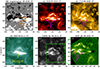 |
Fig. 1. Overview of multiwavelength observations in active region AR 13135. Panels (a)–(d) show a map of the magnetic field (HMI) and three intensity maps in 304 Å, 171 Å, and 94 Å from AIA. Panel (e) and panel (f) show Hα observations of CHASE in black and white and NVST in green, respectively. The Hα observation of NVST is the enlarged area of the dashed green box in panel (e). The orange box in the magnetogram (panel a) indicates the region of the right branch of the filament (box R1). The position of the filament is indicated by magenta arrows F in panel b and coronal loops by a yellow arrow in panel d. The associated movie is available online (aa53071-24movie.mp4). |
Before the flare, interactions of filament threads were observed by NVST and AIA. The middle part of the filament was initially stable, but after some disturbances, it rose around 07:00 UT. The magnetic flux evolution increased in positive flux from the time marked by the green arrow in Figure 5, panel d. This means that the magnetic emergence and magnetic cancellation were related to this disturbance and promoted the rising and untwisting motion of the filament. Subsequently, the light curve in R2 slightly increased (see the dashed black box R4 in panel e of Figure 5). In the Doppler velocity map sequence (doppler_fov.mp4), the filament apex exhibits blueshifted signatures around x = −160″, y = 373″, indicating a vertical velocity component in the thread dynamics. The slice S1 along the direction of the rising threads shows that the threads reached the highest point at about 07:09 UT. At the same time, there are significant brightenings at 304 Å and 171 Å in Figure 2, which coincide with the footpoints of the threads after magnetic reconnection. In addition, the merged magnetic flux rope becomes looser, and the blue and orange lines indicate visibly loose threads in Figure 2, panel d. The green contour connects the two ends of the dashed magenta and yellow lines at 07:09:29 UT. The differently colored dashed lines stand for different threads involved in the interaction. Panels a and d in Figure 2 show that the two threads originally separated and then merged after magnetic reconnection. Corresponding to the magnetogram, it is the left footpoint of the dashed magenta line connected to the right footpoint of the dashed yellow line. After the interaction between threads, the filament oscillated, as shown in Figure 2, panel f.
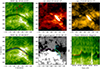 |
Fig. 2. Temporal evolution of the middle part of filament at two times (panel a at 07:01:41 UT and panel d at 07:09:26 UT): Zoom of the central NVST image in Hα of Figure 1. The NVST intensity of Hα is shown in green. In panel (d) the blue and orange lines represent the composition of the magnetic flux rope after magnetic reconnection. Panels (b) and (c) show the corresponding brightening in the AIA 304 Åand 171 Å images. Panel (e) shows the corresponding magnetogram. The dashed magenta and yellow lines represent the interacting threads at 07:01:41 UT. The green contour represents the brightening of 304 Å at 07:09:29 UT. The cyan box (R2) represents the area of the calculated magnetic flux shown in Figure 5. In panel (f) we show the time–distance diagram of the slice S1 shown in panel (a). The movement of the threads is indicated by the dashed red line. |
Figure 3 shows the process of untwisting motion of the right branch of the filament, which occurred before the B8.4 X-class flare in the region of R1 (marked by the orange box in Figure 1). At 07:41:47 UT, the threads of the filament moved in the direction opposite to the direction of the twist compared to the previous moment. This branch gradually became looser in the next few minutes, and the twisted structure graduallydisappeared. The high-resolution observations of NVST clearly show the changes in these threads. During this time, these threads continually brightened in AIA 304 Å, and the bright blobs on the threads gradually moved to the west (green arrow in Figure 3). The brightening also appeared in other EUV bands, which correspond to the radiation enhancement marked by the dashed black box R3 in Figure 5 panel c. During this time, bidirectional outflows were observed in Hα, 304 Å, and 465 Å, shown in Figure 4 along slice S2. It is hard to see direct evidence of magnetic reconnection in observations. There is much evidence that helps to prove that magnetic reconnection occurs, such as changes in the magnetic field connectivity, plasma inflow and outflow, magnetic emergence and cancellation, magnetic shear and transient brightening, as documented in observations by high-resolution instruments. In the case of two-dimensional magnetic reconnection, bidirectional outflows can be generated (Priest 2014). Around 07:40 UT, bidirectional outflows are represented by the green and red lines, which indicate magnetic reconnection. The velocity of these outflows was between 15 and 80 km/s. The Hα off-band ±0.8 Å images were used to construct the Dopplergrams. At 07:39:56 UT, threads at the position of y = 357″ ∼360″ are blueshifted in Figure 3, panel (c1), and the threads then gradually became redshifted in panel (c3), indicating that they moved in the opposite direction. This change in the direction of motion corresponded to the untwisting process and bidirectional outflows of the threads.
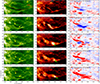 |
Fig. 3. Untwisting motion evolution of the filament, right branch, observed by the NVST in the Hα line center and by AIA in 304 Å between 07:40 UT and 07:45 UT before the flare. The yellow arrows indicate the threads that untwist and become loose. The observations of NVST are presented in panels (a1)–(a5), in 304 Å in panels (b1)–(b5), reconstructed Dopplergrams in panels (c1)–(c5) (blue and red correspond to blue- and redshift). The curved red arrow in panel (a) represents slice S2, along which the plasma flows. The green arrows in the 304 images indicate the brightening blobs that move west. |
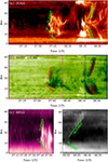 |
Fig. 4. Time–distance diagrams along the filament (S2 slice shown in Figure 3a) in AIA 304 Å, in NVST Hα, in SUTRI 465 Å, and in CHASE Hα intensity images. They show bidirectional outflows during the filament evolution. The flow velocities are overlaid on the diagrams. The dashed magenta box represents the time range of SUTRI 465 Å, and the dashed blue box shows the time range of CHASE Hα in panel (b). |
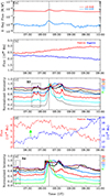 |
Fig. 5. Panel (a) shows the GOES SXR 0.5–4.0 Å and 1–8 Å flux variation and reveals the B8.4 flare. Panels (b) and (d) show the magnetic flux evolution of R1 and R2 (marked by orange and blue boxes in Figures 1 and 2), respectively. The positive (red) and negative (blue) flux are plotted. Panels (c) and (e) show light curves of the EUV channels in R1 and R2 using different colors. The vertical black line represents the peak time of the flare. The green arrow and R4 stand for the time of disturbance of the middle part of the filament. Panel (b) shares a common y-axis for the positive and negative magnetic flux. In panel (d), the values of positive and negative magnetic flux differ significantly, so that the positive values use the left y-axis and the negative values use the right y-axis. R3 covers the time of the untwisting motion of the right branch of the filament before the flare. |
During the evolution of the filament, a B8.4 X-class flare was observed with a peak time of 08:14 UT shown in Figure 5. Panel a shows the soft X-ray flux map, whose flux peak reached the B level. Panels b and d show the curves of positive and negative flux evolution in the areas of R1 and R2, respectively. For the middle part of the filament, the positive and negative fluxes have an overall decreasing trend with time in panel d. However, the positive magnetic flux has a prominent increasing change around 06:40 UT. We already discussed the effect of this change on the filament threads. For the right branch of the filament, the positive flux gradually increased, but the negative flux gradually decreased in panel b. This tendency indicates that there was a continuous magnetic emergence and magnetic cancellation, which can promote magnetic reconnection. Panels c and e show plots of the evolution of the EUV radiation intensity with time in regions R1 and R2, respectively. There is a radiative enhancement in the EUV bands during the rising and untwisting motion process of the threads in these two areas at different times.
The observation of CHASE was made after the flare. Bidirectional outflows are also visible in Hα of CHASE in the right branch of the filament. Figure 6 illustrates the dynamics and spectral properties of the right branch of the filament after the flare. Point P is on the filament spine, and the spectral profiles of it at different times are shown in panel b. During the event, the profiles show deeper line centers with time in panel b. The spectrum-time diagram of P is shown in panel c, and the result shows that the intensity here gradually decreased with time. This means that the plasma accumulated during this period. Panel e shows the spectrum of a path along the spine (see the dashed cyan lines in Figure 6, panel a) at 08:20:36 UT. A blueshift and redshift are visible at the vertical black line, which stands for the position of point P. These upward and downward outflows indicate magnetic reconnection.
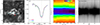 |
Fig. 6. Observation of CHASE at 08:26:33 UT. The dashed cyan line represents the path along the spine of the filament, and a red point P is on it. Spectrum profiles of point P at different times are shown in panel (b), and the black line represents the line profile of the quiet region. Panel (c) shows the spectrum-time diagram of point P. Panel (d) shows the spectrum along the path at 08:20:36 UT. The vertical black line represents the position of point P. |
4. Observational data-based MHD modeling
After the middle part of the filament reconnected, it became the whole filament (Figure 2). To investigate the physical details behind observations, we performed an MHD simulation based on observational data to model the dynamic evolution of the coronal magnetic fields. The initial magnetic fields and bottom boundary were derived or provided by observed vector magnetograms, so that they were directly comparable to observations (Guo et al. 2019, 2024a; Schmieder et al. 2024; Guo et al. 2024b). Similar to Guo et al. (2019) and Guo et al. (2021), we used a zero-β MHD model to simulate the evolution of the coronal magnetic fields, and the governing equations were
 (2)
(2)
 (3)
(3)
 (4)
(4)
where ρ denotes the density, v the velocity, and B the magnetic fields. The initial magnetic fields were provided by nonlinear force-free-field (NLFFF) modeling, and the initial density including a chromosphere and corona is consistent with Guo et al. (2019). Regarding the bottom boundary in ghost cells, the magnetic fields were constrained by the vector magnetograms, the density was fixed at the initial value, and the velocity of the cell face was zero. For the side boundaries, the magnetic fields were provided by the three-order zero-gradient extrapolation, and the density and velocity were provided by the equivalent extrapolation. These zero-β MHD equations were solved numerically with MPI-AMRVAC (Xia et al. 2018; Keppens et al. 2023). The computational domain was 173.9 × 115.8 × 115.9 Mm3, with a uniform grid with 240 × 160 × 160 cells.
The initial magnetic fields were reconstructed by the NLFFF extrapolation based on the SDO/HMI vector magnetogram observed at 07:24 UT. The extrapolation implementation involved the following steps. First, we removed the projection effects, Lorentz force, and torques of the photosphere magnetic fields (Guo et al. 2017). Hereafter, we extrapolated potential magnetic fields with the Green function and inserted a flux rope with the regularized Biot-Savart laws method (Titov et al. 2018). Then, we relaxed the above superposed magnetic fields to a force-free state with the magneto-frictional relaxation method (Guo et al. 2016b,a). The spatial resolution was about 1″. More numerical details about the extrapolation are given in the coronal magnetic field extrapolation modules in MPI-AMRVAC (Guo et al. 2016b,a, 2019). Figure 7 shows the 3D coronal magnetic fields, which clearly show a twisted flux rope and some sheared arcades. Similar to Guo et al. (2010), the magnetic configuration of this filament corresponds to a combination of sheared arcades (left part) and a twisted flux rope (right part). Following Guo et al. (2019), we adopted a stratified hydrostatic atmosphere including the photosphere and corona. The number density at the bottom and top was about 1017 and 107 cm−3, respectively.
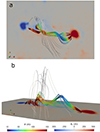 |
Fig. 7. NLFFF extrapolation based on the SDO/HMI vector magnetogram observed at 07:24 UT (panel a shows a view from above, and panel b shows a side view). The colors of lines (black to red) represent the magnetic field strengths, and the colors in the bottom plane (blue to red) show the distribution of Bz. |
Figure 8 displays the dynamic evolution of the coronal magnetic fields. As illustrated in the evolution of the field lines, the flux rope rotated clockwise during its ascent, during which its twist was also released. In particular, the rotation direction is consistent with the helicity rule, namely, the flux rope with positive (negative) helicity generally exhibits clockwise (counter-clockwise) rotation (Green et al. 2007). This reflects the transfer from twist to writhe through the helicity conversion, which also agrees with the prediction of a kink instability. As a result, it is suggested that the trigger of the untwisting motions and filament rise in observations (Figure 3) and MHD simulations might be related to the kink instability. Furthermore, we also computed the twist number distribution in the plane of the flux rope cross-section with the open-source code implemented by Liu et al. (2016). As shown in Figures 8e–h, the twist number initially increased because the rising flux rope induced underlying magnetic reconnection in sheared arcades, which injected twisted fluxes into the preeruptive flux rope. Hereafter, the twist of the flux rope transferred to its writhe the continued ascent, corresponding to the rotation shown in Figures 8a–d. As a result, our MHD modeling roughly reproduces the untwisting motions of the flux rope.
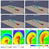 |
Fig. 8. Evolution of the right branch of the filament: Rising phase and untwisting motion with the time evolution from the data-based MHD simulations (panels a–d). Panels (e–h) show the change in Tw along a slice marked by the yellow line in panel (a). An animation of the filament simulation is provided online. |
Figure 9 shows the magnetic topology at t = 1 (a, b, c) and 3 (d, e, f) τ, including the quasi-separatrix-layers (QSLs) and the distribution J/B. QSLs are regions in which the connectivity of the field lines changes drastically, corresponding to areas in which the squashing factor (Q) is larger than 2 (Priest & Démoulin 1995; Demoulin et al. 1996). The flux-rope field lines are very well outlined by QSLs and J/B. Moreover, at t = 1 τ, the magnetic fields of the flux rope are almost tangent to the photosphere and form a bald-patch structure that is tangent to the photosphere. This satisfies the equations as follows (Titov & Démoulin 1999):
 (5)
(5)
 (6)
(6)
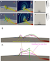 |
Fig. 9. QSLs, electric current density (J/B ), and gas pressure (ρ) distribution of the flux rope cross-section plane at 1 (top panels) and 3 unit times (τ). The yellow lines in panels a–f show the flux rope. The pink and green and yellow and red lines in panels g and h represent flux-rope and sheared-arcade field lines at t = 3 τ, respectively. |
However, with its ascent, a hyperbolic flux tube (HFT) structure is formed below the flux rope. On the one hand, moderate magnetic reconnection occurred in these places, injecting some twisted fluxes into the flux rope, slightly increasing the twist number below the flux rope (Figure 8f), and resulting in bidirectional outflows in observations. This has two effects for the above flux rope (corresponding to the filament in observations). First, the reconnection flows and magnetic tension force resulting from newly formed curved field lines cause the rise of the flux rope. In addition, it is able to increase the lateral Lorentz force acting upon the above flux rope, which is also in favour of its untwisting motion (Kliem et al. 2012; Zhang et al. 2024), corresponding to the twist decrease of the flux rope. On the other hand, the transfer from the bald patch to HFT naturally levitates some chromosphere materials into the solar corona and supplies materials for the filament, increasing the depth of spectra in Figure 6b.
To show the evolution of the field lines in the eruption process, similar to Guo et al. (2025), we traced four typical field lines from the bottom plane of the simulation, as shown in Figures 9g (t = 3 τ) and 9h (t = 8 τ). The yellow and red lines represent sheared arcade field lines at 3 τ, and pink and green lines are twisted flux-rope field lines. However, at t = 3 τ, the sheared arcade field lines become twisted flux-rope field lines due to magnetic reconnection underneath (Figure 9e), corresponding to the twist increase in Figure 8e–g. In contrast, the twist of the preeruptive flux-rope field lines (green and pink lines) decreases as it rises. As a result, our simulation results clearly show the reconnection below the flux rope and the untwisting of flux rope field lines in the eruption process.
5. Conclusion
We studied untwisting motions in a filament and the interaction between its fine threads that produced a B8.4 class on 2 November 2022 at 08:14 UT in AR NOAA 13135. We observed bidirectional outflows both before and after the flare. The former were accompanied by untwisting motions. We display the second bidirectional outflow in the appendix.
The magnetic emergence and cancellation in the middle part of the filament caused it to rise, and the threads interacted with each other at about 07:09 UT. The magnetic reconnection resulted in brightenings in AIA 304 Å and 171 Å that connected the two ends of threads. After the magnetic reconnection, the filament oscillated slightly. Before and after the flare, untwisting motion and bidirectional outflows were again observed by NVST. The threads in the right branch of the filament exhibited highly dynamic characteristics. The threads moved in the opposite direction than before. They became looser, and the twisted structure gradually disappeared. On the other hand, some bright blobs moved from east to west along the spine of the filament observed by AIA 304 Å. The time-distance diagrams also showed bidirectional outflows in different wavelength bands, such as 304 Å of AIA and Hα of NVST and CHASE.
A data-constrained MHD simulation was performed. The initial magnetic field was provided by an NLFFF extrapolation based on a SDO/HMI vector magnetogram. The MHD simulations allowed us to investigate the physical processes behind these observations. The magnetic configuration of this filament corresponds to a combination of sheared arcades (left part) and a twisted flux rope (FR) (right part).
Twist increases as the filament rose due to reconnection of the sheared arcades below. In the sheared arcades below the flux rope, twisted fluxes was injected into the preeruptive flux rope. The FR was tangent to the photosphere and formed a bald patch. As the FR rose, twist could be injected during the magnetic reconnection of the sheared arcades below the FR. The magnetic reconnection favors bilateral outflows in the observations. The twist was studied in detail in the simulations, but it is difficult to derive this evolution in the observations. In the simulations, a stratified hydrostatic atmosphere including the photosphere and corona was adopted. The transformation of the bald patch into HFT due to reconnection as the FR rose implies that more material was included in the FR. This corresponds to the observation of a denser filament with a higher opacity that was observed in the Hα line profiles of CHASE.
With higher-resolution observations, it will certainly be possible to test more physical properties of the FR, such as the helicity. DKIST could provide data like this in the future.
Data availability
The Doppler velocity map sequence and the movies associated to Figs. 1 and 8 are available at https://www.aanda.org
Acknowledgments
The authors are grateful for the anonymous referee’s valuable suggestions. This work is supported by the NSFC grant 12173022, 11790303 and 11973031. J.H.G is supported by the fellowship of China National Postdoctoral Program for Innovative Talents under Grant Number BX20240159. We would like to thank NVST, SDO, SUTRI and CHASE for providing the high resolution data. SDO is a mission of NASA’s Living With a Star Program. The data used in this work were obtained with the NVST in Fuxian Solar Observatory of Yunnan Observatories, CAS. SUTRI is a collaborative project conducted by the National Astronomical Observatories of CAS, Peking University, Tongji University, Xi’an Institute of Optics and Precision Mechanics of CAS and the Innovation Academy for Microsatellites of CAS. CHASE mission is supported by China National Space Administration.
References
- Alexander, C. E., Walsh, R. W., Régnier, S., et al. 2013, ApJ, 775, L32 [NASA ADS] [CrossRef] [Google Scholar]
- Amari, T., Luciani, J. F., Mikic, Z., & Linker, J. 2000, ApJ, 529, L49 [NASA ADS] [CrossRef] [Google Scholar]
- Aulanier, G., & Demoulin, P. 1998, A&A, 329, 1125 [NASA ADS] [Google Scholar]
- Aulanier, G., & Schmieder, B. 2002, A&A, 386, 1106 [NASA ADS] [CrossRef] [EDP Sciences] [Google Scholar]
- Aulanier, G., Demoulin, P., van Driel-Gesztelyi, L., Mein, P., & Deforest, C. 1998, A&A, 335, 309 [NASA ADS] [Google Scholar]
- Aulanier, G., Török, T., Démoulin, P., & DeLuca, E. E. 2010, ApJ, 708, 314 [Google Scholar]
- Babcock, H. W., & Babcock, H. D. 1955, ApJ, 121, 349 [Google Scholar]
- Bai, X., Tian, H., Deng, Y., et al. 2023, Res. Astron. Astrophys., 23, 065014 [CrossRef] [Google Scholar]
- Bi, Y., Jiang, Y., Yang, J., et al. 2015, ApJ, 805, 48 [NASA ADS] [CrossRef] [Google Scholar]
- Chen, P. F., & Shibata, K. 2000, ApJ, 545, 524 [Google Scholar]
- Chen, P. F., Harra, L. K., & Fang, C. 2014, ApJ, 784, 50 [NASA ADS] [CrossRef] [Google Scholar]
- Chen, P.-F., Xu, A.-A., & Ding, M.-D. 2020, Res. Astron. Astrophys., 20, 166 [Google Scholar]
- Chen, Y., Du, G., Zhao, D., et al. 2016, ApJ, 820, L37 [Google Scholar]
- Cheng, X., Ding, M. D., Zhang, J., et al. 2014, ApJ, 789, L35 [NASA ADS] [CrossRef] [Google Scholar]
- Dai, J., Zhang, Q., Qiu, Y., et al. 2023, ApJ, 959, 71 [Google Scholar]
- De Pontieu, B., Title, A. M., Lemen, J. R., et al. 2014, Sol. Phys., 289, 2733 [Google Scholar]
- Demoulin, P., Henoux, J. C., Priest, E. R., & Mandrini, C. H. 1996, A&A, 308, 643 [NASA ADS] [Google Scholar]
- DeVore, C. R., & Antiochos, S. K. 2000, ApJ, 539, 954 [NASA ADS] [CrossRef] [Google Scholar]
- Diercke, A., Kuckein, C., Verma, M., & Denker, C. 2018, A&A, 611, A64 [NASA ADS] [CrossRef] [EDP Sciences] [Google Scholar]
- Feng, L., Inhester, B., & Gan, W. 2015, ApJ, 805, 113 [Google Scholar]
- Goode, P. R., & Cao, W. 2012, in Ground-based and Airborne Telescopes IV, eds. L. M. Stepp, R. Gilmozzi, & H. J. Hall, SPIE Conf. Ser., 8444, 844403 [NASA ADS] [CrossRef] [Google Scholar]
- Green, L. M., Kliem, B., Török, T., van Driel-Gesztelyi, L., & Attrill, G. D. R. 2007, Sol. Phys., 246, 365 [NASA ADS] [CrossRef] [Google Scholar]
- Guo, Y., Schmieder, B., Démoulin, P., et al. 2010, ApJ, 714, 343 [Google Scholar]
- Guo, Y., Xia, C., & Keppens, R. 2016a, ApJ, 828, 83 [NASA ADS] [CrossRef] [Google Scholar]
- Guo, Y., Xia, C., Keppens, R., & Valori, G. 2016b, ApJ, 828, 82 [NASA ADS] [CrossRef] [Google Scholar]
- Guo, Y., Cheng, X., & Ding, M. 2017, Science China Earth Sciences, 60, 1408 [NASA ADS] [CrossRef] [Google Scholar]
- Guo, Y., Xia, C., Keppens, R., Ding, M. D., & Chen, P. F. 2019, ApJ, 870, L21 [NASA ADS] [CrossRef] [Google Scholar]
- Guo, Y., Zhong, Z., Ding, M. D., et al. 2021, ApJ, 919, 39 [NASA ADS] [CrossRef] [Google Scholar]
- Guo, J. H., Qiu, Y., Ni, Y. W., et al. 2023, ApJ, 956, 119 [NASA ADS] [CrossRef] [Google Scholar]
- Guo, J. H., Ni, Y. W., Guo, Y., et al. 2024a, ApJ, 961, 140 [NASA ADS] [CrossRef] [Google Scholar]
- Guo, Y., Guo, J., Ni, Y., et al. 2024b, Rev. Mod. Plasma Phys., 8, 29 [Google Scholar]
- Guo, J., Ni, Y. W., Schmieder, B., et al. 2025, ArXiv e-prints [arXiv:2502.18367] [Google Scholar]
- Hou, Y., Li, T., Yang, S., & Zhang, J. 2019, ApJ, 871, 4 [Google Scholar]
- Hou, Y., Li, C., Li, T., et al. 2023, ApJ, 959, 69 [NASA ADS] [CrossRef] [Google Scholar]
- Hou, Z., Tian, H., Madjarska, M. S., et al. 2024, A&A, 687, A190 [NASA ADS] [CrossRef] [EDP Sciences] [Google Scholar]
- Ji, H., Wang, H., Schmahl, E. J., Moon, Y. J., & Jiang, Y. 2003, ApJ, 595, L135 [NASA ADS] [CrossRef] [Google Scholar]
- Keppens, R., Popescu Braileanu, B., Zhou, Y., et al. 2023, A&A, 673, A66 [NASA ADS] [CrossRef] [EDP Sciences] [Google Scholar]
- Kippenhahn, R., & Schlüter, A. 1957, Z. Astrophys., 43, 36 [Google Scholar]
- Kliem, B., Török, T., & Thompson, W. T. 2012, Sol. Phys., 281, 137 [NASA ADS] [Google Scholar]
- Kumar, P., Karpen, J. T., Yurchyshyn, V., DeVore, C. R., & Antiochos, S. K. 2024, ApJ, 973, 74 [Google Scholar]
- Kuperus, M., & Raadu, M. A. 1974, A&A, 31, 189 [NASA ADS] [Google Scholar]
- Langangen, Ø., Rouppe Voort, L., & Lin, Y. 2008, ApJ, 673, 1201 [NASA ADS] [CrossRef] [Google Scholar]
- Lemen, J. R., Title, A. M., Akin, D. J., et al. 2012, Sol. Phys., 275, 17 [Google Scholar]
- Li, C., Fang, C., Li, Z., et al. 2022a, Sci. China Phys. Mech. Astron., 65, 289602 [NASA ADS] [CrossRef] [Google Scholar]
- Li, L., Peter, H., Chitta, L. P., et al. 2022b, ApJ, 935, 85 [Google Scholar]
- Li, H. T., Cheng, X., Ni, Y. W., et al. 2023, ApJ, 958, L42 [NASA ADS] [CrossRef] [Google Scholar]
- Li, T., & Zhang, J. 2013, ApJ, 778, L29 [Google Scholar]
- Lin, Y., Engvold, O., der Voort, L. R. V., Wiik, J. E., & Berger, T. E., 2005, Sol. Phys., 226, 239 [NASA ADS] [CrossRef] [Google Scholar]
- Lin, Y., Martin, S. F., & Engvold, O. 2008, in Subsurface and Atmospheric Influences on Solar Activity, eds. R. Howe, R. W. Komm, K. S. Balasubramaniam, & G. J. D. Petrie, ASP Conf. Ser., 383, 235 [Google Scholar]
- Liu, R., Gilbert, H. R., Alexander, D., & Su, Y. 2008, ApJ, 680, 1508 [Google Scholar]
- Liu, R., Kliem, B., Török, T., et al. 2012, ApJ, 756, 59 [Google Scholar]
- Liu, Z., Xu, J., Gu, B.-Z., et al. 2014, Res. Astron. Astrophys., 14, 705 [Google Scholar]
- Liu, R., Kliem, B., Titov, V. S., et al. 2016, ApJ, 818, 148 [Google Scholar]
- Liu, J., Zhang, Y., Zheng, Y., Liu, Y., & Chen, J. 2024a, Universe, 10, 42 [Google Scholar]
- Liu, Y., Ruan, G. P., Schmieder, B., et al. 2024b, A&A, 687, A130 [NASA ADS] [CrossRef] [EDP Sciences] [Google Scholar]
- Martin, S. F. 1998, Sol. Phys., 182, 107 [Google Scholar]
- Mei, Z. X., Keppens, R., Roussev, I. I., & Lin, J. 2018, A&A, 609, A2 [Google Scholar]
- November, L. J., & Simon, G. W. 1988, ApJ, 333, 427 [Google Scholar]
- Pesnell, W. D., Thompson, B. J., & Chamberlin, P. C. 2012, Sol. Phys., 275, 3 [Google Scholar]
- Priest, E. 2014, Magnetohydrodynamics of the Sun (Placeholder Publisher) [Google Scholar]
- Priest, E. R., & Démoulin, P. 1995, J. Geophys. Res., 100, 23443 [NASA ADS] [CrossRef] [Google Scholar]
- Ruan, G., Chen, Y., Wang, S., et al. 2014, ApJ, 784, 165 [NASA ADS] [CrossRef] [Google Scholar]
- Ruan, G., Chen, Y., & Wang, H. 2015, ApJ, 812, 120 [NASA ADS] [CrossRef] [Google Scholar]
- Ruan, G., Schmieder, B., Mein, P., et al. 2018, ApJ, 865, 123 [NASA ADS] [CrossRef] [Google Scholar]
- Ruan, G., Jejčič, S., Schmieder, B., et al. 2019a, ApJ, 886, 134 [NASA ADS] [CrossRef] [Google Scholar]
- Ruan, G., Schmieder, B., Masson, S., et al. 2019b, ApJ, 883, 52 [NASA ADS] [CrossRef] [Google Scholar]
- Savage, S. L., McKenzie, D. E., Reeves, K. K., Forbes, T. G., & Longcope, D. W. 2010, ApJ, 722, 329 [NASA ADS] [CrossRef] [Google Scholar]
- Schmieder, B. 2006, J. Astrophys. Astron., 27, 139 [Google Scholar]
- Schmieder, B., & Aulanier, G. 2012, Adv. Space Res., 49, 1598 [NASA ADS] [CrossRef] [Google Scholar]
- Schmieder, B., Malherbe, J. M., & Raadu, M. A. 1985, A&A, 142, 249 [NASA ADS] [Google Scholar]
- Schmieder, B., Tziotziou, K., & Heinzel, P. 2003, A&A, 401, 361 [NASA ADS] [CrossRef] [EDP Sciences] [Google Scholar]
- Schmieder, B., Lin, Y., Heinzel, P., & Schwartz, P. 2004a, Sol. Phys., 221, 297 [Google Scholar]
- Schmieder, B., Mein, N., Deng, Y., et al. 2004b, Sol. Phys., 223, 119 [NASA ADS] [CrossRef] [Google Scholar]
- Schmieder, B., Aulanier, G., Mein, P., & Ariste, A. L. 2006, Sol. Phys., 238, 245 [Google Scholar]
- Schmieder, B., Tian, H., Kucera, T., et al. 2014, A&A, 569, A85 [NASA ADS] [CrossRef] [EDP Sciences] [Google Scholar]
- Schmieder, B., Zuccarello, F. P., Aulanier, G., et al. 2016, Cent. Eur. Astrophys. Bull., 40, 35 [Google Scholar]
- Schmieder, B., Guo, J. H., & Poedts, S. 2024, Rev. Mod. Plasma Phys., 8, 27 [Google Scholar]
- Schou, J., Scherrer, P. H., Bush, R. I., et al. 2012, Sol. Phys., 275, 229 [Google Scholar]
- Shen, Y., Liu, Y., & Su, J. 2012, ApJ, 750, 12 [NASA ADS] [CrossRef] [Google Scholar]
- Song, H. Q., Chen, Y., Zhang, J., et al. 2015, ApJ, 804, L38 [Google Scholar]
- Song, Y. L., Guo, Y., Tian, H., et al. 2018, ApJ, 854, 64 [NASA ADS] [CrossRef] [Google Scholar]
- Song, Y., Su, J., Zhang, Q., et al. 2024, Sol. Phys., 299, 85 [NASA ADS] [CrossRef] [Google Scholar]
- Sterling, A. C., Moore, R. L., Falconer, D. A., & Adams, M. 2015, Nature, 523, 437 [NASA ADS] [CrossRef] [Google Scholar]
- Su, J., Liu, Y., Kurokawa, H., et al. 2007, Sol. Phys., 242, 53 [NASA ADS] [CrossRef] [Google Scholar]
- Su, Y., Veronig, A. M., Holman, G. D., et al. 2013, Nat. Phys., 9, 489 [Google Scholar]
- Su, Y., Gömöry, P., Veronig, A., et al. 2014, ApJ, 785, L2 [NASA ADS] [CrossRef] [Google Scholar]
- Sun, Z., Li, T., Tian, H., et al. 2023, ApJ, 953, 148 [CrossRef] [Google Scholar]
- Titov, V. S., & Démoulin, P. 1999, A&A, 351, 707 [NASA ADS] [Google Scholar]
- Titov, V. S., Downs, C., Mikić, Z., et al. 2018, ApJ, 852, L21 [NASA ADS] [CrossRef] [Google Scholar]
- Wang, H., Cao, W., Liu, C., et al. 2015, Nat. Commun., 6, 7008 [Google Scholar]
- Wang, Y., Ye, P., Zhou, G., et al. 2005, Sol. Phys., 226, 337 [Google Scholar]
- Wang, Y., Zhou, G., Ye, P., Wang, S., & Wang, J. 2006, ApJ, 651, 1245 [NASA ADS] [CrossRef] [Google Scholar]
- Welsch, B. T., DeVore, C. R., & Antiochos, S. K. 2005, ApJ, 634, 1395 [Google Scholar]
- Xia, C., Chen, P. F., Keppens, R., & van Marle, A. J. 2011, ApJ, 737, 27 [NASA ADS] [CrossRef] [Google Scholar]
- Xia, C., Teunissen, J., El Mellah, I., Chané, E., & Keppens, R. 2018, ApJS, 234, 30 [Google Scholar]
- Xu, H., Su, J., Chen, J., et al. 2020, ApJ, 901, 121 [NASA ADS] [CrossRef] [Google Scholar]
- Xue, Z., Yan, X., Cheng, X., et al. 2016, Nat. Commun., 7, 11837 [Google Scholar]
- Xue, Z., Yan, X., Wang, J., et al. 2023, ApJ, 945, 5 [NASA ADS] [CrossRef] [Google Scholar]
- Yan, X., Xue, Z., Cheng, X., et al. 2020, ApJ, 889, 106 [NASA ADS] [CrossRef] [Google Scholar]
- Yan, X., Xue, Z., Jiang, C., et al. 2022, Nat. Commun., 13, 640 [NASA ADS] [CrossRef] [Google Scholar]
- Yan, X. L., Yang, L. H., Xue, Z. K., et al. 2018, ApJ, 853, L18 [Google Scholar]
- Yang, J., Chen, H., Hong, J., Yang, B., & Bi, Y. 2024, ApJ, 964, 7 [NASA ADS] [CrossRef] [Google Scholar]
- Yokoyama, T., & Shibata, K. 1996, PASJ, 48, 353 [Google Scholar]
- Zhang, Q. M., Ning, Z. J., Guo, Y., et al. 2015, ApJ, 805, 4 [Google Scholar]
- Zhang, X. M., Guo, J. H., Guo, Y., Ding, M. D., & Keppens, R. 2024, ApJ, 961, 145 [NASA ADS] [CrossRef] [Google Scholar]
- Zhang, Y., Zhang, Q., Dai, J., Li, D., & Ji, H. 2022, Sol. Phys., 297, 138 [NASA ADS] [CrossRef] [Google Scholar]
- Zheng, R., Chen, Y., Wang, B., Li, G., & Xiang, Y. 2017, ApJ, 840, 3 [NASA ADS] [CrossRef] [Google Scholar]
- Zheng, R., Wang, B., Zhang, L., Chen, Y., & Erdélyi, R. 2022, ApJ, 929, L4 [Google Scholar]
- Zhou, G. P., Zhang, J., Wang, J. X., & Wheatland, M. S. 2017, ApJ, 851, L1 [NASA ADS] [CrossRef] [Google Scholar]
- Zhou, Z., Cheng, X., Zhang, J., et al. 2019, ApJ, 877, L28 [NASA ADS] [CrossRef] [Google Scholar]
- Zhu, C., Liu, R., Alexander, D., & McAteer, R. T. J. 2016, ApJ, 821, L29 [Google Scholar]
- Zirker, J. B., Engvold, O., & Martin, S. F. 1998, Nature, 396, 440 [Google Scholar]
Appendix A: The second bidirectional reconnection outflow
During the flare, flare ribbons intruded into the right branch of the filament, as observed by NVST and AIA. The intrusion destabilized the filament, causing some threads to interact with each other. In the reconstructed Dopplergrams, the intrusion area exhibited significantly stronger blueshift signals than before (see black box in Figure A.1 panels c1–c5). The NVST Hα images (panels a1–a5) reveal that the right branch of the filament became thinner within the black box area. Additionally, flare ribbons segmented the filament threads in the white box region (panels b4–b5). Meanwhile, bidirectional outflows were observed in the right branch, as shown in Figure 4 in 304 Å of AIA and Hα of NVST and CHASE.
 |
Fig. A.1. Evolution of the right branch of the filament, observed by the NVST in the Hα line center (panels (a1)–(a5)) and in 304 Å (panels (b1)–(b5)) between 08:06 UT and 08:20 UT. The reconstructed Dopplergrams in panels (c1)–(c5) show bidirectional outflows after the flare. Black and white box indicate the blueshifted intrusion region in the middle of the right branch of the filament. |
All Figures
|
Fig. 1. Overview of multiwavelength observations in active region AR 13135. Panels (a)–(d) show a map of the magnetic field (HMI) and three intensity maps in 304 Å, 171 Å, and 94 Å from AIA. Panel (e) and panel (f) show Hα observations of CHASE in black and white and NVST in green, respectively. The Hα observation of NVST is the enlarged area of the dashed green box in panel (e). The orange box in the magnetogram (panel a) indicates the region of the right branch of the filament (box R1). The position of the filament is indicated by magenta arrows F in panel b and coronal loops by a yellow arrow in panel d. The associated movie is available online (aa53071-24movie.mp4). |
| In the text | |
|
Fig. 2. Temporal evolution of the middle part of filament at two times (panel a at 07:01:41 UT and panel d at 07:09:26 UT): Zoom of the central NVST image in Hα of Figure 1. The NVST intensity of Hα is shown in green. In panel (d) the blue and orange lines represent the composition of the magnetic flux rope after magnetic reconnection. Panels (b) and (c) show the corresponding brightening in the AIA 304 Åand 171 Å images. Panel (e) shows the corresponding magnetogram. The dashed magenta and yellow lines represent the interacting threads at 07:01:41 UT. The green contour represents the brightening of 304 Å at 07:09:29 UT. The cyan box (R2) represents the area of the calculated magnetic flux shown in Figure 5. In panel (f) we show the time–distance diagram of the slice S1 shown in panel (a). The movement of the threads is indicated by the dashed red line. |
| In the text | |
|
Fig. 3. Untwisting motion evolution of the filament, right branch, observed by the NVST in the Hα line center and by AIA in 304 Å between 07:40 UT and 07:45 UT before the flare. The yellow arrows indicate the threads that untwist and become loose. The observations of NVST are presented in panels (a1)–(a5), in 304 Å in panels (b1)–(b5), reconstructed Dopplergrams in panels (c1)–(c5) (blue and red correspond to blue- and redshift). The curved red arrow in panel (a) represents slice S2, along which the plasma flows. The green arrows in the 304 images indicate the brightening blobs that move west. |
| In the text | |
|
Fig. 4. Time–distance diagrams along the filament (S2 slice shown in Figure 3a) in AIA 304 Å, in NVST Hα, in SUTRI 465 Å, and in CHASE Hα intensity images. They show bidirectional outflows during the filament evolution. The flow velocities are overlaid on the diagrams. The dashed magenta box represents the time range of SUTRI 465 Å, and the dashed blue box shows the time range of CHASE Hα in panel (b). |
| In the text | |
|
Fig. 5. Panel (a) shows the GOES SXR 0.5–4.0 Å and 1–8 Å flux variation and reveals the B8.4 flare. Panels (b) and (d) show the magnetic flux evolution of R1 and R2 (marked by orange and blue boxes in Figures 1 and 2), respectively. The positive (red) and negative (blue) flux are plotted. Panels (c) and (e) show light curves of the EUV channels in R1 and R2 using different colors. The vertical black line represents the peak time of the flare. The green arrow and R4 stand for the time of disturbance of the middle part of the filament. Panel (b) shares a common y-axis for the positive and negative magnetic flux. In panel (d), the values of positive and negative magnetic flux differ significantly, so that the positive values use the left y-axis and the negative values use the right y-axis. R3 covers the time of the untwisting motion of the right branch of the filament before the flare. |
| In the text | |
|
Fig. 6. Observation of CHASE at 08:26:33 UT. The dashed cyan line represents the path along the spine of the filament, and a red point P is on it. Spectrum profiles of point P at different times are shown in panel (b), and the black line represents the line profile of the quiet region. Panel (c) shows the spectrum-time diagram of point P. Panel (d) shows the spectrum along the path at 08:20:36 UT. The vertical black line represents the position of point P. |
| In the text | |
|
Fig. 7. NLFFF extrapolation based on the SDO/HMI vector magnetogram observed at 07:24 UT (panel a shows a view from above, and panel b shows a side view). The colors of lines (black to red) represent the magnetic field strengths, and the colors in the bottom plane (blue to red) show the distribution of Bz. |
| In the text | |
|
Fig. 8. Evolution of the right branch of the filament: Rising phase and untwisting motion with the time evolution from the data-based MHD simulations (panels a–d). Panels (e–h) show the change in Tw along a slice marked by the yellow line in panel (a). An animation of the filament simulation is provided online. |
| In the text | |
|
Fig. 9. QSLs, electric current density (J/B ), and gas pressure (ρ) distribution of the flux rope cross-section plane at 1 (top panels) and 3 unit times (τ). The yellow lines in panels a–f show the flux rope. The pink and green and yellow and red lines in panels g and h represent flux-rope and sheared-arcade field lines at t = 3 τ, respectively. |
| In the text | |
|
Fig. A.1. Evolution of the right branch of the filament, observed by the NVST in the Hα line center (panels (a1)–(a5)) and in 304 Å (panels (b1)–(b5)) between 08:06 UT and 08:20 UT. The reconstructed Dopplergrams in panels (c1)–(c5) show bidirectional outflows after the flare. Black and white box indicate the blueshifted intrusion region in the middle of the right branch of the filament. |
| In the text | |
Current usage metrics show cumulative count of Article Views (full-text article views including HTML views, PDF and ePub downloads, according to the available data) and Abstracts Views on Vision4Press platform.
Data correspond to usage on the plateform after 2015. The current usage metrics is available 48-96 hours after online publication and is updated daily on week days.
Initial download of the metrics may take a while.