| Issue |
A&A
Volume 699, July 2025
|
|
|---|---|---|
| Article Number | A322 | |
| Number of page(s) | 19 | |
| Section | Stellar structure and evolution | |
| DOI | https://doi.org/10.1051/0004-6361/202451962 | |
| Published online | 16 July 2025 | |
Magnetic activity of RS CVn stars based on TESS and LAMOST surveys
1
College of Physics, Guizhou University, 550025 Guiyang, PR China
2
Dept. of Physics and Astronomy and SARA, Butler University, Indianapolis, IN 46208, USA
3
Department of Physics & Astronomy Howard University, Washington, DC 20059, USA
4
College of medicine, Guizhou university of traditional Chinese medicine, Guiyang 550025, P.R. China
⋆ Corresponding author: This email address is being protected from spambots. You need JavaScript enabled to view it.
Received:
23
August
2024
Accepted:
12
May
2025
Abstract
Aims. Understanding flare activity in RS CVn stars is crucial for elucidating their magnetic activity properties. This study aims to conduct a detailed statistical analysis of stellar flare characteristics in RS CVn-type stars using data from the Transiting Exoplanet Survey Satellite (TESS) and the Large Sky Area Multi-Object Fiber Spectroscopic Telescope (LAMOST) surveys.
Methods. We initially identified 80 305 candidates from the International Variable Star Index (VSX) and refined the sample to 1812 RS CVn stars through SIMBAD cross-matching. Using TESS two-minute cadence data, we processed 958 light curves from 246 targets, detecting 1254 flare events among 144 flare stars. By cross-matching with the LAMOST Data Release 10 (DR10) data, we obtain 148 and 482 low-resolution and medium-resolution spectra for 90 and 37 RS CVn-type sources, respectively. With LAMOST data, we calculated and statistically analysed several stellar magnetic activity indicators, such as Hα equivalent width. Combining Gaia survey, TESS Input Catalog, and LAMOST survey data, we investigated relationships between flare parameters and stellar characteristics.
Results. Of the 1,254 observed flare events, more than 89% had durations < 1 h, and more than 90% had amplitudes < 0.01. The flare stars concentrate within temperature (4000–6500 K), mass (< 1 M⊙), and radius (0–5 R⊙) ranges, with 21 stars deriving parameters from their primary components. The flare occurrence percentage is higher for temperatures in the range 3000–4000 K and orbital periods < 10 days. The duration (τ) is related to the energy (E) by the power law τ ∝ E0.3−0.41. The power-law index, α, of the cumulative flare frequency distribution is about 1.22 ± 0.09. We analysed flare rotational phases and find no preference, indicating random occurrence. Medium-resolution spectra reveal asymmetry in the Hα profiles of one source, TIC 46296256, which might be caused by coronal rain, binary motion, or chromospheric condensation.
Key words: stars: activity / stars: flare / stars: statistics
© The Authors 2025
 Open Access article, published by EDP Sciences, under the terms of the Creative Commons Attribution License (https://creativecommons.org/licenses/by/4.0), which permits unrestricted use, distribution, and reproduction in any medium, provided the original work is properly cited.
This article is published in open access under the Subscribe to Open model. This email address is being protected from spambots. You need JavaScript enabled to view it. to support open access publication.
1. Introduction
RS CVn stars are close binary systems in which the hotter component is a subgiant or giant star with a spectral type ranging from F to K, while the cooler component is a dwarf or subgiant with a spectral type from G to M (Biermann & Hall 1976; Martínez et al. 2022). These stars can be classified into three subgroups based on their orbital periods: short period (P ≤ 1 day), classical (1 day ≤ P ≤ 14 days), and long period (P ≥ 14 days) (Lahiri et al. 2023). The term ’RS CVn-type’ refers to these close binary stars, which exhibit significant magnetic activity leading to frequent flare events (Karmakar et al. 2023). Research on flares in RS CVn stars not only enhances our understanding of magnetic activity in these systems but also provides valuable insights into similar phenomena in other stellarenvironments.
Flares are high-energy events characterized by a rapid rise and relatively slow decay of flux in the light curve. They represent the most intense manifestations of the magnetic activity seen in both the Sun and other stars (Karmakar et al. 2022). Recent studies have increasingly utilized photometric light curves from space surveys to investigate flare events (Yang et al. 2023). Cao & Gu (2017) examined optical flares and chromospheric activity variability in the highly active RS CVn star UX Ari. Lahiri et al. (2023) report two superflares and eight moderate flares in the close binary RS CVn-type system DV Psc. Sriram et al. (2023) analysed 11 flares from the RS CVn binary system CF Tucanae using Transiting Exoplanet Survey Satellite (TESS) data. Inoue et al. (2023) conducted simultaneous optical photometric observations with TESS and detect a superflare with an energy release of 7 × 1035 erg. Kunt & Dal (2018) provided results on the physical characteristics and chromospheric activity of the RS CVn binary KIC 7885570, based on Kepler mission data. Tu et al. (2020) studied superflares on solar-type stars using TESS data. Through the Kepler survey, Yang et al. (2017) identify 540 M dwarf stars with flare events. Additionally, RS CVn stars are known for their powerful flares detectable in X-ray observations, with MAXI/GSC detecting a possible X-ray flare from the RS CVn star HR5110 and MAXI/NICER observing a significant X-ray flare from GT Mus (Sasaki et al. 2016, 2019). Kawai et al. (2022) find that during flares, the X-ray and Hα emissions exhibit energy releases ranging from 1036 to 1038 erg and from 1035 to 1037 erg, respectively.
Stellar chromospheric activity is influenced by various factors, including changes in the star’s magnetic field, which affect the subsurface convection zone structure, rotation, and magnetic field regeneration through a self-sustaining dynamo (Hall 2008). RS CVn stars, as chromospherically active stars, show significant chromospheric emission in lines associated with activity, such as Hα (Strassmeier & Fekel 1990; Karmakar et al. 2023). Understanding these mechanisms, which include the Ca H & K lines, Hα emission lines, and UV emission, is crucial for interpreting the coronal emissions of chromospherically active binaries (Sriram et al. 2024). Kunt & Dal (2018) used the Kepler mission data to present the physical characteristics and chromospheric activity of the RS CVn binary KIC 7885570. Bell et al. (2012) found that stars with higher magnetic activity, as quantified by LHα/Lbol, exhibit less variability in Hα emission, measured via the metrics σEWHA/EWHA and structure functions, probably due to the stronger persistent emission that requires larger heating events to produce detectable changes. Cao & Gu (2024) report a potential coronal mass ejection (CME) or chromospheric condensation on the RS CVn-type star II Pegasi (II Peg) using high-resolution spectroscopic observations. Large Sky Area Multi-Object Fiber Spectroscopic Telescope (LAMOST) low-resolution spectroscopic observations, complemented with TESS data, identify 35 candidate compact objects with K/M dwarf companions and reveal orbital periods for 16 sources (Mu et al. 2022). Guo et al. (2024) have discovered eight potential SX Phe stars categorized as ‘δ Scuti stars’ using metal abundance data from LAMOST and Galactic latitude. After detecting an X-ray flare with MAXI/GSC, a large Hα line flare is observed from the RS CVn-type binary UX Ari with the Spectroscopic Chuo University Astronomical Telescope (SCAT) (Nemoto et al. 2024). Therefore, studying RS CVn systems-a unique category of chromospherically active binaries (CABs)-is essential for a comprehensive understanding of their properties.
This study is our third paper exploring flare properties using light curves from the TESS mission, following Yang et al. (2023) and Wang et al. (2024). We used two-minute cadence light-curve data from TESS to analyse flare parameters of RS CVn stars. Additionally, we acquired both low- and medium-resolution spectra from LAMOST to investigate the relationship between Hα emission lines and stellar chromospheric activity. In Section 2, we introduce the TESS and LAMOST data of RS CVn-type stars used in this study. Section 3 discusses the flare parameters of flare stars, including the flare detection procedure. Section 4 focuses on the discussion of chromospheric activity, such as the calculation of Hα equivalent width. Section 5 provides a summary of this study.
2. Data
2.1. TESS data
NASA’s TESS is a groundbreaking mission designed to conduct an all-sky transit survey from space. Its primary goal is to discover thousands of exoplanets by monitoring more than 200 000 bright stars for periodic drops in brightness that indicate the presence of orbiting planets. These data enable detailed research into the masses, sizes, and atmospheres of these exoplanets (Ricker et al. 2015). During its initial two-year mission, TESS observed specific sectors of the sky for 28-day periods, systematically covering almost the entire sky, with the exception of regions near the ecliptic equator (Doyle et al. 2019; Ramsay et al. 2020). For our analysis, we identified 80,305 RS Cvn stars from the International Variable Star Index (Watson et al. 2006). These stars were then cross-matched with the SIMBAD database, focusing on the main types, and resulting in a refined list of RS CVn stars. Using TOPCAT (Taylor 2005), we performed a cross-match with the TESS catalogue based on RA and DEC, obtaining the TESS results. From the TESS results, we downloaded 958 light curves with a two-minute cadence for 246 stars using the Python package lightkurve1. In our research, we use TESS PDC-SAP data.
2.2. LAMOST data
LAMOST, located at Xinglong Station in China, is a unique reflecting Schmidt telescope (Wang et al. 1996; Cui et al. 2012). Since its commissioning in 2012, LAMOST has become renowned for its innovative design that allows it to simultaneously observe thousands of celestial objects through advanced fibre optic technology (Zhao et al. 2012; Luo et al. 2012). Also known as the Guo Shou Jing Telescope, LAMOST has significantly advanced the comprehensive study of stars, galaxies, and various astronomical phenomena (Cui et al. 2012).
In this research, we applied a 2-arcsecond matching criterion to cross-match RS CVn stars–both flaring and non-flaring-from the TESS survey with data from LAMOST Data Release 10 (DR10). This process yields 148 low-resolution spectra and 482 medium-resolution spectra, corresponding to 90 and 37 RS CVn-type sources, respectively, providing valuable data for our analysis.
3. Flare discussion
3.1. Flare detection
3.1.1. Flare detection procedure
A flare is a sudden, intense burst of energy, attracting increasing attention in contemporary research due to its significant impact on stellar environments. Flare events are characterized by a rapid rise and a relatively slower decay in the light curve, making them distinguishable through specific detection methods (Yang et al. 2023).
Two primary methods are used to detect stellar flares. The first involves subtracting the background light curve from the original data, allowing the identification of flare events in the detrended data (Davenport 2016; Lu et al. 2019). The second method leverages machine learning techniques, such as convolutional neural networks (CNNs), to automatically detect flares (Feinstein et al. 2020). Many studies have adapted the first method by applying various techniques and criteria to fit the background light curve (Wu et al. 2015; Van Doorsselaere et al. 2017).
CNNs are particularly effective for analysing time-series data, such as stellar flares, as they automatically learn relevant features from the data. By employing convolutional layers with non-linear activation functions, CNNs can effectively handle non-linear problems and capture intricate patterns within the data. Feinstein et al. (2020) trained CNN models, which they named ‘stella’, using a labelled dataset (Günther et al. 2020). In our work, we used the stella program developed by Feinstein et al. (2020), through which we obtained predicted values for whether the points in the light curves were flares. The predictions were averaged from ten CNN models provided by stella. However, since the CNN models did not handle data for the first or last 100 cadences, we made a secondary development to address this issue and obtain the relevant flare parameters. We summarize this as a method that combines machine learning with traditional flare identification. First, we processed the TESS two-minute cadence light curves using stella with ten trained models. We averaged their predictions to get values for each point on the curves, which was the same as the method used by Feinstein et al. (2020). To refine the flare samples, we combined traditional methods with CNN model predictions. We set constraints to classify candidates into subgroups, regarding points with a CNN prediction greater than 0.5 as flare candidates. We removed points with a prediction over 0.5 to fit the stellar background flux variation and calculated its noise range. We took the average of segment standard deviations as the noise value, σ. We then screened peak points with a prediction greater than 0.5 using a 3σ threshold, marked the maximum point as the flare peak point, and determined the flare boundaries by sliding a five-point window and checking the local standard deviation. After removing flare candidates from the curve, we refitted the background and screened again by the 3σ standard (more details can be seen in Wang, in prep). Using the trained CNN models combined with traditional methods, we predicted flare events in unlabelled data and conducted a statistical analysis to gain insights into the frequency, intensity, and other statistical properties of flares of RS CVn stars.
3.1.2. Flare results
Using the method described above, we can identify flare events in the TESS data. However, it is important to recognize that the program may occasionally flag non-flare events as flare events. To enhance the accuracy of our results, we manually inspected each flagged flare. Figure 1 illustrates the flare detection process using the trained CNN models combined with traditional methods. The top figures show the flares that are considered real. The top left panel depicts the location of a single flare on the light curve, with data points in different colours representing the average prediction values of the CNN models. The top right panel provides the corresponding zoomed-in view of the flare, where red points indicate the confirmed flare and blue points represent the stellar background flux. The middle figures are similar to the top but show the flares considered to be false. The bottom panel shows all the flares identified by the program in the light curve, marked by green vertical lines. Flares identified near gaps, using traditional flare identification methods but not processed by the CNN models (true values with CNN prediction values lower than 0.5), are also marked in the figures. For instance, the first flare on the second segment of the light curve in the panel is one such case. Ultimately, we detect 1254 flare events across 144 of the 246 target stars. These results were extracted from TESS sectors 1-74, and to ensure the accuracy and completeness of this subset we verified the corresponding flares and their locations on the light curves.
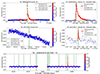 |
Fig. 1. Examples of flare events identified in the light curve by the program. Top panel: Flares classified as genuine, accompanied by a zoomed-in view of the light curve. Middle panel: Flare-like event that was deemed non-genuine and subsequently excluded from the analysis. Bottom panel: All flares flagged by the program, indicated by green vertical lines. The colour of the points on the light curve represents the average prediction values from the 10 CNN models, with the colour bar indicating the corresponding values. Dashed vertical green lines mark the peak times of the identified flares. |
To further our analysis, we cross-matched our TESS sample of RS CVn stars with key databases, including Gaia Data Release 2 (Gaia-DR2) (Gaia Collaboration 2018) and the TESS Input Catalog (Stassun et al. 2019), to obtain additional stellar parameters. Table A.1 lists the parameters of the 1,254 flare events, with the first column showing the TESS ID, the second column the sector, the third and fourth columns the flare amplitude and its error, the fifth column the start time of the flare, the sixth column the time of the flare peak, the seventh column the flare end time, the eighth column the flare duration, and the ninth and tenth columns the bolometric flare energy and its error.
Table A.2 presents a comprehensive list of stellar parameters for the RS CVn stars, including essential details such as effective temperature, mass, and radius. The 20th column of Table A.2 provides the count of flares detected for each target star.
3.2. Flare amplitude and duration
The amplitude and duration of a flare are key parameters for understanding the nature of flare events. We define amplitude as the difference between the flux value of the flare peak (after normalization) and the value corresponding to the background fitting. Flare start time is the time at which the flux first drops below the background value (plus 1.5σ) on the left side of the flare peak. Flare end time is the time at which the flux first drops below the background value (plus 1.5σ) on the right side of the flare peak. Duration is defined as the start time minus the end time. Figure 2 illustrates the distribution of flare amplitude and duration. The left panel of Figure 2 offers a detailed visualization of the varying amplitudes of flares, highlighting their diverse intensities. For all stars in our sample, amplitudes smaller than 0.1 constitute 95% of the total. In addition, we calculated the errors in the amplitude based on the flux errors in the TESS FITS files. Most flare events exhibit low amplitudes (Günther et al. 2020). This finding underscores the advantage of using TESS data to identify smaller flares (Yang et al. 2023). Our results are consistent with previous research, indicating that flare amplitudes typically fall within the small range of 0.001–0.1, particularly between 0.01–0.1 (Walkowicz et al. 2011; Balona 2015; Tu et al. 2021; Yang et al. 2023).
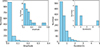 |
Fig. 2. Distribution of flare duration and amplitude. Left panel: Distribution of flare amplitudes. Right panel: Distribution of flare durations across different time intervals. |
In addition to amplitude, duration is another critical parameter for understanding flares. Balona (2015) notes that long-duration flares are more commonly found in stars with low surface gravities. Karmakar (2024) reports one of the longest-duration X-ray flares ever observed, with a duration exceeding 2.3 days. The right panel of Figure 2 provides insight into how the durations of flares are distributed across different time intervals. Our sample reveals that over 98% of the flares have a duration of less than 2 hours, with more than 89% occurring within 1 hour. Didel et al. (2025) analysed three energetic X-ray flares from the active RS CVn binary HR 1099, with flare durations ranging from 2.8 to 4.1 hours. Data from the TESS mission, as reported by Tu et al. (2021), indicate that flare durations on solar-type stars range from 1 to 167 minutes. Walkowicz et al. (2011) identified 373 stellar flares with durations of approximately 3–5 hours using data from the Kepler survey. Our results are consistent with previous research (Yang et al. 2023). The duration and amplitude of flares are also influenced by the exposure time and photometric precision of the telescope (Howard et al. 2022).
3.3. Relationship between the rise and decay times
Flares in light curves exhibit a characteristic rapid rise followed by a slower decay, making the analysis of rise time (Trise) and decay time (Tdecay) within the flare duration essential for understanding flare dynamics. Karmakar (2024), using observations from the Neil Gehrels Swift Observatory, investigated a significant X-ray superflare on the active RS CVn binary system HR 1099, determining that Trise and Tdecay were 14.5 and 41.7 ks, respectively.
We conducted a statistical analysis of Trise and Tdecay for the 1,254 flare events in our sample and present their distributions in Figure 3. The left panel represents the rise time and the right panel represents the decay time. In our sample, Trise ranges from 0 to 100 minutes and Tdecay spans from 5 to 400 minutes. The median values for Trise and Tdecay are approximately6 minutes and 24 minutes, respectively. The minimum values are 1.99 minutes for Trise and 5.99 minutes for Tdecay.
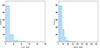 |
Fig. 3. Distribution of rise times and decay times for flare events. Left panel: Distribution of rise times (Trise) for flare events. Right panel: Corresponding decay times (Tdecay). |
For solar-like stars, Yan et al. (2021) report median values of 5.9 minutes for Trise and 22.6 minutes for Tdecay, with mean values of 8.8 minutes and 33.7 minutes, respectively. Our findings show that the mean and median values of Trise are shorter than those of Tdecay, consistent with the results of Yang et al. (2023).
3.4. Flare proportion
We derived the mass, effective temperature, and radius for the flare stars in our sample through cross-matching with data from other missions. Figure 4 shows statistical histograms of the number of flare stars with varying masses, effective temperatures (Teff), and radii, along with their corresponding flare proportions. It is worth noting that only 21 stars have distinguishable primary and secondary star masses and radii. For the known flare stars, we used the parameters of the primary stars. The parameters of these 21 flare stars are listed in Table A.3, while for the remaining flare stars that could not be distinguished, we used the parameters provided by Gaia-DR2 (Gaia Collaboration 2018) or the TESS Input Catalog (Stassun et al. 2019). In the top set of panels, the left panel shows that the masses of the flare stars mainly fall within the 0.6–1 solar mass range, while the middle panel indicates that the effective temperatures of the flare stars are concentrated in the 4500–6000 K range. The right panel shows that the flare stars are concentrated within the 0–2 solar radius range.
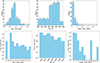 |
Fig. 4. Distribution of flare stars across mass, effective temperature, and radius. Top left panel: Number of flare stars with varying masses. Top middle panel: Number of flare stars with varying effective temperatures (Teff). Top right panel: Distribution of flare stars across different radius ranges. Bottom panels: Corresponding flare proportions. |
We calculated the flare proportion, which is the ratio of the number of stars with flare events to the total number of stars in each effective temperature, mass range, or radius range. This ratio is calculated using
 (1)
(1)
where Nflare-star is the number of stars with flare events and Nstar is the total number of stars within the corresponding temperature or mass range (Yang et al. 2023). From the bottom panels in Figure 4, it can be seen that the flare proportion is higher around a mass of 0.3 M⊙ and Teff of 3000 K to 4500 K, and a radius of 2 solar radii. However, as temperature, mass, and distance change, they affect a star’s quiescent brightness in the TESS band and the flare detection lower limit, thus potentially rendering the data in current figures not always physically meaningful due to the significant impact on the number of detected flares when only amplitude is considered.
3.5. Flare occurrence percentage
The percentage of flare occurrences is calculated using (Walkowicz et al. 2011)
 (2)
(2)
where ∑tflare represents the total flare duration for each star and ∑tstar is the total observation time for each star. Figure 5 presents the distribution of flare occurrence percentages across various ranges of effective temperature and orbital period, using box plots, violin plots overlaid with box-and-whisker plots, and scatter plots to highlight observed trends (Wang et al. 2024). From the left panel of Figure 5, it can be seen that there are more data points in the 4500–6000 K range, indicating higher flare occurrence percentages in this temperature range. The right panel shows that the data points are concentrated in the range of orbital periods shorter than 4 days, and the flare occurrence percentages decrease as the orbital period increases. This pattern underscores a preference for flaring activity among stars with shorter orbital periods and those within a moderate temperature range.
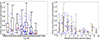 |
Fig. 5. Distribution of flare occurrence percentages across different effective temperature and orbital period ranges. Left panel: Relationship between effective temperature and flare occurrence percentage, with box-and-whisker plots overlaid. Right panel: Relationship between orbital period and flare occurrence percentage, also with violin plots overlaid with box-and-whisker plots. In each panel, blue dots represent the effective temperature or orbital period, along with the corresponding flare occurrence percentage for each star. The horizontal lines of the box plot represent the positions of the quantiles. The upper horizontal line represents the third quartile (3/4), the lower horizontal line represents the first quartile (1/4), and the red line represents the median, while the violin plot shows the distribution shape (in light yellow). |
In Figure 6, we show the relationship between the orbital periods of RS CVn stars (both flare and non-flare) and their effective temperatures, as well as the flare occurrence percentages. The size of the red circles in the figure indicates the percentage of time these stars exhibit flare activity. Notably, stars prone to frequent flaring, especially those with higher flare occurrence rates, tend to cluster in regions where the effective temperature ranges between 4000 and 6000 K, and the orbital periods are shorter than 10 days.
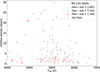 |
Fig. 6. Flare occurrence percentages of all stars. These include both flare stars (red) and non-flare stars (grey), and are shown in the two dimensions of effective temperature and orbital period. The size of the red circles represents the flare occurrence percentage. |
3.6. Flare energy
Flare energy plays a crucial role in evaluating the magnetic activity of stars. In this study, we calculated the bolometric energy of flare events using the method outlined in previous research (refer to Hawley et al. 2014; Petrucci et al. 2024 for detailed star observations in the TESS and Kepler fields):
 (3)
(3)
where Ebol represents the bolometric energy of the flares, ED is the equivalent duration, which is the area under the flare light curve, and LTESS is the quiescent luminosity accounting for the TESS CCD response. The constant, c, valued at 0.19, is a correction factor for the TESS CCD response, representing the fraction of energy released in the TESS band during the flare (Howard & MacGregor 2022; Petrucci et al. 2024; Wang et al. 2024).
As illustrated in the left panel of Figure 7, flare energies for the stars in our sample range from 1032 to 1037 erg, with most concentrated between 1034 and 1035 erg. The right panel of Figure 7 shows the relationship between flare energy and flare occurrence percentage. We employed the Markov chain Monte Carlo (MCMC) method, using ten chains provided by the Python package pymc2, to perform linear fitting (Wang et al. 2024). By overlaying a variety of predictive samples from posterior distributions (shown as grey lines), we determined the mean trend (represented by the red line) by calculating the average fitted slope and its associated uncertainty (Wang et al. 2024). Our analysis reveals that the mean linear slope is negative, indicating that flare energy decreases as the flare occurrence percentage increases. To verify the presence of a declining trend, we conducted trend analysis using three statistical methods: linear regression, Pearson correlation, and the Mann-Kendall trend test. The regression slope is found to be –4.27, the Pearson correlation coefficient is –0.089, and Kendall’s tau is –0.126. All corresponding p-values were less than 0.05, confirming the existence of a potential weak decreasing trend.
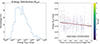 |
Fig. 7. Left panel: Distribution of bolometric flare energy across various energy ranges, with the majority of events concentrated between 1034 to 1035 erg. Right panel: Relationship between flare energy and percentage of flare occurrence. A linear trend fitted using the MCMC method. |
In Figure 8, we further examine the relationships between flare energy and amplitudes (left) and durations (right). Different colours indicate varying point densities and the same MCMC linear fitting approach was applied. The left panel shows that data points mainly cluster where the amplitude is less than 0.025. The right panel indicates that data points are distributed where the duration is less than 1 hour. From Figure 8, it can be seen that all the mean linear slopes are positive, indicating that flare energy increases with the increase in amplitude and duration. To further verify whether an increasing trend exists, we also used the three validation methods mentioned above, and the results confirm the presence of an increasing trend.
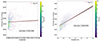 |
Fig. 8. Relationship between amplitude, duration, and energy. Left panel: Relationship between amplitude and flare energy. Right panel: Relationship between duration and flare energy. A linear trend fitted using the MCMC method. |
The upper panel of Figure 9 illustrates the relationship between flare energy and duration across different spectral types. It is observed that for all stellar spectral types there is a general trend where longer flare durations are associated with higher flare energies. The lower panel of Figure 9 shows the results after taking the logarithm of the flare duration, with only main-sequence stars selected. In this panel, the relationship between flare energy and duration becomes simpler and a clear positive correlation emerges. By fitting the flare data for each spectral type, we find that the slopes of the fit lines range between 0.3 and 0.41. We compared our data with solar flare data, and the results, as shown in Figure 10, indicate that our findings are similar to those of solar flares. This suggests that the duration (τ) is related to the energy (E) by the power law τ ∝ E0.3−0.41. These findings are consistent with results from many previous studies on similar topics (Maehara et al. 2015; Namekata et al. 2017).
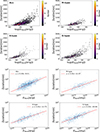 |
Fig. 9. Relationship between flare energy and duration for stars of different spectral types. The colour bar indicates the number density in the upper panels, while the solid red line represents the fitting result in the lower panels. |
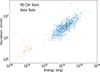 |
Fig. 10. Comparison between the relationship of flare energy and duration for RS CVn stars and for solar data. Solar data from Namekata et al. (2017). |
Typically, the flare frequency distribution (FFD) follows a power-law distribution, expressed as dN/dE ∝ E−α. Power-law indices, α, ranging from 1.1 to 2.2 are reported in numerous studies based on TESS and Kepler data, with the variation dependent on stellar spectral types (Yang et al. 2023; Tu et al. 2021; Yang & Liu 2019; Wang et al. 2024). We selected flare energies between 1033 to 1037 erg to calculate α. The results, presented in Figure 11, indicate that for our sample α is approximately 1.22 ± 0.09, consistent with previous findings. It should be noted that there are certain errors in the calculation of energy. We calculated the errors of the energy by taking into account the errors of TESSMAG and distance (see Table A.2). Since the error is less than one order of magnitude, its impact on our final overall statistical discussion can be neglected.
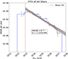 |
Fig. 11. Calculated alpha values for the flare frequency distribution within the energy range of 1033 to 1037 erg using the MCMC method. The green error bars represent the statistical uncertainty, derived as the square root of the total number of flares within each energy range. The dashed vertical red line represents that the fitting energy starts from 1033 ergs. The grey lines represent predictive samples from posterior distributions, while the red line represents the mean trend determined by calculating the average fitted slope and its uncertainty. For the entire sample of flaring stars, the alpha value is found to be approximately 1.22. |
3.7. Flare activity’s dependence on orbital phase
The orbital phase is a key factor in understanding the occurrence of various phenomena, including flares, in RS CVn-type binary systems. The relationship between rotation (or orbital) period and flares has been widely investigated (Wang et al. 2024). Papitto et al. (2018) analysed flares by isolating them from lower-amplitude variations in the K2 light curve, fitting the count rate using a function composed of a quadratic polynomial and Fourier decomposition. Flares were identified by applying Gaussian modelling to the negative portion of the residuals, with bins exceeding 3σ classified as flares. Their study found that the frequency of flare occurrences peaked around an orbital phase of 0.75.
In contrast, Kennedy et al. (2018) examined the K2 light curve to explore the relationship between flare characteristics and orbital phase. Their analysis suggests that the absence of a clear pattern in flare occurrences across orbital phases could be attributed to interdependence among flares, leading to clustering effects on short timescales. Kennedy et al. (2018) emphasize that neighbouring orbital phase bins might not be independent, and that traditional periodicity tests-assuming such independence-might overestimate the significance of any non-uniformity in the flare orbital phase distribution.
The differences between these studies primarily arise from two factors. First, there is a difference in the definition of flares, especially regarding how contiguous data points are segmented into individual flare events (Zhang et al. 2024). Second, Kennedy et al. (2018) considered only the orbital phase of each flare’s peak, while Papitto et al. (2018) considered whether each data point exceeded their iterative significance threshold.
In addition to Kennedy et al. (2018) and Papitto et al. (2018), Doyle et al. (2019) also used TESS data to study the relationship between the number of flares from 149 low-mass stars and their orbital phases. To explore orbital modulation, we studied the relationships between the number of flares, the flare energy, and the phase for 13 eclipsing binary stars. We took the primary minimum as phase 0. The upper panel of Figure 12 shows the distribution of flare energies in different phases, and the lower panel displays the distribution of the number of flares at different phases. We used the  statistic to assess the number of flares, the flare energy, and the rotational phase. The result of the
  statistic shows that there is no relationship between flare number, energy, and rotational phases. In addition, we also performed the Kolmogorov-Smirnov test and the Shapiro-Wilk test, and the results were consistent with the previous findings. Due to the limitation of the sample size, the results need to be verified with a larger sample in the future.
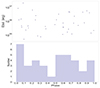 |
Fig. 12. Relationship between flare number, energy, and phase. |
4. Chromospheric activity
4.1. Hα equivalent width calculation
Since the Hα spectral line is crucial in understanding stellar magnetic activity, we calculated the equivalent width (EW) of Hα, denoted as  , using the method provided by Fang et al. (2016) and Fang et al. (2018). The calculation was made using the formula from West et al. (2004),
 (4)
(4)
where Fλ is the intensity of the Hα line and Fc is the intensity of the continuum region on both sides of the Hα line (Su et al. 2024). The error in  was obtained using Monte Carlo simulation. We used a Gaussian distribution to generate random values within the 95% confidence interval, forming a simulated spectrum. Subsequently, we generated 1000 simulated spectra and calculated the
  value of the Hα line in each. The standard deviation of these 1000
  values was used as the final error.
The spectrum utilized the range from 6552.8 to 6572.8 Å, spanning 20 Å for the Hα region. Additionally, two regions of 50 Å each, situated on both sides of the Hα line-6500–6550 Å and 6575–6625 Å -were employed as the continuum regions (West et al. 2004; Xiang et al. 2022). We also calculated the difference between the maximum and minimum  values for each star, denoted as
  . We show the calculation of
  and the distribution of
  in Figure 13. Figure 14 shows the relationship between Hα equivalent width (
 ) and different temperatures, with low resolution on the left and medium resolution on the right. These panels illustrate the EWs of Hα for different temperatures in low resolution and medium resolution spectra from LAMOST. From the panels, we can observe that in low resolution, there is a noticeable decreasing trend in EW as the temperature increases. However, in medium resolution, this trend is less pronounced, showing only a slight downward trend.
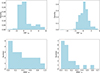 |
Fig. 13. Calculation and distribution of |


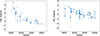 |
Fig. 14. Relationship between Hα equivalent width and effective temperature. Left: For low-resolution spectra. Right: For medium-resolution spectra. All using data from LAMOST. |
4.2. Hα variability
The significant variability of the Hα line has been thoroughly examined by several studies (Lee et al. 2010; Kruse et al. 2010; Bell et al. 2012; Kumar et al. 2023). This variability is essential for investigating stellar chromospheric activity cycles and understanding the relationship between Hα emission and stellar orbital phases. To assess the variability of  , we used repeated observations from LAMOST’s low-resolution and medium-resolution spectra. We focused on stars with two or more observations to evaluate the changes in Hα emission.
To determine whether  exhibits significant variability, we applied the criterion (Long et al. 2021; Mu et al. 2022)
 (5)
(5)
where  and
and  are the maximum and minimum values of the
  line for a star, respectively, and σEW′max and σEW′min are the associated errors (Su et al. 2024). We illustrate examples of RS CVn stars displaying variability in
  in Figure 15, where these variations are clearly depicted. Additionally, the parameters related to chromospheric activity, such as LAMOST Name, OBJECT, OBSID,
  , and Teff are listed in Tables A.4 and A.5 for both low-resolution and medium-resolution spectra.
 |
Fig. 15. Examples of RS CVn stars exhibiting variability in |


4.3. Hα asymmetry
Coronal mass ejections (CMEs) are large-scale expulsions of plasma and magnetic fields from the Sun’s corona, typically occurring during periods of heightened solar activity (Harrison 1996; Chen 2011; Lu et al. 2022). These solar and stellar flares and their associated CMEs can disrupt Earth’s magnetosphere, atmosphere, and communication systems, while also potentially affecting a star’s atmosphere and the habitability of exoplanets (Yang et al. 2023; Fuhrmeister et al. 2018; Koller et al. 2021; Wang et al. 2024). By analysing Hα line blueshifts and asymmetries, Lu et al. (2022) detect three potential stellar CME events. Namekata et al. (2024) report the first discovery of two prominence eruptions on a solar-type star, observed as blueshifted Hα emissions with speeds of 690 and 430 km/s and masses of 1.1 × 10¹⁹ and 3.2 × 10¹⁷. A superflare releasing 7.0 × 1035 erg is detected, with blueshifted Hα excess indicating prominence eruptions reaching velocities of 760–1690 km/s, far exceeding the escape velocity, providing evidence that stellar prominence eruptions can evolve into CMEs. The prominence is found to be a highly massive 9.5 × 10¹⁸ g < M < 1.4 × 10²¹ g (Inoue et al. 2023). Namekata et al. (2021) find that the young solar-type star EK Draconis exhibits a superflare with 2.0 × 1033 erg of energy, accompanied by a blueshifted hydrogen absorption at –510 km/s, suggesting a filament eruption and stellar CME with a filament mass of 1.1 × 10¹⁸ g, ten times larger than the largest solar CMEs. In V374 Peg, three blue-wing enhancements (BWEs) are detected during a flare, with BWE1 and BWE2 suggesting failed eruptions, while BWE3, exceeding the escape velocity at 675 km/s, indicates a complex CME with both ejected and re-ejected material (Vida et al. 2016). In this study, we aimed to detect potential Hα asymmetry in the LAMOST medium-resolution spectra and analyse its underlying causes.
First, we normalized the LAMOST medium-resolution spectra using iSpec and removed the cosmic rays. Using the method outlined by Wang et al. (2024), we first took the average flux of the spectrum as the baseline ( Figure 16) to identify the peak position of the Hα line. Then we calculated the red and blue widths by integrating the regions on both sides of the peak and assessed the symmetry of the Hα profile by comparing the differences between the left and right sides. Finally, we identified several candidates exhibiting asymmetry and then manually examined these cases. Figure 16 displays two examples of Hα profile asymmetries. Through this process, we discover that the Hα profiles in the spectra from two observations of one particular source exhibit asymmetry. This asymmetry is observed in the Hα line of the flaring star TIC 46296256. In Figure 17, the top three panels, from left to right, display the normalized and smoothed Hα profiles, along with the single Gaussian fitting results for the Hα contrast profile of the active spectrum (similar to the method employed by Lu et al. (2022) and Wang et al. (2024)). The contrast profile is obtained through the equation (Lu et al. 2022)
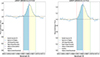 |
Fig. 16. Two examples of Hα profile asymmetries. Left panel: LAMOST J085049.52+121715.8. Right panel: LAMOST J085049.52+121715.6. The dashed red and green lines represent the integration boundaries, the dashed pink and blue lines mark the theoretical and actual peak positions of the Hα profile, and the bright blue and yellow lines highlight the integration areas. The dashed yellow line shows the result of a double Gaussian fit for reference. |
 (6)
(6)
Here, Factive represents the normalized flux of the active spectrum and Fref represents the normalized flux of the reference spectrum. The contrast profile derived from this equation can provide valuable information regarding the spectral differences between the active and the reference at various wavelengths. The layout of the middle three panels mirrors that of the top three panels. In the top three panels, reference spectra are shown in red and green, while in the middle three panels, the reference spectrum is pink. Active spectra are represented in blue across all panels. In the single Gaussian fitting plot, the vacuum wavelength of the Hα line is referenced from van Hoof (2018).
From the Hα profiles in Figure 17, we observe a continuous decrease in the intensity of the Hα emission spectrum, with an enhanced redshift component in the single Gaussian fitting plot, suggesting that the star may be in the decay phase of a flare. The red wing enhancement in the Hα line, often observed in solar or stellar observations, may result from chromospheric condensation or coronal rain-induced broad emission components, or from backward prominence eruption (Lu et al. 2022; Inoue et al. 2023; Cao & Gu 2024). It is difficult to distinguish the causes of the redshift because they are not spatially resolved. One way to identify them is by using Doppler shifts. Chromospheric condensation typically shows downflow velocities of tens of kilometres per second and occurs during the impulsive phase of solar flares, driven by non-thermal heating processes. Coronal rain, formed from dense and cool plasma in the hot corona, falls along post-flare loops to the solar surface with an average velocity of 60–70 km/s, reaching up to 134 km/s during flare events. Solar prominence/filament eruptions usually occur at velocities ranging from 10 to 500 km/s, with detectable backward prominence eruptions being rare and requiring specific spatial conditions (Wu et al. 2022; Cao & Gu 2024). To evaluate the radial velocity, the wavelength of the Gaussian peak was converted into the Doppler velocity (Inoue et al. 2023). We calculate radial velocities of approximately 123.5 km/s and 113.5 km/s for the active spectra relative to the reference spectra in the two sets of plots. Given that the star’s orbital period is 2.69 days (Stassun et al. 2019), we consider that the velocity is not caused by the star’s rotation, and thus we ruled out the possibility of redshift resulting from the rotation. We think the redshift may be caused by coronal rain (Oliver et al. 2016; Lu et al. 2022; Wang et al. 2024). Analysing the TESS light curves, we find that this star is highly active, experiencing several superflares during sectors 44, 45, and 46. The spectral properties of subsequent smaller flares may be influenced by coronal rain from earlier flares, potentially leading to redshifted emission in Hα (Wang et al. 2024). The light curves for sector 46 are presented at the bottom of Figure 17, including a magnified view of the blue region in the sector 46 light curve to support these findings. It should be noted that TESS and LAMOST were not observed simultaneously. Since we can only confirm that it is a binary star system but are unable to distinguish between the primary and secondary stars or determine their parameters, we cannot rule out binary motion as a cause of the observed redshift (Li et al. 2021; Zhang et al. 2022). Additionally, the redshift could also be attributed to chromospheric condensation. Therefore, we propose that the redshift might be caused by coronal rain, binary motion, or chromosphericcondensation.
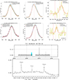 |
Fig. 17. Photometric and spectroscopic images. Top two sets of panels: Normalized (left) and smoothed (middle) Hα profiles, and (right) single Gaussian fitting results for the Hα contrast profile of the active spectrum. The corresponding names from top to bottom are LAMOST J085049.52+121715.6 and J085049.52+121715.8. In the legend, LMJD, S/R, and Hα peak positions are provided, with the peak position of the first spectrum indicated by the dashed red line. The solid yellow line represents the Hα contrast profile and the single Gaussian fitting result is depicted by the solid red line. The dotted vertical red and orange lines indicate the wavelengths of the Hα line at 6562.85 Å and the vacuum wavelength at 6564.61 Å, respectively. Bottom panels: Light curve of TIC 46296256 in sector 46, and a zoom-in view of the blue region in the light curve. |
5. Summary
This study focused on stellar magnetic activity, particularly flare events and Hα lines, using TESS light curves and LAMOST spectra for manually selected RS CVn-type samples. The key findings are as follows:
1. Flare detection and characteristics: We identify 1254 flare events on 144 RS CVn stars using TESS two-minute cadence light curves. Notably, over 89% of these flares have durations shorter than 1 hour, with amplitudes generally ranging between 0.01 and 0.1. The flare stars are primarily concentrated in the ranges of effective temperatures from 4500 to 6000 K, masses below 1 M⊙, and radii less than 5 R⊙.
2. Flare energies and trends: Flare energies range from 1032 to 1037 erg, with a concentration in the 1034 to 1035 erg range. The flare frequency is negatively correlated with flare energy duration. A positive correlation is observed between flare duration, amplitude, and energy. The cumulative flare frequency distribution yields a power-law index of approximately 1.22 ± 0.09. We examined the rotational phase of the flares and find no significant preference for any specific phase, which indicates that the flares occurrandomly.
3. Hα line analysis: Our analysis of LAMOST Hα data indicates a decrease in the Hα EW for flare stars as their effective temperatures increase. Additionally, we identify variability in the Hα equivalent width ( ) in several stars.
4. LAMOST medium-resolution spectra reveal asymmetry in the Hα profiles of two observations of TIC 46296256, which might be caused by coronal rain, binary motion, or chromospheric condensation.
Overall, this study provides a detailed investigation of RS CVn-type stars using TESS and LAMOST data, uncovering important relationships between various stellar parameters and their influence on magnetic activity.
Data availability
Full Tables A.1, A.2, A.4, A.5 are available at the CDS via anonymous ftp to cdsarc.cds.unistra.fr (130.79.128.5) or via https://cdsarc.cds.unistra.fr/viz-bin/cat/J/A+A/699/A322
Acknowledgments
Our research is supported by the NSFC Grant Nos. 12373032. We also thank the fostering project of GuiZhou University with No. 201911, and the CSST project on “stellar activity and late evolutionary stage”. We also acknowledge the science research grants from the China Manned Space Project with No. CMS-CSST-2021-B07 and the SIMBAD database.
References
- Aslan, Z., Derman, E., Akalin, A., et al. 1992, A&A, 257, 580 [Google Scholar]
- Balachandran, S., Carney, B. W., Fry, A. M., et al. 1993, ApJ, 413, 368 [Google Scholar]
- Balona, L. A. 2015, MNRAS, 447, 2714 [Google Scholar]
- Barisevičius, G., Tautvaišienė, G., Berdyugina, S., et al. 2010, Baltic Astron., 19, 157 [Google Scholar]
- Bell, K. J., Hilton, E. J., Davenport, J. R. A., et al. 2012, PASP, 124, 14 [Google Scholar]
- Bickle, T. P., Jalowiczor, P. A., Casewell, S. L., et al. 2022, Res. Notes Am. Astron. Soc., 6, 127 [Google Scholar]
- Biermann, P., & Hall, D. S. 1976, IAU Symp., 73, 381 [Google Scholar]
- Budding, E., Jones, K. L., Slee, O. B., et al. 1999, MNRAS, 305, 966 [Google Scholar]
- Cao, D.-T., & Gu, S.-H. 2017, Res. Astron. Astrophys., 17, 055 [Google Scholar]
- Cao, D., & Gu, S. 2024, ApJ, 963, 13 [Google Scholar]
- Chen, P. F. 2011, Liv. Rev. Sol. Phys., 8, 1 [Google Scholar]
- Cui, X.-Q., Zhao, Y.-H., Chu, Y.-Q., et al. 2012, Res. Astron. Astrophys., 12, 1197 [Google Scholar]
- Davenport, J. R. A. 2016, ApJ, 829, 23 [Google Scholar]
- Didel, S., Pandey, J. C., & Srivastava, A. K. 2025, AJ, 169, 49 [Google Scholar]
- Doyle, L., Ramsay, G., Doyle, J. G., et al. 2019, MNRAS, 489, 437 [NASA ADS] [CrossRef] [Google Scholar]
- Fang, X.-S., Zhao, G., Zhao, J.-K., et al. 2016, MNRAS, 463, 2494 [NASA ADS] [CrossRef] [Google Scholar]
- Fang, X.-S., Zhao, G., Zhao, J.-K., et al. 2018, MNRAS, 476, 908 [NASA ADS] [CrossRef] [Google Scholar]
- Feinstein, A. D., Montet, B. T., Ansdell, M., et al. 2020, AJ, 160, 219 [Google Scholar]
- Fekel, F. C., Browning, J. C., Henry, G. W., et al. 1993, AJ, 105, 2265 [Google Scholar]
- Fekel, F. C., Eitter, J. J., de Medeiros, J.-R., et al. 1998, AJ, 115, 1153 [Google Scholar]
- Franson, K., Bowler, B. P., Zhou, Y., et al. 2023, ApJ, 950, L19 [NASA ADS] [CrossRef] [Google Scholar]
- Fuhrmeister, B., Czesla, S., Schmitt, J. H. M. M., et al. 2018, A&A, 615, A14 [NASA ADS] [CrossRef] [EDP Sciences] [Google Scholar]
- Gaia Collaboration (Babusiaux, C., et al.) 2018, A&A, 616, A10 [NASA ADS] [CrossRef] [EDP Sciences] [Google Scholar]
- Gálvez, M. C., Montes, D., Fernández-Figueroa, M. J., et al. 2002, A&A, 389, 524 [NASA ADS] [CrossRef] [EDP Sciences] [Google Scholar]
- Gálvez, M. C., Montes, D., Fernández-Figueroa, M. J., et al. 2007, A&A, 472, 587 [NASA ADS] [CrossRef] [EDP Sciences] [Google Scholar]
- Günther, M. N., Zhan, Z., Seager, S., et al. 2020, AJ, 159, 60 [Google Scholar]
- Guo, F., Lin, J., Wang, X., et al. 2024, MNRAS, 528, 6997 [Google Scholar]
- Hall, J. C. 2008, Liv. Rev. Sol. Phys., 5, 2 [Google Scholar]
- Harrison, R. A. 1996, Sol. Phys., 166, 441 [NASA ADS] [CrossRef] [Google Scholar]
- Hawley, S. L., Davenport, J. R. A., Kowalski, A. F., et al. 2014, ApJ, 797, 121 [Google Scholar]
- Heckert, P. A., & Ordway, J. I. 1995, AJ, 109, 2169 [NASA ADS] [CrossRef] [Google Scholar]
- Howard, W. S., & MacGregor, M. A. 2022, ApJ, 926, 204 [NASA ADS] [CrossRef] [Google Scholar]
- Howard, W. S., MacGregor, M. A., Osten, R., et al. 2022, ApJ, 938, 103 [NASA ADS] [CrossRef] [Google Scholar]
- Hummel, C. A., Monnier, J. D., Roettenbacher, R. M., et al. 2017, ApJ, 844, 115 [NASA ADS] [CrossRef] [Google Scholar]
- Inoue, S., Maehara, H., Notsu, Y., et al. 2023, ApJ, 948, 9 [Google Scholar]
- Karmakar, S. 2024, Am. Astron. Soc. Meeting Abstr., 243, 447.06 [Google Scholar]
- Karmakar, S., Reale, F., Morenzi, J., et al. 2022, Am. Astron. Soc. Meeting Abstr., 240, 308.02 [Google Scholar]
- Karmakar, S., Naik, S., Pandey, J. C., et al. 2023, MNRAS, 518, 900 [Google Scholar]
- Kawai, H., Tsuboi, Y., Iwakiri, W. B., et al. 2022, PASJ, 74, 477 [NASA ADS] [CrossRef] [Google Scholar]
- Kennedy, M. R., Clark, C. J., Voisin, G., et al. 2018, MNRAS, 477, 1120 [NASA ADS] [CrossRef] [Google Scholar]
- Koller, F., Temmer, M., Preisser, L., et al. 2021, AGU Fall Meeting Abstracts, SH25G-34 [Google Scholar]
- Kruse, E. A., Berger, E., Knapp, G. R., et al. 2010, ApJ, 722, 1352 [Google Scholar]
- Kumar, V., Rajpurohit, A. S., Srivastava, M. K., et al. 2023, MNRAS, 524, 6085 [Google Scholar]
- Kunt, M., & Dal, H. A. 2018, ArXiv e-prints [arXiv:1801.06712] [Google Scholar]
- Lahiri, D., Rani, G. M., & Sriram, K. 2023, Ap&SS, 368, 90 [Google Scholar]
- Lee, K.-G., Berger, E., & Knapp, G. R. 2010, ApJ, 708, 1482 [Google Scholar]
- Li, C., Shi, J., Yan, H., et al. 2021, ApJS, 256, 31 [NASA ADS] [CrossRef] [Google Scholar]
- Long, L., Zhang, L., Bi, S.-L., et al. 2021, ApJS, 253, 51 [NASA ADS] [CrossRef] [Google Scholar]
- Lu, H., Zhang, L., Shi, J., et al. 2019, ApJS, 243, 28 [NASA ADS] [CrossRef] [Google Scholar]
- Lu, H., Tian, H., Zhang, L., et al. 2022, A&A, 663, A140 [NASA ADS] [CrossRef] [EDP Sciences] [Google Scholar]
- Luo, A.-L., Zhang, H.-T., Zhao, Y.-H., et al. 2012, Res. Astron. Astrophys., 12, 1243 [CrossRef] [Google Scholar]
- Maehara, H., Shibayama, T., Notsu, Y., et al. 2015, Earth Planets Space, 67, 59 [NASA ADS] [CrossRef] [Google Scholar]
- Martínez, C. I., Mauas, P. J. D., & Buccino, A. P. 2022, MNRAS, 512, 4835 [CrossRef] [Google Scholar]
- Mu, H.-J., Gu, W.-M., Yi, T., et al. 2022, Sci. Chin. Phys. Mech. Astron., 65, 229711 [Google Scholar]
- Namekata, K., Sakaue, T., Watanabe, K., et al. 2017, ApJ, 851, 91 [Google Scholar]
- Namekata, K., Maehara, H., Honda, S., et al. 2021, Nat. Astron., 6, 241 [Google Scholar]
- Namekata, K., Airapetian, V. S., Petit, P., et al. 2024, ApJ, 961, 23 [Google Scholar]
- Nemoto, N., Urabe, S., Nagashima, N., et al. 2024, ATel., 16423 [Google Scholar]
- Newmark, J. S., Buzasi, D. L., Huenemoerder, D. P., et al. 1990, AJ, 100, 560 [Google Scholar]
- Oláh, K., Kővári, Z., Vida, K., et al. 2012, IAU Symp., 282, 478 [Google Scholar]
- Oliver, R., Soler, R., Terradas, J., et al. 2016, ApJ, 818, 128 [NASA ADS] [CrossRef] [Google Scholar]
- Pandey, J. C., Singh, K. P., Drake, S. A., et al. 2005, AJ, 130, 1231 [Google Scholar]
- Papitto, A., Rea, N., Coti Zelati, F., et al. 2018, ApJ, 858, L12 [NASA ADS] [CrossRef] [Google Scholar]
- Petrucci, R. P., Gómez Maqueo Chew, Y., Jofré, E., et al. 2024, MNRAS, 527, 8290 [Google Scholar]
- Qian, S. B., Zhu, L. Y., He, J. J., et al. 2003, New Astron., 8, 457 [Google Scholar]
- Ramsay, G., Doyle, J. G., & Doyle, L. 2020, MNRAS, 497, 2320 [NASA ADS] [CrossRef] [Google Scholar]
- Ricker, G. R., Winn, J. N., Vanderspek, R., et al. 2015, J. Astron. Teles. Instrum. Syst., 1, 014003 [Google Scholar]
- Sasaki, R., Tsuboi, Y., Nakamura, Y., et al. 2016, ATel., 9144 [Google Scholar]
- Sasaki, R., Tsuboi, Y., Iwakiri, W., et al. 2019, Am. Astron. Soc. Meeting Abstr., 233, 46504 [Google Scholar]
- Savanov, I. S., & Strassmeier, K. G. 2008, Astron. Nachr., 329, 364 [NASA ADS] [CrossRef] [Google Scholar]
- Şenavcı, H. V., Bahar, E., Özavcı, İ., et al. 2020, Contrib. Astron. Obs. Skalnate Pleso, 50, 594 [Google Scholar]
- Sriram, K., Vijaya, A., Lahiri, D., et al. 2023, PASJ, 75, 476 [Google Scholar]
- Sriram, K., Vijaya, A., Lahiri, D., et al. 2024, New Astron., 106, 102127 [Google Scholar]
- Stassun, K. G., Oelkers, R. J., Paegert, M., et al. 2019, AJ, 158, 138 [Google Scholar]
- Strassmeier, K. G., & Fekel, F. C. 1990, A&A, 230, 389 [NASA ADS] [Google Scholar]
- Su, T., Zhang, L.-Y., Long, L., et al. 2024, ApJS, 271, 60 [Google Scholar]
- Tautvaišienÿe, G., Barisevičius, G., Berdyugina, S., et al. 2011, Astron. Nachr., 332, 925 [Google Scholar]
- Taylor, M. B. 2005, ASP Conf. Ser., 347, 29 [Google Scholar]
- Tian, Y. P., Xiang, F. Y., & Tao, X. 2009, Ap&SS, 319, 119 [NASA ADS] [CrossRef] [Google Scholar]
- Tian, Y. P., Ou, Y. K., Zhang, J. F., et al. 2010, PASJ, 62, 515 [Google Scholar]
- Tu, Z.-L., Yang, M., Zhang, Z. J., et al. 2020, ApJ, 890, 46 [NASA ADS] [CrossRef] [Google Scholar]
- Tu, Z.-L., Yang, M., Wang, H.-F., et al. 2021, ApJS, 253, 35 [NASA ADS] [CrossRef] [Google Scholar]
- Van Doorsselaere, T., Shariati, H., & Debosscher, J. 2017, ApJS, 232, 26 [NASA ADS] [CrossRef] [Google Scholar]
- van Hoof, P. A. M. 2018, Galaxies, 6, 63 [NASA ADS] [CrossRef] [Google Scholar]
- Vida, K., Kriskovics, L., Oláh, K., et al. 2016, A&A, 590, A11 [NASA ADS] [CrossRef] [EDP Sciences] [Google Scholar]
- Walkowicz, L. M., Basri, G., Batalha, N., et al. 2011, AJ, 141, 50 [NASA ADS] [CrossRef] [Google Scholar]
- Wang, S.-G., Su, D.-Q., Chu, Y.-Q., et al. 1996, Appl. Opt., 35, 5155 [NASA ADS] [CrossRef] [Google Scholar]
- Wang, Y., Zhang, L., Su, T., et al. 2024, A&A, 686, A164 [NASA ADS] [CrossRef] [EDP Sciences] [Google Scholar]
- Watson, C. L., Henden, A. A., & Price, A. 2006, Soc. Astron. Sci. Ann. Symp., 25, 47 [NASA ADS] [Google Scholar]
- West, A. A., Hawley, S. L., Walkowicz, L. M., et al. 2004, AJ, 128, 426 [NASA ADS] [CrossRef] [Google Scholar]
- Wu, C.-J., Ip, W.-H., & Huang, L.-C. 2015, ApJ, 798, 92 [Google Scholar]
- Wu, Y., Chen, H., Tian, H., et al. 2022, ApJ, 928, 180 [NASA ADS] [CrossRef] [Google Scholar]
- Xiang, Y., Gu, S., & Cao, D. 2022, MNRAS, 514, 4781 [Google Scholar]
- Yan, Y., He, H., Li, C., et al. 2021, MNRAS, 505, L79 [NASA ADS] [CrossRef] [Google Scholar]
- Yang, H., & Liu, J. 2019, ApJS, 241, 29 [NASA ADS] [CrossRef] [Google Scholar]
- Yang, H., Liu, J., Gao, Q., et al. 2017, ApJ, 849, 36 [NASA ADS] [CrossRef] [Google Scholar]
- Yang, Z., Zhang, L., Meng, G., et al. 2023, A&A, 669, A15 [NASA ADS] [CrossRef] [EDP Sciences] [Google Scholar]
- Zhang, B., Jing, Y.-J., Yang, F., et al. 2022, ApJS, 258, 26 [NASA ADS] [CrossRef] [Google Scholar]
- Zhang, L.-Y., Yang, Z., Li, B., et al. 2024, ApJ, 960, 20 [Google Scholar]
- Zhao, G., Zhao, Y.-H., Chu, Y.-Q., et al. 2012, Res. Astron. Astrophys., 12, 723 [CrossRef] [Google Scholar]
Appendix A: Tables
Parameters of 1,254 flare events from TESS survey.
Stellar parameters of TESS objects (including flare stars).
Stellar parameters of 21 flare stars.
Parameters of Low Resolution.
Parameters of Medium Resolution.
All Tables
All Figures
|
Fig. 1. Examples of flare events identified in the light curve by the program. Top panel: Flares classified as genuine, accompanied by a zoomed-in view of the light curve. Middle panel: Flare-like event that was deemed non-genuine and subsequently excluded from the analysis. Bottom panel: All flares flagged by the program, indicated by green vertical lines. The colour of the points on the light curve represents the average prediction values from the 10 CNN models, with the colour bar indicating the corresponding values. Dashed vertical green lines mark the peak times of the identified flares. |
| In the text | |
|
Fig. 2. Distribution of flare duration and amplitude. Left panel: Distribution of flare amplitudes. Right panel: Distribution of flare durations across different time intervals. |
| In the text | |
|
Fig. 3. Distribution of rise times and decay times for flare events. Left panel: Distribution of rise times (Trise) for flare events. Right panel: Corresponding decay times (Tdecay). |
| In the text | |
|
Fig. 4. Distribution of flare stars across mass, effective temperature, and radius. Top left panel: Number of flare stars with varying masses. Top middle panel: Number of flare stars with varying effective temperatures (Teff). Top right panel: Distribution of flare stars across different radius ranges. Bottom panels: Corresponding flare proportions. |
| In the text | |
|
Fig. 5. Distribution of flare occurrence percentages across different effective temperature and orbital period ranges. Left panel: Relationship between effective temperature and flare occurrence percentage, with box-and-whisker plots overlaid. Right panel: Relationship between orbital period and flare occurrence percentage, also with violin plots overlaid with box-and-whisker plots. In each panel, blue dots represent the effective temperature or orbital period, along with the corresponding flare occurrence percentage for each star. The horizontal lines of the box plot represent the positions of the quantiles. The upper horizontal line represents the third quartile (3/4), the lower horizontal line represents the first quartile (1/4), and the red line represents the median, while the violin plot shows the distribution shape (in light yellow). |
| In the text | |
|
Fig. 6. Flare occurrence percentages of all stars. These include both flare stars (red) and non-flare stars (grey), and are shown in the two dimensions of effective temperature and orbital period. The size of the red circles represents the flare occurrence percentage. |
| In the text | |
|
Fig. 7. Left panel: Distribution of bolometric flare energy across various energy ranges, with the majority of events concentrated between 1034 to 1035 erg. Right panel: Relationship between flare energy and percentage of flare occurrence. A linear trend fitted using the MCMC method. |
| In the text | |
|
Fig. 8. Relationship between amplitude, duration, and energy. Left panel: Relationship between amplitude and flare energy. Right panel: Relationship between duration and flare energy. A linear trend fitted using the MCMC method. |
| In the text | |
|
Fig. 9. Relationship between flare energy and duration for stars of different spectral types. The colour bar indicates the number density in the upper panels, while the solid red line represents the fitting result in the lower panels. |
| In the text | |
|
Fig. 10. Comparison between the relationship of flare energy and duration for RS CVn stars and for solar data. Solar data from Namekata et al. (2017). |
| In the text | |
|
Fig. 11. Calculated alpha values for the flare frequency distribution within the energy range of 1033 to 1037 erg using the MCMC method. The green error bars represent the statistical uncertainty, derived as the square root of the total number of flares within each energy range. The dashed vertical red line represents that the fitting energy starts from 1033 ergs. The grey lines represent predictive samples from posterior distributions, while the red line represents the mean trend determined by calculating the average fitted slope and its uncertainty. For the entire sample of flaring stars, the alpha value is found to be approximately 1.22. |
| In the text | |
|
Fig. 12. Relationship between flare number, energy, and phase. |
| In the text | |
|
Fig. 13. Calculation and distribution of |
| In the text | |
|
Fig. 14. Relationship between Hα equivalent width and effective temperature. Left: For low-resolution spectra. Right: For medium-resolution spectra. All using data from LAMOST. |
| In the text | |
|
Fig. 15. Examples of RS CVn stars exhibiting variability in |
| In the text | |
|
Fig. 16. Two examples of Hα profile asymmetries. Left panel: LAMOST J085049.52+121715.8. Right panel: LAMOST J085049.52+121715.6. The dashed red and green lines represent the integration boundaries, the dashed pink and blue lines mark the theoretical and actual peak positions of the Hα profile, and the bright blue and yellow lines highlight the integration areas. The dashed yellow line shows the result of a double Gaussian fit for reference. |
| In the text | |
|
Fig. 17. Photometric and spectroscopic images. Top two sets of panels: Normalized (left) and smoothed (middle) Hα profiles, and (right) single Gaussian fitting results for the Hα contrast profile of the active spectrum. The corresponding names from top to bottom are LAMOST J085049.52+121715.6 and J085049.52+121715.8. In the legend, LMJD, S/R, and Hα peak positions are provided, with the peak position of the first spectrum indicated by the dashed red line. The solid yellow line represents the Hα contrast profile and the single Gaussian fitting result is depicted by the solid red line. The dotted vertical red and orange lines indicate the wavelengths of the Hα line at 6562.85 Å and the vacuum wavelength at 6564.61 Å, respectively. Bottom panels: Light curve of TIC 46296256 in sector 46, and a zoom-in view of the blue region in the light curve. |
| In the text | |
Current usage metrics show cumulative count of Article Views (full-text article views including HTML views, PDF and ePub downloads, according to the available data) and Abstracts Views on Vision4Press platform.
Data correspond to usage on the plateform after 2015. The current usage metrics is available 48-96 hours after online publication and is updated daily on week days.
Initial download of the metrics may take a while.