| Issue |
A&A
Volume 697, May 2025
|
|
|---|---|---|
| Article Number | A201 | |
| Number of page(s) | 18 | |
| Section | Stellar atmospheres | |
| DOI | https://doi.org/10.1051/0004-6361/202553825 | |
| Published online | 23 May 2025 | |
Characterisation of the hyperactive star HD 251108: Spectroscopic monitoring and discovery of optical superflares
1
Thüringer Landessternwarte Tautenburg,
Sternwarte 5,
07778
Tautenburg,
Germany
2
Hamburger Sternwarte, Universität Hamburg,
Gojenbergsweg 112,
21029
Hamburg,
Germany
3
Centro de Astrobiología (CAB), CSIC-INTA,
Camino Bajo del Castillo s/n,
28692
Villanueva de la Cañada (Madrid),
Spain
4
INAF - Osservatorio Astrofisico di Arcetri,
Largo E. Fermi 5,
50125
Firenze,
Italy
★ Corresponding author: bfuhrmeister@tls-tautenburg.de
Received:
20
January
2025
Accepted:
31
March
2025
Giant stars can be magnetically active. A prominent example is HD 251108, which exhibited a giant flare recorded on 7 November 2022 at X-ray and optical wavelengths. We report on a spectroscopic campaign monitoring this star from November 2022 to March 2024, starting with the late phases of the giant flare and accumulating 149 medium-resolution spectra with the TIGRE telescope. HD 251108 shows periodic variations in radial velocity (RV), which we interpret as being caused by the star being part of a binary system, yet the photospheric lines do not show any obvious signs of a second component. Similar periodic changes are found in the effective temperature and in the equivalent widths (EWs) of various chromospheric emission lines with the same period as observed in RV, but with a phase shift. We find these effects could be caused by a plage rotating with the star if the star is rotating synchronously. Since the star shows strong Hα and even He I infrared triplet emission outside the flare, we find it to be hyperactive, even though the star only has moderate lithium abundance of A(Li) = 1.28 dex. We further investigated archival TESS observations of HD 251108 and found that flares with energy releases in excess of 1038 erg at optical wavelengths are not unusual. Finally, considering the November 2022 event in a broader context, we argue that this event likely released more than 1040 erg at optical wavelengths.
Key words: stars: activity / stars: chromospheres / stars: late-type
© The Authors 2025
 Open Access article, published by EDP Sciences, under the terms of the Creative Commons Attribution License (https://creativecommons.org/licenses/by/4.0), which permits unrestricted use, distribution, and reproduction in any medium, provided the original work is properly cited.
This article is published in open access under the Subscribe to Open model. Subscribe to A&A to support open access publication.
1 Introduction
Magnetically induced stellar activity, including flares as perhaps its most vigorous manifestation, has been found for many latetype stars from the pre-main sequence to red giants. While the Sun itself is a star with a rather low level of activity, other stars can sustain much higher activity levels, as measured by activity indicators, such as the widely used Ca II H&K lines (Baliunas et al. 1995). This is especially evident in the case of young stars and close binaries (e.g. BY Dra stars and RS CVn stars), which are are also very active and may produce so-called superflares. Specifically, these are flares with energies that are much higher than 1032 erg, which is the highest historically observed flare energy for solar flares (Emslie et al. 2012).
The magnetic activity of late-type stars is interpreted in the context of the rotation-activity paradigm. Short rotational periods and large rotational velocities are associated with high levels of activity measured in many wavelength bands. As stars age, they lose their angular momentum through magnetic braking, thereby slowing down their rotation. This effect can even be used to determine stellar ages using the method of gyrochronology and we refer to Barnes (2007) for an overview. The Sun has lost most of its initial angular momentum and will become a slow rotator when it starts ascending into the giant branch in five billion years.
Thus, we would generally expect giant stars to exhibit rather low levels of activity. However, some giant stars show high levels of activity, for example, the class of FK Com systems (i.e. very rapidly rotating single giant stars) or RS CVn stars (a class of close binaries with giant star components) are all very active. For a general discussion of the magnetic activity of cool evolved stars, we refer to Schröder et al. (2018).
Following the announcement of the superflare in October 2022 as X-ray transient LXT 221107A, we started a spectral monitoring campaign of HD 251108 using the TIGRE telescope (Schmitt et al. 2014). Our observations went on for two observing seasons, since the star turned out to be remarkable and also puzzling in several ways. We report on our observations here, including the late phases of the superflare. Our paper is structured as follows. In Sect. 2, we present a summary of previous works on this star. We provide detailed information on our spectral data, their reduction, and equivalent width (EW) measurements in Sect. 3. In Sect. 4, we present our results and discuss them in Sect. 5. We present our conclusions in Sect. 6.
2 Previous observations including an X-ray superflare
On the star HD 251108 a superflare event was observed in X-rays on Nov. 7 2022 (Pasham et al. 2022). Günther et al. (2024) presented a thorough discussion of the X-ray properties of this event. In particular, Günther et al. (2024) estimated an X-ray flare energy of 1039 erg (in the 0.5-4.0 keV energy range) and of about 1038 erg in the H α line, thereby placing this flare among the most energetic stellar flares observed up to date. The same authors also infer very high activity levels outside the flare, for example, a persistent quasi-quiescent log (LX / Lbol) ∼−3.0 (utilising data from ROSAT, the XMM-Newton slew-survey, and eROSITA, spanning a timeline of about 30 years) and very high plasma temperatures of 30-50 MK. Hence, the high log (LX / Lbol) is at the saturation limit for main sequence stars, a value that is usually not reached by giant stars, not even in binary systems (Huensch et al. 1996; Gondoin 2007). Only very fast rotating giants such as FK Com may reach it (Gondoin et al. 2002).
HD 251108 is identified with the bright Gaia (Gaia Collaboration 2023) counterpart DR3 3342754943193083392 (mG = 9.600 ± 0.006 mag) at a distance of 505 ± 5 pc (Bailer-Jones et al. 2021). Despite its large distance and its location near the galactic plane, HD 251108 has been assigned a low relative extinction E(B−V) = 0.1 by Paegert et al. (2022); therefore, we neglected extinction in our analysis. Günther et al. (2024) also showed that HD 251108 is evolved and located in the red clump region of the Hertzsprung-Russel-diagram, where in fact many magnetically active giants are found (Hawkins et al. 2017). The effective temperature (Teff) as derived from photometry suggests surface temperatures between 4340 and 5100 K (Xing & Xing 2012; Paegert et al. 2022; Günther et al. 2024; Gaia Collaboration 2023). Some discrepancy is found in radius estimates, where Paegert et al. (2022) listed 12 R⊙ and Günther et al. (2024) found 6-8 R⊙. Previous studies suggested the star to be young and Xing & Xing (2012) measured an EW of H α=−1.54 Å and EW(Li 6707) = 115 m Å, which translates to an abundance of A(Li) = 1.68 dex according to their analysis, making the star lithium-rich.
3 New observations and EW calculation
3.1 TIGRE
Between November 2022 and March 2024, we obtained 149 spectra of HD 251108 with the TIGRE telescope, a robotic telescope located at the La Luz Observatory near Guanajuato (Mexico). TIGRE is equipped with the two channel fibrefed Échelle spectrograph HEROS (Heidelberg Extended Range Optical Spectrograph), which covers the wavelength range from 3738 Å to 8838 Å with a small gap around 5750 Å. This makes it well suited for activity studies, since it covers some strong lines that are known to be chromospheric activity indicators. Its resolution of about 20000 also allows us to resolve the line shapes; a detailed description of the properties of TIGRE and HEROS can be found in Schmitt et al. (2014) and González-Pérez et al. (2022). The TIGRE spectra were reduced with the fully automatic pipeline v3.1, as described by Mittag et al. (2010, 2016) and Hempelmann et al. (2016).
3.2 CARMENES
An additional spectrum was taken with the CARMENES spectrograph, installed at the 3.5-m Calar Alto telescope. CARMENES covers the wavelength range from 5200 to 9600 Å in the visual channel (VIS) and from 9600 to 17100 Å in the near-infrared channel (NIR). The instrument provides a spectral resolution of about 94600 in VIS and 80400 in NIR. A detailed description of CARMENES can be found in Quirrenbach et al. (2020). The spectrum was reduced using the standard CARMENES reduction pipeline (Zechmeister et al. 2014; Caballero et al. 2016).
Parameters of the EW calculation.
3.3 TESS
In their analysis of the NICER X-ray data of HD 251108, Günther et al. (2024) also present observations of HD 251108 taken with the TESS satellite Ricker et al. (2015) in sectors 6, 33, and 43-45. Here, we present additional observations taken in the sectors 71 and 72 and identify two optical superflares on HD 251108.
To obtain the light curves, we downloaded 50x50 pixel-sized cutouts of the TESS full-frame images (FFI) centred on the position of HD 251108 from the MAST archive using the TESScut tool1. We then screened the data for good quality measurements (setting the flag QUALITY as zero). We averaged the pixel fluxes within 3 × 3 pixel apertures centred on the object and subtracted the background, estimated as the median pixel flux in the entire 50 × 50 pixel image.
Times are given as so-called TESS Julian dates, given by JD-2457000. The barycentre correction is given by BTJD-TJD; thus, the time system is TDB, but at the position of the TESS spacecraft; the rates are actually pixel rates, however, we later calibrated the light curves with an assumed bolometric flux for HD 251108.
3.4 Computation of EWs
For several chromospheric lines, we computed the EWs to assess the activity state of HD 251108 in each spectrum. From the EW calculation, we list the central wavelength, the width of the integration band, and the two reference bands in Table 1. The width of the line band was chosen to fully cover the very broad lines, while the reference bands were chosen not to cover photospheric lines. The EW was calculated using the expression
 (1)
where F is the flux density in the line band, F0 is the mean flux density in the one or two reference intervals (representing the continuum), and λ denotes the wavelength. We did not use the Ca II H line. We did so because the continuum is quite noisy in this wavelength range, which limits the meaning of these measurements, and we used only the Ca II K line for comparison to the other lines.
(1)
where F is the flux density in the line band, F0 is the mean flux density in the one or two reference intervals (representing the continuum), and λ denotes the wavelength. We did not use the Ca II H line. We did so because the continuum is quite noisy in this wavelength range, which limits the meaning of these measurements, and we used only the Ca II K line for comparison to the other lines.
4 Results
In the following, we present our results for stellar parameter determination, RV measurements, TESS observations of superflares, and variability of stellar activity. Our Teff, RV, and EW(H α) measurements for each spectrum can be found in Table A, published online (cf. Sect. 6).
Wavelength ranges used for the estimation of stellar parameters.
4.1 Estimation of stellar parameters
4.1.1 Stellar parameter from the TIGRE spectra
Since the stellar parameters of HD 251108 are not well known, we determined them using our TIGRE and CARMENES spectra as well as PHOENIX (Hauschildt et al. 1999) model spectra from their latest model library (Husser et al. 2013). In an alternative approach, we also applied MOOG to an averaged TIGRE spectrum and to the CARMENES spectrum. This was done in the context of our lithium abundance analysis, as described in Sect. 4.3. Here, we concentrate on the comparison to the PHOENIX spectra, where we determined the effective temperature (Teff), surface gravity (log g), and rotational velocity (v sin (i)), assuming solar metallicity, since the given grid size in [M / H] = 0.5 in the model library is too large to obtain a reliable result for HD 251108. For Teff we used a sub-grid covering the range from 3900 to 5500 K (in 100 K steps) and log g from 2.0 to 4.5 (in 0.5 dex steps), and for the v sin (i) estimation, we used a range from 1 to 29 km / s in 1 km / s steps. Furthermore, we chose to compare spectra and model for our fit in certain wavelength ranges listed in Table 2, which we also used to compute the standard deviation of the residuals between both spectra. The minimal standard deviations by the given parameter (Teff, log g, and v sin (i)) for each spectrum are fitted with a parabola to find the minimum of the standard deviation distribution and hence the best fit value for each parameter. The results of our stellar parameter measurements for each TIGRE spectrum are shown in the three panels in Fig. 1. Finally, we calculated the median values of the individual parameters for the two observing seasons and list them in Table 3.
Figure 1 (upper panel) shows that the effective temperature, Teff, does not seem to be constant; rather, it varies between 4450 and 4650 K in a periodic fashion. To estimate the period, we used the generalised Lomb-Scargle (GLS) method (Ferraz-Mello 1981; Zechmeister & Kürster 2009) and found a period of 21.3 days. This is in agreement with the findings of Günther et al. (2024), who found a variation in photometric colour using ASAS-SN photometry data with the same period. This period is also the period of brightness variations, which Günther et al. (2024) modeled using a spot model, leading to 4450 ± 50 K for the bright state and 4100 ± 100 K for the faint state with an estimated filling factor of 0.6 ± 0.1 for the 'spot' (i.e. the cooler and darker area). While we found systematically higher Teff values, our temperature variation is lower with only about 100-200 K. This discrepancy and the high spot filling factor indicate that each spectrum should be better fitted with a two-temperature model (see also Sect. 4.1.2). Unfortunately, the resolution of the TIGRE spectra is relatively low, which makes a unique two temperature fit impossible.
Moreover, log g can (as seen in Fig. 1) vary between 3.0 and 3.5 and shows a slight decline. Also there is a statistically significant difference between the median values obtained for the observing season 2022/2023 and 2023/2024. We find that log g correlates to Teff with a Pearson's r = 0.64 and p = 10−14. Accordingly, there is also some periodicity found in the log g values but with a less significant false alarm probability. This may be caused by stellar oscillates (see for further discussion Sect. 5.2) but also by line deformations caused by spots. They are too weak to be directly detected in the medium resolution TIGRE spectra, but using nine Fe I lines (at positions of 6024.06, 6065.48, 6219.28, 6393.6, 6546.24, 6677.99, 6750.15, 7445.75, and 7568.90 Å) to build an average line profile over all spectra and then subtracting an averaged line profile of each observation (and normalising with the overall mean profile) allows us to detect periodic deviations from the line profile as we show in Fig. 2. This can also be the reason for the trend seen in v sin (i) in the TIGRE spectra. Such quasi-periodic line profile variation can be caused by rotating star spots (and their possible evolution).
Furthermore, we find a difference between the median v sin (i) values of the two observing seasons, which have a T-test p -value of 1.4 × 10⁻⁷ of being constant. Nevertheless, there is no significant correlation (Pearson“s p > 0.03) between v sin (i) and log g or Teff. Since we deem the v sin (i) variations not to be physical, we recalculated Teff and log g for a fixed value of v sin (i) = 17 km / s, but found only very small deviations, which did not change the overall pattern of a decline in log g and a periodic variation in Teff.
 |
Fig. 1 Best-fitting stellar parameters versus time. The black dots depict the parameters obtained from the TIGRE spectra and the red diamond the parameters obtained from the CARMENES spectrum. |
Results of stellar parameters estimation with PHOENIX and spectral synthesis.
 |
Fig. 2 Line profile evolution of an average line profile of nine Fe I lines. The colour scale gives the difference of the normalised flux density to the (also normalised) mean spectrum. The black line marks our RV determination from Sect. 4.2 with its mean shifted to zero RV for display convenience. |
4.1.2 Stellar parameters from the CARMENES spectrum
Applying the same method for determination of the stellar parameters to the CARMENES spectrum with its higher spectral resolution yields parameters of Teff = 4593 ± 5 K, log g = 3.44 ± 0.03, and v sin (i) = 16.6 ± 0.1 km/s. These values are in very good agreement with the values obtained from the lower resolution TIGRE spectra taken around that time, as can be seen in Fig. 1.
During the parameter determinations, we also noted a slight asymmetry in the CARMENES spectrum in many of the strong photospheric lines. We show an example of this asymmetry, manifested as a broadening feature on the red side of the line, in Fig. 3. This bump in the line shape may be caused by a variety of phenomena like infalling material, a severe line blend, or by the star spot. Since we consider the deformation to be the same as the hardly noticable asymmetry in the lower resolution TIGRE spectra from Fig. 2, we can exclude infalling material. We regard the spot being most probable since the CARMENES spectrum is taken by chance at a very low relative RV of the system, so that possible line blends are expected at the centre of the line, not in the wing (cf. Sect. 4.2). We neglected the asymmetry in the parameter determination. Since the feature influences the width of the line, we note that our log g and v sin (i) estimates may be affected and should be considered as upper limits; also, the effective temperature Teff would be lower in case of lower log g.
Although our purely statistical errors for the stellar parameters are small, the error budget may be dominated by systematic errors, since the wealth of weak lines may dominate the results. As an example of a strong line suggesting a lower Teff and log g, we overplot the CARMENES spectrum in Fig. 3 with a PHOENIX model with Teff = 4400 K and log g = 2.5, which yields a better description of the line core, while the wings are better described by Teff = 4600 K and log g = 3.5. We therefore cannot rule out lower values, namely, Teff = 4400 K and log g = 2.5, which would be far more appropriate for a red clump giant. Moreover, these values are in full agreement with the photometric measurements by Günther et al. (2024) for Teff = 4460 K for this RV phase.
 |
Fig. 3 Top: asymmetry of the photospheric Ca I line at 6440.8 Å. We show the CARMENES spectrum in black. The asymmetry can be noted as weak bump at about 6441.2 Å. For comparison we also show a PHOENIX model spectrum with Teff = 4600 K and log g = 3.5 in red and with Teff = 4400 K and log g = 2.5 in blue. Bottom: zoom on the Ca I line at 6464.36 Å. The asymmetry there is even more severe and suggests that the stellar spectrum should be fitted with a two temperature model. |
4.2 RV variations
We performed RV measurements for each TIGRE spectrum using the best spectral model for the two observing seasons from Table 2 and applying the TIGRE standard RV estimation, described in detail by Mittag et al. (2018). The resulting RV values are plotted in Fig. 4 and show a strong periodic variation. To determine the period, we again performed a GLS analysis (Ferraz-Mello 1981; Zechmeister & Kürster 2009) and the corresponding periodogram is shown in Fig. 4 with a main peak at 21.1 days; the secondary peaks around the main peak are caused by the large data gap between the two observing seasons.
For the further analysis, we performed a Keplerian fit to the RV data and the results are listed in Table 4. The resulting best fit curve is shown in red in Fig. 4a. To check the accuracy of the fit, we calculated the residuals and plotted them in Fig. 4b. The large systematic deviations indicate that the fit has systematic deficits. Thus, to quantify the goodness of fit, we computed the standard deviation and the reduced  and obtained a standard deviation of 0.64 km / s for the residuals and
  , also showing that this fit does not describe the data well.
A phase-folded representation of the RV data (shown in Fig. 4d) shows a difference in amplitude and shape for the two observing seasons: while the amplitude declines from observing seasons 2022/2023 to 2023/2024, the maximum and minimum also appear to be slightly shifted to higher or lower phase values, respectively. Both is hard to explain in the context of a binary but easy to understand in the context of (evolving) star spots or a combination of both scenarios. Since Figure 4b shows periodic residuals after subtracting the sine-fit, these should cause the differences in amplitude and shape and we think these to be the imprint of the large spot. We therefore show them phase-folded in Fig. 5, which shows clear spot migration and evolution from one season to the other, but also variations within the seasons, especially in the second one. We further discuss this in Sect. 5.2.
With the amplitude and period of the RV curve we calculated the lower limit of the mass of the secondary star using the binary mass function, f :
 (2)
(2)
Here, M1 and M2 are the mass of the primary and secondary, respectively, with Porb being the orbital period, K the amplitude of the RV curve, i the inclination, and G the gravitational constant. Since f = 3 × 1030 g in our case, M1 ≫ M2 which leads to  . Günther et al. (2024) estimated the mass of the primary to be about 1 M⊙, which would lead to a lower limit of M2 = 0.1 M⊙, since the inclination, i, is unknown. With the companion being a mid-type (or early-type for moderate inclinations) M dwarf, we do not expect to be able to observe an imprint of its spectrum in our observed (combined) spectrum.
 |
Fig. 4 TIGRE RV data: panel a shows the obtained RV values of the individual spectra (black dots) versus time and the red solid line depicts the RV fit. Panel b shows the residuals. Panel c the periodogram of the GLS analysis. Panel d the phased folded RV data, with the data from observing season 2022/2023 shown as black dots and from 2023/2024 as magenta dots, while the red solid line represents the RV fit in phase. |
Results of the RV estimation.
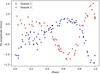 |
Fig. 5 RV residuals to sinusoidal fit like in Fig. 4b, but phase-folded. We can notice strong spot migration and evolution from one season to the other. Also, there is more evolution in the second season. |
4.3 Lithium abundance
We detected the Li I 6707 Å line in the CARMENES and the TIGRE spectra with an EW (Li 6707 Å) = 0.157 Å in the CARMENES spectrum, which includes some contribution by an Fe I line at 6707.44 Å, which cannot be deblended. We do not see any obvious changes in the Li 6707 Å line in the TIGRE spectra, but there may be small deformations in the line shape (as seen in Figs. 2 and 3), since in the CARMENES spectrum also a very weak deviation in the Li 6707 Å line can be noted. However, considering the line broadening by the rotation and the blending with the nearby Fe I line it is hard to detect any possible asymmetry in a single line. Keeping this in mind we added all TIGRE spectra to gain higher signal to noise (S/N) resulting in S/N=223 compared to S / N=42 for the CARMENES spectrum. With this combined TIGRE spectrum and with the CARMENES spectrum, we performed spectral synthesis using the code MOOG (version 2019)2 (Sneden 1973) and MARCS model atmospheres to determine the Li abundance under local thermal equilibrium (LTE) conditions. For consistency, we also determined the stellar parameters (Teff, log g, iron metallicity [Fe / H], and v sin (i)) using the spectral synthesis technique with FASMA3, which is also based on MOOG and whose methodology is described in Tsantaki et al. (2023a).
We determined the stellar parameters first with the averaged TIGRE spectrum and show them in Table 3 and in Fig. 6. This gives a Teff lower by about 200 K than the median Teff determined with PHOENIX. We also used the higher resolution CARMENES spectrum, which is unfortunately relatively noisy at blue wavelengths. We obtained a Teff, which is about 150 K higher than the temperature found using PHOENIX and our selected wavelength ranges from Table 2. When omitting the noisier blue wavelength range, we instead find stellar parameters well in agreement with the TIGRE averaged spectrum. These stellar parameters can be found in Table 1. The difference in Teff may either be caused by the noise in the blue range or by a higher influence of the hotter stellar surface component in this range. This again demonstrates the difficulties in obtaining the stellar parameters and suggests again that finally a two temperature model is needed.
We derived lithium abundances from both the CARMENES and TIGRE spectra using the spectral synthesis technique as in Tsantaki et al. (2023b) using the respective stellar parameters we derived above. We obtained lithium abundance of A(Li) = 1.00 ± 0.06 dex for CARMENES and for the averaged TIGRE spectrum, we find A(Li) = 1.02 ± 0.06 dex, which are in agreement with each other. Lithium abundances are affected by non-LTE (NLTE) effects. We used the tabulated NLTE corrections by Lind et al. (2009) and after interpolating the grid of NLTE corrections, we find A(Li) = 1.26 and 1.28 dex for the CARMENES and TIGRE spectrum, respectively. Xing & Xing (2012) found a somewhat higher A(Li) = 1.68 ± 0.2 dex. However, they considered the star to be young and used a log g grid ranging from 3.0 to 4.5 without stating the actual value used for the star. Furthermore, Xing & Xing (2012) seem to deblend the Li from the neighboring Fe I line, but given the rotational velocity of HD 251108 this may contribute an additional error for this star in their lithium abundance.
We conclude that HD 251108 is not a canonical lithium-rich star (defined by A(Li)>1.5 dex). Nevertheless, in open clusters, there are examples of stars with such lithium abundance that are clearly enhanced with respect to other members at similar evolutionary stage (Tsantaki et al. 2023b). Also Kumar et al. (2020) state that compared to theoretically expected lithium abundance or compared to the abundance at the red giant branch tip (as the previous evolution state) all red clump giant stars are lithium rich. But regardless of the exact value of the threshold of lithium rich giant stars, the lithium abundance of HD 251108 is in the range where enhanced levels of activity and a correlation of activity indicators to RV have been observed (Rolo et al. 2024).
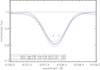 |
Fig. 6 Fit of the Li I 6707 Å line using the TIGRE mean spectrum. The lithium abundance is quite robust against changes in log g as can be seen when comparing the value obtained using the spectroscopically determined log g = 2.85 with the one using the trigonometrically determined log g = 2.43. |
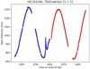 |
Fig. 7 TESS FFI light curve for sector 71 (blue data points) and sector 72 (red data points). |
4.4 Observations of superflares
We show the TESS light curves of sectors 71 and 72 in Fig. 7. Overall about two and a half cycles are covered by the adjacent TESS observations. In the light curve one notices two major flares, one at flux peak (i.e. spot minimum) near TJD 3245, in the following referred to as flare I, and another even larger flare near TJD 3255 and flux minimum (i.e. near spot maximum), in the following referred to as flare II. Both can also be identified in Fig. 10 (at time~2023.82 and 2023.84 years). Already in sector 33 at TJD 2204 a similar large flare was observed and already shown but not discussed in detail by Günther et al. (2024). This flare III has a special morphology, which suggests two overlapping but maybe independent flares, which is the reason why we discuss it here in more detail. We do not discuss all other (smaller) flares, which are visible in the light curve.
4.4.1 Flare light curve determination
To determine the flux attributable to the flaring emission, we need to subtract the photospheric background emission. The three flares all have rather long durations with enhanced emission notable for more than one day, during which the background flux varies, and these variations must be properly accounted for. Our procedure for this is illustrated in Fig. 8 for flare I. In the upper panel of Fig. 8, we plot the actual data (blue points), as well as the data from the subsequent cycle of HD 251188, shifted by one period backwards and raised by 5.5 flux units (green points); the red solid curve shows a polynomial fit to the latter data. Since the photospheric background has not substantially changed in one period, we subtracted the modelled background (red solid curve) from the data (blue points) and obtain the net flare emission shown in the lower panel of Fig. 8. We recognise a sharp increase in count rate that lasts, however, almost half a day, followed by an exponential decay over a little less than two days before the flare signal is lost in the noise.
The light curve analysis of flare II is carried out in a similar fashion as that of flare I. As reference data, we use here the data from the previous cycle of HD 251188 shifted by one period forwards (green points), but without vertical shifts. In the net flare light curve, we again notices a sharp increase in count rate that occurs, however, in two steps. An exponential decay with a duration of more than one day follows. Then one or several reheating events follow before the flare emission ceases.
For flare III, we used as our reference, the data from the next cycle of HD 251188 shifted by one period backwards (green points). Flare III has a more complicated structure, since it looks like two independent flares that partially overlap. The decay times of these two events are very similar, yet the second flare is more powerful.
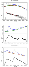 |
Fig. 8 Flare light curves of the three flares: original data (blue points), reference data (light curve shifted backwards and forwards by one period; see text for details; green points) together with polynomial fit (solid red line), and net flare light curve (black points). |
4.4.2 Flare energetics
In this section, we explain how we derived the basic energetics of the flares shown in Fig. 8. To this end, we need to convert the observed TESS rates into physical fluxes and luminosities. Gaia Collaboration (2023) present physical parameter estimates of HD 251108 and from their corner plots we estimate R* ≈ 10.7 R⊙ and Teff ≈ 5100 K. This value is higher than the effective temperatures derived from high-resolution spectroscopy, however, the pair of R* and Teff is consistent with Gaia photometry and distance of HD 251108. With the Gaia values one finds Lb o l ≈ 70 Lb o l, ⊙ and this is the value we assume for our subsequent energy calculations.
As is obvious from Fig. 7, the TESS flux is modulated by almost 30 %. As shown by Günther et al. (2024), there are also color changes associated with these modulations in the sense that the star becomes redder when it is fainter, consistent with the idea that cooler star spots are responsible for the modulations. Since TESS does not provide color information, the TESS data do not offer diagnostic means to take these effects into account. Furthermore, the flaring plasma is likely to have a possibly considerably increased temperature in comparison to the non-flaring atmosphere and again we have no means to diagnose these effects in a quantitative manner; for a more detailed discussion of these issues we refer to Schmitt et al. (2021). Thus, we ignored all these effects and use the same rate-to-flux conversion for all stellar emission components. To be specific, we assumed the mean rate level of HD 2151108, estimated to be at 1025 s−1 from Fig. 7, to correspond to a luminosity of 2 × 1035 erg / s.
To obtain the total flare energy including the reheating events, we numerically integrate the observed net flare light curves. The quoted decay times refer to the initial exponential decay observed in the flare light curves. To compute a characteristic scale of the flaring area we need to assume some (unknown) temperature of the flaring plasma; we therefore choose temperatures of 8000 K and 15000 K, which may encompass the true temperature range (Kowalski 2024). The characteristic sizes were derived by assuming that the flaring emission is produced as blackbody emission with the specified temperature in a circular region.
Flare III is clearly somewhat more complicated. However, it may also be the sum of two actually unrelated events dubbed Flare IIIa and FlareIIIb in the following. The decay times of the two flares are very similar, yet FlareIIIb contributes two thirds of the total energy; the flare areas were computed assuming independent events. All of the derived numbers are listed in Table 5.
Physical flare parameters of observed TESS flares.
4.4.3 ASAS flare energetics
Using an All-Sky Automated Survey for Supernovae (ASAS) light curve (shown by Günther et al. (2024) in their Fig. 8), we can accomplish a similar flare energy estimate like for the TESS data for the large flare on 7 Nov. 2022. An inspection of the available ASAS data shows that on 7 Nov. 2022 8:55 UT three measurements were taken within a few minutes, which show a flux increase (in the g band) of about a factor of 2, compared to measurements taken 24 hours earlier. Unfortunately no measurements were made in the subsequent days, and the next available data point, taken three days later, shows the source at pre-flare levels. Therefore the available ASAS data point is a lower limit to the unknown peak flux and no information on the decay time scale of the optical flare is available.
Using the Lobster Eye Imager for Astronomy (LEIA), Ling et al. (2022) reported a sequence of nine X-ray observations between 7 Nov. 2022 6:26 UT and 8 Nov. 2022 12:25 UT with “a gradually increasing X-ray flux“ in the energy band 0.5-4.0 keV. Thus, the ASAS data point was taken about two and a half hours after the first LEIA flare detection and it appears likely that ASAS observed the flare in its rise phase. Assuming that the observed g-band increase also applies to the flare’s bolometric luminosity and further assuming the shortest observed decay time of 0.39 d from our three TESS flares (see Table 5, flare II; this is much shorter than the observed X-ray decay time of 2.2 d), one arrives at the estimate Etot,flare > 1.91040 erg, which ignores contributions from the rise phase and the unknown peak flare flux. It thus appears difficult to avoid the conclusion that the total optical energy output of the flare event on Nov. 7, 2022 significantly exceeded 1040 erg and was hence much larger than the total observed X-ray energy release, which Günther et al. (2024) estimated as ≈ 1 × 1039 erg.
4.5 Chromospheric activity
The star exhibits strong chromospheric activity as observed in various activity indicator lines covered by TIGRE. Among the most famous lines are the Ca II H & K lines, the Ca II infrared triplet (IRT) lines, and the H α line. All these lines are observed in emission for HD 251108, not only during flares but also in quiescent state, which underlines the mysteriously high activity state of the star. Even many RS CVn systems do not show H α in emission all the time (Özdarcan 2021), while the situation is different for giants. None of the most active giants in an activity study for a sample of 82 giants by Rolo et al. (2024) show H α in emission. The only other red giant clump star (we are aware of) with H α emission is KIC 11087027 studied by Singh et al. (2024), which also shows an infrared excess and has a very high lithium abundance A(Li) = 3.85 ± 0.1 dex.
Other chromospheric lines covered by TIGRE are members from the Balmer series up to H11 at 3770 Å. Also the Na I D lines and some helium lines, with the strongest being the He I D3 line, are observed, while the He I IRT lines are only covered by the CARMENES spectrum. We analyse the behavior of these lines during the large flare and the quiescent state in the following.
4.5.1 Time evolution during the large flare
HD 251108 showed a large X-ray flare on 2022-11-07, which was reported by Pasham et al. (2022) and discussed in detail by Günther et al. (2024). The TIGRE telescope started observations on 2022-11-12, which still covered part of the decay of the flare. We searched in the first spectrum of our observation series for chromospheric emission lines, and did so also with the eighth spectrum subtracted to search only for excess emission in weak lines (this spectrum is still flare affected for H α). We could identify all hydrogen Balmer lines reacting to the flare, with notable excess emission up to H11 (at 3770.70 Å), which is already located near the edge of our spectra and therefore suffers from increased noise. While the higher Balmer lines decayed to quiescence in the first two spectra, H β and H α show excess emission to the seventh and eighth spectrum, respectively, more than ten days after the flare onset. The evolution for the EW of a few chromospheric lines can be seen in Fig 10 and we moreover list EW(H α) together with the time of the observation in Table A.1.
Using Kepler data of nearly 4000 flares Oláh et al. (2022) found that flares on giants on average last longer and are more energetic than on dwarf stars. The longest duration they found was 3.5 days, followed by a flare lasting about 2.5 days with in total only 8 flares lasting longer than 2 days. Although this cannot be directly compared, since continua emission in flares last shorter than line emission, it nicely underlines the outstanding duration of the event on HD 251108.
However, we found excess emission for only few lines of other species than hydrogen. The Ca II H & K lines and the Ca II IRT lines show excess emission until the third spectrum, the Na I D lines until the fifth spectrum. Also in the He I D3 line and the He I lines at 6678 and 7065 Å we found excess emission until the fourth spectrum. Moreover, the Mg II triplet shows marginal emission in the first two spectra.
This small number of lines affected by the flare is in stark contrast to the wealth of emission lines found in flares of active stars. For example Lalitha et al. (2013) identified more than 90 enhanced lines during a flare on the young and active K-dwarf AB Dor A. Similar or even longer flare line lists have been published for M dwarfs (Paulson et al. 2006; Fuhrmeister et al. 2008). These typically contain a majority of FeI lines, which decay much faster than the here observed lines (Fuhrmeister et al. 2008) and maybe absent here because our observations did not cover the flare peak. On the other hand, for stars with more similarity to HD 251108, e.g. RS CVn systems, a low number of flare enhanced lines seems to be relatively normal (see for example Cao et al. 2019).
To demonstrate the different timing behaviour of the individual lines we show the first eight spectra for Ca II H together with the H ε line, the H β line, and the HeI D3 line in Fig. 9. For comparison we also show the spectrum with the lowest EW(H α) of our whole spectral series, taken more than one year later, and a spectrum of v UMa, an inactive K 3 giant. The Ca II H line looks quite symmetric during the flare, but the Ca II K line shows a more pronounced slightly blueshifted peak. Instead, the H β line shows a bump on the red side (at about 4863 Å) and on the blue side (at about 4860.8 Å) during the flare. While the blue bump is located at a wavelength where also the blue line component is seen in quiescent state (see Sect. 4.5.2), the red bump is noticed exclusively in the H β line. The HeI D3 line peaks red of the four blue components of the line, which cannot be distinguished with our spectral resolution, and which we therefore mark as line centre. The reddest component of the line at 5875.966 Å may lead to the line shift. Also the line has a blue extended wing during the flare indicative of moving emitting material.
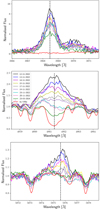 |
Fig. 9 Line evolution of the Ca II H line and H ε (top), the H β line (middle), and the He I D3 line (bottom) during the large flare. The observation times for all spectra are given in the middle panel. For comparison, we include the spectrum with the smallest EW(H α) taken at 23-03-2024 and a spectrum of the inactive K3 giant v UMa for each shown line. |
4.5.2 Timing behaviour during quiescence
To study the time evolution of the stellar activity, we calculated the EW of the H α line, of other chromospheric indicator lines, and a photospheric line for comparison and plotted these in Fig. 10 for both observing seasons. After about the eighth spectrum the influence of the large flare on the shown EWs of the chromospheric lines ceases and a sinusoidal pattern starts to dominate the EWs timing behaviour. All chromospheric lines show a qualitatively consistent behaviour. In the second observing season the pattern in principal resumes but with larger deviations due to flaring activity and also exhibiting some amplitude changes (for example around JD=2460315 and 2460380 d).
If we assume that the pattern is caused by a stable plage region rotating with the star, changes in EW amplitude may occur when the area of the plage region is growing or decaying or when the intensity changes in the emitting area. A sine fit of the EW(H α) values is established for both seasons independently (and excluding the first 12 potentially flare affected spectra), which leads to a slightly higher amplitude in the second season and periods of 21.2 and 21.3 days, respectively. Comparing the sine fits of EW(H α) to the sine fits of RV, we note a slight phase shift between the two, being present for the whole first season and less pronounced in the second season. Since we attribute the RV shifts to the orbital period of the two stars (cf. Sect. 4.2), this suggests synchronous rotation, with the plage region not directly facing the other star. Additionally, we show a comparison between the TESS light curves obtained in sectors 71 and 72 indicating that the star becomes brighter when there is less H α emission, suggesting the presence of a dark spot beneath the chromospherically bright plage. This is further bolstered by the periodic variation in Teff, which are synchronous to the H α variations (and therefore also slightly shifted with respect to RV).
Interestingly, the photospheric reference line at 6439.05 Å shows a slight trend to lower EWs with a Pearson’s correlation coefficient of r = −0.73 and p = 1.0 × 10⁻⁵. Günther et al. (2024) found indications of a period of at least four years duration in the ASAS-SN data they used but cautioned that this may be not true periodic but rather a stochastic episode. Since the large flare occurred at about the maximum brightness of the star not only of the short 21 day period but also of this longer period, our trend would be in agreement with the expected decay of stellar brightness for the next two years, which in turn may be caused by an activity cycle.
4.5.3 Periodic changes in line shape
To further investigate the periodic behaviour of the EWs, we studied the line shapes of various spectral lines during the course of the best covered period between JD=2459930.6 and 2459951.6 days, and additionally at the end of the second observing season from JD =2460371.6 and 2460392.6 days, where the EW(H α) is decreasing from one maximum to the next. We corrected the spectra for the mean RV=16.81 km s−1 of the system and plot the resulting spectra in Figs. A.1 and A.2. Since most clearly H α, but also Ca II K and the IRT lines show some deformations we attribute to the photospheric contribution to the line, we subtracted a PHOENIX model spectrum (since we lack a better template spectrum). We show this purely chromospheric emission also corrected for the individual (photospheric) RV shift of the spectra in Figs. 11 and 12; for comparison we also plot the photospheric Ca I line located at 6439.28 Å. The line demonstrates the deficits of the PHOENIX model but also shows that the model is sufficiently accurate for our purposes, given the much higher amplitudes in the chromospheric lines. The Ca II IRT lines are present as weak absorption lines with emission cores (cf., Figs. A.1 and A.2), with the middle line exhibiting the deepest photospheric absorption component and the bluest line the weakest. Since we want to concentrate here on the chromospheric emission we present in Figs. 11 and 12 the bluest Ca II IRT line. The two figures show that the Na I D lines exhibit a complex behaviour with both an emission and absorption component, and it is not totally clear, whether this is an artefact of the model substraction since it shows similar a structure as the photospheric line albeit with higher amplitude. However, the Na I D lines are known to exhibit complicated line profiles, which may not be fully accounted for by the PHOENIX model. We therefore only state that there is chromospheric line emission in these lines. For the first observing season, H α, Ca II K and less clearly the IRT line show blueshifted emission between phase ∼ 0.2 and ∼ 0.5, which can be best seen in the emergence of a blue peak in Ca II K and in the shift of the steep flank of H α. The emission emerges with the highest blue shift and moves gradually to smaller values, which we interpret as a feature rotating with the star and identify with a plage region located over the large spot. Furthermore, the Ca II K line and even more the H α line are broadened extending the expected rotation profile. For a giant we would not expect pressure broadening in the chromosphere, so this may either indicate turbulent material or part of the emitting material being located above the stellar surface. Since for H α additional emission persists also for the spectrum at about phase = 0.65 (lime green spectrum), while in the Ca II K line the additional emission has vanished for this spectrum, we favour the latter scenario, with H α emission extending to larger heights than for the Ca II K line.
At the end of the second observing season the situation has slightly changed for the chromospheric lines as can be seen in Fig. 12. Although the chromospheric emission is reduced for all lines in the second observing season, the shape of the emission lines has stayed more or less the same. Again for the Ca II K line and the H α line a blue emission component emerges at several phases but for a shorter time than in the first season for Ca II K (from phase 0.3 to 0.5), while for the H α line the additional emission still starts at phase ∼ 0.2 but with less additional emission than in the first observing season. Moreover, the shift to redder wavelengths is not as clearly seen as for the first observing season.
Interestingly, for the spectra at phases ∼ 0.6 and 0.7, an additional emission bump emerges on the red flank of the line with a projected velocity of 20 km s−1 tentatively interpreted as an additional plage region seen at the red shifted edge of the star. In the following spectrum at phase ∼ 0.85, instead a broad absorption feature occurs in the very red wing at around 6566 Å indicating infalling cool material.
To allow for an even more detailed comparison between the two observing seasons for phase ∼ 0.0 and 0.5, we show the spectra with the highest red and blue shift, respectively, of the H α line again in Fig. 13. While a decay in amplitude to the second observing season is seen, also the red wing for the blue shifted spectra is less pronounced in the second observing run (as seen from a comparison of the black to the blue spectrum), while it is more pronounced for the red shifted spectra (red and orange spectrum).
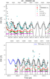 |
Fig. 10 Time evolution of the EW of various lines as designated in the legend of the upper panel. Top: first observing season. Bottom: second observing season. We note, that the EW(Ca IRT) and the EW(Ca I) of the photospheric reference line have been scaled for better display by a factor of 2.5 each. Overplotted are as black solid line the sine fits to the EW(H α) values of the respective season, as dashed black line the sine fit to the RV values of the respective season, and in blue the TESS lightcurves of sector 71 and 72, which have been scaled by a factor of 0.007 and shifted for convenience. We also note that the TESS lightcurve has its maximum count rate for the smallest H α emission (and that therefore the flare displayed here in the TESS lightcurve is ’inverted’). |
4.5.4 The He I IRT and Paschen lines
The CARMENES observations cover also the infrared part of the spectrum, which contains additional chromospheric lines, out of which we show the He I IRT in Fig. 14 and the Pa β line in Fig. 15 with a PHOENIX photospheric spectrum for comparison. While the photospheric model does not predict any absorption or emission at the position of the He I IRT, the Pa β line is predicted as moderate absorption line. Both spectral regions show reasonably good agreement between model and observed spectrum for the photospheric lines; for the chromospheric lines we note deviations, nevertheless.
For the He I IRT the situation is hampered by strong telluric and airglow lines, but there is a blueshifted broad emission component and a similar broad redshifted absorption component present reminiscent of an inverse P Cygni profile. We therefore attempt to fit these broad components with Gaussians. Because of the presence of the telluric lines, the unknown agreement between photospheric observed and model lines for individual lines, and the width of the two Gaussians we can provide only rough estimates as illustrated by the two shown models in Fig. 14 and provide the fit parameters of these two models in Table 6. Despite the model limitations we can state that the involved velocities are large. While the peak velocity of the emitting gas is about 50 km s−1, that of the absorbing material is −50 to −90 km s−1 with wings extending to more than 100 km s−1 in both cases.
The presence of He I IRT is suggestive of high pressures and X-ray and ultraviolet radiation as shown for active M dwarf stars, where the He I IRT is usually observed in absorption; only for flares with high enough pressure to cause the Stark effect in the Balmer lines, the He I IRT line is observed in emission (Fuhrmeister et al. 2019, 2020). At the position of the Pa β line we find additional absorption without any obvious shifts or substructure. We also find additional absorption compared to a PHOENIX model at the position of Pa γ.
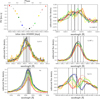 |
Fig. 11 Line shape evolution of various lines as indicated in each panel for the first observing season. For all lines a PHOENIX photospheric model spectrum is subtracted. Top left: RV shift over time of the individual spectra. We show all taken spectra in grey and the colour coding of the spectra shown in the other panels. All other panels: line centre indicated by the vertical dashed broad line, while the narrow dashed vertical lines mark velocities of ±10 km s−1 and ±20 km s−1. |
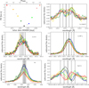 |
Fig. 12 Line shape evolution of various lines as indicated in each panel for the second observing season. For all lines a PHOENIX photospheric model spectrum is subtracted. Top left: RV shift over time of the individual spectra. We show all taken spectra in grey and the colour coding of the spectra shown in the other panels. All other panels: line centre indicated by the vertical dashed broad line, while the narrow dashed vertical lines mark velocities of ± 10 km s−1 and ± 20 km s−1. |
4.5.5 Additional flaring activity
In Fig. 10, several deviations from the periodic behaviour can be noted. We regard the excursions seen there to EW(Ca K)<−-5.0 Å as real and representing higher activity states, which can be explained by flaring. Since we have only coarse time sampling of about one day and longer, it is hard to identify such smaller flares since there is no decay curve observed. Especially for the Ca II K line, which shows more variability than any of the other measured chromospheric indicator lines, other types of variability like short-lived additional plage cannot be ruled out. Nevertheless, we note that the largest deviations from the expected periodic variation occur around activity level maxima as can easily be noted in Fig. 10. Inspection of these spectra reveals an enhanced blue shifted peak for almost all of them, which is expected for this phase, demonstrating that the large spot is facing the observer at these times and is responsible for the additional flux.
In EW(H α) in the first observing season only one possible flare can be noted at JD=2459912 days, which occurs quite shortly after the large flare and does not show a pronounced reaction in EW(Ca K). In the second season a lot more deviations from a purely sinusoidal curve are seen, again with the largest deviations occurring at about the maximum of the periodic activity levels. Here, we also see clear variations in the Ca II IRT line and H β. The behaviour for these H α transients at JD=2460337-2460340 days (three spectra affected) and JD=2460364 days deviates from the Ca II K line, since the EW enhancements are caused mainly by broadening of the H α line, which can be seen in Fig. 16.
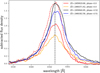 |
Fig. 13 Long time line evolution of H α. We compare here the two spectra with the highest red and blue shift respectively from Figs. 11 and 12. The black and blue lines denote the spectra of phase 0.5 from the first and second season, respectively. The red and orange lines denote the spectra of phase 0. for the first and second season, respectively. Each spectrum has a PHOENIX photospheric model subtracted. We show additionally the red spectrum scaled to match the black spectrum as red dashed line. The dashed vertical black line marks line centre. |
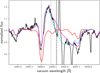 |
Fig. 14 Spectral region around the He I IRT lines. Shown are the CARMENES spectrum (black) and a PHOENIX purely photospheric comparison spectrum (red). We additionally show two possible models with a Gaussian shaped emission and absorption added to the PHOENIX spectrum (cyan and magenta). The vertical dashed lines mark the position of a Si I line at 10830.057 Å, and the three components of the He I IRT. The narrow emission line is an OH airglow line, while the three narrow absorption lines are telluric lines. |
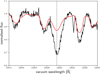 |
Fig. 15 Spectral region around the Pa β line. Shown are the CARMENES spectrum (black) and a PHOENIX purely photospheric comparison spectrum (red). The vertical dashed line marks the position of Pa β. Further absorption lines are a Ti i line at 12814.99 Å, a Ca i line at 12819.55 Å and another Ti i line at 12825.18 Å. |
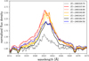 |
Fig. 16 H α line shape for smaller flares in the second observing season. Shown are a spectrum of low activity level (grey), a spectrum of high activity level from the periodic behaviour (black) and the flare spectra from JD=2460337-2460342 days in red, salmon, orange, and yellow (with the first three spectra showing clearly enhanced EW(H α)), and the flare spectrum taken at JD=2460364 days (blue). For the sequence an enhancement and decay of the far blue wing can be noticed. |
5 Discussion
5.1 Superflares
Superflares are typically referred to as flares with energy releases much higher than 1032 erg and some authors choose a threshold above 1033 erg (Notsu et al. 2019). For main sequence stars such enormous energy releases are quite rare (Schmitt et al. 2021), yet for giant stars and in particular RS CVn systems substantially larger energy releases have been reported. For example, Tsuboi et al. (2016) report MAXI X-ray observations of flares on RS CVn systems with some flares reaching (X-ray) energy releases in excess of 1038 erg, and Sasaki et al. (2021) report MAXI detections of 11 flares (in 8 years) on the RS CVn system GT Mus with energy releases again in the range 1038 erg. Karmakar et al. (2023) present detailed Swift observation of a large flare on the RS CVn system SZ Psc with an energy release of about 2 × 1038 erg. With an energy release of more than 1039 erg, the flare event on HD 251108 appears to have even a larger Xray energy release than these previously reported flares on RS CVn systems. The new TESS observations presented and analyzed here show that energy releases on that order do not appear unusual for HD 251108 and, in particular, they may occur even at optical wavelengths.
5.2 Explanations for the periodic RV variations: Spot, binarity, or pulsations
Periodic variations in RV can be caused by stellar spots, binarity, or oscillations. The high amplitude K ∼ 9 km s−1 RV variations with a period of about 21 days described in Sect. 4.2 are hard to explain with oscillations. However, in RV curves of giants oscillations have mimicked planets (Hatzes et al. 2018, e. g.), which potentially arise from non-radial oscillations (Spaeth et al. 2024). These oscillations typically have periods of hundreds of days and only amplitudes of several 100 m s−1 and not about 10 km s−1. Another type of pulsations in giants are p-mode oscillations, but these have typically much shorter periods from hours up to a few days depending on stellar masses, radii, and effective temperatures. Also again, the amplitude of our RV changes is much too high, as p-mode oscillations have typical amplitudes of 10-20 m s−1 (Hatzes & Zechmeister 2008).
The spot and the binary scenario are harder to discern. While the very sinusoidal curve and the high amplitude favour binarity, the change in amplitude and eccentricity from one season to the other favour a star spot. Also the coincidence with the period in photometric magnitude and EW of the chromospheric lines favours the spot scenario. In this scenario, the RV curve variations can be caused by spots rotating with the star and leading to deformations in the line profile; this is a well known effect from RV planet searches, since spots are also able to mimic the imprint of a planet (Queloz et al. 2001; Bonfils et al. 2007; Delgado Mena et al. 2018, 2023). Nevertheless, the expected RV amplitude in RV would be much smaller. While we estimated a compatible RV amplitude of about 10 km s−1 following Aigrain et al. (2012) for spot induced variations, their equation is only valid for point like spots and therefore not applicable here. A more realistic description can be gained with the program nightfall4 (Wichmann 2011). Larger spots give lower amplitude but also more sinusoidal RV variations leading to about 1.5 km s−1 semi-amplitude for an equatorial spot with a filling factor of 0.5. This leads us to a combined scenario of a spot and a low-mass (M dwarf) binary. The system needs to be in synchronous rotation with the spot migrating and evolving during time. As can be seen in Fig. 5, the spot is shifted in phase by 0.5 from the first to the second season. Moreover, in the first season the spot seems to consists only of one component, while in the second season there seems to be a more complicated spot pattern, but still dominated by a very large spot.
This scenario of a synchronously rotating binary system with the giant hosting a large spot would explain the following: (i) The large RV amplitude is induced by the combination of a binary (dominating) and a spot. (ii) The amplitude and shape changes in the RV curve are caused by spot evolution and migration. The observed semi-amplitude of about 1.5 km s−1 of the spot induced residuals is in agreement with the semi-amplitude estimated by our simulations with nightfall. (iii) The phase shift between the period of the EW of the chromospheric lines and the RV curve is about the same in both seasons. Therefore, this cannot be caused by plage residing over the spot, but should be caused by an interaction between the two stars. (iv) The asymmetric profile of the photospheric lines in the CARMENES spectrum is indicative of a phase shifted spot, since the spectrum was taken at low relative RV and any line contribution of the binary object would be expected at line centre. Also the TIGRE averaged line profiles as seen in Fig. 2 support this.
It remains as an intriguing question, why the system is in bound rotation, since typical synchronously rotating systems have periods of lower ten days. For these tight systems the gravitational interaction is much larger and leads to the synchronous rotation.
5.3 Evolutionary stage of HD 251108
Since several contradicting indications of the age of HD 251108 occurred during our analysis, we want to discuss here the evolutionary state of the star. The star shows indications of being a red giant clump star, an RS CVn system, or a young star.
First, the Gaia DR3 catalogue (Gaia Collaboration 2023) lists a Teff = 5099 K and log g = 2.67, where the log g would indicate a red giant clump star. However, we derive from our spectra a variable Teff and log g, but log g>3.0 for all TIGRE spectra and the CARMENES spectrum, which would point to a subgiant. An alternative fit of comparable quality to the CARMENES spectrum would nevertheless also allow for lower values of Teff and lower log g, thereby pointing to a giant (see Sect. 4.1.1). The same is true for the spectral synthesis with MOOG of the averaged TIGRE spectrum. Also, we can estimate the radius: if we interpret the period of our RV curve as rotation period (synchronous rotation) and use our measured v sini values we derive a radius of about 7 R⊙, which is in agreement with estimates by Günther et al. (2024) using magnitude, distance, and temperature. Moreover, using the stellar parameter from the spectral synthesis and the Gaia distance we derive a slightly higher radius of 10 R⊙. Both values are too high for the star being a subgiant (or a young star) with about solar mass.
Regarding the Li line, among giant stars, high activity variability (often correlated to RV) is typically found for lithium rich and lithium enhanced stars (Rolo et al. 2024). While HD 251108 shows correlation between chromospheric line indices and RV, its lithium enhancement stays elusive with A(Li) = 1.26 dex. The presence of Li lines would also fit naturally into the young star scenario, but an obvious Li line is also often observed in RS CVn stars (Pallavicini et al. 1992). Thus, this prevents us from drawing any definitive conclusions.
Also the activity status of HD 251108 may hint at its evolutionary stage. The high activity level and long flaring duration is mostly compatible with those of (long period) RS CVn systems, which are known to show flares lasting longer than one day (Karmakar et al. 2023). Being an RS CVn system would make a subgiant status more probable. Nevertheless, red giant clump stars are capable of producing flares lasting several days as well (Ayres et al. 2001). The persistent and strong emission in H α is uncommon for both active red clump giant stars and (to a lesser degree) for RS CVn systems containing a subgiant (Özdarcan 2021). Persistent H α emission has been reported for one red clump star, which has probably undergone its He flash only very recently and has A(Li) = 3.85 dex (Singh et al. 2024). On the other hand such persistently strong H α emission is most common among young stars in their classical TTauri phase.
Furthermore, for the He I IRT lines we are aware only of detection in absorption for (red clump) giant stars (Sneden et al. 2022), which implies much lower levels of chromospheric activity in these stars. Also for RS CVn stars Zirin (1982) reports He I IRT to be in strong absorption - except for one star, which showed it in emission. On the other hand, the line profile of the He I IRT line is reminiscent of some of the line profiles shown in a study of accretion in young stars by Fischer et al. (2008). Nevertheless, for a young star with He I IRT in emission, one would expect an accretion disk, which would be notable as infrared excess, which is not seen for HD 251108 in Fig. 17 in the spectral energy distribution from archival data. Also, a young star should be much fainter at the distance measured by Gaia.
We therefore conclude in concordance with Günther et al. (2024) that most evidence points to HD 251108 being a red clump giant star, which is much more active than other observed stars in this regime. However, the causes of these extraordinarily high activity levels in HD 251108 currently remain unknown.
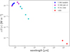 |
Fig. 17 Spectral energy distribution of HD 251108 from ViZier catalogues (Ofek & Frail 2011; Cutri et al. 2012; Bourgés et al. 2014; Gordon et al. 2021; Gaia Collaboration 2022)5 with the two measurements in the radio from catalogues J/ApJS/255/30 and J/ApJ/737/45. |
6 Conclusions
After the occurrence of an X-ray transient on the giant star HD 251108, the TIGRE telescope started spectroscopic monitoring of the star for two observational seasons and collected 149 (82 and 67, respectively) spectra. With this dataset we determined Teff, log g, and v sin i of HD 251108. We found periodic variations in Teff with the same period as our RV and EW measurements. Despite the coincidence in periods of different activity indicators, the amplitude of the RV signal is so large that it has to be caused partly by a binary companion. The secondary component cannot be identified in the photospheric lines; yet this is also not expected, since the binary mass function suggests a mid-M dwarf as the companion. Moreover, the star seems to be in synchronous rotation, since the sinusoidal variations of the EWs of chromospheric lines are indicative of a large plage region rotating with the star and exhibit the same period as the RV variations. Günther et al. (2024) inferred a large spot-filling factor of 0.6, of which changes may cause the changes reported here in terms of the amplitude and shape of the RV curve from one season to the other. We also note that based on the EW behaviour, the spot configuration in the first season directly after the giant flare was much more stable than in the second observing season, where more and more severe EW deviations from the periodic behaviour are observed. Also, we found an additional blue-shifted flux component being present at certain rotation phases in at least the H α and Ca II K line, which may be a direct imprint of a large plage region rotating with the star, which seems to be located above the dark photospheric spot. The high activity level of the star even during quiescence is also underlined by the observation of He I IRT blueshifted emission and redshifted absorption. In addition, the Paschen lines exhibit additional absorption, as compared to a PHOENIX photospheric model.
During the giant flare, we observed an enhancement of several chromospheric lines, namely: the Balmer, Ca II, Na I, and He I lines, but with no emission from the Fe I or Ti I lines that have been observed in K and M dwarf flares (Paulson et al. 2006; Lalitha et al. 2013; Fuhrmeister et al. 2008). The H α line shows the slowest decay of these lines, which is also in contrast to many K and M dwarf flares, where Ca II H&K are often observed to decay at the slowest pace (followed by H α, see e.g. Fig. 9 in Kowalski (2024) and references therein).
Finally, we found contradictions regarding the evolutionary status of the star. While the Gaia distance and its observed brightness clearly point to an evolved star in the red giant clump of the Hertzsprung-Russell-diagram, the observed He I IRT emission (to our knowledge) has not been found in such stars before, yet is a common feature of accreting young stars. This makes HD 251108 an interesting object for a high-resolution monitoring campaign, but also for observations at other wavelength ranges. For example, studies in the infrared, where the presence of a weak accretion disk could be established, would be useful in future investigations.
Data availability
Table A.1 is only available in electronic form at the CDS via anonymous ftp to cdsarc.cds.unistra.fr (130.79.128.5) or via https://cdsarc.cds.unistra.fr/viz-bin/cat/J/A+A/697/A201.
Acknowledgements
The authors acknowledge funding through Deutsche Forschungsgemeinschaft DFG program IDs EI 409/20-1 and SCHN 1382/4-1 in the framework of the YTTHACA project (Young stars at Tübingen, Tautenburg, Hamburg & ESO - A Coordinated Analysis). E.D.M. acknowledges support by the Spanish MICIU/AEI/10.13039/501100011033 and the Ramón y Cajal fellowship RyC2022-035854-I. This research made use of PyAstronomy (Czesla et al. 2019). We thank R. Wichmann for help with nightfall. This research has made use of the VizieR catalogue access tool, CDS, Strasbourg, France (Ochsenbein 1996). The original description of the VizieR service was published in Ochsenbein et al. (2000).
Appendix A Chromospheric line shifts
Here, we show the original chromospheric lines without a photospheric correction and the radial velocity shift only corrected for the systems shift in Figs A.1 and A. 2 for both observing seasons, respectively, as opposed to the spectra corrected with a PHOENIX photospheric spectrum in Figs 11 and 12. We would therefore expect to see shifting lines during the course of the radial velocity period - which is clearly seen for the photospheric reference line. The lower line fluxes for high radial velocity values can also be seen here, although the line centre looks double peaked for the H α and Ca II K line.
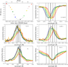 |
Fig. A.1 Line shape evolution of various lines as indicated in each panel for the first observing season. Top left: RV shift over time of the individual spectra. We show all taken spectra in grey and the colour coding of the spectra shown in the other panels. All other panels: Line centre marked with the vertical dashed broad line, while the narrow dashed vertical lines mark velocities of ± 10 km s−1 and ± 20 km s−1. |
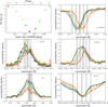 |
Fig. A.2 Line shape evolution of various lines as indicated in each panel for the second observing season. Top left: RV shift over time of the individual spectra. We show all taken spectra in grey and the colour coding of the spectra shown in the other panels. All other panels: Line centre marked with the vertical dashed broad line, while the narrow dashed vertical lines mark velocities of ± 10 km s−1 and ± 20 km s−1. |
References
- Adibekyan, V. Z., Benamati, L., Santos, N. C., et al. 2015, MNRAS, 450, 1900 [Google Scholar]
- Aigrain, S., Pont, F., & Zucker, S. 2012, MNRAS, 419, 3147 [NASA ADS] [CrossRef] [Google Scholar]
- Ayres, T. R., Osten, R. A., & Brown, A. 2001, ApJ, 562, L83 [Google Scholar]
- Bailer-Jones, C. A. L., Rybizki, J., Fouesneau, M., Demleitner, M., & Andrae, R. 2021, AJ, 161, 147 [Google Scholar]
- Baliunas, S. L., Donahue, R. A., Soon, W. H., et al. 1995, ApJ, 438, 269 [Google Scholar]
- Barnes, S. A. 2007, ApJ, 669, 1167 [Google Scholar]
- Bonfils, X., Mayor, M., Delfosse, X., et al. 2007, A&A, 474, 293 [NASA ADS] [CrossRef] [EDP Sciences] [Google Scholar]
- Bourgés, L., Lafrasse, S., Mella, G., et al. 2014, in Astronomical Data Analysis Software and Systems XXIII, eds. N. Manset, & P. Forshay, ASPC, 485, 223 [Google Scholar]
- Caballero, J. A., Guàrdia, J., López del Fresno, M., et al. 2016, Proc. SPIE, 9910, 99100E [Google Scholar]
- Cao, D., Gu, S., Ge, J., et al. 2019, MNRAS, 482, 988 [NASA ADS] [CrossRef] [Google Scholar]
- Cutri, R. M., Wright, E. L., Conrow, T., et al. 2012, Explanatory Supplement to the WISE All-Sky Data Release Products, Explanatory Supplement to the WISE All-Sky Data Release Products [Google Scholar]
- Czesla, S., Schröter, S., Schneider, C. P., et al. 2019, PyA: Python astronomy-related packages, Astrophysics Source Code Library [record ascl:1906.010] [Google Scholar]
- Delgado Mena, E., Lovis, C., Santos, N. C., et al. 2018, A&A, 619, A2 [NASA ADS] [CrossRef] [EDP Sciences] [Google Scholar]
- Delgado Mena, E., Gomes da Silva, J., Faria, J. P., et al. 2023, A&A, 679, A94 [NASA ADS] [CrossRef] [EDP Sciences] [Google Scholar]
- Emslie, A. G., Dennis, B. R., Shih, A. Y., et al. 2012, ApJ, 759, 71 [Google Scholar]
- Ferraz-Mello, S. 1981, AJ, 86, 619 [NASA ADS] [CrossRef] [Google Scholar]
- Fischer, W., Kwan, J., Edwards, S., & Hillenbrand, L. 2008, ApJ, 687, 1117 [Google Scholar]
- Fuhrmeister, B., Liefke, C., Schmitt, J. H. M. M., & Reiners, A. 2008, A&A, 487, 293 [NASA ADS] [CrossRef] [EDP Sciences] [Google Scholar]
- Fuhrmeister, B., Czesla, S., Hildebrandt, L., et al. 2019, A&A, 632, A24 [NASA ADS] [CrossRef] [EDP Sciences] [Google Scholar]
- Fuhrmeister, B., Czesla, S., Hildebrandt, L., et al. 2020, A&A, 640, A52 [NASA ADS] [CrossRef] [EDP Sciences] [Google Scholar]
- Gaia Collaboration. 2022, VizieR On-line Data Catalog: I/360 [Google Scholar]
- Gaia Collaboration (Vallenari, A., et al.). 2023, A&A, 674, A1 [NASA ADS] [CrossRef] [EDP Sciences] [Google Scholar]
- Gondoin, P. 2007, A&A, 464, 1101 [NASA ADS] [CrossRef] [EDP Sciences] [Google Scholar]
- Gondoin, P., Erd, C., & Lumb, D. 2002, A&A, 383, 919 [NASA ADS] [CrossRef] [EDP Sciences] [Google Scholar]
- González-Pérez, J. N., Mittag, M., Schmitt, J. H. M. M., et al. 2022, Front. Astron. Space Sci., 9, 912546 [Google Scholar]
- Gordon, Y. A., Boyce, M. M., O’Dea, C. P., et al. 2021, ApJS, 255, 30 [NASA ADS] [CrossRef] [Google Scholar]
- Günther, H. M., Pasham, D., Binks, A., et al. 2024, ApJ, 977, 6 [Google Scholar]
- Hatzes, A. P., & Zechmeister, M. 2008, JPhCS, 118, 012016 [Google Scholar]
- Hatzes, A. P., Endl, M., Cochran, W. D., et al. 2018, AJ, 155, 120 [NASA ADS] [CrossRef] [Google Scholar]
- Hauschildt, P. H., Allard, F., & Baron, E. 1999, ApJ, 512, 377 [Google Scholar]
- Hawkins, K., Leistedt, B., Bovy, J., & Hogg, D. W. 2017, MNRAS, 471, 722 [Google Scholar]
- Hekker, S., & Meléndez, J. 2007, A&A, 475, 1003 [NASA ADS] [CrossRef] [EDP Sciences] [Google Scholar]
- Hempelmann, A., Mittag, M., Gonzalez-Perez, J. N., et al. 2016, A&A, 586, A14 [NASA ADS] [CrossRef] [EDP Sciences] [Google Scholar]
- Huensch, M., Schmitt, J. H. M. M., Schroeder, K. P., & Reimers, D. 1996, A&A, 310, 801 [NASA ADS] [Google Scholar]
- Husser, T.-O., Wende-von Berg, S., Dreizler, S., et al. 2013, A&A, 553, A6 [NASA ADS] [CrossRef] [EDP Sciences] [Google Scholar]
- Karmakar, S., Naik, S., Pandey, J. C., & Savanov, I. S. 2023, MNRAS, 518, 900 [Google Scholar]
- Kowalski, A. F. 2024, Liv. Rev. Sol. Phys., 21, 1 [Google Scholar]
- Kumar, Y. B., Reddy, B. E., Campbell, S. W., et al. 2020, Nat. Astron., 4, 1059 [Google Scholar]
- Lalitha, S., Fuhrmeister, B., Wolter, U., et al. 2013, A&A, 560, A69 [NASA ADS] [CrossRef] [EDP Sciences] [Google Scholar]
- Lind, K., Asplund, M., & Barklem, P. S. 2009, A&A, 503, 541 [NASA ADS] [CrossRef] [EDP Sciences] [Google Scholar]
- Ling, Z. X., Liu, Y., Zhang, C., et al. 2022, ATel, 15748, 1 [Google Scholar]
- Mittag, M., Hempelmann, A., González-Pérez, J. N., & Schmitt, J. H. M. M. 2010, Adv. Astron., 2010, 101502 [Google Scholar]
- Mittag, M., Schröder, K. P., Hempelmann, A., González-Pérez, J. N., & Schmitt, J. H. M. M. 2016, A&A, 591, A89 [NASA ADS] [CrossRef] [EDP Sciences] [Google Scholar]
- Mittag, M., Hempelmann, A., Fuhrmeister, B., Czesla, S., & Schmitt, J. H. M. M. 2018, AN, 339, 53 [Google Scholar]
- Notsu, Y., Maehara, H., Honda, S., et al. 2019, ApJ, 876, 58 [Google Scholar]
- Ochsenbein, F. 1996, The VizieR database of astronomical catalogues [Google Scholar]
- Ochsenbein, F., Bauer, P., & Marcout, J. 2000, A&AS, 143, 23 [NASA ADS] [CrossRef] [EDP Sciences] [Google Scholar]
- Ofek, E. O., & Frail, D. A. 2011, ApJ, 737, 45 [NASA ADS] [CrossRef] [Google Scholar]
- Oláh, K., Seli, B., Kővári, Z., Kriskovics, L., & Vida, K. 2022, A&A, 668, A101 [NASA ADS] [CrossRef] [EDP Sciences] [Google Scholar]
- Özdarcan, O. 2021, PASA, 38, e027 [Google Scholar]
- Paegert, M., Stassun, K. G., Collins, K. A., et al. 2022, VizieR On-line Data Catalog: TESS Input Catalog version 8.2 IV/39 [Google Scholar]
- Pallavicini, R., Randich, S., & Giampapa, M. S. 1992, A&A, 253, 185 [NASA ADS] [Google Scholar]
- Pasham, D., Hamaguchi, K., Miller, J. M., et al. 2022, ATel, 15755, 1 [Google Scholar]
- Paulson, D. B., Allred, J. C., Anderson, R. B., et al. 2006, PASP, 118, 227 [Google Scholar]
- Queloz, D., Henry, G. W., Sivan, J. P., et al. 2001, A&A, 379, 279 [NASA ADS] [CrossRef] [EDP Sciences] [Google Scholar]
- Quirrenbach, A., CARMENES Consortium, Amado, P. J., et al. 2020, SPIE, 11447, 114473C [Google Scholar]
- Ricker, G. R., Winn, J. N., Vanderspek, R., et al. 2015, JATIS, 1, 014003 [Google Scholar]
- Rolo, I., Delgado Mena, E., Tsantaki, M., & Gomes da Silva, J. 2024, A&A, 688, A68 [NASA ADS] [CrossRef] [EDP Sciences] [Google Scholar]
- Sasaki, R., Tsuboi, Y., Iwakiri, W., et al. 2021, ApJ, 910, 25 [NASA ADS] [CrossRef] [Google Scholar]
- Schmitt, J. H. M. M., Ioannidis, P., Robrade, J., et al. 2021, A&A, 652, A135 [NASA ADS] [CrossRef] [EDP Sciences] [Google Scholar]
- Schmitt, J. H. M. M., Schröder, K.-P., Rauw, G., et al. 2014, AN, 335, 787 [NASA ADS] [Google Scholar]
- Schröder, K. P., Schmitt, J. H. M. M., Mittag, M., Gómez Trejo, V., & Jack, D. 2018, MNRAS, 480, 2137 [CrossRef] [Google Scholar]
- Singh, R., Mallick, A., Reddy, B. E., Pandey, J. C., & Zhao, G. 2024, ApJ, 971, L3 [Google Scholar]
- Sneden, C., Afşar, M., Bozkurt, Z., et al. 2022, ApJ, 940, 12 [NASA ADS] [CrossRef] [Google Scholar]
- Sneden, C. A. 1973, PhD thesis, University of Texas, Austin, USA [Google Scholar]
- Spaeth, D., Reffert, S., Hunt, E. L., Kaminski, A., & Quirrenbach, A. 2024, A&A, 689, A91 [NASA ADS] [CrossRef] [EDP Sciences] [Google Scholar]
- Tsantaki, M., Andreasen, D., & Teixeira, G. 2023a, FASMA: Stellar spectral analysis package, Astrophysics Source Code Library [record ascl:2311.014] [Google Scholar]
- Tsantaki, M., Delgado-Mena, E., Bossini, D., et al. 2023b, A&A, 674, A157 [NASA ADS] [CrossRef] [EDP Sciences] [Google Scholar]
- Tsuboi, Y., Yamazaki, K., Sugawara, Y., et al. 2016, PASJ, 68, 90 [NASA ADS] [CrossRef] [Google Scholar]
- Wichmann, R. 2011, Nightfall: Animated Views of Eclipsing Binary Stars, Astrophysics Source Code Library [record ascl:1106.016] [Google Scholar]
- Xing, L. F., & Xing, Q. F. 2012, A&A, 537, A91 [NASA ADS] [CrossRef] [EDP Sciences] [Google Scholar]
- Zechmeister, M., & Kürster, M. 2009, A&A, 496, 577 [CrossRef] [EDP Sciences] [Google Scholar]
- Zechmeister, M., Anglada-Escudé, G., & Reiners, A. 2014, A&A, 561, A59 [NASA ADS] [CrossRef] [EDP Sciences] [Google Scholar]
- Zirin, H. 1982, ApJ, 260, 655 [NASA ADS] [CrossRef] [Google Scholar]
Accessible through: https://vizier.cds.unistra.fr/
All Tables
All Figures
|
Fig. 1 Best-fitting stellar parameters versus time. The black dots depict the parameters obtained from the TIGRE spectra and the red diamond the parameters obtained from the CARMENES spectrum. |
| In the text | |
|
Fig. 2 Line profile evolution of an average line profile of nine Fe I lines. The colour scale gives the difference of the normalised flux density to the (also normalised) mean spectrum. The black line marks our RV determination from Sect. 4.2 with its mean shifted to zero RV for display convenience. |
| In the text | |
|
Fig. 3 Top: asymmetry of the photospheric Ca I line at 6440.8 Å. We show the CARMENES spectrum in black. The asymmetry can be noted as weak bump at about 6441.2 Å. For comparison we also show a PHOENIX model spectrum with Teff = 4600 K and log g = 3.5 in red and with Teff = 4400 K and log g = 2.5 in blue. Bottom: zoom on the Ca I line at 6464.36 Å. The asymmetry there is even more severe and suggests that the stellar spectrum should be fitted with a two temperature model. |
| In the text | |
|
Fig. 4 TIGRE RV data: panel a shows the obtained RV values of the individual spectra (black dots) versus time and the red solid line depicts the RV fit. Panel b shows the residuals. Panel c the periodogram of the GLS analysis. Panel d the phased folded RV data, with the data from observing season 2022/2023 shown as black dots and from 2023/2024 as magenta dots, while the red solid line represents the RV fit in phase. |
| In the text | |
|
Fig. 5 RV residuals to sinusoidal fit like in Fig. 4b, but phase-folded. We can notice strong spot migration and evolution from one season to the other. Also, there is more evolution in the second season. |
| In the text | |
|
Fig. 6 Fit of the Li I 6707 Å line using the TIGRE mean spectrum. The lithium abundance is quite robust against changes in log g as can be seen when comparing the value obtained using the spectroscopically determined log g = 2.85 with the one using the trigonometrically determined log g = 2.43. |
| In the text | |
|
Fig. 7 TESS FFI light curve for sector 71 (blue data points) and sector 72 (red data points). |
| In the text | |
|
Fig. 8 Flare light curves of the three flares: original data (blue points), reference data (light curve shifted backwards and forwards by one period; see text for details; green points) together with polynomial fit (solid red line), and net flare light curve (black points). |
| In the text | |
|
Fig. 9 Line evolution of the Ca II H line and H ε (top), the H β line (middle), and the He I D3 line (bottom) during the large flare. The observation times for all spectra are given in the middle panel. For comparison, we include the spectrum with the smallest EW(H α) taken at 23-03-2024 and a spectrum of the inactive K3 giant v UMa for each shown line. |
| In the text | |
|
Fig. 10 Time evolution of the EW of various lines as designated in the legend of the upper panel. Top: first observing season. Bottom: second observing season. We note, that the EW(Ca IRT) and the EW(Ca I) of the photospheric reference line have been scaled for better display by a factor of 2.5 each. Overplotted are as black solid line the sine fits to the EW(H α) values of the respective season, as dashed black line the sine fit to the RV values of the respective season, and in blue the TESS lightcurves of sector 71 and 72, which have been scaled by a factor of 0.007 and shifted for convenience. We also note that the TESS lightcurve has its maximum count rate for the smallest H α emission (and that therefore the flare displayed here in the TESS lightcurve is ’inverted’). |
| In the text | |
|
Fig. 11 Line shape evolution of various lines as indicated in each panel for the first observing season. For all lines a PHOENIX photospheric model spectrum is subtracted. Top left: RV shift over time of the individual spectra. We show all taken spectra in grey and the colour coding of the spectra shown in the other panels. All other panels: line centre indicated by the vertical dashed broad line, while the narrow dashed vertical lines mark velocities of ±10 km s−1 and ±20 km s−1. |
| In the text | |
|
Fig. 12 Line shape evolution of various lines as indicated in each panel for the second observing season. For all lines a PHOENIX photospheric model spectrum is subtracted. Top left: RV shift over time of the individual spectra. We show all taken spectra in grey and the colour coding of the spectra shown in the other panels. All other panels: line centre indicated by the vertical dashed broad line, while the narrow dashed vertical lines mark velocities of ± 10 km s−1 and ± 20 km s−1. |
| In the text | |
|
Fig. 13 Long time line evolution of H α. We compare here the two spectra with the highest red and blue shift respectively from Figs. 11 and 12. The black and blue lines denote the spectra of phase 0.5 from the first and second season, respectively. The red and orange lines denote the spectra of phase 0. for the first and second season, respectively. Each spectrum has a PHOENIX photospheric model subtracted. We show additionally the red spectrum scaled to match the black spectrum as red dashed line. The dashed vertical black line marks line centre. |
| In the text | |
|
Fig. 14 Spectral region around the He I IRT lines. Shown are the CARMENES spectrum (black) and a PHOENIX purely photospheric comparison spectrum (red). We additionally show two possible models with a Gaussian shaped emission and absorption added to the PHOENIX spectrum (cyan and magenta). The vertical dashed lines mark the position of a Si I line at 10830.057 Å, and the three components of the He I IRT. The narrow emission line is an OH airglow line, while the three narrow absorption lines are telluric lines. |
| In the text | |
|
Fig. 15 Spectral region around the Pa β line. Shown are the CARMENES spectrum (black) and a PHOENIX purely photospheric comparison spectrum (red). The vertical dashed line marks the position of Pa β. Further absorption lines are a Ti i line at 12814.99 Å, a Ca i line at 12819.55 Å and another Ti i line at 12825.18 Å. |
| In the text | |
|
Fig. 16 H α line shape for smaller flares in the second observing season. Shown are a spectrum of low activity level (grey), a spectrum of high activity level from the periodic behaviour (black) and the flare spectra from JD=2460337-2460342 days in red, salmon, orange, and yellow (with the first three spectra showing clearly enhanced EW(H α)), and the flare spectrum taken at JD=2460364 days (blue). For the sequence an enhancement and decay of the far blue wing can be noticed. |
| In the text | |
|
Fig. 17 Spectral energy distribution of HD 251108 from ViZier catalogues (Ofek & Frail 2011; Cutri et al. 2012; Bourgés et al. 2014; Gordon et al. 2021; Gaia Collaboration 2022)5 with the two measurements in the radio from catalogues J/ApJS/255/30 and J/ApJ/737/45. |
| In the text | |
|
Fig. A.1 Line shape evolution of various lines as indicated in each panel for the first observing season. Top left: RV shift over time of the individual spectra. We show all taken spectra in grey and the colour coding of the spectra shown in the other panels. All other panels: Line centre marked with the vertical dashed broad line, while the narrow dashed vertical lines mark velocities of ± 10 km s−1 and ± 20 km s−1. |
| In the text | |
|
Fig. A.2 Line shape evolution of various lines as indicated in each panel for the second observing season. Top left: RV shift over time of the individual spectra. We show all taken spectra in grey and the colour coding of the spectra shown in the other panels. All other panels: Line centre marked with the vertical dashed broad line, while the narrow dashed vertical lines mark velocities of ± 10 km s−1 and ± 20 km s−1. |
| In the text | |
Current usage metrics show cumulative count of Article Views (full-text article views including HTML views, PDF and ePub downloads, according to the available data) and Abstracts Views on Vision4Press platform.
Data correspond to usage on the plateform after 2015. The current usage metrics is available 48-96 hours after online publication and is updated daily on week days.
Initial download of the metrics may take a while.