| Issue |
A&A
Volume 689, September 2024
|
|
|---|---|---|
| Article Number | A103 | |
| Number of page(s) | 11 | |
| Section | Stellar structure and evolution | |
| DOI | https://doi.org/10.1051/0004-6361/202348343 | |
| Published online | 13 September 2024 | |
Properties of flare events based on light curves from the TESS survey
II. 20-second cadence
1
College of Physics, Guizhou University, 550025 Guiyang, PR China
2
Department of Physics and Astronomy and SARA, Butler University, Indianapolis, IN 46208, USA
3
Department of Physics & Astronomy, Howard University, Washington, DC 20059, USA
Received:
21
October
2023
Accepted:
10
June
2024
Abstract
Aims. Stellar flares are sudden bursts of energy and are the result of magnetic activity. We used light curves from the TESS 20-second cadence survey from 2020 to 2023 to detect flare events and determine their properties.
Methods. By means of repeated fitting to distinguish stellar background light curves and flare events, we detected 32 978 flare events associated with 5463 flaring stars. Furthermore, we cross-matched our samples with the Gaia and SDSS surveys, obtaining additional stellar parameters that we used to determine the relationships between stellar and flare properties.
Results. We find that the durations of 55% of the studied flares were less than 8 minutes. The flare energies of the TESS 20-second cadence data are typically lower than those obtained from TESS 2-minute cadence data. We identify 28 425 flare events associated with 4784 flaring stars. The relationships between the flare energy and duration for both giant and main sequence stars display a consistent V-shaped distribution, with 1034 erg the midway point. Stars with lower effective temperatures and masses generate more frequent flare events. In summary, it is necessary to detect more flare events with a higher time resolution, and our flare samples with 20-second cadences allowed us to discover additional new properties.
Key words: stars: activity / stars: flare
Corresponding author; This email address is being protected from spambots. You need JavaScript enabled to view it. .
© The Authors 2024
 Open Access article, published by EDP Sciences, under the terms of the Creative Commons Attribution License (https://creativecommons.org/licenses/by/4.0), which permits unrestricted use, distribution, and reproduction in any medium, provided the original work is properly cited.
This article is published in open access under the Subscribe to Open model. This email address is being protected from spambots. You need JavaScript enabled to view it. to support open access publication.
1. Introduction
Stellar flares are sudden bursts of energy and are a result of magnetic activity. A larger number of stellar flares have been detected by analyzing larger datasets from ground and space photometric surveys (Shibayama et al. 2013; Yang et al. 2017; Günther et al. 2020; Jackman et al. 2021). This is important not only for more accurately determining the relationships between the stellar flares and the star’s physical parameters, but also for further developing the stellar dynamo theory associated with such phenomena.
Due to the increase in photometric surveys, astronomers have been actively determining stellar parameters and magnetic activity properties, including starspot and flare parameters (Davenport 2016; Doyle et al. 2019; Günther et al. 2020). Low-mass stars with temperatures of less than 4000 K produce higher flare energies and higher flare rates than hotter stars across stellar ages (Tu et al. 2020; Feinstein et al. 2020; Gao et al. 2022). Quasiperiodic oscillations during the decay time were discovered by Vida et al. (2019) and have been attributed to quasiperiodic motions of the emitting plasma or oscillatory reconnections. From an examination of the distribution on the stellar surface, it has been suggested that flares might be independent of the orbital phase (Doyle et al. 2020; Huang et al. 2020). More, long-duration series of data from photometric surveys are needed to determine the precise relationship between the flare position and the orbital phase. The relationship between stellar and flare parameters, such as the flare amplitude, stellar rotation period, or the Rossby number, has been studied by Howard et al. (2020) and Pietras et al. (2022). The authors confirm that stars with short-period rotators have higher superflare rates and higher flare energies than long-period stars.
While previous research has provided valuable insights into many flare properties, a detailed investigation of flare characteristics, including the substructure of flare events, is still lacking. We can use light curves with a high time resolution, such as the 1-minute cadence data provided by the Kepler mission and the 20-second cadence data released by the Transiting Exoplanet Survey Satellite (TESS) mission, to seek additional information and make more targeted advancements. Stellar flares can last from mere seconds to hours (Moffett 1974; Yang et al. 2023). The energy, amplitude, and duration of flares are influenced by the different time resolutions of the Kepler data (Yang et al. 2018). Light curves with a cadence of about 1 min allow us to better determine and qualify flare shapes and durations compared to higher time resolutions (Lin et al. 2022). Utilizing 13-second cadence light curves from the Next Generation Transit Survey (Wheatley et al. 2018), Jackman et al. (2021) identified associated flare properties, revealing that many short-duration flares go unnoticed in Kepler and TESS cadence surveys. Employing 20-second cadence TESS light curves, Howard & MacGregor (2022) detected 3792 stellar flares from 226 low-mass flare stars. They also identified 49 candidate quasiperiodic pulsations in flare events and confirmed 17 flares exhibiting quasiperiodic pulsations in the rise or decay phase. A 1-second cadence survey of M flare dwarf stars conducted by Aizawa et al. (2022) detected 22 flares with rising times ranging from 5 to 100 seconds. They estimated an occurrence rate of 0.7 flares per day per active star, consistent with other magnetically active M dwarfs. Additionally, Tovar Mendoza et al. (2022) investigated how flares change across observational cadences, ranging from 10 min and 2 min, and including 20-second exposure times.
This current paper marks our second exploration of flare properties using light curves from the TESS mission. In the present study, we delve into the characteristics of flare events with shorter durations, utilizing the 20-second cadence data provided by TESS. Section 2 outlines the TESS data and the targets of our study. The methodology for detecting flare events and calculating the flare energy is detailed in Section 3. A comprehensive statistical analysis of the parameters associated with flaring stars and flare events is presented in Section 4. We conclude with a summary of our findings in Section 5.
2. TESS data
TESS is a space telescope that aims to conduct an all-sky transit survey to discover hundreds of transiting planets smaller than Neptune (Ricker et al. 2015). From July 25, 2018, to July 4, 2020, TESS primarily focused on investigating stars with spectral types from F5 to M5. After this period, the scope of TESS expanded beyond exoplanet searches, incorporating requests to study approximately 10 000 additional objects per cycle through the Guest Investigator program. Starting from July 2020, TESS began observations at a 20-second cadence for certain targets, alongside its original 2-minute cadence photometric monitoring. The extensive 2-minute cadence data have significantly improved our understanding of the general laws of flare events, whereas the 20-second cadence mode allows for the detection of smaller flare occurrences. Our current research initially focused on the 20-second cadence light curves from sectors 27–63, recorded at a 20-second cadence.
3. Flare detection
A flare is characterized as a sudden, significant burst of energy, evident from a noticeable variation in the light curve. This typically includes a rapid rise, averaging around 8.8 minutes, followed by a gradual decay, lasting about 33.7 minutes, as indicated by findings from the Kepler 1-minute cadence survey (Yan et al. 2021). Building on the flare detection methodology outlined in our previous work (Yang et al. 2023; Meng et al. 2023), we have refined our approach of repeated polynomial fitting in order to differentiate between stellar background light curves and flare events more effectively, by eliminating background light from the original data.
Initially, we processed the flux and time data extracted from TESS’s optical light curve files, utilizing the simple aperture photometric flux (PDCSAP flux), which has been corrected by the instrument system for the flux data. The average PDCSAP flux (FPDC) and its normalized value (Fnorm) were calculated as follows:
 (1)
(1)
 (2)
(2)
where Fmax and Fmin represent the maximum and minimum flux values, respectively.
To detect flare events in the normalized light curves, we first estimated the stellar period by fitting the light curve. We then divided the light curve based on this period to improve the background fit, thereby minimizing the impact of the light variation period on flare detection. Each section of the light curve was fitted with a polynomial to derive the best-fit background light curve, characterized by a standard deviation, σ. Through iterative fitting, we could distinguish flare events from stellar light variations more accurately. After subtracting the background light curve, we obtained the detrended light curves. Points exceeding a threshold of three times the standard deviation, 3σ, were flagged as flare candidates. A flare event was confirmed if it comprised at least four consecutive candidate points that matched the profile of a rapid rise followed by a slow decline. The peak of the flare was identified by the maximum luminosity point, with the flare amplitude defined accordingly. The start and end times of the flare event were determined by the timestamps of the first and last points, respectively. A visual inspection was also conducted to validate the findings derived from the automated analysis.
Ultimately, we identified 32 978 flare events across 5463 stars and calculated the bolometric energy of these events (Eflare) using the formula provided by Petrucci et al. (2024, further details regarding the calculation of the bolometric energy from Kepler data are available in Hawley et al. 2014):
 (3)
(3)
where Ebol denotes the bolometric energy of the flares, and ED is the area under the flare light curve, which we call the equivalent duration. LTESS is the quiescent luminosity obtained by considering the TESS CCD response, and c is a correction factor of 0.19 for the TESS CCD response (Howard & MacGregor 2022; Petrucci et al. 2024). The parameters of the flare events are listed in Table A.1 which is presented in Appendix A.
4. Discussion
For the analysis of 32 978 flare events and 5463 stars flares, we cross-referenced the TESS results with catalogs from other surveys, specifically the Sloan Digital Sky Survey (SDSS; Alam et al. 2015) and Gaia (Gaia Collaboration 2023), to acquire supplementary stellar parameters. We also identified 124 eclipsing binary stars, but due to the small sample size, they will not be considered separately in subsequent studies. In this section we discuss the statistical analysis performed on both the stellar and flare characteristics of the subjects studied.
4.1. The distribution of flare durations and peak amplitudes
We performed a statistical analysis of the duration of flare events, as shown in Figure 1. Yang et al. (2023) find that 71% of the flare events they studied based on 2-minute cadence data lasted less than one hour. From our TESS 20-second cadence results, 55% of flare event occurrences were shorter than 8 minutes, indicating a significant detection of short-duration flares that the 2-minute cadence data failed to capture. Several flares exceeded an hour, with the longest reaching 76 minutes. This capability of the TESS 20-second cadence data to uncover numerous short-duration flares gives us a way to investigate smaller flare phenomena. A similar statistical analysis of the amplitude of these flare events shows a distribution that is largely in agreement with findings from the 2-minute cadence sample.
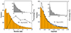 |
Fig. 1. Distributions of flare duration (left) and amplitude (right). The left vertical axes represent the number of flare events, and the right ones represent their corresponding proportions. The orange bars represent the main distribution of the flare duration (or amplitude) based on the TESS 20-second cadence data, while the remaining part of the distribution is shown with the gray bars in the inset. The black dotted line is the distribution of the flare numbers for the TESS 2-minute data (Yang et al. 2023). Due to the inability to search for flare events shorter than 6 minutes in the 2-minute cadence data, the first point’s value in the left panel is zero. |
4.2. Flare energy
Figure 2 shows the energy distributions of flares captured by the TESS 20-second cadence and the TESS 2-minute cadence data (Yang et al. 2023). For clarity, we normalized the flare event peaks across various energy ranges. The right panel of Figure 2 succinctly illustrates the completeness of our current data sample. A comparison between the two panels shows that there is a greater likelihood of detecting lower-energy flares in the TESS 20-second cadence data as compared to the 2-minute cadence data.
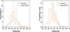 |
Fig. 2. Percentage and normalized count of flare events in different flare energy intervals. Left: proportion of flare events within each energy range. Right: normalized value of the counts of flare events within each energy range shown. The orange lines show the distribution of the flare energy based on the TESS 20-second cadence data, and the dashed gray lines the TESS 2-minute cadence data (Yang et al. 2023). |
4.2.1. Flare energy and stellar parameters
We used the catalog comprising 177 911 stars in the Kepler field provided by Berger et al. (2018) as a reference to determine the evolutionary stage of our sample based on effective temperature and log g. By extracting the Gaia bp_rp color index and the G-band magnitude from Gaia Data Release 3 (Gaia Collaboration 2023), we derived the absolute magnitude using the formula MG = G + 5log(Plx/100) and plot the Hertzsprung−Russell (H−R) diagram in Figure 3. Our results reveal a clustering of stars in the lower-left corner of the main sequence. Following Xing et al. (2024), we classified the stars in this area of the H–R diagram as compact stars (e.g., hot subdwarfs and white dwarfs). Given the rarity of magnetism in these stars, the authenticity of flare events observed and associated with them remains uncertain. Consequently, we omit these from subsequent discussions. We also removed some missing data that cannot be plotted in the H–R diagram. Focusing solely on the remaining sample, comprising 28 425 flare events associated with 4784 flaring stars, we divided it into three categories: main sequence stars, subgiants, and red giants.
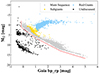 |
Fig. 3. Distribution of the evolution stages of flaring stars. The dashed red line marks the lower edge of the main sequence; the stars below the line are represented by black dots and are not considered in subsequent discussions. Gray, yellow, and blue dots represent main sequence stars, subgiants, and red giants, respectively. |
In Figure 4 we plot the relationship between flare energy and stellar parameters, including stellar mass and effective temperature (Teff). The detection of flares has a selection effect because lower-energy flares can only be seen on fainter stars. The upper panel of Figure 4 shows a positive correlation between the stellar mass and energy, especially for the main sequence stars, which is consistent with previous findings (Lin et al. 2019; Yang et al. 2023). The lower panel illustrates the relationship between stellar temperature and flare energy. For the main sequence stars, there is also a positive correlation between flare energy and temperature, which confirms the conclusion of Yang et al. (2023), that this observed correlation is likely a selection effect: it is what we would expect in a relative-flux-limited survey. Because the numbers of data points for the subgiants and red giants are limited, we do not discuss the relationships between the flare energy as a function of mass or stellar temperatures.
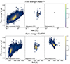 |
Fig. 4. Relationships between the flare energy and the stellar mass (top) and stellar temperature (bottom). We have separated our samples into three evolution stages (main sequence stars, subgiants, and red giants). The n represents the number of points in the panel. |
4.2.2. The relationship between flare energy and its duration
Generally speaking, it is important to explore the correlation between flare energy and flare duration in order to determine the relationships between stellar parameters and solar flares (Tu et al. 2021). The left panel of Figure 5 shows the relationship between flare energy and duration for the entire sample dataset. Both giant and main sequence stars display a consistent V-shaped distribution. The right panel shows a zoomed-in view of the region with durations of less than 10 minutes. Here we observe that, with an energy of 1034 erg as the dividing line, there is a positive correlation trend between the flare energy and duration in both the upper and lower parts (above and below 1034 erg), although the trend above it shows a shorter duration (light yellow part). To determine the reasons for this V-shape appearance, we analyzed the relationship between stellar parameters, flare characteristics, and the flare event duration separately, as shown in Figure 6. Our discussion here focuses on the main sequence stars and giants separately, and there is a substantial decrease in the sample count starting from durations of approximately 4 minutes, with amplitudes ranging from 1 to 10, effective temperatures between 6000 and 8000 K, radii spanning 1–100 R⊙, and masses of 1–3 M⊙.
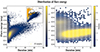 |
Fig. 5. Distribution of flare energies in different duration intervals. Left: relationship between flare energy and duration. The color of the points represents the number density in different regions, with brighter colors indicating a higher number of data points. Note that we use yellow circles to represent the distribution of giants in the small panel, but it does not mean that only giants exist in the positions covered by the yellow circles. Right: details of the flare duration in the 0–10 minute range of the left panel. We have narrowed the scope of the color chart. |
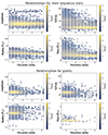 |
Fig. 6. Relationships between flare duration and: flare amplitude, stellar temperature, radius, and mass, respectively. The top four panels show the distribution results for the main sequence stars, while the bottom four panels show the distribution results for giants. The points correspond to the flare events. |
Figure 7 shows the correlation between flare duration and energy for the main sequence star samples of various spectral types. There is a clear correlation between the duration and flare energy for the main sequence stars, especially for the F-, G-, K- and M-type samples. We refrained from depicting the relationships between flare energy and duration for giants because of the scarcity of giants of different spectral types.
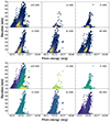 |
Fig. 7. Relationships between flare energy and duration for samples of different spectral types. Upper panel: density of points in different regions (brighter colors indicate a higher number of points). Lower panel: flaring star’s temperature. Note that we have sorted the data by temperature, with points with higher temperatures plotted higher up in the graph. |
Figure 8 illustrates the relationship between flare duration and energy across the three evolutionary stages. A distinct lower edge of the distribution for the main sequence and subgiant stages suggests that as the duration increases, the minimum flare energy gradually rises. The main sequence stars are more inclined to produce small flares with energies of less than 1033 erg. Notably, samples across all three stages are concentrated in regions with short flare durations. The energy released by the flares on stars with higher surface temperatures is generally higher, as clearly demonstrated by the main sequence stars and subgiants in our sample. The detection of flare events hinges on significant photometric light curve variations during the flare phase. Flaring stars with higher temperatures exhibit higher intrinsic luminosities, potentially obscuring weaker flares in the light curve. Consequently, flares detected on stars with higher temperatures tend to release more energy, as seen from the lower limit of the energy range plotted in Figure 7 for samples of different spectral types.
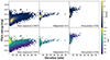 |
Fig. 8. Relationships between flare energy and duration for the different revolution stages: main sequence stars (left), subgiants (middle), and red giants (right). In the top panels, the color scale represents the number density of the data in different locations. The color distributions in different evolution stages are similar, and they are concentrated in regions with short flare durations. In the bottom panels, the color scale represents the stellar temperature of the flaring star. We sorted the data by temperature, with points with higher temperatures higher up in the graph. The n represents the number of flare events; due to some samples missing temperature parameters, the value of n varies. |
In conclusion, we have observed a unique relationship between duration and released energy, T ∝ Eγ, for durations longer than 10 minutes. However, within the 0–10 minute range, a branch emerges, indicating that short-duration flare events can also unleash significant energy.
4.3. Flare frequency distribution
According to previous research (Crosby et al. 1993; Maehara et al. 2015, 2021; Karoff et al. 2016; Tu et al. 2020, 2021), the flare frequency distribution follows a power law, namely dN/dE ∝ E−α. Analysis of solar-type samples from various telescope data reveals α values hovering around 2. In Figure 9 we depict the power-law distribution of the entire sample as well as subsamples categorized by spectral type. The α value for all samples is determined to be 1.52 ± 0.07. Studies by Audard et al. (2000), Lin et al. (2019), and Yang & Liu (2019) delved into power-law analyses for different spectral types. Audard et al. (2000) found α values of 2.28, 1.87, and 1.84 for F-, K-, and M-type stars, respectively, indicating a gradual flattening of the flare frequency distribution with spectral type. Lin et al. (2019) observed a gradual decrease in α until M-type and K-type stars exhibit similar values. Conversely, Yang & Liu (2019) report a decrease followed by an increase in α from F-type to M-type stars, with K-type stars marking the inflection point. Notably, the α value for A-type stars is determined to be 1.17 ± 0.22, which is markedly lower than previous findings. For F- to M-type stars, α values are in the ranges 1.62 ± 0.15, 1.55 ± 0.13, 1.42 ± 0.07, and 1.50 ± 0.05, respectively, exhibiting a decreasing-then-increasing trend with K-type stars as the turning point, consistent with the findings of Yang & Liu (2019).
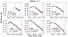 |
Fig. 9. Flare frequency distributions for different spectral types and the whole sample, demonstrating the power-law index. N represents the number of flare events of the sample, and the number of flaring stars is indicated in parentheses. The second blue vertical lines show the true end of the data, but the starting positions of the data (first blue lines) are slightly truncated. The vertical dashed red lines represent the fitting range. The gray lines are all the fitted results of the Markov chain Monte Carlo method, and the solid red line is the final result. |
4.4. Rise and decay times
Flare events are characterized by a swift increase followed by a gradual decrease in stellar luminosity. Using the peak point of the flare event as the demarcation between rise and decay stages, we depict the distribution of rise and decay times in Figure 10, which is similar to the results of Yan et al. (2021). Additionally, we plot the distribution results obtained by Yang et al. (2023) using TESS 2-minute cadence data in insets. Notably, the normal distribution curve of rise times for TESS 20-second data is more complete, suggesting that the 20-second cadence data improved accuracy in determining the flare rise time, especially for the short-duration flares, compared to the 2-minute cadence mode. Consequently, short-cadence data offer more precise details of flare events.
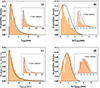 |
Fig. 10. Probability distributions of the rise (top panel) and decay times (bottom panel) based on 20-second data; the insets show the results based on TESS 2-minute data (Yang et al. 2023). The dark lines are their fittings of the bar graph. The left panel uses a decimal scale, and the right panel uses the corresponding log-normal values. |
Building upon the discussion on the relationship between flare duration and energy from Section 4.2.2, we next divided the duration into rise and decay times. Figure 11 reveals no significant correlation between the rise time of flare events and the energy they release. However, a clearer correlation is observed between the energy and decay times, akin to the relationships between energy and duration discussed earlier. Such a correlation is related to a larger proportion of the slow decline phase in the luminosity changes being caused by flare events.
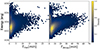 |
Fig. 11. Relationships between energy and the rise (left) and decay times (right). |
4.5. Flare occurrence percentage distribution
We computed the flare occurrence percentage for each flaring star, which is defined as the ratio of the total flaring time (∑tflare) to its corresponding observational time (∑tstar), expressed as a percentage:
 (4)
(4)
These percentages are presented in Figure 12 and consistently align with previous findings by Yang et al. (2023). Furthermore, we investigated the relationship between the flare occurrence percentage, the stellar temperature, and the mass of the flaring star, as illustrated in Figure 13. Notably, stars within the temperature range of approximately 3000–6000 K exhibit higher flare occurrence percentages than hotter stars. Additionally, stars with stellar masses of less than 1.5 M⊙ have a higher flare occurrence percentage, suggesting that stars with lower effective temperatures and masses tend to produce flares more frequently.
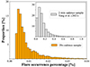 |
Fig. 12. Distribution of the flare occurrence percentage based on the 20-second data. The results based on the TESS 2-minute data are shown in the insets (Yang et al. 2023). The vertical axis shows the ratio of samples in the corresponding bin to the full sample. |
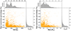 |
Fig. 13. Relationships between the flare occurrence percentage and the stellar temperature (left panel) and the mass (right panel). The orange dots represent our sample distribution. The upper and right subpanels respectively show the histogram distribution of the probability and the temperature or mass of the flare. |
It is worth noting that the flare occurrence percentages we have obtained in this study differ significantly from the results reported by Yang et al. (2023). Our decision to utilize 20-second cadence light curves was aimed at identifying more and smaller flares and to capture finer details of the rising phase of light variation caused by flares. Initially, we expected to detect additional small flares (mainly due to the increased number of flare events and flaring stars), based on the results obtained from the 2-minute cadence light curve. However, we overlooked the fact that photometric precision varies with different exposure times, which directly influenced our search outcomes. During the flare search process, we obtained a background light curve with a standard deviation of σ, subtracted it from the original light curve, and performed a subsequent fitting. Data points exceeding three times the standard deviation were identified as flare candidates. We defined the flare amplitude as the height from the maximum luminosity point of each flare event to the fitting line. As the exposure time and the precision of photometry decrease, the value of σ increases. Consequently, previously detectable low-amplitude flares could no longer be identified. A significant portion of the flare events reported by Yang et al. (2023) were concentrated in positions with small amplitudes and short durations, which we failed to detect due to the reduced photometric precision in our study. Furthermore, the observation target selection of the 20-second cadence mission introduces a selection effect as compared to the 2-minute cadence mission, resulting in a notable increase in the proportion of A-, F-, G-, and K-type flaring stars in our sample data. Searching for flare events through the light curve becomes increasingly challenging with higher surface effective temperatures of stars, leading to a considerable reduction in the number of flares detected. The combined effect of these factors explains the general reduction in the flare occurrence percentage we find.
5. Summary
In this work we used the 20-second cadence light curves provided by the TESS survey to search for stellar flares, and discovered a total of 32 978 flare events associated with 5463 stars. We conducted a statistical analysis of the data and have presented a discussion regarding the stellar and flare parameters.
We find that the durations of 55% of the flares are less than 8 minutes. The distribution of durations of the TESS 20-second cadence data is significantly different from the results obtained using 2-minute cadence data under the same search criteria. Our results confirm that the distributions of flare energy and duration are affected by the time resolution of the photometric survey (Yang et al. 2018; Lin et al. 2022; Jackman et al. 2021; Tovar Mendoza et al. 2022). The flare amplitude distribution of TESS 20-second cadence data is almost consistent with the TESS 2-minute cadence data, that latter of which depends on the photometric uncertainty.
To study the characteristics of flaring stars and flare events at different stages, we used the effective temperature and log g to determine the evolution stages of flaring stars. We removed some stars with uncertain evolutionary stages and those located below the main sequence stars to obtain a new dataset of 28 425 flare events on 4784 flaring stars for detailed analysis. For the main sequence stars, we see a positive correlation between the flare energy and both the mass and effective temperature. Intriguingly, flare events with durations of less than 10 minutes exhibit significant shortening under specific conditions, such as amplitudes ranging from 1 to 10, effective temperatures between 6000 and 8000 K, and masses of 1–3M⊙. Moreover, we observe that high temperatures of flaring stars correspond to a higher overall amount of energy released from the detected flare events. Furthermore, we determined a range of α values of 1.62 ± 0.15 for F-type stars, 1.42 ± 0.07 for K-type stars, and 1.50 ± 0.05 for M-type stars, thereby revealing a trend of an initial decrease followed by an increase, with K-type stars serving as pivot points.
In summary, we have gained a new understanding of smaller flares using the TESS 20-second cadence data. We hope to discover additional properties of flares by analyzing higher time resolution data (Jackman et al. 2021; Aizawa et al. 2022).
Data availability
Full Table A.1 is available at the CDS via anonymous ftp to cdsarc.cds.unistra.fr (130.79.128.5) or via https://cdsarc.cds.unistra.fr/viz-bin/cat/J/A+A/689/A103
Acknowledgments
Our research is supported by the NSFC awards No. 12373032 and 11963002, the fostering project of GuiZhou University with No. 201911. We also acknowledge the science research grants from the China Manned Space Project with No. CMS-CSST-2021-B07.
References
- Aizawa, M., Kawana, K., Kashiyama, K., et al. 2022, PASJ, 74, 1069 [NASA ADS] [CrossRef] [Google Scholar]
- Alam, S., Albareti, F. D., Allende Prieto, C., et al. 2015, ApJS, 219, 12 [Google Scholar]
- Audard, M., Güdel, M., Drake, J. J., et al. 2000, ApJ, 541, 396 [NASA ADS] [CrossRef] [Google Scholar]
- Berger, T. A., Huber, D., Gaidos, E., et al. 2018, ApJ, 866, 99 [NASA ADS] [CrossRef] [Google Scholar]
- Crosby, N. B., Aschwanden, M. J., & Dennis, B. R. 1993, Sol. Phys., 143, 275 [NASA ADS] [CrossRef] [Google Scholar]
- Davenport, J. R. A. 2016, ApJ, 829, 23 [Google Scholar]
- Doyle, L., Ramsay, G., Doyle, J. G., et al. 2019, MNRAS, 489, 437 [NASA ADS] [CrossRef] [Google Scholar]
- Doyle, L., Ramsay, G., & Doyle, J. G. 2020, MNRAS, 494, 3596 [NASA ADS] [CrossRef] [Google Scholar]
- Feinstein, A. D., Montet, B. T., Ansdell, M., et al. 2020, AJ, 160, 219 [Google Scholar]
- Gaia Collaboration (Vallenari, A., et al.) 2023, A&A, 674, A1 [NASA ADS] [CrossRef] [EDP Sciences] [Google Scholar]
- Gao, D.-Y., Liu, H.-G., Yang, M., et al. 2022, AJ, 164, 213 [NASA ADS] [CrossRef] [Google Scholar]
- Günther, M. N., Zhan, Z., Seager, S., et al. 2020, AJ, 159, 60 [Google Scholar]
- Hawley, S. L., Davenport, J. R. A., Kowalski, A. F., et al. 2014, ApJ, 797, 121 [Google Scholar]
- Howard, W. S., & MacGregor, M. A. 2022, ApJ, 926, 204 [NASA ADS] [CrossRef] [Google Scholar]
- Howard, W. S., Corbett, H., Law, N. M., et al. 2020, ApJ, 895, 140 [NASA ADS] [CrossRef] [Google Scholar]
- Huang, L.-C., Ip, W.-H., Lin, C.-L., et al. 2020, ApJ, 892, 58 [NASA ADS] [CrossRef] [Google Scholar]
- Jackman, J. A. G., Wheatley, P. J., Acton, J. S., et al. 2021, MNRAS, 504, 3246 [NASA ADS] [CrossRef] [Google Scholar]
- Karoff, C., Knudsen, M. F., De Cat, P., et al. 2016, Nat. Commun., 7, 11058 [NASA ADS] [CrossRef] [Google Scholar]
- Lin, C.-L., Ip, W.-H., Hou, W.-C., et al. 2019, ApJ, 873, 97 [NASA ADS] [CrossRef] [Google Scholar]
- Lin, J., Wang, X., Mo, J., et al. 2022, MNRAS, 509, 2362 [NASA ADS] [Google Scholar]
- Meng, G., Zhang, L.-Y., Su, T., et al. 2023, Res. Astron. Astrophys., 23, 055001 [CrossRef] [Google Scholar]
- Maehara, H., Shibayama, T., Notsu, Y., et al. 2015, Earth. Planets Space, 67, 59 [NASA ADS] [CrossRef] [Google Scholar]
- Maehara, H., Notsu, Y., Namekata, K., et al. 2021, PASJ, 73, 44 [NASA ADS] [CrossRef] [Google Scholar]
- Moffett, T. J. 1974, ApJS, 29, 1 [NASA ADS] [CrossRef] [Google Scholar]
- Pietras, M., Falewicz, R., Siarkowski, M., et al. 2022, ApJ, 935, 143 [NASA ADS] [CrossRef] [Google Scholar]
- Petrucci, R. P., Gómez Maqueo Chew, Y., Jofré, E., et al. 2024, MNRAS, 527, 8290 [Google Scholar]
- Ricker, G. R., Winn, J. N., Vanderspek, R., et al. 2015, J. Astron. Telesc. Instrum. Syst., 1, 014003 [Google Scholar]
- Shibayama, T., Maehara, H., Notsu, S., et al. 2013, ApJS, 209, 5 [Google Scholar]
- Tu, Z.-L., Yang, M., Zhang, Z. J., et al. 2020, ApJ, 890, 46 [NASA ADS] [CrossRef] [Google Scholar]
- Tu, Z.-L., Yang, M., Wang, H.-F., et al. 2021, ApJS, 253, 35 [NASA ADS] [CrossRef] [Google Scholar]
- Tovar Mendoza, G., Davenport, J. R. A., Agol, E., et al. 2022, AJ, 164, 17 [CrossRef] [Google Scholar]
- Vida, K., Oláh, K., Kővári, Z., et al. 2019, ApJ, 884, 160 [Google Scholar]
- Wheatley, P. J., West, R. G., Goad, M. R., et al. 2018, MNRAS, 475, 4476 [Google Scholar]
- Xing, K., Zong, W., Silvotti, R., et al. 2024, ApJS, 271, 57 [CrossRef] [Google Scholar]
- Yan, Y., He, H., Li, C., et al. 2021, MNRAS, 505, L79 [NASA ADS] [CrossRef] [Google Scholar]
- Yang, H., & Liu, J. 2019, ApJS, 241, 29 [NASA ADS] [CrossRef] [Google Scholar]
- Yang, H., Liu, J., Gao, Q., et al. 2017, ApJ, 849, 36 [NASA ADS] [CrossRef] [Google Scholar]
- Yang, H., Liu, J., Qiao, E., et al. 2018, ApJ, 859, 87 [NASA ADS] [CrossRef] [Google Scholar]
- Yang, Z., Zhang, L., Meng, G., et al. 2023, A&A, 669, A15 [NASA ADS] [CrossRef] [EDP Sciences] [Google Scholar]
Appendix A: Table
Flare parameters obtained from TESS 20-second cadence data (extract).
All Tables
All Figures
|
Fig. 1. Distributions of flare duration (left) and amplitude (right). The left vertical axes represent the number of flare events, and the right ones represent their corresponding proportions. The orange bars represent the main distribution of the flare duration (or amplitude) based on the TESS 20-second cadence data, while the remaining part of the distribution is shown with the gray bars in the inset. The black dotted line is the distribution of the flare numbers for the TESS 2-minute data (Yang et al. 2023). Due to the inability to search for flare events shorter than 6 minutes in the 2-minute cadence data, the first point’s value in the left panel is zero. |
| In the text | |
|
Fig. 2. Percentage and normalized count of flare events in different flare energy intervals. Left: proportion of flare events within each energy range. Right: normalized value of the counts of flare events within each energy range shown. The orange lines show the distribution of the flare energy based on the TESS 20-second cadence data, and the dashed gray lines the TESS 2-minute cadence data (Yang et al. 2023). |
| In the text | |
|
Fig. 3. Distribution of the evolution stages of flaring stars. The dashed red line marks the lower edge of the main sequence; the stars below the line are represented by black dots and are not considered in subsequent discussions. Gray, yellow, and blue dots represent main sequence stars, subgiants, and red giants, respectively. |
| In the text | |
|
Fig. 4. Relationships between the flare energy and the stellar mass (top) and stellar temperature (bottom). We have separated our samples into three evolution stages (main sequence stars, subgiants, and red giants). The n represents the number of points in the panel. |
| In the text | |
|
Fig. 5. Distribution of flare energies in different duration intervals. Left: relationship between flare energy and duration. The color of the points represents the number density in different regions, with brighter colors indicating a higher number of data points. Note that we use yellow circles to represent the distribution of giants in the small panel, but it does not mean that only giants exist in the positions covered by the yellow circles. Right: details of the flare duration in the 0–10 minute range of the left panel. We have narrowed the scope of the color chart. |
| In the text | |
|
Fig. 6. Relationships between flare duration and: flare amplitude, stellar temperature, radius, and mass, respectively. The top four panels show the distribution results for the main sequence stars, while the bottom four panels show the distribution results for giants. The points correspond to the flare events. |
| In the text | |
|
Fig. 7. Relationships between flare energy and duration for samples of different spectral types. Upper panel: density of points in different regions (brighter colors indicate a higher number of points). Lower panel: flaring star’s temperature. Note that we have sorted the data by temperature, with points with higher temperatures plotted higher up in the graph. |
| In the text | |
|
Fig. 8. Relationships between flare energy and duration for the different revolution stages: main sequence stars (left), subgiants (middle), and red giants (right). In the top panels, the color scale represents the number density of the data in different locations. The color distributions in different evolution stages are similar, and they are concentrated in regions with short flare durations. In the bottom panels, the color scale represents the stellar temperature of the flaring star. We sorted the data by temperature, with points with higher temperatures higher up in the graph. The n represents the number of flare events; due to some samples missing temperature parameters, the value of n varies. |
| In the text | |
|
Fig. 9. Flare frequency distributions for different spectral types and the whole sample, demonstrating the power-law index. N represents the number of flare events of the sample, and the number of flaring stars is indicated in parentheses. The second blue vertical lines show the true end of the data, but the starting positions of the data (first blue lines) are slightly truncated. The vertical dashed red lines represent the fitting range. The gray lines are all the fitted results of the Markov chain Monte Carlo method, and the solid red line is the final result. |
| In the text | |
|
Fig. 10. Probability distributions of the rise (top panel) and decay times (bottom panel) based on 20-second data; the insets show the results based on TESS 2-minute data (Yang et al. 2023). The dark lines are their fittings of the bar graph. The left panel uses a decimal scale, and the right panel uses the corresponding log-normal values. |
| In the text | |
|
Fig. 11. Relationships between energy and the rise (left) and decay times (right). |
| In the text | |
|
Fig. 12. Distribution of the flare occurrence percentage based on the 20-second data. The results based on the TESS 2-minute data are shown in the insets (Yang et al. 2023). The vertical axis shows the ratio of samples in the corresponding bin to the full sample. |
| In the text | |
|
Fig. 13. Relationships between the flare occurrence percentage and the stellar temperature (left panel) and the mass (right panel). The orange dots represent our sample distribution. The upper and right subpanels respectively show the histogram distribution of the probability and the temperature or mass of the flare. |
| In the text | |
Current usage metrics show cumulative count of Article Views (full-text article views including HTML views, PDF and ePub downloads, according to the available data) and Abstracts Views on Vision4Press platform.
Data correspond to usage on the plateform after 2015. The current usage metrics is available 48-96 hours after online publication and is updated daily on week days.
Initial download of the metrics may take a while.