| Issue |
A&A
Volume 688, August 2024
|
|
|---|---|---|
| Article Number | A49 | |
| Number of page(s) | 21 | |
| Section | Stellar atmospheres | |
| DOI | https://doi.org/10.1051/0004-6361/202449405 | |
| Published online | 01 August 2024 | |
Simultaneous X-ray and optical variability of M dwarfs observed with eROSITA and TESS★
1
Institut für Astronomie & Astrophysik, Eberhard Karls Universität Tübingen,
Sand 1,
72076
Tübingen,
Germany
e-mail: This email address is being protected from spambots. You need JavaScript enabled to view it.
2
Hamburger Sternwarte, Universität Hamburg,
Gojenbergsweg 112,
21029
Hamburg,
Germany
Received:
30
January
2024
Accepted:
27
May
2024
Abstract
Context. M-dwarf stars are the most numerous stars in the Galaxy, and are highly magnetically active. They exhibit bursts of radiation and matter, called flares and coronal mass ejections which have the potential to strongly affect the habitability of their planets.
Aims. We investigate variability through simultaneous optical and X-ray observations, forming the largest statistical sample of M dwarfs observed in this way so far. Such simultaneous observations at different wavelengths, which correspond to emissions from different layers of the stellar atmosphere, are required to constrain the flare frequency and energetics and to understand the physics of flares.
Methods. We used light curves from the extended ROentgen Survey with an Imaging Telescope Array (eROSITA) on board the Russian Spektrum-Roentgen-Gamma mission (SRG) and the Transiting Exoplanet Survey Satellite (TESS) for a sample of M dwarfs observed simultaneously with both instruments. Specifically, we identified 256 M dwarfs in the TESS Southern Continuous Viewing Zone (SCVZ), which corresponds to a sky area of 452.39 (deg2), with simultaneous TESS and eROSITA detection. For this work, we selected the 25 X-ray brightest or most X-ray variable stars. We used photometric data from Gaìa and 2MASS to obtain stellar parameters such as distances, colours, masses, radii, and bolometric luminosities. X-ray fluxes and luminosities were determined from observed eROSITA count rates using appropriate rate-to-flux conversion factors. We defined and examined various variability diagnostics in both wavebands and how these parameters are related to each other.
Results. Our stars are nearby (mostly within ~100 pc), rotating fast (Prot < 9 d), and display a high optical flare frequency, as expected from the selection of particularly X-ray-active objects. The optical duty cycle – defined as the fraction of observing time in which the stars were in a high activity state – is well correlated with the optical flare rate and was therefore used as proxy for optical variability. The X-ray and optical duty cycles are positively correlated, and there is a trend of faster rotators tending to have higher X-ray and optical variability. For stars with many X-ray flaring events, the chances of these events being found together with optical flares are high. A quantitative variability study of individual flares in the X-ray light curves is severely affected by data gaps due to the low (4h) cadence during the eROSITA all-sky survey. To mitigate this, we made use of the optical flares observed with TESS combined with knowledge accumulated from solar flares to put additional constraints on the peak flux and timing of X-ray events. With this method we could perform an exponential fit to 17 X-ray light curves in the aftermath of an optical flare, and we find that the energies for these X-ray flares are well correlated with the corresponding optical flare energy. We also found two peculiar flaring events with uncharacteristically long duration and high energies observed in both their X-ray and optical light curves.
Conclusions. Despite the substantial uncertainties associated with our analysis, which are mostly related to the poor sampling of the eROSITA light curves, our results showcase in an exemplary way the relevance of simultaneous all-sky surveys in different wavebands for obtaining unprecedented quantitative information on stellar variability.
Key words: stars: activity / stars: atmospheres / stars: coronae / stars: flare / stars: rotation
The catalogues are available at the CDS via anonymous ftp to cdsarc.cds.unistra.fr (130.79.128.5) or via https://cdsarc.cds.unistra.fr/viz-bin/cat/J/A+A/688/A49
© The Authors 2024
 Open Access article, published by EDP Sciences, under the terms of the Creative Commons Attribution License (https://creativecommons.org/licenses/by/4.0), which permits unrestricted use, distribution, and reproduction in any medium, provided the original work is properly cited.
This article is published in open access under the Subscribe to Open model. This email address is being protected from spambots. You need JavaScript enabled to view it. to support open access publication.
1 Introduction
M dwarfs, the most numerous stars in our galaxy (Chabrier 2001), have gained renewed interest due to the discovery of numerous exoplanets around them (Howard et al. 2012), some of which may be potentially habitable (Tarter et al. 2007). For M dwarfs the habitable zones are at small distances from the stars, making the planets orbiting them particularly sensitive to stellar radiation. The high-energy photons from the upper atmospheres of the stars (UV and X-ray wavelengths, commonly termed XUV radiation) and the accompanying particle flux are responsible for the strongest effects, driving chemistry in planetary atmospheres or eroding them (Tilley et al. 2019). The notorious variability that is naturally associated with magnetically heated stellar atmospheres is the main driver of photo-induced processes in planet atmospheres.
M dwarfs constitute the historical group of ‘flare stars’. Stellar flares are drastic short-term enhancements of the multi-wavelength radiation that are accompanied by particle acceleration, both of which are a consequence of magnetic reconnection events in the corona. Flares are well documented at all wavelengths for the Sun and have been observed on M dwarfs since the 1950s when the first events were seen on objects such as UV Cet (Joy & Humason 1949), which today is one of the prototypical flaring M dwarfs. Due to the high contrast between these energetic events and the fainter quiescent emission as compared to earlier-type stars, magnetic activity can be most efficiently studied in M dwarfs.
In the standard (solar) flare scenario, magnetic reconnection spurs successive emissions from all layers of the stellar atmosphere. The accelerated charged particles generate gyrosynchrotron emission in the hard X-ray and radio bands as they follow magnetic field lines. Upon hitting the chromosphere, these particles heat it, leading to additional hard X-rays through bremsstrahlung emission and white-light continuum emission at the footpoints. The resulting plasma, now in a high-pressure region, ascends along the magnetic field loop, filling the top where dense and hot thermal emission in soft X-rays occurs. While the hard X-ray and white-light emissions share a similar temporal signature, the soft X-rays from the loop’s top exhibit a temporal lag due to the sequential nature of the flare mechanism. Time lags between the peak of white-light and X-ray emissions have been observed to be a few minutes both in solar flares (Castellanos Durán & Kleint 2020) and the rare examples of contemporaneous optical and X-ray observations of flares on active stars (Stelzer et al. 2006, 2022b; Fuhrmeister et al. 2011).
In this scenario, optical and X-ray flares are separated temporally and spatially, with soft X-rays tracing flaring activity and heating in the corona and the optical variability tracing flaring in the photosphere. To investigate the activity occurring across various layers of the stellar atmosphere, it is essential to observe it in different wavelengths corresponding to these distinct layers. Although pointed X-ray (Robrade & Schmitt 2005) and multi-wavelength observations of M dwarfs (Güdel et al. 1993) have been previously made, due to the stochastic nature of flares, systematically tracking their multi-wavelength evolution in stars other than our Sun has remained very difficult up to now (see e.g. Flaccomio et al. 2018; Namekata et al. 2020; Kawai et al. 2022, for recent examples). In this paper we study for the first time ever light curves of active stars from two instruments that provide simultaneous (nearly) all-sky surveys in the optical and X-ray wavebands: the Transiting Exoplanet Survey Satellite (TESS) (Ricker et al. 2014) in the optical band and the extended Roentgen Survey with an Imaging Telescope Array (eROSITA) (Predehl et al. 2021) in X-rays.
Since flares are unpredictable, in addition to the simultaneous multi-wavelength coverage, long exposures are required to collect statistical samples of events. Both criteria are met by eROSITA and TESS for the sky region around the ecliptic poles where both surveys provide the highest temporal coverage. In this paper, we therefore focus on the so-called TESS Southern Continuous Viewing Zone (SCVZ) (see Sect. 3), and we study the simultaneous optical and X-ray variability of a selection of M dwarfs.
In Sect. 2, we describe the TESS and eROSITA instruments and their survey strategies with a focus on the aspects relevant for our work. In Sect. 3, we outline our sample selection. In Sect. 4, we detail the stellar parameters obtained from the Gaia, 2MASS, and eRASS catalogues. In Sects. 5 and 6, we explain the variability diagnostics derived from the eRASS and TESS light curves, respectively. In Sect. 7, we discuss our results. Finally, Sect. 8 summarizes our findings.
2 All-sky surveys suitable for flare studies
2.1 TESS
TESS is a an MIT-led NASA survey mission that is designed to detect and observe transiting exoplanets around bright and nearby stars (Ricker et al. 2014). TESS has four wide-field, red-sensitive (~600–1000 nm) cameras with a collective field of view of 24° × 96°, with which it scans over 90% of the entire sky using various scanning strategies during each year of its mission.
This paper uses data from Year 3 of the mission during which TESS used the scanning method where it tiles the entire sky in 26 segments with 13 segments per hemisphere (northern and southern). Each segment extends from the ecliptic pole to a 6° ecliptic latitude. TESS continuously observes each segment for 27.4 days or two satellite orbits before pivoting ~27° eastwards around the ecliptic pole at the orbit perigee and observing the next segment. During each segment observation, the camera’s boresight is pointed nearly antisolar. There is significant overlap between the observed sectors, with the regions within ~ 12° of the ecliptic poles being observed in all sectors per hemisphere. This region is known as the continuous viewing zone (CVZ) of TESS and has a continuous observational period of a year, since each hemisphere takes one year to complete and an all-sky survey takes two years.
The TESS data products are stored and then downlinked at every visit of the satellite to the orbit perigee during the Low-Altitude Housekeeping Operations (LAHO) phases of the orbits (Vanderspek et al. 2018). The TESS input catalogue (TIC) is a catalogue of stellar parameters of every optically persistent and stationary object in the sky (Stassun et al. 2018). In the TIC and its subsets, each star has a unique identifier called the TIC ID. The data are taken at a two-minute cadence for stars in the Candidate Target List (CTL), which is a subset of the TIC. The stars from each TESS sector that have such light curves available are listed in the TESS two-minute target lists, which can be accessed through the MIT website1. A separate two-minute target list comprising about 20 000 stars is available for each TESS sector. All listed stars have their associated pipeline-processed data products, including light curves, available on the Barbara A. Mikulski Archive for Space Telescopes (MAST) portal2.
2.2 eROSITA
eROSITA is a wide-field X-ray telescope developed under the leadership of the Max-Planck Institut für extraterrestrische Physik (MPE) in Garching, Germany. It is the primary instrument on-board the Russian-German ‘Spectrum-Roentgen-Gamma’ (SRG) mission (Sunyaev et al. 2021). eROSITA is designed to take all-sky surveys in the energy band 0.2–10 keV, and similar to its predecessor, the X-ray telescope ROSAT (Truemper 1982), eROSITA also provides all-sky X-ray data on active stars, but at a higher sensitivity. The criteria adopted to compile the eROSITA source catalogues has been published with the first data release of eROSITA, eROSITA-DE Data Release 1 (DR1), within the article by Merloni et al. (2024) on eRASS1.
The primary observational mode of SRG/eROSITA is the survey mode which was used in the all-sky survey phase (Predehl et al. 2021). In this mode, the spacecraft constantly rotates about an axis and scans great circles on the sky. In order to perform an eROSITA all-sky survey (eRASS) the following parameters are fixed: The ‘scan rate’ which defines the spacecraft’s rotation, the ‘survey rate’ which defines the rate at which the scanned great circles progress and the ‘survey pole’ which specifies the plane in which the rotation axis moves. The ‘scan rate’ here is an angular velocity of 0.025 deg s−1, which corresponds to a revolution of 4 hr (called one ‘eROday') and a field-of-view (FOV) passage time of ~40 s. The ‘survey rate’ used is ≈1deg day−1 which is the spacecraft’s angular velocity around the Sun. This separates the scans by ≈10′ and ensures that any sky position is observed at least six times in a day, after which it moves out of the field-of-view until the next all-sky survey. The survey pole used for the eRASS was the ecliptic pole. Each eRASS takes six months to complete and four full sky surveys have been completed by August 2022.
A ground software system called the eROSITA Science Analysis Software System (eSASS) (Brunner et al. 2022) is used in order to get calibrated science data products as well as perform data analysis tasks. The eROSITA data can then be processed by the eSASS pipeline in order to get calibrated data products such as event lists, images, exposure maps, background maps, X-ray source catalogues and source-specific data products such as light curves. The all-sky data products are available as 4700 overlapping 3.6° × 3.6° sky tiles which can be accessed by authorized users through a web interface. Access to the eRASS data used in this paper (from eRASS2 and eRASS3) is restricted and is available only to the members of the eROSITA_DE consortium.
3 Sample selection
In order to study simultaneous optical and X-ray variability of active stars we required (1) long light curves and (2) simultaneous coverage with eROSITA and TESS. The most suitable sky region for this work was, therefore, the ecliptic poles.
As described in Sect. 2.2, during the eRASS, eROSITA scans the entire sky by rotating on its axis with an orbital period of 4 h, equivalent to 1 eRODay (Predehl et al. 2021). This scanning strategy yields an exposure time of up to 4000 s at the ecliptic poles (versus 200 s at low latitudes), resulting in their stars having the longest light curves. Of the two ecliptic poles, only data for the southern one is accessible to us through the eROSITA_DE consortium.
TESS observed the southern hemisphere in Year 1 and Year 3 of its mission (Ricker et al. 2014). Temporal overlap with the part of eRASS accessible to us was during Year 3 of its mission. The CVZ at the ecliptic poles overlap all segments in a hemisphere, such that the poles receive the most observation time. The Southern CVZ (SCVZ) of TESS, therefore, was the most favorable location for our project. TESS continuously observed its SCVZ during Year 1 (Sectors 1–13) and Year 3 (Sectors 27–39) of its mission. The eROSITA all-sky surveys took place from 8 December 2019 to 26 February 2022. TESS Year 3 (4 July 2020 to 24 June 2021) corresponds almost exactly to the time of the second and third eROSITA surveys, eRASS2 and eRASS3. The minor temporal overlap with eRASS4 was neglected in this pilot project.
We started our sample selection by making use of the pipeline-produced TESS light curves obtained in two-minute cadence (see Sect. 2.1). The subsequent downselection of a sample of M dwarfs suitable for a joint optical/X-ray variability study involved Gaia and eRASS data, and is explained in the remainder of this Section.
3.1 Retrieving Gaia data
We obtained accurate coordinates, distances, and magnitudes from Gaia DR2 (Gaia Collaboration 2016, 2018), the latest data release available when we started the project. The retrieval of Gaia data began with the determination of the Gaia DR2 SOURCE_ID for each star from the TESS two-minute target lists of Sectors 27–39 that overlap with eRASS. The Gaia SOURCE_IDs are housed within the TIC and were obtained by cross-referencing the two-minute target lists with the TESS Input Catalog – v8.0 (Stassun 2019) using the TIC ID. Subsequently, we used the Gaia SOURCE_IDs to retrieve the corresponding Gaia DR2 data from the Gaia3.
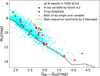 |
Fig. 1 Colour-magnitude diagram for M dwarfs in the TESS SCVZ (cyan) with the two samples defined in Sect. 3.4 highlighted in green (count rate ≥ 1 cts s−1) and red (count rate ratio between eRASS2 and eRASS3 ≥ 2 cts s−1). The overlap between the two samples are marked in orange. Overplotted is the main sequence isochrone (black) from the table ‘A Modern Mean Dwarf Stellar Color and Effective Temperature Sequence’ by E. Mamajek (https://www.pas.rochester.edu/~emamajek/EEM_dwarf_UBVIJHK_colors_Teff.txt). |
3.2 Selection of M dwarfs in the TESS SCVZ
We used Gaia DR2 coordinates and colours and employed the following criteria to identify M dwarfs within the TESS SCVZ:
- 1.
Colour selection: we identified M dwarfs on the basis of GBP – GRP colour, obtained from the integrated Gaia mean apparent magnitudes measured with the blue and red photometer, BP and RP, respectively4. We made our colour selection using the table ‘A Modern Mean Dwarf Stellar colour and Effective Temperature Sequence’ by E.Mamajek5, according to which dwarfs of SpT M0V and later have BP-RP ≥ 1.815 mag.
- 2.
Exclusion of giant stars: following Magaudda et al. (2022b), we used the absolute Gaia magnitude, MG, with the criterion MG ≥ 5.0 mag to exclude suspected giant stars from our selection.
- 3.
SCVZ stars: we specifically selected stars in the SCVZ limiting the ecliptic latitudes (b) to within 12° of the Southern ecliptic pole, that is b ≤ −78°.
A total of 874 stars within the examined sky area of 452.39 (deg2) met the aforementioned criteria. Figure 1 displays a Gaia colour-magnitude diagram (CMD) for these stars and Fig. 2 shows how they are distributed by their distances. In these figures we show the sample selected from TESS and Gaia as described above, and the subsample of it studied in this work. The latter one resulted from further downs election on the basis of eRASS data (see next section).
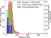 |
Fig. 2 Distribution of distances for the two subsamples that are X-ray brightest and the most X-ray variable defined in Sect. 3.4 as well as the entire M-dwarf sample in the TESS SCVZ described in Sect. 3.2. |
3.3 Search for eRASS X-ray counterparts
To identify those M dwarfs from the sample defined in Sect. 3.2 that had an eRASS X-ray detection we performed a match between Gaia coordinates and eRASS coordinates from the preliminary version of eRASS2 and eRASS3 catalogues produced by the eROSITA_DE consortium (all_e2_201221_poscorr_mpe_clean.fits and all_e3_210707_poscorr_mpe_clean.fits, respectively). The catalogues we used were the cleaned and position corrected catalogues (Brunner et al. 2022) processed using the eSASS pipeline version c946. These catalogues contain the merged source catalogues of each sky tile, with duplicates from overlapping sky tiles removed (‘cleaned’) and the coordinates of the sources boresight corrected (RA_CORR and DEC_CORR in the official catalogues). However, the stellar positions used for this match required correction for proper motion because most of the stars are located in proximity to the Sun (as shown in Fig. 2), and the Gaia-DR2 coordinates pertain to J2015.5, approximately 5 years prior to the eRASS surveys.
We extrapolated the optical positions of all stars to the mean observing date of both eRASS2 and eRASS3. The mean observing date epochs of eRASS2 and eRASS3 are 12 September 2020 and 16 March 2021, respectively, which corresponds to a time difference of 1961 and 2146 days between the middle of each of the two eRASS survey epochs and the Gaia-DR2 epoch. After proper motion correction to these two dates our target list was cross-referenced with the eRASS2 and eRASS3 catalogues using a match radius of 30 arcsec. Among the 874 M dwarfs, we find that 303 stars are listed in the eRASS2 catalogue, 293 stars are present in the eRASS3 catalogue, and 256 stars have detections in both the eRASS2 and eRASS3 catalogues.
3.4 X-ray brightest and most variable M dwarfs
In this work, we focused on a sub-sample of M dwarfs with high or strongly changing eRASS count rate. This warranted the best signal for our pilot study to quantify the relation between optical and X-ray variability. We defer the discussion of the X-ray and optical activity signatures of the full sample of M dwarfs in the TESS SCVZ that have TESS and eRASS data to a future work.
In order to further down-select our sample, and define the X-ray brightest and most variable M dwarfs from the list of 256 stars with both eRASS2 and eRASS3 detections, we applied the following criteria:
- 1.
Our selection of the stars with the highest photon statistics was based on the eRASS count rate in the 0.2–5.0 keV energy band (column ML_RATE_0 in the eRASS catalogues). We chose the stars with
 (1)
(1)
in at least one of the two eRASS surveys (i = 2, 3 for eRASS2 and eRASS3). For the 256 stars with both eRASS2 and eRASS3 detections, the median count rate error was 0.01 cts s−1. This criterion identified a total of seven stars as the X-ray brightest.
- 2.
In order to find the stars that showed the strongest variability between eRASS2 and eRASS3, we chose the stars with
 (2)
(2)
with i = 2,3 and j = 3,2. This ratio was associated with a median error of 0.2. This condition identified 23 stars as the most X-ray variable between eRASS2 and eRASS3.
The combination of the two criteria lead to the selection of 27 stars. Figure 3 displays ML_RATE_0 from eRASS2 versus eRASS3 in which the selection criteria can be observed. All the M dwarfs in the TESS SCVZ are marked in blue, the X-ray brightest stars from Eq. (1) in red, the most X-ray variable stars from Eq. (2) in green and stars that fulfil both criteria in lime. The diagonal where stars with no change in brightness between the two eRASS surveys lie is drawn in black and the dashed lines indicate a factor two change in X-ray brightness between the two surveys. We note that the individual errors on the count rates were not considered in the selection, and for some of the stars emerging from the second of the above criteria their error bar crosses the dashed lines in Fig. 4. We found this to be acceptable, as for this pilot study the aim is not to assert that the sample consists of inherently bright or variable stars but to maximize the chance to find flares with a reasonable signal so that they can be studied.
In the Gaia CMD of Fig. 1, we overlaid the final sample on the full sample of M dwarfs in the SCVZ from our master table defined in Sect. 3.2. It illustrates that the stars are evenly distributed across the M-dwarf spectral sequence, and in particular among the M dwarfs in the TESS SCVZ. The distance distribution of the X-ray brightest and most variable stars together with all M dwarfs in the TESS SCVZ is shown in Fig. 2, showing that the stars tend to be nearby, mostly within 100 pc. This is because predominantly bright and nearby M dwarfs were selected for the TESS two-minute target lists, and an additional preference for stars at short distance from our eRASS selection criteria.
Each of the 27 X-ray selected stars has, by definition of the sample, one light curve each for eRASS2 and eRASS3. This resulted in a total of 54 eRASS light curves. However, not all of the TESS light curves corresponding to the eRASS observations were available in the MAST database. Moreover, some of the light curves, both from TESS and eRASS, lacked simultaneous coverage due to the TESS LAHO gaps (see Sect. 2.1), and in some cases discarded data within the TESS light curve because of failed quality checks. Ultimately, there were 42 eRASS light curves from 25 stars that met the criteria of being the brightest or most variable M dwarfs in X-rays and also having simultaneous TESS two-minute data. This database serves as the basis for the remainder of this paper.
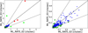 |
Fig. 3 Variation of the X-ray count rate in the 0.2–5.0 ke V band between eRASS2 and eRASS3 for the M dwarfs in the TESS SCVZ. Left panel – all stars, right panel – zoom into the low count rate region. The lines denote equal count rates in both surveys (solid) and differences of a factor two (dashed). The X-ray brightest stars (Eq. (1)) are high-lighted in red, the most X-ray variable (Eq. (2)) in green and stars that fulfil both critera in lime. See Sect. 3.4 for details. |
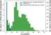 |
Fig. 4 Distribution of rotation periods of our final M-dwarf sample of the X-ray brightest or most X-ray variable stars (blue) and of the sample of all M dwarfs detected in a 10-month observational period of the 4-year Kepler mission from McQuillan et al. (2013) (green). |
4 Stellar parameters from Gaia, eRASS, and 2 MASS catalogues
We obtained stellar parameters for the 25 stars of our final sample using data from the Gaia, 2 MASS and eRASS catalogues. We retrieved the 2 MASS data for our stars directly from the Gaia archive using the Gaia-DR2 SOURCE_ID, as the cross match between 2MASS and Gaia-DR2 catalogues has been pre-computed by the Gaia DPAC (Data Processing and Analysis Consortium). We also obtained the Johnson–Kron–Cousin V from Gaia magnitudes GBP and GRP using the relation from Jao et al. (2018). We used the empirical relations from Mann et al. (2015) to calculate the stellar radii and masses from the absolute Ks-band magnitude, MKs, the effective temperatures (Teff) as an average of the values found individually using Bp – Rp with J – H and V with J – H, and bolometric corrections to Gaia magnitudes, which we then used to calculate bolometric luminosities, Lbol. We calculated the time-averaged observed X-ray flux (〈Fx,obs〉) from the mean count rate (ML_RATE_O) provided in the eRASS catalogues using a conversion factor of 7.81 × 10⁻¹³ erg cts−1 cm−2 derived by Magaudda et al. (2022b) from eROSITA spectra of M dwarfs. We used the stellar radii and the distances from Gaia parallaxes to calculate the average X-ray luminosity (〈LX〉) and X-ray surface flux (〈Fx,surf〉) of the given eROSITA survey. The values for all these parameters for the 25 stars are available through the catalogues (available at the CDS). The columns of these catalogues are described in Appendix A.1 and B.1.
5 Analysis of eRASS light curves
5.1 eRASS data extraction
We extracted the eRASS light curves using the eSAS-Susers_211214 software release (Brunner et al. 2022) for our sources in such a way that they were binned regularly with a bin size of 1 eRODay and any empty bins were discarded (i.e. bins having zero fractional exposure). In addition, only the bins with fractional exposure fracexp ≥ 0.00005 are included as bins with low fractional exposure have large error values. The above cutoff value for fracexp was chosen as it eliminated bins with a significantly smaller fractional exposure than the rest of the data points in the light curve. As described in Sect. 2.2, as the eROSITA scans of the great circles progress, a given source moves in and out of the telescopes’ FOV. This means that the fracexp tends to be lowest when the source is at the edge of the FOV, which corresponds to the beginning and end of the light curve.
5.2 Definition of eRASS quiescent level
In this paper, variability in the eRASS light curves is quantified by first defining a quiescent count rate, Rqui, and then marking the light curve bins that are significantly above it, which we interpret as being part of flares. To do this, the eRASS count rates are divided into equally sized bins and bin size is chosen as the maximum of two optimum bin size estimators, the Freedman Diaconis Estimator (Freedman & Diaconis 1981) and the Sturges estimator (e.g. Scott 2009) implemented using the Numpy package in Python (Harris et al. 2020). The X-ray quiescent level (purple in the example shown in Fig. 5) is defined using the two criteria described in the following.
We used the bin with the lowest count rate that had at least two data points to define the quiescent level as its upper edge, that is the boundary between this bin and the next (higher) one. If no such bin existed, we used the overall lowest count rate bin, even if it comprised only one or two data points. We prioritized bins with more than two data points, because the lowest count rates are sometimes negative and have large error values associated with them. This occurs for stars that are very faint, comparable to, or even fainter than the background. Secondly, we required that the quiescent levels had their upper boundaries above zero cts s−1. If this was not met by the bin selected with the first criterion, we used the upper boundary of the next highest count rate bin (i.e. the bin above it) as Rqui value. Similar to the first criterion, this is necessary as for some light curves the lowest count rate bin has only data points with ML_RATE_O < 0 cts s−1, and a negative quiescent level is unphysical. The quiescent count rates we obtained from each eRASS light curve of our targets, Rqui,eRASS2 and Rqui,eRASS3, along with the mean of the two values Rqui,mean and the standard deviation (Rqui,std.dev) between them are presented in Table 1.
TIC ID, quiescent rate from eRASS 2 (Rqui,eRASS2), eRASS 3 (Rqui,eRASS3), the mean quiescent rate (Rqui,mean), and the standard deviation (Rqui,std,dev) from the two surveys in cts s−1, eRASS duty cycle of eRASS 2 (vx,DC,eRASS2), eRASS 3 (vx,DC,eRASS3), the mean eRASS duty cycle (vx,DC,mean), and the standard deviation (vx,DC,std,dev) of the two eRASS surveys.
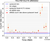 |
Fig. 5 Example of an eRASS light curve (the M dwarf TIC278731274 observed in eRASS2) demonstrating the definition of the quiescent count rate level, Rqui, and the selection of variable light curve bins (namely eROdays significantly above Rqui; see text in Sects. 5.2 and 5.3) |
5.3 eRASS duty cycle of variability
The bins which are located significantly above the quiescent level were considered to be ascribed to variability of the star. These bins are marked in red in Fig. 5. We defined ‘significantly above the quiescent level’ as an upward excursion of at least 1 σ. That is, the lower bound of the 1σ uncertainty on the count rate must lie above the quiescent level, Rqui.
Flare counting is difficult in eRASS light curves because the gaps between subsequent data-taking intervals (eROdays) of 4h are of the order of the duration of or even longer than an X-ray flare while the individual visits to the source are of the order of 100 s, thus capturing only a snapshot in the evolution of a flare. To quantify the overall level of variability in eRASS light curves, we defined a duty cycle (νx,DC) for the X-ray variability as the ratio of the number of bins corresponding to eROdays significantly above the quiescent level (Nx,var) to the total number of bins in the light curve (Nx,total):
 (3)
(3)
We computed the eRASS duty cycle individually for the light curves only within the time intervals that had TESS observations. The eRASS duty cycle of the stars obtained from the light curves of the two surveys individually, (νx,DC,eRASS2 and vx,DC,eRASS3), along with the mean of the two values (vx,DC,mean) and their standard deviation (νx,DC,stddev) are provided for all stars in Table 1.
6 Analysis of TESS light curves
The two-minute TESS light curves are of the form Pre-search Data Conditioning Simple Aperture Photometry (PDCSAP) flux versus TIME. PDCSAP flux is used as long-term trends have been removed from the data and it tends to be cleaner and have fewer systematic errors than Simple Aperture Photometry (SAP) flux. TIME is in units of Barycentric Julian Date (BJD)-2457000.0. The light curves in this work have been normalized by us for analysis by dividing the values of all PDCSAP flux data points by their mean flux value. We applied our rotation and flare detection code to the normalized TESS light curves. Specifically, in this work we use the Python version which mainly consists of a translation of the IDL code used in our previous works (Stelzer et al. 2016, 2022a; Raetz et al. 2020).
Rotation periods and optical variability diagnostics derived from TESS light curves.
6.1 Detection of rotation and flares
The rotation period of the star can be obtained by analysing the periodic modulation of optical light curves that arises from the presence of photospheric star spots. The amplitude of the variability provides information about the amount and distribution of spots on the surface. Our rotation and flare detection code uses the Lomb-Scargle periodogram from the Python package Astropy (Astropy Collaboration 2013, 2018, 2022) for the search of the rotation signal. The Lomb-Scargle periodogram (Lomb 1976; Scargle 1982) is a tool to find the periodicity of (unevenly) spaced observations (see also VanderPlas 2018). We calculated the Lomb-Scargle periodogram separately for each of the TESS light curves from the full light curves of the sectors that overlap with the times of eRASS2 and eRASS3 observations of our targets.
As a baseline we adopted the highest peak in the periodogram as Prot. To validate these periods we required that (i) a clear signal was seen in the phase-folded light curve and (ii) the highest peak had at least two times as much power as the second highest peak. We kept two period values that did not fulfil criterion (ii), because the second highest peak was at one-half the period of the highest peak and the light curve appeared ‘double-dipped’ (TIC 33866201 in eRASS2 epoch, TIC 220473309 in eRASS2 epoch). These cases are usually ascribed to a spot pattern that changed from spots dominating one hemisphere to a more even distribution in terms of stellar longitude (McQuillan et al. 2013). In one case (TIC 278735797), a clear periodic signal was present at both epochs with the value for Prot differing by about a factor two. Here, visual inspection showed that the light curve with the detection of the shorter period showed a more complex modulation. Since it is not essential for our study whether we have detected the rotation period in one or two epochs, we ignored the shorter Prot value from the complex light curve at eRASS3 epoch for this star.
To summarize, we were able to determine Prot for 18 of 25 stars. All periods, referred to as Prot,e2 and Prot,e3 respectively, are presented in Table 2. With the exception of TIC 278735797 discussed above, if two periods were found for a given star from the two epochs, the values were consistent with each other.
The light curve with rotational modulation signal subtracted, which is obtained by applying boxcar smoothing and subsequently subtracting the smoothed curve over three iterations, provided a ‘flattened’ light curve from which the upward outliers could be identified as white light flare signatures or ‘flare candidates’. The boxcar width for the smoothing was adapted to the previously determined rotation period. Specifically, values of 80, 60 and 40 data points were used for the three successive iterations for light curves with Prot ≤ 3.3 days, and boxcar widths of 150, 100 and 40 were used for Prot > 3.3 days. From this flare signal, the rise and decay time of white light emission could be found as well as the flare energy emitted in white light by integrating over the flare light curve. The above procedure is explained in detail in Stelzer et al. (2016, 2022a), Raetz et al. (2020). The validation of the flare candidates includes the use of an empirical flare template from Davenport et al. (2014), according to which, valid flares must satisfy the following criteria, as described by Raetz et al. (2020), which we reiterate here:
- 1.
The flare shall not be close to a data gap, where a ‘gap’ is defined here as a timespan of at least 10 min without data and events within ±10 min of the gap edges are not considered.
- 2.
The ratio of the maximum (or peak) of the flare to the minimum of the flare f(peak) : f(minimum) must be at least 2:1
- 3.
The rise time must be shorter than the decay time
- 4.
The peak of the flare must not be the first or last point of the light curve
- 5.
The flare model must fit better than a linear model
We calculated the TESS flare energies in ergs (also detailed in e.g. Stelzer et al. 2016, 2022a, Raetz et al. 2020, which we reiterate here) by multiplying the equivalent duration (ED), which is defined as the area under the flare light curve (e.g. Hunt-Walker et al. 2012), with the quiescent TESS luminosity Lqui,T. The ED has units of seconds, as we integratied over the dimensionless normalized light curve. Lqui,T is determined from the quiescent flux in the TESS band (Fqui,T) and the Gaia distances. Fqui,T is calculated from the zeropoint ZPTESS = 1.34 × 10⁻⁹ erg cm−2 s−1 Å−1, the TESS magnitude (T) and the filter bandwidth Weff = 3898.68 Å as Fqui,T = ZPTESS · 10−0.4 · T · Weff. ZPTESS and Weff were obtained from the website of the Spanish Virtual Observatory6.
6.2 TESS variability diagnostics
For the sake of comparison with the X-ray data, in our study of optical variability we considered only that portion of the TESS light curves that corresponded to the epoch and duration of the eRASS visits to the respective star. We defined two parameters that describe the frequency of flares in TESS light curves. First, the TESS flare rate (νo,f) for each light curve, which was the number of validated flares that were detected in the light curve (No,f) normalized by the length of the light curve in days (∆to) excluding data gaps:
![Mathematical equation: ${v_{{\rm{o}},{\rm{f}}}}\left[ {{{\rm{d}}^{ - 1}}} \right] = {{{{\rm{N}}_{{\rm{o}},{\rm{f}}}}} \over {{\rm{\Delta }}{{\rm{t}}_{\rm{o}}}}}.$](/articles/aa/full_html/2024/08/aa49405-24/aa49405-24-eq4.png) (4)
(4)
This parameter is the standard way of defining flare rates, see for example, Stelzer et al. (2022a).
Secondly, a duty cycle was defined for TESS light curves, νo,DC, analogously to the eRASS duty cycle, as the ratio of the total number of flare bins in the light curve (Nf pts) to the total number of bins in the TESS light curve (Nall pts):
 (5)
(5)
As for the X-ray duty cycle, we have computed the optical duty cycle individually for the time intervals in the light curves that are covered by the two eRASS surveys (vo,DC,eRASS2 and νo,DC,eRASS3). In some of our analyses, we used the mean of the optical (TESS) duty cycle νo,DC,mean, which is the average of vo,DC,eRASS2 and vo,DC,eRASS3. As a measure for the uncertainty of vo,DC we used the standard deviation obtained from the two values. The flare rates and duty cycles are presented in Table 2.
7 Results
7.1 Rotation period and X-ray activity
The distribution of Prot values in our sample of 25 M dwarfs is shown in Fig. 4 together with a large sample of M dwarfs observed with the Kepler mission (see below). All stars in the sample for which a period could be detected were fast rotators with the highest value being Prot ~ 8.6 days. This can be explained by the fact that active stars have shorter rotation periods, and the sub-sample of M dwarfs used in the analysis was specifically chosen as highly X-ray-active (either by high count rate or strong variability in eRASS), as specified in Sect. 3.4. This sample is therefore biased towards active and fast rotating stars in comparison to, for example, M dwarfs detected by the Kepler space mission whose properties were studied amongst others by McQuillan et al. (2013). Figure 4 illustrates the two period distributions, from which the bias in our sample towards fast rotators becomes evident. On the other hand, periods longer than 15 days (roughly half the time-span of a TESS sector light curve) could not be confidently measured, introducing another bias towards fast-rotating stars into our sample.
With their short periods, we found our stars to lie in the saturated regime of the rotation-activity relation, as can be seen from Fig. 6. The range of Lx/Lbol covered by our sample is in agreement with the spread of the saturation level observed in the so far largest sample of M dwarfs examined for the rotation-activity connection (Magaudda et al. 2020, 2022b). As compared to representations based on Lx, the use of the Lx/Lbol ratio removed most of the mass-dependence of activity (except for a possible residual effect; see e.g. Reiners et al. 2014; Magaudda et al. 2022a). The origin of the remaining spread of the saturated level of about one dex is not fully understood. Our data suggests that it is determined by variability together with a residual mass-dependence. The mean log (Lx/Lbol) value of our targets shown in Fig. 6 is −3.13 with a standard deviation of 0.37, and similar values are obtained for our full sample including the stars without rotation period measurement.
7.2 Optical flare frequency distribution
We computed for each of the 22 stars from our sample that displayed optical flares its cumulative flare frequency distribution (FFD) from the TESS light curves of the two sectors that overlap with eRASS. The FFDs were calculated by combining the flare energies obtained from both sector’s light curve into one FFD per star. The FFDs of our stars are shown in Fig. 7, from which it is evident that our sample spans a large range in flare activity.
The most important parameter of FFDs is the slope of a power law fit, which is crucial for an assessment of the importance of nano-flare heating (e.g. Hudson 1991; Veronig et al. 2002). At low energies FFDs are known to flatten because small-amplitude flares are not detectable. The minimum detectable flare energy, which depends on the noise level of the light curve, can be determined by simulations. A quantitative analysis of the TESS FFDs of our targets is not within the scope of this paper, as systematic studies of FFDs have been carried out on larger samples of M dwarfs (e.g. Günther et al. 2020; Raetz et al. 2020). Therefore, we have not computed the slopes and completeness thresholds of our FFDs.
In Fig. 7, we merely display the FFDs of our sample in comparison to a sample of nearby M dwarfs studied by Stelzer et al. (2022a). These latter ones are the 12 stars from the catalog of Kaltenegger et al. (2019) for which Stelzer et al. (2022a) could determine the rotation period from the TESS light curves of all sectors in which the star was observed. Their Prot values range between 0.3 and 4 days, comparable to the periods of the stars from our combined eRASS/TESS sample. Yet, as can be seen from Fig. 7, our sample is on average characterized by higher optical flare frequencies. This confirms the bias towards strongly active stars introduced by our X-ray selection criteria.
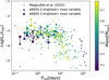 |
Fig. 6 Relation between X-ray activity and rotation of our sample (large triangles and squares are for eRASS2 and eRASS3, respectively) compared to the M-dwarf samples from Magaudda et al. (2020, 2022b) (dots). The stars are colour-coded by mass and lines connect the two epochs for a given star from our sample. |
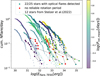 |
Fig. 7 Optical flare frequency distributions of the 22 targets with flares detected in the TESS light curves of the sectors overlapping with eRASS (circles). For comparison the FFDs for the fast rotating M dwarfs from the catalog by Kaltenegger et al. (2019) that were studied by Stelzer et al. (2022a) are shown ( small crosses). |
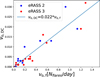 |
Fig. 8 TESS duty cycle νo,DC versus TESS flare rate νo,f, along with a linear fit to the data (blue line). For each star, the TESS results from the data overlapping in time with the eRASS2 and eRASS3 light curve, respectively, are distinguished by different colours. |
7.3 Global X-ray and optical variability diagnostics
To compare the different information content of the TESS and eRASS light curves that derived from the very different observing cadence of the two surveys, we have defined in Sects. 5.3 and 6.2 global variability diagnostics. These represent the overall level of variability of a given light curve as a single number. Here we examine relations between these different variability diagnostics.
In particular, for both eRASS and TESS we have defined the duty cycle of variability in the same way, as fraction of time the star was in a ‘high-state’. We compare the optical (TESS) duty cycle (vo,DC) and optical flare rate (νo,f) to each other. Hereby, we evaluate the parameters for the two timespans corresponding to the eRASS2 and eRASS3 observation of the stars individually. Fig. 8 demonstrates that the optical duty cycle correlates very well with the optical flare frequency. The Pearson’s correlation coefficient between νo,DC and νo,f is 0.934 with a p-value of 1.22 × 10⁻¹⁷. We also performed a linear fit between νo,DC and νo,f, and found that the line νo,DC = 0.022*νo,f fit the data best. This high level of correlation was not unexpected, as more flares in the light curve means that the overall time the star has spent at elevated level of brightness is higher. More precisely, the key difference between the TESS flare frequency and the TESS duty cycle is that the latter is a function of both the flare rate as well as the duration of the flares. Since the flare frequency scales with the flare energy (Sect. 7.2), and the flare energy is determined by both the amplitude and the duration of the flare, the flare frequency is higher for events that last longer. Hence, the duty cycle increases as the frequency of flares increases. In the following, we use the TESS duty cycle as a proxy for the optical variability because this parameter is formally equivalent to the X-ray duty cycle that we have defined for eRASS light curves.
The mean TESS duty cycle vo,DC,mean is plotted against the mean eRASS duty cycle vx,DC,mean in Fig. 9. The Pearson’s coefficient is 0.578 with a p-value of 0.01, and the Spearman’s rank correlation coefficient is 0.638 with a p-value of 0.003. The optical and the X-ray duty cycles, thus, show a significant correlation. The still rather significant scatter in the relation might indicate that a range of multi-wavelength energetics is associated with flares. The values for the TESS duty cycles were much lower than those of the eRASS duty cycles, which is likely a combination of the different data cadences of the two surveys and the different intrinsic duration of optical and X-ray events, as mentioned above. The eRASS duty cycle could not directly be interpreted as a flare rate, because (a) flares could be missed in the 4 h gaps between two eROdays and (b) X-ray flares can last several hours such that the duty cycle is not equivalent to flare counting.
We examine the relation between the activity duty cycles and the rotation period in Fig. 10. Here, each star is represented by the black line connecting the duty cycles and rotation periods from the time interval of eRASS2 and eRASS3 observations. As mentioned previously, the TESS duty cycle was calculated only for the time of overlap between TESS and eRASS observations. We observed a trend of high duty cycles, both in X-rays and in optical, occurring predominantly on fast rotators (Prot ≲ 2 days). However, the star with the highest value of vo,DC had the longest period. This star had a very prominent double-humped TESS light curve, which could imply that it was strongly spotted. A sample with a broader range of Prot would be needed to establish an activity-rotation relation for the duty cycles, as other studies have shown a bimodal distribution separating active from inactive stars at a value of Prot ~ 10 days (e.g. Wright et al. 2011; Raetz et al. 2020; Magaudda et al. 2022b).
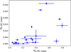 |
Fig. 9 TESS mean duty cycle versus eRASS mean duty cycle, with the standard deviations between the values from the two eRASS epochs represented as uncertainties. |
7.4 Association of optical flares to X-ray flares
The association of the eRASS X-ray variability with the distinct optical flares seen with TESS was difficult due to the long data gaps (of 4 h) between individual X-ray exposures during the eRASS. To identify joint optical and X-ray variability, we examined for each ‘X-ray flare data point’ (XFDP), defined as a light curve bin significantly above the quiescent level (red in Fig. 5; see Sect. 5.2), whether there was an optical flare preceding it by at most 2 h, equivalent to 1/2 eROday.
To overcome the problem of the low cadence of the eRASS light curves, we used information about the typical duration of stellar flares and the timing between the optical and X-ray component of a flare. In the standard flare scenario (Cargill & Priest 1983; Benz 2017), a time lag is expected between the optical and X-ray flare peak. In fact, the time difference between the peak of the optical and X-ray brightness in a giant flare on the M dwarf AD Leo was ≈300 s (Stelzer et al. 2022b), and similar delays have been observed in other stellar flares (e.g. Katsova et al. 2002; Stelzer et al. 2006) as well as solar flares (Castellanos Durán & Kleint 2020). The typical optical/X-ray time lag of a flare is, thus, much shorter than one eROday, the cadence between subsequent bins in the eRASS light curves. Therefore, optical flares are expected to be found around some XFDPs in a time window that is a fraction of 1 eROday. Other XFDPs are expected to have no optical counterpart within an eROday as the X-ray flare is part of the ‘gradual’ phase of flares (Hudson 2011) and its duration is far longer than that of the optical flare which belongs to the ‘impulsive’ phase. This solar flare morphology has been confirmed for events on other stars, see for example, Stelzer et al. (2022b).
To ensure that we had not missed any joint optical/X-ray flare events, we searched all XFDPs for TESS flares that preceded them by at most 1/2 eROday, centred on the time within the eROday when eROSITA observed the star. This required a different binning of the eRASS light curves as compared to the one used above in the standard analysis. The eRASS light curves used above were binned with a bin size of 4 h, which is the cadence of eROSITA visits to a given sky position, as explained in Sect. 5. However, the actual exposure on the source during this 4 h timespan is only of the order of 40 s, meaning that most of an 4 h-bin holds no data. We did not know at which time within the 4 h interval eROSITA actually took data of the source. In other words, in a light curve binned with the 4 h (alias 1 eROday) cadence every data point has a timing uncertainty of 4 h. Given the typical duration of optical flares of ≲10 min (Hawley et al. 2014; Namekata et al. 2017) and the typical time lapse between optical and X-ray flare peaks of ~5min (see above), such a high uncertainty in the timing makes an association between X-ray and optical flares difficult. To recover X-ray timing information, the binsize must be of the order of the net on-source time within an eRODay, but this information is not trivial to extract. We, therefore, produced a second set of eRASS light curves, binned into 40 s intervals. Evidently, this produces many empty bins but it improves the time-resolution by a factor 360. An example of the improved accuracy in timing is illustrated in Fig. 11 which shows the same light curve binned with the method just described together with the light curve binned at intervals of one eRODay. A systematic shift of the two light curves by roughly 1/2 eRODay is seen in this case. Generally, time shifts between the two binnings range from 1/8 eRODays to 1/2 eRODay for our stars which means that the light curve with the coarse (1 eRODay) binning is far from providing the best possible estimate for the peak time of the flare. The drawback of eRASS light curves with small bin size is that it happens that the short on-target time during one eRASS visit of the source is split onto two 40 s bins. This way of binning the eRASS data, thus, may produce some bins with extremely short exposure that have huge errors on the count rate. Since these bins hold only a minor fraction of the counts, excluding them from the analysis does not lead to a major loss of data. For the representation in Fig. 11 as well as for the further analysis, we, thus, removed bins with fractional exposure FRACEXP < 0.01 and we combined, in the remaining light curve, the bins which were very close in time (i.e. belonging to a single eRODay) by averaging their time, rate and errors.
With this procedure, we again had one bin per eROday in the light curve, as before in the standard analysis. However, this bin was now positioned at the actual time when eROSITA observed the star. This means, that in these new eRASS light curves we now knew the time of observation with 40 s precision, and we could proceed towards our goal of searching for the optical counterpart of X-ray flares. In Fig. 12 we show an example of the outcome of this search: The XFDPs are marked in red like in Fig. 5. The time windows of 1/2 eRODay around eROSITA X-ray flare bins that are preceded by TESS flare bins are marked with blue dashed lines, and these XFDPs are highlighted as green squares. The respective TESS flares occurring up to half an eROday before and after an X-ray flare data point are marked in dark blue.
To quantitatively evaluate our search for joint optical/X-ray variability, we examined what fraction of all XFDPs in a given eRASS light curve had a TESS flare preceding it within 1/2 eRODay before the XFDP The number of XFDPs with a corresponding optical flare found in this interval is plotted against the total number of XFDPs in the eRASS light curve in Fig. 13. First, we noticed that a high number of X-ray flare bins have no optical event associated with them. This might occur for the following reasons: (i) the XFDP could have been part of the advanced decay phase of the X-ray flare. As discussed above, X-ray flares last hours to days, whereas optical flares decay on timescales of a few minutes. Fig. 12 shows several such events in which the X-ray flare probably lasted for several eRODays. (ii) There was a true absence of an optical counterpart to the X-ray event. There have, indeed, been instances from the solar literature where X-ray flares have been observed with no optical counterpart (Namekata et al. 2020). Overall, both numbers appear to be correlated. The Pearson’s coefficient for the correlation of the two parameters is 0.771 with a p-value of 3.75e–11. This means that for light curves with many X-ray flares occurring, the chances of finding them occurring together with optical flares are high.
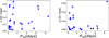 |
Fig. 10 X-ray duty cycle vx,DC,mean versus rotation period (left) and optical duty cycle vo,DC,mean versus rotation period (right). Lines connect the two epochs for a given star. |
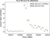 |
Fig. 11 Example of an eRASS light curved binned at 40 s, with bins close in time being combined (orange) and the same light curve binned at 1 eRODay. For this example the time-shift between the two light curves is roughly 2 h or 1/2 eRODay. |
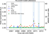 |
Fig. 12 Example of a flattened TESS light curve and eRASS light curve for TIC 220473309 observed during the eRASS2 epoch of the star. The eRASS data points significantly above the quiescent level (purple-shaded area), also named as the ‘X-ray flare data points’ (XFDPs), are marked in red. The TESS flare data points are marked in dark blue. XFDPs around which TESS flares were found are marked as green squares, and the vertical bins of width 1 eROday in which they lie are marked with dashed blue lines. |
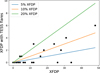 |
Fig. 13 XFDPs that are preceded by TESS flares versus all XFDPs per eRASS light curve. The orange, blue and green lines denote 20%, 10% and 5% of XFDPs that are preceded by TESS flares, respectively. |
7.5 X-ray flare energetics
As discussed before, the low eRASS data cadence makes it difficult to quantify X-ray flares. Given a typical X-ray flare duration of one to a few hours, plausibly even a single individual XFDP which has ‘quiescent’ bins on both of its sides may represent a full-fledged flare, for which however both rise and decay phase cannot be constrained. To provide an (albeit coarse) estimate of the X-ray flare energies from the poorly sampled eRASS light curves we made inferences from solar data combined with the observed TESS flares to constrain the timing and flux of the peaks of the X-ray flares. Then, we performed an exponential fit starting with the estimated X-ray flare peak. Finally we derived the X-ray flare energy by integrating under the fit curve.
The analysis described in this section is carried out on all 58 detected TESS flares, irrespective of any evidence of X-ray flaring in the eRASS light curve surrounding the TESS event. We caution, that this analysis presents many severe approximations and assumptions as we detail in the following description of the procedure. Yet, as will be shown below it produces reasonable results.
7.5.1 Estimate of the X-ray flare peaks
We estimated the eRASS count rate of the (unobserved) X-ray flare peak of potential X-ray flares associated with TESS flares with the help of the empirical relation from Namekata et al. (2017) for solar flares between the GOES soft X-ray flux (Fpeak,GOEs) at the peak and the energy of the corresponding WLF (EWLF). We used the updated fit from Stelzer et al. (2022b) which includes data from the Nov 2022 Great Flare on the M dwarf AD Leo, and spans a much broader range of GOES peak flux and WLF energy than the solar flares alone. To be able to apply the EWLF – Fpeak, GOES relation, we first calculated the WLF energy of the TESS flare. Hereby we assumed the optical flare to be represented by blackbody emission at a constant temperature of Tf = 9000 K (as is typically observed for solar WLFs, Kretzschmar 2011). Then we followed Shibayama et al. (2013) to calculate the emitting area AF(t) (assumed to be variable along the event), and then we integrated the bolometric flare luminosity  ⋅ AF(t) over the flare light curve to find EWLF.· We find the WLF energy to be higher than the flare energy in the TESS band by a factor 5. Next, we obtained Fpeak,GOES from the above mentioned relation with EWLF.· The GOES flux is the flux of the flare peak observed at 1 AU from the source (namely the distance of the GOES satellites from the Sun). This must be translated into the peak flux observed from the star at Earth, by scaling with the star’s distance calculated from the Gaia parallax. The resulting value still refers to the GOES band (1.5–12.4 keV). The last step was to convert the flux from the GOES band into the eRASS band used for our light curves (0.2–5.0 keV) and obtain the corresponding count rate. To achieve this we used the Great X-ray Flare on AD Leo (Stelzer et al. 2022b) for which the peak flux was measured both in the eRASS and in the GOES band using XMM-Newton data, yielding an eRASS-to-GOES flux ratio of 1.8 (priv. comm., M. Caramazza). By applying this conversion factor to our data, we assumed that the relative flux distribution of the flare peak in different X-ray sub-bands is universal for all X-ray flares. Finally, we converted the flux in the eRASS band to count rate for use in our eRASS light curves. Here we applied the conversion factor 1.1 × 10⁻¹² erg cts−1 cm−2 calculated from eRASS data of Prox Cen which is to our knowledge the best representative of eROSITA flare data that has been analysed so far (Magaudda et al., in prep.).
The result of this approach is that we gained an additional data point for the X-ray light curve, representing the peak of the flare. An example of this is shown in Fig. 14. We fixed the position of the X-ray flare peak in time to 5 min after the TESS flare peak which is the typical time-delay between optical and X-ray peaks of solar and stellar flares (Castellanos Durán & Kleint 2020; Stelzer et al. 2022b). Evidently, the count rate of the X-ray flare peak estimated from the associated optical flare energy can be much higher than the highest observed eRASS flux. Similarly, the time of the X-ray flare peak inferred from the typical delay with respect to the associated optical flare can be significantly before the eROday with the highest count rate. It is, therefore, clear that the estimated energetics of the X-ray flare rely strongly on the assumptions made in deriving this ‘synthesized’ flare peak. This is explored in the next subsections.
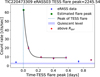 |
Fig. 14 eRASS3 light curve of TIC 220473309 illustrating our estimate of the X-ray flare peak (green data point) as explained in Sect. 7.5.1 and the exponential fit to the flare decay (black curve) described in Sect. 7.5.2. |
7.5.2 Fit of the X-ray flare profiles
Having an estimate of the peak time and count rate, we could fit a decaying exponential curve to the flare count rate (R) as  , where Rpost is the post-flare count rate, Rpeak is the estimated eRASS flare peak count rate, b = 1/τ is the decay coefficient, with τ the decay timescale, and txo is the start time of the X-ray flare. Rpeak and tx0 are not identical to the X-ray flare peak data point that we defined in Sect. 7.5.1. Rpeak is a free fit parameter, and txo is allowed to vary within a range of 5–10 min after the TESS flare peak.
The exponential fit is applied to the portion of the eRASS light curve starting 5 min after the peak of the optical flare (corresponding to the synthesized X-ray flare peak) and extending for 16 h. This limit on the time length of the fitted profile was appropriate for the following reasons: (1) Sixteen hours captured 5 data points (the synthesized peak and four subsequent eRO-Days) which is the minimum needed for fitting as imposed by our 4-parameter fit function, (2) by-eye inspection revealed that typically after 16 h, flares are either well into its decay and flattens out or a new flare starts. We can not rule out that this time-interval comprises subsequent variability not directly related to the X-ray counterpart of the optical flare. Indeed, if the flare decays back to the quiescent level, Rpost should be identical to Rqui defined in Sect. 5.2. However, in practice the fitted post-flare count rate is usually different from the quiescent count rate either because the corona remains in an elevated brightness after the flare (see e.g. the Great Flare on AD Leo; Stelzer et al. 2022b) or because the low number of eRASS bins does not fully constrain the decay or because subsequent flaring activity is overlaid on the first event.
For the 58 TESS flares from which the synthetic eRASS flare peak was estimated, we identified 17 X-ray flares by eye, for which the exponential decay fit the X-ray flare light curve relatively well. The X-ray light curves and the exponential fits of these events are presented in Appendix C.1. The stars TIC 150359500 and TIC 278731274 present TESS flares with particularly strong eRASS variability that, however, could not be fit with the exponential model. These peculiar flares are discussed in Sect. 7.5.4.
7.5.3 X-ray flare energies and comparison to optical flare energies
Going one step further, we could estimate the energy of the X-ray flare (Ef,x) from the profile of the exponential fit. Flare energies are commonly calculated by multiplying the quiescent luminosity with the integral over the light curve that was before normalized to quiescence, as described in Sect. 6.1 for the TESS flares. Applying this to the eROSITA X-ray light curves, posits the question of the appropriate quiescent count rate. As mentioned above, for a quiet light curve with individual flares superposed this should be the count rate Rqui determined in Sect. 5.2. However, Fig. 14 and Appendix C.1 show that this low count rate level is often not reached after the X-ray flare. We, therefore performed the calculation of Ef,x for two values of the ‘quiescent’ count rate, Rqui and R0. The latter is the last count rate of our fitted curves representing the flattened portion of the decay, that is, the count rate at 16h after the TESS flare peak.
The calculation of Ef,x was done as follows, separately for both versions of the ‘quiescent’ emission level. We first normalized the count rates of all light curve bins that have participated in the fit to the ‘quiescent’ count rate, and then we subtracted the normalized ‘quiescent’ count rate, which is equal to 1. This way we obtained a ‘flare-only’ light curve. We integrated under this curve to obtain the ED which has units of seconds as we are integrating over the dimensionless normalized curve. The X-ray flare energy, Ef,x was found by multiplying the ED with the luminosity obtained from the count rate Rqui or R0 (for the two versions) after applying the ‘quiescent’ rate-to-flux conversion factor from Magaudda et al. (2022b) (see Sect. 4) and the Gaia distance of the star.
In Fig. 15, we compare the resulting values of Ef,x with the energies from their optical counterparts found with TESS, Ef,TESS (see Sect. 6.1) for both assumptions of the quiescent level, Rqui in red and R0 in green. The Pearson’s correlation coefficient between log(Ex,f) and log(Ef,TESS) was found to be 0.907 with a p-value of 1.396e–8 for the exponential decays normalized to Rqui, and 0.839 with a p-value of 2.03e–6 for the exponential decays normalized to R0, demonstrating that for both assumptions on the post-flare count rate the optical and X-ray flare energies are well correlated.
When compared to the small sample of joint X-ray and optical flares on M dwarfs presented in the previous literature (black in Fig. 15) our X-ray flares appear overluminous with respect to the corresponding optical flares. This could be the result of the many severe assumptions made in Sect. 7.5.1 to constrain the X-ray counterpart of the TESS flares. While locating the X-ray flare peak time and flux with help of the TESS flare on the basis of earlier solar and stellar flare observations by Namekata et al. (2017) and Stelzer et al. (2022b) appears solid, we observe that in many cases this synthesized flare peak exceeds the highest count rate observed in the aftermath of the TESS flare by high factors (see Fig. C.1). This may lead to an overestimation of Ef,x. On the other hand, X-ray flares usually decay slower than an exponential, such that under this aspect our Ef,x values might be underestimated. As Fig. 15 shows our distribution of flares to be located above that of the joint optical/X-ray flares presented in the literature, we suspect that our X-ray peak flux estimates are too high.
Sanity checks on the X-ray flare energies. Given the well founded, but still strongly hypothetical tie to the optical flare imposed on the X-ray flare in our procedure, we tested three modifications to our analysis. We computed again, for each of the three modifications, the X-ray flare energies inferred and compared them with the original result from Fig. 15.
First, we repeated the fitting described above after arbitrarily scaling down the inferred flare peak (green ‘data’ point in Fig. 14) by a factor two in count rate. In Fig. 16 we compare the new values for Ef,x with the optical flare energies, displaying as well the earlier result. We show only the results where Ef,x was evaluated with respect to the last fitted data point (R0), because – as explained above – many flares seem not to decay all the way to Rqui and the corresponding values of Ef,x are, therefore, too high. The down-scaling of the X-ray flare peak yielded on average only slightly lower values of Ef,x for a given optical flare.
Secondly, we changed the flux at the inferred flare peak in the opposite direction, scaling upwards by a factor two with respect to the original value. This is motivated by a potential uncertainty in the eRASS-to-GOES flux conversion. The AD Leo flare we used to compute the conversion factor of 1.8 (see Sect. 7.5.1) had a temperature of 3.2 keV around its peak (Stelzer et al. 2022b). From two flares of somewhat lower energy on Proxima Centauri, 2.5 × 1031 erg and 1.4 × 1032 erg respectively, we measured peak temperatures of around 1 keV and 1 .3 keV, and the eRASS-to-GOES flux ratios of these events are ≈5 and 4 respectively (Magaudda et al, in prep.). The up-scaling of the X-ray flare peak yielded on average similar values of Ef,x, some only slightly higher, for a given optical flare.
Finally, we completely omitted the synthetic X-ray flare peak and evaluated the X-ray flare energy by integrating under the exponential fits to the X-ray flare light curves starting only from the first eRASS data point after the TESS flare. For this test, we used the exponential fits obtained with the original, un-scaled synthetic X-ray flare peak. We found that the resulting Ef,x values are up to one order of magnitude lower than those obtained by including the synthetic flare peak.
Overall, we found for all three sanity checks, that the positive correlation between optical and X-ray flare energies remains unchanged. Considering that the time lag of the first eROSITA data point after the TESS flare peak is often a large fraction of an eRODay (which is 4 h) and such a large time difference between optical and X-ray flare is unexpected, the last estimate that does not consider the information from the optical event appears as the least realistic and likely underestimates the true X-ray flare energies. From visual inspection it is not evident which of the three versions of the synthetic X-ray flare peak, the original, the up-scaled or down-scaled version, yields better fits (see Fig. C.1). Since our analysis has an explorative character we leave a more detailed quantitative investigation of eROSITA flare light curves for future work.
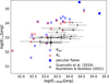 |
Fig. 15 X-ray flare energies from exponential fits normalized to Rqui (blue diamonds) and R0 (red circles), respectively, versus TESS flare energies for the 17 X-ray flares selected by eye. Energies of flares reported by Guarcello et al. (2019) and Kuznetsov & Kolotkov (2021) are marked in black. The peculiar flares described in Sect. 7.5.4 are marked by blue crosses. |
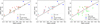 |
Fig. 16 X-ray flare energies from exponential fits normalized to R0 versus TESS flare energies. The energies calculated from fits made to the synthethic flare peaks (red) and normalized to R0 are compared with those made to the synthetic flare peak scaled down by a factor two (left panel, green circles) and up by factor two (middle panel, teal circles) respectively, and from fits made to the original synthetic peak but integrated over the flare light curve starting from the first eRASS bin (right panel, light green diamonds). The peculiar flares described in Sect. 7.5.4 are marked as blue crosses. The black line denotes equal optical and X-ray flare energies. |
7.5.4 Peculiar flares
Two stars, TIC 150359500 and TIC 278731274, each exhibited episodes of remarkable flare activity in both their TESS and eRASS light curves, that could not be treated with the above method. In both cases, several TESS flares occurred close in time and coincided with long-lasting, very strong episodes of X-ray brightening. A close up of these events is shown in Fig. 17). The times corresponding to the peaks of the TESS flares detected with our algorithm are marked with dashed vertical lines.
Since the X-ray counterparts of the individual TESS flare peaks could not be easily distinguished, we considered the episode as a whole, and we determined for each of the TESS and the eRASS light curves the total energy emitted throughout the flaring intervals. For eROSITA, we measured the integrated light over all the XFDPs in the two eRASS light curves starting from the first vertical dashed line in Fig. 17 that represents the onset of the optical flaring activity. For the X-ray event of TIC 150359500 we applied a linear interpolation to the XFDPs, as an exponential decay does not constrain the light curve well. For the X-ray event of TIC 278731274, we could fit an exponential decay to the XFDPs. We then integrated under these curves normalized to Rqui, to find the ED and then the X-ray flare energy, as in Sect. 7.5.3. For the peculiar X-ray flare on TIC 278731274, Rqui is equivalent to R0 as the flare decays to the quiescent state. We calculated the total optical energy emitted corresponding to the events that appear by visual inspection to be associated with the X-ray brightening by integrating over the corresponding time interval, that comprises for each of the two cases three optical flares identified by our detection algorithm but includes also some brightness enhancement above the rotational cycle that was not identified as flares by our automatic flare detection code. Notably, the duration of the flaring episodes for each of these two events (see Table 3) is longer than the rotational cycles of the stars. In such cases the reconstruction of the shape of the flare LC is particularly sensitive to a proper subtraction of the spot signal.
The energies emitted globally in these extraordinary events are listed in Table 3, and they are shown in the Ex,f – Eopt,f plot of Figs. 15 and 16 as large cross symbols. They are of the order of 1035 erg in both wavebands, at the high end of all flares seen in our sample and clearly in the superflare regime even considering the substantial uncertainties in the value of the X-ray flare energy. The two stars that exhibited these complex long-duration superflares are also among those with the highest flare frequency in our sample.
Complex optical flare events observed with TESS have been the subject of a dedicated study by Howard & MacGregor (2022). These authors found that ‘peak-bump’ morphologies, similar to the ones observed by us on TIC 150359500 and TIC 278731274, are typical for complex flares (representing 17% of the cases). Yang et al. (2023) show that a one-dimensional hydrodynamic model of a coronal flare loop with two heating sources, one at the loop apex and another one near the foot-points, can explain such morphologies. According to their study, the broad emission bump following the well-known impulsive flare phase represents optical continuum emission produced by a coronal plasma condensation that develops as a result of the long-lasting footpoint heat sources.
Bruno et al. (2024) fit optical ‘complex’ flares with a superposition of events each based on the flare template from Tovar Mendoza et al. (2022) which is a variant of the Davenport template used by us for the flare validation (see Sect. 6.1). They find that about 30% of flares observed with TESS at 20 s cadence and 40 % observed with CHEOPS (cadence 3 s) on late-K and M stars require at least two templates to fit the flare profile. Since our two ‘peculiar’ flares are composed each of three detected flares and a ‘bump-structure’, these events are among the rare particularly complex ones for which Bruno et al. (2024) find an occurrence rate of ~5 % or less. The occurrence of two complex events out of 58 detected flares in our M-dwarf sample is remarkably similar to this estimate.
A small number of remarkable complex optical flares is present in the literature dating before the advent of photometric monitoring space missions. A prime example is a giant flare on the M dwarf CN Leo for which Fuhrmeister et al. (2008) presents an optical light curve based on data from the UVES exposuremeter. After a ~10-long spike a broader bump and subsequent slower decay (lasting ~ 10 min) is observed (see Fig. 1 of Fuhrmeister et al. 2008 and close-up in Fig. 1 of Schmitt et al. 2008). Since the simultaneous U-band light curve obtained with XMM-Newton’s Optical Monitor showed an even longer decay, Fuhrmeister et al. (2008) ascribes the emission observed with the UVES photometer to continuum radiation.
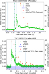 |
Fig. 17 Two long-duration flare episodes observed simultaneously with TESS (green) and in eRASS (blue diamonds) from the stars TIC 150359500 (top) and TIC 278731274 (bottom). The XFDPs (red) and the peaks of the TESS flares detected by the flare detection algorithm used in this paper (blue dashed lines) (see Sect. 6.1) are highlighted. |
Summed optical and X-ray flare energies Eopt,f and Ef,x, respectively, of multiple TESS and associated complex eRASS events.
8 Summary and conclusions
With TESS and eROSITA, for the first time in history, an optical and an X-ray (nearly) all-sky survey provide partial temporal overlap, giving access to simultaneous multi-wavelength time-series for statistical samples of active stars. In this work, we explore the capacities of joint TESS and eRASS light curves for our understanding of flares on M-dwarf stars. From a sample of ~300 M dwarfs with contemporaneous optical and X-ray light curve that are located in the ecliptic pole region, where both surveys have the highest temporal coverage, we selected the 25 most active ones.
Investigations of optical flares on late-type stars have obtained a boost during the last decade with the advent of space missions such as Kepler and TESS that – thanks to their high photometric data cadence – enable a detailed analysis of individual events. We detected 58 optical flares on the 25 M dwarfs of our sample. 23 of these events were in the superflare regime (Ef > 1033 erg) and one of them fulfilled the more stringent superflare definition of (Ef > 5 × 1034 erg) from Candelaresi et al. (2014), even though we considered only the energy emitted in the TESS band, that is, without correcting for bolometric emission. The most active among our stars likely have flare frequencies relevant for ozone depletion (Tilley et al. 2019) which is rather untypical for M dwarfs (Günther et al. 2022). We defer an investigation of this topic to a future work. The conservative estimate of the superflare rate in our sample is ~3.5 × 10⁻³ day−1, which is more than an order of magnitude higher than the estimate of Candelaresi et al. (2014). This high flare rate of our targets is likely to be attributed to the X-ray selection which favours active stars. Our bias is intentional as we do not aim at a representative sample but at a high probability to find bright enough events to be characterized in both wavebands.
Characterizing flares with eROSITA is more difficult, as during the survey mode, eROSITA makes a measurement of a given sky position only every 4 h, which is longer than the duration of many historical X-ray flares, such that it is impossible to extract the same amount of quantitative information as for the optical flares. Also, the starkly different data cadence makes it nontrivial to draw a relation between the brightenings seen in both wavebands.
To mitigate this we have defined a duty cycle of the fractional time the light curve deviates from the baseline ‘quiescent’ emission as a simple measure for the global variability in both X-ray and optical light curves. For the TESS observations of our sample we have shown that the duty cycle is well correlated with the traditional flare rate, that is the count of flare events per day. We thus suggest that the duty cycle can be used as a proxy for flare activity in case of poor data sampling. By comparing the optical and the X-ray duty cycle of our targets, we found a significant correlation, implying that stars that spend a higher fraction of time at enhanced X-ray emission levels also spend more time during optical flares. We found high duty cycles mostly among fast rotators (Prot ≲ 2 days), but a larger sample with a broader range of periods would be needed to establish a clear trend. The slowest rotator among the 25 M dwarfs had a period of 8.6 d, which may me due to a combination of our selection of particularly active stars and the TESS detection limit of ≲13 days.
To identify in a global way whether optical and X-ray flares are associated with each other, we searched each bin in the X-ray light curve, that is each eRODay, for TESS flares detected in its vicinity, which means up to 2 h before the eRODay. This ensures that no optical counterparts are missed, but implies that the X-ray flare – which presumably caused the enhanced X-ray bin – must have lasted for at least 1/2 eROday. This analysis allowed us to establish that X-ray light curves with a higher number of data points above the ‘quiescent’ emission level tend to have more optical flares preceding these apparent X-ray events (by ≲2 h).
To go beyond this coarse estimate of the association of X-ray and optical variability we put constraints on the X-ray flare parameters with help of the canonical (solar) flare scenario. The peak of the X-ray flare is expected to fall in most cases into the nearly 4 h data gap between two bins in the eRASS light curve. We constructed for each optical flare the predicted X-ray flare peak both in terms of its timing (few minutes after the optical flare) and its amplitude (constrained by the correlation with optical flare energy). Then we fitted the X-ray light curve starting with this reconstructed flare peak using an exponential function, and we derived the X-ray flare energy from the area under the fit function. A reasonable fit was obtained for 17 events, about 1/3 of the detected TESS flares. Our analysis has roughly doubled the number of joint optical/X-ray flares observed on M dwarfs. We found larger X-ray to optical flare energy ratios than those presented by Guarcello et al. (2019) and Kuznetsov & Kolotkov (2021) from Kepler observations , which might indicate that our sample consists of peculiar types of flares with high X-ray output, given that our sample is biased towards highly active stars.
On the other hand, the TESS flares of our stars are well sampled and, consequently, their energies Eopt,f are reliable. To constrain their X-ray counterparts we had to make several severe assumptions and approximations that involve significant uncertainties, which translate into the values of Ef,x. Our results agree to roughly one order of magnitude with the literature data for all the sanity checks with which we have estimated the errors on Ef,x, which therefore, can be considered to show that the solar-like flare scenario is a plausible explanation for the joint TESS and eRASS variability observed in M dwarfs. The most conservative estimate of our X-ray flare energies is in line with, for example, a superflare on AB Dor observed with TESS and eROSITA: For an optical flare with an energy of 4 × 1036 erg the X-ray flare was estimated to an energy of at most ~1035 erg (Schmitt et al. 2021). This event on AB Dor was observed from a poorly sampled eROSITA light curve, just as ours, where – similar to our results where Ex,f /Eopt,f ≳ 1 – the optical flare carried more energy than plausible estimates for the X-ray flare.
Two peculiar flare episodes on the stars TIC150359500 and TIC278731274 with uncharacteristically high X-ray and optical energies and long durations were found (see Table 3). These events exhibit a ‘peak-bump’ morphology which is typical for complex flares (Yang et al. 2023). Our rate of ~3 % for complex flare events that cannot be described by a simple fast-rise/exponential-like decay template is consistent with other recent studies of high-cadence space-based optical monitorings of late-type active stars. This relatively poorly explored category of events and the physics behind this phenomenon deserve more attention. We leave a more detailed investigation of the two peculiar flares and their role in the context of M-dwarf activity to a future study.
To summarize, simultaneous eROSITA and TESS data provide an entirely new window into statistical samples of stellar flares and many possibilities to test the solar-stellar connection.
The high uncertainty on the evolution of the X-ray variability resulting from the low (4 h) cadence of the eROSITA scanning mode is the major difficulty in an assessment of the physical parameters of the X-ray flares.
Acknowledgements
W.M.J. is supported by the Bundesministerium für Wirtschaft und Energie through the Deutsches Zentrum für Luft- und Raumfahrt e.V. (DLR) under grant number FKZ 50 OR 2208. EM is supported by Deutsche Forschungsgemeinschaft under grant STE 1068/8-1. This work is based on data from eROSITA, the soft X-ray instrument aboard SRG, a joint Russian-German science mission supported by the Russian Space Agency (Roskosmos), in the interests of the Russian Academy of Sciences represented by its Space Research Institute (IKI), and the Deutsches Zentrum für Luft- und Raumfahrt (DLR). The SRG spacecraft was built by Lavochkin Association (NPOL) and its subcontractors, and is operated by NPOL with support from the Max Planck Institute for Extraterrestrial Physics (MPE). The development and construction of the eROSITA X-ray instrument was led by MPE, with contributions from the Dr. Karl Remeis Observatory Bamberg & ECAP (FAU Erlangen-Nuernberg), the University of Hamburg Observatory, the Leibniz Institute for Astrophysics Potsdam (AIP), and the Institute for Astronomy and Astrophysics of the University of Tübingen, with the support of DLR and the Max Planck Society. The Argelander Institute for Astronomy of the University of Bonn and the Ludwig Maximilians Universität Munich also participated in the science preparation for eROSITA. The eROSITA data shown here were processed using the eSASS/NRTA software system developed by the German eROSITA consortium. This paper includes data collected by the TESS mission. Funding for the TESS mission is provided by the NASA’s Science Mission Directorate.
Appendix A Stellar parameters from Gaia, 2MASS, and TESS
Content of the 31 columns in our catalogue of the 25 X-ray bright or variable stars in the TESS SCVZ which correspond to photometry, TESS detection information, and stellar parameters.
Appendix B Stellar parameters from eRASS
Content of the eight columns in our catalogue of the 25 X-ray bright or variable stars in the TESS SCVZ which correspond to eRASS data and X-ray stellar parameters.
Appendix C Exponential fits to X-ray flares following optical TESS flares
Exponential fits to the 17 eRASS flare light curves that could be reasonably fit with a decaying exponential curve (Sect. 7.5.2) are shown in C.1 along with the synthetic X-ray flare peak(s), quiescent level (purple band), peak of TESS flare (dashed blue line) and XFDPs (red) (see Fig.14). The exponential fits are made to three synthetic peaks; the original (filled green square), inferred from TESS flare energies (Sect. 7.5) and the peak up-scaled (filled yellow circle) and down-scaled (filled purple triangle) respectively by a factor two as sanity checks (paragraph 7.5.3). The open symbols indicate the flare peaks obtained from the exponential fits.
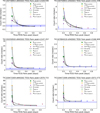 |
Fig. C.1 17 Exponential fits (black; see Sect. 7.5.2) to suspected X-ray flares in eRASS light curves following TESS flares. The Synthetic flare peaks (original, factor two upscaled and downscaled; see 7.5.1) and the flare peaks obtained from the corresponding fits are depicted by filled and open green squares, yellow circles and purple triangles respectively. |
References
- Astropy Collaboration (Robitaille, T. P., et al.) 2013, A&A, 558, A33 [NASA ADS] [CrossRef] [EDP Sciences] [Google Scholar]
- Astropy Collaboration (Price-Whelan, A. M., et al.) 2018, AJ, 156, 123 [Google Scholar]
- Astropy Collaboration (Price-Whelan, A. M., et al.) 2022, ApJ, 935, 167 [NASA ADS] [CrossRef] [Google Scholar]
- Benz, A. O. 2017, Living Rev. Solar Phys., 14, 2 [NASA ADS] [CrossRef] [Google Scholar]
- Brunner, H., Liu, T., Lamer, G., et al. 2022, A&A, 661, A1 [NASA ADS] [CrossRef] [EDP Sciences] [Google Scholar]
- Bruno, G., Pagano, I., Scandariato, G., et al. 2024, A&A, 686, A239 [NASA ADS] [CrossRef] [EDP Sciences] [Google Scholar]
- Candelaresi, S., Hillier, A., Maehara, H., Brandenburg, A., & Shibata, K. 2014, ApJ, 792, 67 [NASA ADS] [CrossRef] [Google Scholar]
- Cargill, P. J., & Priest, E. R. 1983, ApJ, 266, 383 [NASA ADS] [CrossRef] [Google Scholar]
- Castellanos Durán, J. S., & Kleint, L. 2020, ApJ, 904, 96 [CrossRef] [Google Scholar]
- Chabrier, G. 2001, ApJ, 554, 1274 [NASA ADS] [CrossRef] [Google Scholar]
- Davenport, J. R. A., Hawley, S. L., Hebb, L., et al. 2014, ApJ, 797, 122 [Google Scholar]
- Flaccomio, E., Micela, G., Sciortino, S., et al. 2018, A&A, 620, A55 [NASA ADS] [CrossRef] [EDP Sciences] [Google Scholar]
- Freedman, D., & Diaconis, P. 1981, Zeitsch. Wahrsch. Verwandte Gebiete, 57, 453 [CrossRef] [Google Scholar]
- Fuhrmeister, B., Liefke, C., Schmitt, J. H. M. M., & Reiners, A. 2008, A&A, 487, 293 [NASA ADS] [CrossRef] [EDP Sciences] [Google Scholar]
- Fuhrmeister, B., Lalitha, S., Poppenhaeger, K., et al. 2011, A&A, 534, A133 [NASA ADS] [CrossRef] [EDP Sciences] [Google Scholar]
- Gaia Collaboration (Prusti, T., et al.) 2016, A&A, 595, A1 [NASA ADS] [CrossRef] [EDP Sciences] [Google Scholar]
- Gaia Collaboration (Brown, A. G. A., et al.) 2018, A&A, 616, A1 [NASA ADS] [CrossRef] [EDP Sciences] [Google Scholar]
- Guarcello, M. G., Micela, G., Sciortino, S., et al. 2019, A&A, 622, A210 [NASA ADS] [CrossRef] [EDP Sciences] [Google Scholar]
- Güdel, M., Schmitt, J. H. M. M., Bookbinder, J. A., & Fleming, T. A. 1993, ApJ, 415, 236 [CrossRef] [Google Scholar]
- Günther, M. N., Zhan, Z., Seager, S., et al. 2020, AJ, 159, 60 [Google Scholar]
- Günther, M. N., Berardo, D. A., Ducrot, E., et al. 2022, AJ, 163, 144 [CrossRef] [Google Scholar]
- Harris, C. R., Millman, K. J., van der Walt, S. J., et al. 2020, Nature, 585, 357 [NASA ADS] [CrossRef] [Google Scholar]
- Hawley, S. L., Davenport, J. R. A., Kowalski, A. F., et al. 2014, ApJ, 797, 121 [Google Scholar]
- Howard, W. S., & MacGregor, M. A. 2022, ApJ, 926, 204 [NASA ADS] [CrossRef] [Google Scholar]
- Howard, A. W., Marcy, G. W., Bryson, S. T., et al. 2012, ApJS, 201, 15 [Google Scholar]
- Hudson, H. S. 1991, Sol. Phys., 133, 357 [Google Scholar]
- Hudson, H. S. 2011, Space Sci. Rev., 158, 5 [NASA ADS] [CrossRef] [Google Scholar]
- Hunt-Walker, N. M., Hilton, E. J., Kowalski, A. F., Hawley, S. L., & Matthews, J. M. 2012, PASP, 124, 545 [NASA ADS] [CrossRef] [Google Scholar]
- Jao, W.-C., Henry, T. J., Gies, D. R., & Hambly, N. C. 2018, ApJ, 861, L11 [NASA ADS] [CrossRef] [Google Scholar]
- Joy, A. H., & Humason, M. L. 1949, PASP, 61, 133 [CrossRef] [Google Scholar]
- Kaltenegger, L., Pepper, J., Stassun, K., & Oelkers, R. 2019, ApJ, 874, L8 [NASA ADS] [CrossRef] [Google Scholar]
- Katsova, M. M., Livshits, M. A., & Schmitt, J. H. M. M. 2002, Stellar Coronae in the Chandra and XMM-NEWTON Era, eds. F. Favata, & J. J. Drake, ASP Conf. Ser., 277, 515 [NASA ADS] [Google Scholar]
- Kawai, H., Tsuboi, Y., Iwakiri, W. B., et al. 2022, PASJ, 74, 477 [NASA ADS] [CrossRef] [Google Scholar]
- Kretzschmar, M. 2011, A&A, 530, A84 [NASA ADS] [CrossRef] [EDP Sciences] [Google Scholar]
- Kuznetsov, A. A., & Kolotkov, D. Y. 2021, ApJ, 912, 81 [NASA ADS] [CrossRef] [Google Scholar]
- Lomb, N. R. 1976, Ap&SS, 39, 447 [Google Scholar]
- Magaudda, E., Stelzer, B., Covey, K. R., et al. 2020, A&A, 638, A20 [NASA ADS] [CrossRef] [EDP Sciences] [Google Scholar]
- Magaudda, E., Stelzer, B., & Raetz, S. 2022a, Astron. Nachr., 343, e20220049 [NASA ADS] [CrossRef] [Google Scholar]
- Magaudda, E., Stelzer, B., Raetz, S., et al. 2022b, A&A, 661, A29 [NASA ADS] [CrossRef] [EDP Sciences] [Google Scholar]
- Mann, A. W., Feiden, G. A., Gaidos, E., Boyajian, T., & von Braun, K. 2015, ApJ, 804, 64 [Google Scholar]
- McQuillan, A., Aigrain, S., & Mazeh, T. 2013, MNRAS, 432, 1203 [Google Scholar]
- Merloni, A., Larmer, G., Liu, T., et al. 2024, A&A, 682, A34 [NASA ADS] [CrossRef] [EDP Sciences] [Google Scholar]
- Namekata, K., Sakaue, T., Watanabe, K., et al. 2017, ApJ, 851, 91 [Google Scholar]
- Namekata, K., Maehara, H., Sasaki, R., et al. 2020, PASJ, 72 [Google Scholar]
- Predehl, P., Andritschke, R., Arefiev, V., et al. 2021, A&A, 647, A1 [EDP Sciences] [Google Scholar]
- Raetz, S., Stelzer, B., Damasso, M., & Scholz, A. 2020, A&A, 637, A22 [NASA ADS] [CrossRef] [EDP Sciences] [Google Scholar]
- Reiners, A., Schüssler, M., & Passegger, V. M. 2014, ApJ, 794, 144 [Google Scholar]
- Ricker, G. R., Winn, J. N., Vanderspek, R., et al. 2014, SPIE Conf. Ser., 9143, 914320 [Google Scholar]
- Riello, M., De Angeli, F., Evans, D. W., et al. 2018, A&A, 616, A3 [NASA ADS] [CrossRef] [EDP Sciences] [Google Scholar]
- Robrade, J., & Schmitt, J. H. M. M. 2005, A&A, 435, 1073 [NASA ADS] [CrossRef] [EDP Sciences] [Google Scholar]
- Scargle, J. D. 1982, ApJ, 263, 835 [Google Scholar]
- Schmitt, J. H. M. M., Reale, F., Liefke, C., et al. 2008, A&A, 481, 799 [NASA ADS] [CrossRef] [EDP Sciences] [Google Scholar]
- Schmitt, J. H. M. M., Ioannidis, P., Robrade, J., et al. 2021, A&A, 652, A135 [NASA ADS] [CrossRef] [EDP Sciences] [Google Scholar]
- Scott, D. W. 2009, WIREs Computat. Stat., 1, 303 [CrossRef] [Google Scholar]
- Shibayama, T., Maehara, H., Notsu, S., et al. 2013, ApJS, 209, 5 [Google Scholar]
- Stassun, K. G. 2019, VizieR Online Data Catalog: IV/38 [Google Scholar]
- Stelzer, B., Schmitt, J. H. M. M., Micela, G., & Liefke, C. 2006, A&A, 460, L35 [NASA ADS] [CrossRef] [EDP Sciences] [Google Scholar]
- Stelzer, B., Damasso, M., Scholz, A., & Matt, S. P. 2016, MNRAS, 463, 1844 [NASA ADS] [CrossRef] [Google Scholar]
- Stassun, K. G., Oelkers, R. J., Pepper, J., et al. 2018, AJ, 156, 102 [Google Scholar]
- Stelzer, B., Bogner, M., Magaudda, E., & Raetz, S. 2022a, A&A, 665, A30 [NASA ADS] [CrossRef] [EDP Sciences] [Google Scholar]
- Stelzer, B., Caramazza, M., Raetz, S., Argiroffi, C., & Coffaro, M. 2022b, A&A, 667, A9 [NASA ADS] [CrossRef] [EDP Sciences] [Google Scholar]
- Sunyaev, R., Arefiev, V., Babyshkin, V., et al. 2021, A&A, 656, A132 [NASA ADS] [CrossRef] [EDP Sciences] [Google Scholar]
- Tarter, J. C., Backus, P. R., Mancinelli, R. L., et al. 2007, Astrobiology, 7, 30 [NASA ADS] [CrossRef] [Google Scholar]
- Tilley, M. A., Segura, A., Meadows, V., Hawley, S., & Davenport, J. 2019, Astrobiology, 19, 64 [Google Scholar]
- Tovar Mendoza, G., Davenport, J. R. A., Agol, E., Jackman, J. A. G., & Hawley, S. L. 2022, AJ, 164, 17 [CrossRef] [Google Scholar]
- Truemper, J. 1982, Adv. Space Res., 2, 241 [Google Scholar]
- VanderPlas, J. T. 2018, ApJS, 236, 16 [Google Scholar]
- Vanderspek, R., Doty, J. P., Fausnaugh, M., et al. 2018, TESS Instrument Handbook, https://archive.stsci.edu/missions/tess/doc/TESS_Instrument_Handbook_v8.1.pdf [Google Scholar]
- Veronig, A., Temmer, M., Hanslmeier, A., Otruba, W., & Messerotti, M. 2002, A&A, 382, 1070 [NASA ADS] [CrossRef] [EDP Sciences] [Google Scholar]
- Wright, N. J., Drake, J. J., Mamajek, E. E., & Henry, G. W. 2011, ApJ, 743, 48 [Google Scholar]
- Yang, K. E., Sun, X., Kerr, G. S., & Hudson, H. S. 2023, ApJ, 959, 54 [NASA ADS] [CrossRef] [Google Scholar]
Archive available at https://gea.esac.esa.int/archive/
BP and RP represent the integrated fluxes from the Gaia BP and RP spectrophotometers, which were available with Gaia DR2 data (Riello et al. 2018)
All Tables
TIC ID, quiescent rate from eRASS 2 (Rqui,eRASS2), eRASS 3 (Rqui,eRASS3), the mean quiescent rate (Rqui,mean), and the standard deviation (Rqui,std,dev) from the two surveys in cts s−1, eRASS duty cycle of eRASS 2 (vx,DC,eRASS2), eRASS 3 (vx,DC,eRASS3), the mean eRASS duty cycle (vx,DC,mean), and the standard deviation (vx,DC,std,dev) of the two eRASS surveys.
Rotation periods and optical variability diagnostics derived from TESS light curves.
Summed optical and X-ray flare energies Eopt,f and Ef,x, respectively, of multiple TESS and associated complex eRASS events.
Content of the 31 columns in our catalogue of the 25 X-ray bright or variable stars in the TESS SCVZ which correspond to photometry, TESS detection information, and stellar parameters.
Content of the eight columns in our catalogue of the 25 X-ray bright or variable stars in the TESS SCVZ which correspond to eRASS data and X-ray stellar parameters.
All Figures
|
Fig. 1 Colour-magnitude diagram for M dwarfs in the TESS SCVZ (cyan) with the two samples defined in Sect. 3.4 highlighted in green (count rate ≥ 1 cts s−1) and red (count rate ratio between eRASS2 and eRASS3 ≥ 2 cts s−1). The overlap between the two samples are marked in orange. Overplotted is the main sequence isochrone (black) from the table ‘A Modern Mean Dwarf Stellar Color and Effective Temperature Sequence’ by E. Mamajek (https://www.pas.rochester.edu/~emamajek/EEM_dwarf_UBVIJHK_colors_Teff.txt). |
| In the text | |
|
Fig. 2 Distribution of distances for the two subsamples that are X-ray brightest and the most X-ray variable defined in Sect. 3.4 as well as the entire M-dwarf sample in the TESS SCVZ described in Sect. 3.2. |
| In the text | |
|
Fig. 3 Variation of the X-ray count rate in the 0.2–5.0 ke V band between eRASS2 and eRASS3 for the M dwarfs in the TESS SCVZ. Left panel – all stars, right panel – zoom into the low count rate region. The lines denote equal count rates in both surveys (solid) and differences of a factor two (dashed). The X-ray brightest stars (Eq. (1)) are high-lighted in red, the most X-ray variable (Eq. (2)) in green and stars that fulfil both critera in lime. See Sect. 3.4 for details. |
| In the text | |
|
Fig. 4 Distribution of rotation periods of our final M-dwarf sample of the X-ray brightest or most X-ray variable stars (blue) and of the sample of all M dwarfs detected in a 10-month observational period of the 4-year Kepler mission from McQuillan et al. (2013) (green). |
| In the text | |
|
Fig. 5 Example of an eRASS light curve (the M dwarf TIC278731274 observed in eRASS2) demonstrating the definition of the quiescent count rate level, Rqui, and the selection of variable light curve bins (namely eROdays significantly above Rqui; see text in Sects. 5.2 and 5.3) |
| In the text | |
|
Fig. 6 Relation between X-ray activity and rotation of our sample (large triangles and squares are for eRASS2 and eRASS3, respectively) compared to the M-dwarf samples from Magaudda et al. (2020, 2022b) (dots). The stars are colour-coded by mass and lines connect the two epochs for a given star from our sample. |
| In the text | |
|
Fig. 7 Optical flare frequency distributions of the 22 targets with flares detected in the TESS light curves of the sectors overlapping with eRASS (circles). For comparison the FFDs for the fast rotating M dwarfs from the catalog by Kaltenegger et al. (2019) that were studied by Stelzer et al. (2022a) are shown ( small crosses). |
| In the text | |
|
Fig. 8 TESS duty cycle νo,DC versus TESS flare rate νo,f, along with a linear fit to the data (blue line). For each star, the TESS results from the data overlapping in time with the eRASS2 and eRASS3 light curve, respectively, are distinguished by different colours. |
| In the text | |
|
Fig. 9 TESS mean duty cycle versus eRASS mean duty cycle, with the standard deviations between the values from the two eRASS epochs represented as uncertainties. |
| In the text | |
|
Fig. 10 X-ray duty cycle vx,DC,mean versus rotation period (left) and optical duty cycle vo,DC,mean versus rotation period (right). Lines connect the two epochs for a given star. |
| In the text | |
|
Fig. 11 Example of an eRASS light curved binned at 40 s, with bins close in time being combined (orange) and the same light curve binned at 1 eRODay. For this example the time-shift between the two light curves is roughly 2 h or 1/2 eRODay. |
| In the text | |
|
Fig. 12 Example of a flattened TESS light curve and eRASS light curve for TIC 220473309 observed during the eRASS2 epoch of the star. The eRASS data points significantly above the quiescent level (purple-shaded area), also named as the ‘X-ray flare data points’ (XFDPs), are marked in red. The TESS flare data points are marked in dark blue. XFDPs around which TESS flares were found are marked as green squares, and the vertical bins of width 1 eROday in which they lie are marked with dashed blue lines. |
| In the text | |
|
Fig. 13 XFDPs that are preceded by TESS flares versus all XFDPs per eRASS light curve. The orange, blue and green lines denote 20%, 10% and 5% of XFDPs that are preceded by TESS flares, respectively. |
| In the text | |
|
Fig. 14 eRASS3 light curve of TIC 220473309 illustrating our estimate of the X-ray flare peak (green data point) as explained in Sect. 7.5.1 and the exponential fit to the flare decay (black curve) described in Sect. 7.5.2. |
| In the text | |
|
Fig. 15 X-ray flare energies from exponential fits normalized to Rqui (blue diamonds) and R0 (red circles), respectively, versus TESS flare energies for the 17 X-ray flares selected by eye. Energies of flares reported by Guarcello et al. (2019) and Kuznetsov & Kolotkov (2021) are marked in black. The peculiar flares described in Sect. 7.5.4 are marked by blue crosses. |
| In the text | |
|
Fig. 16 X-ray flare energies from exponential fits normalized to R0 versus TESS flare energies. The energies calculated from fits made to the synthethic flare peaks (red) and normalized to R0 are compared with those made to the synthetic flare peak scaled down by a factor two (left panel, green circles) and up by factor two (middle panel, teal circles) respectively, and from fits made to the original synthetic peak but integrated over the flare light curve starting from the first eRASS bin (right panel, light green diamonds). The peculiar flares described in Sect. 7.5.4 are marked as blue crosses. The black line denotes equal optical and X-ray flare energies. |
| In the text | |
|
Fig. 17 Two long-duration flare episodes observed simultaneously with TESS (green) and in eRASS (blue diamonds) from the stars TIC 150359500 (top) and TIC 278731274 (bottom). The XFDPs (red) and the peaks of the TESS flares detected by the flare detection algorithm used in this paper (blue dashed lines) (see Sect. 6.1) are highlighted. |
| In the text | |
|
Fig. C.1 17 Exponential fits (black; see Sect. 7.5.2) to suspected X-ray flares in eRASS light curves following TESS flares. The Synthetic flare peaks (original, factor two upscaled and downscaled; see 7.5.1) and the flare peaks obtained from the corresponding fits are depicted by filled and open green squares, yellow circles and purple triangles respectively. |
| In the text | |
Current usage metrics show cumulative count of Article Views (full-text article views including HTML views, PDF and ePub downloads, according to the available data) and Abstracts Views on Vision4Press platform.
Data correspond to usage on the plateform after 2015. The current usage metrics is available 48-96 hours after online publication and is updated daily on week days.
Initial download of the metrics may take a while.