| Issue |
A&A
Volume 698, May 2025
|
|
|---|---|---|
| Article Number | A115 | |
| Number of page(s) | 16 | |
| Section | Planets, planetary systems, and small bodies | |
| DOI | https://doi.org/10.1051/0004-6361/202554172 | |
| Published online | 06 June 2025 | |
Radial variations in the nitrogen, carbon, and hydrogen fractionation in the PDS 70 planet-hosting disk
1
Dipartimento di Fisica, Università degli Studi di Milano,
Via Celoria 16,
20133
Milano,
Italy
2
Departamento de Astronomía, Universidad de Chile,
Camino El Observatorio 1515, Las Condes,
Santiago,
Chile
3
Max-Planck Institute for Astronomy (MPIA),
Königstuhl 17,
69117
Heidelberg,
Germany
4
Center for Astrophysics | Harvard & Smithsonian,
60 Garden St.,
Cambridge,
MA
02138,
USA
5
Department of Earth, Atmospheric, and Planetary Sciences, Massachusetts Institute of Technology,
Cambridge,
MA
02139,
USA
6
Department of Astronomy, University of Florida,
Gainesville,
FL
32611,
USA
7
Department of Astronomy, University of Virginia,
Charlottesville,
VA
22904,
USA
8
Center for Exoplanets and Habitable Worlds, Penn State University,
525 Davey Laboratory, 251 Pollock Road,
University Park,
PA
16802,
USA
9
Department of Astronomy & Astrophysics, The Pennsylvania State University,
525 Davey Laboratory,
University Park,
PA
16802,
USA
★ Corresponding author: luna.rampinelli@unimi.it
Received:
18
February
2025
Accepted:
1
April
2025
Element isotopic ratios are powerful tools for reconstructing the journey of planetary material from the parental molecular cloud to protoplanetary disks, where planets form and accrete their atmosphere. Radial variations in the isotopic ratios in protoplanetary disks reveal local pathways that can critically affect the degree of isotope fractionation of planetary material. We present spatially resolved profiles of the 14N/15N, 12C/13C, and D/H isotopic ratios of the HCN molecule in the PDS 70 disk, which hosts two actively accreting giant planets. ALMA observations of HCN, H13CN, HC15N, and DCN with a high spatial resolution reveal radial variations in the fractionation profiles. We extracted the HCN/HC15N ratio out to ~120 au. It shows a decreasing trend outside the inner cavity wall of the PDS 70 disk, which is located at ~50 au. We suggest that the radial variations observed in the HCN/HC15N ratio are linked to isotope-selective photodissociation of N2. We leveraged the spectrally resolved hyperfine component of the HCN line to extract the radial profile of the HCN/H13CN ratio between ~40 and 90 au and obtained a value that is consistent with the 12C/13C ratio in the interstellar medium. The deuteration profile is also mostly constant throughout the disk, with a DCN/HCN ratio ~0.02 that is in line with other disk-averaged values and radial profiles in disks around T Tauri stars. The extracted radial profiles of isotopolog ratios show that different fractionation processes dominate at different spatial scales in the planet-hosting disk of PDS 70.
Key words: astrochemistry / protoplanetary disks / stars: individual: PDS 70
© The Authors 2025
 Open Access article, published by EDP Sciences, under the terms of the Creative Commons Attribution License (https://creativecommons.org/licenses/by/4.0), which permits unrestricted use, distribution, and reproduction in any medium, provided the original work is properly cited.
This article is published in open access under the Subscribe to Open model. Subscribe to A&A to support open access publication.
1 Introduction
The process of planet formation is expected to leave imprints on the natal environment, that is, on the protoplanetary disk, such as dust substructures (see, e.g., Andrews et al. 2018; Sierra et al. 2021; Benisty et al. 2023), kinematic deviations in the rotation pattern of the gas (see, e.g., Perez et al. 2015; Pinte et al. 2023; Izquierdo et al. 2023), or chemical signatures (see, e.g., Cleeves et al. 2015; Law et al. 2023; Booth et al. 2023). The capabilities of both ground-based facilities and space missions have enabled a large variety of indirect evidence of ongoing planet formation in protoplanetary disks to be detected, including the first multiwavelength direct detection of two accreting gas giants in the transition disk around PDS 70 (Keppler et al. 2018; Haffert et al. 2019; Benisty et al. 2021; Zhou et al. 2021).
The first chemical inventory of the PDS 70 disk (Facchini et al. 2021) and recent high-resolution line emission observations (Rampinelli et al. 2024) showed a complex structured emission morphology of molecular tracers that highlights the strong link between forming planets and their natal environment. In particular, most of the molecules show a ring-shaped emission that is colocated with the cavity wall and the peak in the scattered light from micrometer dust (Keppler et al. 2018). This is consistent with the presence of a deep gas gap in the PDS 70 disk (Keppler et al. 2019; Portilla-Revelo et al. 2023; Law et al. 2024) and feeds back into the chemical makeup of the planets that are forming (see, e.g., Cridland et al. 2023; Leemker et al. 2024; Hsu et al. 2024).
Multiple aspects of disk chemistry are linked to the process of planet formation (see, e.g., Öberg & Bergin 2021; Öberg et al. 2023, and references therein), such as the location of snow-lines (Öberg et al. 2011; Okuzumi & Tazaki 2019), the ratios of the main elements H, C, O, and N (Cridland et al. 2020; Drazkowska et al. 2023; Jiang et al. 2023), or isotopic ratios (Altwegg et al. 2019; Nomura et al. 2023). The latter can be an efficient tool for tracing the origin of planetary material back because it stores important markings of the history of gas and solids from the molecular cloud, down to rocky cores and planetary atmospheres that build in protoplanetary disks (Nomura et al. 2023). The isotopic levels in solids and gas have been used to reconstruct the origin of volatiles in Solar System objects (Morbidelli et al. 2000; Aléon 2010; Marty 2012; Ceccarelli et al. 2014; Albertsson et al. 2014; Altwegg et al. 2019). The isotopic ratios of molecules are primarily set when molecules form, but various environmental conditions during the timeline of planet formation can reset or alter these values. This is highlighted by the wide range of isotopic ratios in different Solar System bodies, in particular, for D/H and 14N/15N (see, e.g., Nomura et al. 2023, and references therein). The first measurement of the 14NH3/15NH3 ratio for a brown dwarf atmosphere was presented by Barrado et al. (2023), who reported a value of ~670, which is consistent with star-like formation by gravitational collapse. This result also carved the path toward direct isotopolog ratios measurements in exoplanetary atmospheres. In particular, a measurement of 12CO/13CO has been presented for the first time for exoplanetary atmospheres (Zhang et al. 2021; Gandhi et al. 2023) and showed 12C/13C values that were lower than those in the interstellar medium (ISM).
These recent breakthroughs show the potential of isotopic imprints to trace the origins of the Solar System and of exoplanets. In this context, direct constraints on the isotopic ratios in the stage of protoplanetary disks are fundamental, in which planets build their cores and accrete their atmospheres. Disk-integrated isotopolog ratios have been achieved in a variety of molecular tracers, including CO, HCN, CN, C2H, and HCO+ (Smith et al. 2009; Öberg et al. 2012; Guzmán et al. 2015, 2017; Zhang et al. 2017; Huang et al. 2017; Hily-Blant et al. 2017, 2019; Yoshida et al. 2022, 2024; Bergin et al. 2024). These results provided first insights into the main chemical processes that drive the fractionation in disks: For example, both warm and cold gas-phase deuteration pathways were suggested to take place in disks, while isotope-selective photodissociation was proposed to play a crucial role for the nitrogen fractionation (see Nomura et al. 2023 for a recent review). Moreover, a first comparison with earlier and later stages of star and planet formation revealed the importance of comparing isotopolog ratios extracted from the same molecule because fractionation processes can lead to very different isotope ratios in different tracers (Bergin et al. 2024). Finally, these diskintegrated results already varied strongly from the ISM isotopic ratios.
On the other hand, disk-integrated ratios do not fully capture the chemical complexity of protoplanetary disks. This is expected to induce spatial variations in the isotopic ratios as different fractionation processes dominate at different scales and in different disk regions. Radially resolved isotopolog ratios were extracted in the MAPS (Molecules with ALMA at Planet-forming Scales) sample for DCN/HCN (Cataldi et al. 2021), for HCN/HC15N in the TW Hya (Hily-Blant et al. 2019) the V4046 Sgr disks (Nomura et al. 2023, Guzmán et al., in prep.), and for 13CO/C18O in the TW Hya disk (Furuya et al. 2022).
We present the radial profile of the nitrogen, carbon, and hydrogen fractionation of the HCN molecule in the PDS 70 disk, in which two protoplanets are accreting their atmospheres. In Section 2 we present the ALMA line emission observations we analyzed. In Section 3 we reconstruct the radial profiles of the column density of the HCN isotopologs and the related isotopolog ratios. We discuss the results in Section 4 and summarize our conclusions in Section 5.
2 Observations
We used ALMA band 6 and 7 line emission observations from projects 2019.1.01619.S (PI S. Facchini) and 2022.1.01695.S (PI M. Benisty). The observations include various lines of HCN isotopologs: HCN (4–3), H13CN (3–2), H13CN (4–3), HC15N (3–2), HC15N (4–3), and DCN (3–2).
The band 7 observations consist of four execution blocks (EBs): one short-baseline (SB; ALMA configuration C-4; the maximum baseline is 0.8 km) and three long-baseline configurations (LB; configuration C-7; the maximum baseline is 3.6 km). The spectral setup includes four spectral windows (spws) that were initially intended for continuum observations, each with a bandwidth of 1.875 GHz, 1920 channels, and a resolution of 977 kHz. The spws cover the same frequency ranges in all EBs: 342.483–344.358 GHz for spw 0, 344.379–346.254 GHz for spw 1, 354.483–356.358 GHz for spw 2, and 356.441–358.316 GHz for spw 3. Each EB had 35 minutes of on-source time for a total of 2.33 hours. All the EBs were initially calibrated using the ALMA pipeline, which was followed by self-calibration based on the pipeline designed by the exoALMA Large Program (Loomis et al. 2025) using the software CASA (CASA Team 2022), version 6.2. We first flagged the lines in our frequency range (see Table A.1): CS (7–6, ν = 342.88 GHz), HC15N (4–3, ν = 344.20 GHz), H13CN (4–3, ν = 345.34 GHz, 12CO (3–2, ν = 345.80 GHz), HCN (4–3, ν = 354.51 GHz), HCO+ (4–3, ν = 356.73 GHz), and SO (88−77, ν = 344.31 GHz). We flagged the range between −30 km/s to +30 km/s around each line center. The remaining unflagged data were averaged into 250 MHz wide channels. A first round of phase-only self-calibration was performed on each EB separately, for which we combined the scans and spws on time intervals over the full EB duration. The EBs were then aligned by regridding them to a common uv-grid with natural weighting, and we only retained overlapping grid cells and applied phase shifts to minimize the visibility differences (Loomis et al. 2025). No flux rescaling was necessary because the flux offsets between EBs were very small (<1%). Next, phase-only self-calibration was applied to the SB EB using models created with the task tclean, cleaning down to 6σ at each round. Multiple rounds with progressively shorter solution intervals were used (EB-long, 360 s, 120 s, 60 s, and 20 s), and we stopped when the signal-to-noise ratio (S/N) and noise structure began to degrade. The self-calibrated SB EB was then concatenated with the three LB EBs, and the phase-only self-calibration was repeated on the combined dataset. Similar to before, we cleaned down to 6σ at each step, with progressively shorter solution intervals (EB-long, 360 s, 120 s, 60 s, 30 s, and 18 s). After this, the data were cleaned down to 1σ, and two rounds of amplitude and phase self-calibration were performed, for which we combined polarizations and spws. The first round used EB-long intervals, and the second round used scan-long intervals. Gain solutions and phase shifts were then applied to the full spectral data, including the line emission channels, following exactly the same order. To reduce the size of the dataset, the full spectral data were binned into 30s intervals. Finally, continuum subtraction was performed on all datasets using the uvcontsub task. The self-calibration of band 6 data was performed as described in Law et al. (2024); Rampinelli et al. (2024).
We imaged the lines using the tclean task (Högbom 1974; Cornwell 2008) implemented in the CASA software (CASA Team 2022) v6.65. In particular, we used a multiscale deconvolver with scales [0,5,10,20,30] pixels, where the pixel size is ~![$\[0^{\prime\prime}_\cdot02\]$](/articles/aa/full_html/2025/06/aa54172-25/aa54172-25-eq1.png) , and a flux threshold of 3.5σ. We performed a first CLEANing without applying any mask, and a second CLEANing iteration using a mask built by selecting the signal >7σ in the previous iteration (Loomis et al. 2025). We applied the so-called JvM correction (Jorsater & van Moorsel 1995) following Czekala et al. (2021) by rescaling the residual map by the ratio of the areas of the CLEAN and DIRTY beams (ϵ) to correct for the unit mismatch between the model and residual image (see Table B.1 for the ϵ values corresponding to each cube). More details of the CLEANing strategies can be found in Rampinelli et al. (2024). The following analysis was performed on continuum-subtracted cubes and JvM corrected cubes, except for the uncertainty evaluation, which might be underestimated by the JvM correction (Casassus & Cárcamo 2022) because the residuals are rescaled. In the following analysis, we also assumed the geometrical parameters M* = 0.875 M⊙, i = 51.7°, PA = 160.4°, and vsys = 5.5 km s−1 (in LSRK frame), as they were obtained by Keppler et al. (2019), and a distance of 113 pc (Gaia Collaboration 2018).
, and a flux threshold of 3.5σ. We performed a first CLEANing without applying any mask, and a second CLEANing iteration using a mask built by selecting the signal >7σ in the previous iteration (Loomis et al. 2025). We applied the so-called JvM correction (Jorsater & van Moorsel 1995) following Czekala et al. (2021) by rescaling the residual map by the ratio of the areas of the CLEAN and DIRTY beams (ϵ) to correct for the unit mismatch between the model and residual image (see Table B.1 for the ϵ values corresponding to each cube). More details of the CLEANing strategies can be found in Rampinelli et al. (2024). The following analysis was performed on continuum-subtracted cubes and JvM corrected cubes, except for the uncertainty evaluation, which might be underestimated by the JvM correction (Casassus & Cárcamo 2022) because the residuals are rescaled. In the following analysis, we also assumed the geometrical parameters M* = 0.875 M⊙, i = 51.7°, PA = 160.4°, and vsys = 5.5 km s−1 (in LSRK frame), as they were obtained by Keppler et al. (2019), and a distance of 113 pc (Gaia Collaboration 2018).
We first imaged all lines with natural weighting. Table 1 lists the image properties, including the channel width, beam size, and RMS, and the properties of the molecular transitions. The RMS was evaluated as the standard deviation in the first and last five channels of each cube. A list of detected lines with the corresponding line fluxes is listed in Table A.1, which also includes band 6 lines that were previously presented by Rampinelli et al. (2024) for comparison. The line fluxes where obtained as described in Appendix A (band 7) and Rampinelli et al. (2024) (band 6).
In order to perform the analysis outlined in Sect. 3, we imaged all the cubes with two different sets of parameters to maximize the sensitivity of the band 6 and 7 observations. Each time uv-taper and/or robust were chosen to obtain cubes with the same spatial resolution. In particular, cubes imaged to maximize the band 6 and 7 sensitivity correspond to beam major axes of ~![$\[0^{\prime\prime}_\cdot20\]$](/articles/aa/full_html/2025/06/aa54172-25/aa54172-25-eq8.png) (~23 au) and ~
(~23 au) and ~![$\[0^{\prime\prime}_\cdot14\]$](/articles/aa/full_html/2025/06/aa54172-25/aa54172-25-eq9.png) (~15 au), respectively. The corresponding weighting, uv-taper, beam size, beam area, and RMS for the two imaging rounds are listed in Table B.1.
(~15 au), respectively. The corresponding weighting, uv-taper, beam size, beam area, and RMS for the two imaging rounds are listed in Table B.1.
We calculated integrated-intensity maps of the imaged cubes using the bettermoments package (Teague & Foreman-Mackey 2019) by integrating data cubes over a velocity range in which each line showed emission in the channel maps. Figure 1 shows an example of the maps we obtained for each line (see the last column of Table 1). The map in the bottom right panel of Fig. 1 was obtained from SB observations only, which completely cover the HCN (4–3) line, while LB observations spectrally cover only half of the line. This allowed us to reconstruct half of the azimuthal extent of the disk. We analyzed the cube that covered half of the HCN (4–3) line, which we obtained from combined SB and LB observations, because a high angular resolution is needed to separate the hyperfine component (see Appendix B for more details).
Listed imaged lines, corresponding rest frequencies, line properties, and imaging parameters (channel width, beam, and RMS).
3 Results
3.1 Radial rotational diagram
From the integrated-intensity maps in Fig. 1, we extracted the radial profiles of the integrated intensity of each line using the GoFish package (Teague 2019). In order to limit the beam dilution when we performed the azimuthal average, we tried to extract the radial profiles of the integrated intensity only from a wedge of ±30° along the disk major axis. However, the resulting S/N for DCN and HC15N in particular was too low for the analysis we present here. We therefore extracted the integrated-intensity profiles by performing a complete azimuthal average over annuli with a width of ![$\[0^{\prime\prime}_\cdot1\]$](/articles/aa/full_html/2025/06/aa54172-25/aa54172-25-eq10.png) . The resulting profiles are plotted in the top panels in Fig. 2. The dashed black line shows the integrated-intensity profile of the 855 μm continuum observations (Isella et al. 2019; Benisty et al. 2021, corresponding beam major axis of
. The resulting profiles are plotted in the top panels in Fig. 2. The dashed black line shows the integrated-intensity profile of the 855 μm continuum observations (Isella et al. 2019; Benisty et al. 2021, corresponding beam major axis of ![$\[0^{\prime\prime}_\cdot05\]$](/articles/aa/full_html/2025/06/aa54172-25/aa54172-25-eq11.png) ).
).
As two lines are detected for both HC15N and H13CN, with upper energies ranging from ~25 to 41 K, we were able to apply the rotational diagram (Goldsmith & Langer 1999) analysis to extract their molecular column density Nt and excitation temperature Tex as follows:
![$\[\ln~ \frac{N_{\mathrm{u}}}{g_{\mathrm{u}}}=~\ln~ N_{\mathrm{t}}-~\ln~ Q\left(T_{\mathrm{ex}}\right)-\frac{E_{\mathrm{u}}}{\mathrm{k}_{\mathrm{B}} T_{\mathrm{ex}}},\]$](/articles/aa/full_html/2025/06/aa54172-25/aa54172-25-eq12.png) (1)
(1)
where Nu, gu, and Eu are the upper-state column density, degeneracy, and energy, respectively; Nt is the total molecular column density; kB is the Boltzman constant; Tex is the excitation temperature; and Q(Tex) is the partition function. In the optically thin assumption, Nu depends on the integrated flux density S νΔv as
![$\[N_{\mathrm{u}}=\frac{4 \pi S_\nu \Delta \mathrm{v}}{A_{\mathrm{ul}} \Omega \mathrm{hc}},\]$](/articles/aa/full_html/2025/06/aa54172-25/aa54172-25-eq13.png) (2)
(2)
where Ω is the emitting area.
If the optically thin assumption is not valid, that is, τ ≮ 1, Eq. (1) can be corrected for the optical depth τ through the following factor:
![$\[C_\tau=\frac{\tau}{1-e^{-\tau}},\]$](/articles/aa/full_html/2025/06/aa54172-25/aa54172-25-eq14.png) (3)
(3)
which results in the following rotational diagram equation (see, e.g., Loomis et al. 2018):
![$\[\ln~ \frac{N_{\mathrm{u}}}{g_{\mathrm{u}}}=~\ln~ N_{\mathrm{t}}-\ln C_\tau-~\ln~ Q\left(T_{\mathrm{ex}}\right)-\frac{E_{\mathrm{u}}}{\mathrm{k}_{\mathrm{B}} T_{\mathrm{ex}}}.\]$](/articles/aa/full_html/2025/06/aa54172-25/aa54172-25-eq15.png) (4)
(4)
We computed the rotational diagram by correcting for the optical depth factor Cτ. We applied a radial rotational diagram to retrieve the radial profiles of Nt and Tex for the H13CN and HC15N molecules using Eq. (2) and (4) and cubes with the same beam sizes.
We accounted for the optical depth of each line that was included in the rotational diagram by evaluating τ as follows:
![$\[\tau(R)=-\ln~ \left(1-\frac{T_{\mathrm{b}}(R)}{T_{\mathrm{ex}}(R)}\right),\]$](/articles/aa/full_html/2025/06/aa54172-25/aa54172-25-eq16.png) (5)
(5)
where Tb(R) is the radial profile of the brightness temperature, taken as the azimuthal average of the peak brightness temperature over each annulus in which we applied the rotational diagram, and Tex(R) is the radial profile of the sampled excitation temperature. Another important limitation of using the peak brightness temperature comes from the finite spectral resolution of the observations, and thus, from the spectral smearing, which causes an underestimation of the peak brightness temperature in a specific velocity bin. We therefore used cubes that were imaged with the smallest width of the velocity channel allowed by the spectral resolution of the observations. We explore the effect of spectral smearing on the peak brightness temperature in Appendix C, and we determined that it is negligible in our case. We therefore did not include it in the analysis.
We sampled the posterior distribution of Tex(R) and Nt(R) through a Markov chain Monte Carlo (MCMC) method with the emcee package (Foreman-Mackey et al. 2013), with 128 walkers, 3000 burn-in steps, and 500 steps. We considered a uniform prior with Tex ∈ (10, 100) K and Nt ∈ (1010, 1016) cm−2. The propagated uncertainty on the integrated intensity, on the brightness temperature, and a 10% absolute flux calibration uncertainty were considered (sum in quadrature) when we generated the likelihood. Moreover, we sampled the posterior distribution of the optical depth starting from random samples from the Tex posterior distribution and from a normal distribution of Tb, centered around its median value. The standard deviation was given by its statistical uncertainty.
We first applied the rotational diagram separately to H13CN and HC15N because two lines are available for each of the molecules. Because the excitation temperatures obtained for the two molecules are consistent, we applied a final rotational diagram analysis by fitting for a single excitation temperature for both HC15N and H13CN. The bottom panels in Fig. 2 show the results of the radially resolved rotational diagram, including Nt, Tex, and τ.
Figure 2 shows the result obtained from cubes imaged by maximizing the sensitivity of the band 6 observations, and Appendix D shows the same result, but from cubes imaged to maximize the sensitivity of the band 7 observations, with the latter corresponding to a higher spatial resolution (~![$\[0^{\prime\prime}_\cdot15\]$](/articles/aa/full_html/2025/06/aa54172-25/aa54172-25-eq17.png) ) than the former (~
) than the former (~![$\[0^{\prime\prime}_\cdot20\]$](/articles/aa/full_html/2025/06/aa54172-25/aa54172-25-eq18.png) ). The imaging procedures and details of the resulting imaged cubes are presented in Appendix B and Table B.1. The two results are consistent and were both used to extract the radial profiles of the N, C, and H fractionation of HCN, as described in the following section.
). The imaging procedures and details of the resulting imaged cubes are presented in Appendix B and Table B.1. The two results are consistent and were both used to extract the radial profiles of the N, C, and H fractionation of HCN, as described in the following section.
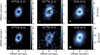 |
Fig. 1 Integrated-intensity maps of HCN isotopologs in the PDS 70 disk. The brightness temperatures were obtained assuming the Rayleigh-Jeans approximation. The HCN (4–3) map in the bottom right panel was obtained from SB observations alone. The white contours show the bright ring in the submillimeter continuum emission (Isella et al. 2019), the white dots mark the position of the two forming planets (2020 astrometry data from Wang et al. 2021), and the gray ellipse in the bottom left corner of each panel shows the synthesized beam. |
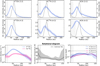 |
Fig. 2 Top panels: integrated-intensity profiles of lines of HCN isotopologs. The ribbons show the standard deviation across each annulus, divided by the square root of the number of independent beams. The intensity is expressed in brightness temperature under the Rayleigh-Jeans approximation. The dashed black line is the integrated-intensity profile of the 855 μm continuum (Isella et al. 2019; Benisty et al. 2021). The hatched region shows the beam major axis of each line. Bottom row: results of the radial rotational diagram analysis. The solid lines in the left and middle panels show the 50th percentile of the column density profiles (H13CN in blue and HC15N in pink) and of the excitation temperature (black). The ribbons show the 16th and 84th percentiles of the posterior distributions. The right panel represents the radial profiles of the optical depth for the analyzed molecular lines of H13CN and HC15N, and the related uncertainty is shown for the H13CN (3–2) line for reference because it is representative of the typical uncertainty. The dashed black line shows the τ = 1 level. |
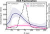 |
Fig. 3 Nitrogen (blue) and hydrogen (pink) fractionation profiles of HCN in the PDS 70 disk, assuming a radially constant 12C/13C = 69 value to convert the H13CN column density into an HCN column density. The ribbons indicate the 16th and 84th percentiles of the posterior distribution of the ratios. The dashed black line shows the integrated-intensity profile of the 855 μm continuum observations (Isella et al. 2019; Benisty et al. 2021). The hatched regions indicate the beam major axis of the data cubes of HCN isotopologs. |
3.2 Isotopolog ratios from fixed 12C/13C
The DCN/HCN and HCN/HC15N ratios in disks are usually extracted from H13CN instead of the main isotopolog HCN because the latter is typically optically thick (see, e.g., Guzmán et al. 2017). We also extracted the deuteration and nitrogen fractionation profiles by assuming a radially constant 12C/13C = 69 ratio (Wilson 1999) to convert the H13CN into an HCN column density. We therefore used the results of the rotational diagram analysis shown in Fig. 2, which we obtained from cubes by maximizing the sensitivity of the band 6 observations (see the second section of Table B.1 for the imaging specifics).
The posterior distributions of the 69 × N(H13CN)/N(HC15N) and N(DCN/[69 × N(H13CN)] ratios were built from the posterior distributions of the column density of H13CN, HC15N, and DCN. We reconstructed the posterior distribution of N(DCN) from Eq. (4) by randomly sampling the excitation temperature from the rotational diagram result, assuming that DCN has the same excitation temperature as H13CN and HC15N. The uncertainty on the DCN flux was accounted for in the posterior distribution of the isotopolog ratio by randomly sampling the flux of the DCN (3–2) line from a normal distribution centered around the median value, and the standard deviation was given by its statistical uncertainty. As for H13CN and HC15N, we extracted the radial profile of the DCN column density correcting for its optical depth using Eq. (5). The bottom row in Fig. D.1 in Appendix D shows the radial profiles of the DCN column density and optical depth compared to the other isotopologs.
The resulting radial profiles of the isotopolog ratios are presented in Fig. 3 and are also compared to the radial profile of the continuum-integrated intensity (dashed dark line), which lack any clear correlation with the fractionation profiles. The nitrogen fractionation profile decreases and is lower than the ISM value from ~40 to 100 au, while the deuteration profile is mostly constant between ~40 au 100 au and is significantly higher than the ISM D/H value of ~10−5 (Linsky et al. 2006).
3.3 Radial profile of the HCN column density
The radial profile of the HCN column density is needed to extract the HCN/H13CN ratio, or the HCN/HC15N and DCN/HCN ratios, without assuming a fixed 12C/13C ratio. The HCN column density, optical depth, and excitation temperature can be retrieved by leveraging the HCN hyperfine components, which are needed because the main component is typically optically thick, as previously presented by Guzmán et al. (2021) for the MAPS sample or by Hily-Blant et al. (2019) for the TW Hya disk.
However, the spatial resolution of SB observations of the HCN (4–3) line does not allow us to separate the two hyperfine components because beam smearing leads to a spatial blending of the hyperfine components. LB and SB observations of the analyzed data, on the other hand, allow us to spatially resolve the hyperfine component at 354.5075 GHz, centered at 3.8 km s−1 (main component vsys = 5.5 km s−1). As LB observations spectrally cover only one of the two hyperfine components and only half of the main component (see Fig. 4), we were unable to apply the rotational diagram to simultaneously extract the HCN column density and excitation temperature. We therefore computed the radial profile of the HCN column density, assuming the same excitation temperature as we obtained from the rotational diagram of H13CN and HC15N, through Eq. (1).
In particular, we reconstructed the HCN column density from the flux of the hyperfine component at 3.8 km s−1 by assuming that it is optically thin, which is valid since τ ≲ 0.02 from Eq. (5). To extract the radial profile of the flux of the hyperfine component, we applied a double-Gaussian fit to the spectrum in multiple radial bins. We fixed the center of the two Gaussian components at 3.8 km s−1 (hyperfine component) and at the systemic velocity of 5.5 km s−1 (main component), and we fit for the two widths and peaks. From the result of the Gaussian fit presented in Fig. 4, we then reconstructed the posterior distribution of the hyperfine flux, as outlined in Appendix D in more details.
We then reconstructed the posterior distributions of N(HCN) using Eqs. (1) and (2), from the reconstructed posterior distributions of the flux of the HCN hyperfine component and of the excitation temperature of H13CN and HC15N. In particular, we randomly sampled the excitation temperature from the result of the rotational diagram and the hyperfine flux from the posterior distribution obtained from the double-Gaussian fit.
We were unable to smooth the HCN cube to match the spatial resolution of ~![$\[0^{\prime\prime}_\cdot20\]$](/articles/aa/full_html/2025/06/aa54172-25/aa54172-25-eq19.png) of the H13CN and HC15N cubes used in the rotational diagram shown in Fig. 2 because a lower spatial resolution would deteriorate the hyperfine-fitting procedure because the hyperfine components are spectrally blended, as we outlined above. We therefore used the result from the rotational diagram shown in Appendix D, which we obtained from cubes with a higher spatial resolution of ~
of the H13CN and HC15N cubes used in the rotational diagram shown in Fig. 2 because a lower spatial resolution would deteriorate the hyperfine-fitting procedure because the hyperfine components are spectrally blended, as we outlined above. We therefore used the result from the rotational diagram shown in Appendix D, which we obtained from cubes with a higher spatial resolution of ~![$\[0^{\prime\prime}_\cdot15\]$](/articles/aa/full_html/2025/06/aa54172-25/aa54172-25-eq20.png) (see also Appendix B). The bottom left panel of Fig. D.1 in Appendix D shows the radial profiles of the HCN column density in comparison to the other isotopologs.
(see also Appendix B). The bottom left panel of Fig. D.1 in Appendix D shows the radial profiles of the HCN column density in comparison to the other isotopologs.
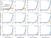 |
Fig. 4 Spectra of the HCN (4–3) line (dark blue lines) at different radii (indicated in the top right corner of each panel), with the related uncertainties. The dashed light blue line shows the fit to the spectrum as the sum of two Gaussian components. The orange profiles show the Gaussian fit to the hyperfine component, the dashed orange line corresponds to the 50th percentile of the posterior distribution, and the solid orange lines represent 100 random samples of the posterior distribution. |
3.4 Isotopolog ratios using the HCN column density
From the HCN column density retrieved from the hyperfine-fitting procedure, we extracted the radial profiles of the isotopolog ratios HCN/HC15N, HCN/H13CN, and DCN/HCN that are shown in Fig. 5 with the light blue, red, and purple profiles, respectively. Similarly to the previous case, where we fixed the 12C/13C ratio, the posterior distributions of the ratios were built from the posterior distributions of the column density of H13CN, HC15N (taken from the result of the rotational diagram shown in Fig. D.1), DCN, and HCN. As we described in Sect. 3.3, we used cubes that were imaged to maximize the sensitivity of the band 7 observations (see the first section of Table B.1 in Appendix B for imaging specifics) as a higher angular resolution is needed to perform the hyperfine-fitting procedure.
The middle panel of Fig. 5 shows that the carbon fractionation profile is consistent with the ISM value between ~50 and 100 au within the error bars. This also justifies the previous assumption we made of a radially constant 12C/13C to extract the deuteration and nitrogen fractionation profiles in Sect. 3.2 from the H13CN isotopolog. Moreover, the isotopolog ratios obtained by assuming a radially constant 12C/13C = 69 (dark blue and pink profiles in Fig. 5) or from the radial profile of the HCN column density directly (light blue and purple profiles) are consistent within the error bars.
The hyperfine-fitting procedure presented above and in Appendix D is strongly limited by the fact that only half of the HCN (4–3) line is covered by LB observations, by the low spectral resolution of ~0.9 km s−1, and by the lower signal to noise ratio. This consequently results in large error bars for the profiles of isotopolog ratios we obtained from the main isotopolog HCN, and it prevented us from robustly extracting the ratios inside ~40 au and beyond ~100 au.
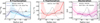 |
Fig. 5 Nitrogen, carbon, and hydrogen fractionation of the HCN molecule. Left panel: 69 × H13CN/HC15N (dark blue) and HCN/HC15N (light blue) profiles. Middle panel: HCN/H13CN. Right panel: 69 × H13CN/DCN (pink) and HCN/DCN (purple) profiles. Ribbons show the 16th and 84th percentiles of the posterior distributions of isotopolog ratios. The dashed horizontal black lines show the ISM values of 14N/15N = 274 (blue) and of 12C/13C = 69, and the ISM values of D/H are not indicated because they are ~10−5 (see references in Nomura et al. 2023). The marker length in each legend shows the major axis of the beam of cubes we used to retrieve the corresponding profiles in the plots. The dotted black line shows the 855 μm continuum integrated-intensity profile (Isella et al. 2019; Benisty et al. 2021). |
4 Discussion
4.1 Nitrogen
The isotope fractionation in disks is mainly driven by two processes: isotope exchange reactions, and isotope-selective photodissociation (Nomura et al. 2023, and references therein). For the specific case of nitrogen fractionation, the former can enhance the abundance of N15N and HC15N at low temperatures T ≲ 20 K (Terzieva & Herbst 2000). On the other hand, isotope-selective photodissociation of N15N over the self-shielding N2 is favored in strongly irradiated regions (Heays et al. 2014; Visser et al. 2018). It allows free 15N to enhance the HC15N abundance. This fractionation process is enhanced in strongly irradiated regions of the disk, such as the disk atmosphere or cavities of transition disks. Evidence of an efficient illumination of the PDS 70 cavity was presented by Law et al. (2024), along with its impact on the emission line morphology of various molecular tracers (Rampinelli et al. 2024). In this context, the radial profiles of isotope fractionation can reveal that different fractionation processes dominate at different planet-forming scales.
In particular, the radial profiles of 14N/15N were extracted for the disks around TW Hya (from CN and HCN isotopologs; Hily-Blant et al. 2017, 2019) and V4046 Sgr (from HCN isotopologs; Nomura et al. 2023, Guzmán et al., in prep.). The profiles were reconstructed up to ~60 au, and they both increase with radius, as shown in the left panel of Fig. 6. This was interpreted as the result of isotope-selective photodissociation: the higher gas density and stronger UV field at smaller radii result in an efficient self-shielding of N2 and in an efficient photodissociation of N15N, and thus, it results in enhanced HC15N in the inner region of the disks. These observational results also agree with fractionation models (Visser et al. 2018; Lee et al. 2021) and are consistent with the result we found for PDS 70 (see the left panel in Fig. 6). However, we highlight that the spatial resolution and sensitivity make the profiles shown in Figs. 3, 5, 6 highly uncertain for radii ≲25 au, and they therefore need to be interpreted with caution.
While the radial profiles of HCN/HC15N for TW Hya and V4046 Sgr only probe the increasing trend inside ~60 au, we were able to extract the isotopolog ratio out to ~120 au for the PDS 70 disk. The 14N/15N ratio shows a turnover at ~60 au, and it decreases below the ISM value at larger radii. This trend agrees with the predictions from the thermo-chemical models presented by Visser et al. (2018) for a typical disk around a T Tauri star (full disk). As they showed in their Fig. 12, the HCN/HC15N column density ratio is expected to increase to ~400 out to ~30 au and then decrease to ~260 between ~30 and 100 au. Visser et al. (2018) showed that the inner increase and outer decrease in the HCN/HC15N column density ratio are both the result of isotope-selective photodissociation of N2 because low-temperature isotope exchange reactions alone do not produce any strong radial variations: This qualitative agreement between the result directly extracted from ALMA observations in this work and the prediction from thermo-chemical models obtained assuming a typical disk around a T-Tauri star (Visser et al. 2018) suggests that regardless of the physical structure of the individual source that is analyzed, isotope-selective photodissociation plays a fundamental role in changing the HCN fractionation during the protoplanetary disk stage. This is also consistent with the fact that the decrease in HCN/HC15N in the outer disk is always HCN fractionation in disks predicted from thermo-chemical models by Visser et al. (2018), even when the disk parameters vary, such as the disk mass, flaring angle, large grain fraction, stellar type, or accretion rate.
The ratio of small to large grains has the strongest quantitative impact on the isotopolog ratio (Visser et al. 2018) because it affects the attenuation of UV photons, which cause the production and fractionation of HCN in the gas phase. The presence of an inner disk in the PDS 70 system, observed both in IR and submillimeter observations, and the large millimeter-dust cavity (~75 au) can therefore have a role in setting the fractionation levels of HCN and the radial location of the turn over in the HCN/HC15N profile (see the left panel in Fig. 6). In this context, both TW Hya and V4046 Sgr also show a dust cavity of ~2.5 au (Andrews et al. 2016) and ~13 au (Martinez-Brunner et al. 2022), respectively, which is smaller than the cavity of PDS 70, which also shows a deep gas gap. The location of the layer in which isotope-selective photodissociation dominates is also related to the distribution of the micrometer dust, which attenuates the UV flux. However, our attempt of extracting the HCN-emitting layer from the radial profile of its excitation temperature to compare it to the μm dust surface was inconclusive (see Appendix E). Specific thermo-chemical models for the PDS 70 disk are therefore needed to quantitatively reproduce the observed radial profile of the HCN/HC15N ratio.
We finally highlight that low-temperature isotope exchange reactions, even though they are less efficient than isotope-selective photodissociation (Roueff et al. 2015; Wirström & Charnley 2018; Loison et al. 2019), cannot be completely ruled out at low layers over the midplane or in the cold outer disk, outside the CO snowline (~70 au for the PDS 70 disk, as estimated by Law et al. 2024).
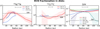 |
Fig. 6 Radial profiles of the nitrogen, carbon, and hydrogen fractionation of HCN in disks. The red profiles in the three panels show the results for the PDS 70 disk (solid lines and ribbons show the 50th, 16th, and 84th percentiles of the posterior distributions, respectively), and the horizontal dashed lines indicate the ISM values (Nomura et al. 2023; Ritchey et al. 2015; Wilson 1999; Linsky et al. 2006). The isotopic ratios profiles for the PDS 70 disk are compared to those for the TW Hya (Hily-Blant et al. 2019) and V4046 Sgr disks (Nomura et al. 2023, Guzmán et al., in prep.) for nitrogen in the left panel, the TW Hya disk (Hily-Blant et al. 2019) for carbon in the middle panel, and to the disks in the MAPS survey (Cataldi et al. 2021) for hydrogen in the right panel. The nitrogen and hydrogen fractionation profiles are obtained by converting the H13CN into an HCN column density, assuming a fixed 12C/13C = 69 ratio. The gray line at the top of each panel shows the major axis of the beam of the observations we used to extract the profiles for the PDS 70 disk. |
4.2 Carbon
The nitrogen fractionation of HCN shown in Fig. 3 was extracted assuming a radially constant 12C/13C equal to the ISM value, which makes the above interpretation only speculative because the role of nitrogen and carbon fractionation in determining the decreasing trend cannot be robustly distinguished with current observations. Nevertheless, our attempt of leveraging the HCN hyperfine component covered by the analyzed observations (see Appendix D) suggests that the HCN/H13CN ratio slightly increases between ~40 and 100 au, but the profile is consistent with the ISM value within the error bars. In this picture, the assumption of 12C/13C = 69 to convert the H13CN into an HCN column density is justified because the HCN/HC15N profile still shows a decreasing trend between ~40 and 90 au, which is consistent with the 69 × H13CN/HC15N profile.
To the best of our knowledge, the carbon isotopic ratio has only been extracted for one other disk, that is, the disk around TW Hya, for CO (Zhang et al. 2017; Yoshida et al. 2022), HCN (Hily-Blant et al. 2019), CN (Yoshida et al. 2024), and CCH (Bergin et al. 2024). These results showed that the value of 12C/13C can vary between ~20 to ~90 depending on the molecule used to extract it, and evidence for two separate carbon isotopic reservoirs was suggested (Bergin et al. 2024). The 12C/13C ratio extracted from HCN in TW Hya is shown in the middle panel of Fig. 6. HCN/H13CN is mostly constant and higher than the ISM value up to ~60 au.
On the other hand, our result for the PDS 70 disk shows that carbon fractionation may become relevant beyond ~90 au (see the middle panel of Fig. 5), which might be linked to the onset of the low-temperature isotope exchange reaction 13C + CO ⇄ C+ + 13CO + 35 K in the cold outer disk, which depletes 13C+ in favor of 13CO and increases the HCN/H13CN ratio (see, e.g., Visser et al. 2018; Öberg & Bergin 2021, and references therein). This result also qualitatively agrees with predictions from fractionation models performed by Visser et al. (2018) for HCN/H13CN. This can also affect the result we presented for the nitrogen and hydrogen fractionation in Fig. 3, which was extracted assuming a radially constant 12C/13C ratio. The low values of the 14N/15N and H/D ratios (dark blue and pink profiles in Fig. 3, respectively) outside ~100 au might be an artificial result of the assumption of a radially constant 12C/13C instead of nitrogen or hydrogen fractionation in the outer disk.
However, the picture of carbon fractionation is complex: Reactions that produce HCN can start either from C+ or C, depending on the region in the disk (Visser et al. 2018). Therefore, both low-temperature isotope exchange reactions and isotope-selective photodissociation can play a crucial role in determining the carbon fractionation of HCN. Moreover, these reactions primarily depend on the main C-carrier, that is, on CO, whose isotopic ratio should be inferred to better interpret the result for HCN. In this context, further thermochemical modeling that is specifically tuned on the transition disk of PDS 70 and higher spectral resolution observations that also fully cover the main and hyperfine components of the HCN (4–3) transition are needed to interpret the result for HCN fractionation and to robustly disentangle carbon and nitrogen fractionation.
4.3 Hydrogen
As for nitrogen fractionation, we extracted the deuteration profile of HCN either by N(DCN)/[N(H13CN) × 69] or by N(DCN)/N(HCN) (pink and purple line in the right panel of Fig. 5, respectively), and we used the resolved hyperfine component of the HCN line (see Appendix D). The deuteration profile is almost flat (~0.02 for radii between 40 and 100 au). The increase at ~100 au in the pink profile in the right panel of Fig. 5 might indicate a more efficient deuteration pathway in the cold outer disk, but the profile may be affected by carbon fractionation. The 12C/13C profile shown in Fig. 5 has large uncertainties outside ~90 au, and thus, it does not allow us to robustly conclude on the contribution of carbon fractionation in the outer disk. Similarly to the nitrogen fractionation, in order to definitely disentangle the effect of carbon fractionation, new high spectral resolution observations covering the two hyperfine components of the HCN line are needed.
The deuteration level of the HCN molecule in the PDS 70 disk is significantly higher than the ISM value of ~10−5 (Linsky et al. 2006; Nomura et al. 2023), which suggests that efficient deuteration processes enrich HCN with deuterium. The main deuteration pathway in protoplanetary disks is through isotope exchange reactions involving HD at low temperatures (T ≲ 25 K) or CH3+ at higher temperatures (T ≲ 300 K) (Millar et al. 1989; Aikawa & Herbst 1999; Stark et al. 1999), which produce H2D+ and CH2D+, respectively. Deuterium from H2D+and CH2D+ can be transferred to other molecules through proton transfer, such as HNC + H2D+ → DCNH+ + H2, which can subsequently produce DCN through dissociative recombination DCNH+ + e− → DCN + H (Cataldi et al. 2021).
Because the gas temperatures at which these reactions set differ, we expect them to dominate in different regions in the disk. The radial profile of DCN/HCN ratio is mostly constant at ~0.02 between ~40 and 100 au, which suggests that both reactions are important in setting the deuteration level of HCN, even if at different radial scales.
The right panel of Fig. 6 shows the comparison between the radial profile of HCN deuteration in the PDS 70 disk (red profile) and the MAPS survey (Cataldi et al. 2021). The D/H values show a large scatter among different sources, but they are systematically higher than the elemental ISM value (dashed horizontal black line). This suggests that in situ fractionation processes actively reset the original ISM value in a source-dependent way, which is strongly affected by different physical conditions set in different disks, such as the gas temperature or ionization structure. In particular, as resulting from the MAPS survey (Cataldi et al. 2021), the DCN/HCN profile in disks around Herbig stars show a steeper decreasing profile of DCN/HCN at small radii than T Tauri disks (see the right panel of Fig. 6). This has been interpreted as the effect of a higher temperature at small radii for Herbig than for T Tauri disks, which inhibits the deuteration reaction. This picture is consistent with the fact that the radial profile of the DCN/HCN ratio inside ~100 au for the T Tauri disk of PDS 70 is compatible with those for T Tauri disks in the MAPS sample.
4.4 Comparison with early and later stages
Fig. 7 shows a summary of nitrogen, carbon, and hydrogen fractionation of HCN in various astronomical objects at different evolutionary stages of star and planet formation from the literature. Appendix F lists all the references for the values presented in Fig. 7 and some details on the adopted methodologies.
The isotopolog ratios of HCN at early stages of the star formation history, that is, in prestellar cores and class 0/I young stellar objects (YSOs), are in most of the cases consistent with the results presented in this work for the PDS 70 disk. This suggests either a conservation of the original gas-phase isotopolog fractionation or indicates that if gas-phase fractionation processes are fast and the physical conditions in each stage are similar, the resulting isotopolog ratios are consistent. On the other hand, the HCN/HC15N and DCN/HCN ratios in prestellar or protostellar cores both show a large spread, which might highlight the strong dependence of the fractionation processes on the local physical condition in different sources, such as the gas temperature for isotope exchange reactions and the radiation field for isotope-selective photodissociation. Moreover, the HCN/HC15N values extracted for early stages presented in Fig. 7 include both direct and indirect methods that relied on various assumptions, such as the 12C/13C conversion factor, or the line opacities (Hily-Blant et al. 2020; Jensen et al. 2024, see also Appendix F). Hily-Blant et al. (2020) highlighted that indirect methods result in more scattered 14N/15N values than direct methods. In particular, the first direct estimates of HCN/H13CN and HCN/HC15N for a prestellar core were presented by Magalhães et al. (2018), who reported deviations from indirect methods that indicated a 13C enrichment. Similarly, Jensen et al. (2024) presented both direct and indirect measurements of the HCN/HC15N ratio toward six starless and prestellar cores that were significantly different (as also shown in Fig. 7). Consistent with our results above, Jensen et al. (2024) also reported no evident trend among different stages of star formation when considering direct estimates. It is also important to highlight that in the YSO phase, there could be a gas-phase contribution of HCN that is directly released from icy grains even when gas-phase formation of HCN is thought to be dominant (Bergner et al. 2020). The gas-phase origin of HCN in YSOs is supported by single-dish observations in which the HCN sublimation region (HCN desorption temperature of ~3370 K, Noble et al. 2012, Bergner et al. 2022) is unresolved (Cataldi et al. 2021). Finally, as shown in Fig. 7, Evans et al. (2022) presented the HCN/HC15N ratio measured in different regions of the protocluster OMC-2 FIR4. Their results for the central region is in line with the trend observed in YSOs, while they measure a higher ratio for the east region, which is more distant from the protocluster center. This again highlights the importance of studying spatial variations of fractionation levels in the same source because fractionation processes are strongly affected by the local physical conditions.
A spread of HCN/HC15N and DCN/HCN ratios was also observed in protoplanetary disks (PPDs) (Huang et al. 2017; Guzmán et al. 2017; Hily-Blant et al. 2019), with HCN/HC15N values that agree with measurements for early and later stages. DCN/HCN ratios show a difference of approximately an order of magnitude between disks around T Tauri and Herbig stars (Huang et al. 2017), with the lowest deuteration levels measured in Herbig disks, possibly because their temperature is higher than that of T Tauri disks, as we mentioned in Sect. 4.3. The T Tauri disk of V4046 Sgr is an exception in this picture, with its low value of DCN/HCN ~ 50, which is also only higher by a factor of ~2 than the DCN/HCN ratio measured for the Hale-Bopp comet (Meier et al. 1998). In this context, we highlight that V4046 Sgr is the oldest disk in the sample. It is ~23 Myr old (Mamajek & Bell 2014), and this might also affect its deuteration level. Moreover, we highlight that the HCN isotopolog ratios presented in Fig. 7 for protoplanetary disks are only disk integrated, while the radial variations presented in Fig. 6 reveal that the local environment affects the fractionation processes.
The HCN/H13CN ratios seem to suggest an increasing evolutionary trend. The ratios in early stages and comets match the HCN/H13CN values at small and large radii in the PDS 70 disk, respectively. On the other hand, the large uncertainties on the HCN/H13CN radial profile in the PDS 70 disk do not allow us to assess the robustness of this trend. Richer statistics of the carbon fractionation for early and later stages of star and planet formation and observations with a higher spectral resolution for the PDS 70 disk might both shed light on the origin of this possible trend.
For the comparison with later stages, we compared the HCN isotopolog ratios extracted for the PDS 70 disk with cometary values for Jupiter-family (JF) and Oort-family (OF) comets. The 12C/13C and 14N/15N ratios agree well with the values we found in the PDS 70 disk, especially with the outer disk region outside ~70 au, which seems to suggest a correlation between the cometary material and the gas-phase composition in the outer disk (Bockelée-Morvan et al. 2008; Cordiner et al. 2019). On the other hand, this picture is inconsistent with the only measurement of DCN/HCN in the Hale-Bopp comet, which is lower by approximately one order of magnitude than the PDS 70 disk values (Meier et al. 1998). Moreover, the DCN/HCN and HCN/H13CN ratios in comets are inconsistent with the corresponding ratios measured in prestellar and protostellar cores.
The low value of DCN/HCN in Hale-Bopp suggests that the HCN ice observed in the comet probably does not probe the same gas-phase HCN reservoir as observed in prestellar and protostellar cores. In particular, the ice component might originate from the early phases of star and planet formation. Due to the low formation efficiency of HCN ice, it is undetected in the ISM, although a low abundance is expected (Gerakines et al. 2004; Mumma & Charnley 2011; Gerakines et al. 2022; McClure et al. 2023). The cometary HCN deuteration might also have been altered after HCN was incorporated into the ice. In particular, thermally or radiation-induced exchange reactions on the ices were shown to play an important role in altering the deuteration of a variety of ices, such as hydrocarbon or methanol-water ices (Mousis et al. 2000; Weber et al. 2009; Faure et al. 2015).
In summary, we highlight that this is still a very uncertain picture and requires further investigation. In particular, better statistics on the DCN/HCN in comets might help us to understand whether the value measured for the Hale-Bopp comet is an outlier or typical for comets. The HCN fractionation is generally poorly constrained in comets, which makes it difficult to speculate about the origin. Moreover, further theoretical modeling and laboratory studies of HCN ices are needed to shed light on the role of deuteration in the ice phase. Similarly, it is important to probe the HCN carbon fractionation in more objects throughout the star and planet formation timeline to assess the suggested evolutionary trend.
Finally, we highlight that we were unable to compare our results with the recent measurements of isotopolog ratios in exoplanetary atmospheres directly (Zhang et al. 2021; Gandhi et al. 2023) because the latter are not obtained from the same tracers (NH3 and CO) as the former (HCN) and might therefore be driven by fractionation processes that are very different from those we probed with observations here.
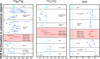 |
Fig. 7 Nitrogen, carbon, and hydrogen fractionation in various astronomical objects. The red and dark blue markers indicate the isotope ratios of HCN, and the red dots refer to values extracted at different radii for the PDS 70 disk in this work. The light blue markers show the isotopic ratios. The green marker in the middle panel for the Sun is obtained from CO. The dashed light blue lines refer to the ISM isotopic ratios (Linsky et al. 2006; Wilson 1999; Ritchey et al. 2015). No error bars are displayed when the uncertainty was too low to be visible in the plot. The squares indicate indirect measurements of DCN/HCN and HCN/HC15N ratios, assuming a fixed 12C/13C, and circles refer to results obtained directly from the main isotopolog HCN (see Appendix F for references for the values presented here and related methods). For a few sources, both direct and indirect estimates are available and are displayed in the same row, connected by dashed horizontal lines. The aligned empty squares refer to the ratios we extracted for the same source, but in different regions. |
5 Conclusion
We presented radial profiles of the carbon, nitrogen, and hydrogen fractionation of the HCN molecule in the planet-hosting disk around PDS 70 that showed that local fractionation pathways can alter isotopolog ratios. We summarize the main results below:
We showed spatially resolved emission of HCN (4–3), H13CN (3–2), H13CN (4–3), HC15N (3–2), HC15N (4–3), and DCN (3–2) in the PDS 70 disk.
We presented a decreasing trend of the 14N/15N isotopic ratio of HCN outside the disk cavity wall, which we suggested is linked to isotope-selective photodissociation of N2.
We showed that the D/H profile of HCN is almost flat throughout the disk and decreases slightly in the outer disk. The deuteration profile shows no correlation with the nitrogen fractionation profile, which is consistent with the fact that deuteration is thought to be mainly driven by gas-phase isotope-exchange reactions in the cold midplane or outer disk.
We retrieved the radial profile of the HCN/H13CN ratio by extracting the HCN column density, for which we used the spatially and spectrally resolved hyperfine component of HCN (4–3). The extracted 12C/13C ratio is consistent with the ISM value. This suggests that the decreasing trend in H13CN/HC15N is primarily driven by local nitrogen fractionation pathways.
The radial variations of the gas-phase isotopolog ratios reveal local fractionation pathways in the PDS 70 disk that might leave an imprint on the gas that is accreted by the two forming planets. This highlights the potential of isotopic ratios to reconstruct the journey of planetary material. Observations with a higher spectral resolution that also cover the high-velocity hyperfine component of the HCN line are needed to robustly confirm our results. Moreover, a comparison with thermochemical models that are specifically tuned on PDS 70 might help us to interpret observations in the light of possible fractionation pathways, and in particular, to better constrain the role of carbon fractionation in the main C-carrier, that is, of CO.
This work adds to the list of the few protoplanetary disks with a detailed analysis of their fractionation profiles. PDS 70 is the only target for which the photospheres of embedded protoplanets can be observed and characterized. Even though modeling is needed to connect the fractionation of different molecular or atomic species that best trace individual evolutionary steps in the star and planet formation process, it is of primary importance to promote a direct comparison of isotopolog ratios in exoplanetary atmospheres and protoplanetary disks to build a bridge between formed planets and their natal environment.
Acknowledgements
We thank V.V. Guzmán, P. Hily-Blant, and G. Cataldi for their availability in sharing results particularly important for the purpose of this work. This paper makes use of the following ALMA data: ADS/JAO.ALMA 2019.1.01619.S, ADS/JAO.ALMA 2022.1.01695.S. ALMA is a partnership of ESO (representing its member states), NSF (USA) and NINS (Japan), together with NRC (Canada), MOST and ASIAA (Taiwan), and KASI (Republic of Korea), in cooperation with the Republic of Chile. The Joint ALMA Observatory is operated by ESO, AUI/NRAO and NAOJ. L.R., S.F., and M.L. are funded by the European Union (ERC, UNVEIL, 101076613). Views and opinions expressed are however those of the authors only and do not necessarily reflect those of the European Union or the European Research Council. Neither the European Union nor the granting authority can be held responsible for them. S.F. also acknowledges financial contribution from PRIN-MUR 2022YP5ACE. P.C. acknowledges support by the ANID BASAL project FB210003. M.B. has received funding from the European Research Council (ERC) under the European Union’s Horizon 2020 research and innovation programme (PROTOPLANETS, grant agreement No. 101002188). Support for C.J.L. was provided by NASA through the NASA Hubble Fellowship grant No. HST-HF2-51535.001-A awarded by the Space Telescope Science Institute, which is operated by the Association of Universities for Research in Astronomy, Inc., for NASA, under contract NAS5-26555. B.P.R. is supported by NASA STScI grant JWST-GO-01759.002-A. The Center for Exoplanets and Habitable Worlds is supported by the Pennsylvania State University and the Eberly College of Science. The PI acknowledges the use of computing resources from the Italian node of the European ALMA Regional Center, hosted by INAF-Istituto di Radioastronomia.
Appendix A Fluxes of Band 6 and 7 molecular lines
The spectral set up of Band 7 data (2022.1.01695.S, PI M. Benisty) includes other molecular lines in addition to the HCN isotopologues ones: 12CO (3–2), CS (7–6), HCO+ (4–3), and SO (88−77). Rest frequencies, imaging parameters, and line fluxes of the detected molecular transitions are listed in Table A.1. Cubes were obtained using natural weighting. Line fluxes are obtained by spatially integrating the integrated-intensity maps of each line inside a de-projected circle with radius 3″ for the most extended 12CO, and 2″ for the others. The uncertainty is evaluated as the standard deviation of the flux measured in 26 de-projected circles, outside the emitting area of the integrated-intensity maps, with the same radius used to extract the flux. We took the maximum number of circles that was possible to place on the image without overlap, and used not primary beam corrected images, to ensure uniform noise (Rampinelli et al. 2024). Table A.1 lists also detected lines in Band 6 data (2019.1.01619.S, PI S. Facchini): the reader is referred to Rampinelli et al. (2024) for more details on imaging strategies and line flux evaluation.
Detected lines in Band 6 and 7 observations, rest frequencies, imaging properties (channel width, beam, RMS, and fluxes).
Appendix B Imaging procedure
To retrieve the radial profiles of nitrogen, carbon, and hydrogen fractionation of HCN, we performed two rounds of imaging to match the spatial resolution of Band 6 and 7 observations, respectively. We chose the robust and/or Gaussian uv-taper which resulted in cubes with beam areas as close as possible in the two cases. The imaging parameters used in the two cases, resulting beam sizes and areas, and RMS are listed in Tab. B.1. For the first case, only H13CN, HC15N, and DCN were imaged for the purpose of the analysis, while in the second case we also imaged the combined SB and LB observations of HCN. The resulting cube, with the corresponding beam size, beam area, and RMS listed in Tab. B.1 only covers half of the HCN (4-3) line.
Weighting, uv-taper, beam size, beam area, epsilon values, and RMS of imaged cubes used in the analysis.
Appendix C Spectral smearing effect on brightness temperature
In this work we evaluated the optical depth of the analysed lines starting from their peak brightness temperature and excitation temperature (see Eq. 5 in Sect. 3). However, the brightness temperature may be underestimated due to spectral smearing related to a finite spectral resolution. To quantitatively estimate the effect of spectral smearing we imaged the same cube of the H13CN (3-2) line twice, with a different channel width, and we extracted the radial profile of the peak brightness temperature, as shown in Fig. C.1. We compared the profiles starting from a cube with a channel width of 0.4 km s−1 (blue profile), which is the smallest channel width allowed by the spectral resolution, and of 0.8 km s−1 (red profile). As visible from Fig. C.1, a lower peak brightness temperature corresponds to a larger channel width. Moreover, spectral smearing dominates at larger radii, which is expected by the decreasing line width. At smaller radii the effect is smaller, and also negligible with respect to statistical uncertainties. We highlight that even at larger radii a 10% variation in the peak brightness temperature corresponds to roughly 1% variation in the upper level population, for an excitation temperature of ~30 K. This effect is thus negligible in the rotational diagram analysis we performed in this work.
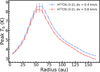 |
Fig. C.1 Radial profiles of peak brightness temperature extracted from cubes of the same H13CN (3-2) line, changing only the channel width in the imaging procedure (0.4 km s−1 blue line, 0.8 km s−1 red line). Error bars refer to the standard deviation of the brightness temperature in each annulus considered in the profile. |
Appendix D 12C/13C ratio from the HCN hyperfine component
The 14N/15N ratio of the HCN molecule in disks is typically extracted from H13CN and HC15N, assuming a fixed 12C/13C ratio to convert the H13CN column density into an HCN column density, as the main isotopologue HCN is generally optically thick (see, e.g., Guzmán et al. 2017). On the other hand, when hyperfine components of HCN are spectrally resolved, the HCN column density, optical depth and excitation temperature can be inferred, together with their radial profiles if hyperfine components are also spatially resolved (see, e.g., Hily-Blant et al. 2019; Guzmán et al. 2021). Long baseline observations of the HCN (4-3) line in the data we analysed only cover half of the main component spectrum, but they allow to resolve the hyperfine component at 354.5075 GHz. Figure 4 shows the HCN spectra (dark blue line) extracted averaging over annuli at different radii (indicated on the top right of each panel), corrected for the Keplerian rotation of the disk using the GoFish package (Teague 2019). Only half of the main component is covered (vsys = 5.5 km s−1), but the hyperfine component at 354.5075 GHz is marginally spectrally resolved (peak at v = 3.8 km s−1), even with a spectral resolution of ~0.9 km s−1. We extracted the flux associated with the hyperfine component by fitting a double Gaussian to the spectrum, stopping at 5.5 km s−1. We fixed the center of the two Gaussian components to 3.8 km s−1 for the hyperfine and to 5.5 km s−1 for the main component respectively, and fit for the two widths and peaks. We sampled the posterior distribution using an MCMC sampler through the emcee package (Foreman-Mackey et al. 2013). In order to take into account the spectral response, particularly critical for low spectral resolution, we spectrally over-sampled the Gaussian profiles and took the average value inside a spectral bin, to fit the observed spectrum. We applied the MCMC sampling to each annulus in which we divided the disk, with 128 walkers, 500 burn-in steps, and 500 steps, assuming a uniform prior of (0, 5) km s−1 for the two widths, of (0, 10) mJy beam−1 for the peak of the hyperfine component, and of (0, 30) mJy beam−1 for the peak of the main component.
Figure 4 shows the result of the MCMC sampling, for each annulus (the radius is indicated on the top right of each panel). The dashed light blue line is the sum of the two best fit Gaussian profiles, the dashed orange line shows the best fit Gaussian for the hyperfine component, the solid orange lines are 100 random samples of the posterior distribution, while the dark blue profile is the observed spectrum with the related uncertainty. The uncertainty for each spectrum was evaluated as standard deviation of the spectrum in a signal-free spectral range. We extracted the flux by integrating the Gaussian profiles of the hyperfine component obtained from the posterior distribution, with the best fit value being the 50th percentile of the posterior distribution of such fluxes, and the related uncertainty evaluated from the 16th and the 84th percentiles. From the flux of the hyperfine component, and the related uncertainty, we extracted the radial profile of the column density of HCN, assuming that the hyperfine component is optically thin, and the same excitation temperature inferred from the rotational diagram analysis of H13CN and HC15N. The fiducial radial range is between ~50 and 120 au, because for small radii the two components are blended, and the fit is poorly constrained, while for large radii the fit converges towards larger line widths, which are not physical. On the other hand, in the fiducial range the Gaussian fit to the hyperfine component is consistent with a radially constant line width. In this radial range, we extracted the 12C/13C profile shown in the middle panel of fig. 5, taking the ratio between the HCN and the H13CN column densities.
We could not smooth the HCN cube to match the spatial resolution of H13CN and HC15N Band 6 observations, as a worse spatial resolution would deteriorate the hyperfine fitting procedure (see also Sect. 3.3). We therefore imaged the Band 6 H13CN and HC15N cubes again with Briggs weighting and a robust parameter of 0.67 to match the spatial resolution of Band 7 observations. We then applied again the rotational diagram analysis, as shown in Sect. 3 and Fig. 2: the new result of the column density profiles and excitation temperatures are shown in Fig. D.1. Similarly, we re-imaged the DCN cube with a robust parameter of 0.3 to match the beam size of Band 7 observations, and extract the column density profile. Figure 5 shows the corresponding fractionation profiles.
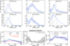 |
Fig. D.1 Same as Fig. 2, but with cubes imaged to match the beam size of the HCN cube obtained from SB+LB observations. The radial profile of the integrated intensity of HCN is extracted from the cube obtained only from SB observations. |
Appendix E HCN emitting layer from the excitation temperature
As we mentioned in Sect. 4.1, the distribution of the μm dust can influence the efficiency of isotope selective photodissociation of N2, as it attenuates UV photons. It could be therefore important to constrain the emitting layer height of HCN with respect to the small dust. We tried to retrieve the HCN emitting layer, by comparing the radial profile of the excitation temperature in Fig. 2 with the 2D temperature structure of the PDS 70 disk, extracted by Law et al. (2024), from CO isotopologues and HCO+. The rotational diagram assumes that the excitation temperature Tex(r) is equal to the kinetic temperature T(r, z) (LTE). We therefore inverted the T(r, z) relation (Law et al. 2024) to extract the emitting layer z(r) (see also Ilee et al. 2021; Rampinelli et al. 2024), assuming a geometrically thin emitting layer, and that the HCN excitation temperature is the same as the one obtained for H13CN and HC15N. The result is presented in Fig. E.1 (pink line), but the large uncertainties make it inconclusive.
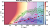 |
Fig. E.1 HCN emitting layer height as a function of radius (solid pink line), with the related uncertainty (pink ribbons), compared to the 2D temperature structure in the background (Law et al. 2024). The two solid green and blue lines refer to the 12CO and 13CO emission surfaces, with related uncertainties, respectively (Law et al. 2024). The dashed red line shows the NIR scale height as a function of radius, from Keppler et al. (2018), while the red diamond is the height of the NIR emitting layer at the NIR ring ~ |
![$\[0^{\prime\prime}_\cdot48\]$](/articles/aa/full_html/2025/06/aa54172-25/aa54172-25-eq55.png)
Appendix F HCN fractionation across the timeline of star and planet formation
A summary of the hydrogen, carbon, and nitrogen fractionation of HCN in various astronomical objects at different stages of star and planet formation is presented in Fig. 7.
DCN/HCN: The solar and ISM isotopic ratios are obtained from atomic hydrogen (Lodders 2003; Linsky et al. 2006). Hot core DCN/HCN ratios were extracted from observations taken with the Arizona Radio Observatory Submillimeter Telescope (SMT) (Gerner et al. 2015, HMC009.62, HMC010.47, HMC029.96, HMC045.47, HMC075.78, NGC7538B, Orion-KL, W3IRS5, W3H2 O). Column densities were extracted by correcting for the line optical depth, assuming the best-fit excitation temperature obtained from a 1D physico-chemical model with time-dependent D-chemistry (Gerner et al. 2015). We highlight that these results are in tension with DCN/HCN ratios previously extracted for the same sources by Hatchell et al. (1998), from DCN and HC15N observations taken with the James Clerk Maxwell Telescope, which result in DCN/HCN values up to approximately an order of magnitude lower than the ones presented by Gerner et al. (2015). The five DCN/HCN values presented for class 0/I sources (Bergner et al. 2020, Ser-emb 1,7,8,15,17) were obtained from ALMA observations, evaluating HCN column densities from H13CN, assuming an ISM 12C/13C, Tex = 30 K, and co-spatial emission from the different isotopologues. Disk integrated values of DCN/HCN were extracted for the protoplanetary disks of AS 209, IM Lup, V4046 Sgr, LkCa 15, and HD 163296 from ALMA observations of H13CN and DCN (Huang et al. 2017). The only DCN/HCN ratio measured for comets was obtained from James Clerk Maxwell Telescope observations of the Hale-Bopp comet (Meier et al. 1998). The deuteration level was measured from the line ratios of DCN and H13CN, assuming a solar 12C/13C, but also directly from the main isotopologue HCN, by correcting for its optical depth through the hyperfine components, leading to consistent results.
HCN/H13CN: The ISM isotope ratio was obtained from atomic carbon (Wilson 1999), while the solar value was obtained from CO (Lyons et al. 2018). HCN/H13CN ratios were extracted for the prestellar core Bernard 1b (Daniel et al. 2013), L1498 (Magalhães et al. 2018), the six starless and prestellar cores CB23, TMC2, L1495, L1495AN, L1512, and L1517B (Jensen et al. 2024) and the class 0 YSO L483 (Agúndez et al. 2019) from IRAM observations. The HCN/H13CN value for the disk around TW Hya was extracted from ALMA observations (Hily-Blant et al. 2019). Cometary HCN/H13CN ratios were obtained for Hale-Bopp (Bockelée-Morvan et al. 2008) from Harlan J. Smith Telescope observations, and for C/2012 S1 ISON (Cordiner et al. 2019) from ALMA observations leveraging the hyperfine components of the observed HCN line.
HCN/HC15N: The solar and ISM isotopic ratios were obtained from atomic nitrogen (Marty 2012; Ritchey et al. 2015). The prestellar/protostellar values are taken from Hily-Blant et al. (2020). The first direct measurement of HCN/HC15N was extracted for the prestellar core L1498 (Magalhães et al. 2018) and subsequently for the six starless and prestellar cores CB23, TMC2, L1495, L1495AN, L1512, and L1517B (Jensen et al. 2024), using a 1D radiative transfer code handling hyperfine overlap. The remaining HCN/HC15N values for prestellar cores L183, L1544 (Hily-Blant et al. 2013), L1521E (Ikeda et al. 2002), protocluster OMC-2 FIR4 (Evans et al. 2022), and class 0/I YSOs FIR3 (Evans et al. 2022), L1527 (Yoshida et al. 2019), IRAS 16293A, OMC-3, R CrA IRS7B (Wampfler et al. 2014), I-04365, I-04016, I-04166, I-04169, I-04181 (Le Gal et al. 2020), Ser-emb 1, 7, 8, 15, 17 (Bergner et al. 2020) were obtained from a so-called double-isotope indirect method, assuming a fixed 12C/13C ratio. The only direct measurement of the HCN/HC15N ratio in protoplanetary disks was obtained for the disk around TW Hya (Hily-Blant et al. 2019), while for the disks around AS 209, LkCa 15, and V4046 Sgr it was obtained from ALMA observations of H13CN and HC15N and assuming an ISM 12C/13C ratio (Guzmán et al. 2017). Cometary HCN/HC15N were presented for 17P/Holmes and Hale-Bopp (Bockelée-Morvan et al. 2008) from IRAM, Harlan J. Smith, and Keck telescopes observations, and leveraging the hyperfine components of the observed HCN line.
References
- Agúndez, M., Marcelino, N., Cernicharo, J., Roueff, E., & Tafalla, M. 2019, A&A, 625, A147 [Google Scholar]
- Ahrens, V., & Winnewisser, G. 1999, Zeitsch. Naturfor. A, 54, 131 [Google Scholar]
- Ahrens, V., Lewen, F., Takano, S., et al. 2002, Zeitsch. Naturfor. A, 57, 669 [Google Scholar]
- Aikawa, Y., & Herbst, E. 1999, ApJ, 526, 314 [Google Scholar]
- Albertsson, T., Semenov, D., & Henning, T. 2014, ApJ, 784, 39 [NASA ADS] [CrossRef] [Google Scholar]
- Aléon, J. 2010, ApJ, 722, 1342 [CrossRef] [Google Scholar]
- Altwegg, K., Balsiger, H., & Fuselier, S. A. 2019, ARA&A, 57, 113 [NASA ADS] [CrossRef] [Google Scholar]
- Andrews, S. M., Wilner, D. J., Zhu, Z., et al. 2016, ApJ, 820, L40 [Google Scholar]
- Andrews, S. M., Huang, J., Pérez, L. M., et al. 2018, ApJ, 869, L41 [NASA ADS] [CrossRef] [Google Scholar]
- Barrado, D., Mollière, P., Patapis, P., et al. 2023, Nature, 624, 263 [NASA ADS] [CrossRef] [Google Scholar]
- Benisty, M., Bae, J., Facchini, S., et al. 2021, ApJ, 916, L2 [NASA ADS] [CrossRef] [Google Scholar]
- Benisty, M., Dominik, C., Follette, K., et al. 2023, in Astronomical Society of the Pacific Conference Series, 534, Protostars and Planets VII, eds. S. Inutsuka, Y. Aikawa, T. Muto, K. Tomida, & M. Tamura, 605 [Google Scholar]
- Bergin, E. A., Bosman, A., Teague, R., et al. 2024, ApJ, 965, 147 [NASA ADS] [CrossRef] [Google Scholar]
- Bergner, J. B., Öberg, K. I., Bergin, E. A., et al. 2020, ApJ, 898, 97 [NASA ADS] [CrossRef] [Google Scholar]
- Bergner, J. B., Rajappan, M., & Öberg, K. I. 2022, ApJ, 933, 206 [Google Scholar]
- Bockelée-Morvan, D., Biver, N., Jehin, E., et al. 2008, ApJ, 679, L49 [CrossRef] [Google Scholar]
- Bogey, M., Demuynck, C., & Destombes, J. 1981, Chem. Phys. Lett., 81, 256 [NASA ADS] [CrossRef] [Google Scholar]
- Bogey, M., Demuynck, C., & Destombes, J. 1986, Chem. Phys. Lett., 125, 383 [NASA ADS] [CrossRef] [Google Scholar]
- Booth, A. S., Ilee, J. D., Walsh, C., et al. 2023, A&A, 669, A53 [Google Scholar]
- Brünken, S., Fuchs, U., Lewen, F., et al. 2004, J. Mol. Spectrosc., 225, 152 [CrossRef] [Google Scholar]
- CASA Team (Bean, B., et al.) 2022, PASP, 134, 114501 [NASA ADS] [CrossRef] [Google Scholar]
- Casassus, S., & Cárcamo, M. 2022, MNRAS, 513, 5790 [NASA ADS] [CrossRef] [Google Scholar]
- Cataldi, G., Yamato, Y., Aikawa, Y., et al. 2021, ApJS, 257, 10 [NASA ADS] [CrossRef] [Google Scholar]
- Cazzoli, G., & Puzzarini, C. 2005, J. Mol. Spectrosc., 233, 280 [NASA ADS] [CrossRef] [Google Scholar]
- Cazzoli, G., Puzzarini, C., & Lapinov, A. V. 2004, ApJ, 611, 615 [NASA ADS] [CrossRef] [Google Scholar]
- Ceccarelli, C., Caselli, P., Bockelée-Morvan, D., et al. 2014, in Protostars and Planets VI, eds. H. Beuther, R. S. Klessen, C. P. Dullemond, & T. Henning, 859 [Google Scholar]
- Chardon, J., & Guichon, D. 1973, J. Phys., 34, 791 [CrossRef] [EDP Sciences] [Google Scholar]
- Cleeves, L. I., Bergin, E. A., & Harries, T. J. 2015, ApJ, 807, 2 [NASA ADS] [CrossRef] [Google Scholar]
- Cordiner, M. A., Palmer, M. Y., de Val-Borro, M., et al. 2019, ApJ, 870, L26 [Google Scholar]
- Cornwell, T. J. 2008, IEEE J. Selected Top. Signal Process., 2, 793 [NASA ADS] [CrossRef] [Google Scholar]
- Cridland, A. J., van Dishoeck, E. F., Alessi, M., & Pudritz, R. E. 2020, A&A, 642, A229 [NASA ADS] [CrossRef] [EDP Sciences] [Google Scholar]
- Cridland, A. J., Facchini, S., van Dishoeck, E. F., & Benisty, M. 2023, A&A, 674, A211 [NASA ADS] [CrossRef] [EDP Sciences] [Google Scholar]
- Czekala, I., Loomis, R. A., Teague, R., et al. 2021, ApJS, 257, 2 [NASA ADS] [CrossRef] [Google Scholar]
- Daniel, F., Gérin, M., Roueff, E., et al. 2013, A&A, 560, A3 [NASA ADS] [CrossRef] [EDP Sciences] [Google Scholar]
- Drazkowska, J., Bitsch, B., Lambrechts, M., et al. 2023, in Astronomical Society of the Pacific Conference Series, 534, Protostars and Planets VII, eds. S. Inutsuka, Y. Aikawa, T. Muto, K. Tomida, & M. Tamura, 717 [Google Scholar]
- Evans, L., Fontani, F., Vastel, C., et al. 2022, A&A, 657, A136 [NASA ADS] [CrossRef] [EDP Sciences] [Google Scholar]
- Facchini, S., Teague, R., Bae, J., et al. 2021, AJ, 162, 99 [NASA ADS] [CrossRef] [Google Scholar]
- Faure, A., Faure, M., Theulé, P., Quirico, E., & Schmitt, B. 2015, A&A, 584, A98 [NASA ADS] [CrossRef] [EDP Sciences] [Google Scholar]
- Foreman-Mackey, D., Conley, A., Meierjurgen Farr, W., et al. 2013, emcee: The MCMC Hammer, Astrophysics Source Code Library [record ascl:1303.002] [Google Scholar]
- Fuchs, U., Bruenken, S., Fuchs, G. W., et al. 2004, Zeitsch. Naturfor. A, 59, 861 [Google Scholar]
- Furuya, K., Tsukagoshi, T., Qi, C., et al. 2022, ApJ, 926, 148 [NASA ADS] [CrossRef] [Google Scholar]
- Gaia Collaboration (Brown, A. G. A., et al.) 2018, A&A, 616, A1 [NASA ADS] [CrossRef] [EDP Sciences] [Google Scholar]
- Gandhi, S., de Regt, S., Snellen, I., et al. 2023, ApJ, 957, L36 [NASA ADS] [CrossRef] [Google Scholar]
- Gerakines, P., Moore, M., & Hudson, R. 2004, Icarus, 170, 202 [Google Scholar]
- Gerakines, P. A., Yarnall, Y. Y., & Hudson, R. L. 2022, MNRAS, 509, 3515 [Google Scholar]
- Gerner, T., Shirley, Y. L., Beuther, H., et al. 2015, A&A, 579, A80 [NASA ADS] [CrossRef] [EDP Sciences] [Google Scholar]
- Goldsmith, P. F., & Langer, W. D. 1999, ApJ, 517, 209 [Google Scholar]
- Gregersen, E. M., & Evans, Neal J., I. 2001, ApJ, 553, 1042 [NASA ADS] [CrossRef] [Google Scholar]
- Guzmán, V., Öberg, K., Loomis, R., & Qi, C. 2015, ApJ, 814, 53 [CrossRef] [Google Scholar]
- Guzmán, V. V., Öberg, K. I., Huang, J., Loomis, R., & Qi, C. 2017, ApJ, 836, 30 [Google Scholar]
- Guzmán, V. V., Bergner, J. B., Law, C. J., et al. 2021, ApJS, 257, 6 [CrossRef] [Google Scholar]
- Haffert, S. Y., Bohn, A. J., de Boer, J., et al. 2019, Nat. Astron., 3, 749 [Google Scholar]
- Hatchell, J., Millar, T. J., & Rodgers, S. D. 1998, A&A, 332, 695 [NASA ADS] [Google Scholar]
- Heays, A. N., Visser, R., Gredel, R., et al. 2014, A&A, 562, A61 [NASA ADS] [CrossRef] [EDP Sciences] [Google Scholar]
- Hily-Blant, P., Bonal, L., Faure, A., & Quirico, E. 2013, Icarus, 223, 582 [Google Scholar]
- Hily-Blant, P., Magalhaes, V., Kastner, J., et al. 2017, A&A, 603, L6 [NASA ADS] [CrossRef] [EDP Sciences] [Google Scholar]
- Hily-Blant, P., Magalhaes de Souza, V., Kastner, J., & Forveille, T. 2019, A&A, 632, L12 [NASA ADS] [CrossRef] [EDP Sciences] [Google Scholar]
- Hily-Blant, P., Pineau des Forêts, G., Faure, A., & Flower, D. R. 2020, A&A, 643, A76 [NASA ADS] [CrossRef] [EDP Sciences] [Google Scholar]
- Högbom, J. A. 1974, A&AS, 15, 417 [Google Scholar]
- Hsu, C.-C., Wang, J. J., Blake, G. A., et al. 2024, ApJ, 977, L47 [Google Scholar]
- Huang, J., Öberg, K. I., Qi, C., et al. 2017, ApJ, 835, 231 [Google Scholar]
- Ikeda, M., Hirota, T., & Yamamoto, S. 2002, ApJ, 575, 250 [NASA ADS] [CrossRef] [Google Scholar]
- Ilee, J. D., Walsh, C., Booth, A. S., et al. 2021, ApJS, 257, 9 [NASA ADS] [CrossRef] [Google Scholar]
- Isella, A., Benisty, M., Teague, R., et al. 2019, ApJ, 879, L25 [Google Scholar]
- Izquierdo, A. F., Testi, L., Facchini, S., et al. 2023, A&A, 674, A113 [NASA ADS] [CrossRef] [EDP Sciences] [Google Scholar]
- Jensen, S. S., Spezzano, S., Caselli, P., et al. 2024, A&A, 685, A149 [NASA ADS] [CrossRef] [EDP Sciences] [Google Scholar]
- Jiang, H., Wang, Y., Ormel, C. W., Krijt, S., & Dong, R. 2023, A&A, 678, A33 [NASA ADS] [CrossRef] [EDP Sciences] [Google Scholar]
- Jorsater, S., & van Moorsel, G. A. 1995, AJ, 110, 2037 [Google Scholar]
- Keppler, M., Benisty, M., Müller, A., et al. 2018, A&A, 617, A44 [NASA ADS] [CrossRef] [EDP Sciences] [Google Scholar]
- Keppler, M., Teague, R., Bae, J., et al. 2019, A&A, 625, A118 [NASA ADS] [CrossRef] [EDP Sciences] [Google Scholar]
- Klapper, G., Lewen, F., Gendriesch, R., Belov, S., & Winnewisser, G. 2000, J. Mol. Spectrosc., 201, 124 [NASA ADS] [CrossRef] [Google Scholar]
- Lattanzi, V., Walters, A., Drouin, B. J., & Pearson, J. C. 2007, ApJ, 662, 771 [NASA ADS] [CrossRef] [Google Scholar]
- Law, C. J., Booth, A. S., & Öberg, K. I. 2023, ApJ, 952, L19 [NASA ADS] [CrossRef] [Google Scholar]
- Law, C. J., Benisty, M., Facchini, S., et al. 2024, ApJ, 964, 190 [NASA ADS] [CrossRef] [Google Scholar]
- Lee, S., Nomura, H., Furuya, K., & Lee, J.-E. 2021, ApJ, 908, 82 [NASA ADS] [CrossRef] [Google Scholar]
- Leemker, M., Booth, A. S., van Dishoeck, E. F., Wölfer, L., & Dent, B. 2024, A&A, 687, A299 [NASA ADS] [CrossRef] [EDP Sciences] [Google Scholar]
- Le Gal, R., Öberg, K. I., Huang, J., et al. 2020, ApJ, 898, 131 [Google Scholar]
- Linsky, J. L., Draine, B. T., Moos, H. W., et al. 2006, ApJ, 647, 1106 [Google Scholar]
- Lodders, K. 2003, ApJ, 591, 1220 [Google Scholar]
- Loison, J.-C., Wakelam, V., Gratier, P., & Hickson, K. M. 2019, MNRAS, 484, 2747 [NASA ADS] [CrossRef] [Google Scholar]
- Loomis, R. A., Cleeves, L. I., Öberg, K. I., et al. 2018, ApJ, 859, 131 [Google Scholar]
- Loomis, R. A., Facchini, S., Benisty, M., et al. 2025, ApJ, 984, L7 [Google Scholar]
- Lovas, F. J., Suenram, R., Ogata, T., & Yamamoto, S. 1992, ApJ, 399, 325 [CrossRef] [Google Scholar]
- Lyons, J. R., Gharib-Nezhad, E., & Ayres, T. R. 2018, in 49th Annual Lunar and Planetary Science Conference, Lunar and Planetary Science Conference, 2907 [Google Scholar]
- Magalhães, V. S., Hily-Blant, P., Faure, A., Hernandez-Vera, M., & Lique, F. 2018, A&A, 615, A52 [NASA ADS] [CrossRef] [EDP Sciences] [Google Scholar]
- Maiwald, F., Lewen, F., Ahrens, V., et al. 2000, J. Mol. Spectrosc., 1, 166 [NASA ADS] [CrossRef] [Google Scholar]
- Mamajek, E. E., & Bell, C. P. M. 2014, MNRAS, 445, 2169 [Google Scholar]
- Martinez-Brunner, R., Casassus, S., Pérez, S., et al. 2022, MNRAS, 510, 1248 [Google Scholar]
- Marty, B. 2012, Earth Planet. Sci. Lett., 313, 56 [NASA ADS] [CrossRef] [Google Scholar]
- McClure, M. K., Rocha, W., Pontoppidan, K., et al. 2023, Nat. Astron., 7, 431 [NASA ADS] [CrossRef] [Google Scholar]
- Meier, R., Owen, T. C., Jewitt, D. C., et al. 1998, Science, 279, 1707 [Google Scholar]
- Millar, T. J., Bennett, A., & Herbst, E. 1989, ApJ, 340, 906 [NASA ADS] [CrossRef] [Google Scholar]
- Morbidelli, A., Chambers, J., Lunine, J. I., et al. 2000, Meteor. Planet. Sci., 35, 1309 [NASA ADS] [CrossRef] [Google Scholar]
- Mousis, O., Gautier, D., Bockelée-Morvan, D., et al. 2000, Icarus, 148, 513 [NASA ADS] [CrossRef] [Google Scholar]
- Müller, H. S. P., & Lewen, F. 2017, J. Mol. Spectrosc., 331, 28 [CrossRef] [Google Scholar]
- Müller, H. S. P., Klaus, T., & Winnewisser, G. 2000, A&A, 357, L65 [NASA ADS] [Google Scholar]
- Müller, H. S., Schlöder, F., Stutzki, J., & Winnewisser, G. 2005, J. Mol. Struct., 742, 215 [Google Scholar]
- Mumma, M. J., & Charnley, S. B. 2011, ARA&A, 49, 471 [NASA ADS] [CrossRef] [Google Scholar]
- Noble, J. A., Theule, P., Mispelaer, F., et al. 2012, A&A, 543, A5 [NASA ADS] [CrossRef] [EDP Sciences] [Google Scholar]
- Nomura, H., Furuya, K., Cordiner, M. A., et al. 2023, in Astronomical Society of the Pacific Conference Series, 534, Protostars and Planets VII, eds. S. Inutsuka, Y. Aikawa, T. Muto, K. Tomida, & M. Tamura, 1075 [Google Scholar]
- Öberg, K. I., & Bergin, E. A. 2021, Phys. Rep., 893, 1 [Google Scholar]
- Öberg, K. I., Murray-Clay, R., & Bergin, E. A. 2011, ApJ, 743, L16 [Google Scholar]
- Öberg, K. I., Qi, C., Wilner, D. J., & Hogerheijde, M. R. 2012, ApJ, 749, 162 [Google Scholar]
- Öberg, K. I., Facchini, S., & Anderson, D. E. 2023, ARA&A, 61, 287 [CrossRef] [Google Scholar]
- Okuzumi, S., & Tazaki, R. 2019, ApJ, 878, 132 [Google Scholar]
- Padovani, M., Walmsley, C., Tafalla, M., Galli, D., & Müller, H. 2009, A&A, 505, 1199 [NASA ADS] [CrossRef] [EDP Sciences] [Google Scholar]
- Perez, S., Dunhill, A., Casassus, S., et al. 2015, ApJ, 811, L5 [NASA ADS] [CrossRef] [Google Scholar]
- Pinte, C., Teague, R., Flaherty, K., et al. 2023, in Astronomical Society of the Pacific Conference Series, 534, Protostars and Planets VII, ed. S. Inutsuka, Y. Aikawa, T. Muto, K. Tomida, & M. Tamura, 645 [Google Scholar]
- Portilla-Revelo, B., Kamp, I., Facchini, S., et al. 2023, A&A, 677, A76 [NASA ADS] [CrossRef] [EDP Sciences] [Google Scholar]
- Rampinelli, L., Facchini, S., Leemker, M., et al. 2024, A&A, 689, A65 [NASA ADS] [CrossRef] [EDP Sciences] [Google Scholar]
- Ritchey, A. M., Federman, S. R., & Lambert, D. L. 2015, ApJ, 804, L3 [NASA ADS] [CrossRef] [Google Scholar]
- Roueff, E., Loison, J. C., & Hickson, K. M. 2015, A&A, 576, A99 [NASA ADS] [CrossRef] [EDP Sciences] [Google Scholar]
- Sastry, K., Helminger, P., Charo, A., Herbst, E., & De Lucia, F. 1981, ApJ, 251, L119 [NASA ADS] [CrossRef] [Google Scholar]
- Sierra, A., Pérez, L. M., Zhang, K., et al. 2021, ApJS, 257, 14 [NASA ADS] [CrossRef] [Google Scholar]
- Smith, R. L., Pontoppidan, K. M., Young, E. D., Morris, M. R., & van Dishoeck, E. F. 2009, ApJ, 701, 163 [Google Scholar]
- Stark, R., van der Tak, F. F. S., & van Dishoeck, E. F. 1999, ApJ, 521, L67 [NASA ADS] [CrossRef] [Google Scholar]
- Teague, R. 2019, J. Open Source Softw., 4, 1632 [NASA ADS] [CrossRef] [Google Scholar]
- Teague, R., & Foreman-Mackey, D. 2019, bettermoments: Line-of-sight velocity calculation, Astrophysics Source Code Library [record ascl:1901.009] [Google Scholar]
- Terzieva, R., & Herbst, E. 2000, MNRAS, 317, 563 [Google Scholar]
- Tinti, F., Bizzocchi, L., Degli Esposti, C., & Dore, L. 2007, ApJ, 669, L113 [NASA ADS] [CrossRef] [Google Scholar]
- Visser, R., Bruderer, S., Cazzoletti, P., et al. 2018, A&A, 615, A75 [NASA ADS] [CrossRef] [EDP Sciences] [Google Scholar]
- Vrtilek, J., Gottlieb, C., & Thaddeus, P. 1987, ApJ, 314, 716 [CrossRef] [Google Scholar]
- Wampfler, S. F., Jørgensen, J. K., Bizzarro, M., & Bisschop, S. E. 2014, A&A, 572, A24 [NASA ADS] [CrossRef] [EDP Sciences] [Google Scholar]
- Wang, J. J., Vigan, A., Lacour, S., et al. 2021, AJ, 161, 148 [Google Scholar]
- Weber, A. S., Hodyss, R., Johnson, P. V., Willacy, K., & Kanik, I. 2009, ApJ, 703, 1030 [Google Scholar]
- Wilson, T. L. 1999, Rep. Progr. Phys., 62, 143 [CrossRef] [Google Scholar]
- Winnewisser, M., Winnewisser, B. P., & Winnewisser, G. 1985, in NATO Advanced Study Institute (ASI) Series C, 157, eds. G. H. F. Diercksen, W. F. Huebner, & P. W. Langhoff, 375 [Google Scholar]
- Winnewisser, G., Belov, S., Klaus, T., & Schieder, R. 1997, J. Mol. Spectrosc., 184, 468 [NASA ADS] [CrossRef] [Google Scholar]
- Wirström, E. S., & Charnley, S. B. 2018, MNRAS, 474, 3720 [CrossRef] [Google Scholar]
- Yoshida, K., Sakai, N., Nishimura, Y., et al. 2019, PASJ, 71, S18 [NASA ADS] [CrossRef] [Google Scholar]
- Yoshida, T. C., Nomura, H., Furuya, K., Tsukagoshi, T., & Lee, S. 2022, ApJ, 932, 126 [NASA ADS] [CrossRef] [Google Scholar]
- Yoshida, T. C., Nomura, H., Furuya, K., et al. 2024, ApJ, 966, 63 [Google Scholar]
- Zhang, K., Bergin, E. A., Blake, G. A., Cleeves, L. I., & Schwarz, K. R. 2017, Nat. Astron., 1, 0130 [NASA ADS] [CrossRef] [Google Scholar]
- Zhang, Y., Snellen, I. A. G., Bohn, A. J., et al. 2021, Nature, 595, 370 [NASA ADS] [CrossRef] [Google Scholar]
- Zhou, Y., Bowler, B. P., Wagner, K. R., et al. 2021, AJ, 161, 244 [NASA ADS] [CrossRef] [Google Scholar]
All Tables
Listed imaged lines, corresponding rest frequencies, line properties, and imaging parameters (channel width, beam, and RMS).
Detected lines in Band 6 and 7 observations, rest frequencies, imaging properties (channel width, beam, RMS, and fluxes).
Weighting, uv-taper, beam size, beam area, epsilon values, and RMS of imaged cubes used in the analysis.
All Figures
|
Fig. 1 Integrated-intensity maps of HCN isotopologs in the PDS 70 disk. The brightness temperatures were obtained assuming the Rayleigh-Jeans approximation. The HCN (4–3) map in the bottom right panel was obtained from SB observations alone. The white contours show the bright ring in the submillimeter continuum emission (Isella et al. 2019), the white dots mark the position of the two forming planets (2020 astrometry data from Wang et al. 2021), and the gray ellipse in the bottom left corner of each panel shows the synthesized beam. |
| In the text | |
|
Fig. 2 Top panels: integrated-intensity profiles of lines of HCN isotopologs. The ribbons show the standard deviation across each annulus, divided by the square root of the number of independent beams. The intensity is expressed in brightness temperature under the Rayleigh-Jeans approximation. The dashed black line is the integrated-intensity profile of the 855 μm continuum (Isella et al. 2019; Benisty et al. 2021). The hatched region shows the beam major axis of each line. Bottom row: results of the radial rotational diagram analysis. The solid lines in the left and middle panels show the 50th percentile of the column density profiles (H13CN in blue and HC15N in pink) and of the excitation temperature (black). The ribbons show the 16th and 84th percentiles of the posterior distributions. The right panel represents the radial profiles of the optical depth for the analyzed molecular lines of H13CN and HC15N, and the related uncertainty is shown for the H13CN (3–2) line for reference because it is representative of the typical uncertainty. The dashed black line shows the τ = 1 level. |
| In the text | |
|
Fig. 3 Nitrogen (blue) and hydrogen (pink) fractionation profiles of HCN in the PDS 70 disk, assuming a radially constant 12C/13C = 69 value to convert the H13CN column density into an HCN column density. The ribbons indicate the 16th and 84th percentiles of the posterior distribution of the ratios. The dashed black line shows the integrated-intensity profile of the 855 μm continuum observations (Isella et al. 2019; Benisty et al. 2021). The hatched regions indicate the beam major axis of the data cubes of HCN isotopologs. |
| In the text | |
|
Fig. 4 Spectra of the HCN (4–3) line (dark blue lines) at different radii (indicated in the top right corner of each panel), with the related uncertainties. The dashed light blue line shows the fit to the spectrum as the sum of two Gaussian components. The orange profiles show the Gaussian fit to the hyperfine component, the dashed orange line corresponds to the 50th percentile of the posterior distribution, and the solid orange lines represent 100 random samples of the posterior distribution. |
| In the text | |
|
Fig. 5 Nitrogen, carbon, and hydrogen fractionation of the HCN molecule. Left panel: 69 × H13CN/HC15N (dark blue) and HCN/HC15N (light blue) profiles. Middle panel: HCN/H13CN. Right panel: 69 × H13CN/DCN (pink) and HCN/DCN (purple) profiles. Ribbons show the 16th and 84th percentiles of the posterior distributions of isotopolog ratios. The dashed horizontal black lines show the ISM values of 14N/15N = 274 (blue) and of 12C/13C = 69, and the ISM values of D/H are not indicated because they are ~10−5 (see references in Nomura et al. 2023). The marker length in each legend shows the major axis of the beam of cubes we used to retrieve the corresponding profiles in the plots. The dotted black line shows the 855 μm continuum integrated-intensity profile (Isella et al. 2019; Benisty et al. 2021). |
| In the text | |
|
Fig. 6 Radial profiles of the nitrogen, carbon, and hydrogen fractionation of HCN in disks. The red profiles in the three panels show the results for the PDS 70 disk (solid lines and ribbons show the 50th, 16th, and 84th percentiles of the posterior distributions, respectively), and the horizontal dashed lines indicate the ISM values (Nomura et al. 2023; Ritchey et al. 2015; Wilson 1999; Linsky et al. 2006). The isotopic ratios profiles for the PDS 70 disk are compared to those for the TW Hya (Hily-Blant et al. 2019) and V4046 Sgr disks (Nomura et al. 2023, Guzmán et al., in prep.) for nitrogen in the left panel, the TW Hya disk (Hily-Blant et al. 2019) for carbon in the middle panel, and to the disks in the MAPS survey (Cataldi et al. 2021) for hydrogen in the right panel. The nitrogen and hydrogen fractionation profiles are obtained by converting the H13CN into an HCN column density, assuming a fixed 12C/13C = 69 ratio. The gray line at the top of each panel shows the major axis of the beam of the observations we used to extract the profiles for the PDS 70 disk. |
| In the text | |
|
Fig. 7 Nitrogen, carbon, and hydrogen fractionation in various astronomical objects. The red and dark blue markers indicate the isotope ratios of HCN, and the red dots refer to values extracted at different radii for the PDS 70 disk in this work. The light blue markers show the isotopic ratios. The green marker in the middle panel for the Sun is obtained from CO. The dashed light blue lines refer to the ISM isotopic ratios (Linsky et al. 2006; Wilson 1999; Ritchey et al. 2015). No error bars are displayed when the uncertainty was too low to be visible in the plot. The squares indicate indirect measurements of DCN/HCN and HCN/HC15N ratios, assuming a fixed 12C/13C, and circles refer to results obtained directly from the main isotopolog HCN (see Appendix F for references for the values presented here and related methods). For a few sources, both direct and indirect estimates are available and are displayed in the same row, connected by dashed horizontal lines. The aligned empty squares refer to the ratios we extracted for the same source, but in different regions. |
| In the text | |
|
Fig. C.1 Radial profiles of peak brightness temperature extracted from cubes of the same H13CN (3-2) line, changing only the channel width in the imaging procedure (0.4 km s−1 blue line, 0.8 km s−1 red line). Error bars refer to the standard deviation of the brightness temperature in each annulus considered in the profile. |
| In the text | |
|
Fig. D.1 Same as Fig. 2, but with cubes imaged to match the beam size of the HCN cube obtained from SB+LB observations. The radial profile of the integrated intensity of HCN is extracted from the cube obtained only from SB observations. |
| In the text | |
|
Fig. E.1 HCN emitting layer height as a function of radius (solid pink line), with the related uncertainty (pink ribbons), compared to the 2D temperature structure in the background (Law et al. 2024). The two solid green and blue lines refer to the 12CO and 13CO emission surfaces, with related uncertainties, respectively (Law et al. 2024). The dashed red line shows the NIR scale height as a function of radius, from Keppler et al. (2018), while the red diamond is the height of the NIR emitting layer at the NIR ring ~ |
| In the text | |
Current usage metrics show cumulative count of Article Views (full-text article views including HTML views, PDF and ePub downloads, according to the available data) and Abstracts Views on Vision4Press platform.
Data correspond to usage on the plateform after 2015. The current usage metrics is available 48-96 hours after online publication and is updated daily on week days.
Initial download of the metrics may take a while.