| Issue |
A&A
Volume 698, June 2025
|
|
|---|---|---|
| Article Number | A88 | |
| Number of page(s) | 24 | |
| Section | Galactic structure, stellar clusters and populations | |
| DOI | https://doi.org/10.1051/0004-6361/202553705 | |
| Published online | 04 June 2025 | |
Vertical structure and kinematics of the LMC disc from SDSS/Gaia
1
Lund Observatory, Division of Astrophysics, Department of Physics, Lund University,
Box 43,
22100
Lund,
Sweden
2
Institut de Ciències del Cosmos (ICCUB), Universitat de Barcelona,
Martí i Franquès 1,
08028
Barcelona,
Spain
3
Centre for Computational Astrophysics, Flatiron Institute,
162 5th Ave.,
New York,
NY
10010,
USA
4
Space Telescope Science Institute,
3700 San Martin Drive,
Baltimore,
MD
21218,
USA
5
William H. Miller III Department of Physics and Astronomy, Johns Hopkins University,
Baltimore,
MD
21218,
USA
6
Montana State University,
PO Box 173840,
Bozeman,
MT,
USA
7
LIRA, Observatoire de Paris, Université PSL, Sorbonne Université, Université Paris Cité, CY Cergy Paris Université, CNRS,
92190
Meudon,
France
8
Kavli Institute for the Physics and Mathematics of the Universe (WPI), The University of Tokyo Institutes for Advanced Study, The University of Tokyo,
Kashiwa, Chiba
277-8583,
Japan
9
Department of Physics and Astronomy, University of Utah,
115 South 1400 East,
Salt Lake City,
UT
84112,
USA
10
Max-Planck-Institut für Astronomie,
Königstuhl 17,
69117
Heidelberg,
Germany
★ Corresponding author.
Received:
8
January
2025
Accepted:
28
March
2025
Abstract
Context. Studies of the internal kinematics of the LMC have provided a detailed view of its structure, largely thanks to the exquisite proper motion data supplied by the Gaia mission. However, line-of-sight (LoS) velocities, the third component of the stellar motion, are only available for a small subset of the current Gaia data, thus limiting studies of the kinematics perpendicular to the LMC disc plane.
Aims. We synergise new SDSS-IV/V LoS velocity measurements with existing Gaia DR3 data, increasing the 5D phase-space sample by almost a factor of three. Using this unprecedented dataset, we interpret and model the vertical structure and kinematics across the LMC disc.
Methods. We first split our parent sample into different stellar types (young and old). We then examined maps of vertical velocity, vz′, moments (median and median absolute deviation) perpendicular to the LMC disc out to R′ ≈ 5 kpc. We also examined the vertical velocity profiles as a function of disc azimuth and radius. We interpret our results in the context of three possible scenarios: (1) time variability in the orientation of the disc symmetry axis; (2) use of an incorrect LMC disc plane orientation; or (3) the presence of warps or twists in the LMC disc. We also present a new inversion method to construct a continuous 3D representation of the disc from spatially resolved measurements of its viewing angles.
Results. Using young stellar populations, we identify a region in the LMC arm with highly negative vz—′;; this region overlaps spatially with the supershell LMC 4. When interpreting the maps of vz—′,, our results indicate that (1) the LMC viewing angles may vary with time due to precession or nutation of the spin axis for example. However, this cannot explain most of the structure in the vz—′ maps. (2) When re-deriving the LMC disc plane by minimising the RMS vertical velocity vz′ across the disc, the inclination and line-of-nodes position angle are i = 24∘ and Ω = 327∘, respectively, with an ∼3∘ systematic uncertainty associated with sample selection, contamination, and the position of the LMC centre. (3) When modelling in concentric rings, we obtain different inclinations for the inner and outer disc regions, and when modelling in polar segments, we obtain a quadrupolar variation as a function of azimuth in outer the disc. We provide 3D representations of the implied LMC disc shape. These provide further evidence for perturbations caused by interaction with the SMC.
Conclusions. The combination of SDSS-IV/V and Gaia data reveal that the LMC disc is not a flat plane in equilibrium but that the central bar region is tilted relative to a warped outer disc.
Key words: galaxies: kinematics and dynamics / Magellanic Clouds / galaxies: structure
© The Authors 2025
 Open Access article, published by EDP Sciences, under the terms of the Creative Commons Attribution License (https://creativecommons.org/licenses/by/4.0), which permits unrestricted use, distribution, and reproduction in any medium, provided the original work is properly cited.
This article is published in open access under the Subscribe to Open model. This email address is being protected from spambots. You need JavaScript enabled to view it. to support open access publication.
1 Introduction
The LMC is the Milky Way’s (MW) most massive satellite galaxy and a member of the Local Group. Due to its proximity (≈ 50 kpc, Pietrzyński et al. 2019), it provides astronomers with a unique view into the complexities of extragalactic systems. The LMC represents the prototype Barred Magellanic Spiral, a type of galaxy with unusual structural characteristics (e.g. de Vaucouleurs & Freeman 1972). It is a dwarf bulgeless spiral galaxy with an off-centred and lopsided stellar bar, many star forming regions, and a single prominent spiral arm (e.g. Elmegreen & Elmegreen 1980; Gallagher & Hunter 1984; Zaritsky 2004; Yozin & Bekki 2014; Gaia Collaboration 2021b; Rathore et al. 2025). It is also a gas-rich galaxy (e.g. Luks & Rohlfs 1992; Kim et al. 1998) characterised by an inclined and warped disc (e.g. van der Marel & Cioni 2001; van der Marel 2001; van der Marel et al. 2002; Olsen & Salyk 2002; Nikolaev et al. 2004; Choi et al. 2018; Ripepi et al. 2022).
The luminosity of the LMC is one-tenth of that of the MW (e.g. Sparke & Gallagher 2000), and its stars are distributed in a flat disc tilted at an inclination of i ∼ 30∘ with respect to the line-of-sight, though there remains a large uncertainty in the literature on what the inclination angle is (e.g. van der Marel et al. 2009; Haschke et al. 2012; van der Marel & Kallivayalil 2014; Gaia Collaboration 2021b; Ripepi et al. 2022). The total (dynamical) mass of the LMC out to large radii is currently estimated to be around MLMC ≈ 1.8 × 10¹¹ M⊙ (e.g. Peñarrubia et al. 2016; Erkal et al. 2019), which is an order of magnitude larger than the mass concentrated in the regions where most of its stars are observed (e.g. Avner & King 1967; van der Marel et al. 2002).
Due to its proximity, the LMC is a perfect target for many dwarf galaxy studies and focused photometric surveys, such as VMC (Cioni et al. 2011), SMASH (Nidever et al. 2017), or VISCACHA (Maia et al. 2019). Moreover, it is also one of the targets of current and upcoming spectroscopic surveys, such as the Sloan Digital Sky Survey-V (SDSS-V, Kollmeier et al. 2019; Almeida et al. 2023, Kollmeier, in prep.), the 4-metre Multi-Object Spectrograph Telescope (4MOST, de Jong et al. 2019), and the future Large Survey of Space and Time (LSST, Ivezić et al. 2019) at the Vera C. Rubin Observatory as well as the astrometric mission Gaia (ESA). Gaia Collaboration (2018b, 2021b) have shown the capabilities of Gaia to characterise the structure and kinematics of this nearby galaxy using proper motions from Gaia DR2 and eDR3, building on earlier studies (e.g. van der Marel & Kallivayalil 2014; van der Marel & Sahlmann 2016) using proper motions from the Hubble Space Telescope and Gaia DR1, respectively.
The first to examine the internal kinematics of the LMC using Gaia DR3 data was Jiménez-Arranz et al. (2023b). Making use of Gaia DR3 proper motions, these authors presented an updated version – with respect to the work of Gaia Collaboration (2021b) – of the LMC in-plane velocity maps and profiles, using more than 10 million stars. Moreover, for 20–30 thousand of these stars, Gaia supplied line-of-sight velocities, which were used to present and explore the first off-plane (vertical) velocity maps of the LMC disc. This was the first time that a homogenous dataset with 3D velocity information was examined in detail for a galaxy other than the MW.
As a follow-up, the same group aimed to understand the origin and amplitude of the LMC’s vertical structure through tailored N-body simulations. Jiménez-Arranz et al. (2024b) ran and analysed KRATOS, a suite of isolated and interacting LMC-like galaxies. The authors pointed out that the LMC-SMC pericentres correlate well with a sudden increase in disc thickness and that the strength of this change correlates with the pericentre distance, the disc instability, and the merger mass (i.e. the SMC). With the interaction, the scale height has a peak. Then, after the disc has been heated, the thickness slightly decreases. Finally, the LMC-like disc relaxes to a larger scale height than the original before the interaction.
Due to the number of available samples of line-of-sight velocities being limited, earlier vertical kinematic studies were mostly constrained to the innermost regions of the LMC’s disc. Thanks to the wider coverage provided by the last two phases of the Sloan Digital Sky Survey (SDSS), namely SDSS-IV/V, it is now possible to extend such analysis across the LMC’s entire disc. Moreover, with this expanded dataset, it is then possible to perform a comprehensive new investigation of the vertical structure and kinematics of the LMC disc plane. This is the subject of the current paper.
This paper is organised as follows: in Sect. 2, we describe the datasets and LMC samples used throughout this work. In Sect. 3, we show the detailed LMC vertical kinematic analysis, presenting the velocity maps and profiles of the different LMC samples. In Sect. 4, we provide an interpretation of the LMC vertical velocity maps. In Sect. 5, we contextualise our results by comparing them with other works in the literature. Finally, in Sect. 6, we summarise the main conclusions of this work.
2 Data
Our dataset is comprised of a cross-match between the SDSS-IV/V and Gaia surveys. Two phases of the Sloan Digital Sky Survey (SDSS) supplied the SDSS-IV/V data: the fourth phase (SDSS-IV; Blanton et al. 2017) and fifth phase (SDSS-V; Kollmeier et al. 2017, Kollmeier et al., in prep.). The SDSS-IV data are comprised of all the Apache Point Observatory Galactic Evolution Experiment (APOGEE) survey data, which were compiled into the publicly available seventeenth data release (DR17, Abdurro’uf et al. 2022, Holtzman et al., in prep.). Conversely, the MWM survey of SDSS-V data come from both APOGEE (Majewski et al. 2017; Wilson et al. 2019) and the Baryon Oscillation Spectroscopic Survey (BOSS, Schlegel et al. 2009) telescopes and form part of the first ever data release by SDSS-V, the eighteenth data release (DR18; Almeida et al. 2023). Lastly, all Gaia data come from the astrometric space mission satellite, specifically from the third data release (DR3; Gaia Collaboration 2023b).
The APOGEE survey, part of the third (SDSS-III, Eisenstein et al. 2011), fourth (SDSS-IV, Blanton et al. 2017), and fifth (SDSS-V, as part of the MWM; Kollmeier et al. 2017) phases of SDSS, is an infrared spectroscopic survey sampling all Galactic stellar populations, from the inner bulge, throughout the disc, and in the MW halo. APOGEE is a dual-hemisphere survey that makes use of the 2.5-metre Sloan Telescope at Apache Point Observatory (APO, APOGEE-North; Gunn et al. 2006) as well as the 2.5-metre Du Pont telescope at Las Campanas Observatory (LCO, APOGEE-South; Bowen & Vaughan 1973), each mounted with the APOGEE spectrograph. APOGEE collects high-resolution (R ∼ 22 500), near-infrared spectra for over one million stars in the MW. Of particular importance for this work is the fact that APOGEE has focused on targeting thousands of stars in the LMC/SMC galaxies, providing exquisite spectroscopic information in the form of precise line-of-sight velocities, stellar parameters, and element abundance ratios for bright red giant branch (RGB) and asymptotic giant branch (AGB) stars (e.g. Nidever et al. 2020; Povick et al. 2023, 2024).
In more detail, the raw APOGEE multi-fiber spectra are processed with the data processing pipeline (Nidever et al. 2015) producing 1-D extracted and wavelength calibrated spectra with accurate line-of-sight velocities, with typical errors of ∼0.1 km s−1 for LMC RGB stars (Nidever et al. 2015). Line-ofsight velocities are determined with Doppler (Nidever 2021), which is specifically optimised to improve the derivation of line-of-sight velocities by forward-modelling all of the visit spectra simultaneously with a consistent spectral model for faint sources with many visits.
The BOSS survey (Schlegel et al. 2009) uses an optical low-resolution (R ∼ 2000) spectroscopic instrument. For SDSS-V’s MWM, one of the optical BOSS spectrographs (Schlegel et al. 2009; Dawson et al. 2013b; Smee et al. 2013) was relocated to LCO from APO, making it now a double-hemisphere survey. Moreover, BOSS’ spectrograph contains 500 fibers, and observes in the optical (visible) regime (360−1000 nm). Despite the initial purpose of the BOSS programme being designed for cosmology, it is now collecting observations of stars in the MW and LMC/SMC. In SDSS-V, MWM is using BOSS to observe a variety of targets in the MW especially targeting hotter stars. The Magellanic Genesis survey is targeting 100 000 evolved giant stars across the entire face going to G ∼17.5. The line-of-sight velocities, stellar parameters, and some chemical abundances will be determined for these stars.
We combine the spectroscopic data of the SDSS survey with the astrometric (and spectroscopic) data from the Gaia DR3 (Gaia Collaboration 2023b). The Gaia mission is a primarily astrometric (with spectroscopic instruments) survey with a main goal to create the most precise and detailed 3D map of our Galaxy. Insofar, it has catalogued and determined astrometric and photometric data for almost two billion stars (Gaia Collaboration 2016, 2018a, 2021a, 2023b), representing around 1% of all stars of the MW. From the nearly two billion sources that Gaia has observed, around 15 million stars belong to the Clouds (Jiménez-Arranz et al. 2023b,a).
All together, this work aims to synergise the data from SDSS and Gaia surveys to map the vertical structure of the LMC. To do so, we use the line-of-sight velocities from SDSS and astrometry, photometry, and line-of-sight velocities from Gaia. In the next few subsections, we describe the base SDSS (APOGEE and BOSS, Sect. 2.1) and Gaia samples (Sect. 2.2), and the selection criteria that were used to create the LMC clean samples (also Sect. 2.2). The cross-match between the SDSS and the Gaia datasets that are used in this work is described in Sect. 2.3. Section 2.4 summarises the coordinate transformation used to access the LMC in-plane coordinates. Finally, in Sect. 2.5 we dissect different stellar populations of our LMC clean samples.
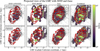 |
Fig. 1 Comparison of the density maps between the different LMC clean samples. Top: LMC complete sample. Bottom: LMC optimal sample. From left to right, APOGEE, BOSS, Gaia, and Combined sample. We display bins containing three or more stars; otherwise, we display individual stars as a scatter plot. The brighter colours correspond to the higher density zones. A red line splitting the overdensities (LMC bar and spiral arm) from the underdensities is plotted. All maps are shown in the LMC in-plane (x′, y′) Cartesian coordinate system. To mimic how the LMC is seen in the sky, the plotted data has both axes inverted. |
2.1 SDSS sample
We choose stars in the LMC sky area from the SDSS-V’s MWM dataset (BOSS and APOGEE) and the SDSS-IV survey (APOGEE DR17) that have line-of-sight velocity information. We do so by restricting our selection to a region of 15∘ radius around the LMC’s photometric centre, defined as (αc, δc) = (81.28∘, −69.78∘) by van der Marel (2001).
With this initial cut, we obtained 55 845, 22 374, 11 328 stars for the BOSS MWM, APOGEE MWM, and APOGEE DR17 surveys, respectively. The APOGEE DR17 and MWM datasets were combined into a single sample called APOGEE with a total of 33 702 stars. We refer to the BOSS MWM sample as BOSS for simplicity.
Because of the selection function of the BOSS and APOGEE surveys, stars in these samples are not uniformly distributed in the sky, which makes the footprint – composed of hexagonal patches – highly visible (see, for example, Fig. 1). The reader may notice that this SDSS sample, with a total of 89 547 (APOGEE + BOSS) stars, contains both LMC and MW stars. The following section (Sect. 2.2) discusses how we obtain LMC clean samples, after removing the MW foreground contamination. We also note that, since we have enough coverage of the LMC’s disc (Fig. 1), and we primarily concern ourselves with modelling the moments of distributions (means and medians), our results are unaffected by the uneven footprint imposed by the selection function.
2.2 Gaia LMC clean samples
To remove foreground MW star contamination from our Gaia LMC base sample, we follow the neural-network (NN) technique from Jiménez-Arranz et al. (2023b) and Jiménez-Arranz et al. (2023a), as a parallax based distance distinction has been shown to not be a reliable method due to their high uncertainties (e.g. Gaia Collaboration 2021b; Lindegren et al. 2021). This methodology enables the classification of three different samples of candidate LMC stars with different degrees of completeness and purity. Since in this work we aim to verify the robustness of our results with this trade-off between completeness and purity, we employ both the NN complete and NN optimal LMC clean samples from Jiménez-Arranz et al. (2023b). In a similar fashion to the SDSS samples, the Gaia LMC clean samples are restricted to a region of 15∘ radius around the LMC centre, defined as (αc, δc) = (81.28∘, −69.78∘) by van der Marel (2001).
The NN complete sample corresponds to the sample that prioritises not missing LMC stars at the price of a possible increased MW contamination. It contains 12 116 762 stars. Conversely, the NN optimal sample differs in the trade-off between completeness and purity, with less MW contamination than the NN complete sample but losing some LMC stars. It contains 9 810 031 stars. Both samples are dominated by older stellar populations (see, e.g. Fig. 3 from Gaia Collaboration 2021b). We stress that, since the purity-completeness trade-off is a decision that will define the properties of the resulting sample and therefore can have an effect on the results obtained from it, we kept both samples for this study.
A sub-sample of bright stars (G ≲ 17.65, De Angeli et al. 2023) of the LMC NN complete and NN optimal samples have Gaia DR3 line-of-sight velocity information. This is obtained with the Radial Velocity Spectrometer (RVS, e.g. Katz et al. 2004; Cropper et al. 2018; Katz et al. 2023). The instrument is a near-infrared (845−872 nm), medium-resolution (R ∼ 11 500), integral-field spectrograph dispersing all the light entering the field of view. We refer to these sub-samples with Gaia RVS line-of-sight velocities as the corresponding Vlos sub-samples. The LMC complete and optimal Vlos sub-samples contain 30 749 and 22 686 stars, respectively.
As illustrated in Fig. 9 of Jiménez-Arranz et al. (2023b) and in Fig. 2 of this work, if we assume that the MW stars have line-of-sight velocities of less than 125 km s−1, then the MW contamination for the complete (optimal) Vlos sub-samples is approximately ∼5% (∼0%). Since this subset only contains stars at the bright end (G ≲ 16) of the Gaia sample, we can observe that it maximises the performance of the classifier.
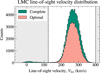 |
Fig. 2 Distribution of the line-of-sight velocities of the LMC Combined complete (green) and optimal (salmon) sample. The vertical black dashed lines delimit the area of the LMC stars that are kept, namely, 125 km/s < Vlos < 400 km/s, to reduce MW foreground contamination. |
2.3 Cross-matching the SDSS data with the Gaia LMC clean samples
We cross-match the SDSS sample obtained in this work with the LMC/MW classifier created by Jiménez-Arranz et al. (2023b) in order to remove any MW contaminants. Through this crossmatch between surveys, we are also able to provide to the SDSS sample the necessary astrometric and photometric data for this study. As previously mentioned, we retain both the LMC NN complete and NN optimal samples for this study because the purity-completeness trade-off determines the characteristics of the final sample and may therefore impact the result. Hereafter, we remove “NN” from the LMC complete and optimal sample for the purpose of simplicity.
The cross-match between the SDSS and the Gaia sample is done using Gaia’s DR3 source_id. Furthermore, every star in the APOGEE MWM sample has a match with the previous Gaia Data Release (Gaia DR2). In general, the only safe way to compare source records between different data releases is to check the records of proximal sources in the same small part of the sky, since it is not guaranteed that the same astronomical source will always have the same source identifier in different Gaia Data Release. The gaiadr3.dr2_neighbourhood table of Gaia DR3 offers a precomputed crossmatch of these sources that accounts for the proper motions available in DR3. There may be none, one, or (rarely) many potential DR2 counterparts in the vicinity of a particular DR3 source. This occasional source confusion is an inevitable consequence of the merging, splitting and deletion of identifiers introduced in previous releases during the DR3 processing and results in no guaranteed one-to-one correspondence in source identifiers between the releases. In this work, if a Gaia DR3 star has multiple potential counterparts in DR2, we retain the closest match (based on sky position) for the cross-match between the APOGEE MWM and Gaia sample.
In order to account for the different SDSS and Gaia LMC clean samples, we define the following eight samples with full velocity information (both proper motion and line-of-sight velocities) for the remainder of the paper:
Sample 1 (2): APOGEE complete (optimal) sample;
Sample 3 (4): BOSS complete (optimal) sample;
Sample 5 (6): Gaia complete (optimal) sample;
Sample 7 (8): Combined complete (optimal) sample.
The characteristic uncertainty of each dataset in the line-of-sight velocity is ∼1 km s−1, ∼5 km s−1, and ∼3 km s−1 for APOGEE, BOSS, and Gaia, respectively. Moreover, the stars in the Combined sample have line-of-sight velocities that are arranged to prioritise the source of the data in the following order; use the APOGEE line-of-sight velocity if an APOGEE observation is available. If not, consider the BOSS line-of-sight measurement. Finally, use the Gaia line-of-sight velocity if there is no SDSS (APOGEE or BOSS) line-of-sight measurement for this star. We are using line-of-sight velocities from BOSS before Gaia to reduce the effect of using different datasets in the inner and outer regions of the LMC; moreover, the signal-to-noise distribution of BOSS targets is higher than that of Gaia. Furthermore, we verified that the outcomes of this work are robust regardless of whether BOSS or Gaia is prioritised first. Finally, this approach prioritises the new SDSS dataset. Therefore, despite variations in resolution and signal-to-noise ratio, the line-of-sight velocity measurements from the various surveys are in good agreement and do not bias the results and conclusions of this work. Since some stars have line-of-sight velocity measurements from multiple surveys, the number of stars in the Combined sample is less than the sum of the three samples (APOGEE, BOSS, and Gaia).
Number of sources for the different LMC clean samples.
Lastly, in order to reduce MW foreground contamination in our samples, we apply the following cut, 125 km/s < Vlos < 400 km/s, to select stars with line-of-sight velocities that are compatible with the LMC’s systemic motion. The distribution of the line-of-sight velocities of the LMC Combined complete and optimal sample is displayed in Fig. 2. Table 1 summarises the number of sources for the different LMC clean samples.
2.4 De-projection of coordinates into the LMC’s disc plane
Since the main goal of this work is to look at the vertical internal (off-plane) kinematics of the LMC, we use the coordinate transformation developed and used in van der Marel (2001); van der Marel et al. (2002); Jiménez-Arranz et al. (2023b) to deproject all coordinates into the LMC’s disc reference frame. We assume that all stars lie in the z′ = 0 plane, and use the inclination, position angle, and position of the LMC centre given in Jiménez-Arranz et al. (2023b). Nonetheless, we re-derive the systemic motion for both proper motion and line-of-sight velocity by taking into account the median velocity value of a 0.5∘ inner circle in the LMC’s disc, since asymmetries in the LMC are well-known (e.g. Olsen & Salyk 2002; Niederhofer et al. 2022; Cullinane et al. 2022a,b; Jiménez-Arranz et al. 2023b, 2024a; Kacharov et al. 2024; Dhanush et al. 2024; Rathore et al. 2025), as are the varying kinematics of different populations (see, for example, Table 1 of Gaia Collaboration 2021b). Therefore, it is possible that the global rotation model fitted in Gaia Collaboration (2021b) to one sample of stars would yield a slightly different result from the actual velocities of stars in the vicinity of the adopted centre of a different sample, such as the one used in this work (see Sect. 3 for the updated values for the systemic motions). The LMC centre matches its photometric centre (van der Marel 2001) and is the same as that used in Gaia Collaboration (2018b, 2021b).
Like any extra-galactic study of the kinematics of discs, we must make use of the infinitely thin disc approximation (z′ = 0). This is because, unlike stars in the MW (Gaia Collaboration 2023a), or a few variable stars in the LMC (Cusano et al. 2021; Ripepi et al. 2022), the 3D position space of stars in the LMC is not available. Our methods characterise the mid-plane (namely, the vertical symmetry plane) of the stellar distribution. This midplane is a thin plane, even when the stellar distribution itself is not thin. The thickness of the plane only adds uncertainty to the transformation of proper motions to in-plane velocities in km s−1. Once we have identified the correct viewing angles, the distribution of stars around the plane is symmetric. Thus, this primarily adds additional scatter to velocity maps (such as Fig. 4), and not a bias. In addition, any errors we could be introducing are small. Since the LMC disc thickness (not greater than 1 kpc, see Ripepi et al. 2022, for example) is small in comparison to the LMC mean distance (≈50 kpc, Pietrzyński et al. 2019), the implications on the kinematics are minor.
Figure 1 shows the in-plane density distributions for the different LMC clean samples. To visualise the de-projected positions and velocities in the LMC in-plane (x′, y′) Cartesian coordinate system for each star, we use the coordinate transformation described in van der Marel (2001), van der Marel et al. (2002) and Jiménez-Arranz et al. (2023b). In the top (bottom) panels, we show the LMC complete (optimal) APOGEE, BOSS, Gaia, and Combined sample, from left to right. A general characteristic across samples is that the LMC optimal sample does not cover the outer regions as much as the LMC complete sample. This is expected since, as we get more complete, we can anticipate more MW contamination, which is more likely to happen on the outskirts of the LMC, where the classifier might encounter problems. A red line splitting the overdensities (LMC bar and spiral arm) from the underdensities is plotted for reference – for more details see Sect 4.2 of Jiménez-Arranz et al. (2023b).
Stars in the inner region of the LMC, near the galactic bar, are observed in the APOGEE samples, while stars in the arm and the inter-arm region are observed by BOSS. As mentioned in Sect. 2.1, both samples show the footprint of the surveys’ selection function, being more patchy for the BOSS sample (showing hexagonal shapes)1. One may observe that certain hexagonal patches, such as those centred in (x′, y′) = (1, 3) kpc and (1, −5) kpc, exhibit an exceptionally high density in the LMC disc region throughout the complete BOSS sample. This is due to the fact that some LMC fields have high priority Transiting Exoplanet Survey Satellite (TESS, Ricker et al. 2015) targets that need more epochs. Some of these high density patches in the BOSS samples disappear in the LMC optimal sample, as (x′, y′) = (1, −5) kpc, showing that they were likely mostly remnants of the MW contamination, whereas others, e.g. at (x′, y′) = (1, 3) kpc, remain. The Gaia samples are relatively uniform, showing a decrease in density with radius, with a densely populated bar region and a sparsely populated arm area. After merging all these three samples (APOGEE, BOSS and Gaia), we obtain the LMC Combined samples, with a fair coverage of the whole LMC disc.
Finally, we advise the reader that for most figures and analyses in this paper the two samples (LMC complete and optimal) yield qualitatively similar results, and we therefore generally show results only for the optimal sample for the figures comparing the two samples, see Appendix B. However, in cases where the two samples yield answers for a quantity of interest that differs by more than the statistical uncertainties, we discuss both results using the distinct LMC samples. The difference between the results for the two samples can then be used to assess any systematic uncertainties.
2.5 Selecting stars at different evolutionary phases
Based on the unique properties of the various spectroscopic instruments, different evolutionary phases are observed by each survey. To perform the LMC in-plane kinematic analysis for different stellar populations, we choose the target evolutionary phases by defining cut-outs with polygonal shape in the colour-magnitude diagram (CMD), as in Gaia Collaboration (2021b) – see their Sect. 2.3 and Fig. 2. Even though it is not corrected from reddening, this rather crude selection can be used as an age-selected proxy to some extent. We define the stellar evolution areas as exclusive. Thus, they do not overlap. Based on the definition in Gaia Collaboration (2021b), we consider the following evolutionary phases:
Young 1: very young main sequence (ages < 50 Myr);
Young 2: young main sequence (50 < age < 400 Myr);
Young 3: intermediate-age main-sequence population (mixed ages reaching up 1–2 Gyr);
RGB: red giant branch;
AGB: asymptotic giant branch (including long-period variables);
RRL: RR-Lyrae region of the diagram;
BL: blue loop (including classical Cepheids);
RC: red clump.
The top panel of Fig. 3 shows the Gaia CMD of the LMC optimal sample with the areas of the different evolutionary phases. The second row shows the CMD of the different surveys for the LMC optimal sample. We display, from left to right, the LMC optimal APOGEE, BOSS, Gaia, and Combined sample. These panels show that the majority of the stars that APOGEE observes are in the very bright evolutionary phases, such as AGB and BL stars. While some AGB, BL, and Young stars are observed, the bulk of RGB stars are found in the BOSS survey. It is noteworthy that while the majority of LMC targets in SDSS-IV were RGB, SDSS-V is currently observing AGB stars. Gaia provides line-of-sight velocities for AGB and BL stars. Considering this, we can divide the Combined sample into distinct evolutionary phases that have ample coverage from APOGEE, BOSS, and Gaia data. We considered the Young (hereafter, the joined Young 1, Young 2, and Young 3 samples), RGB, AGB, and BL Combined samples. The number of sources for each evolutionary phase of the LMC Combined sample and the contribution from each sample (APOGEE, BOSS and Gaia) is summarised in Table 2.
Number of sources for each evolutionary phase of the LMC Combined sample with sufficient statistics.
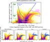 |
Fig. 3 Top panel: colour-magnitude diagram of the LMC optimal sample (9 810 031 stars) with the areas of the different evolutionary phases (as defined by the polygons given in Gaia Collaboration 2021b). Second row: Comparison of the CMD between the different surveys for the LMC optimal sample. From left to right: APOGEE, BOSS, Gaia, and Combined sample. In each sample, the foreground image represents the relative density of stars with line-of-sight velocity. Higher densities are highlighted by lighter (greener) colours, while lower densities are shown by darker (bluer) colours. The background of the bottom panel displays the CMD for the optimal LMC sample, which consists of 9 810 031 stars. The colours represent the relative stellar density, with darker colours indicating higher densities. |
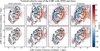 |
Fig. 4 Comparison of the median vertical velocity maps between the different LMC clean samples. Top: LMC complete sample. Bottom: LMC optimal sample. From left to right, APOGEE, BOSS, Gaia, and Combined sample. We display bins containing three or more stars; otherwise, we display individual stars as a scatter plot. A black line splitting the overdensities (LMC bar and spiral arm) from the underdensities is plotted for reference. All maps are shown in the LMC in-plane (x′, y′) Cartesian coordinate system. To mimic how the LMC is seen in the sky, the plotted data has both axes inverted. |
3 Vertical velocity maps and profiles
Thanks to the larger sample of line-of-sight velocities provided by SDSS-IV/V, we aim to provide a more extensive map of the LMC vertical (off-plane) velocity vz′ than the one given in Jiménez-Arranz et al. (2023b) using Gaia DR3 data – see their Fig. 17. The coordinates transformations to deproject the LMC are summarised in Sect. 2.4. We advise the reader to consult van der Marel (2001), van der Marel et al. (2002) and Jiménez-Arranz et al. (2023b) for additional information regarding the coordinate transformation and their underlying assumptions.
We use the inclination, position angle, and position of the LMC centre derived in Gaia Collaboration (2021b) and used in Jiménez-Arranz et al. (2023b). Nonetheless, we re-derive the systemic motion for both proper motion (μα*,0, μδ,0) and line-of-sight velocity (μz,0) for the LMC Combined complete and optimal sample by computing the median velocity value within a 0.5∘ with respect to the LMC centre. The LMC Combined complete sample recovers a systemic motion of: μα*,0 = 1.914 ± 0.003 mas yr−1; μδ,0 = 0.384 ± 0.002 mas yr−1, and; μz,0 = −1.113 ± 0.001 mas yr−1. We adopt the same systemic motion for both LMC Combined complete and optimal since the variations are negligible – differences lie within the uncertainties. Uncertainties are derived as MAD/ , where ‘MAD’ stands for median absolute deviation. Table 3 compares the systemic motions used in this paper with those used in Gaia Collaboration (2021b).
3.1 LMC clean samples
Figure 4 shows the median vertical velocity maps between the different LMC clean samples. The vertical velocity maps have second order differences between the LMC complete and optimal samples. The Combined samples exhibit a trend that is consistent with that reported by the Gaia sample (Jiménez-Arranz et al. 2023b). A bimodal trend can be seen in the vertical velocity map, with half of the galaxy (x′ < 0) moving upwards and the other half (x′ > 0) moving downward. Additionally, a gradient of increasing (median) vertical velocities from the inner to the outer disc appears to be positive (in absolute value). This could be associated with either: an overestimation of the disc inclination angle (e.g. Jiménez-Arranz et al. 2023b); the presence of a galactic warp (e.g. Choi et al. 2018; Saroon & Subramanian 2022); or due to the fact that the LMC is not in dynamical equilibrium (e.g. Belokurov et al. 2019; Choi et al. 2022; Jiménez-Arranz et al. 2024a,b, see Sect. 4). Additionally, stars at the end of the bar with x′ > 0 appear to be moving clearly in a negative direction, which may indicate that the bar is inclined with respect to the galactic plane (e.g. Besla et al. 2012; Choi et al. 2018).
Comparison of the LMC systemic motion between this work and Gaia Collaboration (2021b).
We detect a ‘blob’ of stars with median negative vertical velocities2 of around ∼−15 km s−1 in the centre of the inner arm, at about (x′, y′) = (−1, −3) kpc. This region corresponds to the supershell LMC 4 (e.g. Vallenari et al. 2003; Book et al. 2008; Fujii et al. 2014; Ou et al. 2024), a structure of ionised material with size ≈ 1 kpc (for a review read Tenorio-Tagle & Bodenheimer 1988; Dawson et al. 2013a); this is the largest bubble-like structure in the LMC. When projection effects are taken into account, the supershell LMC 4 is almost perfectly circular with a diameter of ∼1400 pc, and is expanding with a velocity of ∼36 km s−1 (e.g. Dopita et al. 1985; Ou et al. 2024). Star formation appears to have started approximately ∼15 Myr ago. We believe it is the first time that the supershell LMC 4 is observed in the (vertical) kinematics space of individual LMC stars. We show later in Sect. 3.2 how this kinematic feature is exclusive to the young stars. Figure 5 is a representation of supershell LMC 4 – in the LMC in-plane (x′, y′) Cartesian coordinate system – using astrometric and photometric data from Gaia DR3.
3.2 Dependence on stellar evolutionary phases
With the various evolutionary phases presented in Sect. 2.5, we are able to construct the vertical velocity maps for the LMC Combined sample. In this way, the kinematic differences between different stellar tracers of the LMC can be analysed independently.
Figure 6 shows the median vertical velocity maps between the different evolutionary phases of the LMC Combined optimal sample. In the top (bottom) panels, we show the LMC complete (optimal) Young, BL, AGB, and RGB samples, from left to right. Among all evolutionary phases, we observe that the Young sample is the least represented, due to target selection reasons. This population primarily follows the edges of the LMC bar, except for a few stars towards the east (i.e. the right side of Fig. 6), towards the position of the SMC. The supershell LMC 4 that was observed in Fig. 4 and discussed in Sect. 3.1 is exactly traced by the Young population in the inner arm of the LMC. It shows its characteristic negative vertical velocity (|vz′ | ∼−20 km s−1). The BL stars trace the LMC bar, the LMC’s periphery, and the inner spiral arm, reiterating the kinematic imprint of the supershell LMC 4. For the BL stars, the area of the arm that is attached to the bar appears to be moving at a null vertical velocity, which is different from the positive vertical velocities seen in the older (AGB) stellar sample.
Including the bar and spiral arm(s), the AGB stars trace the entire LMC disc. The lack of the blue (negative vertical velocities) “blob” produced by the supershell LMC 4 is the main significant difference with the LMC Combined sample. Finally, the RGB stars, that are primarily observed by BOSS, appear unevenly distributed across the LMC disc due to the survey’s footprint. This population also traces the inner part of the LMC bar. Due to the low number statistics for RGB stars in this region, we are unable to assess their vertical velocity profile.
After inspecting the position of stars in the supershell LMC 4 in the CMD, we have found that the majority of this sample is comprised by bright BL stars, followed by Young 1 stars. However, there is also a co-spatial population of AGB stars with non-LMC 4 supershell such as v′z velocities (i.e. centred around v′z = 0 km s−1, instead of v′z = −20 km s−1).
In a similar vein, we use the MAD to compute the dispersion of the vertical velocity of the different evolutionary phases of the LMC Combined sample, shown in Fig. 7. The arrangement of the subplots is identical to that of Fig. 6. As expected, we find that the Young and BL samples, which comprise the younger evolutionary phases, exhibit a smaller velocity dispersion (of the order of ∼5 km s−1) due to them being kinematically colder in comparison to the AGB and RGB samples, which comprise the older evolutionary phases. The AGB has a median vertical velocity dispersion around ∼12−15 km s−1, whereas median dispersion of the RGB sample is above ≳20 km s−1. In the region of the supershell LMC 4, the vertical velocity dispersion is smaller for the Young and BL sample than for the AGB sample.
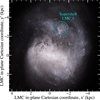 |
Fig. 5 Representation of the LMC using astrometric and photometric information from the Gaia DR3. This view is not a photograph since it has been compiled by mapping the total amount of radiation detected by Gaia in each pixel, combined with measurements of the radiation taken through different filters on the spacecraft to generate colour information. The MW contamination has been removed because the NN Complete sample of Jiménez-Arranz et al. (2023b) has been used. All types of stellar populations are shown. The cyan ring is centred on the supershell LMC 4 (α = 5h32m, −66∘40′, Book et al. 2008), with a diameter of 1400 pc (Dopita et al. 1985; Ou et al. 2024). The representation is done in the LMC in-plane (x′, y′) Cartesian coordinate system, as in Fig. 4. This represents a face-on view that is corrected for the viewing inclination. |
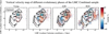 |
Fig. 6 Comparison of the median vertical velocity maps between the different evolutionary phases (see Fig. 3) of the LMC Combined optimal sample. From left to right, Young, BL, AGB, and RGB samples – following a rough sequence in age. We display bins containing three or more stars; otherwise, we display individual stars as a scatter plot. A black line splitting the overdensities (LMC bar and spiral arm) from the underdensities is plotted. The cyan ring is centred on the supershell LMC 4 (α = 5h32m, −66∘40′, Book et al. 2008), with a diameter of 1400 pc (Dopita et al. 1985; Ou et al. 2024). All maps are shown in the LMC in-plane (x′, y′) Cartesian coordinate system. To mimic how the LMC is seen in the sky, the plotted data has both axes inverted. |
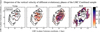 |
Fig. 7 Same as Fig. 6 but for the vertical velocity dispersion – given by the MAD. We only display bins containing three or more stars. Larger vertical velocity dispersion corresponds to darker colours. |
3.3 Azimuthal analysis
In Fig. 8, we present the one-dimensional vertical velocity profiles as a function of azimuth, ϕ, defined in the LMC in-plane (x′, y′) coordinate system. To do so, we bin the data in 16 angular wedges, each of 22.5∘ in width (see the schema in the top panel of Fig. 8). From top to bottom, we show the LMC optimal Combined, BL, AGB, and RGB samples. The Young sample is not shown due to low number statistics.
For the Combined sample we note that, near the LMC centre (R′ ≲ 1.75 kpc), the azimuthal wedges along the line-of-nodes (x′ ∼ 0), namely, ϕ ∼ 0∘ and ϕ ∼ 180∘ with green lines, exhibit a distinct trend for the vertical velocity vz′. The vertical velocity shows a linear increase (decrease) as function of the LMC galactocentric radial distance in the ϕ ∼ 0∘ (ϕ ∼ 180∘) wedge, as can be seen in the right panels of Fig. 4. On the other hand, the azimuthal wedges perpendicular to the line-of-nodes (y′ ∼ 0), namely, ϕ ∼ 90∘ and ϕ ∼ −90∘ with red and blue lines, show a flatter behaviour for all radius. The curves corresponding to the various wedges flatten at larger radii (R′ ≳ 4 kpc), with similar dispersion for both the LMC Combined complete and optimal samples.
If we look at the different stellar populations, we are unable to determine whether the RGB stars exhibit the observed linear trend of vertical velocity with respect to the galactocentric radius due to the limited coverage of RGB stars in the LMC centre. Nonetheless, it exhibits flattened curves with azimuth, and follows the same trend in the LMC outskirts as the LMC Combined sample. The situation is reversed for the AGB and BL stars, where the inner LMC region has better coverage than the outer regions. This allows us to see the same linear relationship near the centre of the LMC. In the following section, we provide a more thorough analysis of this kinematical behaviour.
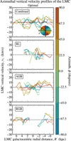 |
Fig. 8 Comparison of the azimuthal vertical velocity profiles between the LMC optimal Combined sample and its different evolutionary phases. From top to bottom, Combined, BL, AGB, and RGB samples. Because of its low statistical representation, the Young sample is not displayed. Only radial bins with more than 25 sources are plotted. Each colour corresponds to a different azimuth ϕ defined in the LMC in-plane (x′, y′) Cartesian coordinate system – see schema in the top right panel. The vertical velocity uncertainty of each bin, determined by the MAD/ |

4 Interpretation of the LMC velocity maps
In the previous section, we showed that there is a dipole in the vertical velocity plane of the LMC disc (Figs. 4 and 6). This may be due to different factors. In Sect. 4.1, we examine whether this vertical velocity signature may be due to a time variability in the LMC disc’s viewing angles. In Sect. 4.2, we examine whether this kinematic feature could be the result of using an incorrect LMC disc plane, given by the inclination, i, and line-of-nodes position angle, Ω. In Sect. 4.3, we examine whether we could be observing the imprint of a warp within the LMC disc. Finally, in Sect. 4.5, we discuss how the choice of the LMC centre affects the robustness of our findings.
4.1 The rate of change in the LMC’s disc viewing angles
A dipole in the LMC vertical velocity maps could be explained by time variability in the LMC disc viewing angles, namely, that is, a non-zero rate of change di/dt for the inclination and dΩ/dt for the line-of-nodes position angle dΩ/dt. This would result in a solid body rotation of the LMC disc.
The LMC rate of inclination change, di/dt, was first fitted by van der Marel et al. (2002) using line-of-sight measurements of 1041 carbon stars (see their Eq. 41). With new line-of-sight observations for both gas and stellar populations, subsequent works have attempted the same endeavour in a similar fashion (e.g. Olsen & Massey 2007; Olsen et al. 2011). However, the line-of-sight velocity field does not provide any information on time variations in the position angle of the line of nodes, dΩ/dt. This makes it impossible to compute the past or future variation in the LMC symmetry axis orientation in an inertial frame tied to the MW.
The method used in van der Marel et al. (2002) to estimate di/dt was tailored to a case without astrometric information, and assuming circular orbits to make up for the absence of full 3D velocity information. Now, thanks to the spectro-astrometric data provided by the Gaia and SDSS-IV/V missions (see Sect. 2 for details), we have access to the vertical velocities for the LMC disc (Jiménez-Arranz et al. 2023b, and this work). Under the assumption that these robustly describe the true vertical velocities across the LMC disc plane, this allows us to estimate both the rate of change in the LMC’s disc inclination di/dt and the line-of-nodes angle dΩ/dt using a more direct method.
Equation (6) of van der Marel & Cioni (2001) gives the LMC off-plane coordinate z′ as a linear sum of the LMC orthographic coordinates (x, y, z) multiplied by trigonometric terms involving the inclination i and the line-of-nodes position angle Ω. Then, we can take the time derivative of this equation at fixed (x, y, z). This yields the LMC vertical velocity vz′ as a linear sum of (x, y, z) multiplied by linear combinations of di/dt and dΩ/dt that contain trigonometric terms involving the LMC viewing angles. Equation (4) of van der Marel & Cioni (2001) paper gives each of the LMC orthographic coordinates (x, y, z) as a linear sum of the LMC deprojected coordinates (x′, y′, z′) multiplied by trigonometric terms involving the LMC viewing angles. If we substitute these equations for (x, y, z) in the result of above, it yields the LMC vertical velocity vz′ as a linear sum of (x′, y′, z′) multiplied by linear combinations of di/dt and dΩ/dt that involve trigonometric terms involving the LMC viewing angles. In this linear sum, most of the terms cancel and drop out, leaving
 (1)
(1)
The LMC vertical velocity maps vz′ from the previous section (see Fig. 4) can be modelled as a disc with solid body rotation defined by di/dt and dΩ/dt, which we can be fitted using this equation. For the LMC Combined complete sample, we thus obtained the rate of change in the LMC’s disc viewing angles to be
 (2)
(2)
For the LMC Combined optimal sample, we obtained:
 (3)
(3)
The statistical errors are computed by bootstrapping with replacement within the measured uncertainties of 1000 pseudo-samples. Figure 9 compares the median vertical velocity maps between the different LMC Combined samples, the disc model with a solid body rotation, and the residuals. Top (bottom) panels show the LMC Combined complete (optimal) sample. From left to right we show the vertical velocity maps for the data (same as right panels of Fig. 4), the disc model with a solid body rotation, and the residuals (data minus model). We can observe in the residuals maps that the inclusion of di/dt and dΩ/dt helps reduce the variance in the vz′ maps in the inner regions. However, the residual vertical velocity maps (right panels) clearly retain significant residual structure that cannot be attributed solely to non-zero values of di/dt and dΩ/dt. This implies that (a) other effects may be responsible for (or contributing to) the structure in the vz′ maps (see Sects. 4.2 and 4.3); and/or (b) the random uncertainties by themselves are not a good measure of the true uncertainties in di/dt and dΩ/dt.
The systematic uncertainties in our new determinations of di/dt and dΩ/dt are at least as large as the difference between the results for the two samples. Our determinations of di/dt and dΩ/dt are in fact entirely meaningless, if other effects are the main cause of the non-zero values and dipole in the vz′ vertical velocity maps, which we explore in subsequent sections. We discuss the results obtained in this section and compare our estimations of di/dt and dΩ/dt with other values found in the literature in Sect. 5.
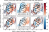 |
Fig. 9 Comparison of the median vertical velocity maps between the different LMC Combined samples and the disc model with a solid body rotation. Top: LMC complete sample. Bottom: LMC optimal sample. From left to right, Data (Combined sample), model and residuals. We only display bins containing three or more stars. A black line splitting the overdensities (LMC bar and spiral arm) from the underdensities is plotted. All maps are shown in the LMC in-plane (x′, y′) Cartesian coordinate system. To mimic how the LMC is seen in the sky, the plotted data has both axes inverted. |
4.2 Assuming an incorrect disc plane
Another possible explanation of the dipole present in the LMC vertical velocity maps could be that such measurements are nonphysical. This feature may be produced by assuming an incorrect LMC disc plane, defined by the inclination, i, and the line-of-nodes position angle, Ω, which is the position angle of the receding node, measured from y towards x, that is, from north towards east3.
In the previous sections, we assumed the LMC disc plane fitted by Gaia Collaboration (2021b), with i = 34∘ and Ω = 310∘, as the true LMC disc plane. In this work, the authors fitted the LMC proper motion as a flat rotating disc with average vR = 0 and vϕ = vϕ(R), where vR and vϕ are galactocentric in-plane polar velocities, to determine the LMC disc plane; namely, assuming circular velocities. However, it is known that the LMC is intrinsically elongated (e.g. van der Marel 2001). Therefore, the true LMC disc plane obtained under this assumption may be biased. Moreover, to add more complexity to this problem, in the literature we can find a range of estimates of the LMC inclination and the line-of-nodes position angle provided by different methods (e.g. van der Marel & Kallivayalil 2014; Haschke et al. 2012; Ripepi et al. 2022; Kacharov et al. 2024), with differences that can be as large as 10∘. Thus, these two crucial assumed quantities are by no means a well constrained measurement.
In this section, to determine whether the bimodal trend seen in the LMC vertical velocity maps could be the result of an incorrect disc plane assumption, we fit instead the LMC disc plane by minimising the RMS vertical velocity, vz′, across the disc of the LMC. To do so, the statistic that we minimised to find the best fitting values of the inclination and the line-of-nodes position angle is a chi-squared that can be explicitly written as follows:
 (4)
(4)
We remind the reader that the detailed relation vz′ = vz′(i, Ω) can be found in van der Marel (2001), van der Marel et al. (2002) and Jiménez-Arranz et al. (2023b). We use the SciPy (Virtanen et al. 2020) implementation of the Nelder-Mead simplex algorithm (Nelder & Mead 1965) to minimise χ2.
For the LMC Combined optimal (complete) sample, we recover a disc plane with inclination i = 23.6∘ ± 0.1∘ (i = 20.0∘ ± 0.1∘) and the line-of-nodes position angle Ω = 326.9∘ ± 0.3∘ (Ω = 330.0∘ ± 0.2∘). The statistical errors are computed via bootstrapping with replacement of 25 pseudo-samples. Moreover, to ensure the robustness of the optimisation, each pseudo-sample run started with a different initial guess of (i, Ω). It is worth mentioning that both the LMC Combined complete and optimal samples provide a robust estimation of (i, Ω) with a difference of ∼3∘, which can be considered as the systematic error. Finally, we observe that, in comparison to the values obtained by the authors of Gaia Collaboration (2021b), namely i = 34∘ and Ω = 310∘, the LMC disc plane inclination i and the line-of-nodes position angle Ω that we recover for the LMC Combined optimal (complete) sample differ by δi ∼ 10∘ (δi ∼ 14∘) and δ Ω ∼17∘ (δ Ω ∼20∘). When compared to the LMC viewing angles of Kacharov et al. (2024), also based on 3D kinematics, their estimate of the inclination (i = 25.5∘ ± 0.2∘) is similar to ours, while their estimate for the line-of-nodes position angle (Ω = 304∘ ± 0.4∘) is not. We address the potential reasons for these discrepancies in Sect. 5.
The left panels of Figure 10 show the median vertical velocity maps for the LMC Combined complete (top) and optimal (bottom) samples, in a similar fashion to right panels of Fig. 4, but for the best LMC disc plane fitted by minimising the RMS vertical velocity. When comparing the kinematic maps of the assumed (Gaia Collaboration 2021b) and fitted values (this work) of i and Ω (i.e. Figs. 4 and 10), we observe the following features: 1) the LMC bar major axis becomes less aligned with the line-of-nodes due to the change of plane – we note there is no physical reason that the two should be aligned; 2), the LMC bar’s bimodal vertical velocity trend vanishes, leaving behind a nearly null median vertical velocity; 3) there is a sign change in the disc’s vertical velocity bimodal trend. Compared to the positive values in Fig. 4, the part of the spiral arm attached to the bar now shows a negative vertical velocity. Lastly, and in connection with the previous point, 4) the supershell LMC 4 continues to stand out from the background, albeit not as much as with the LMC disc plane fitted in Gaia Collaboration (2021b).
While the newly determined disc plane (by definition) provides a lower RMS vertical velocity than the one determined by Gaia Collaboration (2021b), the median maps in the left panels of Fig. 10 continue to show significant residual structure. This implies that the underlying assumption of this section –that the structure observed in the vertical velocity maps is solely due to incorrect constant viewing angles– is incomplete. Something else must be responsible for the majority of the vertical velocity structure, which we examine in the next section.
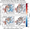 |
Fig. 10 Comparison of the median vertical velocity maps for the different LMC Combined samples (top: complete sample; bottom: optimal sample) obtained with different assumptions about the LMC disc plane. Left: Results for the best-fitting flat plane, obtained by minimising the RMS vertical velocity vz′, with viewing angles listed in the panels. Right: Results for the best best-fitting warped plane, with viewing angles shown in Fig. 12. When comparing the top and bottom panels, the reader should note that the overdensity lines differ slightly because each LMC sample uses a different disc plane. |
4.3 Warp in the LMC disc
Since the LMC was previously found to contain a warp (e.g. van der Marel & Cioni 2001; Olsen & Salyk 2002; Nikolaev et al. 2004; Choi et al. 2018; Ripepi et al. 2022), it is important to assess the validity of the assumption in Sect. 4.2 that the disc plane can be characterised by constant values of (i, Ω).
First, for distinct annular rings in the (x′, y′) plane – defined by the inclination angle, i, and the line-of-nodes position angle, Ω, of Gaia Collaboration (2021b), Sect. 3 –, we repeat the best fit disc plane minimisation of Sect. 4.2 to quantify the change of (i, Ω) as function of the LMC galactocentric radial position R′. Figure 11 (left panels) displays the variation in the fitted LMC disc plane as function of the LMC galactocentric radius, R′. In the top (bottom) panel, we show the derived inclination i (the line-of-nodes position angle Ω) for both the LMC Combined complete and optimal samples in green and salmon colours, respectively. The horizontal dashed lines show the “global” fit found for each sample in Sect. 4.2. In the top panel, we observe that in both samples the inclination is low (i ∼ 10∘) at the inner regions (R′ ∼ 0 kpc) and grows up to values of i ∼ 25∘ for the outer disc (R′ ≳ 3.5 kpc). The LMC Combined complete and optimal samples have an almost constant off-set of approximately δi ∼ 2∘− 3∘, with the LMC Combined optimal sample having a systematically larger inclination. The bottom panel illustrates that the line-of-nodes position angle in both samples is high (Ω ∼ 335∘− 350∘) at inner regions (R′ ∼ 0 kpc), decreases to values of Ω ∼ 320∘− 325∘ at approximately R′ ∼ 2.5 kpc, and then increases once more to values of Ω ∼ 335∘ in the outer disc (R′ ≳ 3.5 kpc). For nearly all LMC galactocentric radii, there is an almost constant off-set of approximately δ Ω ∼ 5∘ between the LMC Combined complete and optimal sample, with the LMC Combined complete sample displaying a larger line-ofnodes. We highlight with a grey shaded area the LMC bar region, R′bar = 2.3 kpc, found by Jiménez-Arranz et al. (2023b).
Second, we can also quantify the change in the viewing angles (i, Ω) as a function of both the LMC azimuth, ϕ, and galactocentric radius, R′, by repeating the best fit disc plane in annular wedges. In this manner, if there is an asymmetric warp in the LMC disc, it will be clearly manifested in this test. The results from this exercise are illustrated in Fig. 12. The left (right) panels are for the LMC Combined complete (optimal) sample, whereas the first and the third (second and fourth) panels show the best fit for the inclination i (line-of-nodes position angle Ω). First, we note that, in agreement with Fig. 11, the LMC Combined complete and optimal sample both display a fairly homogeneous and isotropic central part of the disc with low inclination. However, we observe a quadrupole pattern in the outer region of the LMC disc (around R′ ≳ 2 kpc), with a significant variation as a function of the azimuth ϕ. For the LMC optimal sample, the disc outskirts exhibit slightly higher inclinations. Second, both LMC samples exhibit a quadrupole pattern in the outer disc region, with a large line-of-nodes position angle in the inner regions.
The right panels of Fig. 10 show the median vertical velocity maps for the LMC Combined complete (top) and optimal (bottom) samples for the best warped disc plane (see Fig. 12). The fitting of an LMC plane while allowing for both azimuthal and radial variation significantly decreases the structure in the maps. If we bin the maps onto a 0.5 × 0.5 kpc2 grid, the RMS among the grid values drops by ∼50% (comparing the right panels of Figs. 10 and 4). Instead, fitting for time-varying viewing angles (Sect. 4.1) or a new best-fit flat plane (Sect. 4.2) only reduces this RMS by typically ≲20%. This suggests that a warp in the LMC disc is the most likely cause of the structure we see in the vertical velocity maps.
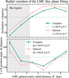 |
Fig. 11 Variation in the LMC disc plane fitting as a function of the LMC galactocentric radius R′. Top: inclination i. Bottom: line-of-nodes position angle Ω. The ‘global’ fit derived in Sect. 4.2 is displayed by the horizontal dashed lines. We use a grey shaded area to draw attention to the bar region (R′bar = 2.3 kpc, Jiménez-Arranz et al. 2023b). In all panels we display the LMC complete (optimal) sample in green (salmon). |
4.4 3D models of the LMC disc
Now that we have determined the viewing angles as function of position, we wish to use this information to construct a three-dimensional (3D) model of the LMC disc. One traditional way to do this is to use the annular fits in Fig. 11, and to represent the LMC disc as a collection of tilted rings. Models based on tilted rings have been used extensively to describe the structure of galaxies, especially by fitting the line-of-sight kinematics of the rings (their rotational and systemic velocities) to the velocity field observed in neutral hydrogen (e.g. Rogstad et al. 1974; Corbelli et al. 2010; Boisvert & Rhee 2016) or other tracers (e.g. Abedi et al. 2014; Jones et al. 2017). In the present paper this kinematic fitting is supplanted by the 3D kinematics modelling that underlies the results in Fig. 11. In the left panels of Fig. 13, we show the LMC tilted ring model using the derived inclination i and the line-of-nodes position angle Ω as function of galactocentric radius R′ from this section – see Fig. 11. We display the LMC Combined complete and optimal samples with green and salmon rings, respectively4.
Tilted ring models have several disadvantages. First, the disc is not represented as a continuous surface, which is unphysical. Second, it is not self-evident how to represent the disc in 3D when the viewing angles are known for disjunct polar segments as in Fig. 12, instead of closed annuli. We therefore developed a new inversion method that takes on input the determinations of the viewing angles on a grid of polar segments (or annuli), and returns on output the continuous surface z′(x′, y′) that best reproduces these viewing angles in a least-squares sense. This method is described in the Appendix A. The middle panels of Fig. 13, show the best-fit LMC disc surfaces obtained with this method given the annular viewing angle results in Fig. 11; similarly, the right panels show the surfaces obtained given the results obtained for the azimuthal wedges in Fig. 12.
The 3D models of the LMC disc in Fig. 13 all reveal that the inner regions are located in a different plane than the disc outskirts, given the variation in the inclination with radius. The models in the right panels further reveal that there is warping in the outer disc, given the variation in the inclination with azimuth. To highlight these features more clearly, we show edge-on views of the 3D inversion-method models in Fig. 14, where edge-on is defined based on the viewing angles determined in Sect. 4.2. We adopt different viewing directions from within this edge-on plane to highlight separately the tilted bar (left, for the models with only radial variations) and the outer warp (right, for the models with both radial and azimuthal variations). The interpretation and origin of these findings is further discussed in Sect. 5.2.
The case that these are real features and are not some observational or analysis artefact is supported by comparison with N-body simulations of the LMC’s interaction with the SMC. Disturbances from the SMC can cause deviations from a flat mid-plane, with the details depending on the exact orbit and impact parameter (Besla et al. 2012). To illustrate this qualitatively, the bottom of Fig. 14 shows edge-on views of two simulated LMCs extracted from the KRATOS simulation suite. These were selected visually from Fig. 3 of Jiménez-Arranz et al. (2024b) for resembling the edge-on views determined here from the data. The similarities are striking, especially given that no attempt was made to quantitatively fit the simulations to these data.
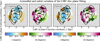 |
Fig. 12 Variation in the LMC disc plane fitting as a function of the azimuth ϕ and the LMC galactocentric radius R′. Left panels: LMC Combined complete sample. Right panels: LMC Combined optimal sample. The first and the third (second and fourth) panels show the inclination i (line-of-nodes position angle Ω). Only bins with more than 50 stars are displayed. Each colour bar is centred on the ‘global’ fit derived in Sect. 4.2. The statistical uncertainties in the displayed quantities depend primarily on the number of stars in each given bin. These uncertainties are much smaller than the spatial variations visible in the maps. The median inclination uncertainty is 1 degree, and the median line-of-nodes position angle uncertainty is 4 degrees. |
 |
Fig. 13 Comparison of 3D models for the LMC disc mid-plane based on the inferred spatial variations in the viewing angle. Left panels: Tilted ring model. Central panels: Inversion method to best fit the inferred viewing angle variations with the galactocentric radius R′ as a continuous surface. Right panels: Inversion method to best fit the inferred viewing angle variations with both the galactocentric radius R′ and azimuth ϕ as a continuous surface. Top panels (green): LMC Combined complete sample. Bottom panels (salmon): LMC Combined optimal sample. We plot a triad that displays the unit vectors in the following directions: W, N, and LOS, being the last the observer’s direction. In the (x, y, z) frame, those vectors are defined by (1, 0, 0), (0, 1, 0), and (0, 0, 1), respectively (see Fig. 11 of Jiménez-Arranz et al. 2023b.) A video of these LMC 3D models viewed from different directions is available online. |
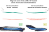 |
Fig. 14 Edge-on view of LMC 3D models. First and second row left panels: inversion method to best fit the inferred viewing angle variations with the galactocentric radius R′ as a continuous surface. First and second right panels: inversion method to best fit the inferred viewing angle variations with both the galactocentric radius R′ and azimuth ϕ as a continuous surface. We plot a triad that displays the unit vectors in the following directions: W, N, and LOS, being the last the observer’s direction. In the (x, y, z) frame, those vectors are defined by (1, 0, 0), (0, 1, 0), and (0, 0, 1), respectively – see Fig. 11 of Jiménez-Arranz et al. (2023b). To best highlight the tilted bar (left) and outer warp (right), the two 3D models are viewed from different angles, with a difference of Δ ϕ = 70∘ in the edge-on plane. Top panels (green): LMC Combined complete sample. Central panels (salmon): LMC Combined optimal sample. Bottom panels: For comparison, two N-body simulated LMC analogues from the KRATOS suite (Jiménez-Arranz et al. 2024b), K15 (left) and K21 (right), respectively. These were selected visually for resembling the edge-on views above determined from the data. |
4.5 Robustness against position of the LMC centre
There has been ongoing discussion about the rotational centre of the LMC for a long time; see for example Fig. 5 of van der Marel & Kallivayalil (2014) or Fig. 10 of Gaia Collaboration (2021b). This problem initially manifested with the photometric centre and the centre of rotation for the HI gas lying at different positions. van der Marel (2001) determined the photometric centre to be (81.28∘, −69.78∘), and also determined that the centre of the outer isopleths, adjusted for viewing angle, to be (82.25∘, −69.50∘). According to Kim et al. (1998), the kinematic centre of the HI gas disc is (79.40∘, −69.03∘), while Luks & Rohlfs (1992) found that it is (78.13∘, −69.00∘). A rotational centre (78.76∘ ± 0.52∘, −69.19∘ ± 0.25∘) that is near the centre of rotation for the HI gas was later determined by van der Marel & Kallivayalil (2014) using Hubble Space Telescope proper motions in the LMC. However, it was noted that this was not consistent with the rotational centre derived from studies of the line-of-sight velocity distribution in carbon stars (van der Marel et al. 2002, e.g. 81.91∘ ± 0.98∘, −69.87∘ ± 0.41∘). Wan et al. (2020) used Gaia DR2 proper motions, along with SkyMapper photometry by Wolf et al. (2018) to find the dynamic centres for carbon stars, RGB stars, and young stars to be (80.90∘ ± 0.29∘, −68.74∘ ± 0.12∘), (81.23∘ ± 0.04∘,−69.00∘ ± 0.02∘), and (80.98∘ ± 0.07∘, −69.69∘ ± 0.02∘), respectively. A kinematical model for the LMC proper motions was fitted using Gaia eDR3 data by Gaia Collaboration (2021b), yielding a centre of (81.01∘, −69.38∘) that is marginally closer to the photometric centre than the HI centre. More recently, Kacharov et al. (2024) using a 3D model of the LMC determined the LMC kinematic centre to be (80.29∘ ± 0.04∘, −69.25∘ ± 0.02∘).
In the present work, we have used the photometric centre, but as discussed, this may not coincide with the kinematic centre. To assess the dependence of our results on the adopted LMC centre, we repeated the analysis of Sect. 4 using the most recent determination of the LMC kinematic centre (80.29∘ ± 0.04∘, −69.25∘ ± 0.02∘) by Kacharov et al. (2024). Their centre is offset by ∼0.55 kpc from the photometric centre.
With this change, we find that all our key requests remain qualitatively unchanged, including the visual appearance of Figs. 4 and 9–12. To get a sense of the quantitative differences, we note that the fits in Sect. 4.1 now yield di/dt = 1.03 ± 0.03 kms−1 kpc−1 (di/dt = 1.32 ± 0.02 kms−1 kpc−1) and dΩ/dt = 3.21 ± 0.07 km s−1 kpc−1 (dΩ/dt = 4.33 ± 0.06 km s−1 kpc−1) for the LMC Combined optimal (complete) sample. If we redo the analysis of Sect. 4.2, for the LMC Combined optimal (complete) sample we now recover a disc plane with inclination i = 23.3∘ ± 0.1∘ (i = 19.5∘ ± 0.1∘) and the line-of-nodes position angle Ω = 329.8∘ ± 0.3∘ (Ω = 332.6∘ ± 0.2∘). The differences compared to the results in those sections are comparable to the differences between the results from the complete and optimal samples. Hence, uncertainties in the position of the LMC centre do not materially alter our results, or our understanding of their systematic uncertainties.
5 Summary and discussion
The objective of this work has been to map the vertical structure of the LMC by combining data from SDSS and Gaia surveys. Motivated by the new line-of-sight velocities from SDSS-V’s Milky Way Mapper (MWM) for a large sample of LMC stars, our goal has been to provide a more comprehensive map of the LMC vertical (off-plane) velocity vz′ than the one provided in Jiménez-Arranz et al. (2023b) just using Gaia DR3 data (see their Fig. 17).
The improvement for this work, with the use of the LMC Combined sample (combination of all line-of-sight velocities available, see Sect. 2), in comparison to Jiménez-Arranz et al. (2023b) comes in the increase of the number of stars by almost a factor of three – see Table 1 for a summary of the numbers of stars per LMC sample. Perhaps even more importantly, the improvement also comes from having a better coverage of the LMC outskirts (see Fig. 1). We validated the reliability of our results regarding the balance between completeness and purity in our samples by conducting the same analysis on the NN complete and optimal LMC clean samples from Jiménez-Arranz et al. (2023b) and finding qualitative agreement. However, in cases where the two samples yield answers for a quantity of interest that differs by more than the statistical uncertainties, we discuss both LMC samples. The difference between the results for the two samples can then be used to assess any systematic uncertainties.
5.1 The LMC’s vertical velocity maps in context
Initially, to create the LMC velocity maps (see Fig. 4), we used the inclination (i = 34∘) and the line-of-nodes position angle (Ω = 310∘) derived in Gaia Collaboration (2021b) and used in Jiménez-Arranz et al. (2023b). To do so, the authors fitted the LMC proper motion as a flat rotating disc, assuming circular orbits. However, instead of using Gaia Collaboration (2021b)’s systemic motion for both proper motion (μα*,0, μδ,0) and line-of-sight velocity (μz,0) values, we re-derived these quantities in this work, because asymmetries in the LMC are well-known (e.g. Besla et al. 2012; Yozin & Bekki 2014; Pardy et al. 2018) and there is variation in the kinematics of different populations (see, for example, Table 1 of Gaia Collaboration 2021b; Dhanush et al. 2024).
With regard to the median vertical velocity maps of the different LMC clean samples (see Sect. 3.1 and Fig. 4), the Combined samples show a trend that is consistent with that reported in the inner regions by the Gaia data (Jiménez-Arranz et al. 2023b), that expands in the outskirts. With half of the galaxy (x′ < 0) moving upwards and the other half (x′ > 0) moving downwards – with respect to the assumed plane of the LMC disc –, the vertical velocity map displays a bimodal trend/dipole. In addition, there appears to be an increasing gradient of vertical velocity magnitude from the inner to the outer disc. As argued in Jiménez-Arranz et al. (2023b), there are (at least) four possible explanations for this: (1) the symmetry axis of the disc is not stationary in an inertial frame due to precession and/or nutation as a result of tidal torques (e.g. Weinberg 2000; van der Marel et al. 2002; Olsen & Massey 2007; Olsen et al. 2011); (2) an incorrect estimation of the disc viewing angles (e.g. Jiménez-Arranz et al. 2023b); (3) the existence of a galactic warp in the LMC’s disc (e.g. Choi et al. 2018; Saroon & Subramanian 2022); (4) the LMC is not in dynamical equilibrium (e.g. Belokurov et al. 2019; Choi et al. 2022; Jiménez-Arranz et al. 2024a,b); or a combination of some/all of these different effects. These hypothesis were tested in Sect. 4, and are discussed further in Sect. 5.2 below.
Interestingly, we found a “blob” of stars with negative vertical velocities in the inner arm’s centre, at roughly (x′, y′) = (−1, −3) kpc (see also Jiménez-Arranz et al. 2023b). This area overlaps with the supershell LMC 4, a high star-forming region of ionised gas approximately ∼1 kpc in size (Tenorio-Tagle & Bodenheimer 1988; Vallenari et al. 2003; Book et al. 2008; Dawson et al. 2013a; Fujii et al. 2014; Ou et al. 2024); this region has been argued to be the LMC’s biggest bubble-like structure – see Fig. 5. We believe this is the first observation of the supershell LMC 4 in the (vertical) kinematics space of resolved LMC stars.
We created the vertical velocity maps for the LMC Combined sample using the different evolutionary phases that are described in Sect. 2.5, to assess how old/young populations manifest in the vertical velocity plane. We split the kinematic tracers into the following stellar types, following the convention from Gaia Collaboration (2021b): Young (Young 1 + Young 2 + Young 3), blue loop (BL), asymptotic giant branch (AGB), and red giant branch (RGB) samples. Overall, the dipole seen in the vertical velocity maps of the Combined sample is observed for the various evolutionary phases of the LMC (see Fig. 6). This indicates that, while different stellar populations could be moving at different vertical velocities, the overall motion of the LMC disc is consistent across all evolutionary phases.
Despite the Young sample being the least represented population, it perfectly traces the supershell LMC 4 observed in the Combined sample. The Young sample is mostly composed by Young 1 stars (see Fig. 3) which corresponds to very young main sequence with ages ≲50 Myr. These stars, as well as the BL sample (with ages ≲300 Myr), are largely observed in the supershell LMC 4 (see Fig. 3 of Gaia Collaboration 2021b). However, this supershell is not seen in the AGB or RGB samples, that are formed by older stars (≲1−2 Gyr). The fact that we see this kinematic feature in young populations and not old ones corroborates that it is connected to the recent star forming region; the ages of stars seen in this population could also serve as a proxy for setting an upper bound on the start of a burst in this region. According to Dopita et al. (1985), star formation appears to have begun close to the centre about ∼15 Myr ago, which is consistent with the age of the stars in our Young sample but not in the BL sample. The authors also discovered three components, two of them being linked to gas shells ejected above and below the LMC disc plane at a velocity of ∼36 km s−1. Our results suggest that we are possibly witnessing this phenomenon, and that it could have potentially begun at an earlier point in time.
Allowing for pure speculation, this kinematic feature could be caused by a potential crossing of the SMC with the LMC disc. This is because it is difficult to obtain high vertical velocity kinematics for a relatively small grouping of young stars in galaxy discs from secular evolution alone. Thus, we argue that our finding of the supershell LMC 4 with high negative vertical kinematics may be the result of one of these interactions between the LMC and SMC. If so, age dating the stellar populations in the LMC 4 supershell structure could help place further constraints on the timing of the interaction between these two sister galaxies. While this scenario is completely speculative at this point in time, it would be an interesting question to entertain in greater detail in future work using numerical simulations.
Additionally, we are able to determine the vertical velocity dispersion and confirm that the Young and BL samples, which represent the younger evolutionary phases, have a smaller velocity dispersion (of the order of ∼5 km s−1) than the AGB and RGB samples, which represent the older evolutionary phases (see Fig. 7). This is to be expected, as older populations have had time to become kinematically hotter than younger populations.
Finally, and for the first time ever, thanks to this wealth of data, we are able to present the one-dimensional vertical velocity profiles as a function of the azimuth, ϕ, defined in the LMC in-plane (x′, y′) Cartesian coordinate system (see Fig. 8). For the Combined sample we observe that the azimuthal wedges along the line-of-nodes (x′ ∼ 0) show a clear trend for the vertical velocity vz′ close to the LMC centre. The right panels of Fig. 4 demonstrate a linear increase (decrease) in the vertical velocity as a function of the LMC galactocentric radius for those wedges. Conversely, the azimuthal wedges that are perpendicular to the line-of-nodes (y′ ∼ 0) exhibit flatter behaviour for all radii. Due to the limited coverage of RGB stars in the LMC centre, we cannot tell if the RGB stars show the observed linear trend of vertical velocity with respect to the galactocentric radius. In the LMC outskirts, however, it displays flattened curves and follows the same pattern as the LMC Combined sample. We can observe the same linear relationship close to the LMC centre for the AGB and BL stars because for these samples the LMC inner region has better coverage than for the outer regions.
5.2 Interpretation of the LMC vertical kinematics
After characterising the LMC vertical kinematic maps for the LMC Combined samples, in Sect. 4 we set out to interpret them. To do so, we conducted three tests: (1) check if the vertical velocity dipole presented in Figs. 4 and 6 could be explained by time variability in the disc symmetry axis (e.g. due to the rate of change in the LMC’s disc viewing angles); (2) re-derive the LMC disc plane by minimising the vertical velocity vz′ across the disc, as the LMC disc plane used in Sect. 3 (namely, the one fitted in Gaia Collaboration 2021b) assumes that stars in the LMC disc are on circular orbits, which may not be the case; (3) re-estimate the values of the inclination angle, i, and the line-of-nodes position angle, Ω, using our data in different bins of galactocentric radius and azimuth. This is because the LMC’s disc could be warped and is therefore not required to be flat and characterised by constant viewing angles.
To undertake the first test, we re-derive a new estimate of the rate of change in the LMC disc viewing angles; namely, the inclination di/dt and the line-of-nodes position angle dΩ/dt, which results in a solid body rotation of the LMC disc. In this work we use a more direct method than the one used in van der Marel et al. (2002); Olsen & Massey (2007); Olsen et al. (2011), where the authors estimated di/dt tailored to a case without astrometric information, and assuming circular orbits to make up for the absence of full 3D velocity info. Since the line-of-sight velocity field does not provide any information on time variations in the position angle of the line of nodes, dΩ/dt, they were unable to provide any estimate for that quantity.
Now, thanks to the astrometric and spectroscopic data provided by the Gaia and SDSS surveys, we have access to the vertical velocities for the LMC disc (Jiménez-Arranz et al. 2023b, and this work), which allows us to estimate di/dt and dΩ/dt using a more direct method. This method involves fitting the LMC vertical velocity under the assumption that the only signal originates from the change in the viewing angles of the LMC disc (see Eq. (1)). Using this method, we obtain di/dt = 0.76 ± 0.03 km s−1 kpc−1 = 45 ± 2∘ Gyr−1 and dΩ/dt = 2.83 ± 0.07 km s−1 kpc−1 = 166 ± 4∘ Gyr−1 for the LMC Combined optimal sample. The results for the LMC Combined complete sample are somewhat different, but also significantly positive for both quantities (see Sect. 4.1). However, for either sample, when we compare the data with the model (see Fig. 9), the residual maps clearly have significant structure that cannot be attributed solely to time-variable viewing angles. Inclusion of non-zero di/dt and dΩ/dt decreases the RMS for the vz′ maps by only ∼1%. Thus, other effects are likely responsible for the structure in the vz′ maps, which could render our determinations of di/dt and dΩ/dt, under the assumptions of a solid rotating body, as meaningless.
With this caveat in mind, it is nonetheless useful to compare our result for di/dt to other estimates in the literature5. First, van der Marel et al. (2002) provided a value of di/dt = −0.37 ± 0.22 mas yr−1 = −103 ± 61∘ Gyr−1 using line-of-sight measurements for 1041 carbon star. Then, Olsen & Massey (2007) and Olsen et al. (2011) with new observations of carbon stars and red supergiants provided an estimates of di/dt = 0.001 mas yr−1 and di/dt = −184 ± 81∘ Gyr−1, respectively. Our results disagree with these values at the ∼3 σ level. However, this is not entirely surprising given the caveats discussed regarding the interpretation of v′z maps. Moreover, we should not expect to obtain the same results as van der Marel et al. (2002) or Olsen et al. (2011) since the underlying kinematical assumptions are different. Our method is based on the velocities perpendicular to the plane, whereas those papers assumed that the orbits in the plane are purely circular.
Theoretical estimates of the rates of change in the LMC disc viewing angles with numerical models (e.g. Weinberg 2000) are left for future work. This could be addressed with the KRATOS (Jiménez-Arranz et al. 2023a) simulations, for example. KRATOS is a comprehensive suite of 28 pure N-body simulations of isolated and interacting LMC-like galaxies devoted to study the formation of substructures in their disc after the interaction with an SMC-mass galaxy, or by identifying LMC analogues in cosmological simulations (e.g. Boylan-Kolchin et al. 2011; Sales et al. 2011; Santos-Santos et al. 2021; Buch et al. 2024). We reserve this exploration for future work.
After discarding any time variability in the LMC disc viewing angles as the main reason for the dipole and structure in the vertical velocity maps, we considered alternative explanations. Since the analysis above was conducted under the assumption that the LMC disc plane fitted in Gaia Collaboration (2021b) was the actual LMC disc plane, this could yield a biased answer because of the assumption of circular orbits. To test whether this assumption is indeed biasing our results, we re-derived the orientation of the LMC disc plane by minimising the RMS vertical velocity vz′ across the disc of the LMC (see Sect. 4.2). For the LMC Combined optimal (complete) sample, we recover a disc plane with inclination i = 23.6∘ ± 0.1∘ (i = 20.0∘ ± 0.1∘) and the line-of-nodes position angle Ω = 326.9∘ ± 0.3∘ (Ω = 330.0∘ ± 0.2∘). Compared to the LMC disc plane fitting of Gaia Collaboration (2021b), with i = 34∘ and Ω = 310∘, the LMC disc plane inclination and the line-of-nodes position angle that we recover for the LMC Combined optimal (complete) sample differ by δi ∼ 10∘ (δi ∼ 14∘) and δ Ω ∼ 17∘ (δ Ω ∼20∘). The values we obtained are consistent with the low-end of the wide range of estimates found in the literature (e.g. van der Marel et al. 2009; van der Marel & Kallivayalil 2014; Haschke et al. 2012; Ripepi et al. 2022; Kacharov et al. 2024).
When analysing the new kinematic maps with the new fitted values of i and Ω in this work (see Fig. 10), we observe that: (1) the LMC bar major axis becomes less aligned with the line-of-nodes due to the change of plane – we note that there is no physical reason for both axes being aligned; (2) the LMC’s bar bimodal vertical velocity trend vanishes, leaving behind a nearly null median vertical velocity; (3) there is a sign change in the disc’s vertical velocity bimodal trend; (4) the supershell LMC 4 continues to stand out from the background, albeit not as much as with the LMC disc plane fitted in Gaia Collaboration (2021b). We found that a different disc orientation (although relatively similar) than the one suggested by Gaia Collaboration (2021b) minimises the overall vertical velocities. However, even with that new orientation a clear dipole pattern remains visible in the vertical velocity maps.
We therefore undertook a third test to investigate whether this may be due to warps or twists in the LMC disc plane. To do so, we repeated the best fit disc plane minimisation of Sect. 4.2 for different annular rings in the (x′, y′) plane – defined by the inclination angle, i, and the line-of-nodes position angle, Ω, of Gaia Collaboration (2021b) – to quantify the change of (i, Ω) as function of the LMC galactocentric radial position R′ (see Fig. 11 left panels). We observed that in both samples the inclination is low (i ∼ 10∘) at the inner regions (R′ ∼ 0 kpc) and grows up to values of i ∼ 25∘ for the outer disc (R′ ≳ 3.5 kpc). The line-of-nodes position angle in both samples is high (Ω ∼ 335∘ − 350∘) at the inner regions (R′ ∼ 0 kpc), decreases to values of Ω ∼320∘ − 325∘ at approximately R′ ∼ 2.5 kpc, and then increases once more to values of Ω ∼335∘ in the outer disc (R′ ≳ 3.5 kpc). For both inclination and the line-of-nodes position angle, the LMC Combined complete and optimal samples have a small and almost constant offset from each other. Regardless, the important result from these findings is that the LMC disc is not flat.
Other observational studies have also found radial variations in the disc viewing angles in support of warps and twists in the LMC disc, but the results are not always mutually consistent. van der Marel & Cioni (2001) performed a photometric study of tracer brightnesses as function of position on the sky. They found a decrease in inclination from i ∼ 40∘ just outside the bar to i ∼ 30∘ for the outer disc, as well as a gradual decrease in the position angle of the line-of-nodes. The declining inclination trend in the outer regions may be consistent with our findings, albeit with a smaller amplitude. However, we find an increase in the line-of-nodes position angle with at large radii, instead of a decrease. Compared to the “global” fit presented in this work (i ∼ 20−23∘), the inclination derived in van der Marel & Cioni (2001) is larger (i ∼ 35∘), and the line-of-nodes position angle lower (Ω ∼ 303∘), both being more comparable to the values from Gaia Collaboration (2021b). The photometric study of Choi et al. (2018) ignored the innermost regions of the LMC disc. Beyond that, in contrast to our findings and more similar to the photometric results of van der Marel & Cioni (2001), they inferred that the inclination decreases as a function of radius, beginning at i ∼ 40∘ (see also Dhanush et al. 2024). However, more similar to our findings, the authors found a decreasing trend as function of radius for the line-of-nodes position angle beyond the bar, as shown in Fig. 11. Our work and the literature may yield different results because of the different underlying assumptions. The majority of the literature determines the LMC plane by means of photometric methods (e.g. van der Marel & Cioni 2001; Choi et al. 2018), which make assumptions related to the influence of dust extinction and of spatial age and population gradients. Another common method to determine the LMC plane is done by fitting a kinematic model (e.g. Gaia Collaboration 2021b; Dhanush et al. 2024) that assumes purely circular orbits. In our case, we determine the LMC disc inclination and the line-of-nodes position angle by minimising the vertical velocity.
We also quantified the change of (i, Ω) as a function of both the LMC azimuth ϕ and galactocentric radial position R′ by repeating the best disc plane fitting in annular wedges (see Fig. 12). In agreement with the annular fits, both the LMC Combined complete and optimal sample display a fairly homogeneous and isotropic central part of the disc with a low inclination i and a high line-of-nodes position angle Ω. However, we observe a quadrupolar pattern for both angles (i, Ω) in the outer regions, with a significant variation as a function of the azimuth ϕ. This is a clear sign of a warp in the LMC disc plane.
The inferred spatially variable viewing angles have enabled us to construct three-dimensional models of the shape of the LMC disc plane, using both the LMC Combined complete and optimal samples (see Fig. 13). For this we have used both traditional tilted-ring models, as well as a new inversion method described in the Appendix A. The 3D models show that the inner regions are located in a different plane than the disc outskirts, given the difference in inclination found between the inner and outer regions of the LMC disc. This could be due to an inclination of the bar relative to the disc plane (e.g. Subramaniam 2003; Besla et al. 2012; Choi et al. 2018). Simulations of the LMC-SMC interaction by Besla et al. (2012) indeed found a 5∘–15∘ tilted bar with regard to the LMC disc, if the SMC recently passed through the LMC disc. Choi et al. (2018) postulated that such a tilt was consistent with the observed spatial variations in the magnitude of red clump stars. Choi et al. (2022) reported additional evidence for a recent SMC collision with a small impact parameter, which could induce a warp in the LMC disc (e.g. Kim et al. 2014; Semczuk et al. 2020; Wille & Machado 2024). Our results provide further support for these findings. However, it must be noted that other effects associated with disequilibrium (e.g. Belokurov et al. 2019; Choi et al. 2022; Jiménez-Arranz et al. 2024a,b) may play a role as well. Previous authors have found evidence for a warp in the outer regions of the LMC disc (e.g. van der Marel et al. 2002; Olsen & Salyk 2002; Nikolaev et al. 2004; Choi et al. 2018; Ripepi et al. 2022). Our 3D models support this, given the variation in the inclination with azimuth found in the disc. The appearance of an inclined bar could merely be a natural extension of this warp, instead of a separate physical effect.
6 Conclusions
The aim of this work was to map the vertical structure of the LMC by combining data from SDSS and Gaia surveys. This was motivated by the new line-of-sight velocities from SDSS-V’s MWM for a large sample of LMC stars. These new data enabled the construction of a more comprehensive map of the LMC vertical (off-plane) velocity vz′ than the one provided in Jiménez-Arranz et al. (2023b) using only Gaia DR3 data (see their Fig. 17). With this improved map, we were able to perform a comprehensive investigation of the 3D shape of the LMC disc plane and of the orientation of its symmetry axis as well as any time variability therein. The main results shown in this paper are summarised as follows:
We increased the number of LMC stars with line-of-sight velocity information by almost a factor of three compared to Jiménez-Arranz et al. (2023b). Even more importantly, we have better coverage of the LMC disc outskirts. With these data, we cover a projected radius of R ≲ 5 kpc (see Fig. 1);
We provided the first identification of the supershell LMC 4 in the (vertical) kinematics space of resolved LMC stars (see Figs. 4–7). When examining various stellar populations, we observed that LMC 4 is only discernible for stars younger than ∼300 Myr (see Fig. 6). We speculate that this might be an aftermath of the recent LMC-SMC interaction, which will be investigated in a future work;
In agreement with Jiménez-Arranz et al. (2023b), but expanding the trend in the outskirts of the LMC, half of the galaxy moves upwards and the other half moves downward, |vz′| ≈ 10−15 km s−1, with respect to the fitted plane of the LMC disc provided by Gaia Collaboration (2021b, see Figs. 4 and 8). This is also the case when examining the profile for stars at different evolutionary stages;
We interpret this bimodal trend in the LMC vertical velocity map with three distinct possibilities: 1) time variation in the orientation of the disc symmetry axis (e.g. due to precession or nutation); 2) use of an incorrect LMC disc plane; and 3) the presence of warps and twists in the LMC disc;
1) We fitted for time variation in the disc viewing angles and obtained non-zero results, namely, di/dt = 0.76 ± 0.03 km s−1 kpc−1 = 45 ± 2∘ Gyr−1 and dΩ/dt = 2.83 ± 0.07 km s−1 kpc−1 = 166 ± 4∘ Gyr−1, for the LMC Combined optimal sample (see Fig. 9). However, these results may be spurious since most of the structure in the vertical velocity maps remains even when these fitted values are included. Thus, time variation in the orientation of the disc symmetry axis does not explain the inferred velocity dipole; 2) We re-derived the orientation of the LMC disc plane by minimising the RMS vertical velocity vz′ across the disc of the LMC. For the LMC Combined optimal sample, we recovered a disc plane with an inclination of i = 23.6∘ ± 0.1∘ and a line-of-nodes position angle of Ω = 326.9∘ ± 0.3∘ (see Fig. 10). The results for the LMC Combined complete sample differ by ∼3∘, which provides an indication of the systematic uncertainty in these determinations. Changes in the adopted position of the LMC centre can affect the results at similar levels;
3) We repeated the plane fitting for different annular rings in the LMC disc (see Fig. 11). The results imply a difference in inclination between the inner and outer regions of the LMC disc, which is qualitatively consistent with a 5∘ − 15∘ tilted bar with regard to the LMC disc as seen in simulations by Besla et al. (2012) and supported observationally by Choi et al. (2018). We also quantified the change in the viewing angles as a function of both azimuth and galactocentric radius (see Fig. 12). This yielded a quadrupolar pattern for both viewing angles in the outer disc. The variations as a function of azimuth imply the presence of a warp in the outer LMC disc plane;
We presented a new inversion method to use the results from the aforementioned analyses to construct 3D representations of the shape of the LMC disc plane (see Figs. 13 and 14). We presented the results from this method and compared them to more traditional tilted-ring representations. The 3D representations revealed that the LMC disc is not a flat plane in equilibrium but that the central bar region is tilted relative to a warped outer disc. These data provide further evidence for perturbations caused by interaction with the SMC.
In summary, the currently available SDSS and Gaia dataset has proven suitable for studies of the LMC out-of-plane kinematics and 3D structure. Future releases of surveys such as SDSS, Gaia (DR4), and 4MOST may allow this work to be revisited once more line-of-sight velocities are available in the LMC.
Data availability
The movie associated to Fig. 13 is available at https://www.aanda.org
Movie
Movie associated to Fig. 13 Access Supplementary Material
Acknowledgements
We thank the referee for valuable suggestions that helped to improve the manuscript. We are grateful to M. Romero-Gómez, X. Luri, K. V. Johnston, E. Cunningham, H. Rathore, and J. G. Fernández-Trincado for fruitful discussions. OJA acknowledges funding from “Swedish National Space Agency 2023-00154 David Hobbs The GaiaNIR Mission” and “Swedish National Space Agency 2023-00137 David Hobbs The Extended Gaia Mission”. DH acknowledges support from the Flatiron Institute, funded by the Simons Foundation. CL acknowledges funding from the European Research Council (ERC) under the European Union’s Horizon 2020 research and innovation programme (grant agreement No. 852839). Funding for the Sloan Digital Sky Survey V has been provided by the Alfred P. Sloan Foundation, the Heising-Simons Foundation, the National Science Foundation, and the Participating Institutions. SDSS acknowledges support and resources from the Center for High-Performance Computing at the University of Utah. SDSS telescopes are located at Apache Point Observatory, funded by the Astrophysical Research Consortium and operated by New Mexico State University, and at Las Campanas Observatory, operated by the Carnegie Institution for Science. The SDSS web site is www.sdss.org. SDSS is managed by the Astrophysical Research Consortium for the Participating Institutions of the SDSS Collaboration, including the Carnegie Institution for Science, Chilean National Time Allocation Committee (CNTAC) ratified researchers, Caltech, the Gotham Participation Group, Harvard University, Heidelberg University, The Flatiron Institute, The Johns Hopkins University, L’Ecole polytechnique fédérale de Lausanne (EPFL), Leibniz-Institut für Astrophysik Potsdam (AIP), Max-Planck-Institut für Astronomie (MPIA Heidelberg), Max-Planck-Institut für Extraterrestrische Physik (MPE), Nanjing University, National Astronomical Observatories of China (NAOC), New Mexico State University, The Ohio State University, Pennsylvania State University, Smithsonian Astrophysical Observatory, Space Telescope Science Institute (STScI), the Stellar Astrophysics Participation Group, Universidad Nacional Autónoma de México, University of Arizona, University of Colorado Boulder, University of Illinois at Urbana-Champaign, University of Toronto, University of Utah, University of Virginia, Yale University, and Yunnan University. This work has made use of data from the European Space Agency (ESA) mission Gaia (https://www.cosmos.esa.int/gaia), processed by the Gaia Data Processing and Analysis Consortium (DPAC, https://www.cosmos.esa.int/web/gaia/dpac/consortium). Funding for the DPAC has been provided by national institutions, in particular the institutions participating in the Gaia Multilateral Agreement.
Appendix A Determination of 3D LMC shape
Figure 12 shows determinations of the LMC viewing angles i and Ω on a polar grid in the (x′, y′) plane. The grid consists of segments that have their centres at radii  for l = 1, … L and
  for m = 1, … M. Here R′ is the cylindrical radius in the (x′, y′) plane, and ϕ′ the azimuthal angle in that plane measured counter-clockwise from the x′-axis. In practice, we take Δ R′ = 1 kpc with L = 6 and Δ R′ = 360∘/M, with M = 12. For the discussion below we group the innermost M azimuthal segments into a single filled circle of radius Δ R′, centred on R′ = 0. There are then a total of Nseg = 1 + (L−1) M segments.
On each individual segment n = 1, …, Nseg the LMC disc is described by a plane of the form  . Here
  is the centre of the segment in the 3D (x′, y′, z′) coordinate space. The normal vector to this plane is (an, bn, −1). This normal vector is fully defined by the viewing angles in and Ωn for the given segment, so that the an and bn are known through the transformation equations given in van der Marel (2001) and van der Marel et al. (2002). However, the
  for n = 1, …, Nseg are unknown and need to be determined to fully describe the three-dimensional shape of the LMC disc.
To determine the  we enforce the constraint that the disc be continuous at the segment boundaries. The boundaries between adjacent segments within the same annulus are centred on the points with polar coordinates
  as defined above for l = 2, … L and
  for k = 1, … M. The boundaries between adjacent segments in adjacent annuli are centred on the points with polar coordinates
  for j = 1, … L − 1 and
  as define above for m = 1, … M. The are a total of of Nbound = 2(L − 1) M of such boundary centres. To lowest order, there are about twice as many boundary centres as segment centres.
For each boundary centre i = 1, …, Nbound there are two adjacent segments n1 and n2 that touch, with n1 and n2 in the range 1, …, Nseg. To get any two adjacent segments to yield the same value of z′ at their boundary centre, the following equations must be satisfied for i = 1, …, Nbound:
 (A.1)
(A.1)
The right-hand side is known for each i and its corresponding n1 and n2, whereas the left-hand side contains two of the unknowns. This set of equations can be expressed as a matrix equation of the form Az = c. Here A is a sparse Nbound × Nseg matrix with only elements +1, −1, and 0; c is the Nbound vector composed of the right-hand sides of equation (A.1); and z′ is the Nseg vector composed of the unknown zcen,n′ for n=1, …, Nseg.
The aforementioned matrix equation Az′ = c is an overdetermined equation since Nbound > Nseg.. It generally has a well-defined solution in a least-squares sense, apart from the onedimensional degeneracy that for any solution vector  , the addition of the same constant to all the vector elements also yields a solution vector. In other words, while we can determine the 3D shape of the LMC disc given i and Ω on a polar grid, we cannot determine its distance. We solve this degeneracy by forcing the average of the elements of
  to be zero. The solution can then be determined using singular-value decomposition of the matrix A, which was implemented in FORTRAN using subroutines from Press et al. (1992).
After having determined the  on the polar grid for n = 1, …, Nseg, we use bi-cubic interpolation on the polar grid (also using subroutines from Press et al. 1992) to allow evaluation of the surface z′(x′, y′) for arbitrary (x′, y′). This yields a continuous representation of the LMC disc that best matches the (i, Ω)n for n = 1, …, Nseg determined on a polar grid as described in Sect. 4.3. Once we have the bi-cubic interpolation, we can numerically determine the normal vector to the surface at the segment centres. Using the transformation equations given in van der Marel (2001) and van der Marel et al. (2002), this yields the (i, Ω)fit,n of the fitted surface.
The fitted (i, Ω)fit,n do not generally reproduce the input (i, Ω)n exactly, but they provide the best possible match with a continuous disc surface in the sense described above. As discussed in Sect. 4.3, for our real LMC data there are significant residuals, but the fitted (i, Ω)fit maps do capture the qualitative essence of the input (i, Ω) maps.
The entire numerical implementation of the aforementioned algorithm was tested and validated by having it successfully recover known analytical surfaces from gridded (i, Ω)fit,n pseudoinput data generated from those surfaces.
The formalism described above can also be used to generate 3D renditions of the LMC disc for the situation of Sect. 4.2, in which the LMC viewing angles i and Ω were fitted over annuli. In this case we use the same polar grid as described above, with M = 12. But we set the input viewing angles to be the same for all segments within the same annulus. In this case we find that to maintain continuity, the fitted (i, Ω)fit do not have the same values for all segments within the same annulus. This is because by its very nature, a tilted-ring model is a disjunct, and not a continuous representation of a disc.
Appendix B Comparison of the LMC complete and optimal sample
As mentioned at the end of Sect. 2.4, the two samples (LMC complete and optimal) produce qualitatively similar results for the majority of the figures and analyses in this paper. As a result, we typically only display results for the optimal sample. The comparison of the LMC complete and optimal samples which correspond to Figs. 3, 6, 7, and 8, is displayed in Figs. B.1, B.2, B.3, and B.4 of this Appendix, respectively.
References
- Abdurro’uf, Accetta, K., Aerts, C., et al. 2022, ApJS, 259, 35 [NASA ADS] [CrossRef] [Google Scholar]
- Abedi, H., Mateu, C., Aguilar, L. A., Figueras, F., & Romero-Gómez, M., 2014, MNRAS, 442, 3627 [NASA ADS] [CrossRef] [Google Scholar]
- Almeida, A., Anderson, S. F., Argudo-Fernández, M., et al. 2023, ApJS, 267, 44 [NASA ADS] [CrossRef] [Google Scholar]
- Avner, E. S., & King, I. R., 1967, AJ, 72, 650 [Google Scholar]
- Belokurov, V., Deason, A. J., Erkal, D., et al. 2019, MNRAS, 488, L47 [Google Scholar]
- Besla, G., Kallivayalil, N., Hernquist, L., et al. 2012, MNRAS, 421, 2109 [Google Scholar]
- Blanton, M. R., Bershady, M. A., Abolfathi, B., et al. 2017, AJ, 154, 28 [Google Scholar]
- Boisvert, J. H., & Rhee, G., 2016, AJ, 152, 15 [Google Scholar]
- Book, L. G., Chu, Y.-H., & Gruendl, R. A., 2008, ApJS, 175, 165 [NASA ADS] [CrossRef] [Google Scholar]
- Bowen, I. S., & Vaughan, A. H., J. 1973, Appl. Opt., 12, 1430 [NASA ADS] [CrossRef] [Google Scholar]
- Boylan-Kolchin, M., Besla, G., & Hernquist, L., 2011, MNRAS, 414, 1560 [NASA ADS] [CrossRef] [Google Scholar]
- Buch, D., Nadler, E. O., Wechsler, R. H., & Mao, Y.-Y., 2024, ApJ, 971, 79 [Google Scholar]
- Choi, Y., Nidever, D. L., Olsen, K., et al. 2018, ApJ, 866, 90 [Google Scholar]
- Choi, Y., Olsen, K. A. G., Besla, G., et al. 2022, ApJ, 927, 153 [NASA ADS] [CrossRef] [Google Scholar]
- Cioni, M. R. L., Clementini, G., Girardi, L., et al. 2011, A&A, 527, A116 [CrossRef] [EDP Sciences] [Google Scholar]
- Corbelli, E., Lorenzoni, S., Walterbos, R., Braun, R., & Thilker, D., 2010, A&A, 511, A89 [NASA ADS] [CrossRef] [EDP Sciences] [Google Scholar]
- Cropper, M., Katz, D., Sartoretti, P., et al. 2018, A&A, 616, A5 [NASA ADS] [CrossRef] [EDP Sciences] [Google Scholar]
- Cullinane, L. R., Mackey, A. D., Da Costa, G. S., et al. 2022a, MNRAS, 510, 445 [Google Scholar]
- Cullinane, L. R., Mackey, A. D., Da Costa, G. S., et al. 2022b, MNRAS, 512, 4798 [NASA ADS] [CrossRef] [Google Scholar]
- Cusano, F., Moretti, M. I., Clementini, G., et al. 2021, MNRAS, 504, 1 [NASA ADS] [CrossRef] [Google Scholar]
- Dawson, J. R., McClure-Griffiths, N. M., Wong, T., et al. 2013a, ApJ, 763, 56 [NASA ADS] [CrossRef] [Google Scholar]
- Dawson, K. S., Schlegel, D. J., Ahn, C. P., et al. 2013b, AJ, 145, 10 [Google Scholar]
- De Angeli, F., Weiler, M., Montegriffo, P., et al. 2023, A&A, 674, A2 [NASA ADS] [CrossRef] [EDP Sciences] [Google Scholar]
- de Jong, R. S., Agertz, O., Berbel, A. A., et al. 2019, The Messenger, 175, 3 [NASA ADS] [Google Scholar]
- de Vaucouleurs, G., & Freeman, K. C., 1972, Vistas Astron., 14, 163 [Google Scholar]
- Dhanush, S. R., Subramaniam, A., & Subramanian, S., 2024, ApJ, 968, 103 [Google Scholar]
- Dopita, M. A., Mathewson, D. S., & Ford, V. L., 1985, ApJ, 297, 599 [Google Scholar]
- Eisenstein, D. J., Weinberg, D. H., Agol, E., et al. 2011, AJ, 142, 72 [Google Scholar]
- Elmegreen, D. M., & Elmegreen, B. G., 1980, AJ, 85, 1325 [NASA ADS] [CrossRef] [Google Scholar]
- Erkal, D., Belokurov, V., Laporte, C. F. P., et al. 2019, MNRAS, 487, 2685 [Google Scholar]
- Fujii, K., Minamidani, T., Mizuno, N., et al. 2014, ApJ, 796, 123 [Google Scholar]
- Gaia Collaboration (Prusti, T., et al.,) 2016, A&A, 595, A1 [NASA ADS] [CrossRef] [EDP Sciences] [Google Scholar]
- Gaia Collaboration (Brown, A. G. A., et al.,) 2018a, A&A, 616, A1 [NASA ADS] [CrossRef] [EDP Sciences] [Google Scholar]
- Gaia Collaboration (Helmi, A., et al.,) 2018b, A&A, 616, A12 [NASA ADS] [CrossRef] [EDP Sciences] [Google Scholar]
- Gaia Collaboration (Brown, A. G. A., et al.,) 2021a, A&A, 649, A1 [NASA ADS] [CrossRef] [EDP Sciences] [Google Scholar]
- Gaia Collaboration (Luri, X., et al.,) 2021b, A&A, 649, A7 [EDP Sciences] [Google Scholar]
- Gaia Collaboration (Drimmel, R., et al.,) 2023a, A&A, 674, A37 [CrossRef] [EDP Sciences] [Google Scholar]
- Gaia Collaboration (Vallenari, A., et al.,) 2023b, A&A, 674, A1 [NASA ADS] [CrossRef] [EDP Sciences] [Google Scholar]
- Gallagher, John S., I., & Hunter, D. A. 1984, ARA&A, 22, 37 [NASA ADS] [CrossRef] [Google Scholar]
- Gunn, J. E., Siegmund, W. A., Mannery, E. J., et al. 2006, AJ, 131, 2332 [NASA ADS] [CrossRef] [Google Scholar]
- Haschke, R., Grebel, E. K., & Duffau, S., 2012, AJ, 144, 106 [NASA ADS] [CrossRef] [Google Scholar]
- Ivezić, Ž., Kahn, S. M., Tyson, J. A., et al. 2019, ApJ, 873, 111 [Google Scholar]
- Jiménez-Arranz, Ó., Romero-Gómez, M., Luri, X., & Masana, E. 2023a, A&A, 672, A65 [NASA ADS] [CrossRef] [EDP Sciences] [Google Scholar]
- Jiménez-Arranz, Ó., Romero-Gómez, M., Luri, X., et al. 2023b, A&A, 669, A91 [NASA ADS] [CrossRef] [EDP Sciences] [Google Scholar]
- Jiménez-Arranz, Ó., Chemin, L., Romero-Gómez, M., et al. 2024a, A&A, 683, A102 [NASA ADS] [CrossRef] [EDP Sciences] [Google Scholar]
- Jiménez-Arranz, Ó., Roca-Fàbrega, S., Romero-Gómez, M., et al. 2024b, A&A, 688, A51 [NASA ADS] [CrossRef] [EDP Sciences] [Google Scholar]
- Jones, G. C., Carilli, C. L., Shao, Y., et al. 2017, ApJ, 850, 180 [Google Scholar]
- Kacharov, N., Tahmasebzadeh, B., Cioni, M.-R. L., et al. 2024, A&A, 692, A40 [NASA ADS] [CrossRef] [EDP Sciences] [Google Scholar]
- Katz, D., Munari, U., Cropper, M., et al. 2004, MNRAS, 354, 1223 [NASA ADS] [CrossRef] [Google Scholar]
- Katz, D., Sartoretti, P., Guerrier, A., et al. 2023, A&A, 674, A5 [NASA ADS] [CrossRef] [EDP Sciences] [Google Scholar]
- Kim, S., Staveley-Smith, L., Dopita, M. A., et al. 1998, ApJ, 503, 674 [Google Scholar]
- Kim, J. H., Peirani, S., Kim, S., et al. 2014, ApJ, 789, 90 [NASA ADS] [CrossRef] [Google Scholar]
- Kollmeier, J. A., Zasowski, G., Rix, H.-W., et al. 2017, arXiv e-prints [arXiv:1711.03234] [Google Scholar]
- Kollmeier, J., Anderson, S. F., Blanc, G. A., et al. 2019, in Bulletin of the American Astronomical Society, 51, 274 [Google Scholar]
- Lindegren, L., Klioner, S. A., Hernández, J., et al. 2021, A&A, 649, A2 [EDP Sciences] [Google Scholar]
- Luks, T., & Rohlfs, K., 1992, A&A, 263, 41 [NASA ADS] [Google Scholar]
- Maia, F. F. S., Dias, B., Santos, J. F. C., et al. 2019, MNRAS, 484, 5702 [Google Scholar]
- Majewski, S. R., Schiavon, R. P., Frinchaboy, P. M., et al. 2017, AJ, 154, 94 [NASA ADS] [CrossRef] [Google Scholar]
- Nelder, J. A., & Mead, R., 1965, Comput. J., 7, 308 [Google Scholar]
- Nidever, D., 2021, https://doi.org/10.5281/zenodo.4906681 [Google Scholar]
- Nidever, D. L., Holtzman, J. A., Allende Prieto, C., et al. 2015, AJ, 150, 173 [NASA ADS] [CrossRef] [Google Scholar]
- Nidever, D. L., Olsen, K., Walker, A. R., et al. 2017, AJ, 154, 199 [Google Scholar]
- Nidever, D. L., Hasselquist, S., Hayes, C. R., et al. 2020, ApJ, 895, 88 [Google Scholar]
- Niederhofer, F., Cioni, M.-R. L., Schmidt, T., et al. 2022, MNRAS, 512, 5423 [NASA ADS] [CrossRef] [Google Scholar]
- Nikolaev, S., Drake, A. J., Keller, S. C., et al. 2004, ApJ, 601, 260 [NASA ADS] [CrossRef] [Google Scholar]
- Olsen, K. A. G., & Massey, P., 2007, ApJ, 656, L61 [NASA ADS] [CrossRef] [Google Scholar]
- Olsen, K. A. G., & Salyk, C., 2002, AJ, 124, 2045 [NASA ADS] [CrossRef] [Google Scholar]
- Olsen, K. A. G., Zaritsky, D., Blum, R. D., Boyer, M. L., & Gordon, K. D., 2011, ApJ, 737, 29 [CrossRef] [Google Scholar]
- Ou, P.-S., Chao, R.-C., Chu, Y.-H., Hsu, C.-Y., & Li, C.-J. 2024, AJ, 168, 33 [Google Scholar]
- Pardy, S. A., D’Onghia, E., & Fox, A. J., 2018, ApJ, 857, 101 [NASA ADS] [CrossRef] [Google Scholar]
- Peñarrubia, J., Gómez, F. A., Besla, G., Erkal, D., & Ma, Y.-Z. 2016, MNRAS, 456, L54 [CrossRef] [Google Scholar]
- Pietrzyński, G., Graczyk, D., Gallenne, A., et al. 2019, Nature, 567, 200 [Google Scholar]
- Povick, J. T., Nidever, D. L., Massana, P., et al. 2023, arXiv e-prints [arXiv:2310.14299] [Google Scholar]
- Povick, J. T., Nidever, D. L., Massana, P., et al. 2024, MNRAS, 533, 3685 [Google Scholar]
- Press, W. H., Teukolsky, S. A., Vetterling, W. T., & Flannery, B. P., 1992, Numerical recipes in FORTRAN. The art of scientific computing (Cambridge: University Press) [Google Scholar]
- Rathore, H., Choi, Y., Olsen, K. A. G., & Besla, G., 2025, ApJ, 978, 55 [Google Scholar]
- Ricker, G. R., Winn, J. N., Vanderspek, R., et al. 2015, J. Astron. Telesc. Instrum. Syst., 1, 014003 [Google Scholar]
- Ripepi, V., Chemin, L., Molinaro, R., et al. 2022, MNRAS, 512, 563 [NASA ADS] [CrossRef] [Google Scholar]
- Rogstad, D. H., Lockhart, I. A., & Wright, M. C. H., 1974, ApJ, 193, 309 [Google Scholar]
- Sales, L. V., Navarro, J. F., Cooper, A. P., et al. 2011, MNRAS, 418, 648 [CrossRef] [Google Scholar]
- Santos-Santos, I. M. E., Fattahi, A., Sales, L. V., & Navarro, J. F., 2021, MNRAS, 504, 4551 [NASA ADS] [CrossRef] [Google Scholar]
- Saroon, S., & Subramanian, S., 2022, A&A, 666, A103 [NASA ADS] [CrossRef] [EDP Sciences] [Google Scholar]
- Schlegel, D., White, M., & Eisenstein, D., 2009, in astro2010: The Astronomy and Astrophysics Decadal Survey, 2010, 314 [Google Scholar]
- Semczuk, M., Łokas, E. L., D’Onghia, E., et al. 2020, MNRAS, 498, 3535 [NASA ADS] [CrossRef] [Google Scholar]
- Smee, S. A., Gunn, J. E., Uomoto, A., et al. 2013, AJ, 146, 32 [Google Scholar]
- Sparke, L. S., & Gallagher, John S., III 2000, Galaxies in the universe: an introduction (Cambridge, UK: Cambridge University Press) [Google Scholar]
- Subramaniam, A., 2003, ApJ, 598, L19 [NASA ADS] [CrossRef] [Google Scholar]
- Tenorio-Tagle, G., & Bodenheimer, P., 1988, ARA&A, 26, 145 [NASA ADS] [CrossRef] [Google Scholar]
- Vallenari, A., Moretti, A., Held, E., Rizzi, L., & Bettoni, D., 2003, in Astronomical Society of the Pacific Conference Series, 296, New Horizons in Globular Cluster Astronomy, eds. G. Piotto, G. Meylan, S. G. Djorgovski, & M. Riello, 507 [Google Scholar]
- van der Marel, R. P., 2001, AJ, 122, 1827 [Google Scholar]
- van der Marel, R. P., & Cioni, M.-R. L., 2001, AJ, 122, 1807 [Google Scholar]
- van der Marel, R. P., & Kallivayalil, N., 2014, ApJ, 781, 121 [Google Scholar]
- van der Marel, R. P., & Sahlmann, J., 2016, ApJ, 832, L23 [CrossRef] [Google Scholar]
- van der Marel, R. P., Alves, D. R., Hardy, E., & Suntzeff, N. B., 2002, AJ, 124, 2639 [NASA ADS] [CrossRef] [Google Scholar]
- van der Marel, R. P., Kallivayalil, N., & Besla, G., 2009, in IAU Symposium, Vol. 256, The Magellanic System: Stars, Gas, and Galaxies, eds. J. T. Van Loon & J. M. Oliveira, 81 [Google Scholar]
- Virtanen, P., Gommers, R., Oliphant, T. E., et al. 2020, Nat. Methods, 17, 261 [Google Scholar]
- Wan, Z., Guglielmo, M., Lewis, G. F., Mackey, D., & Ibata, R. A., 2020, MNRAS, 492, 782 [Google Scholar]
- Weinberg, M. D., 2000, ApJ, 532, 922 [Google Scholar]
- Wille, A., & Machado, R. E. G., 2024, MNRAS, 533, 2997 [Google Scholar]
- Wilson, J. C., Hearty, F. R., Skrutskie, M. F., et al. 2019, PASP, 131, 055001 [NASA ADS] [CrossRef] [Google Scholar]
- Wolf, C., Onken, C. A., Luvaul, L. C., et al. 2018, PASA, 35, e010 [Google Scholar]
- Yozin, C., & Bekki, K., 2014, MNRAS, 439, 1948 [Google Scholar]
- Zaritsky, D., 2004, ApJ, 614, L37 [NASA ADS] [CrossRef] [Google Scholar]
This is because the survey is not yet complete. As more data is collected, the missing patches observed across the LMC’s disc will be filled in.
As shown in Fig. 11 of Jiménez-Arranz et al. (2023b), negative vertical velocities vz′ represent a motion compatible with moving away from the observer (MW).
We note that Ω, introduced in Gaia Collaboration (2018b, 2021b), differs from the angle Θ defined by van der Marel & Cioni (2001) and used by other authors by 180 degrees.
A video of the LMC 3D models from different viewing angles is made available online. Additionally, https://www.oscarjimenezar ranz.com/visualizations/interactive-lmc-3d-models offers an interactive version of the LMC 3D models.
Other papers in the literature on this topic did not have access to astrometric data for individual stars and hence could not provide an estimate on dΩ/dt.
All Tables
Number of sources for each evolutionary phase of the LMC Combined sample with sufficient statistics.
Comparison of the LMC systemic motion between this work and Gaia Collaboration (2021b).
All Figures
|
Fig. 1 Comparison of the density maps between the different LMC clean samples. Top: LMC complete sample. Bottom: LMC optimal sample. From left to right, APOGEE, BOSS, Gaia, and Combined sample. We display bins containing three or more stars; otherwise, we display individual stars as a scatter plot. The brighter colours correspond to the higher density zones. A red line splitting the overdensities (LMC bar and spiral arm) from the underdensities is plotted. All maps are shown in the LMC in-plane (x′, y′) Cartesian coordinate system. To mimic how the LMC is seen in the sky, the plotted data has both axes inverted. |
| In the text | |
|
Fig. 2 Distribution of the line-of-sight velocities of the LMC Combined complete (green) and optimal (salmon) sample. The vertical black dashed lines delimit the area of the LMC stars that are kept, namely, 125 km/s < Vlos < 400 km/s, to reduce MW foreground contamination. |
| In the text | |
|
Fig. 3 Top panel: colour-magnitude diagram of the LMC optimal sample (9 810 031 stars) with the areas of the different evolutionary phases (as defined by the polygons given in Gaia Collaboration 2021b). Second row: Comparison of the CMD between the different surveys for the LMC optimal sample. From left to right: APOGEE, BOSS, Gaia, and Combined sample. In each sample, the foreground image represents the relative density of stars with line-of-sight velocity. Higher densities are highlighted by lighter (greener) colours, while lower densities are shown by darker (bluer) colours. The background of the bottom panel displays the CMD for the optimal LMC sample, which consists of 9 810 031 stars. The colours represent the relative stellar density, with darker colours indicating higher densities. |
| In the text | |
|
Fig. 4 Comparison of the median vertical velocity maps between the different LMC clean samples. Top: LMC complete sample. Bottom: LMC optimal sample. From left to right, APOGEE, BOSS, Gaia, and Combined sample. We display bins containing three or more stars; otherwise, we display individual stars as a scatter plot. A black line splitting the overdensities (LMC bar and spiral arm) from the underdensities is plotted for reference. All maps are shown in the LMC in-plane (x′, y′) Cartesian coordinate system. To mimic how the LMC is seen in the sky, the plotted data has both axes inverted. |
| In the text | |
|
Fig. 5 Representation of the LMC using astrometric and photometric information from the Gaia DR3. This view is not a photograph since it has been compiled by mapping the total amount of radiation detected by Gaia in each pixel, combined with measurements of the radiation taken through different filters on the spacecraft to generate colour information. The MW contamination has been removed because the NN Complete sample of Jiménez-Arranz et al. (2023b) has been used. All types of stellar populations are shown. The cyan ring is centred on the supershell LMC 4 (α = 5h32m, −66∘40′, Book et al. 2008), with a diameter of 1400 pc (Dopita et al. 1985; Ou et al. 2024). The representation is done in the LMC in-plane (x′, y′) Cartesian coordinate system, as in Fig. 4. This represents a face-on view that is corrected for the viewing inclination. |
| In the text | |
|
Fig. 6 Comparison of the median vertical velocity maps between the different evolutionary phases (see Fig. 3) of the LMC Combined optimal sample. From left to right, Young, BL, AGB, and RGB samples – following a rough sequence in age. We display bins containing three or more stars; otherwise, we display individual stars as a scatter plot. A black line splitting the overdensities (LMC bar and spiral arm) from the underdensities is plotted. The cyan ring is centred on the supershell LMC 4 (α = 5h32m, −66∘40′, Book et al. 2008), with a diameter of 1400 pc (Dopita et al. 1985; Ou et al. 2024). All maps are shown in the LMC in-plane (x′, y′) Cartesian coordinate system. To mimic how the LMC is seen in the sky, the plotted data has both axes inverted. |
| In the text | |
|
Fig. 7 Same as Fig. 6 but for the vertical velocity dispersion – given by the MAD. We only display bins containing three or more stars. Larger vertical velocity dispersion corresponds to darker colours. |
| In the text | |
|
Fig. 8 Comparison of the azimuthal vertical velocity profiles between the LMC optimal Combined sample and its different evolutionary phases. From top to bottom, Combined, BL, AGB, and RGB samples. Because of its low statistical representation, the Young sample is not displayed. Only radial bins with more than 25 sources are plotted. Each colour corresponds to a different azimuth ϕ defined in the LMC in-plane (x′, y′) Cartesian coordinate system – see schema in the top right panel. The vertical velocity uncertainty of each bin, determined by the MAD/ |
| In the text | |
|
Fig. 9 Comparison of the median vertical velocity maps between the different LMC Combined samples and the disc model with a solid body rotation. Top: LMC complete sample. Bottom: LMC optimal sample. From left to right, Data (Combined sample), model and residuals. We only display bins containing three or more stars. A black line splitting the overdensities (LMC bar and spiral arm) from the underdensities is plotted. All maps are shown in the LMC in-plane (x′, y′) Cartesian coordinate system. To mimic how the LMC is seen in the sky, the plotted data has both axes inverted. |
| In the text | |
|
Fig. 10 Comparison of the median vertical velocity maps for the different LMC Combined samples (top: complete sample; bottom: optimal sample) obtained with different assumptions about the LMC disc plane. Left: Results for the best-fitting flat plane, obtained by minimising the RMS vertical velocity vz′, with viewing angles listed in the panels. Right: Results for the best best-fitting warped plane, with viewing angles shown in Fig. 12. When comparing the top and bottom panels, the reader should note that the overdensity lines differ slightly because each LMC sample uses a different disc plane. |
| In the text | |
|
Fig. 11 Variation in the LMC disc plane fitting as a function of the LMC galactocentric radius R′. Top: inclination i. Bottom: line-of-nodes position angle Ω. The ‘global’ fit derived in Sect. 4.2 is displayed by the horizontal dashed lines. We use a grey shaded area to draw attention to the bar region (R′bar = 2.3 kpc, Jiménez-Arranz et al. 2023b). In all panels we display the LMC complete (optimal) sample in green (salmon). |
| In the text | |
|
Fig. 12 Variation in the LMC disc plane fitting as a function of the azimuth ϕ and the LMC galactocentric radius R′. Left panels: LMC Combined complete sample. Right panels: LMC Combined optimal sample. The first and the third (second and fourth) panels show the inclination i (line-of-nodes position angle Ω). Only bins with more than 50 stars are displayed. Each colour bar is centred on the ‘global’ fit derived in Sect. 4.2. The statistical uncertainties in the displayed quantities depend primarily on the number of stars in each given bin. These uncertainties are much smaller than the spatial variations visible in the maps. The median inclination uncertainty is 1 degree, and the median line-of-nodes position angle uncertainty is 4 degrees. |
| In the text | |
|
Fig. 13 Comparison of 3D models for the LMC disc mid-plane based on the inferred spatial variations in the viewing angle. Left panels: Tilted ring model. Central panels: Inversion method to best fit the inferred viewing angle variations with the galactocentric radius R′ as a continuous surface. Right panels: Inversion method to best fit the inferred viewing angle variations with both the galactocentric radius R′ and azimuth ϕ as a continuous surface. Top panels (green): LMC Combined complete sample. Bottom panels (salmon): LMC Combined optimal sample. We plot a triad that displays the unit vectors in the following directions: W, N, and LOS, being the last the observer’s direction. In the (x, y, z) frame, those vectors are defined by (1, 0, 0), (0, 1, 0), and (0, 0, 1), respectively (see Fig. 11 of Jiménez-Arranz et al. 2023b.) A video of these LMC 3D models viewed from different directions is available online. |
| In the text | |
|
Fig. 14 Edge-on view of LMC 3D models. First and second row left panels: inversion method to best fit the inferred viewing angle variations with the galactocentric radius R′ as a continuous surface. First and second right panels: inversion method to best fit the inferred viewing angle variations with both the galactocentric radius R′ and azimuth ϕ as a continuous surface. We plot a triad that displays the unit vectors in the following directions: W, N, and LOS, being the last the observer’s direction. In the (x, y, z) frame, those vectors are defined by (1, 0, 0), (0, 1, 0), and (0, 0, 1), respectively – see Fig. 11 of Jiménez-Arranz et al. (2023b). To best highlight the tilted bar (left) and outer warp (right), the two 3D models are viewed from different angles, with a difference of Δ ϕ = 70∘ in the edge-on plane. Top panels (green): LMC Combined complete sample. Central panels (salmon): LMC Combined optimal sample. Bottom panels: For comparison, two N-body simulated LMC analogues from the KRATOS suite (Jiménez-Arranz et al. 2024b), K15 (left) and K21 (right), respectively. These were selected visually for resembling the edge-on views above determined from the data. |
| In the text | |
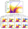 |
Fig. B.1 Same as Fig. 3 but comparing the LMC complete and optimal sample. |
| In the text | |
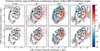 |
Fig. B.2 Same as Fig. 6 but comparing the LMC complete and optimal sample. |
| In the text | |
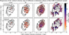 |
Fig. B.3 Same as Fig. 7 but comparing the LMC complete and optimal sample. |
| In the text | |
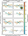 |
Fig. B.4 Same as Fig. 8 but comparing the LMC complete and optimal sample. |
| In the text | |
Current usage metrics show cumulative count of Article Views (full-text article views including HTML views, PDF and ePub downloads, according to the available data) and Abstracts Views on Vision4Press platform.
Data correspond to usage on the plateform after 2015. The current usage metrics is available 48-96 hours after online publication and is updated daily on week days.
Initial download of the metrics may take a while.