| Issue |
A&A
Volume 669, January 2023
|
|
|---|---|---|
| Article Number | A91 | |
| Number of page(s) | 21 | |
| Section | Extragalactic astronomy | |
| DOI | https://doi.org/10.1051/0004-6361/202244601 | |
| Published online | 18 January 2023 | |
Kinematic analysis of the Large Magellanic Cloud using Gaia DR3⋆,⋆⋆
1
Departament de Física Quàntica i Astrofísica (FQA), Universitat de Barcelona (UB), C Martí i Franqués, 1, 08028 Barcelona, Spain
2
Institut de Ciències del Cosmos (ICCUB), Universitat de Barcelona, Martí i Franquès 1, 08028 Barcelona, Spain
e-mail: This email address is being protected from spambots. You need JavaScript enabled to view it.
3
Institut d’Estudis Espacials de Catalunya (IEEC), C Gran Capità, 2-4, 08034 Barcelona, Spain
4
Lund Observatory, Department of Astronomy and Theoretical Physics, Lund University, Box 43 22100 Lund, Sweden
5
Centro de Astronomía – CITEVA, Universidad de Antofagasta, Avenida Angamos 601, Antofagasta 1270300, Chile
6
Departamento de Física de la Tierra y Astrofísica, Facultad de Ciencias Físicas, Plaza de las Ciencias, 1, 08028 Madrid, Spain
7
Instituto de Astronomía, Universidad Nacional Autónoma de México, Apartado Postal 106, 22800 Ensenada, B.C., Mexico
Received:
26
July
2022
Accepted:
1
October
2022
Abstract
Context. The high quality of the Gaia mission data has allowed for studies of the internal kinematics of the Large Magellanic Cloud (LMC) to be undertaken in unprecedented detail, providing insights into the non-axisymmetric structure of its disc. Recent works by the Gaia Collaboration have already made use of the excellent proper motions of Gaia DR2 and Gaia EDR3 for a first analysis of this sort, but these were based on limited strategies aimed at distinguishing the LMC stars from the Milky Way foreground that did not use all the available information. In addition, these studies could not access the third component of the stellar motion, namely, the line-of-sight velocity – which has now become available via Gaia DR3 for a significant number of stars.
Aims. Our aim is twofold: 1) to define and validate an improved, more efficient and adjustable selection strategy to distinguish the LMC stars from the Milky Way foreground; 2) to check the possible biases that assumed parameters or sample contamination from the Milky Way can introduce in analyses of the internal kinematics of the LMC based on Gaia data.
Methods. Our selection was based on a supervised neural network classifier, using as much as of the Gaia DR3 data as possible. Based on this classifier, we selected three samples of candidate LMC stars with different degrees of completeness and purity. We validated these classification results using different test samples and we compared them with the results from the selection strategy used in the Gaia Collaboration papers, based only on the proper motions. We analysed the resulting velocity profiles and maps for the different LMC samples and we checked how these results change when we use the line-of-sight velocities that are available for a subset of stars.
Results. We show that the contamination in the samples from Milky Way stars basically affects the results for the outskirts of the LMC. We also show that the analysis formalism used in absence of line-of-sight velocities does not bias the results for the kinematics in the inner disc. Here, for the first time, we performed a kinematic analysis of the LMC using samples with the full three dimensional (3D) velocity information from Gaia DR3.
Conclusions. The detailed 2D and 3D kinematic analysis of the LMC internal dynamics demonstrate that: 1) the dynamics in the inner disc is mainly bar dominated; 2) the kinematics on the spiral arm overdensity seems to be dominated by an inward motion and a rotation that is faster than that of the disc in the part of the arm attached to the bar; 3) the contamination of Milky Way stars seem to dominate the outer parts of the disc and mainly affects old evolutionary phases; and 4) uncertainties on the assumed disc morphological parameters and line-of-sight velocity of the LMC can (in some cases) have significant effects on the results of the analysis.
Key words: galaxies: kinematics and dynamics / Magellanic Clouds / astrometry
The LMC/MW classification probability of each object is available at the CDS via anonymous ftp to cdsarc.cds.unistra.fr (130.79.128.5) or via https://cdsarc.cds.unistra.fr/viz-bin/cat/J/A+A/669/A91
Movies are available at https://www.aanda.org.
© The Authors 2023
 Open Access article, published by EDP Sciences, under the terms of the Creative Commons Attribution License (https://creativecommons.org/licenses/by/4.0), which permits unrestricted use, distribution, and reproduction in any medium, provided the original work is properly cited.
This article is published in open access under the Subscribe-to-Open model. This email address is being protected from spambots. You need JavaScript enabled to view it. to support open access publication.
1. Introduction
The Large Magellanic Cloud (LMC) is one of the Milky Way (MW) satellite galaxies and a member of the Local Group.
The LMC is the prototype of dwarf, bulgeless spiral galaxy (the so-called Magellanic type: Sm), with an asymmetric stellar bar, many star forming regions, including the Tarentula Nebula, and prominent spiral arms (e.g., Elmegreen & Elmegreen 1980; Gallagher & Hunter 1984; Yozin & Bekki 2014; Gaia Collaboration 2021b). The LMC is a gas-rich galaxy characterised by an inclined disc (e.g., van der Marel & Cioni 2001; van der Marel 2001), with several warps (e.g., Olsen & Salyk 2002; Choi et al. 2018; Ripepi et al. 2022) and an offset bar whose origin is not well understood (e.g., Zaritsky 2004). Due to its proximity, the LMC is a perfect target for many studies and focused photometric surveys, such as VMC-VISTA Survey of the Magellanic Clouds system (Cioni et al. 2011) or SMASH-Survey of the Magellanic Stellar History (Nidever et al. 2017), as well as the astrometric mission Gaia (ESA). Already in Gaia Collaboration (2018; 2021b, hereafter, MC21), the authors show the capabilities of Gaia to characterise the structure and kinematics of this nearby galaxy. The recovery of its three-dimensional (3D) structure using Gaia data only has been shown to be complex due to the zero point in parallax and limit in parallax uncertainties (MC21, Lindegren et al. 2021a,b). Recent attempts using specific populations for which individual distances can be anchored, such as in the populations of Cepheids (Ripepi et al. 2022) or RR Lyrae (Cusano et al. 2021), have been more effective. Three-dimensional structure analysis is not the only tool for inferring the characteristics and morphologies of the galaxy under study. Kinematic profiles and kinematic maps provide additional information on the characteristics and dynamical evolution of the galaxy (Gaia Collaboration 2018; Vasiliev 2018, MC21).
The presence of non-axisymmetric features, such as a bar or spiral arms, modifies the velocity map of a simply rotating disc. The nature of the spiral arms – whether it is a density wave (Lindblad 1960; Lin & Shu 1964), a tidally induced arm (e.g., Toomre & Toomre 1972), transient co-rotating arms (Goldreich & Lynden-Bell 1965; Julian & Toomre 1966; Toomre 1981), or bar induced (e.g., Athanassoula 1980; Romero-Gómez et al. 2007; Salo et al. 2010; Garma-Oehmichen et al. 2021) – can be disentangled from its signature in the velocity field (e.g., Roca-Fàbrega et al. 2013, 2014). The question of how the LMC became so asymmetric, particularly with regard to the ultimate origin of its spiral arm in contrast to more massive spiral galaxies, remains unclear. Thus, detailed kinematic profiles and maps are necessary to supplement its investigation.
Kinematics of stars in the outskirts of the LMC have shed some light on the characteristics of the stellar bridge generated by the tidal interaction between the Large and Small Magellanic Clouds (Zivick et al. 2019; Schmidt et al. 2020), the formation of the LMC’s northern arm (Cullinane et al. 2022a), or the dynamical equilibrium of the disc (Cullinane et al. 2022b). Pre-Gaia proper motions and line-of-sight velocities of less than a thousand stars where used by Kallivayalil et al. (2013), van der Marel & Kallivayalil (2014) to show the detailed large-scale rotation of the LMC disc. The number of sources increased by orders of magnitude when using Gaia DR2 proper motions to study the internal motion of the LMC (Gaia Collaboration 2018; Vasiliev 2018). Wan et al. (2020) used Carbon Stars and Gaia DR2 proper motions to infer the LMC centre, systemic motion, and morphological parameters to compare them with other stellar populations. Similarly, the improved accuracy of Gaia EDR3 (MC21, Niederhofer et al. 2022) allowed for a detailed study of the LMC disc kinematics with the aim of separating the analysis based on different stellar evolutionary phases, in addition to extending the study to the LMC outskirts and bridge between the LMC and SMC.
In this work, we focus on the general kinematic analysis of the LMC disc and we present the first 3D velocity maps and profiles of the LMC measured using Gaia DR3 proper motions and line-of-sight velocities. It is the first time that a homogeneous data set of a galaxy that is not the Milky Way is presented with 3D velocity information, for more than 20 thousand stars. We compare the maps with the ones obtained from previous Gaia releases where only astrometric motions were considered. With the new maps, we want to assess where, and to what extent, the kinematics have benefitted from the line-of-sight velocities.
This paper is organised as follows. In Sect. 2, we describe the LMC samples used throughout this work. We use a new supervised classification strategy based on neural networks to separate the LMC stars from the MW foreground stars. In this section, we also describe the training sample, along with how we applied the classifier to Gaia data and how we validated the classification. In Sect. 3, we describe the formalism adopted to transform from Gaia observables to the LMC reference frame and demonstrate its validation using an N-body simulation. In Sect. 4, we show the detailed kinematic analysis of the LMC samples, showing the velocity profiles and the velocity maps of the different LMC samples. In Sect. 5, we study possible biases on the velocity maps caused by the unknown LMC 3D geometry, as well as uncertainties in the systemic motion. Finally, in Sect. 6, we summarise the main conclusions of this work.
2. Data selection
In this section, we describe the method to select the samples of stars used in this paper. Our starting point is the base sample obtained by selecting Gaia DR3 (Gaia Collaboration 2021a) stars around the center of the LMC. This base sample is a mixture of MW foreground stars and LMC stars. Ideally, it is possible to distinguish both types of objects through their distances, but due to the high uncertainties on the parallax-based distances at LMC (MC21, Lindegren et al. 2021b), a selection of LMC sources exclusively based on parallaxes is not possible and would be efficient only in the process of removing bright MW stars.
Therefore, in order to build a sample of LMC stars for the kinematic analysis in this paper, we need to define a selection criteria to separate them from the MW foreground. A first option is to use a proper motion based selection (Sect. 2.2) as done in MC21; we have kept this methodology to provide a common reference with the results in that paper. We also implemented an alternative selection method based on machine learning classifiers (neural networks, see Sect. 2.3) because, firstly, a selection purely based on proper motions might have some effect on the kinematic analysis and, secondly, we wanted to use the full data available in the Gaia catalogue to improve the classification.
We created the following working samples:
| Based on Gaia data |
| Gaia base sample: initial Gaia DR3 sample selected around the LMC center, before applying any further cut or classification (described in Sect. 2.1) |
| Gaia LMC Proper Motion (PM) sample: application of a proper motion cut to the Gaia base sample (described in Sect. 2.2) |
| LMC complete, optimal, and truncated-optimal samples: resulting from the NN classification (described in Sect. 2.3.3) |
| LMC complete, optimal, and truncated-optimal samples: resulting from the NN classification (described in Sect. 2.3.3) |
Validation samples (described in Sect. 2.3.5):
|
| Based on simulations |
| Gaia (MW+LMC) training sample: simulation based on the Gaia Object Generator (GOG, described in Sect. 2.3.1). |
2.1. Gaia base sample
The Gaia base sample was obtained using a selection from the gaia_source table in Gaia DR3 with a 15° radius around the LMC centre defined as (α, δ) = (81.28°, −69.78° ) (van der Marel 2001) and a limiting G magnitude of 20.5. We only kept the stars with parallax and integrated photometry information, since they are used in the LMC/MW classification. This selection can be reproduced using the following ADQL query in the Gaia archive:
SELECT * FROM gaiadr3.gaia_source as g
WHERE 1=CONTAINS(POINT('ICRS',g.ra,g.dec),
CIRCLE('ICRS',81.28,-69.78,15))
AND g.parallax IS NOT NULL
AND g.phot_g_mean_mag IS NOT NULL
AND g.phot_bp_mean_mag IS NOT NULL
AND g.phot_rp_mean_mag IS NOT NULL
AND g.phot_g_mean_mag < 20.5.
The resulting base sample contains a total of 18 783 272 objects.
2.2. Proper motions-based classification
We use the same selection based on the proper motions of the stars as in MC21 to provide a baseline comparison with these previous results. In short, the median proper motions of the LMC are determined from a sample restricted to its very centre, minimising the foreground contamination by a cut in magnitude and parallax. We kept only stars those whose proper motions obey the constraint of χ2 < 9.21, that is, an estimated 99% confidence region (see details in Sect. 2.2 of MC21). The resulting sample (hereafter, PM selection) contains 10 569 260 objects1.
2.3. Neural network classifier
In order to improve the separation of the MW foreground from the LMC stars, we used classifiers exploiting all the information available in the Gaia DR3 catalogue. Starting from a reference sample where both types of objects are labelled, we trained a classifier that uses the DR3 data to optimize the separation. Then, we applied the trained classifier to our base dataset and checked its performance with several validation subsets. This is an approach already used in other works; for instance, Schmidt et al. (2022) applied a support vector machine classifier trained on a sample where the MW-LMC distinction is based on StarHorse (Anders et al. 2022) distances. However, these authors applied it to data from both Gaia EDR3 and the Visible and Infrared Survey Telescope for Astronomy (VISTA) survey of the Magellanic Clouds system (VMC; Cioni et al. 2011), limiting the number of objects available. Here, we use only Gaia data which allow us to obtain larger samples.
2.3.1. Description of the Gaia training sample
The training sample is a crucial element for the performance of a classifier. It needs to: have the same observational data we use (Gaia DR3) and be as representative of the problem sample as possible, while, at the same time, the classification of its elements should be very reliable. Otherwise, the trained classifier will inherit the problems of the training sample, from biases in the selection to errors in the classification. A first possible approach for building a training sample is to use real data, that is, to use a sub-sample of our base dataset which has an (external) accurate classification of its objects into MW and LMC. We identified two possible options for this approach; on the one hand, we can use samples of RR-Lyrae and Cepheid stars. Since distances for these objects can be accurately determined using period-luminosity relations, they can be located with precision in the LMC and thus distinguished from foreground objects. However, the samples available in this case are rather small and are composed of very specific types of stars. They are not representative of our global samples, which contains stars of all types. On the other hand, we can use the distances in StarHorse EDR3 (Anders et al. 2022) to distinguish MW from LMC objects; however, these distances are based on specific priors for MW/LMC and thus impose some preconditions on the objects, with the risk of propagating these preconditions to our classification. Furthermore, StarHorse only reaches a bright limit G ≤ 18.5 and it therefore does not cover our faint limit of G = 20.5, demonstrating that it is not representative of our problem. For these reasons, we preferred not to use these samples for the training of the classifiers, but we did use them later on as validation samples to check our results, as described in Sect. 2.3.5.
A second possible approach, namely, the one we adopted in this work, is to use representative simulations. A suitable training sample for the classifier would be a simulation based on stellar populations similar to the problem ones and with simulated observations mimicking the Gaia data. As part of the mission preparation, the Gaia Object Generator (GOG; Luri et al. 2014) was developed and has been regularly updated. It produces realistic simulations of the Gaia data and it specifically contains separate modules for the simulation of the MW and the LMC stellar content. We used GOG to produce a training dataset that, like our base sample, corresponds to a simulation of a 15° radius area around the LMC centre, defined as (α, δ) = (81.28° , − 69.78° ), and the LMC simulation has been tailored to make it compatible with recent estimations of the mean distance and systemic motion obtained from EDR3 data: a distance of 49.5 kpc (Pietrzyński et al. 2019) and a systemic motion of μα* = 1.858 mas yr−1, μδ = 0.385 mas yr−1 as in MC21.
This Gaia training dataset is divided in two parts, one for the MW and the other for the LMC. The LMC simulation contains only 277 178 stars, a number that is too small when compared with real data. This is due to the design of the GOG simulator; to provide a realistic spatial distribution of the LMC simulation, it is based on a pre-defined catalogue of OGLE stars, providing real positions (see details in Luri et al. 2014). The MW simulation, on the contrary, is based on a realistic galactic model, and generates a number of stars that matches the observations. This difference would give a too small LMC/MW ratio of objects, and we corrected it by retaining only a random 20% fraction of the MW simulation, resulting in a total of 1 269 705 stars. Furthermore, during the trial-and-error phase of our selection of the configuration for the NN, we found that the classification results for the test samples (taken from the simulation data) were rather insensitive to changes in this ratio, with almost perfect ROC curves. The characteristics of the resulting simulations are summarised in Fig. 1.
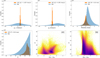 |
Fig. 1. Characteristics of the GOG simulated samples. Top left and middle: distribution of proper motions in right ascension and declination, respectively. In orange and blue: LMC and the MW training samples. Top right: parallax distribution. Bottom left: magnitude G distribution of the simulated samples. Bottom middle and right: colour-magnitude diagram of the LMC and MW, respectively. Colors represent relative stellar density, with darker colors meaning higher densities. |
The merging of these two simulations constitute our training sample, and in Fig. 2, we compare it with the Gaia base sample. These plots show that the Gaia training sample approximately matches the main characteristics of the Gaia base sample, but its limitations are also apparent; the distribution of the LMC stars in the sky forms a kind of square, owing to its origin based on an extraction of the OGLE catalogue; the colour-magnitude diagram (CMD) for the LMC simulation is not fully representative at the faintest magnitudes, with a lack of stars and an artificial cut line; and the distributions of parallaxes and proper motions do not completely match. In spite of these drawbacks, we consider these samples to be sufficiently representative and we go on to check its performance with several validation samples to confirm its suitability.
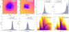 |
Fig. 2. Comparison between the Gaia base and training samples. Top from left to right: density distribution in equatorial coordinates of the Gaia base and Gaia training samples in logarithmic scale, parallax, and G magnitude distributions. Bottom from left to right: proper motion distributions in right ascension and declination and colour-magnitude diagrams for the Gaia base and training samples. In the histograms, in gray we show the Gaia base sample, while in dotted purple we show the Gaia training sample. In the color-magnitude diagrams, colors represent relative stellar density with darker colors meaning higher densities. |
2.3.2. Training the classifier
To implement a classifier, we used the sklearn Python module (Pedregosa et al. 2011). This module contains a variety of classifiers that can be applied to our problem, given the available Gaia data: position (α, δ), parallax and its uncertainty (ϖ, σϖ), along with the proper motions and their uncertainties (μα*, μδ, σμα*, σμδ), and Gaia photometry (G, GBP, GRP). Using the training sample described in the previous section, we trained a classifier to distinguish the MW foreground objects from the LMC objects in our base sample.
In the first stage, we tried a variety of algorithms and evaluated them internally using our simulated dataset: we split it into two parts: 60% for training the algorithm and 40% to test its results. We evaluated its performance by generating the corresponding receiver operating characteristic (ROC) curve and calculating the area under the curve (AUC). The ROC curve is one of the most important evaluation metrics for checking the performance of any classification model. It summarizes the trade-off between the true positive rate and false positive rate using different probability thresholds. The AUC of the ROC curve is another good classifier evaluator. The larger the AUC, the better the classifier works. An excellent model has AUC near to 1 which means it has a good measure of separability. When AUC = 0.5, it means the model has no class separation capacity. From these results, we selected three algorithms that were providing the best results: random forest (RF), K nearest-neighbors (KNN), and a neural network (NN). In all three cases, the ROC curve was almost perfect, similar to that of Fig. 3 corresponding to the NN case.
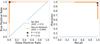 |
Fig. 3. Evaluation metrics for the Neural Network classifier performance. Left: ROC curve. Black dot is in the “elbow” of the ROC curve and it shows the best balance between completeness and purity. The purple star shows the completeness threshold. Right: precision-recall curve. In both cases, we compare our model (orange solid curve) with a classifier that has no class separation capacity (blue dashed curve). |
After testing these three algorithms with the validation datasets described above (RR-Lyrae, Cepheids, and StarHorse) and checking that they retained most of the RR-Lyrae and Cepheids when completeness was prioritised (low probability threshold) we finally selected the NN algorithm. We discarded the KNN because this type of algorithm may be too sensitive to the particularities and representativeness of the training sample (which, as we have seen, is limited). This was indeed the case with our samples, where for instance the square-like shape of the training sample was clearly showing in the classification results for the base sample. We also discarded the RF algorithm because it produced a less sharp MW/LMC distinction. Thus, we ultimately retained the NN classifier.
Focusing on the NN classifier, we tested a few configurations and settled on a NN with 11 input neurons, corresponding to the 11 Gaia parameters listed above; three-hidden-layers with six, three, and two nodes, respectively; and a single output which gives for each object the probability P of being a LMC star (or, conversely, the probability of not being a MW star). A P value close to 1 (0) means that the object is highly likely to be of the LMC (MW). We notice that a wider exploration of NN configurations is possible and we could test selection priorities other than “purity” or “completeness” (see below) in the classification, but we leave this exploration to a future work. We used the rectified linear unit (ReLU) as the activation function. Our model optimizes the log-loss function using stochastic gradient descent with a constant learning rate. The L2 regularization term strength is 1e-52.
In the left panel of Fig. 3, we show the ROC curve of our NN classifier. We obtained an AUC equal to 0.999, which means that our classifier separates with high-precision the LMC and MW stars in the (simulated) test sample. In the right panel of Fig. 3, we show the precision-recall curve. It is another metric that is useful for evaluating the classifier output quality when the classes are very imbalanced. The precision (ratio of true positive vs. total of stars classified as LMC) is a measure of result relevancy, while recall (ratio of true positives vs. total LMC stars) is a measure of how many truly relevant results are returned. As for the ROC curve, it shows the trade-off between precision and recall for different probability thresholds.
A final warning regarding the performance of our NN: both the ROC (AUC) and the precision-recall curve show an almost perfect classifier, but these results correspond to its application to the fraction of our simulated sample used for testing. In the next section, and with the aim to evaluate the performance with real data, we go on to check the NN results when applied to real samples with independent classifications.
2.3.3. Applying the classifier to the Gaia base data
Once the NN is trained, we apply it to the Gaia base sample and obtain probabilities for each of its objects. The resulting probability distribution is shown in Fig. 4. We can notice two clear peaks, one with a probability value near 0 and another with probability value near 1. These peaks correspond to stars that the classifier has clearly identified as MW and LMC, respectively; in between, there is a flat tail of intermediate probabilities.
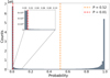 |
Fig. 4. Probability distribution of the Gaia base sample for the NN classifier. A probability value close to 1 (0) means a high probability of being a LMC (MW) star. |
To obtain a classification using the probabilities generated by the classifier for each star, we need to fix a probability threshold Pcut. If P > Pcut, the star is considered to belong to the LMC; if P < Pcut, the star is considered to belong to the MW (alternatively, we could leave stars with intermediate probabilities as unclassified). By fixing a low probability threshold we seek not to miss any LMC object, and the resulting LMC-classified sample to be more complete at the price of including more “mistaken” MW stars. On the contrary, by fixing a high probability threshold, we can make the resulting LMC-classified sample to be purer (less mistakes), at the price of missing some LMC stars and thus obtaining a less complete sample.
The purity-completeness trade-off is a decision that will define the properties of the resulting sample and therefore can have an effect on the results obtained from it. In this work, we define three different samples to explore the effects of this trade-off:
1. Complete sample (Pcut = 0.01). In this case a cut at small probabilities prioritizes completeness, making sure that no LMC objects are missed at the prize of an increased MW contamination. The cut value was chosen by inspecting the probability histogram of the classification (Fig. 4) and selecting the limit of the main peak of small probability values.
2. Optimal sample (Pcut = 0.52). In this case the probability cut was chosen to be optimal in a classification sense; the value corresponds to the “elbow” of the ROC curve (Fig. 3), which is in principle the best balance between completeness and purity.
3. Truncated-optimal sample (Pcut = 0.52), plus an additional cut for G > 19.5 mag.
We introduced the third case because, after examining the results for the optimal sample, we noticed that the faint tail of its magnitude distribution most likely corresponds to MW stars; MW stars exponentially increase at fainter magnitudes, while LMC stars quickly decrease after G ≃ 19.5 (see discussion in the next section). Furthermore, with this cut we manage to avoid a region in the faint end where the LMC training sample is not representative, as discussed above; removing these stars can reduce the MW contamination (see Sect. 2.3.5) and also discards the stars with larger uncertainties and, therefore, less useful for our kinematic analysis. A further selection could be made by excluding regions of the CMD diagram where contamination is more likely, but given the cleanliness of the LMC diagrams in Fig. 6 we deemed this not necessary.
Finally, for each of the four samples we consider two datasets. First, the full sample where we assume that all the stars have no line-of-sight velocity information. Second, a sub-sample of the first one where we only keep stars with Gaia DR3 line-of-sight velocities. We refer to these sub-samples as the corresponding Vlos sub-samples. The number of stars per dataset is in the second and third column of Table 1, respectively, together with the mean astrometric information.
Comparison of the LMC samples number of sources and mean astrometry between the proper motion selection (MC21) and the neural networks.
2.3.4. Comparison of classifications
The sky density distributions for the classified LMC/MW members in our different samples are shown in Fig. 5. In the left column, we show the LMC selection in each of the samples, while in the right column, we show the sources classified as MW. Each row corresponds to one selection strategy: proper motion selection (first row) followed by the three NN based ones. As expected, the results of the proper motion based selection are very similar to that described in MC21.
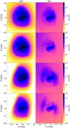 |
Fig. 5. Sky density distribution in equatorial coordinates of both the LMC (left) and MW (right) sample obtained from the different classifiers. First row: proper motion selection classification. Second row: Complete NN classification. Third row: optimal NN classification. Fourth row: truncated-optimal NN classification. Note: in the fourth row, we display a cut in magnitude G > 19.5 for both the LMC and MW samples and, therefore, the total number of stars is reduced. |
We note here that the limited spatial distribution of the LMC training sample (square region in top-left panel of Fig. 2) does not pose a problem for extrapolating the membership beyond this region, since an anomalous classification in the LMC outskirts is not observed in these figures. In order to evaluate the extrapolation performance, we also tested the NN classifier when not taking into account the positional information; the results show that even in this extreme case the classifier does not have problems with the spatial distribution of the resulting samples.
We also note that sources classified as belonging to the MW by all four samples show an overdensity in the most crowded region of the LMC, that is, the bar, indicating misclassifications of LMC stars. We also see that, as expected by the definition of the probability cut, the more complete the LMC sample, the less stars are classified as belonging to the MW. In this respect, a cross-matching of the proper motion selection sample and the complete sample shows that the second almost completely contains the former: of the 10 569 260 stars of the Proper motion sample, 10 432 704 of them are included in the complete sample and the complete sample contains almost two million additional stars.
In Table 1 we also see that the dispersion of the astrometric parameters diminish from the NN complete to the NN truncated-optimal samples. This is expected, since the stricter sequence of selection criteria lead to a higher similarity in distance and velocity inside the samples.
In Fig. 6, we compare the astrometry and photometry distribution of the different LMC samples. In the proper motion selection sample, we see that the sharp cut in proper motion imposed makes the distribution of proper motion to be narrow around the bulk motion of the LMC, while in the MW classification, two small peaks are present, following a continuation of the LMC peak. Clearly, some LMC stars are misclassified as MW using the sharp cut in proper motion. This misclassification is not visible in the NN complete sample and is present again in the more restrictive optimal and truncated-optimal samples. The parallax distribution in the four LMC samples are very similar, with the truncated optimal sample being the most narrow. The G magnitude distributions are quite different in the four LMC selections. Both the PM and the NN samples show a peak in G magnitude around G ∼ 19 mag, which corresponds to the LMC sample, and a secondary peak at the limiting magnitude of G = 20.5, corresponding to MW contamination. For this reason, as described above, we define the truncated-optimal sample by removing the secondary peak in the optimal sample. Conversely, the MW selection in all cases should show an exponential distribution in G, though the PM, the complete and the optimal samples show a secondary peak of varying significance amongst them around G ∼ 19 mag. The CMD of all LMC samples is very similar. Small differences only appear in the MW selection of the optimal and truncated optimal sample which contain, as expected, sources of the red giant branch of the LMC, which the NN classifier misclassifies as MW.
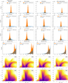 |
Fig. 6. Astrometric and photometric characteristics of the LMC and MW samples. From left to right: PM sample, NN complete, NN optimal and NN truncated-optimal samples. In the first four rows, we show distributions of proper motion in right ascension and declination, parallax, and G magnitude, respectively, of the LMC (orange) and MW (blue) samples. In the last two rows, we show the colour-magnitude diagram of the samples classified as LMC and MW, respectively. Color represents the relative stellar density, with darker colors meaning higher densities. |
2.3.5. External validation of the classification
As indicated in previous sections, to validate the results of our selection criteria we compare them with external independent classifications. To do so, we cross-matched our base sample with three external samples:
– LMC Cepheids (Ripepi et al. 2022): we used the paper’s sample of 4500 Cepheids as a set of high-reliability LMC objects. To obtain the Gaia DR3 data we cross-matched the positions given in the paper with the Gaia DR3 catalogue, using a 0.3″ search radius to obtain high confidence matches, thus retaining 4485 stars. Finally, we introduced a cut of 15° radius around the LMC center (mimicking our base sample), leading to a final selection of 4467 LMC Cepheids.
– LMC RR-Lyrae (Cusano et al. 2021): similarly to the process above, we used the paper’s sample of 22 088 RR-Lyrae as high-reliability LMC objects. After the cross-match with the Gaia DR3 catalogue, the sample is reduced down to 22 006 stars and after the in 15° radius cut around the LMC center we obtain a final sample of 21 271 LMC RR-Lyrae.
– StarHorse (Anders et al. 2022): we cross-matched this catalogue with the Gaia DR3 data using a cut of 15° radius around the LMC center and obtained a sample of 3 925 455 stars. Following a similar criteria to the one proposed in Schmidt et al. (2020, 2022), we separated MW and LMC stars through the StarHorse distances, but making a cut at d = 40 kpc. This decision is motivated by the distance distribution of the StarHorse sample, which is shown in Fig. 7. A cut in d = 40 kpc gives a very restrictive classification, minimizing the contamination of MW stars (see discussion below). We thus obtain a StarHorse LMC sample with 985 173 stars and a StarHorse MW sample with 2 940 282 stars. Notice that being based on StarHorse, this sample contains stars only up to G = 18.5.
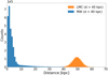 |
Fig. 7. Distance distribution of the StarHorse validation sample. In blue (orange), the StarHorse stars classified as MW (LMC) according to the d = 40 kpc criteria. |
The Cepheids and RR-Lyrae samples contain objects classified with high reliability as LMC stars, so they serve as a check of the completeness of our classification for LMC objects (“how many we lose”). On the other hand, the StarHorse sample is helpful to estimate the contamination caused by wrongly classified MW stars, although this can only be taken as an indication, since the StarHorse classification itself is not perfect. Furthermore, given the very stringent criteria used for the separation in StarHorse (the cut in d = 40 kpc), the resulting estimation of MW contamination in the classification will be a “worst case”.
In Table 2, we summarize the comparison of the results of our four classification criteria applied to stars contained in the three validation samples. It can be seen that the completeness of the resulting LMC classifications is quite good, usually above 85%, as shown for the results with the Cepheids, RR-Lyrae and StarHorse LMC validation samples. The exception is the truncated-optimal sample, where the completeness is reduced for the RR-Lyrae, due to the cut in faint stars.
Matches of the classified LMC members in our four considered samples against the validation samples.
On the other hand, the relative contamination by MW stars in the samples is more difficult to assess. We have to rely on the StarHorse distance-based classification as an external comparison, with the caveat that this classification contains its own classification errors. To do so, we re-calculate the precision-recall curve, but this time taking the StarHorse classification as a reference; the result is shown in Fig. 8. We can see that the precision remains quite flat for almost all the range of the plot, that is, for all the range of probability threshold values. This indicates that the relative contamination (percentage of stars in the samples that are MW stars wrongly classified as LMC stars) is similar in the complete and optimal samples (the more restrictive we are, the more MW stars we remove, but also we lose more LMC stars). Taking the precision values in Fig. 8 indicates that in using the classification based on SH distances as a reference, the relative contamination of our samples could be around 40%; this is a worst case, since we used a very restrictive distance cut (40 kpc) and when using less restrictive cuts (down to 10 kpc), the estimation of the contamination can be lowered to ∼30%. These numbers have to be taken with care, since the MW-LMC separation based on the SH distances is not perfect, just another possible classification criteria that in fact is using less information than our criteria. As pointed in the SH paper (Anders et al. 2022), these populations are clearly visible as overdensities in the maps, although a considerable amount of stars still has median distances that fall in between the Magellanic Clouds and the MW – a result of the multimodal posterior distance distributions.
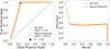 |
Fig. 8. Evaluation metrics for the Neural Network classifier performance using the StarHorse sample. Left: ROC curve. Black dot is in the “elbow” of the ROC curve and it shows the best balance between completeness and purity. Right: precision-recall curve. In both cases, we compare our model (orange solid curve) with a classifier that has no class separation capacity (blue dashed curve). |
These results point out to a possible contamination by MW stars in our samples around some tens of percentage but we can do an additional check using the line-of-sight velocities in Gaia DR3, which are available only for a (small) subset of the total sample. These line-of-sight velocities are not used by any of our classification criteria and have different mean values for the MW and LMC (therefore providing an independent check). In Fig. 9, we plot the histograms of line-of-sight velocities separately for stars classified as MW and LMC, and it is clear from these that the contamination of the LMC sample is reduced, likely to be significantly below the levels suggested above. For instance, if we consider the LMC NN complete sample and (roughly) separate the MW stars with a cut at Vlos < 125km s−1, we estimate the MW contamination to be around 5%. However, since the subset of Gaia DR3 stars with measured line-of-sight velocities contains only stars at the bright end of the sample (G ≲ 16), this check is not fully representative either.
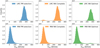 |
Fig. 9. Line-of-sight velocity distribution for the stars classified as LMC (top) and MW (bottom). We show the three Vlos sub-samples of the PM selection (left), NN complete (middle) and NN optimal (right) samples. |
Finally, we made a new query to the Gaia archive that was similar to that defined in Sect. 2.1. This time, we made a selection from the gaia_source table in Gaia DR3 with a 15° radius in a nearby region with homogeneous sky density. This way we can make an estimation of the MW stars expected in a regions similar to that covered by our Gaia base sample. From this new query, we obtained 4 240 771 stars, so we would expect a similar number of MW stars in the region we selected around the LMC. Given that the Gaia base sample contains 18 783 272 objects and the number of objects classified as LMC (Table 1) is around 6 − 12 million, the number of stars classified as MW is around 12 − 6 million; therefore, we can conclude that our NN LMC samples prioritise purity over completeness since there are too many stars classified as MW (an excess of 2–8 million). This is also evident from the right panels of Fig. 5, where the distribution of stars classified as MW shows the pattern of LMC contamination.
3. Coordinate transformations and validation
3.1. Coordinate transformations
Since the main goal of this work is to look at the internal kinematics of the LMC, we review the coordinate transformations used to compute the LMC-centric velocities. To do so, we revisit the formalism introduced in van der Marel & Cioni (2001) and van der Marel et al. (2002) and describe the two-step process used to transform the Gaia heliocentric measurements to the LMC reference frame (full details are given in Appendix A).
First, we introduce a Cartesian coordinate system (x, y, z), whose origin, O, is placed at (α0, δ0, D0), the LMC centre. The orientation of the x-axis is anti-parallel to the right ascension axis, the y-axis parallel to the declination axis, and the z-axis towards the observer. This is somehow similar to considering the orthographic projection – a method of representing 3D objects where the object is viewed along parallel lines that are perpendicular to the plane of the drawing – of the usual celestial coordinates and proper motions (see Fig. 10 for a schematic view of the observer-galaxy system). We refer to this reference frame as the orthographic projection centred at the LMC.
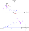 |
Fig. 10. Schematic view of the observer-galaxy system. The LMC center O(α0, δ0, D0) is chosen to be the origin O of the (x, y, z) coordinate system. Top: projected view of the sky. All vectors and angles lie in the plane of the paper. The angles ρ and ϕ define the projected position on the sky of a given point with coordinates (α, δ). Bottom: side view of the observer-galaxy system. The distance from the observer to the LMC center is D0 and the distance from the observer to an object is D. The component v1 lies along the line-of-sight and points away from the observer. |
Second, we transform from the (x, y, z) frame to the final Cartesian coordinate system whose reference plane is the LMC plane, (x′,y′,z′). It consists of the superposition of a counterclockwise rotation around the z-axis by an angle θ, followed by a clockwise rotation around the new x′-axis by an angle i. With this definition, the (x′,y′) plane is inclined with respect to the sky tangent plane by an angle i. Face-on (face-off) viewing corresponds to i = 0° (i = 90°). The angle θ is the position angle of the line-of-nodes or, in other words, the intersection of the (x′,y′)-plane and the (x, y)-plane of the sky. By definition, it is measured counterclockwise from the x-axis. In practice, i and θ will be chosen such that the (x′,y′)-plane coincides with the plane of the LMC disk. Therefore, we refer to this final reference frame as the LMC in-plane reference system.
Since we do not have reliable information for individual distances because the parallaxes are very small and close to the noise (MC21, Lindegren et al. 2021b), we assume that all the stars lie on the LMC disc plane, as an approximation. Thus, we impose z′ to be zero, which leads to a distance of Dz′ = 0 (different to the real one) for each star. In Fig. 11, we show a schematic representation of what this assumption implies. We represent the position of a real star in dark gray, while the white star in red solid line is the projection of the real star on the LMC plane. With this strategy all LMC stars are assumed to lie on its plane.
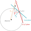 |
Fig. 11. Schematic representation of the reference frames used, all of them centred on the LMC centre (α0, δ0). In blue, we show the orthographic reference frame, (x, y, z), whereas in red, we show the Cartesian LMC frame, (x′,y′,z′). We also show the position of a real star (solid dark gray), its projection in the LMC cartesian frame under the imposition of z′ = 0 (red frame). |
When these two rotations are applied and the stars are made to lie in the LMC plane; for each star, we have LMC-centric positions (x′,y′,0) and velocities (vx′, vy′, vz′). The last step is to make these velocities internal by removing the LMC systemic motion (see details in Appendix A.2.1). In this work (as in MC21), we consider the following LMC parameters: i = 34°, θ = 220°, (α0, δ0) = (81.28° , − 69.78° ), and (μx, 0, μy, 0, μz, 0) = ( − 1.858, 0.385, −1.115) mas yr−1, where we take into account that our x and z-axes have the opposite sense from the one considered in MC21. These values are derived assuming a specific centre, the same one as we use in this work. The distance to the LMC centre is assumed to be D0 = 49.5 kpc (Pietrzyński et al. 2019).
As shown in Eq. (A.8), the formalism presented in van der Marel & Cioni (2001) and van der Marel et al. (2002) allows taking into account line-of-sight velocities, which is something that could not be done when using MC21 transformations. As detailed in Sect. 2.3.3, in this work we deal with two different datasets: the full samples, without line-of-sight velocity information and the sub-samples of stars with individual line-of-sight velocities. For the former, we estimate each star line-of-sight velocity by taking into account its position and proper motion and the global parameters of the LMC plane (full details in Appendix A.3).
In the top panel of Fig. 12, we show the LMC density map for the NN complete sample in the LMC cartesian coordinate system. The density maps for the rest of the three samples are analogous and show the same morphological features as in the corresponding sample of the left column of Fig. 5. Here, we want to point out that the coordinate transformation from the heliocentric equatorial system to the LMC cartesian system inverts the vertical axis, so now the spiral arm starts at negative x′ and y′, and the deprojection of the inclination angle in the sky makes the galaxy elongated along the vertical axis.
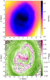 |
Fig. 12. Comparison between density and overdensity maps. Top: LMC density map for the NN complete sample. Bottom: LMC overdensity map for a 0.4 kpc-bandwidth KDE. A black line splitting the overdensities from the underdensities is plotted. Both maps are shown in the (x′,y′) Cartesian coordinate system. |
3.2. Validation of the formalism with a N-body simulation
In this section, we use N-body simulations to test the new formalism introduced above. We use the “B5” isolated barred galaxy simulation of Roca-Fàbrega et al. (2013), which consists of a live disc of 5 million particles and a Toomre parameter of Q = 1.2, and a live NFW halo. The disc to halo mass ratio is the appropriate so that the simulation develops a strong bar and two spiral arms which are transient in time. The snapshot used in this analysis corresponds to an evolution time of T ≃ 500 Myr, and the density distribution is shown in the top left panel of Fig. 13. Using the 6D information of positions and velocities at this given time, we carry out the following exercise. First, we convert the galactocentric cartesian coordinates to heliocentric equatorial (α, δ, d, μα*, μδ, Vlos) at the line of sight, spatial orientation, distance, and systemic motion of the LMC. Then, we consider these particles as a data set and we apply the same formalism described in Sect. 3 to compute the coordinates in the LMC frame and the velocities in cylindrical coordinates. The radial component (left panels) indicates the motion towards as well as away from the galactic centre, while the residual tangential velocity (middle panels) is obtained by subtracting the tangential velocity curve to the tangential velocity component, indicating the motion with respect to the tangential curve. The vertical component (right panels) indicates the motion across the galactic plane.
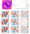 |
Fig. 13. Simulation B5. First row left panel: density distribution in logarithmic scale. First row, right panel: velocity profiles of the B5 simulation. In blue, orange and green, for the radial, tangential, and vertical components, respectively, when taking into account the full velocity information (dashed lines), or when Vlos is not available (solid lines). Differences are negligible and both curves overlap. Scatter points show the real velocity profiles. Second row: N-body simulation maps (left, radial; middle, residual tangential; right, vertical), without applying any coordinate transformation. Third row: same as above computed applying the (Sect. 3) coordinate transformations without line-of-sight information. Fourth row: same as above computed applying the (Sect. 3) coordinate transformations with line-of-sight information. The black line shows the contour corresponding to overdensity equal to zero for a 0.4 kpc-bandwidth KDE (see details in Sect. 4.2). |
We applied the coordinate transformations twice. In the first case, we imposed, as in the LMC full samples, that Vlos is not available and use the internally derived from Eq. (A.15). Secondly, we used the available Vlos, as in the sub-samples, from the 3D velocity data. We computed the velocity profiles and velocity maps with the simulation data as follows. The same procedure is performed when applying it to the LMC samples in Sect. 4. Each curve is obtained by computing the median value of all stars located in radial bins of 0.5 kpc-width in the (x′,y′)-plane. The error in each bin is computed as the division between the median absolute deviation and the square root of the number of stars. The resulting velocity profiles are shown in the top right panel of Fig. 13. The velocity maps are obtained by plotting the median in 100 × 100 bins in the (x′,y′)-plane from −8 kpc to 8 kpc. The resulting velocity maps are shown in the second to fourth row panels of Fig. 13. In the second row, we show the radial, residual tangential, and vertical velocity maps obtained directly from the N-body simulation. In the third and fourth rows, we show the velocity maps when Vlos is not available and when it is, respectively.
From the velocity profiles and maps, we note that the approximation used, when Vlos is not available, does not modify the velocity profiles as seen in the top right panel of Fig. 13, nor the radial and residual tangential velocity maps (see left and middle panels of Fig. 13). The only effect is in the vertical component in the case where Vlos is not available; so, in this case, we obtain  km s−1, which is a consequence of the fact that the internal line-of-sight velocity is estimated by computing the derivative of the distance as function of time (see Eq. (A.15)), which makes
  become null when substituting into the analogous Eq. (A.8) for the internal motion. In the other two cases, namely, when we use the input data or the derived
  from the Vlos, we obtain a median profile and median velocity map centered at zero within the Poisson noise. In the radial and residual tangential velocity component (left and middle panels), we clearly see the quadrupole effect due to the presence of a rotating bar. As expected, the change in sign in VR occurs along the major and minor axes of the bar and the residual tangential velocity is minimum along the bar major axis. Also, we successfully validated the coordinate transformation formalism by artificially inflating the vertical component ten times larger than that of the original B5 simulation to make the radial, tangential, and vertical velocity components comparable in range.
In conclusion, the formalism used to derive the velocities in the LMC frame, when the line-of-sight velocity is not available, does not introduce any bias in the velocity profiles or maps. The most important assumption in the formalism is that all stars lie on a plane.
4. Analysis of the velocity profile and maps
In this section, we analyse the velocity profiles (Sect. 4.1) and velocity maps (Sect. 4.3) for the four samples, and their corresponding Vlos sub-samples (described in Sect. 2). To allow for a comparison between density and kinematics, we overplot the overdensity contour in the velocity maps, as described in Sect. 4.2.
4.1. LMC velocity profiles
Here, we analyse the velocity profiles in the LMC coordinate system. We computed the LMC velocity profiles by using a similar methodology to that used in MC21 (as specified in Sect. 3.2).
In the left panels of Fig. 14, we show the velocity profiles (radial, tangential, and vertical – from top to bottom) for each of the four full LMC samples. In all samples, the radial velocity profile slightly decreases with radius up to 2.5 kpc, where it increases again. The tangential velocity profile shows the rotation curve of the galaxy, having a linear growth until R ∼ 4 kpc in all samples and becoming flat in the outer disc. The maximum tangential velocity varies between LMC samples, with a maximum difference of ∼15 km s−1 at R = 4.7 kpc between the NN complete and NN optimal samples. We use these rotation curves to derive residual tangential velocity maps in Sect. 4.3. The vertical velocity profile for the four samples is completely flat and centered at 0 km s−1, which is a consequence of not using the observational Vlos in these samples, as mentioned in Sect. 3.2. As noted above, the internal line-of-sight velocity is estimated by computing the derivative of the distance as function of time (see Eq. (A.15)), which makes  become null when substituting into the analogous Eq. (A.8) for the internal motion, so we will not use it in the following analysis.
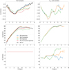 |
Fig. 14. Velocity profiles for the four LMC samples in the case Vlos is not available (left) and when it is available (right). From top to bottom: radial, tangential, and vertical velocity profiles. Each curve corresponds to one LMC sample: PM selection (blue), NN complete (orange), NN optimal (green) and NN truncated-optimal (red). In black, the radial and rotation curve published in MC21 (their Fig. 14) is shown. For most of the bins, the error bar is small and cannot be seen. Only bins with more than 300 sources are plotted. |
We can summarise the comparison between the samples in the following points:
– The PM sample profiles are almost the same as the MC21 for the radial and tangential velocity curves.
– The NN complete sample profiles are very similar to the ones of the PM selection, as also seen in the density maps (see Sect. 2.3.4), with a maximum difference of ∼2 km s−1 at R ≳ 4.5 kpc in the radial component.
– The NN optimal and NN truncated-optimal samples, while they are indeed purer, also have larger inward-streaming motion and rotate about ∼10 − 15 km s−1 more slowly than the more complete samples in the outer disc.
In the right panels of Fig. 14, we show the same velocity profiles, this time with the sub-samples that have full 3D velocity components, this is, with Vlos. The trends observed in the left panels for the radial and tangential profiles are reproduced in the right panels. We note that the radial velocity profile of the Vlos sub-samples has a larger negative amplitude at R = 2 − 3 kpc, of around  km s−1, compared to the
  km s−1 of the full samples. Also, the tangential velocity for the NN sub-samples is now a bit larger and they are all centered around
  km s−1. The largest difference between the main samples and the Vlos sub-samples arises in the vertical velocity component, where we observe different trends between sub-samples:
– The NN truncated optimal sample provides the same profile as the NN optimal sample. This is expected since, in this case, both sub-samples are the same because line-of-sight velocities are available up to G magnitude < 16, and the truncation is performed at G = 19.5.
– All sub-samples have a slightly negative vertical velocity profile. The PM sample is the one that has a flatter profile, centered around −3 km s−1 up to ∼5 kpc. The NN complete sample has an increasing trend from −4 km s−1 to positive values at R = 6 kpc and NN optimal presents a wave-like pattern having a change of sign at R ∼ 4 kpc. These trends are very sensitive to the imposed μz, 0. A small shift to the vertical component of the systemic motion will translate into a shift in the  profile, while differences between sub-samples arise from contamination from the MW, mostly present in the outer disc (see discussion in Sect. 5).
4.2. Determination of the LMC overdensity maps
In this section, we introduce and describe the mask used to highlight the LMC overdensities, such as the bar and the spiral arm.
To analyse the data, we considered 100 × 100 bins in the (x′,y′)-plane of range −8 kpc to 8 kpc, as when constructing the velocity maps. Then, a Gaussian kernel density estimation (KDE) of 0.4 kpc-bandwidth is applied. To highlight the star overdensities, we compute for each bin N/NKDE − 1, where N and NKDE are the number of stars corresponding to the data histogram and the KDE, respectively. The mask N/NKDE − 1 has positive (negative) values for overdensities (underdensities). The value of NKDE is computed by integrating the KDE for the bin area. The choice of the KDE bandwidth was empirical. We built overdensity maps for bandwidths ranging from 0.2 − 1 kpc and we considered that a 0.4 kpc-bandwidth fulfills our objective of highlighting both the LMC bar and arm.
In the bottom panel of Fig. 12, we show the LMC overdensity map in the (x′,y′) Cartesian coordinate system. We can clearly see how both the LMC bar and spiral arm stand out as overdensities, as shown by the black contour of overdensity equal to zero. We first observe how the LMC spiral arm starts at the end of the bar around ( − 3, 0) kpc. Then, if we analyse the spiral arm following a counter-clockwise direction, the spiral arm breaks into two parts: an inner and an outer arm. Finally, both parts join further on and continue together until the spiral arm ends, performing close to a full rotation around the LMC centre.
4.3. LMC velocity maps
In this section, we analyse the velocity maps in the LMC coordinate system for the four LMC samples. The results are shown in Figs. 15–17 for the radial, tangential, and vertical components, respectively. Results are shown from top to bottom for PM selection, NN complete, NN optimal and NN truncated optimal samples, respectively, while left (right) panels show the velocity maps for the full (Vlos sub-) samples. The black line shows the overdensity contour corresponding the overdensity equals to zero (as in the bottom panel of Fig. 12), which helps in making the comparison between density and kinematics.
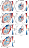 |
Fig. 15. LMC median radial velocity maps. All maps are shown in the (x′,y′) Cartesian coordinate system. From top to bottom: PM sample, NN complete, NN optimal, and NN truncated-optimal sample. Left: line-of-sight velocity not included. Right: line of sight velocity included. NN truncated-optimal Vlos sub-sample map is not shown because it is the same as the NN optimal Vlos sub-sample (see text for details). For each colormap, a black line splitting the overdensities from the underdensities for a 0.4 kpc-bandwidth KDE is plotted and a minimum number of 3 (20) stars per bin is imposed when the line-of-sight is (not) considered. |
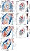 |
Fig. 16. LMC median residual tangential velocity maps. All maps are shown in the (x′,y′) Cartesian coordinate system. From top to bottom: PM sample, NN complete, NN optimal, and NN truncated-optimal sample. Left: line-of-sight velocity not included. Right: line-of-sight velocity included. NN truncated-optimal Vlos sub-sample map is not shown because it is the same as the NN optimal Vlos sub-sample (see text for details). For each colormap, a black line splitting the overdensities from the underdensities for a 0.4kpc-bandwidth KDE is plotted and a minimum number of 3 (20) stars per bin is imposed when the line-of-sight is (not) considered. |
Regarding the radial velocity maps (Fig. 15), the quadrupole pattern already reported in MC21 related to the motion of stars in the bar is present for all samples; however, for Vlos sub-samples, an asymmetry clearly becomes apparent along the semi-major axis of the bar, shown by the change in sign of the radial velocity. We estimate the bar major axis is inclined with respect to the x′-axis about ∼ − 10°. The radial velocities in the upper half of the semi-major axis have larger values (in absolute value) than those on the bottom half. Further research is required to analyse whether this asymmetry is an effect of the inclination of the bar with respect to the galactic plane or whether it is an artifact of the assumption that all stars lie in the plane; although this latter assumption is also present in the full sample, where the asymmetry is also present but less clear. The trend in the outer disc is similar in all full samples, though a strong inward or outward motion in the outskirts of the sample is present in the NN optimal and NN truncated-optimal samples. In particular, the strong inward motion detected in the upper periphery of the NN optimal and NN truncated samples is coherent with the region where the Magellanic Bridge connects to the LMC, and this could represent in-falling stellar content from the SMC. Along the LMC spiral arm, there is a negative (inward) motion along the spiral arm overdensity when this is still attached to the bar, regardless of the sample and the number of velocity components used (left panels of Fig. 15). After the break, there is no a clear trend. In the right panels, the Vlos sub-samples do not have enough number of stars on the spiral arms to provide a clear conclusion.
Regarding the residual tangential velocity maps (Fig. 16), the conclusions with regard to the bar region are analogous to those related to the radial velocity maps, namely, the quadrupole pattern expected for the motion of the stars in elliptical bar orbits is present. The asymmetry in terms of larger velocity in absolute value above the bar major axis is clear in both the full samples and the Vlos sub-samples. This asymmetry in the velocity seems slightly larger in the NN optimal and NN truncated-optimal samples, with a maximum difference of 10 km s−1. Along the spiral arm the residual tangential velocity is in general positive in all samples, that is, stars on the spiral arm move faster than the mean motion at the same radius, except for the part of the arm with a density break. When making comparisons among samples, this aspect represents the effect of the contamination of MW stars in the velocity maps and we can see the decrease of the residual tangential velocity in the edges of the sample in the NN optimal and truncated-optimal samples, which could be a bias of the sample. Regarding the Vlos sub-samples (right panels of Fig. 16), there is no clear sign of the residual tangential velocity along the part of the spiral arm attached to the bar.
Finally, we show in Fig. 17 the vertical velocity component for the Vlos sub-samples. We see, as in the vertical velocity profile, that the vertical velocity map has second order differences between the different samples. More complete samples, such as PM and NN complete samples show a bimodal trend, where half of the galaxy (x′< 0) is moving upwards, while the other half (x′> 0) is moving downwards. There also seems to be a positive gradient (in absolute value) of increasing vertical velocities from the inner to the outer disc. This could be associated with an overestimation of the disc inclination angle or to the presence of a galactic warp (e.g., Choi et al. 2018), or to the contamination of MW stars. Purer samples, such as the NN optimal or NN truncated-optimal still show a similar wave-like motion that can be associated to the warp or to the fact that the LMC is still not in dynamical equilibrium (e.g., Choi et al. 2022). Also, there seems to be a clear negative motion of stars located at the end of the bar with x′> 0, which could be an evidence of the inclination of the bar with respect to the galactic plane.
5. Biases and different evolutionary phases
Velocity maps may be affected by the choice of the galaxy parameters, namely, the inclination, i, and position angle, θ, or the systemic motion, (μx, 0, μy, 0, μz, 0). There remains a large uncertainty in the literature on what the inclination angle of the galactic plane with respect to the line-of-sight and the line-of-nodes of the position angle are, with differences as large as 10° (e.g., van der Marel & Kallivayalil 2014; Haschke et al. 2012; Ripepi et al. 2022). In this work, we use i = 34° and θ = 220°, as nominal values, as in MC21 work. In order to study the possible systematic that a different inclination angle or position angle can induce in the velocity maps, we reproduce the velocity maps for the NN complete sample and corresponding Vlos sub-sample, by varying the nominal values by ±10°, only one at a time. In general, the effect of having a larger (smaller) inclination angle, elongates (stretches) the velocity map, in either of the velocity components, and a different position angle, rotates the velocity maps. In detail, they also introduce the following trends:
Regarding the inclination angle: i) The variation of the inclination angle from i − 10° to i + 10°, can reverse the radial motion in the outer disc from being positive to negative along the y′-axis. ii) The median vertical component can even change sign and become negative if using a smaller inclination angle; whereas when this is 10° larger, a clear bi-symmetry is introduced. iii) The inner disc is not affected, nor the residual tangential component. Regarding the position angle, systematics are of second order and mainly affect the azimuthal angle in the disc where the motion is inwards or outwards and upwards or downwards.
The choice of the systemic motion (μx, 0, μy, 0, μz, 0) used to compute the internal velocities in the LMC reference frame may also introduce systematics in the velocity profile and maps. In this work, we adopted the same systemic motion as in MC21 to allow a direct comparison. The availability of line-of-sight velocities in Gaia DR3 allows a better estimation of μz, 0. For each Vlos sub-sample, we fit a Kernel density estimation of 2 km s−1 bandwidth to the distribution of line-of-sight velocities (see top panels of Fig. 9) and obtain at which line-of-sight velocity this distribution is maximum Vlos, 0. We assume, then, that the line-of-sight systemic motion, μz, 0 of the LMC is given by μz, 0 = Vlos, 0/D0. Results are shown in Table 3, where we show for each sub-sample Vlos, 0 and the corresponding μz, 0. We note that for the PM and NN complete samples μz,0 = − 1.112 mas yr−1 and similar to the value adopted in this work, which is −1.115 mas yr−1. As discussed previously, NN complete sample and PM sample have a very similar LMC classification and thus provide similar density and kinematic distributions. On the other hand, the line-of-sight systemic motion for the NN optimal sample gives μz,0 = − 1.132 mas yr−1, which can provide a different velocity profile in the vertical in-plane component, while it barely has no effect on the planar components. In Fig. 18, we show the vertical velocity profile for each of the three sub-samples when we use either the MC21 adopted value for μz, 0 (dashed lines) or the derived using the Gaia DR3 line-of-sight velocities (solid lines). We note that a bias in the μz, 0 translates in a shift in the  profile. The small difference between the PM and NN complete samples with respect to the MC21 value falls within the error bars. For the NN optimal sample, the currently derived value shifts the median vertical velocity to be centered at zero in the inner 3 kpc, while it is slightly oscillating towards positive values in the outer disc.
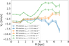 |
Fig. 18. Stellar vertical velocity profiles of the LMC Vlos sub-samples (blue, orange and green for the PM, NN complete, and NN optimal samples, respectively) for different input values of μz, 0: the Gaia DR3 derived in solid lines and the MC21 adopted value in dashed lines (values given in the legend). |
Determination of the line-of-sight systemic motion.
Regarding the tangential systemic motion, (μx, 0, μy, 0), van der Marel et al. (2002) determined (μx, 0, μy, 0) = (−1.68, 0.34) mas yr−1 using Carbon stars, while Schmidt et al. (2022) found (μx, 0, μy, 0) = (−1.95, 0.43) mas yr−1. In this work, we use the values derived in MC21, namely (μx, 0, μy, 0) = (−1.858, 0.385) mas yr−1. The choice of values for (μx, 0, μy, 0) affects the three components of the internal velocities (see Eqs. (A.15) and (A.13)). We test how a possible change of the systemic motion within values given by different models in MC21 (their Table 5) and in the literature affects the velocity profile and maps. Regarding the MC21 values, the velocity maps do not change qualitatively, and the largest change is in the vertical velocity profile with a shift of the order of 2 km s−1 within the uncertainty range of 0.02 mas yr−1 in either of the tangential systemic components, similar to what we see for the vertical component of the systemic motion (see Fig. 18)3. When considering literature values, and due to the strong correlation between the systemic motion and the position of the kinematic centre, we had to build the velocity maps fixing the kinematic centre to the coordinates given in the respectively works. Regarding the radial and residual tangential components, we observe strong systematic effects such as gradients across the LMC plane. The vertical velocity is systematically negative (using van der Marel et al. 2002 values), or positive (using Schmidt et al. 2022 values), indicating that the values of centre coordinates and systemic transverse motions from the literature cannot apply to our samples. We conclude that the systematic gradients are very sensitive to small variations in the kinematic parameters. Only a narrow range of values can match the data, namely, they do not create such systematic effects and these values are the best-fit solutions given in MC21.
Finally, in Fig. 19, we show the radial and tangential velocity profiles for the NN complete (left) and NN optimal (right) full samples separated by the same evolutionary phases selection as in MC21. We impose an additional constraint on the minimum number of 500 sources per bin. The radial velocity profiles for the young (Young1, Young2, and Young3) samples are almost identical among the NN complete and NN optimal samples, so they are mostly unaffected by MW contamination. We can see how for older samples, for example, in the case of RR Lyrae samples, the sharp minimum of velocity at R = 3 kpc smooths out in the outer disc and becomes more planar and even centered at zero. Differences arise in the AGB sample between the NN complete and NN optimal samples, oscillating as the Young1 population in the NN complete sample, while remaining negative as the Young2 and Blue Loop evolutionary phases in the NN optimal sample. The Young1 population highly oscillates from negative values in the inner disc to positive values at the ends of the bar. This trend might be due to a limitation in the training sample, which due to its characteristics, lacks AGB and Young1 stars. Despite this limitation, the NN classifier does an excellent job in these areas of the colour-magnitude diagram (see the two bottom rows of Fig. 6, where both the AGB and Young1 areas for all LMC samples are well defined). The gradient in age observed in the tangential velocity profile in the MC21 sample is conserved in both the NN complete and NN optimal samples. There seems to appear a bimodality in the NN optimal sample separating the young and old evolutionary phases, which is not present in the NN complete sample, indicating that it might be an artifact of the imbalance between completeness and purity. Therefore, further investigation is required in the analysis of stellar populations of the different samples.
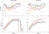 |
Fig. 19. Stellar velocity curves of the LMC evolutionary phases. Top and bottom panels show the radial motions and rotation curves, respectively, for both NN complete (left) and NN optimal samples (right). Coloured lines are for the eight evolutionary phases. Only bins with more than 500 sources are plotted. |
6. Conclusions
In this work, we analyse the velocity maps of four LMC samples, defined using different selection strategies, namely, the proper motion selection, as in MC21, and three samples based on a neural network classification, trained using a MW+LMC simulation created by GOG. Using different probability cuts, Pcut, we defined two LMC samples: NN complete, with Pcut = 0.01, and NN optimal, with Pcut = 0.52, corresponding to the optimal value based on the receiver operating characteristics (ROC) curve. We applied to this last sample an extra cut on the apparent G magnitude of G < 19.5 mag, in order to remove further contamination of misclassified faint stars. Taking advantage of the recently released spectroscopic line-of-sight velocities published in Gaia DR3, we generated sub-samples that include both proper motions and line-of-sight velocities. We also adopt a new formalism in order to transform from the observable space (α, δ, μα*, μδ, Vlos) to the LMC frame (x′,y′,z′,vx′, vy′, vz′). The advantage of this formalism based on that of van der Marel & Cioni (2001) and van der Marel et al. (2002) is the possibility to include the Vlos component when deriving internal LMC velocities.
We analysed the velocity profile and maps in the LMC coordinate system for the full samples and the Vlos sub-samples. The velocity maps corresponding to the radial and tangential component of the velocity for the PM sample are analogous to those presented in the MC21 paper, while in Sect. 4.3, we analysed the differences between the samples based on a NN classification. As shown, differences are of second order and mainly located in the outer disc, where differences in density also arise. As a novelty, we also include the Vlos sub-samples with line-of-sight velocities from Gaia DR3 (Katz et al. 2022), which allows for the analysis of the vertical velocity component.
The main conclusions of this work are as follow:
-
In all samples and sub-samples, the dynamics in the inner disc are mainly dominated by the bar, and this is a confirmation of what was first found in MC21. An asymmetry along the bar-major axis is emphasised, especially when mapping the kinematics with the Vlos sub-samples.
-
The kinematics on the spiral arm overdensity seem to be dominated by an inward (VR < 0) motion and a rotation faster than that of the disc (
 ) in the part of the arm attached to the bar, although Vlos sub-samples are not conclusive in this region.
 -
The dynamics seems to change in the part of the arm with lower density or even detached from the main arm after the density break, in the sense that the radial velocity and residual tangential velocity can reverse signs.
-
The contamination of MW stars seems to dominate the outer parts of the disc, mainly affecting older and later evolutionary phases (e.g.,, RRL or AGB stars).
-
Uncertainties in the LMC systemic motion largely affect the vertical component of the velocity, even causing a change in sign. Uncertainties in the morphological parameters of the LMC (inclination and position angle) can modify the radial and vertical velocity maps, apart from inducing a stretch or rotation of them.
-
The lack of a Vlos value for all stars does not substantially impact the kinematic profiles or maps. The approximation used to derive the internal kinematics is accurate.
The available Gaia DR3 dataset and the new strategy to select LMC clean samples have proven to be suitable to performing kinematic studies and allowing for a deep analysis of the nature of the LMC morphology. Comparisons with realistic LMC mock catalogues are crucial and this will be the focus of further work.
Movies
Animation 1 (01.i_maps) Access Supplementary Material
Animation 2 (02.theta_maps) Access Supplementary Material
Animation 3 (03.i_profiles) Access Supplementary Material
Animation 4 (04.theta_profiles) Access Supplementary Material
Animation 5 (05.mux0_maps_profiles) Access Supplementary Material
Animation 6 (06.muy0_maps_profiles) Access Supplementary Material
Animation 7 (07.muz0_maps_profiles) Access Supplementary Material
Note that the difference in the number of sources with the ones in MC21 comes from the different cut in radius, now being of 15° instead of 20°.
Readers interested in using the Neural Network developed in the paper can contact the corresponding author.
Animations of the variation of the morphological parameters and systemic motion in the velocity profile and maps are made available https://www.aanda.org/10.1051/0004-6361/202244601/olm.
Acknowledgments
This work has made use of data from the European Space Agency (ESA) mission Gaia (https://www.cosmos.esa.int/gaia), processed by the Gaia Data Processing and Analysis Consortium (DPAC, https://www.cosmos.esa.int/web/gaia/dpac/consortium). Funding for the DPAC has been provided by national institutions, in particular the institutions participating in the Gaia Multilateral Agreement. OJA acknowledges funding by l’Agència de Gestió d’Ajuts Universitaris i de Recerca (AGAUR) official doctoral program for the development of a R+D+i project under the FI-SDUR grant (2020 FISDU 00011). O.J.A., M.R.G., X.L., T.A. and E.M. acknowledge funding by the Spanish MICIN/AEI/10.13039/501100011033 and by “ERDF A way of making Europe” by the “European Union” through Grant RTI2018-095076-B-C21, and the Institute of Cosmos Sciences University of Barcelona (ICCUB, Unidad de Excelencia ‘María de Maeztu’) through Grant CEX2019-000918-M. TA also acknowledges the Grant RYC2018-025968-I funded by MCIN/AEI/10.13039/501100011033 and by “ESF Investing in your future”. PM acknowledges support from project Grants from the Swedish Research Council (Vetenskaprådet, Reg: 2017- 03721; 2021-04153). L.C. acknowledges financial support from the Chilean Agencia Nacional de Investigación y Desarrollo (ANID) through Fondo Nacional de Desarrollo Científico y Tecnológico (FONDECYT) Regular Project 1210992. SRF acknowledges financial support from the Spanish Ministry of Economy and Competitiveness (MINECO) under Grant number AYA2016-75808-R, RTI2018-096188-B-I00, from the CAM-UCM under Grant number PR65/19-22462 and the Spanish postdoctoral fellowship (2017-T2/TIC-5592).
References
- Anders, F., Khalatyan, A., Queiroz, A. B. A., et al. 2022, A&A, 658, A91 [NASA ADS] [CrossRef] [EDP Sciences] [Google Scholar]
- Athanassoula, E. 1980, A&A, 88, 184 [NASA ADS] [Google Scholar]
- Choi, Y., Nidever, D. L., Olsen, K., et al. 2018, ApJ, 866, 90 [Google Scholar]
- Choi, Y., Olsen, K. A. G., Besla, G., et al. 2022, ApJ, 927, 153 [NASA ADS] [CrossRef] [Google Scholar]
- Cioni, M. R. L., Clementini, G., Girardi, L., et al. 2011, A&A, 527, A116 [CrossRef] [EDP Sciences] [Google Scholar]
- Cullinane, L. R., Mackey, A. D., Da Costa, G. S., et al. 2022a, MNRAS, 510, 445 [Google Scholar]
- Cullinane, L. R., Mackey, A. D., Da Costa, G. S., et al. 2022b, MNRAS, 512, 4798 [NASA ADS] [CrossRef] [Google Scholar]
- Cusano, F., Moretti, M. I., Clementini, G., et al. 2021, MNRAS, 504, 1 [NASA ADS] [CrossRef] [Google Scholar]
- Elmegreen, D. M., & Elmegreen, B. G. 1980, AJ, 85, 1325 [NASA ADS] [CrossRef] [Google Scholar]
- Gaia Collaboration (Helmi, A., et al.) 2018, A&A, 616, A12 [NASA ADS] [CrossRef] [EDP Sciences] [Google Scholar]
- Gaia Collaboration (Luri, X., et al.) 2021a, A&A, 649, A7 [EDP Sciences] [Google Scholar]
- Gaia Collaboration (Brown, A. G. A., et al.) 2021b, A&A, 649, A1 [NASA ADS] [CrossRef] [EDP Sciences] [Google Scholar]
- Gallagher, J. S. I., & Hunter, D. A. 1984, ARA&A, 22, 37 [NASA ADS] [CrossRef] [Google Scholar]
- Garma-Oehmichen, L., Martinez-Medina, L., Hernández-Toledo, H., & Puerari, I. 2021, MNRAS, 502, 4708 [NASA ADS] [CrossRef] [Google Scholar]
- Goldreich, P., & Lynden-Bell, D. 1965, MNRAS, 130, 125 [Google Scholar]
- Haschke, R., Grebel, E. K., & Duffau, S. 2012, AJ, 144, 106 [NASA ADS] [CrossRef] [Google Scholar]
- Julian, W. H., & Toomre, A. 1966, ApJ, 146, 810 [NASA ADS] [CrossRef] [Google Scholar]
- Kallivayalil, N., van der Marel, R. P., Besla, G., Anderson, J., & Alcock, C. 2013, ApJ, 764, 161 [Google Scholar]
- Katz, D., Sartoretti, P., Guerrier, A., et al. 2022, A&A, submited, ArXiv e-prints [arXiv:2206.05902] [Google Scholar]
- Lin, C. C., & Shu, F. H. 1964, ApJ, 140, 646 [Google Scholar]
- Lindblad, P. O. 1960, Stockholms Observatoriums Annaler, 4, 4 [NASA ADS] [Google Scholar]
- Lindegren, L., Bastian, U., Biermann, M., et al. 2021a, A&A, 649, A4 [EDP Sciences] [Google Scholar]
- Lindegren, L., Klioner, S. A., Hernández, J., et al. 2021b, A&A, 649, A2 [EDP Sciences] [Google Scholar]
- Luri, X., Palmer, M., Arenou, F., et al. 2014, A&A, 566, A119 [NASA ADS] [CrossRef] [EDP Sciences] [Google Scholar]
- Nidever, D. L., Olsen, K., Walker, A. R., et al. 2017, AJ, 154, 199 [Google Scholar]
- Niederhofer, F., Cioni, M.-R. L., Schmidt, T., et al. 2022, MNRAS, 512, 5423 [NASA ADS] [CrossRef] [Google Scholar]
- Olsen, K. A. G., & Salyk, C. 2002, AJ, 124, 2045 [NASA ADS] [CrossRef] [Google Scholar]
- Pedregosa, F., Varoquaux, G., Gramfort, A., et al. 2011, J. Mach. Learn. Res., 12, 2825 [Google Scholar]
- Pietrzyński, G., Graczyk, D., Gallenne, A., et al. 2019, Nature, 567, 200 [Google Scholar]
- Ripepi, V., Chemin, L., Molinaro, R., et al. 2022, MNRAS, 512, 563 [NASA ADS] [CrossRef] [Google Scholar]
- Roca-Fàbrega, S., Valenzuela, O., Figueras, F., et al. 2013, MNRAS, 432, 2878 [Google Scholar]
- Roca-Fàbrega, S., Antoja, T., Figueras, F., et al. 2014, MNRAS, 440, 1950 [CrossRef] [Google Scholar]
- Romero-Gómez, M., Athanassoula, E., Masdemont, J. J., & García-Gómez, C. 2007, A&A, 472, 63 [NASA ADS] [CrossRef] [EDP Sciences] [Google Scholar]
- Salo, H., Laurikainen, E., Buta, R., & Knapen, J. H. 2010, ApJ, 715, L56 [NASA ADS] [CrossRef] [Google Scholar]
- Schmidt, T., Cioni, M.-R. L., Niederhofer, F., et al. 2020, A&A, 641, A134 [NASA ADS] [CrossRef] [EDP Sciences] [Google Scholar]
- Schmidt, T., Cioni, M.-R. L., Niederhofer, F., et al. 2022, A&A, 663, A107 [NASA ADS] [CrossRef] [EDP Sciences] [Google Scholar]
- Toomre, A. 1981, in Structure and Evolution of Normal Galaxies, eds. S. M. Fall, & D. Lynden-Bell, 111 [Google Scholar]
- Toomre, A., & Toomre, J. 1972, ApJ, 178, 623 [Google Scholar]
- van der Marel, R. P. 2001, AJ, 122, 1827 [Google Scholar]
- van der Marel, R. P., & Cioni, M.-R. L. 2001, AJ, 122, 1807 [Google Scholar]
- van der Marel, R. P., & Kallivayalil, N. 2014, ApJ, 781, 121 [Google Scholar]
- van der Marel, R. P., Alves, D. R., Hardy, E., & Suntzeff, N. B. 2002, AJ, 124, 2639 [NASA ADS] [CrossRef] [Google Scholar]
- Vasiliev, E. 2018, MNRAS, 481, L100 [Google Scholar]
- Wan, Z., Guglielmo, M., Lewis, G. F., Mackey, D., & Ibata, R. A. 2020, MNRAS, 492, 782 [Google Scholar]
- Yozin, C., & Bekki, K. 2014, MNRAS, 439, 1948 [Google Scholar]
- Zaritsky, D. 2004, ApJ, 614, L37 [NASA ADS] [CrossRef] [Google Scholar]
- Zivick, P., Kallivayalil, N., Besla, G., et al. 2019, ApJ, 874, 78 [Google Scholar]
Appendix A: Coordinate changes
In this appendix, we detail the steps performed to transform from heliocentric equatorial coordinates to LMC internal coordinates. This formalism is based on van der Marel & Cioni (2001) and van der Marel et al. (2002).
A.1. Positions
The position of any point in space is uniquely determined by its right ascension and declination on the sky, (α, δ), and its distance, D, which can be referenced to a particular point, O, with coordinates (α0, δ0, D0). We chose the LMC centre to be the reference centre.
We introduce the angular coordinates (ϕ, ρ) (Figure 10) which are defined in the celestial sphere:
-
is the angular distance between the points (α, δ) and (α0, δ0).
-
is the position angle of the point (α, δ) with respect to (α0, δ0). In particular, ϕ is the angle at (α0, δ0) between the tangent to the great circle on the celestial sphere through (α, δ) and (α0, δ0), and the circle of constant declination δ0. By convention, ϕ is measured counterclockwise starting from the axis that runs in the direction of decreasing right ascension at constant declination δ0.
We can uniquely define (ρ, ϕ) as function of (α, δ), for a choice of the origin O, by using:
![Mathematical equation: $$ \begin{aligned} \begin{aligned} \rho =&\arccos \left[ \cos \delta \cos \delta _0 \cos (\alpha -\alpha _0) + \sin \delta \sin \delta _0 \right], \\ \phi =&\arctan \left[ \frac{\sin \delta \cos \delta _0 - \cos \delta \sin \delta _0 \cos (\alpha -\alpha _0)}{-\cos \delta \sin (\alpha - \alpha _0)} \right] \end{aligned} .\end{aligned} $$](/articles/aa/full_html/2023/01/aa44601-22/aa44601-22-eq14.gif) (A.1)
(A.1)
These previous equations have been obtained by using the cosine, sine rule of spherical trigonometry and the so-called analogue formula:
 (A.2)
(A.2)
Then, we can introduce a Cartesian coordinate system (x, y, z) that has its origin at O, with the x-axis anti-parallel to the right ascension axis, the y-axis parallel to the declination axis, and the z-axis towards the observer. This is somehow similar to considering the orthographic projection -a method of representing 3D objects where the object is viewed along parallel lines that are perpendicular to the plane of the drawing of the usual celestial coordinates and proper motions. This yields the following transformations:
 (A.3)
(A.3)
A second Cartesian coordinate system (x′,y′,z′) is then introduced. It is obtained from the system (x, y, z) by counterclockwise rotation around the z-axis by an angle θ, followed by a clockwise rotation around the new x′-axis by an angle i. With this definition, the (x′,y′) plane is inclined with respect to the sky by an angle, i, (with face-on viewing corresponding to i = 0°). The angle, θ, is the position angle of the line-of-nodes - the intersection of the (x′,y′)-plane, and the (x, y)-plane of the sky, measured counterclockwise from the x-axis. In practice, i and θ ought to be chosen such that the (x′,y′)-plane coincides with the plane of the LMC disk. The transformations between the (x′,y′,z′) and the (x, y, z) coordinates are represented by:
 (A.4)
(A.4)
The distance, D, of points in the (x′,y′) plane is of interest here, as a function of the position (ρ, ϕ) on the sky. The points in this plane fulfil z′ = 0, which yields:
 (A.5)
(A.5)
A.2. Velocities
At any given position (D, ρ, ϕ) a velocity vector can be decomposed into a sum of three orthogonal components:
 (A.6)
(A.6)
Here, v1 is the line-of-sight velocity and v2 and v3 are the velocity components in the plane of the sky. Computing the time derivative of Eq. (A.3) yields:
 (A.7)
(A.7)
where (vx, vy, vz) is the three-dimensional velocity in the (x, y, z) coordinate system. Again, to describe the internal kinematic of the galaxy it is useful to adopt the second Cartesian coordinate system (x′,y′,z′). We recall that the (x′,y′)-plane coincides with the plane of the LMC disk. Upon taking the time derivative on both sides on Eq. (A.4) yields the transformation equations from (vx, vy, vz) to  . This result can be used with Eq. (A.7) to obtain:
 (A.8)
(A.8)
We know that v1 is the line-of-sight velocity. Now, we need to relate the velocities v2 and v3 with the proper motions μα* and μδ. In these directions, the proper motions are defined as:
 (A.9)
(A.9)
Upon taking time derivative of Eq. (A.2) we obtain relations between dρ/dt and dϕ/dt on the one hand, and dα/dt and dδ/dt on the other. This system can be solved to obtain:
 (A.10)
where the angle Γ determines the rotation angle of the (v2, v3) frame on the sky. It is given by:
![Mathematical equation: $$ \begin{aligned} \begin{aligned} \cos \Gamma&= [\sin \delta \cos \delta _0 \cos (\alpha -\alpha _0) - \cos \delta \sin \delta _0] / \sin \rho , \\ \sin \Gamma&= [\cos \delta _0 \sin (\alpha -\alpha _0)] / \sin \rho . \end{aligned} \end{aligned} $$](/articles/aa/full_html/2023/01/aa44601-22/aa44601-22-eq25.gif) (A.11)
(A.11)
A.2.1. Correcting from the systemic motion
For a planar system, the velocity of a tracer can be written as a sum of three components: the velocity corresponding to the systemic motion, the velocity corresponding to precession and nutation of the disk plane, and the velocity corresponding to the internal motion of the tracer:
 (A.12)
Then, if we neglect the effect of precession and nutation, we can determine the internal motion by using:
 (A.13)
where we explain how to compute the first term in Section A.2. On the other hand, we can determine the systemic motion using the inverse relation of Eq. (A.7):
 (A.14)
where μx, 0 and μy, 0 are the associated proper motions in the x and y directions at the centre of the disc, and μz, 0 = vz, 0/D0, the associated line-of-sight velocity, expressed on the same scale as the proper motions by dividing by D0.
A.3. Estimating the observational line-of-sight velocity
In a case where we do not have observational information on the line-of-sight velocity, we can estimate v1, int by computing the derivative of the distance as function of time:
![Mathematical equation: $$ \begin{aligned} \begin{aligned} v_{1,int} \equiv&\frac{dD}{dt} = \frac{d}{dt} \left[ \frac{D_0 \cos i}{\cos i \cos \rho - \sin i \sin \rho \sin (\phi -\theta )} \right] \\ =&\frac{v_{2,int} [\cos i \sin \rho + \sin i \cos \rho \sin (\phi - \theta )] + v_{3,int} \sin i \cos (\phi - \theta )}{\cos i \cos \rho - \sin i \sin \rho \sin (\phi - \theta )} \end{aligned} .\end{aligned} $$](/articles/aa/full_html/2023/01/aa44601-22/aa44601-22-eq29.gif) (A.15)
(A.15)
To compute v2, int and v3, int when observational information on the line-of-sight velocity is lacking, we proceed the way that is described in Section A.2, since v2, int and v3, int only depend on the proper motions.
All Tables
Comparison of the LMC samples number of sources and mean astrometry between the proper motion selection (MC21) and the neural networks.
Matches of the classified LMC members in our four considered samples against the validation samples.
All Figures
|
Fig. 1. Characteristics of the GOG simulated samples. Top left and middle: distribution of proper motions in right ascension and declination, respectively. In orange and blue: LMC and the MW training samples. Top right: parallax distribution. Bottom left: magnitude G distribution of the simulated samples. Bottom middle and right: colour-magnitude diagram of the LMC and MW, respectively. Colors represent relative stellar density, with darker colors meaning higher densities. |
| In the text | |
|
Fig. 2. Comparison between the Gaia base and training samples. Top from left to right: density distribution in equatorial coordinates of the Gaia base and Gaia training samples in logarithmic scale, parallax, and G magnitude distributions. Bottom from left to right: proper motion distributions in right ascension and declination and colour-magnitude diagrams for the Gaia base and training samples. In the histograms, in gray we show the Gaia base sample, while in dotted purple we show the Gaia training sample. In the color-magnitude diagrams, colors represent relative stellar density with darker colors meaning higher densities. |
| In the text | |
|
Fig. 3. Evaluation metrics for the Neural Network classifier performance. Left: ROC curve. Black dot is in the “elbow” of the ROC curve and it shows the best balance between completeness and purity. The purple star shows the completeness threshold. Right: precision-recall curve. In both cases, we compare our model (orange solid curve) with a classifier that has no class separation capacity (blue dashed curve). |
| In the text | |
|
Fig. 4. Probability distribution of the Gaia base sample for the NN classifier. A probability value close to 1 (0) means a high probability of being a LMC (MW) star. |
| In the text | |
|
Fig. 5. Sky density distribution in equatorial coordinates of both the LMC (left) and MW (right) sample obtained from the different classifiers. First row: proper motion selection classification. Second row: Complete NN classification. Third row: optimal NN classification. Fourth row: truncated-optimal NN classification. Note: in the fourth row, we display a cut in magnitude G > 19.5 for both the LMC and MW samples and, therefore, the total number of stars is reduced. |
| In the text | |
|
Fig. 6. Astrometric and photometric characteristics of the LMC and MW samples. From left to right: PM sample, NN complete, NN optimal and NN truncated-optimal samples. In the first four rows, we show distributions of proper motion in right ascension and declination, parallax, and G magnitude, respectively, of the LMC (orange) and MW (blue) samples. In the last two rows, we show the colour-magnitude diagram of the samples classified as LMC and MW, respectively. Color represents the relative stellar density, with darker colors meaning higher densities. |
| In the text | |
|
Fig. 7. Distance distribution of the StarHorse validation sample. In blue (orange), the StarHorse stars classified as MW (LMC) according to the d = 40 kpc criteria. |
| In the text | |
|
Fig. 8. Evaluation metrics for the Neural Network classifier performance using the StarHorse sample. Left: ROC curve. Black dot is in the “elbow” of the ROC curve and it shows the best balance between completeness and purity. Right: precision-recall curve. In both cases, we compare our model (orange solid curve) with a classifier that has no class separation capacity (blue dashed curve). |
| In the text | |
|
Fig. 9. Line-of-sight velocity distribution for the stars classified as LMC (top) and MW (bottom). We show the three Vlos sub-samples of the PM selection (left), NN complete (middle) and NN optimal (right) samples. |
| In the text | |
|
Fig. 10. Schematic view of the observer-galaxy system. The LMC center O(α0, δ0, D0) is chosen to be the origin O of the (x, y, z) coordinate system. Top: projected view of the sky. All vectors and angles lie in the plane of the paper. The angles ρ and ϕ define the projected position on the sky of a given point with coordinates (α, δ). Bottom: side view of the observer-galaxy system. The distance from the observer to the LMC center is D0 and the distance from the observer to an object is D. The component v1 lies along the line-of-sight and points away from the observer. |
| In the text | |
|
Fig. 11. Schematic representation of the reference frames used, all of them centred on the LMC centre (α0, δ0). In blue, we show the orthographic reference frame, (x, y, z), whereas in red, we show the Cartesian LMC frame, (x′,y′,z′). We also show the position of a real star (solid dark gray), its projection in the LMC cartesian frame under the imposition of z′ = 0 (red frame). |
| In the text | |
|
Fig. 12. Comparison between density and overdensity maps. Top: LMC density map for the NN complete sample. Bottom: LMC overdensity map for a 0.4 kpc-bandwidth KDE. A black line splitting the overdensities from the underdensities is plotted. Both maps are shown in the (x′,y′) Cartesian coordinate system. |
| In the text | |
|
Fig. 13. Simulation B5. First row left panel: density distribution in logarithmic scale. First row, right panel: velocity profiles of the B5 simulation. In blue, orange and green, for the radial, tangential, and vertical components, respectively, when taking into account the full velocity information (dashed lines), or when Vlos is not available (solid lines). Differences are negligible and both curves overlap. Scatter points show the real velocity profiles. Second row: N-body simulation maps (left, radial; middle, residual tangential; right, vertical), without applying any coordinate transformation. Third row: same as above computed applying the (Sect. 3) coordinate transformations without line-of-sight information. Fourth row: same as above computed applying the (Sect. 3) coordinate transformations with line-of-sight information. The black line shows the contour corresponding to overdensity equal to zero for a 0.4 kpc-bandwidth KDE (see details in Sect. 4.2). |
| In the text | |
|
Fig. 14. Velocity profiles for the four LMC samples in the case Vlos is not available (left) and when it is available (right). From top to bottom: radial, tangential, and vertical velocity profiles. Each curve corresponds to one LMC sample: PM selection (blue), NN complete (orange), NN optimal (green) and NN truncated-optimal (red). In black, the radial and rotation curve published in MC21 (their Fig. 14) is shown. For most of the bins, the error bar is small and cannot be seen. Only bins with more than 300 sources are plotted. |
| In the text | |
|
Fig. 15. LMC median radial velocity maps. All maps are shown in the (x′,y′) Cartesian coordinate system. From top to bottom: PM sample, NN complete, NN optimal, and NN truncated-optimal sample. Left: line-of-sight velocity not included. Right: line of sight velocity included. NN truncated-optimal Vlos sub-sample map is not shown because it is the same as the NN optimal Vlos sub-sample (see text for details). For each colormap, a black line splitting the overdensities from the underdensities for a 0.4 kpc-bandwidth KDE is plotted and a minimum number of 3 (20) stars per bin is imposed when the line-of-sight is (not) considered. |
| In the text | |
|
Fig. 16. LMC median residual tangential velocity maps. All maps are shown in the (x′,y′) Cartesian coordinate system. From top to bottom: PM sample, NN complete, NN optimal, and NN truncated-optimal sample. Left: line-of-sight velocity not included. Right: line-of-sight velocity included. NN truncated-optimal Vlos sub-sample map is not shown because it is the same as the NN optimal Vlos sub-sample (see text for details). For each colormap, a black line splitting the overdensities from the underdensities for a 0.4kpc-bandwidth KDE is plotted and a minimum number of 3 (20) stars per bin is imposed when the line-of-sight is (not) considered. |
| In the text | |
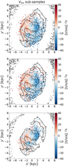 |
Fig. 17. Same as Fig. 15 for the median vertical velocity of the Vlos sub-samples. |
| In the text | |
|
Fig. 18. Stellar vertical velocity profiles of the LMC Vlos sub-samples (blue, orange and green for the PM, NN complete, and NN optimal samples, respectively) for different input values of μz, 0: the Gaia DR3 derived in solid lines and the MC21 adopted value in dashed lines (values given in the legend). |
| In the text | |
|
Fig. 19. Stellar velocity curves of the LMC evolutionary phases. Top and bottom panels show the radial motions and rotation curves, respectively, for both NN complete (left) and NN optimal samples (right). Coloured lines are for the eight evolutionary phases. Only bins with more than 500 sources are plotted. |
| In the text | |
Current usage metrics show cumulative count of Article Views (full-text article views including HTML views, PDF and ePub downloads, according to the available data) and Abstracts Views on Vision4Press platform.
Data correspond to usage on the plateform after 2015. The current usage metrics is available 48-96 hours after online publication and is updated daily on week days.
Initial download of the metrics may take a while.