| Issue |
A&A
Volume 688, August 2024
|
|
|---|---|---|
| Article Number | A51 | |
| Number of page(s) | 20 | |
| Section | Galactic structure, stellar clusters and populations | |
| DOI | https://doi.org/10.1051/0004-6361/202349058 | |
| Published online | 30 July 2024 | |
KRATOS: A large suite of N-body simulations to interpret the stellar kinematics of LMC-like discs⋆
1
Departament de Física Quàntica i Astrofísica (FQA), Universitat de Barcelona (UB), C Martí i Franquès, 1, 08028 Barcelona, Spain
e-mail: This email address is being protected from spambots. You need JavaScript enabled to view it.
2
Institut de Ciències del Cosmos (ICCUB), Universitat de Barcelona, Martí i Franquès 1, 08028 Barcelona, Spain
3
Institut d’Estudis Espacials de Catalunya (IEEC), c. Esteve Terradas 1, 08860 Castelldefels (Barcelona), Spain
4
Lund Observatory, Division of Astrophysics, Lund University, Box 43 221 00 Lund, Sweden
5
Departamento de Física de la Tierra y Astrofísica, UCM, and IPARCOS, Facultad de Ciencias Físicas, Plaza Ciencias, 1, Madrid 28040, Spain
6
School of Physics & Astronomy, University of Leicester, University Road, Leicester LE1 7RH, UK
7
Instituto de Astrofísica, Universidad Andres Bello, Fernandez Concha 700, Las Condes, Santiago RM, Chile
Received:
21
December
2023
Accepted:
22
March
2024
Abstract
Context. The Large and Small Magellanic Clouds (LMC and SMC, respectively) are the brightest satellites of the Milky Way (MW), and for the last thousand million years they have been interacting with one another. As observations only provide a static picture of the entire process, numerical simulations are used to interpret the present-day observational properties of these kinds of systems, and most of them have been focused on attempting to recreate the neutral gas distribution and characteristics through hydrodynamical simulations.
Aims. We present KRATOS, a comprehensive suite of 28 open-access pure N-body simulations of isolated and interacting LMC-like galaxies designed for studying the formation of substructures in their discs after interaction with an SMC-mass galaxy. The primary objective of this paper is to provide theoretical models that help us to interpret the formation of general structures in an LMC-like galaxy under various tidal interaction scenarios. This is the first paper of a series dedicated to the analysis of this complex interaction.
Methods. Simulations are grouped into 11 sets of up to three configurations, with each set containing (1) a control model of an isolated LMC-like galaxy; (2) a model that contains the interaction with an SMC-mass galaxy, and (3) a model where both an SMC-mass and a MW-mass galaxy may interact with the LMC-like galaxy (the most realistic model). In each simulation, we analysed the orbital history between the three galaxies and examined the morphological and kinematic features of the LMC-like disc galaxy throughout the interaction. This includes investigating the disc scale height and velocity maps. When a bar was found to develop, we characterised its strength, length, off-centredness, and pattern speed.
Results. The diverse outcomes found in the KRATOS simulations, including the presence of bars, warped discs, and various spiral arm shapes, demonstrate the opportunities they offer to explore a range of LMC-like galaxy morphologies. These morphologies directly correspond to distinct disc kinematic maps, making them well-suited for a first-order interpretation of the LMC’s kinematic maps. From the simulations, we note that tidal interactions can: boost the disc scale height; both destroy and create bars; and naturally explain the off-centre stellar bars. The bar length and pattern speed of long-lived bars are not appreciably altered by the interaction.
Conclusions. The high spatial, temporal, and mass resolution used in the KRATOS simulations has been shown to be appropriate for the purpose of interpreting the internal kinematics of LMC-like discs, as evidenced by the first scientific results presented in this work.
Key words: galaxies: interactions / galaxies: kinematics and dynamics / Magellanic Clouds / galaxies: structure
Movies are available at https://www.aanda.org.
© The Authors 2024
 Open Access article, published by EDP Sciences, under the terms of the Creative Commons Attribution License (https://creativecommons.org/licenses/by/4.0), which permits unrestricted use, distribution, and reproduction in any medium, provided the original work is properly cited.
This article is published in open access under the Subscribe to Open model. This email address is being protected from spambots. You need JavaScript enabled to view it. to support open access publication.
1. Introduction
Only a few extragalactic stellar structures are visible to the naked eye from Earth. The brightest of those are the Magellanic Clouds (MCs), which are the most massive of the Milky Way (MW) satellite galaxies. Because they are so close, the Large and Small Magellanic Clouds (LMC and SMC, respectively) provide astronomers with a unique window onto the complexities of extragalactic systems. Furthermore, the evident large-scale structures they contain, in particular the disc-like structure, the spiral arm, and the bar in the LMC (e.g. Elmegreen & Elmegreen 1980; Gallagher & Hunter 1984; Yozin & Bekki 2014), and the stellar bridge that connects both galaxies (e.g. Harris 2007; Kallivayalil et al. 2013; Zivick et al. 2019; Gaia Collaboration 2021b), make the LMC–SMC system an ideal laboratory for studying the effects of galactic interactions on the evolution of dwarf galaxies and their structures with the data provided at present by the Gaia mission (Gaia Collaboration 2016, 2021a), the VISTA survey of the Magellanic Clouds system (VMC, Cioni et al. 2011), and the Survey of the Magellanic Stellar History (SMASH, Nidever et al. 2017), to name a few. Additionally, more data are anticipated in the future thanks to projects like Euclid (Amiaux et al. 2012; Euclid Collaboration 2022), the Vera C. Rubin Observatory (previously referred to as Large Synoptic Survey Telescope or LSST, Ivezić et al. 2019), the Sloan Digital Sky Survey-V (SDSS-V, Kollmeier et al. 2019; Almeida et al. 2023), and the 4-m Multi-Object Spectrograph Telescope (4MOST, de Jong et al. 2019).
The LMC is so peculiar that it gives its name to a type of galaxy, the barred Magellanic spirals (BMSs; de Vaucouleurs & Freeman 1972). The LMC itself is a dwarf bulgeless spiral galaxy with a single spiral arm, an off-centred and asymmetric stellar bar, and many star-forming regions (e.g. Elmegreen & Elmegreen 1980; Gallagher & Hunter 1984; Zaritsky 2004; Yozin & Bekki 2014; Gaia Collaboration 2021b). It is also a gas-rich galaxy (e.g. Luks & Rohlfs 1992; Kim et al. 1998) characterised by an inclined disc (e.g. van der Marel & Cioni 2001; van der Marel 2001), with multiple warps reported (e.g. Olsen & Salyk 2002; Nikolaev et al. 2004; Choi et al. 2018b; Saroon & Subramanian 2022; Ripepi et al. 2022). The LMC lies at a distance of around 50 kpc (Pietrzyński et al. 2019). The SMC has long been thought to be a satellite of the LMC due to its proximity. It is at around 62 kpc from the MW (e.g. Cioni et al. 2000; Hilditch et al. 2005; Graczyk et al. 2014) and 20–25 kpc away from the LMC. The SMC is a gas-rich irregular dwarf galaxy (e.g. Rubio et al. 1993; Staveley-Smith et al. 1998), and features a low-metallicity environment (e.g. Choudhury et al. 2018; Grady et al. 2021). An attempt to reconstruct its 3D shape was made using red-clump stars and other standard candles, revealing that it is elongated and stretches over about approximately 15–30 kpc in the east-northeast–southwest direction (e.g. Subramanian & Subramaniam 2012; Ripepi et al. 2017).
Because of a lack of high-precision astrometric data, it has been difficult to study the complex interaction between these two satellite galaxies and the MW. With the available data at the time, and using theoretical models, many authors suggested that the MCs were indeed orbiting the MW, and that they had experienced multiple pericentric passages (e.g. Tremaine 1976; Murai & Fujimoto 1980; Lin & Lynden-Bell 1982; Gardiner et al. 1994). This conclusion was accepted for many years, until new data revealed a different history. The scenario that is presently accepted was proposed by Besla et al. (2007) based on data from the Hubble Space Telescope (Kallivayalil et al. 2006b,a) and theoretical models that showed that the MCs are most probably in the aftermath of their first approach to the MW, with no prior pericentre passages within the last 10 Gyr. Moreover, the authors showed that the orbits of these two galactic systems around the MW are highly eccentric, with apocentres well beyond 200 kpc, and with orbital periods exceeding 5 Gyr. The date of the first pericentre is still a matter of debate; for instance, Vasiliev (2024) claims that a scenario in which the LMC is on its second passage around the MW (that would have occurred 5–10 Gyr ago at a distance of ≳100 kpc) is consistent with current observational constraints on the mass distribution and relative velocity of both galaxies (see also Patel et al. 2017, 2020).
Focusing now on the LMC–SMC system, there is also controversy as to when the most recent interaction between the two satellites began. Gardiner & Noguchi (1996) stated that the most recent near encounter between the two MCs took place somewhere in between 150 and 200 Myr ago and that there were less than 10 kpc between them at their closest point of encounter. These authors also showed that this interaction would have led to the formation of the tidal structure known as the Magellanic bridge, which is a structure found in the region between the two galaxies (e.g. Kerr et al. 1954; Misawa et al. 2009). First, Hindman et al. (1963) found that this tidal structure contains neutral hydrogen, suggesting that it formed recently and could host active star formation. Decades later, a stellar population of blue main sequence stars in the bridge was discovered by Irwin et al. (1985), confirming that star formation is ongoing within this structure. In recent years, the Magellanic Bridge has been studied using both simulations (e.g. Besla et al. 2012; Diaz & Bekki 2012) and observations (e.g. Harris 2007; Kallivayalil et al. 2013; Bagheri et al. 2013; Noël et al. 2013; Skowron et al. 2014; Carrera et al. 2017; Zivick et al. 2019; Schmidt et al. 2020; Gaia Collaboration 2021b) in an attempt to learn about its formation mechanism and to use it to better understand the complex interaction between the two satellite galaxies.
The presently available observational data are insufficient to study the formation and evolution of the LMC–SMC system. Observations give us only a static picture of the whole process, and that is why most researchers studying these kinds of systems use numerical simulations. These studies have naturally been focused on trying to recreate the distribution of neutral gas and the position and properties of the streams using N-body simulations that include hydrodynamics, with the goal being to reproduce the whole past interaction process.
For instance, Pardy et al. (2018) presented hydrodynamic simulations designed to reproduce the observations of Hammer et al. (2015) that showed that the Magellanic Stream is made up of two filaments (e.g. Putman et al. 2003; Nidever et al. 2008). Pardy et al. (2018) suggested that, to reproduce the observations, the MCs must have been more gas-rich in the past, and that the gas stripping efficiency of the LMC must have been much higher. Later, Wang et al. (2019) showed, for the first time, that a physical model is capable of explaining and reproducing the enormous quantities of gas stripped from the MCs, namely more than 50 per cent of their initial content. More recently, Tepper-García et al. (2019) included, for the first time, a weakly magnetised and spinning Magellanic Corona, a halo of warm gas surrounding the LMC and SMC, in their simulations to reproduce the location and the extension of the Magellanic Stream on the sky. Lucchini et al. (2020) also included a Magellanic Corona to show that its presence can explain the ionised gas component of the Magellanic Stream. Finally, Lucchini et al. (2021) present new simulations of the formation of the Magellanic Stream with a new first-passage interaction history of the MCs, where the orientation of the orbit of the SMC around the LMC is qualitatively different and leads to a different 3D spatial positioning of the Stream compared to previous models. Their simulated Stream is only ∼20 kpc away from the Sun at its closest point, whereas previous first-infall models predicted a distance of 100–200 kpc.
Similarly, the study of the interaction between the MCs and the MW cannot only rely on observations, but again requires the use of numerical simulations. As mentioned, several N-body simulations have been run and used to analyse the effect of the MCs (or more specifically the LMC) on the MW (e.g. Garavito-Camargo et al. 2019; Petersen & Peñarrubia 2021) and to determine the past orbits of the MCs (e.g. Vasiliev 2023, 2024). However, studies of the effect of these interactions on the internal structures of the LMC-like disc, the bar, and the spiral arm have only been carried out by a few authors. In particular, only the work by Besla et al. (2012) extensively explored these features in simulations. Understanding the formation process of the morphological attributes of the LMC can potentially unveil details of the interaction that occurred between the two satellite galaxies, and also between them and the MW.
In this context, here we present KRATOS, a comprehensive suite of 28 open-access pure N-body simulations of isolated and interacting LMC-like and SMC-mass galaxies. With these models, we study the formation of stellar substructures in an LMC-like disc after interaction with an SMC-mass system and compare them with observations (see e.g. the kinematic maps of the LMC based on Gaia data in Gaia Collaboration 2021b; Jiménez-Arranz et al. 2023). This is the first paper of a series dedicated to the analysis of this complex interaction. In the present work, we show the high degree of detail of the simulations and, as a first scientific case, we study the orbital history between the three galaxies and the evolution of the LMC-like morphological and kinematic features, such as the kinematic maps, the disc scale height, and the properties of the bar –when this is formed. A more specific analysis of the LMC–SMC interaction will be presented in the subsequent papers of the series.
The present paper is organised as follows. In Sect. 2, we describe the code, initial conditions, and tools used to run and analyse the KRATOS suite. In Sect. 3, we characterise the orbital history between the three galaxies. In Sect. 4, we study the morphological and kinematic features of the LMC-like galaxy at present. In Sect. 5, we discuss how the scale height of the LMC-like disc changes with the different pericentres of the SMC-mass system. In Sect. 6, we study the evolution of the properties of the LMC-like galaxy bar. In Sect. 7, we contextualise our results by comparing them to LMC observations and other works in the literature. Finally, in Sect. 8, we summarise the main conclusions of this work.
2. KRATOS simulations
KRATOS (Kinematic Reconstruction of the mAgellanic sysTem within the OCRE Scenario) consists of 28 pure N-body simulations of isolated and interacting LMC-like and SMC-mass galaxies1. In the context of galactic simulations, the suffix ‘-like’ is designated to a system that is similar in both mass and shape, while the suffix ‘-mass’ is designated to a system that is only similar in mass. In these models, we do not include hydrodynamics or cosmological environment. The 28 models are grouped into 11 sets, with a maximum of three models per set, including: (1) a control model with an isolated LMC-like galactic system; (2) a model with both an LMC-like and a SMC-mass system; and (3) a model where both an SMC-mass and a MW-mass galaxy may interact with the LMC-like galaxy (the most realistic model). Hereafter, we refer to the LMC-like, SMC-mass, and MW-mass galactic systems as GLMC, GSMC, and GMW, respectively. By implementing these three scenarios, we aim to distinguish the local instabilities in the GLMC disc from the products of the interactions between these galaxies. For each of the three scenarios, we vary a set of free parameters, namely, the GLMC disc instability (given by the Toomre Q parameter), the GLMC disc mass, the GLMC halo mass, the GSMC mass, the GMW mass and the GMW halo mass distribution. In order to better understand the effect of each of the free parameters on the GLMC − GSMC interaction and on the formation of GLMC’s disc structures, we vary one parameter at a time.
Each model in the KRATOS suite has been run within a 2.853 Mpc3 box with periodic boundary conditions. The simulations have a spatial and temporal resolution of 10 pc and 5000 yr, respectively. The minimum mass per particle is 4 × 10³ M⊙. All simulations have been run for 4.68 Gyr, starting at the apocentre between the MCs after their second interaction. According to Lucchini et al. (2021), this happened 3.5 Gyr ago. We therefore ran the simulations for more than one gigayear after the MCs match the most recent observations (see Sect. 2.2).
2.1. The code
The numerical simulations have been computed using the Eulerian pure N-body code ART (Kravtsov et al. 1997). The code is based on the adaptive mesh refinement technique, which allows to selectively boost resolution in a designated region of interest surrounding a chosen dark matter (DM) halo.
Most of the KRATOS suite was run in virtual machines in the Google Cloud provided by the Open Clouds for Research Environments (OCRE) project funded by the European Union’s Horizon 2020 research and innovation program. We used 24 virtual machines, each with 16 cores, 128GB RAM, and 250GB SSD to run each simulation independently (and simultaneously) for three weeks. Four additional simulations have been run in the Brigit supercomputer of the Universidad Complutense de Madrid, using 16 cores each. The full set of simulations amount to a total of 285 000 hours of computational time.
2.2. Initial conditions
As mentioned earlier, our approach involves systematically varying the parameters individually, one per simulation. The initial conditions for the construction of the fiducial GLMC, GSMC, and GMW galaxies are outlined in Table 1, whereas the initial conditions for the other simulations of the suite are outlined in Table 2. The colour code used for each set is kept all throughout the paper. The initials conditions were produced using the RODIN code as in Roca-Fàbrega et al. (2012, 2013, 2014).
Initial conditions of the fiducial model presented in this work.
In all simulations, we model the GLMC system as a stellar exponential disc embedded in a live dark matter Navarro-Frenk-White (NFW, Navarro et al. 1996) halo. Its stellar disc has a scale length and scale height of 2.85 and 0.20 kpc, respectively. The initial disc scale length is higher than the one used in similar works (e.g. Besla et al. 2012; Lucchini et al. 2021), but as the disc relaxes, it decreases to 1–2 kpc, which is consistent with estimates provided by Fathi et al. (2010) for galaxies with low stellar mass. We consider a GLMC disc truncation radius of 11.5 kpc. The GLMC NFW DM halo has a concentration of C = 9 (Besla et al. 2010, 2012; Lucchini et al. 2021). Its DM halo is composed of 7 species of DM particles, each with twice the mass of the previous one, with the most massive ones being the farthest from the disc. It has been shown that the contamination by massive dark matter particles in the region of the disc is low, as discussed in Valenzuela & Klypin (2003).
The GSMC system is modelled as a simple NFW halo with a concentration of C = 15 (Besla et al. 2010, 2012; Lucchini et al. 2021). Both GSMC dark matter and stellar particles are generated at once following the NFW profile. For visualisation and analysis purposes we later define the stellar component of the GSMC as the particles that have the strongest gravitational binding. This selection was carried out until the cumulative mass of the chosen particles equaled the baryonic matter mass observed in the SMC. To ensure that the inner region is not depleted of DM particles, we select one out of every two particles as a star particle. This selection process does not have any impact on the models as all particles, both DM and stellar, are treated as collisionless point-like sources of gravity. By employing this particle selection strategy, we just aimed to capture the evolution of the stellar component and its interaction with the surrounding environment. We do not include a stellar disc for the GSMC because old and intermediate-age stars are distributed in a spheroidal or slightly ellipsoidal component (the SMC is an irregular galaxy, e.g. Subramanian & Subramaniam 2012), and because we are interested in the gravitational interaction between GLMC and GSMC.
Finally, as we are mostly interested in the effects that the interaction between the three galaxies produces in the GLMC disc, we only model the MW DM content in GMW, thus neglecting the contribution of the MW disc to the total mass of GMW. We employ an NFW profile whose concentration parameter chosen was set to C = 12 (Besla et al. 2010, 2012; Lucchini et al. 2021). All three objects are present at the beginning of the simulation.
The fiducial simulation has the same initial conditions as the simulations performed in Lucchini et al. (2021) for the density, kinematics and orbital parameters. The main differences between their work and our simulations are: (1) all models in the KRATOS suite are pure N-body whereas their simulation considers hydrodynamics, and; (2) the KRATOS suite has a higher spatial, temporal, and mass resolution. We consider a GLMC disc with a mass of 5 × 10⁹ M⊙, a high-mass disc if we compare it with observations (e.g. van der Marel et al. 2002). The GLMC disc Toomre Q parameter is 1.2. The GLMC system has a total DM mass of 1.8 × 10¹¹ M⊙. We consider a GSMC system with DM mass of 1.9 × 10¹⁰ M⊙, and baryonic mass of 2.6 × 10⁸ M⊙. The DM mass of the GMW system DM is considered to be 1012 M⊙. Finally, regarding the orbital parameters, we chose as the starting point the GSMC being at the second apocentre of the LMC-SMC interaction, which occurred 3.5 Gyr ago. We choose this approximation because in the present time most morphological and kinematic footprints of this very past interaction would have been already erased by other internal and external processes within each one of the systems. For our fiducial model we also set the orbit of the GSMC around the GLMC as being prograde. Table 1 summarises the initial conditions of the fiducial model.
The variations of the different parameters with respect to the fiducial simulation that we consider are: (1) a lighter GLMC disc with a baryonic mass of 3 × 10⁹ M⊙; (2) a lighter and a heavier GLMC DM halo with a mass of 0.8 × 10¹¹ M⊙ and 2.5 × 10¹¹ M⊙, respectively; (3) a lighter GSMC with DM mass of 0.5 × 10¹⁰ M⊙; (4) a GMW system almost an order of magnitude lighter, with mass equal to 0.15 × 10¹² M⊙, to also cover the lowest GMW estimations (Jiao et al. 2023); (5) a GMW system modelled as a single particle of 1012 M⊙ (point-like mass approximation), to test the effect on the GLMC − GSMC interaction of changing the DM distribution. Table 2 summarises the differences between the 11 sets of simulations.
Initial conditions of all the simulations presented in this work with respect to the fiducial model.
The absence of hydrodynamics in our simulations implies some limitations, particularly in understanding the gaseous features of the MCs, such as the Leading Arm, the Magellanic Stream, and the gaseous component of the Magellanic Bridge. Additionally, the lack of hydrodynamic modelling precludes an exploration of stellar evolution resulting from interactions between the MCs. Also, the exclusion of the gas limits our insights into the self-sustainability of the arms by means of an intrinsically colder disc. These limitations and others should be kept in mind when interpreting the results and highlight potential directions for future studies incorporating hydrodynamic simulations.
2.3. Centring, alignment, and the pattern speed of the bar
To study the general features of the GLMC disc, we take the centre of mass of the GLMC baryonic matter as the centre of the reference frame (see Sect. 4). On the other hand, in Sect. 6, we are interested in studying the GLMC’s bar, which is not located in the centre of mass of the system when tidally perturbed, and thus we redefine the reference frame centre as the one defined by the density centre of the bar. To find its density centre, we first sample the coordinates of each particle (x, y, z) in the range −6.2 kpc to 6.2 kpc with 301 equidistributed bins. Later, we apply a Gaussian kernel density estimation (KDE) of 3.0 kpc-bandwidth and we take the point with the highest KDE density as the reference centre. This approach involved testing different bandwidth values to identify and select the most suitable value for determining the bar centre.
Defining the galactic disc plane is also a difficult task, especially when the GSMC and GMW interact with the GLMC. In these interactions, the GLMC disc suffers strong perturbations sometimes almost destroying the disc. In this situation, the strategy to define the GLMC galactic disc plane is to compute the angular velocity vector ⃗L of all the disc’s stars and take the perpendicular plane.
Finally, in Sect. 6, we use the Dehnen method (Dehnen et al. 2023), which was also used to determine the LMC bar pattern using Gaia DR3 data in Jiménez-Arranz et al. (2024), to find the pattern speed of GLMC bars generated in our simulations. This method measures the bar pattern speed Ωp and the orientation angle ϕb of the bar from single snapshots of simulated barred galaxies. For more details about the method see Sect. 2 and Appendix B of Dehnen et al. (2023).
3. The orbital history of the Magellanic Clouds
In this section, we study the orbital history of the three galaxies. We note that our results differ from the one by Lucchini et al. (2021) in the time of the closest approach to the GMW system. Whereas Lucchini et al. (2021) needed to run the simulation for 3.46 Gyr to obtain two pericentre passages between the GLMC and GSMC galaxies (see their Fig. 1 right panel), we needed almost half a gigayear more for the fiducial simulation (K3). The origin of this discrepancy is still unclear but, as mentioned above, the main differences between our models and the ones in Lucchini et al. (2021) are their lower spatial and mass resolution, and the lack of the hydrodynamical content in ours. The almost one order of magnitude on the spatial resolution can drive big differences on the interaction times due to how accurately the individual orbits of stars and dark matter are calculated (see e.g. Roca-Fàbrega et al. 2024). Also, baryonic processes like SNe feedback can modify the density distribution of the central halo which would lead to a change on the acceleration suffered by the GSMC system and therefore on the interaction times (e.g. Duffy et al. 2010). The Lucchini model has a hot gas corona of 1011 M⊙, which has roughly the same effect on the gravitational forces on the MCs as giving the dark-matter halo an extra 1011 M⊙ in mass. Nevertheless, our examination of the effects of incorporating this additional mass into the GMW model reveals no significant variations. Finally, they use a Hernquist halo for the dark matter, not a NFW, which means the mass is more centrally concentrated, i.e., having something like the effect of having a point-like MW (though less extreme). We chose the NFW profile over the Hernquist profile based on the consideration that the NFW distribution provides a better fit to the distribution of dark matter halos in cosmological simulations (e.g. Lilley et al. 2018, and references therein).
In this scenario, as the interaction history of our fiducial simulated galactic system (K3) do not match with the ones obtained in Lucchini et al. (2021), we need to determine at which time our simulated GLMC + GSMC + GMW system most resembles the LMC observations, i.e. to set what we call the “present time” (t = 0) for further analysis. We decide to set as the t = 0 the snapshot after 4.0 Gyr from the initial conditions for the two following observational constraints: (1) if we assume that the GLMC + GSMC system already went through two pericentres, our fiducial simulation needs to evolve, at least, for 4.0 Gyr (see Sect. 3.1); (2) the real observed LMC disc morphology has very characteristic features such as a single spiral arm and an off-centre bar, and these features are observed in the GLMC disc of the GLMC + GSMC + GMW fiducial simulation just at this time (see Sect. 4).
Setting t = 0 to be 4.0 Gyr after the initial conditions has the consequence that the distance between the GLMC and GMW (see Sect. 2) is significantly larger (∼200 kpc) than the observations (∼50 kpc Pietrzyński et al. 2019). However, if we let the system evolve until the distance between the GLMC and GMW is ∼50 kpc we would have three GLMC − GSMC pericentres (see Sect. 1). After careful consideration, we opted to keep the constraint of the two pericentres scenario recognising the deviation from observational data in a noticeably larger GLMC − GSMC distance and acknowledging the implications for the system’s evolution.
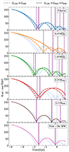 |
Fig. 1. Distance between the centre of mass of GLMC and that of GSMC. The solid (dashed) lines corresponds to the GLMC + GSMC + GMW (GLMC + GSMC) models. The different panels each represent a different set of simulations (see labels within each panel). The vertical purple solid (dashed) lines correspond to the GLMC − GSMC pericentres of the GLMC + GSMC + GMW (GLMC + GSMC) models. The vertical grey dashed line corresponds to the time we choose as the present time t = 0 (see Sect. 2.2). For the sake of comparison, in shadowed blue lines we plot the orbital history of the MCs for the models of the fiducial set. The set corresponding to a different GLMC disc mass and Toomre parameter is not shown since it shows no difference in comparison to the fiducial set. |
3.1. GSMC to GLMC distance
In Fig. 1 we show the distance between the centre of mass of the GLMC and the GSMC galaxies as a function of time. In solid lines we show the GLMC + GSMC + GMW models whereas in dashed lines we show the GLMC + GSMC. Purple vertical solid and dashed lines indicate the times of the pericentres, for each one of the models.
In the top panel, we show results from the fiducial simulations (blue lines), which are then used as guiding lines in all other panels (thin shadowed blue lines). The fiducial model shows that the time of the pericentres changes when including the gravitational pull of a GMW system. In particular, when the GMW system is present (solid lines), the pericentre is delayed for about 200 Myr. This result is a consequence of that the GSMC is initially located in between the GMW and the GLMC galaxies, and so the gravitational pull partially cancels out, and therefore the GSMC infall towards the GLMC galaxy is slower and delayed. This same effect can also be observed in all other models (see solid vs. dashed lines in all other panels). The presence of a GMW system also has an impact on the orbit of the GSMC around the GLMC galaxy. We can see that the minimum distance at pericentre is also different between the two models (with and without the GMW system). While at the first pericentre the distance is smaller when the GMW system is not present (6.2 kpc vs. 12.3 kpc), in the second the situation is reversed. This is a clear sign that the orbit has been slightly modified; that is, that the GSMC system has a different energy and angular momentum due to the gravitational pull of the GMW system. Although not analysed in this figure, this difference of the minimum distance also has a strong impact on the morphology of the GLMC galaxy disc (see Fig. 3 and Sect. 4), with the disc of the GLMC + GSMC models initially more perturbed than the one in the GLMC + GSMC + GMW.
In the second and third panels, we show the effect of changing the mass of the GLMC galaxy DM halo. First, we show that a lighter DM halo (orange lines) produces a delay on the pericentres, while a heavier DM halo (green lines) has the opposite effect. These differences have the same origin as the ones between the GLMC + GSMC + GMW and the GLMC + GSMC models (solid vs. dashed lines, respectively), that is a change on the resulting acceleration over the GSMC galaxy by the GMW and the GLMC galaxies. Like in the first panel, the variation on the pericentre time produces a change on the orbit of the GSMC system bringing it closer to the GLMC galaxy in the first pericentre when it happens earlier, i.e. the GSMC system is in a more radial orbit when the gravity of the GLMC galaxy dominates the interaction.
In the fourth panel, we show the effect of reducing the GSMC system mass (red line). We see that while the first pericentre does not change significantly from the one of the fiducial model (blue solid and dashed shadowed lines), there is a strong divergence afterwards. In particular, we see that the orbit of the GSMC system decays slower when it is lighter. This is not surprising as it is well known that the dynamical friction is more efficient for high-mass than for low-mass systems (e.g. Sect. 8.1 of Binney & Tremaine 2008; Chandrasekhar 1943).
The effect of changing the total mass and the mass distribution of the GMW system is shown in the fifth and sixth panels (dark brown and pink lines), respectively, and is similar, but with the opposite sign, to changing the mass of the GLMC galaxy DM halo. A lighter GMW system makes the gravity of the GLMC galaxy dominate the GSMC system’s infall, i.e. the first pericentre occurs earlier and the orbit is more radial (smaller GLMC − GSMC distance at pericentre), similar to the GLMC + GSMC fiducial model where GMW is not present. On the other hand, keeping the GMW system’s mass but changing its distribution to a much less realistic point-mass approximation has two effects. First, the GMW system has the same effect as if it was more massive, i.e. the pericentre is delayed with respect to the models with a lighter GMW system. This is because in the model with a GMW system with a mass distributed in a NFW profile the GLMC − GSMC system falls into the GMW DM halo long before the interaction between them starts, and therefore a non-negligible fraction of the GMW system’s mass does not contribute to the total acceleration applied to the GSMC system (i.e. Gauss theorem). This can also be deduced by the fact that the pink solid line perfectly overlaps the blue shadowed line (fiducial GLMC + GSMC + GMW model) almost down to the second pericentre when the GMW system has a close encounter with the GLMC + GSMC system, then the model significantly diverges from the fiducial. We note that considering a point-like MW also changes the dynamical friction of the interaction. Secondly, the model with a point-like GMW system all mass is pulling the GSMC in a single direction, all the time, this is the origin of the second effect we observe that is a big difference on the GSMC system’s orbit. The GSMC system experiences a strong and well directed tide by the GMW system, specially strong when it gets closer. As a consequence, the GSMC total energy-angular momentum, and therefore its orbit, highly differs from the one in other models. This can be seen by comparing the behaviour of the pink solid line just before the second pericentre and later, when the GSMC system follows a more circular orbit (larger radii and longer period between pericentres).
Finally, we note that in this figure we do not show the results from the set of models with a smaller GLMC disc mass and different Toomre parameter since the total mass of the system is the same and therefore they show no difference in the GLMC − GSMC orbital analysis with respect to the fiducial set.
3.2. Distance between the GLMC − GSMC system and GMW
Figure 2 shows the distance between the centre of mass of GLMC and that of GMW. We show that all but two of the models show no significant differences; these two are the model with a smaller GMW galaxy mass (dark brown line) and the point-like GMW model (pink line). In the former, the mutual acceleration between the GLMC galaxy and the GMW system is smaller, and so they approach each other slower (dark brown line). In the latter, although initially similar (an extended object interacts as a single-point mass when far enough), the interaction becomes stronger when the GMW system approaches the GLMC galaxy and reaches pericentre earlier (∼–0.5 Gyr), that is also when we observe large differences with the fiducial GLMC − GSMC distance (see Sect. 3.1). The variations on the GLMC − GMW distance when changing the GLMC and GSMC masses are negligible as it is the GMW system’s mass that dominates the dynamics of the GLMC − GMW interaction. Notice that, as in the previous section, we do not analyse the set of models where we changed the GLMC disc mass and Toomre parameter as these are almost identical, in total mass, to the fiducial set.
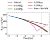 |
Fig. 2. Distance between the centre of mass of GLMC and that of GMW. Each colour represents the GLMC + GSMC + GMW model of a different set. The vertical grey dashed line corresponds to the present time t = 0. |
We also see that for the fiducial model (and most of the other models) the GMW is at a ∼200 kpc distance from the GLMC at the present time t = 0. This distance is much larger than the one obtained from observations (∼50 kpc, Pietrzyński et al. 2019). This is a result that differs from the results presented by Lucchini et al. (2021), and its origin can be in the difference in spatial and mass resolution between our models, as discussed above. For completeness, we also ran the GLMC + GSMC + GMW fiducial model for one extra Gyr to find when the GMW system gets as close to the GLMC galaxy as in the observations (i.e. 50 kpc). The result is that this happens only after the GLMC − GSMC went through three pericentres instead of the two predicted by Lucchini et al. (2021). Thus, we keep t = 0 as the snapshot after 4.0 Gyr from the initial conditions for the reasons given above.
4. The GLMC galaxy properties
4.1. t = 0 morphologies
In Fig. 3 we show the face-on (left columns) and edge-on (right columns) of the GLMC disc stellar density at t = 0 for all models2. Each row shows a different set of models (see legend in the central panels of each row). All GLMC galactic discs have been centred in the centre of mass and aligned following the procedure described in Sect. 2.3. We warn the reader that, even though it is the same instant in time for all simulations, we may not be looking at the same stage of the GLMC − GSMC interaction (see Figs. 1 and 2). In this section, we qualitatively analyse some of the features present in the stellar density map, but it is not in the scope of this paper to analyse all of them in detail. In the next sections we focus only on the bar structure.
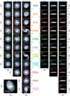 |
Fig. 3. Stellar density map of the GLMC disc as seen face-on (left part) and edge-on (right part) at t = 0. Each row corresponds to a different set of simulations and the labels are displayed in the rightmost panels. For both face-on and edge-on representations, we show the GLMC, GLMC + GSMC, and GLMC + GSMC + GMW models in the left, centre and right panels, respectively. As reference, the face-on density map of the LMC optimal sample (Jiménez-Arranz et al. 2023) is shown in the bottom left part. |
As a visual reference for the reader, we show in the left bottom part the face-on density map of the LMC optimal sample (Jiménez-Arranz et al. 2023). It is evident that two prominent overdensities are the LMC off-centred bar and the spiral arm. We first observe how the LMC spiral arm starts at the end of the bar. Then, if we analyse the spiral arm following a clockwise direction, the spiral arm breaks into two parts: an inner and an outer arm. As mentioned in Sect. 3, those are the observables we are aiming for. For the data, we have no information on the vertical component (edge-on visualisation). That is because of the lack of individual distances we need to assume that all stars lie in the z′ = 0 plane.
First, we qualitatively analyse the presence of galactic bars in our models (e.g. Hohl 1971; Noguchi 1987; Berentzen et al. 2004; Besla et al. 2012; Athanassoula et al. 2013; Yozin & Bekki 2014; Cavanagh & Bekki 2020; Bekki 2023). We see that only three models with the GLMC galaxy isolated (leftmost panels) show the presence of a bar: the fiducial model (blue panel), the model with a GLMC unstable disc (light brown panel) and the model with the GLMC with lighter DM halo (orange panel). Otherwise, we observe that the GLMC − GSMC interaction triggers the formation of bars in most models (central columns). This is specially evident in the model with the lighter GLMC disc and halo (yellow panel), the model with a GLMC stable disc (light red panel). This interaction does not only trigger the formation of a galactic bar but also can perturb the entire disc in a way that the bar ends up being off-centred (see the fiducial GLMC + GSMC + GMW simulation in the face-on top blue right panel), an observable feature of the LMC bar (e.g. Zaritsky 2004).
A second non-axisymmetric feature that is present in all our models is the spiral arms (e.g. Williams & Nelson 2001; Roca-Fàbrega et al. 2013; Michikoshi & Kokubo 2018; Sellwood & Carlberg 2019; Sellwood & Masters 2022). Most of the isolated simulations (leftmost panels) show flocculent spiral structures if they do not develop a strong bar. When a strong bar is present, the spiral arms are stronger and bisymmetric (see discussion in Roca-Fàbrega et al. 2013). In most of the simulations where the interaction with the GSMC or GMW systems occurs, we can observe both grand design (e.g. Elmegreen & Elmegreen 1982; Kendall et al. 2011) and flocculent spiral arms (e.g. Sandage 1961; Elmegreen & Elmegreen 1982; Block et al. 1996; Elmegreen et al. 2003) for different models, regardless a bar is present or not, with a variety of pitch-angles. Nonetheless, in some models we see the formation of a single grand design bisymmetric spiral arm structure also in both cases, when a bar is present and when not. For instance, in the model with lighter GLMC halo (orange right panel) and in the model with lighter GLMC disc and halo (yellow right panel) we see the formation of a high pitch-angle bisymmetric structure. Ring-like structures are also present in some models (as detected in Choi et al. 2018a), for example in the three-galaxy simulation of the model with a light GLMC disc but heavy GLMC halo (cyan right panel).
Regarding the vertical structure of GLMC, for the isolated simulations (leftmost panels) we see no noticeable asymmetries in the vertical profile beyond a small enhancement in the cases with a bar that have undergone or are undergoing a buckling event (left orange panel; e.g. Pfenniger & Friedli 1991; Łokas et al. 2014). For the interacting simulations, we observe a variety of vertical asymmetries mostly related to tidal interactions with the GSMC and GMW systems, and we also see that the disc is heated up to different degrees depending on the type of interaction.
4.2. t = 0 kinematics
Given that we possess complete information on the position and velocity of each particle, we can show the radial, residual tangential, and vertical velocity maps for the simulated GLMC galaxy disc in the same way as was possible for the LMC using Gaia DR3 data (see Jiménez-Arranz et al. 2024). The systemic motion of the centre of mass of GLMC is subtracted in order to obtain the internal velocities.
Figure 4 shows the disc radial and residual tangential velocity maps of the GLMC as seen face-on (left and right set of columns, respectively) at t = 0 for all models3. When a system is severely perturbed, as in the models with GLMC − GSMC and GLMC − GSMC − GMW interactions, a more detailed inspection is required, but we can still find systematic changes. The GLMC + GSMC + GMW simulation of the fiducial model (top blue right panels), for instance, clearly exhibits bimodality in both radial and tangential velocity. In general, the bimodality becomes more obvious when the GMW system is present (rightmost panels), which is a reflex of the effect of its tides on the GLMC disc.
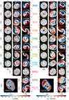 |
Fig. 4. Radial (left part) and residual tangential (right part) velocity maps of the GLMC disc as seen face-on at t = 0. Each row corresponds to a different set of simulations. For both velocity maps, we have the GLMC, GLMC + GSMC, and GLMC + GSMC + GMW models in the left, centre, and right panels, respectively. Black and white contour lines highlight the GLMC overdensities. As reference, the velocity map of the LMC optimal sample (Jiménez-Arranz et al. 2023) is shown in the bottom left part of each panel. |
The kinematic imprint of the bar can also be seen clearly in all models where a bar develops. In the radial and residual tangential velocity maps, the bar produces a quadrupole due to the elliptical orbits of the stars that form it. This is evident in the fiducial and light GLMC halo models where the GLMC is in isolation (blue and orange leftmost panels, respectively). The spiral arms also have a clear signature in the dynamics. For example, the grand design spiral arms seen in the model with lighter GLMC halo (orange right panel) and in the model with lighter GLMC disc and halo (yellow right panel) show clear signs of inwards radial migration (have a negative radial velocity).
Again, we show the radial and tangential velocity maps of the LMC optimal sample (Jiménez-Arranz et al. 2023) in the bottom left part of the corresponding panel as a visual reference for the reader. In both cases the quadrupole pattern that appears in the centre of the galaxy is related to the motion of stars in the bar. However, there is an asymmetry clearly apparent along the semi-major axis of the bar. This could be given by the inclination of the bar with respect to the disc (Besla et al. 2012). Regarding the radial velocity map, there is a negative (inward) motion along the spiral arm overdensity when this is still attached to the bar. After the break, there is no a clear trend. Regarding the residual tangential velocity map, along the spiral arm the residual tangential velocity is in general positive, that is, stars on the spiral arm move faster than the mean motion at the same radius, except for the part of the arm with a density break.
In Fig. 5 we show the GLMC disc vertical velocity maps as seen face-on at t = 0 for all models3. For the isolated simulations (leftmost panels) we observe no significant vertical velocities, as expected. However, for the interacting simulations (centre and rightmost panels), bending modes can be observed (e.g. Widrow et al. 2014; Chequers & Widrow 2017; Chequers et al. 2018). That may reflect the vertical structure seen in Fig. 3. This will be better analysed in a forthcoming paper.
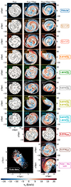 |
Fig. 5. Vertical velocity maps of the GLMC disc as seen face-on at t = 0. Each row corresponds to a different set of simulations. We show the GLMC, GLMC + GSMC, and GLMC + GSMC + GMW models in the left, centre, and right panels, respectively. Black and white contour lines highlight the GLMC overdensities. As reference, the vertical velocity map of the LMC optimal Vlos subsample (Jiménez-Arranz et al. 2023) is shown in the bottom-left corner. |
Comparing these maps with the LMC data (Jiménez-Arranz et al. 2023) is difficult because for the data there is not as much information available for the vertical velocity component. This is due to the fact that we need to know Vlos in addition to the astrometric information to determine the vertical velocity component, as seen in Sect. 3 and Appendix A of Jiménez-Arranz et al. (2023). Unfortunately, Gaia’s spectroscopic data is limited to the brightest stars, meaning that our Vlos subsamples only include tens of thousands of stars, while the full samples contain tens of millions sources. The LMC optimal Vlos subsample’s vertical velocity map is shown in the bottom left part of Fig. 5. It exhibits wave-like motion, which may be related to the warp or to the fact that dynamical equilibrium has not yet been reached by the LMC (e.g. Choi et al. 2022). Also, it may indicate that the bar is inclined with respect to the galactic plane.
5. The disc scale height of GLMC
Taking advantage that in simulations we have information of the whole temporal evolution, we can analyse how the individual GLMC − GSMC pericentres affect the GLMC disc kinematics. In particular, we show the effect of the pericentric passages on the evolution of the GLMC disc’s scale height (e.g. de Grijs & Peletier 1997; Narayan & Jog 2002a,b). In Fig. 6 we show the GLMC disc scale height hLMC as function of time for the different models. In each panel, the dotted, dashed and solid lines represent the GLMC, GLMC + GSMC and GLMC + GSMC + GMW models, respectively. In each panel, we include the isolated models as a reference point for comparison (dotted lines), and the results from the fiducial models (thin blue shadowed lines). In several models we see that the GLMC disc heating is nearly identical to the fiducial. On the other hand, we see that in models where a strong bar is present, e.g. the low GLMC halo mass model (orange dotted line), or were the GSMC system is lighter (red dotted line), the disc heating changes. In particular, for the models where a strong bar is created (low GLMC halo mass and low GLMC disc mass models, orange and light grey lines, respectively) the disc heating jumps up fast after the creation of the bar, while otherwise it remains almost negligible when interacting with a very light GSMC system (red lines).
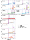 |
Fig. 6. Evolution of the scale height of the GLMC disc. The dotted, dashed, and solid lines show the GLMC, GLMC + GSMC, and GLMC + GSMC + GMW models, respectively. The different panels represent different sets of simulations. The vertical purple solid (dashed) lines correspond to the GLMC − GSMC pericentres of the GLMC + GSMC + GMW (GLMC + GSMC) models. The vertical grey dashed line corresponds to the present time t = 0. For the sake of comparison, we plot the evolution of the scale height of the GLMC disc for the models of the fiducial set in shadowed blue lines. |
The GLMC − GSMC pericentres also correlate well with a sudden increase in disc thickness, and the strength of this change correlates with the pericentre distance, the disc instability, and the merger (GSMC system) mass (e.g. Quinn et al. 1993; Moetazedian & Just 2016). The change in scale height has a peak. After the disc has heated, the thickness slightly decreases. The GLMC disc relaxes to a higher scale height than the original after the GSMC initial kick. This occurs following each GSMC system pericentre. It is clear that the change in scale height is more impulsive when the GSMC system pericentre is closer to the GLMC disc than when it occurs at greater distances, as in the case of the GLMC + GSMC + GMW simulation of the fiducial model (blue solid line) vs. the point-like MW (pink solid line) in the second pericentre (we note the pericentre distance in Fig. 1). Similar to the previous point, the simulations without GMW have a thicker GLMC galaxy disc than the simulations with a GMW system, for all models. This might result from the first passages being closer together than they would be in the absence of the GMW system. If the mass of the GLMC disc is smaller (right panels), the results do not change significantly for the fiducial and heavy LMC halo (grey and cyan lines, respectively) but they do for the light GLMC halo (yellow lines).
6. The GLMC bar
In this section we aim to study the evolution of the GLMC galaxy bar properties in a quantitative way, including the bar strength, length and pattern speed (e.g. Tremaine & Weinberg 1984; Athanassoula 1992; Debattista & Sellwood 2000; Sellwood 2014; Cuomo et al. 2019; Guo et al. 2019; Géron et al. 2023; Buttitta et al. 2023) when in isolation and when interacting with the GSMC and GMW systems.
To this end, we applied the Dehnen method to the GLMC disc for all available snapshots and for all simulations. The Dehnen method (Dehnen et al. 2023) measures the bar pattern speed Ωp and the orientation angle ϕb of the bar from single snapshots of simulated barred galaxies. The method also determines the bar region, defined by the inner and outer radius [R0, R1]. Hereafter we will refer to R1 as the bar radius or length, as it agrees well with the definition of best estimates for bar lengths in numerical simulations (Ghosh & Di Matteo 2024). For more details about the method see Sect. 2 and Appendix B of Dehnen et al. (2023).
6.1. The GLMC bar strength
In Fig. 7, we show the median relative m = 2 Fourier amplitude Σ2/Σ0 in the bar region given by the inner and outer radius [R0, R1] as function of time. Since the GLMC galaxy disc is relaxing at the beginning of the simulation, we choose not to display the evolution of the disc in the first 1.25 Gyr, which corresponds to two times the disc rotation. Again, in each panel, the dotted, dashed and solid lines represent the GLMC, GLMC + GSMC and GLMC + GSMC + GMW configurations, respectively. To consider that the disc shows a bar, we impose a threshold of Σ2/Σ0 > 0.2 (as in Fujii et al. 2019; Bland-Hawthorn et al. 2023). As qualitatively seen in Fig. 3, when the GLMC galaxy is in isolation only three models make the disc unstable enough to form a bar; the fiducial model, the GLMC unstable disc model and the GLMC with lighter DM halo model, corresponding to the blue, light brown and orange dotted lines, respectively.
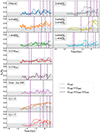 |
Fig. 7. Same as Fig. 6 but for the relative m = 2 Fourier amplitude of the GLMC bar region. The grey area corresponds to Σ2/Σ0 = 0.2, which is the threshold used to consider whether or not the GLMC disc has a bar. The first 1.25 Gyr are not shown because this is when the GLMC disc is being relaxed, which corresponds to two times the disc rotation. |
In the fiducial model, if the GSMC is present (blue dashed line), we observe how the bar strength is increased ∼0.5 Gyr after the first pericentre and from then, it oscillates. If both GSMC and GMW are present (blue solid line), the amplitude of the bar formed is very near the threshold value showing a weak bar.
Analysing the consequences of having a light or heavy GLMC halo mass on the GLMC bar strength, we observe how reducing the GLMC halo mass (orange lines) makes the disc less stable, allowing it to form a stronger bar in comparison to the fiducial model, for all configurations. The GLMC + GSMC + GMW configuration can produce a bar up to Σ2/Σ0 = 0.4 for the present time t = 0. On the contrary, increasing the GLMC halo mass (green lines) makes the disc more stable, making it more difficult to form a bar in comparison to the fiducial model, for all configurations. This is in agreement with simulations in the literature (e.g. Roca-Fàbrega et al. 2013).
Regarding the models where the mass of the GLMC disc is smaller (right panels), if we compare all the models of different GLMC halo mass (grey, yellow and cyan lines) with their analogue models with a heavier GLMC disc (blue, orange and green lines, on their left, respectively), we observe that the amplitude of the bar is larger in all cases. This is caused by the fact that, despite being more internally stable, the GLMC disc is more sensitive to external perturbations because the stellar particles are less gravitationally bound.
In the models where the GSMC is lighter (red lines), the GMW mass is smaller (dark brown line) and the GMW is considered point-like (pink like), the GLMC shows no bar formation, with differences far from the stochastic variation of the second order Fourier mode with respect to the fiducial model.
The change of the Toomre parameter Q, i.e. the gravitational stability of the stellar disc, has a significant impact on the bar formation for the isolated GLMC models, as expected. The more unstable the disc is (light brown dotted line), the stronger the bar is, independently of whether there is or not interaction with other galactic systems. However, for the GLMC + GSMC model, we observe how the bar strength decreases after the second GLMC − GSMC pericentre, being the value close to the threshold of Σ2/Σ0 = 0.2 at t = 0. Otherwise, in a more stable disc (light red dotted line), bars are not formed by secular evolution, but we observe how the first GLMC − GSMC pericentre boosts the formation of a strong bar on the GLMC galaxy 0.5 − 1 Gyr after the interaction, for both interacting models.
6.2. The GLMC bar length
In Fig. 8 we show the outer bar region R1 of GLMC given by the Dehnen method as function of time, when the relative m = 2 Fourier amplitude Σ2/Σ0 is above the 0.2 threshold value. Here and hereafter, the crosses, the empty circles and the filled circles represent the GLMC, GLMC + GSMC and GLMC + GSMC + GMW configurations, respectively. From the three bars created in isolation (fiducial, low mass GLMC galaxy halo and unstable GLMC disc, represented by the blue, orange and light brown crosses, respectively) the longest is the low mass GLMC galaxy halo model. The horizontal green area corresponds to the LMC bar length measured in Jiménez-Arranz et al. (2024), R1, LMC = 2.3 kpc. As happens in the fiducial model, both bars grow over time by a factor ∼2 when comparing the end of the simulations with the time when the bar is formed. On the other hand, the model with unstable GLMC disc has a constant bar length R1, LMC ∼ 2.5 kpc over time.
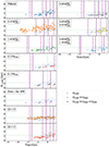 |
Fig. 8. Evolution of the GLMC bar length given by the outer bar radius R1 from the Dehnen method. The cross corresponds to the isolated GLMC model, whereas the empty and filled dots show the GLMC + GSMC and GLMC + GSMC + GMW models, respectively. The different panels represent different sets of simulations. The vertical purple solid (dashed) lines correspond to the pericentres of the MCs of the GLMC + GSMC + GMW (GLMC + GSMC) models. The vertical grey dashed line corresponds to the present time t = 0. The horizontal green area corresponds to the LMC bar length measured in Jiménez-Arranz et al. (2024), R1, LMC = 2.3 kpc. For the sake of comparison, the evolution of the GLMC bar length for the models of the fiducial set is plotted in shadowed blue lines. We only show the obtained value when Σ2/Σ0 > 0.2, which is the threshold used to consider that the GLMC disc has a bar. |
We see very complex behaviours on the GLMC bar length for the interacting configurations (empty and filled circles). The shortest bars are of ≲1 kpc length and are obtained for interacting models with and without the GMW (see, for example, the grey and green circles). The largest bars are created in the lighter GLMC halo model (orange circles) with a length of ≳5 kpc. Whereas for some models the GLMC − GSMC pericentres imply a change in the bar length, as for example in the fiducial and heavy GLMC DM halo model (blue and green crosses and circles, respectively), for other models the interaction does not have an impact on the GLMC bar length change, as in the unstable GLMC disc model (light brown crosses and circles).
6.3. Analysis of the GLMC bar off-centredness
Besla et al. (2012) demonstrated that the off-centre stellar bar of the LMC (and its one-armed spiral) can be naturally explained by a recent direct collision with the SMC. Here we analyse how the interaction of the GSMC with the GLMC can affect the position of the centre of the stellar bar of the GLMC.
Figure 9 shows the analysis of how off-centred the bar of the GLMC is, determined by the distance between the GLMC centre of mass and its bar centre (obtained using a KDE of 3.0 kpc-bandwidth, as explained in Sect. 2.3), when the relative m = 2 Fourier amplitude Σ2/Σ0 is above the 0.2 threshold value. The three bars created in isolation (fiducial, low mass GLMC galaxy halo and unstable GLMC disc, represented by the blue, orange and light brown crosses, respectively) share their centre with the centre of mass, as expected, leading to an ∼0 kpc bar off-centre.
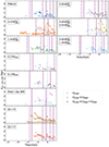 |
Fig. 9. Same as Fig. 8 but for the GLMC off-centre bar. The evolution of the GLMC bar off-centredness is given by the distance between the centre of mass of GLMC and the GLMC bar centre obtained using a KDE of 3.0 kpc bandwidth as explained in Sect. 2.3. |
We observe how the GLMC − GSMC pericentres in the interacting models produce an increase in the bar off-centre. In the full configurations of the light GLMC halo (orange filled circles) and the light GLMC disc and halo (yellow filled circles) models are where the increased bar off-centre is more readily apparent (up to ∼2 − 3 kpc) ∼0.5 Gyr after the first pericentre and from then, it decreases where the bar tries to be located at the centre of mass of the host galaxy. In the majority of simulations we observe an off-centre bar at a certain point of the temporal evolution.
6.4. The GLMC bar pattern speed
Figure 10 shows the GLMC bar pattern speed Ωp given by the Dehnen method as function of time, when the relative m = 2 Fourier amplitude Σ2/Σ0 is above the 0.2 threshold value. The horizontal green area corresponds to the LMC bar pattern speed measured in Jiménez-Arranz et al. (2024) using the bisymmetric velocity (BV) method (Gaia Collaboration 2023),  km s−1 kpc−1. The three bars created in the isolated configuration (fiducial, low mass GLMC galaxy halo and unstable GLMC disc, represented by the blue, orange and light brown crosses, respectively) slow down over time (e.g. Athanassoula 2003; Widrow et al. 2008). In comparison to the fiducial model, the low mass GLMC halo presents a stronger and slower bar, whereas the unstable GLMC disc has a even stronger bar that roughly rotates at the same angular speed.
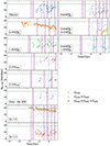 |
Fig. 10. Same as Fig. 8 but for the GLMC bar pattern speed. The horizontal green area corresponds to the LMC bar pattern speed measured in Jiménez-Arranz et al. (2024) using the bisymmetric velocity method (Gaia Collaboration 2023), |
As in the case of the bar length, we see very complex behaviours for the interacting configurations (empty and filled circles). For the fiducial model, the interacting configurations have bars with smaller pattern speeds than in the isolated configuration. For the interacting configurations corresponding to the two models with more unstable discs (low mass GLMC halo and GLMC disc Q = 1.0 models, represented by orange and light brown empty and filled circles, respectively) we do not observe significant differences with respect to the decreasing pattern speed shown by the isolated models (crosses). For t > 0, the GLMC + GSMC models show a bar ∼5 km s−1 slower (faster) for the low mass GLMC halo (Q = 1.0) models in comparison to the isolated model.
7. Summary and discussion
In this paper, we present KRATOS, a comprehensive suite of 28 pure N-body simulations of isolated and interacting LMC-like and SMC-mass galaxies. The 28 simulations are grouped into 11 sets of up to three simulations, including: (1) a control model with an isolated LMC-like galactic system; (2) a model with both an LMC-like and a SMC-mass system; and (3) a model that contains both an LMC-like and a SMC-mass system and an MW-mass system in addition. For each of the three model combinations, or scenarios, we vary a set of the free parameters of the whole system (details given in Sect. 2). The simulations have a spatial and temporal resolution of 10 pc and 5000 yr, respectively. The minimum mass per particle is 4 × 10³ M⊙.
The KRATOS suite is devoted to the analysis of the formation of substructures in an LMC-like disc after the interaction with an SMC-mass system and to the comparison of these formations with observations (see e.g. the kinematics maps of the LMC using Gaia data in Gaia Collaboration 2021b; Jiménez-Arranz et al. 2023). The majority of simulations in the literature on the interaction between the LMC, SMC, and MW have so far been carried out to analyse and recreate the distribution and position of the gas components of these systems, such as the Magellanic Corona, the Leading Arm, and Magellanic Stream (Besla et al. 2010, 2012; Hammer et al. 2015; Pardy et al. 2018; Wang et al. 2019; Tepper-García et al. 2019; Lucchini et al. 2020, 2021). Besla et al. (2012) have been the only authors to extensively explore the effect of this interaction on the internal structures of the LMC; namely the off-centre bar and the single spiral arm. It may be possible to learn more about the interactions that took place between these two satellite galaxies and between them and the MW by exploring the formation process of these LMC morphological features.
For the fiducial model of the KRATOS suite, we determined that it is more crucial for the GLMC and GSMC systems to have completed two pericentres internally than for the distance to the GMW to match observations. Mutual interactions between GLMC and GSMC are far more significant than the interaction with the GMW (e.g. de Vaucouleurs & Freeman 1972; Besla et al. 2012), because tidal effects are smaller at greater distances, even if the Milky Way is more massive. Although at present time the GLMC and GSMC are not as close to the GMW as one would like they are nevertheless useful illustrations of the interaction between these two MW neighbours, and models of these interactions can be contrasted with observations.
In Table 3, we compare the initial conditions of the fiducial model of the KRATOS suite and the models presented in Besla et al. (2012, hereafter B12). The B12 models include hydrodynamics, whereas the KRATOS suite contains pure N-body simulations. Differences can be found in both the amount of mass of the three galaxies and how it is distributed. For instance, in B12, the LMC is modelled with a disc of gas and a disc of stars surrounded by a DM halo with a Hernquist profile, whereas in KRATOS the LMC is modelled as a disc of stars surrounded by a NFW DM halo. A significant difference lies on the modelling of the MW, where B12 models the Galaxy as a static NFW potential, whereas KRATOS simulates the MW as a live NFW DM halo. However, the authors of B12 claim that not considering dynamical friction from the MW halo is expected to have little impact on the orbit in a first passage scenario. Conversely, in both works, the effect of modelling the LMC and SMC as an isolated binary pair or in interaction with the MW potential is analysed. Finally, in terms of the resolution of B12 and KRATOS, the two simulations have of the order of ∼106 star particles in the GLMC disc, but there are many more particles in the GLMC DM halo in the KRATOS simulations than in B12 (10 − 35 vs 0.1 × 10⁶). For GSMC, KRATOS exhibits fewer star particles (0.6 vs 1 × 10⁵) but a significantly larger number of DM particles (0.01 vs 1 − 4.5 × 10⁶). The minimum mass per particle is 2.5 × 10³ M⊙ for B12 and 4 × 10³ M⊙ for KRATOS. The spatial resolutions of B12 and KRATOS are 100 and 10 pc, respectively. In Besla et al. (2012), no explicit information is given on the temporal resolution of B12, while it is of 5000 yr for KRATOS.
Comparison of the initial conditions of the GLMC, GSMC, and GMW galaxies for the fiducial model presented in this work (KRATOS) and the model presented by Besla et al. (2012, B12).
It is possible to compare – accounting for the differences between works – the structure of the LMC stellar disc after the two encounters with the SMC galaxy using both the KRATOS and B12 simulations. As a result of the direct collision between the SMC and the LMC in Model 2 of B12, the LMC bar is off-centre relative to the disc shortly after the pericentre of the two galaxies. The same outcome is shown in our Fig. 9, where the off-centredness of the bar is caused by the tidal interaction between the GLMC and GSMC. In B12, the result of this last interaction is a warping of the LMC bar by approximately ∼10° −15° with respect to the LMC disc plane. Further analysis of this situation is deferred to future work on the KRATOS suite. Regarding the formation of a single bar, both B12 (see their Fig. 11, right panel) and KRATOS (our Fig. 3) recover this characteristic morphological feature of the LMC. Finally, as our simulations are pure N-body, we are unable to compare the gas component of either galaxy with those found in the B12 models.
The KRATOS simulations offer a variety of galaxy formation and evolution, in the sense that GLMC are isolated galaxies, while in GLMC − GSMC and GLMC − GSMC − GMW the GLMC is interacting with the GSMC or with both GSMC and GMW. Under these different scenarios, we can compare the bar fraction in the suite of 28 simulations in KRATOS with that of nearby galaxies, taking into account that they also have different formation histories. In the KRATOS suite, we quantify the number of bars (as used in this work, with Σ2/Σ0 amplitude larger than 20%). We find that in 17 out of the 28 simulations, the disc develops either a weak and transient (less than 1.5 Gyr approx.) or strong bar. Only 11 of the models do not show a clear bar in any moment of the evolution of the galaxy. These numbers agree with the fraction of bars observed in nearby galaxies (e.g. Marinova et al. 2007; Menéndez-Delmestre et al. 2007; Barazza et al. 2008; Sheth et al. 2008; Nair & Abraham 2010; Masters et al. 2011), which is about 30%–60%. Out of the barred galaxy models, 6 show a weak (below 20% or very transient in time bar structure), while 11 models show a strong and long-lived bar (more than 1.5 Gyr). These strong bars may have different origin: 3 of them lie in the control GLMC models so they develop as internal disc instabilities; 4 of them are formed in models with GLMC and GSMC interaction or even with GMW interaction. While 4 bars form in models of interacting galaxies, but the corresponding control GLMC also develops a bar, so both mechanisms could create the bar structure.
As mentioned above, KRATOS simulations are designed to compare with the internal LMC disc kinematics (e.g. Gaia Collaboration 2021b; Jiménez-Arranz et al. 2023). In Jiménez-Arranz et al. (2024), the LMC bar pattern speed is studied using Gaia DR3 data. In this previous work, we use three different methods to evaluate the bar properties: the bar pattern speed is measured through the Tremaine-Weinberg (TW, Tremaine & Weinberg 1984) method, the Dehnen method (introduced in our Sect. 2.3) and a bisymmetric velocity (BV) model (Gaia Collaboration 2023). The work suggests that due to the significant variation with frame orientation, the TW method appears to be unable to determine which global value best represents an LMC bar pattern speed. The Dehnen method gives a pattern speed of Ωp = −1.0 ± 0.5 km s−1 kpc−1, corresponding to a bar that barely rotates, and is slightly counter-rotating with respect to the LMC disc. This method does not take into account a possible strong and counter-rotating m = 1 disc component, which would balance the bar pattern speed. The BV method recovers a LMC bar corotation radius of Rc = 4.20 ± 0.25 kpc, corresponding to a pattern speed  km s−1 kpc−1 (horizontal green area of Fig. 10). This result is consistent with previous estimates and gives a bar corotation-to-length ratio of Rc/Rbar = 1.8 ± 0.1, which makes the LMC hosting a slow bar, as most interacting bars found in nearby galaxies (e.g. Géron et al. 2023). The pattern speed of the bars in the KRATOS simulations also fall within this range of Ωp = 10 − 20 km s−1 kpc−1, suggesting indeed that the LMC has a slow rotating bar.
Regarding the disc scale height computed in the KRATOS simulations and comparing to recent values in the literature, Ripepi et al. (2022) find, using classical cepheids, that the LMC disc appears ‘flared’ and thick, with a disc scale height of hLMC = 0.97 kpc. The authors argued that strong tidal interactions with the MW and/or SMC, as well as previous mergers involving now-disrupted LMC satellites, can all be used to explain this feature. Since the present scale height is sensitive to the initial conditions of the GLMC disc, we do not aim to replicate it in our paper. However, we state that interactions indeed lead to a significant increase in the GLMC thickness.
8. Conclusions
In this paper, we introduce a comprehensive suite of 28 pure N-body and open access simulations named KRATOS with our goal being to study the internal kinematics of the LMC disc. Gaia DR3 contains complex and rich velocity maps (e.g. Gaia Collaboration 2021b; Jiménez-Arranz et al. 2023). The interpretation of these maps requires a range of simulated LMC models. In this work, we generate models with three different configurations: a control GLMC as an isolated LMC galaxy, another configuration with the GSMC only interaction, and finally the most realistic situation where both the GSMC and GMW may interact with the GLMC. We take into account the uncertainties regarding structural parameters and orbital parameters by considering a different set of initial conditions, where we vary one of the parameters at a time (see Table 2).
Results shown in this paper from the KRATOS suite can be summarised as follows:
-
Regarding the orbital history between the GLMC and the GSMC, the outcome of not including the GMW is that the pericentric passages between the two galaxies happen earlier than when the three galaxies are present (see Fig. 1).
-
In relation to the orbital history between the GMW and the GLMC, the higher the mass of the GMW, the closer the two galaxies will become, as expected (see Fig. 2).
-
The KRATOS simulations are suited to exploring different GLMC galaxy morphologies, as a large variety of spiral arm shapes can be investigated, as well as the presence of a bar, warped discs, and so on, as seen in Fig. 3.
-
Different galaxy morphologies also translate into different kinematic maps of the disc, and these can be used to help us make a first interpretation of the LMC kinematic maps (e.g. Gaia Collaboration 2021b; Jiménez-Arranz et al. 2023), as seen in Figs. 4 and 5.
-
As Cepheids suggest (Ripepi et al. 2022), the GLMC disc scale height is increased just after a pericentric passage of the GSMC as seen in Fig. 6 for all models.
-
Tidal interactions cannot only destroy bars (when they are formed), but can also create them, as seen in Fig. 7.
-
As also seen by Besla et al. (2012), we observe that the off-centre stellar bar of the GLMC can be naturally explained by a recent direct interaction with the GSMC, as seen in Figs. 3 and 9.
-
The GSMC pericentric passages do not significantly change the length and pattern speed of long-lived bars, as seen in Figs. 8 and 10.
-
As suggested by Géron et al. (2023), the longest bars are the ones with the lowest pattern speeds (see their Fig. 12.).
In summary, the KRATOS suite of N-body simulations is designed to be used to study the internal kinematics of the GLMC disc and to help in the interpretation of the complex maps obtained from Gaia data. The high spatial, temporal, and mass resolutions used in the simulations prove to be beneficial for this endeavour, as shown by the preliminary scientific results presented in this work. A more detailed analysis of the LMC–SMC interaction is left for the subsequent papers of this series.
Movies
Movie 1 associated (macroplot_velocity_vertical) Access Supplementary Material
Movie 2 associated (macroplot_velocity_radial_residual_tangential) Access Supplementary Material
Movie 3 associated (macroplot_density) Access Supplementary Material
The simulations are open access. Readers interested in using the simulations developed in the paper can access them at https://dataverse.csuc.cat/dataset.xhtml?persistentId=doi:10.34810/data1156.
The animation showcasing the evolutionary changes in the face-on and edge-on distributions throughout the entire simulation is available online.
The animation showcasing the evolutionary changes in the radial, residual tangential and vertical distribution throughout the entire simulation is available online.
Acknowledgments
We thank an anonymous referee for a critical review and constructive suggestions that helped improving the manuscript. This work was (partially) supported by the Spanish MICIN/AEI/10.13039/501100011033 and by “ERDF A way of making Europe” by the “European Union” through grants PID2021-122842OB-C21 and PID2021-125451NA-I00, the European Union “Next Generation EU”/PRTR through grant CNS2022-135232, and the Institute of Cosmos Sciences University of Barcelona (ICCUB, Unidad de Excelencia ‘María de Maeztu’) through grant CEX2019-000918-M. OJA acknowledges funding by l’Agència de Gestió d’Ajuts Universitaris i de Recerca (AGAUR) official doctoral program for the development of a R+D+i project under the FI-SDUR grant (2020 FISDU 00011). SRF acknowledges support from the Knut and Alice Wallenberg Foundation, and from the Swedish Research Council (grant 2019-04659). He also acknowledges support from the Spanish Ministry of Science and Innovation through projects PID2020-114581GB-C22 and PID2022-138896NB-C55. MB acknowledges funding from the University of Barcelona’s official doctoral program for the development of a R+D+i project under the PREDOCS-UB grant. PM gratefully acknowledges support from project grants from the Swedish Research Council (Vetenskaprådet, Reg: 2017-03721; 2021-04153). LC acknowledges financial support from the Chilean Agencia Nacional de Investigación y Desarrollo (ANID) through the Fondo Nacional de Desarrollo Científico y Tecnológico (FONDECYT) Regular Project 1210992. This work was partially supported by the OCRE awarded project Galactic Research in Cloud Services (Galactic RainCloudS). OCRE receives funding from the European Union’s Horizon 2020 research and innovation programme under grant agreement no. 824079.
References
- Almeida, A., Anderson, S. F., Argudo-Fernández, M., et al. 2023, ApJS, 267, 44 [NASA ADS] [CrossRef] [Google Scholar]
- Amiaux, J., Scaramella, R., Mellier, Y., et al. 2012, SPIE Conf. Ser., 8442, 84420Z [NASA ADS] [Google Scholar]
- Athanassoula, E. 1992, MNRAS, 259, 345 [Google Scholar]
- Athanassoula, E. 2003, MNRAS, 341, 1179 [Google Scholar]
- Athanassoula, E., Machado, R. E. G., & Rodionov, S. A. 2013, MNRAS, 429, 1949 [Google Scholar]
- Bagheri, G., Cioni, M. R. L., & Napiwotzki, R. 2013, A&A, 551, A78 [NASA ADS] [CrossRef] [EDP Sciences] [Google Scholar]
- Barazza, F. D., Jogee, S., & Marinova, I. 2008, ApJ, 675, 1194 [Google Scholar]
- Bekki, K. 2023, MNRAS, 523, 5823 [NASA ADS] [CrossRef] [Google Scholar]
- Berentzen, I., Athanassoula, E., Heller, C. H., & Fricke, K. J. 2004, MNRAS, 347, 220 [Google Scholar]
- Besla, G., Kallivayalil, N., Hernquist, L., et al. 2007, ApJ, 668, 949 [Google Scholar]
- Besla, G., Kallivayalil, N., Hernquist, L., et al. 2010, ApJ, 721, L97 [Google Scholar]
- Besla, G., Kallivayalil, N., Hernquist, L., et al. 2012, MNRAS, 421, 2109 [Google Scholar]
- Binney, J., & Tremaine, S. 2008, Galactic Dynamics: Second Edition (Princeton, USA: Princeton University Press) [Google Scholar]
- Bland-Hawthorn, J., Tepper-Garcia, T., Agertz, O., & Freeman, K. 2023, ApJ, 947, 80 [NASA ADS] [CrossRef] [Google Scholar]
- Block, D. L., Elmegreen, B. G., & Wainscoat, R. J. 1996, Nature, 381, 674 [NASA ADS] [CrossRef] [Google Scholar]
- Buttitta, C., Corsini, E. M., Aguerri, J. A. L., et al. 2023, MNRAS, 521, 2227 [NASA ADS] [CrossRef] [Google Scholar]
- Carrera, R., Conn, B. C., Noël, N. E. D., Read, J. I., & López Sánchez, Á. R. 2017, MNRAS, 471, 4571 [Google Scholar]
- Cavanagh, M. K., & Bekki, K. 2020, A&A, 641, A77 [NASA ADS] [CrossRef] [EDP Sciences] [Google Scholar]
- Chandrasekhar, S. 1943, ApJ, 97, 255 [Google Scholar]
- Chequers, M. H., & Widrow, L. M. 2017, MNRAS, 472, 2751 [NASA ADS] [CrossRef] [Google Scholar]
- Chequers, M. H., Widrow, L. M., & Darling, K. 2018, MNRAS, 480, 4244 [CrossRef] [Google Scholar]
- Choi, Y., Nidever, D. L., Olsen, K., et al. 2018a, ApJ, 869, 125 [Google Scholar]
- Choi, Y., Nidever, D. L., Olsen, K., et al. 2018b, ApJ, 866, 90 [Google Scholar]
- Choi, Y., Olsen, K. A. G., Besla, G., et al. 2022, ApJ, 927, 153 [NASA ADS] [CrossRef] [Google Scholar]
- Choudhury, S., Subramaniam, A., Cole, A. A., & Sohn, Y. J. 2018, MNRAS, 475, 4279 [NASA ADS] [CrossRef] [Google Scholar]
- Cioni, M. R. L., van der Marel, R. P., Loup, C., & Habing, H. J. 2000, A&A, 359, 601 [Google Scholar]
- Cioni, M. R. L., Clementini, G., Girardi, L., et al. 2011, A&A, 527, A116 [CrossRef] [EDP Sciences] [Google Scholar]
- Cuomo, V., Lopez Aguerri, J. A., Corsini, E. M., et al. 2019, A&A, 632, A51 [NASA ADS] [CrossRef] [EDP Sciences] [Google Scholar]
- de Grijs, R., & Peletier, R. F. 1997, A&A, 320, L21 [NASA ADS] [Google Scholar]
- de Jong, R. S., Agertz, O., Berbel, A. A., et al. 2019, The Messenger, 175, 3 [NASA ADS] [Google Scholar]
- de Vaucouleurs, G., & Freeman, K. C. 1972, Vistas Astron., 14, 163 [Google Scholar]
- Debattista, V. P., & Sellwood, J. A. 2000, ApJ, 543, 704 [Google Scholar]
- Dehnen, W., Semczuk, M., & Schönrich, R. 2023, MNRAS, 518, 2712 [Google Scholar]
- Diaz, J. D., & Bekki, K. 2012, ApJ, 750, 36 [Google Scholar]
- Duffy, A. R., Schaye, J., Kay, S. T., et al. 2010, MNRAS, 405, 2161 [NASA ADS] [Google Scholar]
- Elmegreen, D. M., & Elmegreen, B. G. 1980, AJ, 85, 1325 [NASA ADS] [CrossRef] [Google Scholar]
- Elmegreen, D. M., & Elmegreen, B. G. 1982, MNRAS, 201, 1021 [NASA ADS] [CrossRef] [Google Scholar]
- Elmegreen, B. G., Leitner, S. N., Elmegreen, D. M., & Cuillandre, J.-C. 2003, ApJ, 593, 333 [NASA ADS] [CrossRef] [Google Scholar]
- Euclid Collaboration (Scaramella, R., et al.) 2022, A&A, 662, A112 [NASA ADS] [CrossRef] [EDP Sciences] [Google Scholar]
- Fathi, K., Allen, M., Boch, T., Hatziminaoglou, E., & Peletier, R. F. 2010, MNRAS, 406, 1595 [NASA ADS] [Google Scholar]
- Fujii, M. S., Bédorf, J., Baba, J., & Portegies Zwart, S. 2019, MNRAS, 482, 1983 [NASA ADS] [CrossRef] [Google Scholar]
- Gaia Collaboration (Prusti, T., et al.) 2016, A&A, 595, A1 [NASA ADS] [CrossRef] [EDP Sciences] [Google Scholar]
- Gaia Collaboration (Brown, A. G. A., et al.) 2021a, A&A, 649, A1 [NASA ADS] [CrossRef] [EDP Sciences] [Google Scholar]
- Gaia Collaboration (Luri, X., et al.) 2021b, A&A, 649, A7 [EDP Sciences] [Google Scholar]
- Gaia Collaboration (Drimmel, R., et al.) 2023, A&A, 674, A37 [CrossRef] [EDP Sciences] [Google Scholar]
- Gallagher, I., J. S., & Hunter, D. A. 1984, ARA&A, 22, 37 [NASA ADS] [CrossRef] [Google Scholar]
- Garavito-Camargo, N., Besla, G., Laporte, C. F. P., et al. 2019, ApJ, 884, 51 [NASA ADS] [CrossRef] [Google Scholar]
- Gardiner, L. T., & Noguchi, M. 1996, MNRAS, 278, 191 [Google Scholar]
- Gardiner, L. T., Sawa, T., & Fujimoto, M. 1994, MNRAS, 266, 567 [NASA ADS] [CrossRef] [Google Scholar]
- Géron, T., Smethurst, R. J., Lintott, C., et al. 2023, MNRAS, 521, 1775 [CrossRef] [Google Scholar]
- Ghosh, S., & Di Matteo, P. 2024, A&A, 683, A100 [NASA ADS] [CrossRef] [EDP Sciences] [Google Scholar]
- Graczyk, D., Pietrzyński, G., Thompson, I. B., et al. 2014, ApJ, 780, 59 [Google Scholar]
- Grady, J., Belokurov, V., & Evans, N. W. 2021, ApJ, 909, 150 [Google Scholar]
- Guo, R., Mao, S., Athanassoula, E., et al. 2019, MNRAS, 482, 1733 [Google Scholar]
- Hammer, F., Yang, Y. B., Flores, H., Puech, M., & Fouquet, S. 2015, ApJ, 813, 110 [NASA ADS] [CrossRef] [Google Scholar]
- Harris, J. 2007, ApJ, 658, 345 [Google Scholar]
- Hilditch, R. W., Howarth, I. D., & Harries, T. J. 2005, MNRAS, 357, 304 [NASA ADS] [CrossRef] [Google Scholar]
- Hindman, J. V., Kerr, F. J., & McGee, R. X. 1963, Aust. J. Phys., 16, 570 [Google Scholar]
- Hohl, F. 1971, ApJ, 168, 343 [NASA ADS] [CrossRef] [Google Scholar]
- Irwin, M. J., Kunkel, W. E., & Demers, S. 1985, Nature, 318, 160 [Google Scholar]
- Ivezić, Ž., Kahn, S. M., Tyson, J. A., et al. 2019, ApJ, 873, 111 [Google Scholar]
- Jiao, Y., Hammer, F., Wang, H., Wang, J., & Yang, Y. 2023, arXiv e-prints [arXiv:2306.05461] [Google Scholar]
- Jiménez-Arranz, Ó., Romero-Gómez, M., Luri, X., et al. 2023, A&A, 669, A91 [NASA ADS] [CrossRef] [EDP Sciences] [Google Scholar]
- Jiménez-Arranz, Ó., Chemin, L., Romero-Gómez, M., et al. 2024, A&A, 683, A102 [NASA ADS] [CrossRef] [EDP Sciences] [Google Scholar]
- Kallivayalil, N., van der Marel, R. P., & Alcock, C. 2006a, ApJ, 652, 1213 [NASA ADS] [CrossRef] [Google Scholar]
- Kallivayalil, N., van der Marel, R. P., Alcock, C., et al. 2006b, ApJ, 638, 772 [NASA ADS] [CrossRef] [Google Scholar]
- Kallivayalil, N., van der Marel, R. P., Besla, G., Anderson, J., & Alcock, C. 2013, ApJ, 764, 161 [Google Scholar]
- Kendall, S., Kennicutt, R. C., & Clarke, C. 2011, MNRAS, 414, 538 [NASA ADS] [CrossRef] [Google Scholar]
- Kerr, F. J., Hindman, J. F., & Robinson, B. J. 1954, Aust. J. Phys., 7, 297 [NASA ADS] [CrossRef] [Google Scholar]
- Kim, S., Staveley-Smith, L., Dopita, M. A., et al. 1998, ApJ, 503, 674 [Google Scholar]
- Kollmeier, J., Anderson, S. F., Blanc, G. A., et al. 2019, Bull. Am. Astron. Soc., 51, 274 [Google Scholar]
- Kravtsov, A. V., Klypin, A. A., & Khokhlov, A. M. 1997, ApJS, 111, 73 [Google Scholar]
- Lilley, E. J., Evans, N. W., & Sanders, J. L. 2018, MNRAS, 476, 2086 [NASA ADS] [CrossRef] [Google Scholar]
- Lin, D. N. C., & Lynden-Bell, D. 1982, MNRAS, 198, 707 [NASA ADS] [CrossRef] [Google Scholar]
- Łokas, E. L., Athanassoula, E., Debattista, V. P., et al. 2014, MNRAS, 445, 1339 [Google Scholar]
- Lucchini, S., D’Onghia, E., Fox, A. J., et al. 2020, Nature, 585, 203 [CrossRef] [Google Scholar]
- Lucchini, S., D’Onghia, E., & Fox, A. J. 2021, ApJ, 921, L36 [NASA ADS] [CrossRef] [Google Scholar]
- Luks, T., & Rohlfs, K. 1992, A&A, 263, 41 [NASA ADS] [Google Scholar]
- Marinova, I., Jogee, S., Bacon, D., et al. 2007, Am Astron. Soc. Meeting Abstr., 211, 97.12 [NASA ADS] [Google Scholar]
- Masters, K. L., Nichol, R. C., Hoyle, B., et al. 2011, MNRAS, 411, 2026 [Google Scholar]
- Menéndez-Delmestre, K., Sheth, K., Schinnerer, E., Jarrett, T. H., & Scoville, N. Z. 2007, ApJ, 657, 790 [Google Scholar]
- Michikoshi, S., & Kokubo, E. 2018, MNRAS, 481, 185 [NASA ADS] [CrossRef] [Google Scholar]
- Misawa, T., Charlton, J. C., Kobulnicky, H. A., Wakker, B. P., & Bland-Hawthorn, J. 2009, ApJ, 695, 1382 [NASA ADS] [CrossRef] [Google Scholar]
- Moetazedian, R., & Just, A. 2016, MNRAS, 459, 2905 [NASA ADS] [CrossRef] [Google Scholar]
- Murai, T., & Fujimoto, M. 1980, PASJ, 32, 581 [NASA ADS] [Google Scholar]
- Nair, P. B., & Abraham, R. G. 2010, ApJ, 714, L260 [Google Scholar]
- Narayan, C. A., & Jog, C. J. 2002a, A&A, 390, L35 [NASA ADS] [CrossRef] [EDP Sciences] [Google Scholar]
- Narayan, C. A., & Jog, C. J. 2002b, A&A, 394, 89 [NASA ADS] [CrossRef] [EDP Sciences] [Google Scholar]
- Navarro, J. F., Frenk, C. S., & White, S. D. M. 1996, ApJ, 462, 563 [Google Scholar]
- Nidever, D. L., Majewski, S. R., & Butler Burton, W. 2008, ApJ, 679, 432 [Google Scholar]
- Nidever, D. L., Olsen, K., Walker, A. R., et al. 2017, AJ, 154, 199 [Google Scholar]
- Nikolaev, S., Drake, A. J., Keller, S. C., et al. 2004, ApJ, 601, 260 [NASA ADS] [CrossRef] [Google Scholar]
- Noël, N. E. D., Conn, B. C., Carrera, R., et al. 2013, ApJ, 768, 109 [Google Scholar]
- Noguchi, M. 1987, MNRAS, 228, 635 [NASA ADS] [Google Scholar]
- Olsen, K. A. G., & Salyk, C. 2002, AJ, 124, 2045 [NASA ADS] [CrossRef] [Google Scholar]
- Pardy, S. A., D’Onghia, E., & Fox, A. J. 2018, ApJ, 857, 101 [NASA ADS] [CrossRef] [Google Scholar]
- Petersen, M. S., & Peñarrubia, J. 2021, Nat. Astron., 5, 251 [NASA ADS] [CrossRef] [Google Scholar]
- Patel, E., Besla, G., & Sohn, S. T. 2017, MNRAS, 464, 3825 [NASA ADS] [CrossRef] [Google Scholar]
- Patel, E., Kallivayalil, N., Garavito-Camargo, N., et al. 2020, ApJ, 893, 26 [Google Scholar]
- Pfenniger, D., & Friedli, D. 1991, A&A, 252, 75 [NASA ADS] [Google Scholar]
- Pietrzyński, G., Graczyk, D., Gallenne, A., et al. 2019, Nature, 567, 200 [Google Scholar]
- Putman, M. E., Staveley-Smith, L., Freeman, K. C., Gibson, B. K., & Barnes, D. G. 2003, ApJ, 586, 170 [NASA ADS] [CrossRef] [Google Scholar]
- Quinn, P. J., Hernquist, L., & Fullagar, D. P. 1993, ApJ, 403, 74 [Google Scholar]
- Ripepi, V., Cioni, M.-R. L., Moretti, M. I., et al. 2017, MNRAS, 472, 808 [Google Scholar]
- Ripepi, V., Chemin, L., Molinaro, R., et al. 2022, MNRAS, 512, 563 [NASA ADS] [CrossRef] [Google Scholar]
- Roca-Fàbrega, S., Valenzuela, O., Figueras, F., Romero-Gómez, M., & Antoja, T. 2012, Eur. Phys. J. Web Conf., 19, 05011 [CrossRef] [EDP Sciences] [Google Scholar]
- Roca-Fàbrega, S., Valenzuela, O., Figueras, F., et al. 2013, MNRAS, 432, 2878 [Google Scholar]
- Roca-Fàbrega, S., Antoja, T., Figueras, F., et al. 2014, MNRAS, 440, 1950 [CrossRef] [Google Scholar]
- Roca-Fàbrega, S., Kim, J.-H., & Primack, J. R. 2024, ApJ, submitted [Google Scholar]
- Rubio, M., Lequeux, J., & Boulanger, F. 1993, A&A, 271, 9 [NASA ADS] [Google Scholar]
- Sandage, A. 1961, The Hubble Atlas of Galaxies (Washington: Carnegie Institution) [Google Scholar]
- Saroon, S., & Subramanian, S. 2022, A&A, 666, A103 [NASA ADS] [CrossRef] [EDP Sciences] [Google Scholar]
- Schmidt, T., Cioni, M.-R. L., Niederhofer, F., et al. 2020, A&A, 641, A134 [NASA ADS] [CrossRef] [EDP Sciences] [Google Scholar]
- Sellwood, J. A. 2014, Rev. Modern Phys., 86, 1 [NASA ADS] [CrossRef] [Google Scholar]
- Sellwood, J. A., & Carlberg, R. G. 2019, MNRAS, 489, 116 [CrossRef] [Google Scholar]
- Sellwood, J. A., & Masters, K. L. 2022, ARA&A, 60, 36 [Google Scholar]
- Sheth, K., Elmegreen, D. M., Elmegreen, B. G., et al. 2008, ApJ, 675, 1141 [Google Scholar]
- Skowron, D. M., Jacyszyn, A. M., Udalski, A., et al. 2014, ApJ, 795, 108 [Google Scholar]
- Staveley-Smith, L., Kim, S., Putman, M., & Stanimirović, S. 1998, Rev. Modern Astron., 11, 117 [NASA ADS] [Google Scholar]
- Subramanian, S., & Subramaniam, A. 2012, ApJ, 744, 128 [NASA ADS] [CrossRef] [Google Scholar]
- Tepper-García, T., Bland-Hawthorn, J., Pawlowski, M. S., & Fritz, T. K. 2019, MNRAS, 488, 918 [CrossRef] [Google Scholar]
- Tremaine, S. D. 1976, ApJ, 203, 72 [NASA ADS] [CrossRef] [Google Scholar]
- Tremaine, S., & Weinberg, M. D. 1984, ApJ, 282, L5 [Google Scholar]
- Valenzuela, O., & Klypin, A. 2003, MNRAS, 345, 406 [Google Scholar]
- van der Marel, R. P. 2001, AJ, 122, 1827 [Google Scholar]
- van der Marel, R. P., & Cioni, M.-R. L. 2001, AJ, 122, 1807 [Google Scholar]
- van der Marel, R. P., Alves, D. R., Hardy, E., & Suntzeff, N. B. 2002, AJ, 124, 2639 [NASA ADS] [CrossRef] [Google Scholar]
- Vasiliev, E. 2023, Galaxies, 11, 59 [NASA ADS] [CrossRef] [Google Scholar]
- Vasiliev, E. 2024, MNRAS, 527, 437 [Google Scholar]
- Wang, J., Hammer, F., Yang, Y., et al. 2019, MNRAS, 486, 5907 [CrossRef] [Google Scholar]
- Widrow, L. M., Pym, B., & Dubinski, J. 2008, ApJ, 679, 1239 [Google Scholar]
- Widrow, L. M., Barber, J., Chequers, M. H., & Cheng, E. 2014, MNRAS, 440, 1971 [Google Scholar]
- Williams, P. R., & Nelson, A. H. 2001, A&A, 374, 839 [NASA ADS] [CrossRef] [EDP Sciences] [Google Scholar]
- Yozin, C., & Bekki, K. 2014, MNRAS, 439, 1948 [Google Scholar]
- Zaritsky, D. 2004, ApJ, 614, L37 [NASA ADS] [CrossRef] [Google Scholar]
- Zivick, P., Kallivayalil, N., Besla, G., et al. 2019, ApJ, 874, 78 [Google Scholar]
All Tables
Initial conditions of all the simulations presented in this work with respect to the fiducial model.
Comparison of the initial conditions of the GLMC, GSMC, and GMW galaxies for the fiducial model presented in this work (KRATOS) and the model presented by Besla et al. (2012, B12).
All Figures
|
Fig. 1. Distance between the centre of mass of GLMC and that of GSMC. The solid (dashed) lines corresponds to the GLMC + GSMC + GMW (GLMC + GSMC) models. The different panels each represent a different set of simulations (see labels within each panel). The vertical purple solid (dashed) lines correspond to the GLMC − GSMC pericentres of the GLMC + GSMC + GMW (GLMC + GSMC) models. The vertical grey dashed line corresponds to the time we choose as the present time t = 0 (see Sect. 2.2). For the sake of comparison, in shadowed blue lines we plot the orbital history of the MCs for the models of the fiducial set. The set corresponding to a different GLMC disc mass and Toomre parameter is not shown since it shows no difference in comparison to the fiducial set. |
| In the text | |
|
Fig. 2. Distance between the centre of mass of GLMC and that of GMW. Each colour represents the GLMC + GSMC + GMW model of a different set. The vertical grey dashed line corresponds to the present time t = 0. |
| In the text | |
|
Fig. 3. Stellar density map of the GLMC disc as seen face-on (left part) and edge-on (right part) at t = 0. Each row corresponds to a different set of simulations and the labels are displayed in the rightmost panels. For both face-on and edge-on representations, we show the GLMC, GLMC + GSMC, and GLMC + GSMC + GMW models in the left, centre and right panels, respectively. As reference, the face-on density map of the LMC optimal sample (Jiménez-Arranz et al. 2023) is shown in the bottom left part. |
| In the text | |
|
Fig. 4. Radial (left part) and residual tangential (right part) velocity maps of the GLMC disc as seen face-on at t = 0. Each row corresponds to a different set of simulations. For both velocity maps, we have the GLMC, GLMC + GSMC, and GLMC + GSMC + GMW models in the left, centre, and right panels, respectively. Black and white contour lines highlight the GLMC overdensities. As reference, the velocity map of the LMC optimal sample (Jiménez-Arranz et al. 2023) is shown in the bottom left part of each panel. |
| In the text | |
|
Fig. 5. Vertical velocity maps of the GLMC disc as seen face-on at t = 0. Each row corresponds to a different set of simulations. We show the GLMC, GLMC + GSMC, and GLMC + GSMC + GMW models in the left, centre, and right panels, respectively. Black and white contour lines highlight the GLMC overdensities. As reference, the vertical velocity map of the LMC optimal Vlos subsample (Jiménez-Arranz et al. 2023) is shown in the bottom-left corner. |
| In the text | |
|
Fig. 6. Evolution of the scale height of the GLMC disc. The dotted, dashed, and solid lines show the GLMC, GLMC + GSMC, and GLMC + GSMC + GMW models, respectively. The different panels represent different sets of simulations. The vertical purple solid (dashed) lines correspond to the GLMC − GSMC pericentres of the GLMC + GSMC + GMW (GLMC + GSMC) models. The vertical grey dashed line corresponds to the present time t = 0. For the sake of comparison, we plot the evolution of the scale height of the GLMC disc for the models of the fiducial set in shadowed blue lines. |
| In the text | |
|
Fig. 7. Same as Fig. 6 but for the relative m = 2 Fourier amplitude of the GLMC bar region. The grey area corresponds to Σ2/Σ0 = 0.2, which is the threshold used to consider whether or not the GLMC disc has a bar. The first 1.25 Gyr are not shown because this is when the GLMC disc is being relaxed, which corresponds to two times the disc rotation. |
| In the text | |
|
Fig. 8. Evolution of the GLMC bar length given by the outer bar radius R1 from the Dehnen method. The cross corresponds to the isolated GLMC model, whereas the empty and filled dots show the GLMC + GSMC and GLMC + GSMC + GMW models, respectively. The different panels represent different sets of simulations. The vertical purple solid (dashed) lines correspond to the pericentres of the MCs of the GLMC + GSMC + GMW (GLMC + GSMC) models. The vertical grey dashed line corresponds to the present time t = 0. The horizontal green area corresponds to the LMC bar length measured in Jiménez-Arranz et al. (2024), R1, LMC = 2.3 kpc. For the sake of comparison, the evolution of the GLMC bar length for the models of the fiducial set is plotted in shadowed blue lines. We only show the obtained value when Σ2/Σ0 > 0.2, which is the threshold used to consider that the GLMC disc has a bar. |
| In the text | |
|
Fig. 9. Same as Fig. 8 but for the GLMC off-centre bar. The evolution of the GLMC bar off-centredness is given by the distance between the centre of mass of GLMC and the GLMC bar centre obtained using a KDE of 3.0 kpc bandwidth as explained in Sect. 2.3. |
| In the text | |
|
Fig. 10. Same as Fig. 8 but for the GLMC bar pattern speed. The horizontal green area corresponds to the LMC bar pattern speed measured in Jiménez-Arranz et al. (2024) using the bisymmetric velocity method (Gaia Collaboration 2023), |
| In the text | |
Current usage metrics show cumulative count of Article Views (full-text article views including HTML views, PDF and ePub downloads, according to the available data) and Abstracts Views on Vision4Press platform.
Data correspond to usage on the plateform after 2015. The current usage metrics is available 48-96 hours after online publication and is updated daily on week days.
Initial download of the metrics may take a while.