| Issue |
A&A
Volume 698, June 2025
|
|
|---|---|---|
| Article Number | A103 | |
| Number of page(s) | 20 | |
| Section | Extragalactic astronomy | |
| DOI | https://doi.org/10.1051/0004-6361/202451970 | |
| Published online | 03 June 2025 | |
Introducing cosmosTNG: Simulating galaxy formation with constrained realizations of the COSMOS field
1
Universität Heidelberg, Institut für Theoretische Astrophysik, ZAH, Albert-Ueberle-Str. 2, 69120 Heidelberg, Germany
2
Kavli IPMU (WPI), UTIAS, The University of Tokyo, Kashiwa, Chiba 277-8583, Japan
3
Center for Data Driven Discovery, Kavli IPMU (WPI), UTIAS, The University of Tokyo, Kashiwa, Chiba 277-8583, Japan
4
Max-Planck-Institut für Astronomie, Königstuhl 17, 69117 Heidelberg, Germany
⋆ Corresponding author: This email address is being protected from spambots. You need JavaScript enabled to view it.
Received:
23
August
2024
Accepted:
10
February
2025
Abstract
We introduce the new cosmological simulation project cosmosTNG, a first-of-its-kind suite of constrained galaxy formation simulations for the universe at cosmic noon (z ∼ 2). cosmosTNG simulates a 0.2 deg2 patch of the COSMOS field at z ≃ 2.0 − 2.2 using an initial density field inferred from galaxy redshift surveys and the CLAMATO Lyα forest tomography survey, reconstructed by the TARDIS algorithm. We evolve eight different realizations of this volume to capture small-scale variations. All runs use the IllustrisTNG galaxy formation model with a baryonic mass resolution of 106 M⊙, equal to TNG100-1. In this initial study we demonstrate the qualitative agreement between the evolved large-scale structure and the spatial distribution of observed galaxy populations in COSMOS, emphasizing the zFIRE protocluster region. We then compare the statistical properties and scaling relations of the galaxy population, covering stellar, gaseous, and supermassive black hole (SMBH) components, between cosmosTNG, observations in COSMOS, and z ∼ 2 observational data in general. We find that galaxy quenching and environmental effects in COSMOS are modulated by its specific large-scale structure, particularly the collapsing protoclusters in the region. With respect to a random region of the universe, the abundance of high-mass galaxies is higher, and the quenched fraction of galaxies is significantly lower at fixed mass. This suggests an accelerated growth of stellar mass, as reflected in a higher cosmic star formation rate density, due to the unique large-scale field of the simulated COSMOS subvolume. The cosmosTNG suite will be a valuable tool for studying galaxy formation at cosmic noon, particularly when interpreting extragalactic observations with HST, JWST, and other large multi-wavelength survey programs of the COSMOS field.
Key words: galaxies: formation / galaxies: halos / galaxies: high-redshift / intergalactic medium
© The Authors 2025
 Open Access article, published by EDP Sciences, under the terms of the Creative Commons Attribution License (https://creativecommons.org/licenses/by/4.0), which permits unrestricted use, distribution, and reproduction in any medium, provided the original work is properly cited.
This article is published in open access under the Subscribe to Open model. This email address is being protected from spambots. You need JavaScript enabled to view it. to support open access publication.
1. Introduction
The initial density fluctuation of dark matter grew quickly after the Big Bang, forming a cosmic web of filaments, sheets, and voids (Bond et al. 1996). Baryonic matter soon followed the gravitational collapse of dark matter, enabling the formation of galaxies within halos. This large-scale environment played a crucial role in shaping the properties of galaxies, particularly during the epoch of cosmic noon, the peak of star formation and quasar activity at z ∼ 2 − 3 roughly ten billion years ago, as galaxies rapidly evolved through cold gas streams and mergers (Lacey & Cole 1993; Dekel et al. 2009). Recent and upcoming surveys will provide a wealth of data from this epoch. With the launch of the James Webb Space Telescope (JWST), several programs are providing an unprecedented view of high-redshift galaxies at cosmic noon and beyond (Dunlop et al. 2021; Treu et al. 2022; Finkelstein et al. 2023; Casey et al. 2023). Similarly, near-infrared multi-object spectrographs such as the future missions VLT-MOONS and Subaru-PFS (Maiolino et al. 2020; Greene et al. 2022) will supplement these space-based efforts at cosmic noon.
Galaxy formation simulations have become an important tool for the interpretation of such observations (Hopkins et al. 2018; Vogelsberger et al. 2020). In particular, simulations of large cosmological volumes can now reproduce many observed key properties and scaling relations for statistical samples of galaxies (Pillepich et al. 2018a; Lee et al. 2021; Schaye et al. 2023). Conventional cosmological simulations are initialized with a random Gaussian field matching a given power spectrum P(k). This approach allows a statistical comparison to observed data, but does not reproduce the large-scale structure of any given region of the real universe. Typical simulation volumes (∼1003 cMpc3) are subject to cosmic variance effects, particularly at the high-mass end. While carefully selected initial conditions can be used to draw representative volume (e.g., in TNG; see Vogelsberger et al. 2014), caution is needed when making comparisons to galaxies from limited survey volumes.
To overcome this limitation, constrained simulations enable a more nuanced comparison of galaxies in their large-scale environment with observed data. Such simulations utilize existing observations to derive their initial conditions, such that they reproduce the observed large-scale structure at late times. Primarily, this technique is employed in the context of the local universe, including the ELUCID (Wang et al. 2016), CLONE (Sorce & Tempel 2018), and SLOW (Dolag et al. 2023) simulations. The CLUES (Gottloeber et al. 2010), HESTIA (Libeskind et al. 2020), and SIBELIUS (Sawala et al. 2022; McAlpine et al. 2022) simulations apply these approaches to the local universe (z ≲ 0.1). Constrained realizations have mostly been run as dark matter-only simulations, but follow-up and zoom-in simulations with hydrodynamics and galaxy formation physics exist (in addition to the above, see, e.g., Yepes et al. 2014; Sorce et al. 2021; Li et al. 2022; Luo et al. 2024).
Recently, efforts have been made to extend constrained simulations beyond the local universe. Notably, the COSTCO dark-matter only simulation suite (Ata et al. 2022) uses a Bayesian inference algorithm (Kitaura et al. 2021) with Hamiltonian Monte Carlo Sampling for estimating the initial conditions and underlying matter density field from observed z ∼ 2 − 3 galaxies within the COSMOS field (Ata et al. 2021). Subsequent N-body re-simulations of these initial conditions reveal the emergence and fate of massive halos and protocluster regions therein (Ata et al. 2022).
The COSMOS field (Scoville et al. 2007) is one of the deepest and most well-studied extragalactic fields. Following its initial deep imaging with ACS on the Hubble Space Telescope, COSMOS has been observed through various programs across the electromagnetic spectrum, including X-ray observations with XMM/Newton and Chandra, optical observations with Subaru and the VLT, infrared observations with Spitzer and Herschel, submillimeter observations with ALMA, and radio observations with VLA and VLBA. In addition, several large spectroscopic programs with Subaru, Keck, and VLT provide redshifts for tens of thousands of galaxies (Lilly et al. 2007; Le Fèvre et al. 2015; Kriek et al. 2015; Nanayakkara et al. 2016). Much of this data has been compiled in various catalogs (Capak et al. 2007; Ilbert et al. 2009; Laigle et al. 2016; Weaver et al. 2022) including more than a million sources with photometric redshifts. The COSMOS field has been used for a wide range of studies, including the relation between galaxies and their host dark matter halos (McCracken et al. 2015; Legrand et al. 2019), star formation regulation (Wang et al. 2022) and quenching (Peng et al. 2010; Moustakas et al. 2013; Edward et al. 2024), and correlations with, and reconstruction of, the large-scale structure (Scoville et al. 2013; Darvish et al. 2017; Laigle et al. 2018). Uniquely among the various observational deep fields, COSMOS moves beyond a narrow pencil-beam geometry and covers a nontrivial footprint on the sky equivalent to ∼100 cMpc transverse scales at z > 2.
Importantly, COSMOS has also been targeted for Lyα forest tomography (Lee et al. 2014a). It is currently surveyed by JWST as part of various legacy programs such as the COSMOS-Web, PRIMER, Blue Jay, and COSMOS-3D programs (Dunlop et al. 2021; Casey et al. 2023; Belli et al. 2024; Kakiichi et al. 2024), which will expand the available data on high-redshift galaxies and their environments in this field. Given this wealth of information for both reconstruction and comparison, the COSMOS field is a prime candidate for further investigation with constrained simulations.
Here we introduce the new cosmosTNG simulation suite, a set of constrained simulations in the COSMOS field at cosmic noon. cosmosTNG is the first constrained high-redshift cosmological galaxy formation simulation (z ≳ 2), enabling the study of galaxy formation in the actual large-scale environments that are characterized in observations. Figure 1 shows the COSMOS field and the cosmosTNG footprint, as well as the overlapping, targeted regions by the zFIRE, PRIMER, and COSMOS-Web survey footprints. The simulations are based on the IllustrisTNG model (Weinberger et al. 2017; Pillepich et al. 2018a) and are designed to reproduce the z = 2 − 2.5 COSMOS field. The TNG model has been calibrated exclusively on z = 0 galaxy properties such as the stellar mass function and stellar-to-halo-mass relation, and the cosmic star formation rate density versus time (Pillepich et al. 2018a). This makes galaxy properties and galaxy populations at high redshift particularly predictive in nature. As such, cosmosTNG also enables a unique test of the TNG model in this regime.
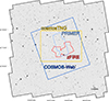 |
Fig. 1. The COSMOS field and the simulated volume by cosmosTNG. The background shows HST-ACS F814W imaging of the field. We show the footprint of cosmosTNG/CLAMATO in the field, along with the zFIRE, COSMOS-Web, and PRIMER survey footprints. |
This paper is structured as follows. In Sect. 2 we describe the initial conditions and simulation setup, the TNG galaxy formation model, and the cosmosTNG suite. In Sect. 3 we present the initial results from cosmosTNG, including the reconstructed large-scale structure and a number of galaxy population statistics and scaling relations in comparison to data. We conclude in Sect. 5 with a summary of the results and a future outlook.
2. Methods
2.1. Initial conditions and simulation setup
In the following we describe our methods for constructing and running constrained simulations. The overall method is summarized in Fig. 2, showing the key steps of reconstruction, initial conditions setup, and running of the hydrodynamical simulation.
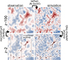 |
Fig. 2. Schematic of the method. We reconstructed the initial z ∼ 100 density field from observations of zCOSMOS galaxies and CLAMATO Lyα forest measurements at z ∼ 2 using the TARDIS pipeline. We then generated constrained initial conditions using our modified version of N-GenIC, and finally ran the full hydrodynamical simulation using the AREPO code. |
The initial conditions are derived from observations of the COSMOS Lyman-alpha Mapping And Tomography Observations (CLAMATO) Survey (Lee et al. 2014a, 2018; Horowitz et al. 2022), supplemented by spectroscopic galaxy samples added in the TARDIS reconstruction method (Horowitz et al. 2019, see Fig. 2 bottom left).
CLAMATO utilizes star-forming galaxies and quasars as background sources to probe the Lyman-alpha (Lyα) forest to determine the large-scale hydrogen distribution at z ∼ 2.05 − 2.55 centered at 10h00m34.21s, +02 ° 17′53.49″ (J2000). This corresponds to an extent of 438 cMpc/h in redshift and 34 cMpc/h in right ascension (RA) and 28 cMpc/h in declination (Dec). The CLAMATO survey was conducted with the LRIS spectrograph on the Keck-I Telescope, yielding around 320 galaxy and quasar background sources in a ∼0.2 deg2 patch of the COSMOS field. The Lyman-alpha forest fluctuation is determined for each sightline by dividing out the estimated source continuum and assumed mean Lyman-alpha transmission (Lee et al. 2012).
While earlier Lyman-alpha forest based reconstruction efforts (Lee et al. 2014a, 2018; Newman et al. 2020) used the Wiener filtering technique (see, e.g., Pichon et al. 2001; Caucci et al. 2008) for reconstruction of the large-scale density field, cosmosTNG uses the more recent TARDIS method (Horowitz et al. 2019, 2021, 2022) allowing the reconstruction of the initial density field from the CLAMATO survey. The Tomographic Absorption Reconstruction and Density Inference Scheme (TARDIS) utilizes maximum likelihood methods to reconstruct the underlying initial density field with a fast nonlinear gravitational model. A forward model computes the mock Lyα forest measurements and galaxy populations by evolving a given initial density field with the fastPM/flowPM code (Feng et al. 2016; Modi et al. 2021) to the target redshift. A similar forward model based reconstruction approach has been studied in Porqueres et al. (2019, 2020) utilizing a Hamiltonian Monte Carlo solver, albeit requiring a strong cosmological prior and larger computational demand.
For the Lyα forest transmission, the Fluctuating Gunn-Peterson Approximation (FGPA) yields the evolved density field. The improved TARDIS-II allows galaxies to be incorporated into the reconstruction, which we do so by including galaxy redshifts taken from zCOSMOS (Lilly et al. 2007), including unpublished zCOSMOS-Deep data (Kashino et al., in prep.). The galaxy overdensity field is modeled using a linear and quadratic bias term in Lagrangian space, effectively following the approach in Modi et al. (2020). The log-likelihood for the Lyα forest and galaxy population consists of a prior term and the sum of the squared differences between the respective observed and model overdensity field in each pixel. The joint log-likelihood is given by the sum of the two individual log-likelihoods1. The prior is chosen to enforce positivity of the power spectra band powers, but without a strong cosmological constraint on the fields. The likelihood is iteratively maximized by running a sequence of forward models using the limited-memory Broyden-Fletcher-Goldfarb-Shanno (LBFGS; Liu & Nocedal 1989) optimization algorithm. A detailed description of the reconstruction method can be found in Horowitz et al. (2021, 2022).
For cosmosTNG, each TARDIS forward step was carried out on a 1283 uniform grid with a spatial resolution of 1.0 cMpc/h. The resulting reconstructed density field centers on the CLAMATO survey footprint in RA and Dec at a given redshift. In order to cover the whole CLAMATO survey volume across the redshift range, five overlapping, equally spaced subvolumes were run. These are centered at 59, 147, 235, 323, and 411 cMpc/h in the redshift direction. For each subvolume, we discarded the first and last 5 cMpc/h. This leaves an overlap of 30 cMpc/h between each subvolume. We linearly interpolated the density field in the overlapping region by averaging the densities weighted by the distance to the respective subvolume border. We truncated the stitched density field at 450 cMpc/h. Overall, the end result is a 128 × 128 × 450 grid centered on the CLAMATO survey footprint in RA and Dec2.
From the TARDIS maximum a posteriori realization of the density field, we extracted a 1283 cube for the initial density field of our cosmological simulation. We selected a subvolume in order to reduce the total computational cost of the project, although initial conditions for the entire 450 cMpc/h volume can be run in the future. The particular subvolume was chosen for two reasons: minimal contamination from overlap, and coverage of the well-studied zFIRE proto-cluster region.
Next, we converted this density field to a high-resolution set of particles for the initialization of the AREPO simulations. Conceptually, this was done by sampling the density field supplemented by random small-scale fluctuations according to the concordance cosmology model, then applying the Zeldovich approximation to obtain the initial particle positions and velocities. Practically, we created a custom version of the MPI-distributed N-GenIC code (Springel et al. 2005). The modified version improves memory efficiency for noncubical simulation volumes and allowed us to fix the large-scale density field and add small-scale fluctuations according to the linear power spectrum.
We started by creating an unperturbed particle distribution, where the target volume is embedded into a larger periodic volume. The periodic volume is cubical with side length L with L = 512 Mpc/h. The cubical volume is sampled with Nbase3 uniformly spaced particles on a Cartesian grid with Ngrid = 128, inside of which we embedded the 34 × 28 × 118 cMpc3/h3 subvolume at our target resolution in the box center. Between the base and target resolution, all intermediate mass resolution levels differ by a factor of eight in mass. We padded the target volume with at least two boundary particles per intermediate resolution level between target and base resolution.
We then upsample the previously reconstructed density field using linear interpolation to a uniform grid with Ngrid = 2 ⋅ Nbase elements in each dimension covering the periodic volume L3. We compute the Fourier transform of this field to filter out any unconstrained small-scale power above a cutoff frequency kcutoff = 1 h/cMpc. Particle displacements and velocities are then derived using the Zeldovich approximation (Zel’dovich 1970) at the unperturbed particle positions. The displacements and velocity shifts are applied to all particles within the 1283 cMpc3/h3 input data cube. As such, we also capture large-scale modes outside of the CLAMATO field as reconstructed by TARDIS. Particles outside of the loaded density field do not receive any displacement or velocity.
Next, we added small-scale density fluctuations above the cutoff frequency. A uniform complex grid representing the Fourier transform of this density field was initialized to zero. This grid has an extent of Dx, y, z = (64, 64, 256) cMpc/h covering the target volume with a grid size of Nx, y, z = 21 + ceil(log2(Dx, y, z/Δ)). For all modes with k > kcutoff, we drew random numbers from a Gaussian distribution under Hermitian constraints to generate the Fourier transform of a real Gaussian random field (Sirko 2005). Properly normalized, we multiplied this field with the square root of the linear power spectrum to obtain a realization for the small-scale fluctuations. The linear matter transfer function was computed using the CAMB code (Lewis et al. 2000) assuming Planck15 cosmological parameters (see Sect. 2.4). Displacements and velocities were added for these particles at the target resolution. To match the mass target resolution, we used a sampling factor 0.5 < f < 1 (Δsampling = Δ/f) and a Cloud-in-Cell interpolator at the sampled positions.
The resulting initial condition at z = 127 contains total matter particles. Upon initialization of the simulation, each original particle was split into a dark matter particle and gas cell and displaced from one another by half the mean spacing, while conserving the center of mass of the pair.
Figure 3 shows the power spectrum within the cosmosTNG simulation volume. The blue line shows the power spectrum of the TARDIS reconstruction, while the CAMB-based linear expectation is shown in orange. The TARDIS reconstruction power drops off around the chosen cutoff frequency k ∼ 1 h/cMpc, reflecting the limited small-scale constraints as well as the reconstruction grid resolution. The chosen cutoff frequency coincides well with the constrained power dropping below the linear expectation. The colored shaded areas reflect the regimes within which we take the TARDIS reconstruction and random realization respectively.
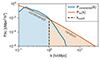 |
Fig. 3. Power spectrum of the simulation volume at its initial condition (z ∼ 127). Blue shows the power of the constrained field (large scales) in the 34 × 28 × 450 cMpc3/h3 volume. Orange shows the theoretically expected linear power. The shaded region shows the composite realization for the cosmosTNG simulations: modes are from the constrained field up to kcutoff = 1 h/cMpc above which we randomly draw modes according to linear theory. |
Using the previous output, we performed the evolution step using the AREPO code. In the following, we show and discuss a dark matter-only run of the full CLAMATO volume, before introducing the TNG model (Sect. 2.2) for the hydrodynamical runs. The dark matter-only evolution of the full CLAMATO volume using AREPO is shown in Fig. 4, where we visualize the evolved initial conditions at redshift z ∼ 2.3. In the top panel, we show eight consecutive 4 cMpc/h thick projections stepping through the right ascension direction. We additionally show observed galaxies from the spectroscopic DEIMOS (Hasinger et al. 2018), zCOSMOS (Lilly et al. 2007) and zFIRE (Nanayakkara et al. 2016) surveys. The cosmosTNG simulation subvolume is shown as the rectangular region spanning from z ∼ 2.06 to z ∼ 2.19, containing the prominent zFIRE protocluster (Spitler et al. 2012; Nanayakkara et al. 2016). In the bottom panel, we show five Δz ∼ 0.1 projections of the dark matter density field with redshift along the line-of-sight direction. Orange rectangles show the nontrivial footprint of the zFIRE survey, the largest source of spectroscopic galaxies in this region. We also mark photometric detections from the COSMOS2020 catalog (Weaver et al. 2022) as hexagons.
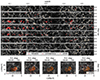 |
Fig. 4. Visualization of the full constrained region evolved to z ∼ 2 from which cosmosTNG is drawn. Top: Eight consecutive projections of 4 cMpc/h thick projection of the dark matter density field showing the redshift (resp. declination) on the x-axis (resp. y-axis). Bottom: Five projections of the same dark matter density field as a function of right ascension and declination at increasing redshifts. The colored symbols show observed galaxies from spectroscopic redshift surveys. In the orange rectangles we show the zFIRE survey footprint. In the lower panel we additionally show photometric detections from the COSMOS2020 catalog as hexagons. |
2.2. The TNG galaxy formation model
The TNG galaxy formation model is implemented within the AREPO code (Springel 2010), which solves the coupled equations for self-gravity and ideal, continuum magnetohydrodynamics (Pakmor et al. 2011). The physical domain is discretized with a moving Voronoi tessellation, which allows for a quasi-Lagrangian description of the gas dynamics. The TNG model has been used in several large-volume projects across different regimes and redshifts: the TNG100 and TNG300 simulations of IllustrisTNG (Springel et al. 2018; Nelson et al. 2018; Pillepich et al. 2018b; Naiman et al. 2018; Marinacci et al. 2018), the TNG50 volume (Pillepich et al. 2019; Nelson et al. 2019a), THESAN (Kannan et al. 2022; Garaldi et al. 2022; Smith et al. 2022) MillenniumTNG (Pakmor et al. 2023), and TNG-Cluster (Nelson et al. 2024). We briefly summarize the TNG model physics here (see Weinberger et al. 2017; Pillepich et al. 2018a).
The TNG model includes the processes essential for galaxy formation: primordial and metal-line cooling; heating and ionization from an ultraviolet background (UVB; Faucher-Giguère et al. (2009), FG11 version); star formation above a density threshold (Springel & Hernquist 2003); stellar feedback driven galactic winds; stellar population evolution and chemical enrichment from supernovae Ia, II, and AGB stars (Pillepich et al. 2018a); and the seeding, merging, accretion growth, and feedback of supermassive black holes (SMBHs; Weinberger et al. 2017).
Stellar feedback combines (i) a treatment of small-scale pressure arising from unresolved supernovae generating the hot-phase of the ISM, together with (ii) a decoupled kinetic wind method that produces galactic-scale outflows (Springel & Hernquist 2003). At injection, the wind velocity is set to be proportional to the local dark matter velocity dispersion at a minimum of 350 km/s and a mass loading of  , where τwind = 0.1 is the thermal energy fraction and ewind is a metallicity dependent modulation of the canonical energy available per SNII (see Pillepich et al. 2018a, for details). The resulting feedback-driven outflows collimate along the minor axes of galaxies, with velocities and mass loadings that decrease with distance (Nelson et al. 2019a).
Supermassive black hole feedback follows the description in Weinberger et al. (2017). The two-state model switches from a kinetic to a thermal mode feedback for high accretion rates relative to the Eddington limit. In addition, radiative feedback is implemented in the form of photoheating and -ionization from a local AGN ionization field impacting up to 3 times the virial radius of the host halo (Vogelsberger et al. 2014). The AGN luminosity is proportional to the accretion rate above a target accretion threshold, modified by an obscuration factor (Hopkins et al. 2007). The radiation field is added under the assumption of optically thin gas, scaling as 1/r2 from its source, and is subject to the same self-shielding description as for the UV background.
2.3. The cosmosTNG suite
The numerical resolution of the cosmosTNG simulations are given in Table 1. The primary runs have a dark matter mass resolution of mDM = 7.5 × 10⁶ M⊙ and a gas mass resolution of mgas ∼ 1.4 × 10⁶ M⊙ in the high-resolution 34 × 28 × 118 cMpc3/h3 subvolume. To study numerical convergence, we also run lower resolution versions of every volume, labeled ‘–2’ (8 times lower mass resolution) and ‘–3’ (64 times lower mass resolution). These resolution levels are equal to those of TNG100, and cosmosTNG-1 has the same resolution as TNG100-1. For each run we save 34 snapshots down to redshift z = 2.
Comparison of cosmosTNG resolution levels.
We run eight variations of cosmosTNG. Each has different density fluctuations for the unconstrained, small-scale modes. The variations are denoted by a letter from A to H, and each letter represents a different random seed, used to initialize and draw a pseudorandom number sequence used to set the amplitudes and phases above the cutoff frequency kcutoff = 1 h/cMpc (see Fig. 3). These variations allow us to study the impact of small-scale variations on the galaxy properties while keeping the large-scale structure fixed. A summary of properties for the variations is shown in Table 2.
cosmosTNG small-scale variation runs.
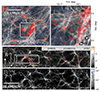 |
Fig. 5. Visual overview of the cosmosTNG-A simulation at z = 2. Top panel: Two 30 cMpc/h projections along the redshift direction with the right ascension (declination) on the x-axis (y-axis). On the left, we show the CLAMATO footprint, and on the right a zoomed-in view of a highly overdense region studied by the zFIRE survey. Both projections show a two-dimensional color map, where blue (red) indicates cold (hot) gas, and white (black) indicates high (low) density. The red symbols in the upper panels show observed galaxies from various spectroscopic surveys. Bottom panels: Dark matter and stellar density projections for a 10 cMpc/h thick slice through the simulation volume with the redshift (declination) on the x-axis (y-axis). Visually, we find that observed galaxies spatially correlate with the simulated density field down to the reconstruction scale of 1 cMpc/h. This correlation is particularly striking in the redshift direction within the zFIRE region, reproducing a characteristic arc shape of the galaxy distribution. |
2.4. Conventions
We use ‘p’ and ‘c’ to explicitly note comoving or physical coordinates across the paper. In the analysis, unless stated otherwise, stellar masses and star formation rates are computed in an aperture with 2 arcsecond diameter. Halo masses are taken as the total mass of a Friends-of-Friends group enclosed in a sphere whose mean density is 200 times the critical density of the universe at the respective redshift. For calculating all statistics, we ignore the outer 2 cMpc/h of the target volume to mitigate numerical effects in the proximity of low-resolution particles.
For TARDIS and AREPO, we assume a concordance flat ΛCDM cosmology with ΩΛ, 0 = 0.6911, Ωm, 0 = 0.3089, Ωb, 0 = 0.0486, σ8 = 0.8159, ns = 0.9667, and h = 0.6774, consistent with Planck Collaboration I (2016). For mapping from comoving Cartesian coordinates to celestial coordinates and redshift we use a fixed relation χ = 3874.867 cMpc/h and dχ/dz = 871.627 cMpc/h at ⟨z⟩ = 2.30 for simplicity3.
3. Results
In Fig. 5 we show an overview plot of the simulated cosmosTNG volume that displays several different physical properties. The two panels at the top show the density-temperature map of a zoomed-in region centered on the zFIRE protocluster region at z = 2 in the right-ascension-declination plane. Blue (red) colors indicate cold (hot) gas, while white (black) indicates high (low) density. We see a web of filamentary structures at intermediate temperatures, with hot gas present and abundant at its nodes. In the two lower panels, we show the average dark matter and stellar mass density in the redshift-declination plane.
For qualitative comparison, red markers indicate observed spectroscopic galaxies (top three panels). We generally see good visual agreement between simulated overdensities and observed galaxies on ∼ Mpc scales, near the constrained modes of the initial conditions. Due to irregular survey footprints, the correctness of observed galaxy overdensities is hard to assess in RA–Dec projections. For the redshift-declination projection of the dark matter density however, we see good agreement between observed and simulated structures as visually confirmed by the arc-like structure of the protocluster region.
In Fig. 6 we show projections for the redshift-Dec plane for the neutral hydrogen column density, gas temperature, and gas metallicity. In the top panel, we also show simulated galaxies and black holes with masses above 1010 M⊙ and 108 M⊙, respectively. The cosmic web is clearly visible in the various panels, and filamentary structures are particularly pronounced in the neutral hydrogen density maps, covering a large dynamical range: from < 1014 cm−2 in voids, to filaments often in excess of 1017 cm−2 and reaching > 1020 cm−2 in large overdensities. The temperature map, as well as galaxy and black hole positions also trace the large-scale structure, albeit more biased toward overdense nodes of the cosmic web, often exceeding 106.5 K in the proximity of massive galaxies. Heated regions near cosmic web nodes are accompanied by metal-enriched gas (> 10−1 Z⊙) up to scales of multiple cMpc, indicating AGN-driven outflows out to these scales and beyond.
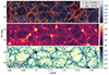 |
Fig. 6. Projections of the neutral hydrogen column density (top), temperature (middle), and metallicity (bottom) along the RA direction through the cosmosTNG-A simulation at z = 2 for a 10 cMpc/h depth with the redshift (declination) on the x-axis (y-axis). In the top panel, we also mark simulated galaxies and black holes with masses above 1010 M⊙ and 108 M⊙, respectively. Thin filaments of neutral hydrogen span the volume and at its nodes, massive galaxies reside whose AGN heat and metal-enrich their surroundings. The white box in the top panel indicates the zFIRE cluster zoomed-in region shown in Fig. 5. |
3.1. Stellar mass function and stellar-to-halo-mass relation
We begin our quantitative analysis of cosmosTNG with integral properties of the galaxy population. In the top panel of Fig. 7, we show the galaxy stellar mass function (SMF) at redshifts z ∼ 2, 4, 6. We measure the stellar mass within a 2.0 arcsecond diameter aperture, and including all subhalo stars. The bands show the range of outcomes of the eight different variation runs, and the red lines show the TNG100 result. Gray symbols show observational data (Ilbert et al. 2013; Muzzin et al. 2013; Davidzon et al. 2017; Leja et al. 2020; Weaver et al. 2023) for z ∼ 2.0 − 2.5.
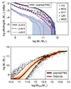 |
Fig. 7. Top: Galaxy stellar mass function from cosmosTNG at redshifts z = 2, 4, 6. The semi-transparent bands span the outcomes of different variation runs with the embedded line showing the mean. In red we show the TNG100 simulation outcomes. We compare these simulations to several observational datasets (Ilbert et al. 2013; Muzzin et al. 2013; Davidzon et al. 2017; Leja et al. 2020; Weaver et al. 2023) at face value. These observations span z ∼ 2.0 − 2.5 and are shown with gray markers. In comparison to TNG100, cosmosTNG produces more high-mass galaxies above 1011 M⊙ by up to 0.5 dex. This reflects the overabundance of massive dark matter halos in this region (see text). Bottom: Relation of stellar mass to halo mass for stellar masses within the previous aperture of all central galaxies and the mass of their hosting halo at z = 2. The orange contours indicate the distribution of stellar masses at fixed halo mass across all cosmosTNG variation runs, while the individual points show galaxy outliers. The solid black (red) line shows the median stellar mass for cosmosTNG (TNG100). |
When comparing to observations, here and through the results section, we use various recent observational datasets to give a sense of the variation due to different observational methods and target selection functions, allowing better face-value comparisons against cosmosTNG and TNG100.
The TNG100-1 result is within 0.5 dex of the data at these redshifts, always in the direction of having too many galaxies at a given stellar mass. We stress that differences in methodology and aperture corrections make quantitative comparisons to data difficult (see also Pillepich et al. 2018b, for previous comparisons of the TNG100 and TNG300 SMFs with data). While generally on the upper end, cosmosTNG and the TNG model are broadly consistent with observational results from Leja et al. (2020), who employ a continuity model accounting for the redshift evolution of the mass function within the fitting procedure. The level of disagreement between the observational inferences suggests that systematic uncertainties are similar to the level of (dis)agreement seen between the observations and simulations.
Of primary interest, cosmosTNG is consistent with TNG100 only at stellar masses below 1011 M⊙. At higher masses, cosmosTNG exceeds the number of galaxies compared to TNG100, as well as general (i.e., non-COSMOS) field observations. At this high-mass end, the galaxy count in cosmosTNG exceeds that of TNG100 due to a shallower slope of the SMF. This discrepancy is largest at high redshifts and decreases toward z ∼ 2. This behavior is consistent across all variation runs. Given the identical galaxy formation model and resolution, the constrained initial conditions produce this difference. Specifically, a higher abundance of high-mass galaxies is driven by an excess of large-scale density fluctuations (see Fig. 3) at k < 1 cMpc/h. In Fig. A.1 we show the halo mass function at z = 2, and its evolution from the initial conditions. An excess abundance of massive dark matter halos with respect to a random region of the universe directly leads to the z ∼ 2 excess in the high-mass end of the SMF.
In the bottom panel of Fig. 7, we show the stellar mass to halo mass relation M⋆ − Mhalo at z = 2 for cosmosTNG and TNG100. The relation follows a step power-law scaling up to approximately Mhalo = 1012 M⊙ after which the relation significantly flattens in line with the SMF drop off. While next to identical at lower masses, there is a mild 0.1–0.2 dex higher median relation for cosmosTNG compared to TNG100 above Mhalo = 1012 M⊙, contributing to the massive galaxy overabundance in the SMF.
3.2. Star formation rate history
In Fig. 8 we show the cosmic star formation rate density (SFRD) as a function of redshift. The SFRD is calculated as the sum of instantaneous star formation in each gas cell divided by the simulated volume at target resolution. The black dashed line shows the mean of all 8 variation runs and individual colored lines show the evolution for individual runs. The red line shows the same line for the TNG100 simulation (see Shen et al. (2022) for dust modeling and obscured star formation effects in the SFRD, and Pillepich et al. (2018a) for the impact of physical model choices on the SFRD, in the context of the TNG simulations).
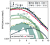 |
Fig. 8. Cosmic star formation rate density (SFRD) in cosmosTNG between z = 2 − 10. The colored lines show the individual realizations, and the black line shows the average. In red we show the TNG100 simulation for comparison. Semi-transparent bands show the range contributions of different stellar mass ranges to the overall SFRD budget across different variation runs. The gray points indicate observational data from various surveys (abbrv. R09, M11, C12, M13, G13, B15 for Reddy & Steidel 2009; Magnelli et al. 2011; Cucciati et al. 2012; Magnelli et al. 2013; Gruppioni et al. 2013; Bouwens et al. 2015), with some data from Madau & Dickinson (2014), Bouwens et al. (2015). We compare this data to cosmosTNG at face value (i.e., without replicating the procedure for the observational inferences). The SFRD of cosmosTNG is overall higher, and peaks at earlier redshift, than the field result of TNG100, suggesting that z ∼ 2.1 galaxies within this region of COSMOS have undergone a particularly active assembly history. |
The eight variation runs deviate by less than 20–30% from one another, with relative differences being the largest around z ∼ 7. Strikingly, the cosmosTNG mean and all variation runs are consistently higher than TNG100 at all redshifts. The relative difference between cosmosTNG and TNG100 peaks around z ∼ 4 with cosmosTNG having nearly twice as much star formation taking place. Furthermore, cosmosTNG reaches its maximum SFRD earlier at z ∼ 3.5 compared to z ∼ 3 for TNG100.
Gray markers show observationally inferred SFRD values (Madau & Dickinson 2014, and others, see the figure caption for details). The SFRD inferred, particularly at cosmic noon between z ∼ 2 − 3, shows significant variation across observational studies. At face value, these are consistent with cosmosTNG down to its maximum at redshift z ∼ 3.5. In contrast to the TNG model, many observationally inferred SFRDs keep rising toward z ∼ 2, leading to discrepancy of up to roughly a factor of two depending on the dataset at this redshift (however, see Enia et al. 2022, for systematics and further discussion, including a relatively flat inferred SFRD from z ∼ 2 to z ∼ 3.5).
In Fig. 8 we also show how different halo masses contribute to the global SFRD (following Genel et al. 2014, with Illustris). We sum all star formation associated with subhalos in a given stellar mass range, and plot the range of outcomes between different variation runs as shaded bands. Here, stellar masses are computed summing over all stars belonging to a subhalo.
We find that galaxies with stellar masses from 1010 to 1011 M⊙ dominate between 2 < z < 7, even though contributions for galaxies from 109 to 1010 M⊙ have nearly equal weight. Interestingly, the overall turnover at z ∼ 3.5 does not occur for these mass bins, but is instead driven by galaxies with lower as well as higher mass. Star formation in halos between 108 to 109 M⊙ and 1010 to 1011 M⊙ equally contribute roughly 10% each to the overall budget at z ∼ 3.5, where they both peak. However, lower mass halos already contribute more substantially at higher redshifts. The SFRD of low-mass halos < 108 M⊙ peaks at z ∼ 5, and declines toward higher as well as lower redshift.
3.3. Galaxy size-mass relation
In Fig. 9 we show the size-mass relation for central galaxies in cosmosTNG at z = 2. Orange contours show the distribution of galaxy sizes at fixed galaxy mass. Dots represent individual galaxies that are outliers with respect to the main population. Here we measure galaxy size as twice the stellar half mass radius, and galaxy mass as the stellar mass contained within a sphere of this size, in order to be self-consistent. The solid black line shows the median relation, while colored dashed lines show the z = 2 median for individual variation runs.
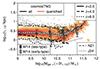 |
Fig. 9. Size–mass relation in cosmosTNG at z = 2, combining all central galaxies regardless of type. The orange contours indicate the distribution of sizes at fixed stellar mass across all cosmosTNG variation runs, while the individual black points show outliers. The black line shows the median size at fixed stellar mass. The dashed (dotted) line shows the median at redshift z = 4 (z = 6), while the colored dashed lines show the individual variation runs. Finally, the red dots and the red line show quenched galaxies only (see text). We define galaxy size as twice the stellar half-mass radius, and here measure stellar masses summing all stellar populations within this radius. The observational data span z = 2.0 to z = 2.5 (van der Wel et al. 2014), where open symbols show early-type galaxies and filled symbols show late-type galaxies. Additionally, we show the linear scaling relations for quenched galaxies derived from observations Nedkova et al. (2021) and Ji et al. (2024) with gray lines. The observational data is compared as-is, without any further observational mock post-processing of cosmosTNG. |
For low-mass galaxies, the distribution and median of galaxy sizes is roughly constant with a median size of ∼2.5 pkpc (resolution convergence at the low-mass end and smaller galaxy sizes in TNG50 are discussed in Pillepich et al. 2019). At a stellar mass of 1010.8 M⊙ sizes start to increase rapidly, toward a power-law slope of ∼2/3. The turning point at 10.8 M⊙ coincides well with the turnover for the sSFR(M⋆) relation in Fig. 10.
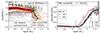 |
Fig. 10. Star formation activity of galaxies. Left: Specific star formation rate (sSFR) as a function of stellar mass for central galaxies in cosmosTNG at z = 2. The annotations and markers are as in Fig. 7, bottom panel. Measurements are within 2 arcsecond diameter apertures and with a 100 Myr averaged SFR. The gray markers show the inferred sSFR from observations in Whitaker et al. (2014). The dashed gray line shows the sSFR ridge from observational modeling in Leja et al. (2022). Right: Quenched fraction as a function of stellar mass in cosmosTNG and TNG100 at z = 2. The error bars show the observations from Sherman et al. (2020), Park et al. (2024) around cosmic noon. The observations are compared as-is (i.e., without reproducing the methodology used in the simulation). Quenched galaxies are defined as having a star formation rate at least 1 dex below the main sequence (see text). The colored lines show the individual realizations, and the dark solid line shows the average for all galaxies. The dashed (dotted) line shows the average for central (satellite) galaxies. A sizable population of quenched (central) galaxies with M⋆ > 1010.5 M⊙ is already present by z = 2. We see a lower quenching for cosmosTNG galaxies compared to TNG100. |
Red points and the red line show quenched galaxies and their median relation only, visible for M⋆ > 1010.5 M⊙. We see that quenched galaxies in cosmosTNG, as in observations, are smaller than the overall sample by 0.2–0.4 dex, with the largest difference at M⊙ ∼ 1010.5 M⊙. The difference vanishes toward higher masses as quenched galaxies start to dominate the overall sample (see Genel et al. 2018, for a discussion on the broad agreement of TNG galaxy sizes with data, as a function of redshift as well as split by star formation activity, representing an important model validation outside of the scope of calibrated observables).
The dashed (dotted) black lines show the median galaxy size at higher redshift, z ∼ 4 (z ∼ 6). At earlier times, galaxies at fixed mass are smaller, and there is a pronounced trend of smaller size with increasing mass (see also Costantin et al. 2023; Karmakar et al. 2023; Du et al. 2024).
We furthermore show observational data from van der Wel et al. (2014) for various stellar mass bins, for the late-type galaxy population (filled symbols), and early-type galaxies. Gray lines show the linear scaling relations for quenched galaxies as inferred from observations at z = 1.5 − 2.0 and z = 2.0 − 2.5 in Nedkova et al. (2021) and Ji et al. (2024) respectively. While we generally find good agreement with van der Wel et al. (2014), the largest discrepancy exists at stellar masses close to the turning point of 10.8 M⊙. The observations indicate a more constant slope of size growth with mass across this range. Finally, we see sizes at the high-mass end in good agreement with Nedkova et al. (2021), while the near-infrared observations from Ji et al. (2024) generally point toward substantially smaller galaxy sizes and a shallower trend with mass.
3.4. Specific star formation rates, quenching, and gas budget
In Fig. 10 we show the star formation activity of galaxies in terms of the specific star formation rate (sSFR; left panel) and the quenched fraction (right panel) as a function of stellar mass in cosmosTNG at z ∼ 2. The sSFR and stellar masses are measured in a 2 arcsecond diameter aperture, and the sSFR is averaged over the last 100 Myr prior to z = 2.
We determine the quenched fraction by counting those galaxies with a star formation rate that is 1 dex below the main sequence (SFMS). The simulated main sequence is determined with an iterative scheme following Donnari et al. (2021), where we compute the median star formation rate in stellar mass bins of 0.2 dex, excluding all galaxies 1 dex below this median value as quenched. This procedure is then repeated until convergence. We then take all nonquenched galaxies in the stellar mass range from 109 to 1010.2 M⊙, fit a linear relation in the log M⋆ − logSFR-plane, and label all galaxies 1 dex below this line as quenched. For reference, the blue dashed line shows the SFMS, and the red dashed line shows the threshold for quenched galaxies.
For the left panel of 10, we include central galaxies from all 8 variation runs. Red contours show the sSFR distribution at fixed stellar mass, while black points show individual galaxies where the sampling is sparse. We indicate the median sSFR relation for cosmosTNG (TNG100) with a solid black (red) line. The median lines for cosmosTNG and TNG100 closely align and follow the SFR ridge seen in the contours.
We overplot the SFR ridge from observational modeling in Leja et al. (2022) with the dashed gray line. Overall, it is ∼0.2 dex higher than the sSFR ridge in cosmosTNG. Inferred observational values from Whitaker et al. (2014) are higher by around 0.5 dex. Similar to the parametric drop of the SFR ridge slope at 1010.6 M⊙ in Leja et al. (2022), we find a decrease in cosmosTNG around 1010.8 M⊙, albeit with a substantially steeper slope. The sSFR distribution becomes significantly broader for these high-mass galaxies (see also Ilbert et al. 2015).
In the right panel, we show the quenched fraction of all (central, satellite) galaxies in cosmosTNG at z ∼ 2 as gray solid (dash-dotted, dotted) line. The thin dashed lines show the quenched fraction for the individual variation runs, and the solid red line the quenched fraction in TNG100 (see Donnari et al. 2019; Gupta et al. 2021). We show observational measurements for the quenched fraction (Sherman et al. 2020; Park et al. 2024). Sherman et al. (2020) compute the quenched fraction for a sample of roughly ∼30 000 massive galaxies, combining photometric data from DECam with other bands to perform spectral energy distribution fitting in large area surveys covering a total of 17.5 deg2. Park et al. (2024) shows a recent JWST result of quenched fractions using deep NIRSpec spectra from the Blue Jay survey, overlapping in parts with cosmosTNG. Both observational datasets use the same quenched definition (1 dex below the SFMS) as here. For the observed redshift range (2 < z < 2.5 for Sherman et al. 2020 and 1.7 < z < 3.5 for Park et al. 2024), there is a 20 percent point higher quenched fraction at z ∼ 1010.7 M⊙ in Park et al. (2024). Alternatively, the difference can be interpreted as a ∼0.25 dex shift toward lower stellar mass bins at fixed quenched fraction. This highlights potential effects from different target selections and available data for SED fitting, while environmental effects might also be at play. 4 of the 16 quenched galaxies in Park et al. (2024) fall into the zFIRE protocluster covered by cosmosTNG.
cosmosTNG is in good agreement with Sherman et al. (2020), while results from Park et al. (2024) suggest an onset of quenching at lower masses, more similar to that of the TNG100 simulation. We note that if the difference between Sherman et al. (2020) and Park et al. (2024) is a true environmental effect, it goes in the opposite direction as seen in our two simulations.
While the quenched fraction curves for both cosmosTNG and TNG100 follow a very similar shape, there is a significant offset between M⋆ ≃ 1010.5 M⊙ and M⋆ ≃ 1011.5 M⊙. On one hand, such galaxies in cosmosTNG reach the quenched fraction found in TNG100 at a 0.4 dex higher stellar mass. Alternatively, galaxies of a given stellar mass have a ∼20 percent lower quenched fraction. We investigate this compelling difference in quenched fractions between cosmosTNG and TNG100 in the discussion.
In Fig. 11 we show the gas fraction relative to the central galaxy host halo mass (top) and galaxy stellar mass (bottom). The stellar and gas masses are computed within twice the stellar half-mass radius of the central galaxies. In the upper panel, we see the median gas fraction Mgas/Mhalo staying roughly constant between 1010 to 1012 M⊙ at ∼1%, while there is a modest enhancement around 1011.5 M⊙ and increased scatter toward lower stellar masses. Above 1012 M⊙ the median quickly drops to ≲0.1% at 1013 M⊙ with the scattering widening again. The drop at 1012 M⊙ coincides with the flattened M⋆–Mhalo relation (see Fig. 7), while latter relation shows significantly less scatter beyond this mass threshold. The lower panel shows the gas fraction in terms of the stellar mass, showing a monotonously decreasing Mgas/M⋆, dropping below unity around 1010 M⊙. At 1010.7 M⊙, we see a substantial drop similar to sSFR(M⋆) in Fig. 10.
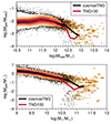 |
Fig. 11. Gas fraction for all central galaxies relative to their hosting halo mass (top) and their stellar mass (bottom) in cosmosTNG at z = 2. The annotations and markers are as in Fig. 7, bottom panel. The gas and stellar mass are calculated within twice the stellar half-mass radius. We see an increased drop and scatter for gas fractions above Mhalo ≳ 1012 M⊙ and M⋆ > 1010.5 M⊙, in line with changes in the M⋆(Mhalo) and sSFR(M⋆) relations. Above these mass thresholds, cosmosTNG galaxies show a higher gas fraction on average. |
3.5. Galaxy number densities
In Fig. 12 we show the number density of galaxies as a function of redshift. In the left (right) panel, we show the number density for all (quenched) galaxies. Blue, orange, and green lines give the result for three different lower galaxy stellar mass thresholds of 1010.0, 1010.5, and 1011.0 M⊙. Bands show the variation in the number density across different variation runs. For comparison, dashed lines show the number densities of galaxies from TNG100.
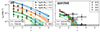 |
Fig. 12. Number density of all (i.e., central and satellite) galaxies as a function of redshifts above a given stellar mass threshold in cosmosTNG-1. The shaded regions show the variation in number density across all random variations. The solid lines show the respective mean. Left: All galaxies (observational data from Weaver et al. 2023). Right: Quenched galaxies (observational data for quenched galaxy densities from Merlin et al. 2019; Carnall et al. 2020; Gould et al. 2023; Carnall et al. 2023). Observations are compared at face value without observational mock post processing of cosmosTNG. The hatched region at the bottom shows the number density 1/Vsim (i.e., one galaxy within the cosmosTNG simulation volume Vsim). |
In the left panel, at redshift z = 2, we find the number density of massive galaxies ≥1011 M⊙ in cosmosTNG to exceed those in TNG100 by a factor of 2–3, consistent with the shape of the SMF in Fig. 7. This difference disappears at lower mass thresholds. In contrast, it is generally strong at all mass thresholds for higher redshifts. For quenched galaxies (right panel), differences between cosmosTNG and TNG100 are similarly pronounced for M⋆ ≥ 1011 M⊙ for z = 2, and at all masses for z ≥ 3.
The existence and abundance of massive galaxies at high redshift, particularly massive quiescent galaxies, has recently been emphasized as a possible source of tension between observations and models within COSMOS at z ≳ 3 (Forrest et al. 2024a). We therefore show several observational constraints with markers and their associated error bars. For the number density of all galaxies, we integrate the parameterized double Schechter fit from Weaver et al. (2023), and show a conservative upper limit derived from the parameter errors of the Schechter fit. For quenched galaxies, we directly take densities and their uncertainties inferred from various observations (Merlin et al. 2019; Carnall et al. 2020, 2023; Gould et al. 2023). The JWST NIRCam observations presented in Carnall et al. (2023) within the Extended Growth Strip (EGS) show a significant higher estimate than previous observational studies for the number counts of quenched galaxies at 3 < z < 4 and particularly 4 < z < 5. While Carnall et al. (2023) highlight that the high counts arise from better constraints enabled by NIRCam data, further spectroscopic follow-ups might be needed (also see, e.g., Forrest et al. 2024b).
We find the observationally inferred number density of galaxies to be broadly consistent at z = 2 for massive galaxies in TNG model simulations. At lower stellar mass thresholds and higher redshifts, observations are systematically lower compared to cosmosTNG and TNG100. That is, the simulations have more than a sufficient number of massive galaxies at early times, possibly even too many. For example, the number density of galaxies 1010.5 M⊙ from van der Wel et al. (2014) at z ∼ 4.5 is a factor of ∼2 (∼8) lower than TNG100 (cosmosTNG).
At the same time, the qualitative trend is the opposite for the quenched galaxy population. At z ∼ 2 − 3 the simulations and observational inferences are broadly consistent. In contrast, cosmosTNG and TNG100 yield systematically lower number densities than observed for z ≥ 3.5. However, at z > 4 in particular, the volumes of TNG100 and cosmosTNG are too small to expect such systems (horizontal dashed black line). Number densities derived from narrow redshift ranges in fields as small as COSMOS clearly suffer from cosmic variance at the high-mass end. However, the large number density of Carnall et al. (2023) remains in tension with the TNG model and our definitions: these results echo a debate that has become very urgent and popular in the last years (e.g., Valentino et al. 2023). However, we have not here made any detailed mocking of the tracers, definitions, or methods used to determine quiescence in data, making this a face-value comparison.
3.6. Galaxy and black hole co-evolution
In Fig. 13 we study the co-evolution of galaxies with their supermassive black holes. The top panel shows the M⋆–MBH relation for galaxies and their black holes at z = 2 in cosmosTNG. Contours and black points show the distribution of black hole masses at fixed galaxy stellar mass, while the black dashed line shows the median relation. Stellar masses are summed within a 2.0 arcsec diameter aperture. We compare against two observational samples: the gray line shows the median relation with its 1 − σ band from Tanaka et al. (2025), while the gray markers with error bars show individual observed high-z galaxies at z > 4 with JWST/NIRSpec from Harikane et al. (2023).
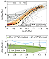 |
Fig. 13. Relation between supermassive black hole mass and galaxy stellar mass, and its evolution with time. Top: MBH–M* relation at z = 2 in cosmosTNG. The gray line shows the linear relation and the 1 − σ scatter from Tanaka et al. (2025). The annotations and markers are as in Fig. 7, bottom panel. Bottom: Evolution of the offset from the local MBH–M* relation as described in Tanaka et al. (2025) based on Häring & Rix (2004), Bennert et al. (2011) for the local relation. The points with error bars show the high-redshift observations from Harikane et al. (2023) and Tanaka et al. (2025). The gray triangles show the observations from Sun et al. (2024). All observations are compared as-is (i.e., without corrections for the respective observational methodology used when compared to cosmosTNG). The green line shows the median relation in cosmosTNG for host galaxies with M⋆ > 1011 M⊙. The shaded regions show the central 68%, 95%, and all percentiles respectively. The blue dashed line shows host galaxies with M⋆ > 108.5 M⊙. The observed galaxies with high black holes masses are rare but possible in cosmosTNG across z = 2 − 5. |
Recent observations of high redshift SMBHs have suggested they may be ‘overmassive’ with respect to the z = 0 expectation, given their host masses, constraining possibly seeding scenarios (Maiolino et al. 2024; Bogdán et al. 2024). The lower panel of Fig. 13 therefore quantifies the redshift evolution of the deviation of black hole masses from the local M⋆–MBH relation, expressed by the relative offset Δlog(MBH/M⊙):

We use the local relation based on Häring & Rix (2004) and Bennert et al. (2011) with αlocal = 0.97 and βlocal = −2.48 (Tanaka et al. 2025). We compute the deviation Δlog(MBH/M⊙) for all galaxies with M⋆ > 1011.0 M⊙ and show the median relation as the green line. Shaded regions show the range containing the central 68%, 95%, and all galaxies. We find a positive median deviation, offset from the local relation by ∼0.5 dex between z = 2.0 − 3.5, suggesting that massive galaxies at this epoch indeed host overmassive SMBHs. The median of the offset decreases toward higher redshift, and drops below the local relation at z ∼ 4.5. Observations from Tanaka et al. (2025) at z ∼ 2 are broadly consistent with cosmosTNG. The observational sample from Sun et al. (2024) indicates no significant redshift evolution between z ∼ 2 − 4, compatible with the simulation. In contrast, observations at z > 4 from Harikane et al. (2023) indicate much larger, positive deviations from the distribution in cosmosTNG. However, we find that this difference is driven largely by the (lower) stellar masses of observed host galaxies. The blue line shows the maximum Δlog(MBH/M⊙) offset in cosmosTNG when we adopt a lower galaxy mass cutoff of M⋆ > 108.5 M⊙. In this case, deviations of up to 2 dex from the local median relation exist across the entire redshift range. We conclude that systems with mass ratios similar to the Harikane et al. (2023) sample can be found in cosmosTNG, although they may represent outliers to the general population. This suggests the need for a more careful analysis of selection functions, in order to assess whether observed black hole masses in galaxies at z ∼ 4 are compatible with cosmosTNG, and TNG model simulations in general.
3.7. Run variations within protocluster regions
In Fig. 14 we focus in on one of the unique regions in the cosmosTNG volume, and its properties across our eight variation runs: the zFIRE protocluster (z = 2.11). In particular, we show projections of gas density and temperature in the RA–Dec plane. The inset shows a zoomed-in image of the most massive halo in the field.
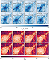 |
Fig. 14. Gas density and temperature projection at z = 2 for the same comoving protocluster region across all eight variation runs in the RA–Dec plane with a projection depth of 30 cMpc/h. In the zoomed-in image in the inset, we center on the most massive halo in the proto-cluster region with a projection depth of 3 cMpc/h. The red circles indicate the halo center, and the gray crosses the mean position across variation runs. Top: Gas Density. Bottom: Temperature. We find similar density and temperature fields on the largest spatial scales. While the most massive halo appears nearly unchanged across variations, other halos seem to change substantially. |
From the density projection, we clearly see the similarities of large-scale structure across the variations. This provides a clear sanity check that the constrained modes of the initial conditions are fixing the large-scale structure in cosmosTNG. Even more striking, we can clearly identify the same massive halo across all the runs. In fact, its spatial position varies by less than 200 pkpc from the mean, indicating an excellent level of coherency between the variation runs. Nevertheless, the halo mass varies by ∼50% across the 8 variation runs (Table 2), which is a larger box-to-box variance compared with most of the other statistics. However, this is unsurprising because this halo is the most nonlinear object in the volume that renders its properties difficult to reconstruct precisely. For less massive objects, the level of persistence between variation runs further decreases, although the overall orientation of the matter distribution with the embedding cosmic web still agrees well. In the temperature projection, we see a similar large-scale resemblance across variations. Here, the zoomed-in panels reveal large, megaparsec-sized hot outflows arising from the AGN activity of the most massive halo (i.e., the protocluster BCG). However, there are sizable differences in the physical properties of this AGN-driven outflow, including in its spatial extent. In subsequent work, we will study whether these large-scale outflows can explain the ‘missing’ COSTCO-I protocluster, which is detected through its galaxy overdensity but not in its Lyman-α forest signature (Dong et al. 2023, 2024; see also Lee et al. 2016).
To quantify the physical structure of the zFIRE protocluster region, Fig. 15 shows several radial profiles centered on the most massive halo. On the left, we plot the galaxy number density profile (i.e., the number of satellite and nearby galaxies) as well as three properties of those systems: sSFR, gas fraction fgas, and ⟨g − r⟩ color (intrinsic, dust-free). In all cases, as a function of the three-dimensional distance to the most massive halo in the zFIRE protocluster region. On the right, we show radial profiles of dark matter, gas and stellar density, as well as the neutral hydrogen density, gas temperature, and gas-phase metallicity.
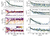 |
Fig. 15. Radial profiles of galaxies, galaxy properties, and physical properties of the underlying dark matter, gas, and stars, centered on the most massive halo in the zFIRE protocluster region. Left: Median distribution of the number of surrounding galaxies, plus their sSFR, gas fraction, and ⟨g − r⟩ color, including galaxies with M⋆ > 108 M⊙. The virial radii of the main zFIRE halo are indicated by the vertical dashed lines. Right, top panel: Radial density profiles for dark matter, gas, and stars. Right, bottom three panels: Neutral hydrogen density, temperature, and metallicity radial profiles. Each colored line shows another variation run, while the black line shows their median. |
In the left panels of Fig. 15, only galaxies with stellar masses above 108 M⊙ are included. We find strong trends of their specific star formation rate and gas fraction as a function of distance from the protocluster center, clearly signaling the impact of environmental effects, even beyond the virial radius of the central protocluster halo (vertical dashed lines). Galaxies within this boundary are, on average, less star-forming, often quenched, and significantly gas depleted. Although the median sSFR and fgas decreases toward the protocluster center, we simultaneously find an increased number of gas-rich and rapidly star-forming galaxies, typically with low masses 108 − 109 M⊙. This overall change in star formation is just weakly imprinted in the ⟨g − r⟩ color with an 0.1 mag increase from the overall median of ⟨g − r⟩∼0.1 mag. Such outliers may indicate peculiar environmental effects such as the enhancement of SFR due to compression of the star-forming interstellar medium (Vulcani et al. 2018; Göller et al. 2023). A detailed comparison of how galaxies evolve in the particular environments of the zFIRE and Hyperion protoclusters, and how this evolution differs from typical environmental effects at the same overdensity, will be explored in future work.
The right panels of Fig. 15 reveal that the large-scale mass distribution of dark matter and gas is similar between the eight variation runs, out to several Mpc. The stellar density field shows the most variation, due to the varying positions of individual high stellar mass systems. Variation in the neutral hydrogen density, as well as gas temperature, reflect the strong impact of baryonic feedback effects, including stellar and AGN-driven outflows, as well as the impact of the AGN radiation field. Of particular interest, these differences will be reflected in the observables of Lyman-alpha, including halo-scale and cosmic web-scale emission (Byrohl et al. 2021; Byrohl & Nelson 2023), as well as absorption in the forest as used in the reconstruction of the underlying density field for the constrained initial conditions. Both topics, in the particular environments of the COSMOS field, will be the subject of future work.
3.8. Galaxy clustering
We close by extending our analysis beyond one-point statistics, to better understand the spatial distribution of galaxies and their clustering in cosmosTNG. Figure 16 shows the projected two-point correlation function of ω(r) for cosmosTNG and TNG100 at z ∼ 2.73 for galaxies with stellar masses above 1010.0 M⊙. We compute the projected correlation function with a line-of-sight integration limit of πmax = 20 cMpc/h as
 (1)
(1)
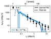 |
Fig. 16. Projected two-point correlation function for galaxies with stellar masses above 1010.0 M⊙ at z = 2.73 in cosmosTNG and TNG100. We show observational data with the same mass cut for ⟨z⟩ = 2.8 from Durkalec et al. (2018). |
using the Landy-Szalay estimator for the underlying correlation function ξ(rp,π) (Landy & Szalay 1993).
There is a mild clustering excess in cosmosTNG compared to TNG100, particularly at smaller scales. The clustering signal in cosmosTNG quickly drops off above rp ≥ 3 cMpc/h due to the limited plane of the sky extent of the simulated volume. For comparison, we show observations for the clustering of galaxies above the same mass threshold at ⟨z⟩∼2.8 from Durkalec et al. (2018). Both TNG simulations are consistent with the observed clustering signal. This improves over earlier comparisons of cluster in COSMOS with theoretical models (e.g., McCracken et al. 2007). Due to our limited redshift depth, we cannot compare to projected clustering measurements based on photometric redshifts. However, in addition to the prominent zFIRE and Hyperion protocluster regions, clustering algorithms have recently enabled robust catalogs of galaxy assemblies down to the group mass scale, and out to z ≳ 2 (Toni et al. 2024), which we can use to further explore the impact of environment and environmental effects on galaxy evolution in the COSMOS field.
4. Discussion and future prospects
4.1. Constrained simulations at cosmic noon
Galaxy properties are shaped by their large-scale environment, and interactions in dense environments are an important influence for the galaxy population. Constrained cosmological simulations are an important tool to understand and test our galaxy formation models in this aspect. In the local universe at z ∼ 0 they directly probe the assembly of observed clusters and their galaxies. At high redshift, galaxies evolve even more rapidly, and have more frequent interactions, and constrained simulations similarly enable us to study the vigorous star formation and merger activity at cosmic noon.
Constrained cosmological simulations are complementary to conventional cosmological galaxy formation simulations using random realizations for the initial conditions. First, they enable a more meaningful and direct comparison with observational surveys in the reconstructed volumes, given that the large-scale structure matches, minimizing biases from cosmic variance. Second, constrained simulations allow us to investigate the biases and nonlinear relations between different observed tracers. Specifically, we have knowledge of both the diffuse gas distribution (Lyα forest) and bright star-forming galaxies (via photometric and spectroscopic surveys) in the COSMOS field. As a result, we can assess how well the constrained simulation agrees with different observed tracers.
The resulting (dis)agreement reflects how well a given field, observable, or galaxy population traces the underlying matter density field (e.g., Momose et al. 2024). Simultaneously, it provides a somewhat new vantage point onto the evaluation of the fidelity of the underlying galaxy formation model. These two effects are partially degenerate, but one could vary the information (i.e., tracer(s) used during the reconstruction procedure) in order to differentiate their relative roles. Such an approach may be particularly insightful at high redshifts, contrasting absorption from HI in the Lyα forest versus galaxy population observations, where the relationship and connections between the two may be nontrivial.
Constrained simulations at the epoch of z ∼ 2 cosmic noon provide further practical advantages: notably, the availability of Lyman-alpha forest tomography for mapping the diffuse gas large-scale structure (Lee et al. 2014b). Computationally, the compute time requirement is also only 20% of an analogous simulation run all the way to z = 0. In the present work, this has enabled us to run the eight variations of the same volume, in order to better marginalize over unconstrained small-scale structure.
4.2. Uniqueness of the cosmosTNG target region
CLAMATO and the cosmosTNG volume target an overdense region, as indicated by the excess of massive halos in the HMF (see Fig. A.1). Part of this can already be seen in the initial conditions (Fig. 3) showing an excess in power on constrained large spatial scales between k = 0.2 and 1 h/cMpc. This excess could be partly physical, related to the specific constrained field, and partly related to the TARDIS pipeline (see, e.g., Fig. 4 in Horowitz et al. 2021).
To better understand the region, we quantify the uniqueness of the cosmosTNG subvolume in terms of the number density of massive halos with Mh > 1013 M⊙. We compare the mean value of different realizations to the probability density function inferred from the much larger, dark matter-only cosmological simulation Millennium (Springel et al. 2005). The result is shown in Fig. 17. This probability distribution is computed by randomly sampling subvolumes of Millennium (boxsize 500 cMpc3/h3) with the cosmosTNG geometry and computing the number of massive halos each contains (blue distribution). As we have selected the cosmosTNG subvolume given the presence of the zFIRE protocluster, we also repeat this procedure under the constraint of one such massive halo is present at the same relative position as in cosmosTNG (orange distribution). This is done by first selecting massive halos in Millennium and centering the masking volume by the offset between zFIRE and the cosmosTNG subvolume center.
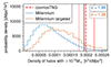 |
Fig. 17. Assessment of the rarity of the cosmosTNG volume. Specifically, we randomly place cosmosTNG subvolumes within the Millennium-I simulation, and measure the number density of halos with Mh > 1013 M⊙. The probability density for many random subvolumes (blue) is contrasted against the same, but for volumes with a Mh > 1013 M⊙ halo at the relative position of the zFIRE cluster within cosmosTNG (orange). The vertical red lines show the number density measured within the cosmosTNG variation runs, and the dashed line shows their mean. |
We find standard deviations of σ = 1.9 (σ = 1.4) for the cosmosTNG subvolume when compared against a random (targeted) realization, demonstrating that the cosmosTNG volume is a considerably overdense environment. Such an environment is not present in conventional cosmological simulations using random realizations at the resolution studied here, including TNG100. We note that the standard deviation is approximate given the differing cosmologies of cosmosTNG and Millennium.
4.3. Galaxy evolution modulated by large-scale structure
Using the TNG galaxy model and comparing to a fiducial realization in TNG100, we find significant changes in many summary statistics presented in Sect. 3. These include: an early peaking of the cosmic star formation rate density, an enhancement in the stellar mass function at the high-mass end, a stellar-mass shift of the quenched fraction, and a mild clustering excess.
These findings are qualitatively consistent with the presence of more pronounced large-scale overdensities (Sect. 4.2), most prominently the zFIRE galaxy protocluster at z ≈ 2.1. In particular, observations suggest that large-scale overdensities modulate the normalization of the stellar mass function, and in doing so over-proportionally enhance the number density of massive galaxies (Daikuhara et al. 2024; Forrest et al. 2024a). Curiously, we also find a shift of the quenched fraction as a function of stellar mass toward higher galaxy masses, corresponding to a mildly lower quenched fraction at fixed mass (Fig. 10) when compared to the TNG100 simulation. This is one of the most striking differences in cosmosTNG with respect to other TNG model simulations. It suggests that the particular large-scale environment of the COSMOS field has a strong and observable impact on the history and/or frequency of galaxy quenching.
In order to better understand the robustness and consistency of such differences, we ran eight variations of the same simulation volume. All have the large-scale density field fixed by the TARDIS constraints, but randomly inject power for k ≥ 1 h/cMpc where observational constraints are missing. Overall, we find only limited variance in outcomes caused by the random modes for various galaxy summary statistics such as the SMF, the SFRD, and the clustering signal. Only at high masses do significant variations start to appear due to low number statistics of the underlying massive halos and their more nonlinear nature. Variation-to-variation differences are smaller than the difference of cosmosTNG to TNG100. This suggests that the large-scale density field (i.e., modes at k > 1 h/cMpc) have a strong and overwhelming impact on galaxy population statistics and scaling relations at this level.
On the scale of individual protocluster regions (Sect. 3.7), however, substantial variations arise. While the density profiles are similar, protohalo masses (Table 2) and their temperature and metallicity profiles (Fig. 14) often vary by a factor of 2 or more. This indicates the lack of small-scale power constraints as well as constraints on the formation history of these regions.
The TARDIS pipeline imposes no strong cosmological constraints on the field reconstruction, even though its forward model evolves the fields at fixed cosmology (Horowitz et al. 2021, 2022). The resulting power excess on large scales (Fig. 3) might in parts indicate the uniqueness of the simulated COSMOS subvolume as an overdense field, as well as an underestimated bias of the hydrogen Lyman-α optical depth. Furthermore, the TARDIS pipeline itself has shown to introduce excess power on intermediate constrained scales (see Horowitz et al. 2021). This potential uniqueness moreover implies that caution should be exercised when interpreting the observed 2 ≲ z ≲ 2.5 galaxy properties from surveys that have significant overlap with the CLAMATO field (Fig. 1), such as COSMOS-Web (Casey et al. 2023). There are also possible ramifications toward cosmological surveys due to the heavy dependence on the COSMOS field for calibrating photometric redshifts (e.g., Masters et al. 2017); further analysis might be required on the full ∼1 deg2 COSMOS field to check whether overdensities might be biasing these calibrations.
4.4. Reconstruction methods and future directions
The initial conditions, particularly Fourier modes on resolved, reconstructed scales k ≤ 1 h/Mpc, can strongly affect the observed properties of frequently studied massive galaxies. We now discuss shortcomings and future directions for the reconstruction pipeline and use in cosmological galaxy formation simulations.
The cosmosTNG simulations are run as a downstream step following reconstruction using the TARDIS inference scheme applied on joint Lyman-α forest and galaxy redshift data sets. Ultimately, we would want to integrate galaxy formation simulations within the reconstruction pipeline. This would enable an ‘end-to-end’ forward model, at the level of galaxy observables, or even at the field level. However, key challenges exist in this regard. First, the current likelihood maximization method makes use of the differentiability of its forward model. Despite recent progress (Li et al. 2024), this remains out-of-reach for complex galaxy formation simulation models such as TNG. Furthermore, the computational costs would certainly be prohibitive, without model surrogate or emulation techniques. In the interim, future work can aim to increase consistency between the expensive downstream galaxy formation simulations and the cheap reconstruction forward model.
A major improvement to the reconstruction scheme will stem from an improved treatment and coupling of the two complementary tracers used in this study, namely diffuse gas traced by the Lyα forest and bright star-forming galaxy populations. Both are subject to different biases and modeling uncertainties. In the TARDIS-based reconstruction applied here, bright galaxies from the zCOSMOS survey and Lyα absorption from the CLAMATO survey were used simultaneously, even though the former generally influences only the overall amplitude of the reconstruction and not the detailed filamentary structure (Horowitz et al. 2021).
As such, we are particularly susceptible to systematics in the mapping of observed Lyα forest to the underlying density field. In the reconstruction, the TARDIS scheme assumes the FGPA, which becomes increasingly inconsistent with the hydrodynamical result at redshift z ∼ 2 (Kooistra et al. 2022). Recent observations indicate that in some cases galaxies and Lyα forest do not just not trace each other, but are even anti-correlated. For example, Dong et al. (2023) found that some Lyα forest reconstructed underdensities host overdensities in galaxies, while Newman et al. (2022) found environments with the opposite relation, where overdense neutral hydrogen regions are underdense in galaxies.
Future explorations with cosmosTNG will revisit the Lyα forest in cosmosTNG, studying its deviations from the FGPA and potential protocluster heating around massive objects, to be parameterized in the forward model (Horowitz et al. 2021). As we have shown, when we can faithfully map the Lyα forest to the underlying matter field, the large-scale overdensities encoded in the initial conditions lead to the spatially coherent emergence of massive protocluster regions below the reconstruction scale (see Fig. 14). This might indicate an underrepresented relative weight of massive galaxies in the reconstruction pipeline.
Current and upcoming data from surveys such as JWST PRIMER, COSMOS-Web, Blue Jay, and COSMOS-3D (Dunlop et al. 2021; Casey et al. 2023; Belli et al. 2024; Kakiichi et al. 2024) in the field will not only allow a better comparison with simulation outcomes, but will add a substantial constraint above the current cutoff scale of k ≳ 1 h/cMpc. For example, the protohalo studied in Sect. 3.7 is currently only covered by a few zCOSMOS galaxies. Hence, much of the information provided by the distribution of shown zFIRE galaxies is currently missing, which can be included along with other survey data in future reconstructions. The reconstruction can further benefit from additional tracers (i.e., orthogonal probes) other than Lyα forest and galaxies, such as the cosmic web Lyα emission (Bacon et al. 2021; Byrohl & Nelson 2023; Martin et al. 2023).
We have also only simulated a partial region of the reconstructed CLAMATO field (Fig. 4) in this work. Extensions of cosmosTNG toward other parts of the field, for example the large cosmic void at z ≈ 2.35 Krolewski et al. (2018); see top panels of Fig. 4) could reveal interesting astrophysics.
5. Conclusions
In this introductory paper we presented the new cosmosTNG simulation suite. This is a set of cosmological galaxy formation simulations run with the IllustrisTNG model and with constrained initial conditions inferred from the galaxy and gas distribution within the COSMOS field, evolved to cosmic noon at z = 2. We compared our results to the TNG100 simulation with conventional random initial conditions, and to observations across a variety of galaxy properties, including star formation rates, quenching, supermassive black hole masses, environmental effects, and clustering.
Our main findings are the following:
-
The reconstructed initial conditions, evolved with the TNG galaxy formation model, give broadly consistent results with the TNG100 cosmological galaxy formation simulation. Simultaneously, the distribution of simulated galaxies at z ∼ 2 is roughly and qualitatively consistent with the observed (α, δ, z) distribution of galaxies from spectroscopic surveys.
-
At the high-mass end, cosmosTNG shows key differences with respect to a random realization. Most notably, it has an enhanced number of halos and galaxies (i.e., a greater number of high stellar mass galaxies than expected, ∼2× for M⋆ ≥ 1011 M⊙), qualitatively consistent with excess power in the constrained volume. These systems have an overall increased star formation activity and a lower quenched fraction in comparison to TNG100 (Δq. frac. ∼ 20% at M⋆ = 1011 M⊙).
-
The abundance of massive galaxies at 2 < z < 5 is in reasonable agreement with observational inferences. The abundance of massive quiescent galaxies is low, potentially lower than observations suggest, although the volume of cosmosTNG is too limited to draw stronger conclusions.
-
cosmosTNG shows an intriguing signal in the relationship between supermassive black hole (SMBH) and galaxy stellar mass, as suggested by recent JWST observations. In particular, with respect to the local z = 0 relation, cosmosTNG galaxies host overmassive black holes, by ∼0.5 dex at 2 ≲ z ≲ 4. While this average difference largely vanishes at z > 4, we show that lower mass galaxies with M⋆ ∼ 109 M⊙ can have SMBHs overmassive by up to 2 dex up to z = 5.
-
The properties of galaxies and of the underlying dark matter, gas, and stellar matter fields around the zFIRE protocluster hint toward unique imprints of environmental effects on galaxy evolution in this region, while showing a qualitatively consistent large-scale structure on the reconstruction scale (k = 1 h/cMpc).
Our results show notable differences for galaxy properties at the high-mass end > 1011 M⊙, demonstrating the need for caution for assessing the simulation’s realism or their astrophysical and cosmological implications when contrasted with observed high-redshift survey volumes. Future analyses will focus on further comparing the observed properties of galaxies specifically within the COSMOS region to simulated outcomes, enabling a new theoretical vantage point on galaxy formation and environmental effects on galaxy evolution at cosmic noon.
6. Data availability
The cosmosTNG simulations will be made publicly available and accessible at https://www.tng-project.org/data/ (Nelson et al. 2019b) in the near future. Data directly related to this publication is available on request from the corresponding author.
In the current reconstruction, we find that zCOSMOS galaxies play only a minor role for the resulting initial conditions.
Along the redshift direction, only the first 438 cMpc/h cover the constrained CLAMATO redshift range z = 2.05 − 2.55.
This is a minor difference in the cosmology used for FlowPM and AREPO compared to these conversion factors, in order to be consistent with the CLAMATO data release.
Acknowledgments
All of our post-processing and analysis of the simulations makes use the scida analysis library (Byrohl & Nelson 2024). CB and DN acknowledge funding from the Deutsche Forschungsgemeinschaft (DFG) through an Emmy Noether Research Group (grant number NE 2441/1-1). We also thank the Hector Fellow Academy for their funding support. This work was further supported by the Deutsche Forschungsgemeinschaft (DFG, German Research Foundation) under Germany’s Excellence Strategy EXC 2181/1 – 390900948 (the Heidelberg STRUCTURES Excellence Cluster). This research was supported in part by grant NSF PHY-1748958 to the Kavli Institute for Theoretical Physics (KITP). The authors gratefully acknowledge the scientific support and HPC resources provided by the Erlangen National High Performance Computing Center (NHR@FAU) of the Friedrich-Alexander-Universität Erlangen-Nürnberg (FAU) under the NHR project a103bc. NHR funding is provided by federal and Bavarian state authorities. NHR@FAU hardware is partially funded by the German Research Foundation (DFG) – 440719683. Additional simulations and analysis were carried out on the Vera machine of the Max Planck Institute for Astronomy (MPIA) and systems at the Max Planck Computing and Data Facility (MPCDF). KGL acknowledges support from JSPS Kakenhi Grant JP24H00241. Kavli IPMU is supported by the World Premier International Research Center Initiative (WPI), MEXT, Japan.
References
- Ata, M., Kitaura, F.-S., Lee, K.-G., et al. 2021, MNRAS, 500, 3194 [Google Scholar]
- Ata, M., Lee, K.-G., Vecchia, C. D., et al. 2022, Nat. Astron., 6, 857 [NASA ADS] [CrossRef] [Google Scholar]
- Bacon, R., Mary, D., Garel, T., et al. 2021, A&A, 647, A107 [NASA ADS] [CrossRef] [EDP Sciences] [Google Scholar]
- Belli, S., Park, M., Davies, R. L., et al. 2024, Nature, 630, 54 [NASA ADS] [CrossRef] [Google Scholar]
- Bennert, V. N., Auger, M. W., Treu, T., Woo, J.-H., & Malkan, M. A. 2011, ApJ, 726, 59 [NASA ADS] [CrossRef] [Google Scholar]
- Bogdán, Á., Goulding, A. D., Natarajan, P., et al. 2024, Nat. Astron., 8, 126 [Google Scholar]
- Bond, J. R., Kofman, L., & Pogosyan, D. 1996, Nature, 380, 603 [NASA ADS] [CrossRef] [Google Scholar]
- Bouwens, R. J., Illingworth, G. D., Oesch, P. A., et al. 2015, ApJ, 803, 34 [Google Scholar]
- Byrohl, C., & Nelson, D. 2023, MNRAS, 523, 5248 [NASA ADS] [CrossRef] [Google Scholar]
- Byrohl, C., & Nelson, D. 2024, J. Open Source Softw., 9, 6064 [NASA ADS] [CrossRef] [Google Scholar]
- Byrohl, C., Nelson, D., Behrens, C., et al. 2021, MNRAS, 506, 5129 [NASA ADS] [CrossRef] [Google Scholar]
- Capak, P., Aussel, H., Ajiki, M., et al. 2007, ApJS, 172, 99 [Google Scholar]
- Carnall, A. C., Walker, S., McLure, R. J., et al. 2020, MNRAS, 496, 695 [Google Scholar]
- Carnall, A. C., McLeod, D. J., McLure, R. J., et al. 2023, MNRAS, 520, 3974 [NASA ADS] [CrossRef] [Google Scholar]
- Casey, C. M., Kartaltepe, J. S., Drakos, N. E., et al. 2023, ApJ, 954, 31 [NASA ADS] [CrossRef] [Google Scholar]
- Caucci, S., Colombi, S., Pichon, C., et al. 2008, MNRAS, 386, 211 [Google Scholar]
- Costantin, L., Pérez-González, P. G., Vega-Ferrero, J., et al. 2023, ApJ, 946, 71 [NASA ADS] [CrossRef] [Google Scholar]
- Cucciati, O., Tresse, L., Ilbert, O., et al. 2012, A&A, 539, A31 [NASA ADS] [CrossRef] [EDP Sciences] [Google Scholar]
- Daikuhara, K., Kodama, T., Pérez-Martínez, J. M., et al. 2024, MNRAS, 531, 2335 [NASA ADS] [CrossRef] [Google Scholar]
- Darvish, B., Mobasher, B., Martin, D. C., et al. 2017, ApJ, 837, 16 [Google Scholar]
- Davidzon, I., Ilbert, O., Laigle, C., et al. 2017, A&A, 605, A70 [NASA ADS] [CrossRef] [EDP Sciences] [Google Scholar]
- Dekel, A., Birnboim, Y., Engel, G., et al. 2009, Nature, 457, 451 [Google Scholar]
- Dolag, K., Sorce, J. G., Pilipenko, S., et al. 2023, A&A, 677, A169 [NASA ADS] [CrossRef] [EDP Sciences] [Google Scholar]
- Dong, C., Lee, K.-G., Ata, M., Horowitz, B., & Momose, R. 2023, ApJ, 945, L28 [NASA ADS] [CrossRef] [Google Scholar]
- Dong, C., Lee, K.-G., Cui, W., Davé, R., & Sorini, D. 2024, MNRAS, 532, 4876 [Google Scholar]
- Donnari, M., Pillepich, A., Nelson, D., et al. 2019, MNRAS, 485, 4817 [Google Scholar]
- Donnari, M., Pillepich, A., Nelson, D., et al. 2021, MNRAS, 506, 4760 [NASA ADS] [CrossRef] [Google Scholar]
- Du, M., Ma, H.-C., Zhong, W.-Y., et al. 2024, A&A, 686, A168 [NASA ADS] [CrossRef] [EDP Sciences] [Google Scholar]
- Dunlop, J. S., Abraham, R. G., Ashby, M. L. N., et al. 2021, JWST Proposal. Cycle 1, 1837 [Google Scholar]
- Durkalec, A., Le Fèvre, O., Pollo, A., et al. 2018, A&A, 612, A42 [NASA ADS] [CrossRef] [EDP Sciences] [Google Scholar]
- Edward, A. H., Balogh, M. L., Bahé, Y. M., et al. 2024, MNRAS, 527, 8598 [Google Scholar]
- Enia, A., Talia, M., Pozzi, F., et al. 2022, ApJ, 927, 204 [NASA ADS] [CrossRef] [Google Scholar]
- Faucher-Giguère, C.-A., Lidz, A., Zaldarriaga, M., & Hernquist, L. 2009, ApJ, 703, 1416 [Google Scholar]
- Feng, Y., Chu, M.-Y., Seljak, U., & McDonald, P. 2016, MNRAS, 463, 2273 [NASA ADS] [CrossRef] [Google Scholar]
- Finkelstein, S. L., Bagley, M. B., Ferguson, H. C., et al. 2023, ApJ, 946, L13 [NASA ADS] [CrossRef] [Google Scholar]
- Forrest, B., Lemaux, B. C., Shah, E. A., et al. 2024a, ApJ, 971, 169 [NASA ADS] [Google Scholar]
- Forrest, B., Cooper, M. C., Muzzin, A., et al. 2024b, ApJ, 977, 51 [Google Scholar]
- Garaldi, E., Kannan, R., Smith, A., et al. 2022, MNRAS, 512, 4909 [NASA ADS] [CrossRef] [Google Scholar]
- Genel, S., Vogelsberger, M., Springel, V., et al. 2014, MNRAS, 445, 175 [Google Scholar]
- Genel, S., Nelson, D., Pillepich, A., et al. 2018, MNRAS, 474, 3976 [Google Scholar]
- Göller, J., Joshi, G. D., Rohr, E., Zinger, E., & Pillepich, A. 2023, MNRAS, 525, 3551 [CrossRef] [Google Scholar]
- Gottloeber, S., Hoffman, Y., & Yepes, G. 2010, arXiv e-prints [arXiv:1005.2687] [Google Scholar]
- Gould, K. M. L., Brammer, G., Valentino, F., et al. 2023, ApJ, 165, 248 [Google Scholar]
- Greene, J., Bezanson, R., Ouchi, M., Silverman, J., & the PFS Galaxy Evolution Working Group 2022, arXiv e-prints [arXiv:2206.14908] [Google Scholar]
- Gruppioni, C., Pozzi, F., Rodighiero, G., et al. 2013, MNRAS, 432, 23 [Google Scholar]
- Gupta, A., Tran, K.-V., Pillepich, A., et al. 2021, ApJ, 907, 95 [Google Scholar]
- Harikane, Y., Zhang, Y., Nakajima, K., et al. 2023, ApJ, 959, 39 [NASA ADS] [CrossRef] [Google Scholar]
- Häring, N., & Rix, H.-W. 2004, ApJ, 604, L89 [Google Scholar]
- Hasinger, G., Capak, P., Salvato, M., et al. 2018, ApJ, 858, 77 [Google Scholar]
- Hopkins, P. F., Richards, G. T., & Hernquist, L. 2007, ApJ, 654, 731 [Google Scholar]
- Hopkins, P. F., Wetzel, A., Kereš, D., et al. 2018, MNRAS, 480, 800 [NASA ADS] [CrossRef] [Google Scholar]
- Horowitz, B., Lee, K.-G., White, M., Krolewski, A., & Ata, M. 2019, ApJ, 887, 61 [NASA ADS] [CrossRef] [Google Scholar]
- Horowitz, B., Zhang, B., Lee, K.-G., & Kooistra, R. 2021, ApJ, 906, 110 [Google Scholar]
- Horowitz, B., Lee, K.-G., Ata, M., et al. 2022, ApJS, 263, 27 [NASA ADS] [CrossRef] [Google Scholar]
- Ilbert, O., Capak, P., Salvato, M., et al. 2009, ApJ, 690, 1236 [NASA ADS] [CrossRef] [Google Scholar]
- Ilbert, O., McCracken, H. J., Le Fèvre, O., et al. 2013, A&A, 556, A55 [NASA ADS] [CrossRef] [EDP Sciences] [Google Scholar]
- Ilbert, O., Arnouts, S., Le Floc’h, E., et al. 2015, A&A, 579, A2 [NASA ADS] [CrossRef] [EDP Sciences] [Google Scholar]
- Ji, Z., Williams, C. C., Suess, K. A., et al. 2024, ApJ, submitted [arXiv:2401.00934] [Google Scholar]
- Kakiichi, K., Egami, E., Fan, X., et al. 2024, JWST Proposal. Cycle 3, 5893 [Google Scholar]
- Kannan, R., Garaldi, E., Smith, A., et al. 2022, MNRAS, 511, 4005 [NASA ADS] [CrossRef] [Google Scholar]
- Karmakar, T., Genel, S., & Somerville, R. S. 2023, MNRAS, 520, 1630 [NASA ADS] [CrossRef] [Google Scholar]
- Kitaura, F.-S., Ata, M., Rodríguez-Torres, S. A., et al. 2021, MNRAS, 502, 3456 [NASA ADS] [CrossRef] [Google Scholar]
- Kooistra, R., Lee, K.-G., & Horowitz, B. 2022, ApJ, 938, 123 [NASA ADS] [CrossRef] [Google Scholar]
- Kriek, M., Shapley, A. E., Reddy, N. A., et al. 2015, ApJS, 218, 15 [NASA ADS] [CrossRef] [Google Scholar]
- Krolewski, A., Lee, K.-G., White, M., et al. 2018, ApJ, 861, 60 [Google Scholar]
- Lacey, C., & Cole, S. 1993, MNRAS, 262, 627 [NASA ADS] [CrossRef] [Google Scholar]
- Laigle, C., McCracken, H. J., Ilbert, O., et al. 2016, ApJS, 224, 24 [Google Scholar]
- Laigle, C., Pichon, C., Arnouts, S., et al. 2018, MNRAS, 474, 5437 [Google Scholar]
- Landy, S. D., & Szalay, A. S. 1993, ApJ, 412, 64 [Google Scholar]
- Lee, K.-G., Suzuki, N., & Spergel, D. N. 2012, ApJ, 143, 51 [Google Scholar]
- Lee, K.-G., Hennawi, J. F., Stark, C., et al. 2014a, ApJ, 795, L12 [NASA ADS] [CrossRef] [Google Scholar]
- Lee, K.-G., Hennawi, J. F., White, M., Croft, R. A. C., & Ozbek, M. 2014b, ApJ, 788, 49 [NASA ADS] [CrossRef] [Google Scholar]
- Lee, K.-G., Hennawi, J. F., White, M., et al. 2016, ApJ, 817, 160 [NASA ADS] [CrossRef] [Google Scholar]
- Lee, K.-G., Krolewski, A., White, M., et al. 2018, ApJS, 237, 31 [Google Scholar]
- Lee, J., Shin, J., Snaith, O. N., et al. 2021, ApJ, 908, 11 [CrossRef] [Google Scholar]
- Le Fèvre, O., Tasca, L. A. M., Cassata, P., et al. 2015, A&A, 576, A79 [Google Scholar]
- Legrand, L., McCracken, H. J., Davidzon, I., et al. 2019, MNRAS, 486, 5468 [NASA ADS] [CrossRef] [Google Scholar]
- Leja, J., Speagle, J. S., Johnson, B. D., et al. 2020, ApJ, 893, 111 [Google Scholar]
- Leja, J., Speagle, J. S., Ting, Y.-S., et al. 2022, ApJ, 936, 165 [NASA ADS] [CrossRef] [Google Scholar]
- Lewis, A., Challinor, A., & Lasenby, A. 2000, ApJ, 538, 473 [Google Scholar]
- Li, R., Wang, H., Mo, H. J., et al. 2022, ApJ, 936, 11 [Google Scholar]
- Li, Y., Modi, C., Jamieson, D., et al. 2024, ApJS, 270, 36 [Google Scholar]
- Libeskind, N. I., Carlesi, E., Grand, R. J. J., et al. 2020, MNRAS, 498, 2968 [NASA ADS] [CrossRef] [Google Scholar]
- Lilly, S. J., Le Fèvre, O., Renzini, A., et al. 2007, ApJS, 172, 70 [Google Scholar]
- Liu, D. C., & Nocedal, J. 1989, Math. Program., 45, 503 [CrossRef] [Google Scholar]
- Luo, X., Wang, H., Cui, W., et al. 2024, ApJ, 966, 236 [Google Scholar]
- Madau, P., & Dickinson, M. 2014, ARA&A, 52, 415 [Google Scholar]
- Magnelli, B., Elbaz, D., Chary, R. R., et al. 2011, A&A, 528, A35 [NASA ADS] [CrossRef] [EDP Sciences] [Google Scholar]
- Magnelli, B., Popesso, P., Berta, S., et al. 2013, A&A, 553, A132 [NASA ADS] [CrossRef] [EDP Sciences] [Google Scholar]
- Maiolino, R., Cirasuolo, M., Afonso, J., et al. 2020, Messenger, 180, 24 [Google Scholar]
- Maiolino, R., Scholtz, J., Witstok, J., et al. 2024, Nature, 627, 59 [NASA ADS] [CrossRef] [Google Scholar]
- Marinacci, F., Vogelsberger, M., Pakmor, R., et al. 2018, MNRAS, 480, 5113 [NASA ADS] [Google Scholar]
- Martin, D. C., Darvish, B., Lin, Z., et al. 2023, Nat. Astron., 7, 1390 [NASA ADS] [CrossRef] [Google Scholar]
- Masters, D. C., Stern, D. K., Cohen, J. G., et al. 2017, ApJ, 841, 111 [Google Scholar]
- McAlpine, S., Helly, J. C., Schaller, M., et al. 2022, MNRAS, 512, 5823 [CrossRef] [Google Scholar]
- McCracken, H. J., Peacock, J. A., Guzzo, L., et al. 2007, ApJS, 172, 314 [NASA ADS] [CrossRef] [Google Scholar]
- McCracken, H. J., Wolk, M., Colombi, S., et al. 2015, MNRAS, 449, 901 [NASA ADS] [CrossRef] [Google Scholar]
- Merlin, E., Fortuni, F., Torelli, M., et al. 2019, MNRAS, 490, 3309 [CrossRef] [Google Scholar]
- Modi, C., Chen, S.-F., & White, M. 2020, MNRAS, 492, 5754 [NASA ADS] [CrossRef] [Google Scholar]
- Modi, C., Lanusse, F., & Seljak, U. 2021, Astron. Comput., 37, 100505 [NASA ADS] [CrossRef] [Google Scholar]
- Momose, R., Lee, K.-G., Ata, M., Horowitz, B., & Kartaltepe, J. S. 2024, PASJ, 76, 1143 [Google Scholar]
- Moustakas, J., Coil, A. L., Aird, J., et al. 2013, ApJ, 767, 50 [NASA ADS] [CrossRef] [Google Scholar]
- Muzzin, A., Marchesini, D., Stefanon, M., et al. 2013, ApJ, 777, 18 [NASA ADS] [CrossRef] [Google Scholar]
- Naiman, J. P., Pillepich, A., Springel, V., et al. 2018, MNRAS, 477, 1206 [Google Scholar]
- Nanayakkara, T., Glazebrook, K., Kacprzak, G. G., et al. 2016, ApJ, 828, 21 [NASA ADS] [CrossRef] [Google Scholar]
- Nedkova, K. V., Häußler, B., Marchesini, D., et al. 2021, MNRAS, 506, 928 [NASA ADS] [CrossRef] [Google Scholar]
- Nelson, D., Pillepich, A., Springel, V., et al. 2018, MNRAS, 475, 624 [Google Scholar]
- Nelson, D., Pillepich, A., Springel, V., et al. 2019a, MNRAS, 490, 3234 [Google Scholar]
- Nelson, D., Springel, V., Pillepich, A., et al. 2019b, Comput. Astrophys. Cosmol., 6, 2 [Google Scholar]
- Nelson, D., Pillepich, A., Ayromlou, M., et al. 2024, A&A, 686, A157 [NASA ADS] [CrossRef] [EDP Sciences] [Google Scholar]
- Newman, A. B., Rudie, G. C., Blanc, G. A., et al. 2020, ApJ, 891, 147 [NASA ADS] [CrossRef] [Google Scholar]
- Newman, A. B., Rudie, G. C., Blanc, G. A., et al. 2022, Nature, 606, 475 [NASA ADS] [CrossRef] [Google Scholar]
- Pakmor, R., Bauer, A., & Springel, V. 2011, MNRAS, 418, 1392 [NASA ADS] [CrossRef] [Google Scholar]
- Pakmor, R., Springel, V., Coles, J. P., et al. 2023, MNRAS, 524, 2539 [NASA ADS] [CrossRef] [Google Scholar]
- Park, M., Belli, S., Conroy, C., et al. 2024, arXiv e-prints [arXiv:2404.17945] [Google Scholar]
- Peng, Y.-j., Lilly, S. J., Kovač, K., et al. 2010, ApJ, 721, 193 [NASA ADS] [CrossRef] [Google Scholar]
- Pichon, C., Vergely, J. L., Rollinde, E., Colombi, S., & Petitjean, P. 2001, MNRAS, 326, 597 [Google Scholar]
- Pillepich, A., Springel, V., Nelson, D., et al. 2018a, MNRAS, 473, 4077 [Google Scholar]
- Pillepich, A., Nelson, D., Hernquist, L., et al. 2018b, MNRAS, 475, 648 [Google Scholar]
- Pillepich, A., Nelson, D., Springel, V., et al. 2019, MNRAS, 490, 3196 [Google Scholar]
- Planck Collaboration I. 2016, A&A, 594, A1 [NASA ADS] [CrossRef] [EDP Sciences] [Google Scholar]
- Porqueres, N., Jasche, J., Lavaux, G., & Enßlin, T. 2019, A&A, 630, A151 [NASA ADS] [CrossRef] [EDP Sciences] [Google Scholar]
- Porqueres, N., Hahn, O., Jasche, J., & Lavaux, G. 2020, A&A, 642, A139 [NASA ADS] [CrossRef] [EDP Sciences] [Google Scholar]
- Reddy, N. A., & Steidel, C. C. 2009, ApJ, 692, 778 [Google Scholar]
- Sawala, T., McAlpine, S., Jasche, J., et al. 2022, MNRAS, 509, 1432 [Google Scholar]
- Schaye, J., Kugel, R., Schaller, M., et al. 2023, MNRAS, 526, 4978 [NASA ADS] [CrossRef] [Google Scholar]
- Scoville, N., Abraham, R. G., Aussel, H., et al. 2007, ApJS, 172, 38 [NASA ADS] [CrossRef] [Google Scholar]
- Scoville, N., Arnouts, S., Aussel, H., et al. 2013, ApJS, 206, 3 [Google Scholar]
- Shen, X., Vogelsberger, M., Nelson, D., et al. 2022, MNRAS, 510, 5560 [NASA ADS] [CrossRef] [Google Scholar]
- Sherman, S., Jogee, S., Florez, J., et al. 2020, MNRAS, 499, 4239 [Google Scholar]
- Sirko, E. 2005, ApJ, 634, 728 [NASA ADS] [CrossRef] [Google Scholar]
- Smith, A., Kannan, R., Garaldi, E., et al. 2022, MNRAS, 512, 3243 [NASA ADS] [CrossRef] [Google Scholar]
- Sorce, J. G., & Tempel, E. 2018, MNRAS, 476, 4362 [NASA ADS] [CrossRef] [Google Scholar]
- Sorce, J. G., Dubois, Y., Blaizot, J., et al. 2021, MNRAS, 504, 2998 [NASA ADS] [CrossRef] [Google Scholar]
- Spitler, L. R., Labbé, I., Glazebrook, K., et al. 2012, ApJ, 748, L21 [NASA ADS] [CrossRef] [Google Scholar]
- Springel, V. 2010, MNRAS, 401, 791 [Google Scholar]
- Springel, V., & Hernquist, L. 2003, MNRAS, 339, 289 [Google Scholar]
- Springel, V., White, S. D. M., Jenkins, A., et al. 2005, Nature, 435, 629 [Google Scholar]
- Springel, V., Pakmor, R., Pillepich, A., et al. 2018, MNRAS, 475, 676 [Google Scholar]
- Sun, Y., Lyu, J., Rieke, G. H., et al. 2024, AAS, submitted [arXiv:2409.06796] [Google Scholar]
- Tanaka, T. S., Silverman, J. D., Ding, X., et al. 2025, ApJ, 979, 215 [Google Scholar]
- Toni, G., Maturi, M., Finoguenov, A., Moscardini, L., & Castignani, G. 2024, A&A, 687, A56 [NASA ADS] [CrossRef] [EDP Sciences] [Google Scholar]
- Treu, T., Roberts-Borsani, G., Bradac, M., et al. 2022, ApJ, 935, 110 [NASA ADS] [CrossRef] [Google Scholar]
- Valentino, F., Brammer, G., Gould, K. M. L., et al. 2023, ApJ, 947, 20 [NASA ADS] [CrossRef] [Google Scholar]
- van der Wel, A., Franx, M., van Dokkum, P. G., et al. 2014, ApJ, 788, 28 [Google Scholar]
- Vogelsberger, M., Genel, S., Springel, V., et al. 2014, Nature, 509, 177 [Google Scholar]
- Vogelsberger, M., Marinacci, F., Torrey, P., & Puchwein, E. 2020, Nat. Rev. Phys., 2, 42 [Google Scholar]
- Vulcani, B., Poggianti, B. M., Gullieuszik, M., et al. 2018, ApJ, 866, L25 [Google Scholar]
- Wang, H., Mo, H. J., Yang, X., et al. 2016, ApJ, 831, 164 [Google Scholar]
- Wang, T.-M., Magnelli, B., Schinnerer, E., et al. 2022, A&A, 660, A142 [NASA ADS] [CrossRef] [EDP Sciences] [Google Scholar]
- Weaver, J. R., Kauffmann, O. B., Ilbert, O., et al. 2022, ApJS, 258, 11 [NASA ADS] [CrossRef] [Google Scholar]
- Weaver, J. R., Davidzon, I., Toft, S., et al. 2023, A&A, 677, A184 [NASA ADS] [CrossRef] [EDP Sciences] [Google Scholar]
- Weinberger, R., Springel, V., Hernquist, L., et al. 2017, MNRAS, 465, 3291 [Google Scholar]
- Whitaker, K. E., Franx, M., Leja, J., et al. 2014, ApJ, 795, 104 [NASA ADS] [CrossRef] [Google Scholar]
- Yepes, G., Gottlöber, S., & Hoffman, Y. 2014, New Astron. Rev., 58, 1 [Google Scholar]
- Zel’dovich, Ya. B. 1970, A&A, 5, 84 [Google Scholar]
Appendix A: Resolution convergence
In Fig. A.1 we show the resolution convergence of cosmosTNG in the halo and stellar mass function. Resolution levels are indicated by the suffix number as defined in Table 1. For the halo mass function, we find good convergence for masses down to a resolution-dependent turnover at the low-mass end, which lies below 108.5 M⊙ for cosmosTNG-1, and proportionally larger by a factor of 8 according to the mass resolution for low-resolution runs. In contrast, the stellar mass function shows a systematic increase in the number of galaxies at fixed stellar mass with increasing resolution, with a difference of up to 0.2 dex per resolution level, in agreement with previous findings for the employed star formation model (Springel & Hernquist 2003) in cosmological volumes (Genel et al. 2014).
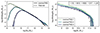 |
Fig. A.1. Resolution convergence for cosmosTNG. Left: Halo mass function (HMF) for three different resolutions. The dashed lines show the corresponding TNG100 resolution run. Right: Stellar mass function for three different resolutions and gray markers for observational data. The HMF converges down to a characteristic turnover at the low-mass end below 108.5 M⊙ for cosmosTNG-1. The cosmosTNG HMF matches well with its respective TNG100 pendant except for Mvir > 1013 M⊙ where we find an excess of massive halos in cosmosTNG. The stellar mass function generally appears to retain shape at increased resolution, but systematically increasing by up to 0.2 dex per resolution level at fixed stellar mass. |
All Tables
All Figures
|
Fig. 1. The COSMOS field and the simulated volume by cosmosTNG. The background shows HST-ACS F814W imaging of the field. We show the footprint of cosmosTNG/CLAMATO in the field, along with the zFIRE, COSMOS-Web, and PRIMER survey footprints. |
| In the text | |
|
Fig. 2. Schematic of the method. We reconstructed the initial z ∼ 100 density field from observations of zCOSMOS galaxies and CLAMATO Lyα forest measurements at z ∼ 2 using the TARDIS pipeline. We then generated constrained initial conditions using our modified version of N-GenIC, and finally ran the full hydrodynamical simulation using the AREPO code. |
| In the text | |
|
Fig. 3. Power spectrum of the simulation volume at its initial condition (z ∼ 127). Blue shows the power of the constrained field (large scales) in the 34 × 28 × 450 cMpc3/h3 volume. Orange shows the theoretically expected linear power. The shaded region shows the composite realization for the cosmosTNG simulations: modes are from the constrained field up to kcutoff = 1 h/cMpc above which we randomly draw modes according to linear theory. |
| In the text | |
|
Fig. 4. Visualization of the full constrained region evolved to z ∼ 2 from which cosmosTNG is drawn. Top: Eight consecutive projections of 4 cMpc/h thick projection of the dark matter density field showing the redshift (resp. declination) on the x-axis (resp. y-axis). Bottom: Five projections of the same dark matter density field as a function of right ascension and declination at increasing redshifts. The colored symbols show observed galaxies from spectroscopic redshift surveys. In the orange rectangles we show the zFIRE survey footprint. In the lower panel we additionally show photometric detections from the COSMOS2020 catalog as hexagons. |
| In the text | |
|
Fig. 5. Visual overview of the cosmosTNG-A simulation at z = 2. Top panel: Two 30 cMpc/h projections along the redshift direction with the right ascension (declination) on the x-axis (y-axis). On the left, we show the CLAMATO footprint, and on the right a zoomed-in view of a highly overdense region studied by the zFIRE survey. Both projections show a two-dimensional color map, where blue (red) indicates cold (hot) gas, and white (black) indicates high (low) density. The red symbols in the upper panels show observed galaxies from various spectroscopic surveys. Bottom panels: Dark matter and stellar density projections for a 10 cMpc/h thick slice through the simulation volume with the redshift (declination) on the x-axis (y-axis). Visually, we find that observed galaxies spatially correlate with the simulated density field down to the reconstruction scale of 1 cMpc/h. This correlation is particularly striking in the redshift direction within the zFIRE region, reproducing a characteristic arc shape of the galaxy distribution. |
| In the text | |
|
Fig. 6. Projections of the neutral hydrogen column density (top), temperature (middle), and metallicity (bottom) along the RA direction through the cosmosTNG-A simulation at z = 2 for a 10 cMpc/h depth with the redshift (declination) on the x-axis (y-axis). In the top panel, we also mark simulated galaxies and black holes with masses above 1010 M⊙ and 108 M⊙, respectively. Thin filaments of neutral hydrogen span the volume and at its nodes, massive galaxies reside whose AGN heat and metal-enrich their surroundings. The white box in the top panel indicates the zFIRE cluster zoomed-in region shown in Fig. 5. |
| In the text | |
|
Fig. 7. Top: Galaxy stellar mass function from cosmosTNG at redshifts z = 2, 4, 6. The semi-transparent bands span the outcomes of different variation runs with the embedded line showing the mean. In red we show the TNG100 simulation outcomes. We compare these simulations to several observational datasets (Ilbert et al. 2013; Muzzin et al. 2013; Davidzon et al. 2017; Leja et al. 2020; Weaver et al. 2023) at face value. These observations span z ∼ 2.0 − 2.5 and are shown with gray markers. In comparison to TNG100, cosmosTNG produces more high-mass galaxies above 1011 M⊙ by up to 0.5 dex. This reflects the overabundance of massive dark matter halos in this region (see text). Bottom: Relation of stellar mass to halo mass for stellar masses within the previous aperture of all central galaxies and the mass of their hosting halo at z = 2. The orange contours indicate the distribution of stellar masses at fixed halo mass across all cosmosTNG variation runs, while the individual points show galaxy outliers. The solid black (red) line shows the median stellar mass for cosmosTNG (TNG100). |
| In the text | |
|
Fig. 8. Cosmic star formation rate density (SFRD) in cosmosTNG between z = 2 − 10. The colored lines show the individual realizations, and the black line shows the average. In red we show the TNG100 simulation for comparison. Semi-transparent bands show the range contributions of different stellar mass ranges to the overall SFRD budget across different variation runs. The gray points indicate observational data from various surveys (abbrv. R09, M11, C12, M13, G13, B15 for Reddy & Steidel 2009; Magnelli et al. 2011; Cucciati et al. 2012; Magnelli et al. 2013; Gruppioni et al. 2013; Bouwens et al. 2015), with some data from Madau & Dickinson (2014), Bouwens et al. (2015). We compare this data to cosmosTNG at face value (i.e., without replicating the procedure for the observational inferences). The SFRD of cosmosTNG is overall higher, and peaks at earlier redshift, than the field result of TNG100, suggesting that z ∼ 2.1 galaxies within this region of COSMOS have undergone a particularly active assembly history. |
| In the text | |
|
Fig. 9. Size–mass relation in cosmosTNG at z = 2, combining all central galaxies regardless of type. The orange contours indicate the distribution of sizes at fixed stellar mass across all cosmosTNG variation runs, while the individual black points show outliers. The black line shows the median size at fixed stellar mass. The dashed (dotted) line shows the median at redshift z = 4 (z = 6), while the colored dashed lines show the individual variation runs. Finally, the red dots and the red line show quenched galaxies only (see text). We define galaxy size as twice the stellar half-mass radius, and here measure stellar masses summing all stellar populations within this radius. The observational data span z = 2.0 to z = 2.5 (van der Wel et al. 2014), where open symbols show early-type galaxies and filled symbols show late-type galaxies. Additionally, we show the linear scaling relations for quenched galaxies derived from observations Nedkova et al. (2021) and Ji et al. (2024) with gray lines. The observational data is compared as-is, without any further observational mock post-processing of cosmosTNG. |
| In the text | |
|
Fig. 10. Star formation activity of galaxies. Left: Specific star formation rate (sSFR) as a function of stellar mass for central galaxies in cosmosTNG at z = 2. The annotations and markers are as in Fig. 7, bottom panel. Measurements are within 2 arcsecond diameter apertures and with a 100 Myr averaged SFR. The gray markers show the inferred sSFR from observations in Whitaker et al. (2014). The dashed gray line shows the sSFR ridge from observational modeling in Leja et al. (2022). Right: Quenched fraction as a function of stellar mass in cosmosTNG and TNG100 at z = 2. The error bars show the observations from Sherman et al. (2020), Park et al. (2024) around cosmic noon. The observations are compared as-is (i.e., without reproducing the methodology used in the simulation). Quenched galaxies are defined as having a star formation rate at least 1 dex below the main sequence (see text). The colored lines show the individual realizations, and the dark solid line shows the average for all galaxies. The dashed (dotted) line shows the average for central (satellite) galaxies. A sizable population of quenched (central) galaxies with M⋆ > 1010.5 M⊙ is already present by z = 2. We see a lower quenching for cosmosTNG galaxies compared to TNG100. |
| In the text | |
|
Fig. 11. Gas fraction for all central galaxies relative to their hosting halo mass (top) and their stellar mass (bottom) in cosmosTNG at z = 2. The annotations and markers are as in Fig. 7, bottom panel. The gas and stellar mass are calculated within twice the stellar half-mass radius. We see an increased drop and scatter for gas fractions above Mhalo ≳ 1012 M⊙ and M⋆ > 1010.5 M⊙, in line with changes in the M⋆(Mhalo) and sSFR(M⋆) relations. Above these mass thresholds, cosmosTNG galaxies show a higher gas fraction on average. |
| In the text | |
|
Fig. 12. Number density of all (i.e., central and satellite) galaxies as a function of redshifts above a given stellar mass threshold in cosmosTNG-1. The shaded regions show the variation in number density across all random variations. The solid lines show the respective mean. Left: All galaxies (observational data from Weaver et al. 2023). Right: Quenched galaxies (observational data for quenched galaxy densities from Merlin et al. 2019; Carnall et al. 2020; Gould et al. 2023; Carnall et al. 2023). Observations are compared at face value without observational mock post processing of cosmosTNG. The hatched region at the bottom shows the number density 1/Vsim (i.e., one galaxy within the cosmosTNG simulation volume Vsim). |
| In the text | |
|
Fig. 13. Relation between supermassive black hole mass and galaxy stellar mass, and its evolution with time. Top: MBH–M* relation at z = 2 in cosmosTNG. The gray line shows the linear relation and the 1 − σ scatter from Tanaka et al. (2025). The annotations and markers are as in Fig. 7, bottom panel. Bottom: Evolution of the offset from the local MBH–M* relation as described in Tanaka et al. (2025) based on Häring & Rix (2004), Bennert et al. (2011) for the local relation. The points with error bars show the high-redshift observations from Harikane et al. (2023) and Tanaka et al. (2025). The gray triangles show the observations from Sun et al. (2024). All observations are compared as-is (i.e., without corrections for the respective observational methodology used when compared to cosmosTNG). The green line shows the median relation in cosmosTNG for host galaxies with M⋆ > 1011 M⊙. The shaded regions show the central 68%, 95%, and all percentiles respectively. The blue dashed line shows host galaxies with M⋆ > 108.5 M⊙. The observed galaxies with high black holes masses are rare but possible in cosmosTNG across z = 2 − 5. |
| In the text | |
|
Fig. 14. Gas density and temperature projection at z = 2 for the same comoving protocluster region across all eight variation runs in the RA–Dec plane with a projection depth of 30 cMpc/h. In the zoomed-in image in the inset, we center on the most massive halo in the proto-cluster region with a projection depth of 3 cMpc/h. The red circles indicate the halo center, and the gray crosses the mean position across variation runs. Top: Gas Density. Bottom: Temperature. We find similar density and temperature fields on the largest spatial scales. While the most massive halo appears nearly unchanged across variations, other halos seem to change substantially. |
| In the text | |
|
Fig. 15. Radial profiles of galaxies, galaxy properties, and physical properties of the underlying dark matter, gas, and stars, centered on the most massive halo in the zFIRE protocluster region. Left: Median distribution of the number of surrounding galaxies, plus their sSFR, gas fraction, and ⟨g − r⟩ color, including galaxies with M⋆ > 108 M⊙. The virial radii of the main zFIRE halo are indicated by the vertical dashed lines. Right, top panel: Radial density profiles for dark matter, gas, and stars. Right, bottom three panels: Neutral hydrogen density, temperature, and metallicity radial profiles. Each colored line shows another variation run, while the black line shows their median. |
| In the text | |
|
Fig. 16. Projected two-point correlation function for galaxies with stellar masses above 1010.0 M⊙ at z = 2.73 in cosmosTNG and TNG100. We show observational data with the same mass cut for ⟨z⟩ = 2.8 from Durkalec et al. (2018). |
| In the text | |
|
Fig. 17. Assessment of the rarity of the cosmosTNG volume. Specifically, we randomly place cosmosTNG subvolumes within the Millennium-I simulation, and measure the number density of halos with Mh > 1013 M⊙. The probability density for many random subvolumes (blue) is contrasted against the same, but for volumes with a Mh > 1013 M⊙ halo at the relative position of the zFIRE cluster within cosmosTNG (orange). The vertical red lines show the number density measured within the cosmosTNG variation runs, and the dashed line shows their mean. |
| In the text | |
|
Fig. A.1. Resolution convergence for cosmosTNG. Left: Halo mass function (HMF) for three different resolutions. The dashed lines show the corresponding TNG100 resolution run. Right: Stellar mass function for three different resolutions and gray markers for observational data. The HMF converges down to a characteristic turnover at the low-mass end below 108.5 M⊙ for cosmosTNG-1. The cosmosTNG HMF matches well with its respective TNG100 pendant except for Mvir > 1013 M⊙ where we find an excess of massive halos in cosmosTNG. The stellar mass function generally appears to retain shape at increased resolution, but systematically increasing by up to 0.2 dex per resolution level at fixed stellar mass. |
| In the text | |
Current usage metrics show cumulative count of Article Views (full-text article views including HTML views, PDF and ePub downloads, according to the available data) and Abstracts Views on Vision4Press platform.
Data correspond to usage on the plateform after 2015. The current usage metrics is available 48-96 hours after online publication and is updated daily on week days.
Initial download of the metrics may take a while.