| Issue |
A&A
Volume 697, May 2025
|
|
|---|---|---|
| Article Number | A153 | |
| Number of page(s) | 23 | |
| Section | Stellar structure and evolution | |
| DOI | https://doi.org/10.1051/0004-6361/202453554 | |
| Published online | 14 May 2025 | |
Pushing the boundaries of asteroseismic individual frequency modelling: Unveiling two evolved very low-metallicity red giants
1
Stellar Astrophysics Centre (SAC), Department of Physics and Astronomy, Aarhus University, Ny Munkegade 120, 8000 Aarhus C, Denmark
2
Aarhus Astronomy Data Centre (AADC), Department of Physics and Astronomy, Aarhus University, Ny Munkegade 120, 8000 Aarhus C, Denmark
3
DARK, Niels Bohr Institute, University of Copenhagen, Jagtvej 128, 18, 2200 Copenhagen, Denmark
4
School of Physics and Astronomy, University of Birmingham, Edgbaston B15 2TT, UK
5
Institute for Astronomy, University of Hawai‘i, 2680 Woodlawn Drive, Honolulu, HI 96822, USA
6
GRANTECAN, Cuesta de San José s/n, E-38712 Breña Baja, La Palma, Spain
7
Instituto de Astrofísica de Canarias, E-38205 La Laguna, Tenerife, Spain
8
European Southern Observatory, Alonso de Cordova 3107, Vitacura, Chile
9
Aarhus Space Centre (SpaCe), Department of Physics and Astronomy, Aarhus University, Ny Munkegade 120, 8000 Aarhus C, Denmark
10
INAF – Osservatorio Astrofisico di Catania, Via S. Sofia, 78, 95123 Catania, Italy
11
Department of Astronomical Science, School of Physical Sciences, SOKENDAI, 2-21-1 Osawa, Mitaka, Tokyo 181-8588, Japan
12
Solar Science Observatory, National Astronomical Observatory of Japan, 2-21-1 Osawa, Mitaka, Tokyo 181-8588, Japan
13
Scientific Machine Learning group, Rutherford Appleton Laboratory, Science and Technology Facilities Council, Harwell Campus, Didcot OX11 0QX, UK
14
Max-Planck-Institute for Astrophysics, Karl-Schwarzschild-Str. 1, 85748 Garching, Germany
15
LIRA, Observatoire de Paris, Université PSL, CNRS, Sorbonne Université, Université Paris-Cité, 92195 Meudon, France
16
Heidelberger Institut für Theoretische Studien, Schloss-Wolfsbrunnenweg 35, 69118 Heidelberg, Germany
17
Center for Astronomy (ZAH/LSW), Heidelberg University, Königstuhl 12, 69117 Heidelberg, Germany
18
School of Physics, University of New South Wales, Sydney, NSW 2052, Australia
19
Sydney Institute for Astronomy (SIfA), School of Physics, University of Sydney, Sydney, NSW 2006, Australia
20
ARC Centre of Excellence for All Sky Astrophysics in 3 Dimensions (ASTRO 3D), Australia
21
Division of Astronomy and Space Physics, Department of Physics and Astronomy, Uppsala University, Box 516 75120 Uppsala, Sweden
22
Independent Researcher, Münich, Germany
23
Institut für Astrophysik, Universität Wien, Türkenschanzstrasse 17, 1180 Vienna, Austria
24
Max-Planck-Institut für Sonnensystemforschung, Justus-von-Liebig-Weg 3, 37077 Göttingen, Germany
25
Lund Observatory, Department of Astronomy and Theoretical Physics, Box 43 SE-221 00 Lund, Sweden
⋆ Corresponding authors; This email address is being protected from spambots. You need JavaScript enabled to view it.
, This email address is being protected from spambots. You need JavaScript enabled to view it.
Received:
20
December
2024
Accepted:
28
March
2025
Abstract
Context. Metal-poor stars play a crucial role in understanding the nature and evolution of the first stellar generation in the Galaxy. Previously, asteroseismic characterisation of red-giant stars has relied on constraints from the global asteroseismic parameters and not the full spectrum of individual oscillation modes. Using the latter, we present for the first time the characterisation of two evolved very metal-poor stars including the detail-rich mixed-mode patterns.
Aims. We will demonstrate that incorporating individual frequencies into grid-based modelling of red-giant stars enhances its precision, enabling detailed studies of these ancient stars and allowing us to infer the stellar properties of two very metal-poor [Fe/H] ∼ −2.5 dex Kepler stars: KIC 4671239 and KIC 7693833.
Methods. Recent developments in both observational and theoretical asteroseismology have allowed for detailed studies of the complex oscillation pattern of evolved giants. In this work, we employ Kepler timeseries and surface properties from high-resolution spectroscopic data within a grid-based modelling approach to asteroseismically characterise KIC 4671239 and KIC 7693833 using the BAyesian STellar Algorithm, BASTA.
Results. Both stars show agreement between constraints from seismic and classical observables, an overlap unrecoverable when purely considering the global asteroseismic parameters. KIC 4671239 and KIC 7693833 were determined to have masses of 0.78−0.03+0.04 and 0.83−0.01+0.03 M⊙ with ages of 12.1−1.5+1.6 and 10.3−1.4+0.6 Gyr, respectively. Particularly, for KIC 4671239 the rich spectrum of model frequencies closely matches the observed.
Conclusions. A discrepancy between the observed and modelled νmax of ∼10% was found, indicating a metallicity dependence of the νmax scaling relation. For metal-poor populations, this results in overestimations of the stellar masses and wrongful age inferences. Utilising the full spectra of individual oscillation modes lets us circumvent the dependence on the asteroseismic scaling relations through direct constraints on the stars themselves. This allows us to push the boundaries of state-of-the-art detailed modelling of evolved stars at metallicities far different from solar.
Key words: asteroseismology / stars: evolution / stars: oscillations / stars: individual: KIC 4671239 / stars: individual: KIC 7693833
Greg sadly passed away before the completion of this manuscript. We acknowledge his contributions and extend our condolences to his family.
© The Authors 2025
 Open Access article, published by EDP Sciences, under the terms of the Creative Commons Attribution License (https://creativecommons.org/licenses/by/4.0), which permits unrestricted use, distribution, and reproduction in any medium, provided the original work is properly cited.
This article is published in open access under the Subscribe to Open model. This email address is being protected from spambots. You need JavaScript enabled to view it. to support open access publication.
1. Introduction
The available archive of observed red-giant stars has been expanded significantly by the Kepler space mission (Borucki et al. 2010), allowing for many detailed studies to be carried out in its wake. These studies focus on the classification and understanding of red giants by the inferences possible from their oscillatory characteristics (e.g. Jiang & Christensen-Dalsgaard 2014; Mosser et al. 2018; Lindsay et al. 2022). The nature of these stellar pulsations is studied by the field of asteroseismology, the application of which has been revolutionised by the wealth of available timeseries data from Kepler. They allow for so-called seismic determinations of the fundamental stellar parameters such as mass, radius, and surface gravity g – but importantly also the possibility of an accurate inference on the stellar age (see e.g. Soderblom 2015).
Until now, these seismic determinations of red giants have relied on extensive application of the asteroseismic scaling relations (e.g. Pinsonneault et al. 2014, 2025; Handberg et al. 2017; Brogaard et al. 2022), which relate observed asteroseismic quantities to the stellar mass and radii (Kjeldsen & Bedding 1995). The scaling relations are based on two global asteroseismic properties: the frequency of maximum oscillatory power νmax, which is related to the surface gravity (Brown et al. 1991; Belkacem et al. 2011), and Δν, the average large frequency separation between consecutive modes of identical spherical degree ℓ, owing a dependence to the mean density of the star (Tassoul 1980). The application of the asteroseismic scaling relations, known as the so-called ‘direct method’ in the literature (for a review see Hekker 2020), entails that the inferences drawn carry the crucial assumption that we can scale the fundamental parameters of a star according to well-known solar values. In the asymptotic regime these relations are (Chaplin & Miglio 2013):
 (1)
(1)
 (2)
(2)
The benefit of applying Eqs. (1) and (2) is a model-independent determination of the stellar mass and radius if a measurement of the effective temperature Teff is available. They have therefore been applied widely to Kepler red giants near solar metallicity. However, Kepler also discovered metal-poor giants. The application of the direct method for such stars was studied by Epstein et al. (2014) for a sample of nine metal-poor giants. Employing the scaling relations with effective temperatures from the Apache Point Observatory Galactic Evolution Experiment (APOGEE; Abdurro’uf et al. 2022), the authors found a systematic overestimation in the recovered masses compared to the expectation from, for example, fits to the colour-magnitude diagrams of globular clusters. The reliability of the scaling relations for red giants at compositions different than solar has therefore become questionable.
An alternative to the direct method is grid-based modelling, where the information on the composition can be incorporated by fitting the observed atmospheric and asteroseismic values to grids of stellar models. Thereby, theoretical values for the global asteroseismic parameters can be predicted from the models and compared to the observed counterparts (Stello et al. 2009; Silva Aguirre et al. 2015; Aguirre Børsen-Koch et al. 2022; Alencastro Puls et al. 2022; Huber et al. 2024). Matching the observed values to the grids means that grid-based modelling has a critical dependence on our ability to infer accurate and reliable theoretical values of the atmospheric and global asteroseismic parameters for the stellar models. In case of Δν one can either employ Eq. (1) or obtain it from theoretically computed individual frequencies for the models. However, for νmax the only option available for a theoretical estimate is to employ Eq. (2), where one may include several correction terms as a function of metallicity (e.g. Viani et al. 2017). The inability of estimating νmax directly from the models stems from the stochastically excited nature of the oscillations themselves, where the non-adiabatic interplay between excitation (energy supplied from turbulent convection) and damping rate would be required to evaluate the amplitude of the oscillations (Houdek 2006).
In this work, for the first time within the field, the grid-based modelling of two evolved (νmax ≲ 100 μHz as classified by Huber et al. 2024) very low-metallicity red-giant stars will rely on fitting the complete range of ℓ = 0, 1, 2 observed individual frequencies, with the inclusion of the mixed modes. In red giants, any non-radial (ℓ ≠ 0) individual frequencies will display mixed-mode characteristics. This occurs due to the possibility of a coupling between the interior g- and exterior p-mode properties, when the respective oscillation cavities exist at identical frequency ranges near νmax (Jiang & Christensen-Dalsgaard 2014). The strength of the coupling is measured through the coupling constant q. The identification of such mixed modes means observing pressure modes that have been perturbed by the interior gravity-wave behaviour, thus carrying diagnostic information valuable for constraining the interior of the red-giant star. Modelling red giants through fitting directly to the individual frequencies will thereby circumvent the aforementioned dependence on the scaling relations, ideally providing the resulting stellar models whose interior profiles best match the constraints on the stellar interior supplied by the oscillation frequencies. This expansion was made computationally efficient by the recent developments of Larsen et al. (2024), aiding the availability of the theoretical individual frequencies for red-giant stellar models in the context of large-scale grids.
Previously, Ball et al. (2018) employed a similar technique to fit the individual frequencies of three RGB stars, albeit with the goal of studying the surface effects for red giants. However, in their scheme they did not attempt to utilise the mixed modes of the models. This means that they had to match the observed frequencies to the single most p-mode-like model frequency (acoustic resonance) within each mode order. Hence, they lost the information on the deep stellar interior carried by the mixed modes and the asymptotic dipole mode period spacing ΔΠ1. Campante et al. (2023) performed detailed modelling of three evolved RGB stars near solar metallicity, having access to the complete dipole spectrum in the models but limited to the p-mode resonances for the quadrupoles, aiming to test the impact of different sets of observable frequencies as constraints. Recently, Huber et al. (2024) presented detailed modelling fitting the individual frequencies of a less evolved (νmax ∼ 200 μHz) metal-poor giant KIC 8144907, proving that stellar modelling of such stars is possible and, moreover, asteroseismically characterising the most metal-poor giant to date. In this work, we further extend the considerations and the approach of grid-based individual frequency modelling for similarly metal-poor, yet notably more evolved red giants with νmax ≲ 100 μHz.
This project is the culmination of many years of efforts begun in the early 2010s, firstly by Jendreieck et al. (2012) and later led by V. Aguirre Børsen-Koch (formerly Silva Aguirre) and completed in the present work. The initial efforts focused on proper characterisation of two, to become notoriously vexing, very low-metallicity red-giant stars: KIC 4671239 (dubbed ‘Hennes’) and KIC 7693833 (dubbed ‘Rogue’). These stars resisted proper and coherent characterisation in modelling efforts, and a thorough investigation effort was therefore undertaken to obtain atmospheric and asteroseismic determinations for both, before attempting to perform grid-based modelling. The project never reached completion and remained unpublished, primarily due to the lack of coherence between the fitted results and observational constraints. Additionally, both stars were recovered with solar-like ages, which conflicts with expectations from galactic archaeology that very low-metallicity (possibly halo) stars should be old. Certain elements from the prior efforts by V. Silva Aguirre et al. (unpublished) have been adopted into our present analysis.
KIC 4671239, henceforth Hennes, is one of the most metal-poor ([Fe/H] ∼ − 2.6 dex) stars found in the Kepler field. As an individual star, Hennes has been studied several times in different contexts, first classified in the SAGA survey by Casagrande et al. (2014) using Strömgren photometry. Mosser et al. (2017) investigated the coupling factor q of mixed modes for red giants, and noted that specifically for Hennes it was found to be atypically high, resulting in a complex mixed-mode pattern. Furthermore, they determined a dipole spacing ΔΠ1 ≈ 66.6 s – which characterises Hennes as a red-giant branch (RGB) star according to the work of Bedding et al. (2011) – that they note is much smaller than for other RGB stars of similar Δν. Hennes may then resemble stars identified by Deheuvels et al. (2022) as resulting from mass transfer, which would result in the inability of canonical stellar models describing the star. In this work, however, we find that the very low metallicity is the cause of the situation (see Sect. 6.3). An attempt to characterise Hennes using grid-based modelling with global asteroseismology, along with other giants, was performed by Alencastro Puls et al. (2022). They recovered a solar-like age for Hennes, and speculated the possibility for Hennes to be a blue straggler or potentially having experienced a merger event in its past. Recently, the ensemble study by Kuszlewicz et al. (2023) also recovered a high coupling factor q ∼ 0.3 for Hennes, proposing the possibility of high coupling values being an indicator of metal-poor giants.
KIC 7683833, hereafter Rogue, is a similarly metal-poor ([Fe/H] ∼ − 2.4 dex) giant initially identified by Thygesen et al. (2012) and preliminarily studied by Jendreieck et al. (2012). Rogue has not been studied as an individual star since, but it has been classified by ensemble studies as an RGB star (Vrard et al. 2016; Elsworth et al. 2016; Mathur et al. 2017; Yu et al. 2018). The most recent ensemble work of Pinsonneault et al. (2025) (the APOKASC 3 catalogue), using global asteroseismic parameters and the scaling relations, recovered a mass of ∼1.05 M⊙ and age of ∼4.85 Gyr for Rogue. These results of a solar-like mass and age, similarly to the prior efforts, are difficult to reconcile with astrophysical expectations.
Fig. 1 is adapted from Huber et al. (2024)1 and highlights the evolved nature of Hennes and Rogue alongside the extension to the previous situation that this work contributes. The shaded region represents evolved giants where individual frequency modelling is challenging to perform (see e.g., Fig. 2 of Larsen et al. 2024). The small existing selection of asteroseismically modelled and characterised low- and very low-metallicity stars are seen in the figure, but all lie outside of the evolved region. Hennes and Rogue push into this region, extending the boundaries of individual frequency modelling, while also being the first very low-metallicity evolved red giants to be asteroseismically characterised.
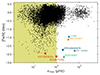 |
Fig. 1. Metallicity [Fe/H] plotted against the frequency of maximum oscillatory power νmax for known oscillating stars, adapted from the left panel of Fig. 2 from Huber et al. (2024). The shaded area represents the region of evolved RGB stars, with a boundary set at νmax ≲ 100 μHz. Noteworthy low-metallicity sub-giant branch (SGB) and RGB stars for which asteroseismic modelling has been performed are highlighted. Note that EPIC206443676 was modelled using the global asteroseismic parameters (Deheuvels et al. 2012), not the individual frequencies as in all other displayed cases. The red stars indicate the two giants considered in the present work. |
The paper is structured as follows: in Sect. 2 we outline the spectroscopic and photometric observations of both stars, before continuing to the asteroseismic observations and reduction in Sect. 3. The details of the grid-based modelling is presented in Sect. 4, with details on the stellar evolution and oscillation codes used. Furthermore, we briefly introduce the BAyesian STellar Algorithm (BASTA; Aguirre Børsen-Koch et al. 2022) used within this work to perform the fitting. Section 5 presents the results obtained for Hennes and Rogue, before discussing their implications and further context in Sect. 6. Lastly, we conclude in Sect. 7.
2. Classical parameters
The various sources for the atmospheric and photometric parameters relevant for the modelling of Hennes and Rogue are outlined in the following. As mentioned in Sect. 1 there are estimations available for both stars from independent determinations. All literature values for the spectroscopic and photometric parameters of interest are listed in Table 1. The nuances and procedures for the estimates originating from this work will be presented below.
Compiled spectroscopic determinations for Hennes and Rogue from various sources.
2.1. Atmospheric observations
The atmospheric analysis was performed on observations taken at the Nordic Optical Telescope (NOT) in 2012/13. Both stars were observed with the FIES spectrograph, which is a fixed-setting spectrograph covering a spectral range of 370−730 nm without gaps (Telting et al. 2014). The observations were carried out with the medium-resolution setting, resulting in a resolving power of R = 46 000. Hennes was observed on a single night in October 2013, obtaining four spectra of an hour each. Rogue was observed on two nights in August 2012, obtaining two spectra of an hour each. Additionally, for Rogue we obtained new high-resolution (R = 67 000) FIES spectra with a combined exposure time of ∼4.8 hours with the NOT in May 2024 in an effort to better characterise the star. The results of this work for Rogue in Table 1 were obtained from these newer spectra.
The spectroscopic analysis followed the method outlined in Slumstrup et al. (2019) by using the asteroseismically determined surface gravity to constrain a classical equivalent width analysis of Fe lines. The effective temperature was varied until excitation equilibrium was reached, that is, no trend being observed between the abundance and the excitation potential of the Fe lines. Likewise, the microturbulence was determined by removing the trend between the abundance and the strength of the Fe lines. Uncertainties were calculated by varying each parameter until at least a 3σ uncertainty was produced on the slope of [Fe/H] vs. excitation potential. Agreement between abundances of FeI and FeII lines to within one standard deviation was assured throughout the analysis. The equivalent widths were measured with DAOSPEC (Stetson & Pancino 2008) and the abundances were calculated with the auxiliary program Abundance with SPECTRUM in LTE (Gray & Corbally 1994). The stellar atmosphere models used are ATLAS9 (Castelli & Kurucz 2004) with solar abundances from Grevesse & Sauval (1998). The stars analysed in the present work are significantly more metal-poor than those of Slumstrup et al. (2019) and therefore it has been necessary to implement NLTE departure-coefficients taken from the INSPECT database version 1.02 (Bergemann et al. 2012; Lind et al. 2012). The alpha enhancement was determined from the Mg abundance with NLTE departure-coefficients.
The metallicities [Fe/H] derived in this work are on average lower than the alternative measurements. However, this is in coherence with expectations as the derived temperatures are also lower. In this parameter space, a lower temperature will provide stronger spectral lines, effectively cancelling out the effect of a lower metallicity. Conversely, in the other estimates the temperatures and metallicities are higher, once again counteracting each other and giving coherent results. The determining factor then becomes the microturbulence as a fitting parameter, which becomes difficult to implement in this very low-metallicity regime for a 1D NLTE approach. The variation seen in [α/Fe] between our results and APOGEE for Rogue likely stems from the different reduction methods, namely equivalent widths and synthetic spectra, respectively. Spectroscopic reduction in the very low-metallicity regime is difficult for both our analysis and the ASPCAP pipeline, as both are optimised for higher metallicities. The comparably higher resolution of the NOT spectra allows for a better determination of the individual spectral line strengths, which is advantageous for this metallicity regime, where so few lines are present.
In the case of Hennes, the choice of spectroscopy required additional considerations. The choice was between our own results from the NOT observations of 2013 and the results of Alencastro Puls et al. (2022) from the HIRES spectrograph (Vogt et al. 1994). The two datasets are consistent within the uncertainties, yet when comparing to purely spectroscopic test-fits to stellar atmospheric models, a self-consistent overlap between all parameters and the models only occur for the HIRES spectroscopy of Alencastro Puls et al. (2022). Furthermore, HIRES is mounted on the larger W. M. Keck telescope and the observations have a higher signal-to-noise ratio than the NOT counterparts for Hennes. We therefore choose to employ the spectroscopic determinations of Alencastro Puls et al. (2022) for the modelling in Sects. 4 and 5. The estimate of the alpha-enhancement [α/Fe] was calculated as the mean of the two alpha-element abundances from magnesium and calcium, with the uncertainty found by adding the individual element uncertainties in quadrature.
For Rogue we chose to use the spectroscopic determination from our present work. They are consistent with the other estimates within the uncertainties. As argued above, the differences seen in Table 1 are likely caused by the difficult parameter space of the star for 1D NLTE approaches, and indicates that both stars would likely benefit from a full 3D NLTE analysis in the future.
2.2. Photometric and astrometric observations
In order to obtain constraints on the stellar luminosities (see Aguirre Børsen-Koch et al. 2022 for details), we need a measure for the parallax and observed magnitudes. In Gaia DR3 (Gaia Collaboration 2016, 2023), the 5-parameter astrometric solution was measured for both Hennes and Rogue as well as the GaiaG, GBP, and GRP magnitudes, hence we can add these to the inference of stellar properties. Hennes has a magnitude of 13.6 in the G band, while Rogue has a magnitude of 11.7. The uncertainties of the Gaia magnitudes are internal and extremely small. A floor of σ = 0.01 was therefore set for all magnitudes retrieved. The Gaia parallaxes were also recovered and have been corrected for their known zero-point error according to the description of Lindegren et al. (2021). This results in a corrected parallax of 0.471 and 0.659 mas for Hennes and Rogue, respectively.
3. Asteroseismic observations and data reduction
Hennes and Rogue were observed in the nominal Kepler mission. The timeseries were recovered from the KASOC database3 after reduction by the pipeline (Handberg & Lund 2014). Subsequently, they were reduced to form the power density spectra (PDS) of both stars following the prescription by Handberg & Campante (2011). Several independent analyses of the PDS were performed, providing primarily the observed individual frequencies for comparison and cross-referencing. Depending on the analysis employed, estimates of the global asteroseismic parameters were also returned. The nuances of the independent determinations and their results are described in Appendix A, where Table A.1 summarises the global asteroseismic parameter estimates obtained. Subsequently, we briefly describe the procedure for obtaining the global asteroseismic parameters in this work.
The value of νmax was found by assuming that the power excess represents a Gaussian envelope (Bedding 2014), where the vertex defines νmax. Repeatedly applying a Gaussian smoothing with a large standard deviation to the PDS allows for the production of the envelope and the subsequent retrieval of νmax for each of the stars. The uncertainty was estimated by varying the length of the timeseries that formed the PDS and changing the width of the Gaussian, meanwhile recording the variations in the derived value for νmax. These estimates agree with those outlined in Appendix A.
For Δν we applied the method of autocorrelation to recover the periodicity stemming from the even spacing in frequency of the p-modes in the PDS. From the autocorrelation function4, the peaks corresponding to multiples of Δν were extracted and a linear correlation through the origin was fitted. The gradient of the linear fit provided Δν with the uncertainty estimated from the associated covariance matrix. Once more, the values of Δν obtained corresponds well with the other independent determinations.
The dipole period spacing ΔΠ1 was determined by employing a de-convolution of the gravity-mode pattern from the mixed-mode pattern (Mosser et al. 2015), which takes into account the signature of a buoyancy glitch (Cunha et al. 2015, 2024; Lindsay et al. 2022). The obtained uncertainty accounts for aliasing effects as described in Appendix A of Vrard et al. (2016). This framework worked for Hennes, and returned a value consistent with the independent determinations. Due to the more evolved nature of Rogue, the proximity between the observed dipole modes exceeds the frequency resolution of the PDS. This, in combination with a weak coupling due to a small coupling factor q (see Sect. 3.2), made the determination of the dipolar period spacing ΔΠ1 very uncertain.
Subsequently, we summarise the obtained parameters for each star and the inferences possible. Thereafter, the observed individual frequencies are presented.
3.1. Hennes – KIC 4671239
Hennes was observed by Kepler from Q1–Q17 in long-cadence mode, with Q6, Q10, and Q14 missing due to the failing of CCD module 3. The resulting timeseries with a length of ∼3.5 years produces the PDS seen in Fig. 2. In this PDS, the dipole mixed modes are clearly separated at higher frequency. This is a result of the unusually high coupling factor of q = 0.26 ± 0.03 found for Hennes, which reflects a small evanescent region in its interior resulting in a strong perturbation to the p-modes by the g-modes (see Sect. 6.3 for a discussion on these aspects). Furthermore, it indicates the less evolved nature of Hennes, where the radiative dampening is not yet strong enough to damp the strongly coupled dipole mixed-modes (Grosjean et al. 2014). We note that one of the independent determinations returned an estimated inclination of 57 ± 2°, which could enforce the possibility of rotational splitting of the modes, tentatively observed for some quadrupole modes in the PDS. Table 2 presents the values obtained for the global asteroseismic parameters of Hennes. The star is thus right past the border to being an evolved RGB star (cf. Fig. 1), confirmed by both the value of Δν and ΔΠ1 (Bedding et al. 2011).
Global asteroseismic parameters for Hennes (KIC 4671239) and Rogue (KIC 7693833).
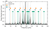 |
Fig. 2. Power density spectrum of Hennes with the consolidated list of individual frequencies from Table A.2 overplotted. Both the raw spectrum (shaded gray) and a Gaussian smoothed version (black) are seen. The orange diamonds, green upwards, and blue downwards triangles depict the ℓ = 0, ℓ = 1, and ℓ = 2 modes, respectively. |
The individual frequencies obtained from all independent determinations for Hennes were manually inspected and compared. The frequencies recovered from the FAMED pipeline (Corsaro et al. 2020) were chosen as they show the most conservative fit to the observed power in the PDS. A cross-match was then performed to only accept frequencies which depicted an overlap within 2σ to the corresponding mode in another set of determinations. The consolidated list of frequencies are displayed in Table A.2 and show 7 detected acoustic orders, with an additional isolated quadrupole mode at low frequency. This consolidated list was later cross-checked by comparing to the results of the TACO code (Hekker et al., in prep.; Themeßl et al. 2020, see Appendix A.4). Figure 2 shows the frequencies overplotted on the PDS, while Fig. 3 displays the modes in an observed power échelle diagram. An échelle diagram uses the even spacing in frequency of the p-modes to stack the PDS vertically in units of Δν. In Fig. 3, the observed power is plotted in a binned grid to allow for visible inspection of the frequency determinations, which should depict a clear overlap with the power. Figure 3 clearly illustrates the evolved mixed-mode pattern of Hennes, where a broad selection of dipole modes have been identified across various mode orders. When using the determined frequencies in Table A.2 for the inference in Sect. 5, we apply a correction to the Doppler-shift stemming from the radial velocity Vr of the star as discussed by Davies et al. (2014). This correction factor is calculated for Hennes to be 1 + Vr/c = 0.99937, where c is the speed of light and Vr is −189.38 km/s obtained from Gaia DR3 data.
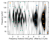 |
Fig. 3. Observed power échelle diagram for Hennes with the consolidated list of individual frequencies from Table A.2 overplotted. The orange diamonds, green upwards, and blue downwards triangles depict the ℓ = 0, ℓ = 1, and ℓ = 2 modes, respectively. An offset has been applied to the x-axis for improved visualisation to avoid wrapping of the radial ridge. |
3.2. Rogue – KIC 7693833
Rogue was observed through Q0–Q17 in long-cadence mode, the entire nominal mission of Kepler, providing a 4-year long timeseries from which the PDS in Fig. 4 is produced. Worth noting is the broadened and substantial power clusters attributed to the dipole modes. In contrast to individual dipole frequency peaks, these clusters arise due to the smaller period spacing and lower coupling strength for this more evolved star, which two independent determinations find to be q ≲ 0.09 (see Table A.1; Dhanpal et al. 2022). The enhances mixing is due to the evolved nature of Rogue, as the oscillation spectrum becomes increasingly dense with evolution (Mosser et al. 2018; Larsen et al. 2024). Furthermore, this results in a slight rightwards shift of the dipole modes from the central position between the ℓ = 0 and ℓ = 2 peaks, as expected from the considerations by Bedding et al. (2010) and Stello et al. (2014).
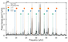 |
Fig. 4. Power density spectrum of Rogue with the consolidated list of individual frequencies from Table A.3 overplotted. Both the raw spectrum and a Gaussian smoothed version are shown as the shaded gray and black spectra, respectively. The orange diamonds, green upwards, and blue downwards triangles depict the ℓ = 0, ℓ = 1, and ℓ = 2 modes, respectively. |
As shown in Table 2, the values of Δν and νmax determined for Rogue indicate an RGB star further evolved compared to Hennes, likely situated just prior to the location of the RGB bump (Khan et al. 2018). The dipole period spacing was determined to be ∼56 ± 2 s. However, as introduced earlier, this determination is very uncertain due to the nature of Rogue. The independent determinations found values ranging from 61 to 105 seconds, with uncertainties as large as 58 seconds. Bearing this in mind, the later modelling of Rogue is unable to consider the period spacing as a global parameter for fitting in Appendix C.
The individual frequencies recovered by the approach of Li et al. (2020) were selected for Rogue, as the determination of the radial (ℓ = 0) and quadrupole (ℓ = 2) modes overlap with all other independent determinations. Furthermore, the frequency set includes only the single p-dominated dipole mode in each mode order. This is desirable, as the reliability of the dipole mixed-mode determination is questionable for Rogue due to the concerns outlined above regarding the frequency resolution and the low coupling factor. The list of determined frequencies is provided in Table A.3 and shows 5 fully detected acoustic orders with two additional isolated modes, one radial and one quadrupole. This consolidated list was also cross-checked against the results of TACO.
The fitting of ℓ = 2 modes as Lorentzian profiles is under the assumption that they originate from a damped oscillator. This may pose issues due to the presence of mixed modes. Mixed modes can lead the fitting process to converge on a specific mixed mode instead of a pure p-mode. This misidentification can result in a smaller line width and an unrealistically low frequency uncertainty. Kjeldsen & Bedding (2012) proposed that frequency uncertainty scales with  , where T is the timeseries duration and τ is the mode lifetime. The mode lifetime τ is related to the linewidth Γ by τ = (πΓ)−1.
In principle, the linewidth of oscillation modes should vary smoothly as a function of frequency (Appourchaux et al. 2014; Lund et al. 2017). Let us consider fitting an ℓ = 2 mode with a linewidth Γ2, and an adjacent ℓ = 0 mode with a linewidth Γ0. If the result shows Γ2 < Γ0, this discrepancy may indicate the fitting issue described earlier. To address this, we inflated the uncertainty of the ℓ = 2 mode frequency by a factor of  .
.
Figure 4 shows the modes overplotted on the PDS, while Fig. 5 indicates the modes in an échelle diagram. As we consider a substantially evolved red giant, a departure in the power distribution from the approximately vertical ridges is seen. Similarly to Hennes, the frequencies displayed in Table A.3 are corrected when input to BASTA. For Rogue, the correction factor is 1 + Vr/c = 0.99998, based on a Vr of −6.86 km/s.
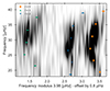 |
Fig. 5. Observed power échelle diagram for Rogue with the consolidated list of individual frequencies from Table A.3 overplotted. The orange diamonds, green upwards, and blue downwards triangles depict the ℓ = 0, ℓ = 1, and ℓ = 2 modes, respectively. An offset has been applied to the x-axis for improved visualisation to avoid wrapping of the radial ridge. |
4. Grid-based modelling of red giants
The modelling of our two red giants followed the grid-based modelling approach. Stellar modelling involves many sources of degeneracy between various input parameters (see Basu & Chaplin 2017 for a review). This poses a challenge for so-called forward modelling, where models are iteratively calculated to match the observations. In this scheme, proper exploration of high-dimensional parameter spaces can become challenging, leading to issues stemming from the unresolved degeneracies. The grid-based method avoids this problem by trading it for a computationally expensive approach through the formation of large-scale grids of stellar models. Traditionally, the grid-based modelling approach was applied to examine suites of numerous stars using the same grid, without the need for recalculating the models. Here, we chose to employ the grid-based modelling for in-depth single-star studies (see e.g. Stokholm et al. 2019; Winther et al. 2023), warranted by the challenging metal-poor and evolved nature of Hennes and Rogue. The production of representative grids for each of the stars in question is costly in terms of computational resources. Yet, it is critical that they contain stellar models that appropriately span the suitable and often wide parameter space, as it provides insight into the degeneracies in and tentative solutions of the modelling.
The stellar evolution models in this work were computed using GARSTEC (Weiss & Schlattl 2008). The equation of state employed in the code originates from the OPAL group (Rogers et al. 1996; Rogers & Nayfonov 2002) and augmented in the low temperature end by that of Mihalas-Hummer-Däppen (Däppen et al. 1988; Hummer & Mihalas 1988; Mihalas et al. 1988, 1990). The treatment of atomic diffusion follows the prescription by Thoul et al. (1994). Various compilations for the opacities are used. For high temperatures it is the ones from OPAL (Rogers & Iglesias 1992; Iglesias & Rogers 1996), while for low temperature the opacities from Ferguson et al. (2005) are used. The nuclear reaction rate cross-sections originate from NACRE (Angulo et al. 1999), except for the reactions 14N(p, γ)15O and 12C(α, γ)16O which are from Formicola et al. (2004) and Hammer et al. (2005), respectively. As both of our stars have low metallicity, there is a possibility of them being α-enhanced, as confirmed by the spectroscopic determinations in Table 1. The stellar abundances used were chosen to be from Asplund et al. (2009), for which versions varying the degree of α-enhancement [α/Fe] in steps of 0.1 dex were calculated and the opacities adjusted. When calculating the synthetic magnitudes of the models, the bolometric corrections by Hidalgo et al. (2018) were used.
4.1. Tailored grids of stellar models
Carrying out detailed grid-based modelling for Hennes and Rogue entailed producing stellar grids for each star. The grids were formed by a local grid-building routine5 which samples the defined parameter space of initial parameters, such as Mini, according to a quasi-random Sobol sampling (Sobol & Levithan 1976; Sobol 1977; Antonov & Saleev 1980; Fox 1986; Bratley & Fox 1988; Joe & Kuo 2003). In setting up these grids, only models on the RGB were included as Hennes and Rogue are in this evolutionary state (see Sects. 1 and 3). However, we also performed initial tests using a wider grid containing tracks evolved through the helium flash and onto the core helium burning phase from Borre et al. (2022). In these tests, we fit the same observables as for the modelling results of Hennes and Rogue presented in Sect. 5, however only the radial mode frequencies were taken into account. The test results confirmed RGB membership, with no likely solutions among post-RGB models. Furthermore, these initial tests provided a rough estimate of the suitable parameter space for each star.
The evolutionary region where models were recorded is defined by an interval in Δν, the value of which decreases with evolutionary stage. The models were evolved from the pre-main sequence until a certain Δν (the lower bounds in Table 3). The evolution in GARSTEC was then halted and diagnostic checks performed, before the calculations were restarted with models being recorded until arriving at the value of Δν indicated by the upper bound in Table 3. An overarching prior on the stellar models is a maximum age of 20 Gyr, for which the calculations were stopped for the given track if reached.
Parameter space of the tailored grids specifying the varied dimensions for Hennes and Rogue.
The boundaries for the spanned parameter space of the tailored grids are listed in Table 3. The parameter space is firstly defined by the stellar mass and metallicity, for which wide boundaries are used that depend on the star in question. For the remaining parameters, the implementation and boundaries used are identical in the two tailored grids. The convective overshooting efficiency fov according to the exponential scheme of Freytag et al. (1996) was varied from zero to modestly above the maximal value fov = 0.016 found through fits to globular clusters (Hjørringgaard et al. 2017). The α-enhancement was sampled from 0 to 0.4 dex. The mixing length parameter αmlt according to the mixing-length description by Kippenhahn et al. (2013) and initial helium abundance Yini were allowed to vary freely (Li et al. 2024). A change in the mixing length can cause differences in Teff of ∼100 K on the RGB (Cassisi 2017; Tayar et al. 2017). It was thus sampled in a wide range from 1.5 to 2.0. Altering Yini will affect the luminosity of the models. Moreover, models with Yini below the Big Bang nucleosynthesis value may sometimes provide a better fit when considering individual frequencies. As such, we allowed for the lower bound to be slightly below this value of YP = 0.24672 ± 0.00017 (Planck Collaboration XIII 2016; Pitrou et al. 2018; Cooke & Fumagalli 2018). This will allow us to check for this tentative situation and add priors subsequently if needed. The effect of mass loss was omitted in the modelling. Both stars are very low-metallicity, low-mass, first-ascent red giants that are situated below the RGB bump, resulting in a low degree of mass loss (Tailo et al. 2020; Tailo 2022). An integration of the mass loss according to the prescription of Reimers (1977), along the best-fitting track found for the most evolved star, Rogue (see Sect. 5.2), finds a cumulated mass loss in the order of 10−5 M⊙, which we found does not impact the modelling.
The tailored grid for Hennes consists of 4096 stellar tracks, while the grid for Rogue is considerably larger consisting of 8192 stellar tracks. The initial test-fitting of Rogue produced a discrepancy between the observed and modelled temperature of the star. Additionally, the overlap with the magnitudes was at times poor. Lastly, Rogue initially indicated a tentative higher mass solution. The combination of these aspects warranted the larger and more exhaustive grid for Rogue.
4.2. Pulsation code and model frequencies
The individual oscillation frequencies for all models in the grids were computed with the Aarhus Adiabatic Pulsation Package (ADIPLS; Christensen-Dalsgaard 2008, version 0.4). Importantly, the extension developed by Larsen et al. (2024) was implemented. This allowed for efficient computation of the individual frequencies in the observable intervals for each model. Previously, the derivation of the individual frequencies for RGB models was only feasible when performing forward-modelling, for which the frequencies could be computed for the few best-fitting models. Here, for the first time in context of grid-based modelling, the mixed modes of both the ℓ = 1, 2 individual frequencies are available for all stellar models before the fitting is performed.
This difference enables us to estimate Δν for the stellar models according to the individual frequencies instead of Eq. (1). Furthermore, it will allow for the fitting of the observed mixed-mode frequencies of Hennes and Rogue to the grids, which is a crucial extension to prior modelling efforts of evolved red giants.
4.3. Fitting observations to models
The fitting algorithm used to match observations to models is the BAyesian STellar Algorithm (BASTA; Aguirre Børsen-Koch et al. 2022). It relies on Bayesian inference to infer a set of model properties given the provided observables. It does so through Bayes’ theorem, which allows for the combination of prior knowledge on the stellar parameters Θ with the data D to yield the likelihood P(D|Θ) of observing the data given the model parameters. For specific details see Aguirre Børsen-Koch et al. (2022). The resulting product from BASTA is a marginalised posterior distribution readily available for inspection. It can be multimodal, meaning it can display more than a single solution for given stellar parameters. As such, is is important to verify the posterior after running the fitting routines. The preferred solution for each parameter is given as the median of the posterior, with uncertainties obtained from the credibility interval formed by the 16th and 84th percentiles of the distribution. Importantly, BASTA is a versatile algorithm that allows for various different observables to be fitted in combination, enabling the detailed modelling that our two stars require.
For clarity, we summarise how the three global asteroseismic parameters are estimated in our modelling. We define νmax according to the asteroseismic scaling relation in Eq. (2). Since we have the individual frequencies available, Δν is determined from weighted differences between the radial frequencies in the given stellar model, following the approach in White et al. (2011). The value of ΔΠ1 is determined from asymptotic expressions for a given model (Mosser et al. 2012, see Aguirre Børsen-Koch et al. 2022 Sect. 4.1.6 for specific details).
4.4. Fitting individual frequencies
The fitting of the individual frequencies follows the default algorithm within BASTA. This consists of two steps for each model. Firstly, given the abundance of mixed modes in the models, the matching of observed modes to modes in the model is performed. This is done using the standard method in BASTA (see Sect. 3.1 of Ball et al. 2020; Aguirre Børsen-Koch et al. 2022; Stokholm et al., in prep.), with subtle adjustments for application to red-giant stars (a summary of the algorithm can be found in Appendix E). Secondly, after identifying the matching ℓ = 0, 1, 2 model frequencies, they are corrected using the surface correction of Ball & Gizon (2014) using only the cubic term. We choose to use only the cubic term as we fit a modest number of modes for Rogue, which means we are unable to properly constrain the inverse term of Ball & Gizon (2014) and risk overfitting. We note, however, that the posteriors remain unchanged when using the complete formulation.
There exist previous studies on the application of this surface correction on the RGB, which mention an over-correction issue due to the inertia scaling (Li et al. 2018; Ball et al. 2018). The application of the surface correction may result in the non-radial mixed modes being out of order, that is, the monotonic relationship between mode order and frequency of the theoretical frequencies is broken. This is because the surface correction shifts an acoustic resonance beyond the adjacent oscillations due to its comparably lower inertia. Matching the observed mixed modes to the surface corrected frequencies would thus mean potentially matching to an unphysical representation of the oscillation spectrum. We avoid this as the matching in BASTA is performed before application of the surface correction. Subsequently, when the surface correction is applied, we find that the effect described in Ball et al. (2018) impacts the models in the grid for Rogue. Yet, due to the order of the matching procedure, it will not change the statistics of the performed fitting. A discussion regarding the performance of the frequency matching algorithm can be found in Sect. 6.1.
5. Results of asteroseismic modelling
The modelling of Hennes and Rogue was extensively explored and included a variety of different fitting cases and consistency tests. In the following, for the sake of brevity and clarity, we present only the case that represents the key extension to prior efforts that this work contributes: the fitting of the individual frequencies. As will become clear, this case is the only approach that yields self-consistent results and provide proper overlap between the constraints from the observables. We thus fit the individual frequencies for Hennes and Rogue in Tables A.2 and A.3, respectively. In addition the fits included the observed spectroscopic parameters Teff, [Fe/H], and [α/Fe] along with the distance through the combination of parallax with the GaiaG, BP, and RP magnitudes.
5.1. Hennes – KIC 4671239
The results for Hennes are displayed in Table 4, compared with the results of Alencastro Puls et al. (2022). For inspection of the posteriors, see Fig. B.1. The detailed asteroseismic modelling with tailored grids and individual frequencies in this work has solved the tension of prior results displaying a low stellar age (presented in Sect. 1). Hennes being a metal-poor halo star (see Sect. 6.4) is now classified as a low-mass high-age star, in coherence with expectations.
Modelling results for Hennes.
Figure 6 shows the fit of the individual frequencies in a replicated échelle diagram. The fit to the individual frequencies is satisfactory and shows a best-fitting model with a mixed mode pattern matching that of Hennes very closely. Fitting the dipole mixed-modes directly allows us to capture the underlying period spacing of the model, clearly seen in the most populated mode orders in Fig. 6. The resulting prediction of ΔΠ1 from the fit is also consistent with the observed value. The modelled Δν value is in accordance with the observed. We note that the three lowest radial modes in the figure deviate from the model due to significant curvature of the observed ridge (Mosser et al. 2013). Furthermore, as the cubic surface correction of Ball & Gizon (2014) is scaled with mode inertia, the radial modes are shifted further than the quadrupoles for a given surface correction coefficient. This results in a erroneous appearance of the small spacing δν02 in the surface-corrected model in Fig. 6, but does not reflect the small spacing in the model. Notably, the predicted νmax value from the fit deviates significantly from the observed. This discrepancy is discussed in detail in Sect. 6.2.
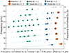 |
Fig. 6. Échelle diagram of Hennes with the fitted individual frequencies matched to the modes of the best-fitting model. The orange diamonds, green upwards, and blue downwards triangles depict the ℓ = 0, ℓ = 1, and ℓ = 2 modes, respectively. The cubic term of the surface correction by Ball & Gizon (2014) has been applied to the model frequencies, with a surface correction coefficient of a3 = −7.0512 ⋅ 10−8. The size of the model modes is scaled related to the inverse of their respective inertia. An offset has been applied to the x-axis for improved visualisation to avoid wrapping of the radial ridge. |
Figure 7 illustrates the result in a Kiel diagram (a spectroscopic HR diagram) plotting the surface gravity log(g) against effective temperature. Only the tracks containing statistically significant models are plotted, forming the dense distribution of stellar tracks seen. The observational constraints for the fitted parameters are overlaid onto the plot for a representative region along each track depicting the 1-σ uncertainty (Hjørringgaard et al. 2017). Notably, the frequency constraint band is formed based on a selection of models matching the radial frequencies, not taking into account the non-radial oscillations in the spectrum. The results display a satisfactory overlap between all observational constraints. Importantly, this kind of overlap remained unattainable in the prior efforts when fitting the global asteroseismic parameters and, crucially, persists in this work if we perform the same fitting approach (see Appendix C). Hence, a proper inference for Hennes is only attainable when utilising the individual mode frequencies to avoid the dependence on the asteroseismic scaling relations, as has been presented here.
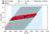 |
Fig. 7. Kiel diagram of Hennes displaying a representative number of stellar tracks in the grid. The observed constraints on the fitted parameters are overlaid to show an overlap with the median and best-fitting model from the posterior. |
5.2. Rogue – KIC 7693833
The results obtained for Rogue are displayed in Table 5, where the results of Pinsonneault et al. (2025) are also included. For inspection of the posteriors, see Fig. B.2. The obtained parameters in this work indicate a low-mass star with an accordingly high age. These results are in tension with those obtained in prior efforts and with Pinsonneault et al. (2025), yet now comply with the expectations for a low-metallicity star.
Modelling results for Rogue.
Figure 8 displays the fit to the individual frequencies for Rogue. The more evolved nature of the best-fitting model is immediately apparent from the denser theoretical frequency spacing for each acoustic mode order. The fit to the individual frequencies is satisfying, however with some artefacts of the frequency matching algorithm impacting the quadrupole modes. This will be further discussed in Sect. 6.1. The modelled Δν value is slightly higher than the observed. This is due to the Δν value in the grid being estimated from a weighted average between the non-surface-corrected radial frequencies. Hence, the obtained value will be somewhat higher, but by inspection of Fig. 8 is suitable for creating the vertical ridge structure in the échelle diagram. It may be noted that the modelled period spacing of  s is roughly in accordance with the uncertain observational estimate of ΔΠ1 = 56.6 s discussed in Sect. 3.2. The νmax discrepancy found for Hennes is also clear for Rogue.
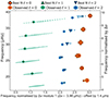 |
Fig. 8. Échelle diagram of Rogue with the fitted individual frequencies matched to the modes of the best-fitting model. The orange diamonds, green upwards, and blue downwards triangles depict the ℓ = 0, ℓ = 1, and ℓ = 2 modes, respectively. The cubic term of the surface correction by Ball & Gizon (2014) has been applied to the model modes, with a surface correction coefficient of a3 = −1.5554 ⋅ 10−7. The size of the model modes is scaled related to the inverse of their respective inertia. An offset has been applied to the x-axis for improved visualisation to avoid wrapping of the radial ridge. |
Figure 9 illustrates the result in a Kiel diagram, similar to that made for Hennes. At first glance, it appears counter-intuitive why the best-fitting model and median posterior solutions do not lie at lower temperatures where the frequency constraints overlap perfectly with the Gaia magnitudes. This is because the frequency constraint band is formed based on the radial frequencies only, allowing the best-fitting model and median solutions, which take into account the complete mode spectrum and other fit parameters, to lie away from the visual overlap. A clear ∼2.3σ deviation from the observed temperature is found, an unresolved complication present for Rogue. Crucially, the best-fitting model and seismic solution is consistent with all other observables, and provide a modelling result, which is not in tension with prior expectations from the low-metallicity nature of the star. In Sect. 6.1 we discuss the nuances of the modelling challenges for Rogue, where a more thorough evaluation will be presented.
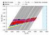 |
Fig. 9. Kiel diagram of Rogue displaying a representative number of stellar tracks in the grid. The observed constraints on the fitted parameters are overlaid to show an overlap with the median and best-fitting model from the posterior. A clear discrepancy between the observed and modelled temperature is found, with the lower 1-σ uncertainty visualised by the boundary of the blue region. |
6. Asteroseismic characterisation from individual frequency modelling
This work has demonstrated that rigorous asteroseismic modelling is feasible for evolved red giants, even in the most challenging cases of the very low-metallicity regime. We emphasize that the results obtained are not reproduced if one considers the global asteroseismic parameters in the fitting (see Appendix C). This suggests that future studies of red giants could benefit from relying more on the individual frequencies as direct observable constraints in the modelling.
Hennes is the first metal-poor star with νmax below 100 μHz to be asteroseismically modelled with ℓ = 0, 1, 2 mixed-mode individual frequencies within a grid-based methodology. Importantly, at this stage of evolution, we can clearly observe several dipole mixed modes within each acoustic mode order. As shown in Fig. 6, this allows us to capture the underlying period spacing during the modelling, effectively providing constraints on the interior stellar structure. Rogue further extends the coverage of metal-poor stars with asteroseismic individual frequency modelling to the region where νmax is below 35 μHz. Here, the mixed mode pattern has become so dense and the period spacing so low that we cannot confidently resolve the dipole mixed modes observationally. Additionally, the inertia of the g-dominated modes increases, making their detection difficult. Only the observational estimate for the acoustic resonances of each mode order were fitted, however to models containing all potentially observable mixed modes, which allows for the opportunity of matching several theoretical frequencies. This allowed for the classification of a particularly vexing star, however, a significant temperature discrepancy between the observed and modelled values persists.
6.1. Modelling nuances of Rogue
In Fig. 9 a clear discrepancy between the observed and modelled temperature was seen. A likely cause was mentioned in Sect. 2.1, namely the application of 1D NLTE spectroscopic reduction methods for the very low-metallicity regime. The degeneracy between the temperature and metallicity, as well as the implementation of the microturbulence as a fitting parameter, may very well lead to inconsistencies on the observational side. Furthermore, the temperature of the RGB stellar models is also a topic of discussion. Cassisi (2017) showed how the temperature of RGB models is sensitive to αMLT and the outer boundary condition employed in the T(τ) relation for the choice of atmosphere. These aspects were further outlined by Tayar et al. (2017), who presented a metallicity dependent temperature offset for RGB stars when compared to theoretical predictions, suggesting to make the convective mixing length metallicity dependent to account for the effect. Salaris et al. (2018) later reanalysed the sample from Tayar et al. (2017), and found that the discrepancy was only significant for α-enhanced RGB stars. Schonhut-Stasik et al. (2024) also argued that the choice of temperature scales for low-metallicity red-giant models may lead to discrepancies. It is noteworthy that this temperature discrepancy was not present for Hennes while being so prominent for Rogue. A planned future study employing a larger sample of low-metallicity giants will likely aid in classifying the occurrence and behavioural trends of the temperature discrepancy.
In the frequency fit of Rogue in Fig. 8, certain quadrupole modes appear to be mismatched, for example in the highest mode order. The frequency matching algorithm in BASTA was developed for main-sequence and sub-giant stars (see e.g. Stokholm et al. 2019). For the former, only one mode exists per acoustic mode order and for the latter there is a large difference in mode inertia between the few modes in each mode order. On the RGB and with the oscillation spectra obtained through the application of the truncated scanning method of Larsen et al. (2024), we obtain a modest number of mixed modes closely spaced in frequency and of comparable inertia within each mode order. This means that the matching algorithm described briefly in Sect. 4.4 may not be entirely suitable for application to red giants. However, we stress that forcing the solution to the ‘by-eye’ optimal solution for the best-fitting model in Fig. 8 has no impact on the choice of optimal model during the fitting. A test was carried out simply matching the observed mode of each degree to the respective model frequency with the lowest inertia within each acoustic mode order. This does not significantly change the drawn posteriors, as the contribution to the likelihood from the above change is less significant than the evolution of particularly the radial frequency spectrum between consecutive models. A proper evaluation of a refined RGB mixed-mode frequency matching algorithm requires statistics on the performance based on more than the two stars at hand, which is the subject of a future study.
6.2. Circumventing the νmax scaling relation dependence
The estimates for νmax obtained from the modelling posteriors showed a significant discrepancy to the observed for both stars. To reiterate, the νmax value of the models are predicted using the scaling relation in Eq. (2) as no other alternative exists. We circumvented the dependence on the scaling relations entirely by fitting the individual frequencies, resulting in the highest-likelihood models being selected based on the direct constraints that the frequencies provide to the interior model structures. This difference suggests a metallicity dependence on the νmax scaling relation, which becomes significant for very low-metallicity stars. This agrees with the dependence of νmax on the Mach number found by Belkacem et al. (2011) and with other previous studies finding the same indication, albeit in different metallicity or evolutionary regimes (Epstein et al. 2014; Li et al. 2022, 2024; Campante et al. 2023).
Investigating this metallicity dependence means evaluating a correction factor to the scaling relation,
 (3)
(3)
 (4)
(4)
Here, νmax, BFM can be extracted from the best-fitting model of Hennes and Rogue while νmax, obs are the observed values shown in Table 2. The values are νmax, BFM = 89.83 and νmax, BFM = 29.60 μHz, resulting in correction factors of fνmax = 1.101 and fνmax = 1.098, for Hennes and Rogue, respectively. This yields a difference in νmax of ∼10%, showing that the uncorrected νmax scaling relation in the metal-poor regime is significantly less accurate than near solar metallicities. We can express this difference in mass using the observed νmax, Δν, and Teff to calculate the scaling relation estimate as,
 (5)
(5)
 (6)
(6)
Using the scaling relation in Eq. (5), this results in a ∼30% and ∼40% larger mass from the scaling relation than from the determination when performing asteroseismic individual frequency modelling. This seconds the findings of Huber et al. (2024) who similarly recovered a ∼24% difference in mass for KIC 8144907 with [Fe/H]= − 2.66 dex. The tension remains when using proposed Δν metallicity corrections (Viani et al. 2017) and repeating the above exercise. For these three RGB stars with individual frequency modelling, the situation thus hints towards an increasing discrepancy with evolution for these similarly very metal-poor giants.
Lastly, we note that for the stars KIC 7341231 (Deheuvels et al. 2012), ν Indi (Chaplin et al. 2020), and HD 140283 (Lundkvist et al., in prep.) with individual frequency modelling shown overplotted in Fig. 1, the tentative metallicity dependence on νmax between observed and model values was also seen.
6.3. Enhanced mode mixing at low metallicity
During this work concerning stellar modelling of low-metallicity giants, a property of the interior profiles in the models was noticed. The extent of the evanescent region was increased and the coupling weakened with increasing metallicity. Here, we wish to briefly clarify and present this trend seen in the models.
Figure 10 depicts a propagation diagram of three stellar models, showing the proximity of the oscillation cavities in the deep interior of the models. The very low-metallicity model is the best-fitting model of Hennes. The other two were calculated with identical initial parameters and varying the metallicity to [Fe/H]= − 1.3 and [Fe/H] = 0.0. The buoyancy frequency N (Tassoul 1980) and Lamb frequency Sℓ (Lamb 1932) are calculated using Eqs. (2) and (3) of Larsen et al. (2024), respectively. The figure shows that the depth of the convective zone increases with increasing metallicity, as a result of the dependence of convection on the opacity and thus chemical composition. This effectively increases the extent of the evanescent region (as shown by the shaded bands of each model) for a representative frequency here chosen as the observed νmax of Hennes. Equations (11) and (12) of Hekker & Christensen-Dalsgaard (2017) allows us to evaluate the dipole period spacing and Eq. (9) of Larsen et al. (2024) provides an estimate of the coupling constant. The obtained values, overplotted on Fig. 10, clearly illustrate the same trend: a decreasing period spacing and increasing coupling constant with decreasing metallicity.
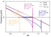 |
Fig. 10. Propagation diagram for three stellar models depicting the characteristic frequencies in the interior near the lower convective boundary. The best-fitting model of Hennes is plotted alongside two models of similar evolutionary state, i.e. similar Δν value, with identical initial parameters except for a variation in [Fe/H]. The shaded region around the observed νmax of Hennes represents the extent of the evanescent region for the three models, which increases with metallicity. |
This effect should lead to a stronger mixing between the p- and g-modes of low-metallicity stars, resulting in a larger frequency displacement for the mixed modes within a given acoustic order. Additionally, the difference in the period spacing and coupling constant will affect Eq. (28) of Mosser et al. (2018), which describes the frequency range in which mixed modes should be observable around an acoustic resonance, hinting towards a possible metallicity dependence. Confirming the postulated property of mixed-mode behaviour as a function of metallicity would require a dedicated study of the trend in observed oscillation spectra of RGB stars, which is beyond the scope of this work.
6.4. Galactic context
The Galactic orbital characteristics of the stars were determined from the 5D astrometric information and line-of-sight velocities from Gaia DR3 (Gaia Collaboration 2016, 2023). We used the PYTHON package galpy (Bovy 2015) for this computation of the Galactic orbital properties. As a description of the Milky Way potential, we used the axisymmetric gravitational potential McMillan2017 (McMillan 2017). As for the Galactic location and velocity of the Sun, we assumed (X⊙, Y⊙, Z⊙) = (8.2, 0, 0.0208) kpc and  with a circular velocity of 240 km s−1 (Schönrich et al. 2010; Bennett & Bovy 2019; GRAVITY Collaboration 2019).
We used the implementation of the action-angle estimation algorithm ‘Stäckel fudge’ (Binney 2012) in galpy with a focal length focus of 0.45 to calculate orbit information such as actions, eccentricity, and maximum orbit Galactocentric height. By leveraging the uncertainties and correlations in the astrometric measurements to create a multivariate normal distribution, we performed 10 000 iterations to generate distributions of the orbital properties. The 16th, 50th, and 84th percentiles of these distributions were then used as numerical estimates of the orbital values and their associated uncertainties. The complete list of orbital properties for Hennes and Rogue can be found in Table D.1 in the Appendix.
Fig. 11 illustrates the integrated orbits of Hennes and Rogue within the Milky Way’s gravitational potential, highlighting their differing extents. Hennes traverses the dense inner regions of the Galaxy, with an inner turning point nearly 1 kpc from the Galactic centre. Additionally, Hennes frequently moves far from the Galactic disk, reaching heights several kiloparsecs above the Galactic midplane. In contrast, while Rogue does venture beyond the Local Solar Neighbourhood, its orbit more closely resembles that of the Sun, differing significantly from the more extensive and dynamic path of Hennes.
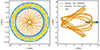 |
Fig. 11. Integrated orbit of Rogue and Hennes within the Milky Way’s potential over a 10 Gyr period, depicted in Cartesian Galactocentric coordinates. The left panel presents a top-down view of the Galaxy (x, y), while the right panel shows an edge-on perspective (x, z). The Sun’s integrated orbit is included in both views as a reference. |
Fig. 12 shows the location of the stars in a Toomre diagram, in which the horizontal axis depicts motion around in the plane and the vertical axis represents motion perpendicular to the horizontal axis. This representation helps distinguish different Galactic components more clearly. In this context, Hennes stands out as behaving like a typical halo star, characterized by its lower rotational velocity within the Galactic plane and higher velocities in the vertical (up-down) and radial (in-out) directions compared to the Sun. Rogue is more intriguing, as it appears to align with the characteristics of a thin disk star, exhibiting only slightly higher velocities in the direction perpendicular to the Galactic plane.
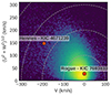 |
Fig. 12. Toomre diagram showing the Galactic velocity components. The vertical axis represents motion perpendicular to the plane and the horizontal axis depicts motion within the plane. The location of Hennes and Rogue in this space are marked with red dots. The background density map represents the number count of single targets from Gaia DR3 with reliable astrometric data and available line-of-sight velocities (astrometric_params_solved = 95, non_single_star = 0, ruwe < 1.4, and rv_nb_transits > 0). |
6.5. Possible Galactic origins
In this section, we assess the possible Galactic origins of the two stars based on their combined kinematics, spectroscopic, and age signatures. Kinematically Hennes looks like a characteristic halo star. It has a low orbital energy and the orbit looks kinematically heated in velocities, eccentricity, and angular momentum. The position of Hennes in angular momenta-orbital energy dimensions could place it in either L-RL3 (Ruiz-Lara et al. 2022; Dodd et al. 2023), Heracles (Horta et al. 2021), or in a metal-poor tail of Gaia-Enceladus (Helmi et al. 2018). In either of these cases, Hennes would be the most metal-poor member of each association discovered to date.
The orbit of Rogue is similar to those of the older members of the Galactic thin disk, which is peculiar given its age and metallicity. This suggests that Rogue is part of this controversial, ancient, and very metal-poor stellar population in the Milky Way. The discovery of very metal-poor stars exhibiting disc-like kinematics and a preference for prograde over retrograde orbits has recently generated significant interest within the community (Sestito et al. 2019; Cordoni et al. 2021; Belokurov & Kravtsov 2022; Carollo et al. 2023; Bellazzini et al. 2024; Ardern-Arentsen et al. 2024; Fernández-Alvar et al. 2024). Studies of these metal-poor stars with prograde planar orbits can provide us insights into the earliest phase of the formation of the Milky Way discs and there is still many unanswered questions. From simulations of model galaxies, Sotillo-Ramos et al. (2023) found that the fraction of very metal-poor stars in the kinematically cold disc component varies from 5 − 10% up to 40%, with typical values around 20% and an occurrence rate that seem to decrease with decreasing metallicity. Other comparisons with simulations of Milky Way analogues suggests that most stars in this population likely originated from accretion events on nearly planar orbits (Sestito et al. 2021) as the emergence of this population is unlikely to be induced by a rotating galactic bar (Yuan et al. 2024). Nepal et al. (2024) emphasized that many disc galaxies at high redshifts possess an ancient and kinematically cold disc formed in situ, suggesting that this metal-poor population could represent our Galaxy’s analogue.
If Rogue is representative of the population, then we can use its stellar age as a constraint when assessing the possible origins. Given Rogue’s characteristics, the detailed modelling of Rogue using asteroseismic constraints is more aligned with the view that this population originates from multiple accretion events, in which the accretion occurred close to planar orbits, than with the view that this stellar population can solely be a single, unperturbed ancient metal-poor thin disk. As it is possible that multiple channels contribute to the formation of this population, with Rogue belonging to one and not the other, a future study employing asteroseismology for this population of stars appears to be the next step.
7. Conclusion
This work proves that asteroseismic individual frequency modelling is possible within the grid-based modelling scheme for evolved red giants. Proper determination of global stellar properties in the very metal-poor regime has been shown to crucially depend on how the stellar inference is made. The main conclusions of this paper are as follows:
-
The two very low-metallicity stars, KIC 4671239 and KIC 7693833, have been characterised with stellar properties that are coherent with expectations from Galactic archaeology. Hennes and Rogue were found to have masses of
 and
and  with an age of
  and
and  Gyr, respectively. Both stars had for a long time defied such characterisation, as they are situated in a very difficult region of parameter space for stellar modelling, yet individual frequency modelling in combination with detailed grid-based approaches has made it possible. Crucially, the obtained self-consistency could not be obtained when fitting the global asteroseismic parameters in the past nor in the contemporary work. This fact speaks to the benefits of future application of individual frequency modelling for giants.
 -
A metallicity dependence of the asteroseismic scaling relation for νmax was seen through a clear discrepancy between the observed and modelled values for Hennes and Rogue of ∼10%, with the νmax predicted from the asteroseismic scaling relation being too small compared to the observations. In the determination of global stellar properties for very metal-poor stars in general, such a difference would correspond to overestimations in mass by ∼30%, leading to wrongful conclusions about the age demographics of the population. This result is consistent with prior findings by for example Belkacem et al. (2011), Li et al. (2022), and Huber et al. (2024). Yet, it is also in slight tension with studies by Zhou et al. (2024), finding that for the case of main sequence stars νmax shows no metallicity dependence. However, the conclusion of Zhou et al. (2024) may not hold in the case of more evolved stars in the sub-giant or red-giant branch phases of their lives. To answer this question definitively will require further studies on both the theoretical and observational side, something which is currently in progress.
-
Accurate and precise stellar ages are crucial for unravelling the timeline of events in the Galaxy. The impact of the systematic effect of metallicity on the νmax scaling relation can be significant for Galactic archaeology as asteroseismic targets are typically used as calibrators. In recent years, stellar remnants of galaxies that merged with the early Milky Way have been a particular topic of interest for the community (see e.g. Helmi 2020, for a review). We have identified Hennes to be a member of one of such halo populations, making it the most metal-poor member with detailed modelling using asteroseismic constraints. Rogue seems to be a member of the ancient very metal-poor population with prograde, planar orbits – providing a valuable age constraint to studies of the earliest phase of the formation of the Milky Way disc structures.
We emphasise the possibilities of circumventing the dependence on the asteroseismic scaling relations and directly fitting the individual frequencies of red giants. Observationally, Kepler and the work by observational astronomers has supplied us with high-quality detection of the individual frequencies of giants, which is continuously being expanded by missions such as the Transiting Exoplanet Survey Satellite (TESS; Ricker et al. 2014) and in the future the PLAnetary Transits and Oscillations of stars mission (PLATO; Rauer et al. 2024). It is now possible following the work by Larsen et al. (2024) to utilise the individual frequencies to their full potential and this paper has demonstrated that it works in one of the most challenging regions for stellar modelling. We therefore suggest that such efforts should be pursued in the future as it may allow for refinement of our understanding of stars on the RGB. For example, investigations resolving the convective zone boundaries probed by the period spacing ΔΠ1 could be further developed by the inclusion of the mixed-mode dipole individual frequencies, which directly probes this region in the stellar interior through their sensitivity to the mode coupling (Jiang & Christensen-Dalsgaard 2014; Pinçon et al. 2019). These efforts in turn link to the study of the origin behind magnetic fields in red giant stars (see e.g. Deheuvels et al. 2023; Das et al. 2024); a field of research that is still in its infancy.
Data availability
All data and stellar grid products are available upon reasonable request to the first author.
The literature values that form the black points in the plot are from Pinsonneault et al. (2014), Serenelli et al. (2017), Matsuno et al. (2021), and Schonhut-Stasik et al. (2024).
Available at www.inspect-stars.com
Calculated with the STATSMODELS module ACF https://www.statsmodels.org/stable/generated/statsmodels.tsa.stattools.acf.html
Named AUbuild; planned for eventual public release.
The public GitHub repository is available at https://github.com/EnricoCorsaro/DIAMONDS
Available at https://github.com/OthmanB/TAMCMC-C
Acknowledgments
We thank the anonymous referee for the detailed and constructive feedback on the manuscript. JRL wishes to thank the members of SAC and the collaborators of the prior efforts for valuable comments and discussions regarding the paper. Furthermore, we appreciate being given access to the data for and the allowed inclusion of Fig. 1 by Daniel Huber. This work was supported by a research grant (42101) from VILLUM FONDEN. Funding for the Stellar Astrophysics Centre was provided by The Danish National Research Foundation (grant agreement no.: DNRF106). MSL acknowledges support from The Independent Research Fund Denmark’s Inge Lehmann program (grant agreement no.: 1131-00014B). The numerical results presented in this work were obtained at the Centre for Scientific Computing, Aarhus https://phys.au.dk/forskning/faciliteter/cscaa/. AS acknowledges support from the European Research Council Consolidator Grant funding scheme (project ASTEROCHRONOMETRY, G.A. n. 772293, http://www.asterochronometry.eu). This work presents results from the European Space Agency (ESA) space mission Gaia. Gaia data are being processed by the Gaia Data Processing and Analysis Consortium (DPAC). Funding for the DPAC is provided by national institutions, in particular the institutions participating in the Gaia MultiLateral Agreement (MLA). The Gaia mission website is https://www.cosmos.esa.int/gaia. The Gaia archive website is https://archives.esac.esa.int/gaia. This paper includes data collected by the Kepler mission and obtained from the MAST data archive at the Space Telescope Science Institute (STScI). Funding for the Kepler mission is provided by the NASA Science Mission Directorate. STScI is operated by the Association of Universities for Research in Astronomy, Inc., under NASA contract NAS 5-26555. SH acknowledges support from the European Research Council under the European Community’s Horizon 2020 Framework/ERC grant agreement no 101000296 (DipolarSounds). D.S. is supported by the Australian Research Council (DP190100666).
References
- Abdurro’uf, Accetta, K., Aerts, C., et al. 2022, ApJS, 259, 35 [NASA ADS] [CrossRef] [Google Scholar]
- Aguirre Børsen-Koch, V., Rørsted, J. L., Justesen, A. B., et al. 2022, MNRAS, 509, 4344 [Google Scholar]
- Alencastro Puls, A., Casagrande, L., Monty, S., et al. 2022, MNRAS, 510, 1733 [Google Scholar]
- Anderson, E. R., Duvall, T. L., & Jefferies, S. M. 1990, ApJ, 364, 699 [NASA ADS] [CrossRef] [Google Scholar]
- Angulo, C., Arnould, M., Rayet, M., et al. 1999, Nucl. Phys. A, 656, 3 [Google Scholar]
- Antonov, I., & Saleev, V. 1980, USSR Comput. Math. Math. Phys., 19, 252 [Google Scholar]
- Appourchaux, T., Antia, H. M., Benomar, O., et al. 2014, A&A, 566, A20 [NASA ADS] [CrossRef] [EDP Sciences] [Google Scholar]
- Ardern-Arentsen, A., Monari, G., Queiroz, A. B. A., et al. 2024, MNRAS, 530, 3391 [NASA ADS] [CrossRef] [Google Scholar]
- Asplund, M., Grevesse, N., Sauval, A. J., & Scott, P. 2009, ARA&A, 47, 481 [NASA ADS] [CrossRef] [Google Scholar]
- Ball, W. H., & Gizon, L. 2014, A&A, 568, A123 [NASA ADS] [CrossRef] [EDP Sciences] [Google Scholar]
- Ball, W. H., Themeßl, N., & Hekker, S. 2018, MNRAS, 478, 4697 [Google Scholar]
- Ball, W. H., Chaplin, W. J., Nielsen, M. B., et al. 2020, MNRAS, 499, 6084 [NASA ADS] [CrossRef] [Google Scholar]
- Balser, D. S. 2006, AJ, 132, 2326 [Google Scholar]
- Basu, S., & Chaplin, W. J. 2017, Asteroseismic Data Analysis: Foundations and Techniques (Princeton: Princeton University Press) [Google Scholar]
- Bedding, T. R. 2014, Asteroseismology (Cambridge: Cambridge University Press) [Google Scholar]
- Bedding, T. R., Huber, D., Stello, D., et al. 2010, ApJ, 713, L176 [Google Scholar]
- Bedding, T. R., Mosser, B., Huber, D., et al. 2011, Nature, 471, 608 [Google Scholar]
- Belkacem, K., Goupil, M. J., Dupret, M. A., et al. 2011, A&A, 530, A142 [CrossRef] [EDP Sciences] [Google Scholar]
- Bellazzini, M., Massari, D., Ceccarelli, E., et al. 2024, A&A, 683, A136 [NASA ADS] [CrossRef] [EDP Sciences] [Google Scholar]
- Belokurov, V., & Kravtsov, A. 2022, MNRAS, 514, 689 [NASA ADS] [CrossRef] [Google Scholar]
- Bennett, M., & Bovy, J. 2019, MNRAS, 482, 1417 [NASA ADS] [CrossRef] [Google Scholar]
- Benomar, O., Appourchaux, T., & Baudin, F. 2009, A&A, 506, 15 [NASA ADS] [CrossRef] [EDP Sciences] [Google Scholar]
- Benomar, O., Bedding, T. R., Mosser, B., et al. 2013, ApJ, 767, 158 [Google Scholar]
- Benomar, O., Belkacem, K., Bedding, T. R., et al. 2014, ApJ, 781, L29 [Google Scholar]
- Bergemann, M., Lind, K., Collet, R., Magic, Z., & Asplund, M. 2012, MNRAS, 427, 27 [Google Scholar]
- Binney, J. 2012, MNRAS, 426, 1324 [Google Scholar]
- Borre, C. C., Aguirre Børsen-Koch, V., Helmi, A., et al. 2022, MNRAS, 514, 2527 [NASA ADS] [CrossRef] [Google Scholar]
- Borucki, W. J., Koch, D., Basri, G., et al. 2010, Science, 327, 977 [Google Scholar]
- Bovy, J. 2015, ApJS, 216, 29 [NASA ADS] [CrossRef] [Google Scholar]
- Bratley, P., & Fox, B. 1988, ACM Trans. Math. Softw., 14, 88 [Google Scholar]
- Brogaard, K., VandenBerg, D. A., Bruntt, H., et al. 2012, A&A, 543, A106 [NASA ADS] [CrossRef] [EDP Sciences] [Google Scholar]
- Brogaard, K., Arentoft, T., Slumstrup, D., et al. 2022, A&A, 668, A82 [NASA ADS] [CrossRef] [EDP Sciences] [Google Scholar]
- Brown, T. M., Gilliland, R. L., Noyes, R. W., & Ramsey, L. W. 1991, ApJ, 368, 599 [Google Scholar]
- Campante, T. L., Li, T., Ong, J. M. J., et al. 2023, AJ, 165, 214 [NASA ADS] [CrossRef] [Google Scholar]
- Carollo, D., Christlieb, N., Tissera, P. B., & Sillero, E. 2023, ApJ, 946, 99 [NASA ADS] [CrossRef] [Google Scholar]
- Casagrande, L., Silva Aguirre, V., Stello, D., et al. 2014, ApJ, 787, 110 [CrossRef] [Google Scholar]
- Cassisi, S. 2017, Eur. Phys. J. Web Conf., 160, 04002 [Google Scholar]
- Castelli, F., & Kurucz, R. L. 2004, ArXiv e-prints [arXiv:astro-ph/0405087] [Google Scholar]
- Chaplin, W. J., & Miglio, A. 2013, ARA&A, 51, 353 [Google Scholar]
- Chaplin, W. J., Serenelli, A. M., Miglio, A., et al. 2020, Nat. Astron., 4, 382 [Google Scholar]
- Christensen-Dalsgaard, J. 2008, Ap&SS, 316, 113 [Google Scholar]
- Christensen-Dalsgaard, J., Dappen, W., Lebreton, Y. 1988, Nature, 336, 634 [Google Scholar]
- Cooke, R. J., & Fumagalli, M. 2018, Nat. Astron., 2, 957 [Google Scholar]
- Cordoni, G., Da Costa, G. S., Yong, D., et al. 2021, MNRAS, 503, 2539 [NASA ADS] [CrossRef] [Google Scholar]
- Corsaro, E. 2019, Front. Astron. Space Sci., 6, 21 [Google Scholar]
- Corsaro, E., & De Ridder, J. 2014, A&A, 571, A71 [NASA ADS] [CrossRef] [EDP Sciences] [Google Scholar]
- Corsaro, E., Mathur, S., García, R. A., et al. 2017, A&A, 605, A3 [NASA ADS] [CrossRef] [EDP Sciences] [Google Scholar]
- Corsaro, E., McKeever, J. M., & Kuszlewicz, J. S. 2020, A&A, 640, A130 [NASA ADS] [CrossRef] [EDP Sciences] [Google Scholar]
- Cunha, M. S., Stello, D., Avelino, P. P., Christensen-Dalsgaard, J., & Townsend, R. H. D. 2015, ApJ, 805, 127 [NASA ADS] [CrossRef] [Google Scholar]
- Cunha, M. S., Damasceno, Y. C., Amaral, J., et al. 2024, A&A, 687, A100 [NASA ADS] [CrossRef] [EDP Sciences] [Google Scholar]
- Däppen, W., Mihalas, D., Hummer, D. G., & Mihalas, B. W. 1988, ApJ, 332, 261 [NASA ADS] [CrossRef] [Google Scholar]
- Das, S. B., Einramhof, L., & Bugnet, L. 2024, A&A, 690, A217 [NASA ADS] [CrossRef] [EDP Sciences] [Google Scholar]
- Davies, G. R., Handberg, R., Miglio, A., et al. 2014, MNRAS, 445, L94 [NASA ADS] [CrossRef] [Google Scholar]
- Davies, G. R., Silva Aguirre, V., Bedding, T. R., et al. 2016, MNRAS, 456, 2183 [Google Scholar]
- Deheuvels, S., García, R. A., Chaplin, W. J., et al. 2012, ApJ, 756, 19 [Google Scholar]
- Deheuvels, S., Ballot, J., Gehan, C., & Mosser, B. 2022, A&A, 659, A106 [NASA ADS] [CrossRef] [EDP Sciences] [Google Scholar]
- Deheuvels, S., Li, G., Ballot, J., & Lignières, F. 2023, A&A, 670, L16 [NASA ADS] [CrossRef] [EDP Sciences] [Google Scholar]
- Dhanpal, S., Benomar, O., Hanasoge, S., et al. 2022, ApJ, 928, 188 [NASA ADS] [CrossRef] [Google Scholar]
- Dhanpal, S., Benomar, O., Hanasoge, S., et al. 2023, ApJ, 958, 63 [NASA ADS] [CrossRef] [Google Scholar]
- Dodd, E., Callingham, T. M., Helmi, A., et al. 2023, A&A, 670, L2 [NASA ADS] [CrossRef] [EDP Sciences] [Google Scholar]
- Elsworth, Y., Hekker, S., Basu, S., & Davies, G. R. 2016, MNRAS, 466, 3344 [Google Scholar]
- Epstein, C. R., Elsworth, Y. P., Johnson, J. A., et al. 2014, ApJ, 785, L28 [Google Scholar]
- Ferguson, J. W., Alexander, D. R., Allard, F., et al. 2005, ApJ, 623, 585 [Google Scholar]
- Fernández-Alvar, E., Kordopatis, G., Hill, V., et al. 2024, A&A, 685, A151 [NASA ADS] [CrossRef] [EDP Sciences] [Google Scholar]
- Formicola, A., Imbriani, G., Costantini, H., et al. 2004, Phys. Lett. B, 591, 61 [Google Scholar]
- Fox, B. 1986, ACM Trans. Math. Softw., 12, 362 [Google Scholar]
- Freytag, B., Ludwig, H. G., & Steffen, M. 1996, A&A, 313, 497 [NASA ADS] [Google Scholar]
- Gaia Collaboration (Prusti, T., et al.) 2016, A&A, 595, A1 [NASA ADS] [CrossRef] [EDP Sciences] [Google Scholar]
- Gaia Collaboration (Vallenari, A., et al.) 2023, A&A, 674, A1 [NASA ADS] [CrossRef] [EDP Sciences] [Google Scholar]
- García Saravia Ortiz de Montellano, A., Hekker, S., & Themeßl, N. 2018, MNRAS, 476, 1470 [CrossRef] [Google Scholar]
- GRAVITY Collaboration (Abuter, R., et al.) 2019, A&A, 625, L10 [NASA ADS] [CrossRef] [EDP Sciences] [Google Scholar]
- Gray, R. O., & Corbally, C. J. 1994, AJ, 107, 742 [Google Scholar]
- Grevesse, N., & Sauval, A. J. 1998, Space Sci. Rev., 85, 161 [Google Scholar]
- Grosjean, M., Dupret, M. A., Belkacem, K., et al. 2014, A&A, 572, A11 [CrossRef] [EDP Sciences] [Google Scholar]
- Hammer, J. W., Fey, M., Kunz, R., et al. 2005, Nucl. Phys. A, 758, 363 [NASA ADS] [CrossRef] [Google Scholar]
- Handberg, R., & Campante, T. L. 2011, A&A, 527, A56 [CrossRef] [EDP Sciences] [Google Scholar]
- Handberg, R., & Lund, M. N. 2014, MNRAS, 445, 2698 [Google Scholar]
- Handberg, R., Brogaard, K., Miglio, A., et al. 2017, MNRAS, 472, 979 [CrossRef] [Google Scholar]
- Hekker, S. 2020, Front. Astron. Space Sci., 7, 3 [NASA ADS] [CrossRef] [Google Scholar]
- Hekker, S., & Christensen-Dalsgaard, J. 2017, A&ARv, 25, 1 [Google Scholar]
- Hekker, S., Elsworth, Y., & Angelou, G. C. 2018, A&A, 610, A80 [NASA ADS] [CrossRef] [EDP Sciences] [Google Scholar]
- Helmi, A. 2020, ARA&A, 58, 205 [Google Scholar]
- Helmi, A., Babusiaux, C., Koppelman, H. H., et al. 2018, Nature, 563, 85 [Google Scholar]
- Hidalgo, S. L., Pietrinferni, A., Cassisi, S., et al. 2018, ApJ, 856, 125 [Google Scholar]
- Hjørringgaard, J. G., Silva Aguirre, V., White, T. R., et al. 2017, MNRAS, 464, 3713 [CrossRef] [Google Scholar]
- Horta, D., Schiavon, R. P., Mackereth, J. T., et al. 2021, MNRAS, 500, 1385 [Google Scholar]
- Houdek, G. 2006, ArXiv e-prints [arXiv:astro-ph/0612024] [Google Scholar]
- Huber, D., Slumstrup, D., Hon, M., et al. 2024, ApJ, 975, 19 [NASA ADS] [CrossRef] [Google Scholar]
- Hummer, D. G., & Mihalas, D. 1988, ApJ, 331, 794 [NASA ADS] [CrossRef] [Google Scholar]
- Iglesias, C. A., & Rogers, F. J. 1996, ApJ, 464, 943 [NASA ADS] [CrossRef] [Google Scholar]
- Jendreieck, A., Weiss, A., Silva Aguirre, V., et al. 2012, Astron. Nachr., 333, 939 [Google Scholar]
- Jiang, C., & Christensen-Dalsgaard, J. 2014, MNRAS, 444, 3622 [NASA ADS] [CrossRef] [Google Scholar]
- Joe, S., & Kuo, F. 2003, ACM Trans. Math. Softw., 29, 49 [Google Scholar]
- Kallinger, T., De Ridder, J., Hekker, S., et al. 2014, A&A, 570, A41 [NASA ADS] [CrossRef] [EDP Sciences] [Google Scholar]
- Khan, S., Hall, O. J., Miglio, A., et al. 2018, ApJ, 859, 156 [NASA ADS] [CrossRef] [Google Scholar]
- Kippenhahn, R., Weigert, A., & Weiss, A. 2013, Stellar Structure and Evolution (Berlin, Heidelberg: Springer-Verlag) [Google Scholar]
- Kjeldsen, H., & Bedding, T. R. 1995, A&A, 293, 87 [NASA ADS] [Google Scholar]
- Kjeldsen, H., & Bedding, T. R. 2012, IAU Symp., 285, 17 [NASA ADS] [Google Scholar]
- Kuszlewicz, J. S., Hon, M., & Huber, D. 2023, ApJ, 954, 152 [NASA ADS] [CrossRef] [Google Scholar]
- Lamb, H. 1932, Hydrodynamics, 6th edn. (Cambridge: Cambridge University Press) [Google Scholar]
- Larsen, J. R., Christensen-Dalsgaard, J., Lundkvist, M. S., et al. 2024, A&A, 690, A394 [NASA ADS] [CrossRef] [EDP Sciences] [Google Scholar]
- Li, T., Bedding, T. R., Huber, D., et al. 2018, MNRAS, 475, 981 [Google Scholar]
- Li, Y., Bedding, T. R., Li, T., et al. 2020, MNRAS, 495, 2363 [NASA ADS] [CrossRef] [Google Scholar]
- Li, T., Li, Y., Bi, S., et al. 2022, ApJ, 927, 167 [NASA ADS] [CrossRef] [Google Scholar]
- Li, Y., Bedding, T. R., Huber, D., et al. 2024, ApJ, 974, 77 [NASA ADS] [CrossRef] [Google Scholar]
- Lind, K., Bergemann, M., & Asplund, M. 2012, MNRAS, 427, 50 [Google Scholar]
- Lindegren, L., Bastian, U., Biermann, M., et al. 2021, A&A, 649, A4 [EDP Sciences] [Google Scholar]
- Lindsay, C. J., Ong, J. M. J., & Basu, S. 2022, ApJ, 931, 116 [CrossRef] [Google Scholar]
- Lund, M. N., Silva Aguirre, V., Davies, G. R., et al. 2017, ApJ, 835, 172 [Google Scholar]
- Mathur, S., Huber, D., Batalha, N. M., et al. 2017, ApJS, 229, 30 [NASA ADS] [CrossRef] [Google Scholar]
- Matsuno, T., Aoki, W., Casagrande, L., et al. 2021, ApJ, 912, 72 [NASA ADS] [CrossRef] [Google Scholar]
- McMillan, P. J. 2017, MNRAS, 465, 76 [NASA ADS] [CrossRef] [Google Scholar]
- Mihalas, D., Dappen, W., & Hummer, D. G. 1988, ApJ, 331, 815 [NASA ADS] [CrossRef] [Google Scholar]
- Mihalas, D., Hummer, D. G., Mihalas, B. W., & Daeppen, W. 1990, ApJ, 350, 300 [NASA ADS] [CrossRef] [Google Scholar]
- Mosser, B., Goupil, M. J., Belkacem, K., et al. 2012, A&A, 540, A143 [NASA ADS] [CrossRef] [EDP Sciences] [Google Scholar]
- Mosser, B., Michel, E., Belkacem, K., et al. 2013, A&A, 550, A126 [CrossRef] [EDP Sciences] [Google Scholar]
- Mosser, B., Vrard, M., Belkacem, K., Deheuvels, S., & Goupil, M. J. 2015, A&A, 584, A50 [NASA ADS] [CrossRef] [EDP Sciences] [Google Scholar]
- Mosser, B., Pinçon, C., Belkacem, K., Takata, M., & Vrard, M. 2017, A&A, 600, A1 [NASA ADS] [CrossRef] [EDP Sciences] [Google Scholar]
- Mosser, B., Gehan, C., Belkacem, K., et al. 2018, A&A, 618, A109 [NASA ADS] [CrossRef] [EDP Sciences] [Google Scholar]
- Nepal, S., Chiappini, C., Queiroz, A. B., et al. 2024, A&A, 688, A167 [NASA ADS] [CrossRef] [EDP Sciences] [Google Scholar]
- Pinçon, C., Takata, M., & Mosser, B. 2019, A&A, 626, A125 [Google Scholar]
- Pinsonneault, M. H., Elsworth, Y., Epstein, C., et al. 2014, ApJS, 215, 19 [Google Scholar]
- Pinsonneault, M. H., Zinn, J. C., Tayar, J., et al. 2025, ApJS, 276, 69 [NASA ADS] [CrossRef] [Google Scholar]
- Pitrou, C., Coc, A., Uzan, J.-P., & Vangioni, E. 2018, Phys. Rep., 754, 1 [Google Scholar]
- Planck Collaboration XIII. 2016, A&A, 594, A13 [NASA ADS] [CrossRef] [EDP Sciences] [Google Scholar]
- Rauer, H., Aerts, C., Cabrera, J., et al. 2024, ArXiv e-prints [arXiv:2406.05447] [Google Scholar]
- Reimers, D. 1977, A&A, 61, 217 [NASA ADS] [Google Scholar]
- Ricker, G. R., Winn, J. N., Vanderspek, R., et al. 2014, SPIE Conf. Ser., 9143, 914320 [Google Scholar]
- Rogers, F. J., & Iglesias, C. A. 1992, ApJS, 79, 507 [CrossRef] [Google Scholar]
- Rogers, F. J., & Nayfonov, A. 2002, ApJ, 576, 1064 [Google Scholar]
- Rogers, F. J., Swenson, F. J., & Iglesias, C. A. 1996, ApJ, 456, 902 [Google Scholar]
- Ruiz-Lara, T., Matsuno, T., Lövdal, S. S., et al. 2022, A&A, 665, A58 [NASA ADS] [CrossRef] [EDP Sciences] [Google Scholar]
- Salaris, M., Cassisi, S., Schiavon, R. P., & Pietrinferni, A. 2018, A&A, 612, A68 [NASA ADS] [CrossRef] [EDP Sciences] [Google Scholar]
- Schonhut-Stasik, J., Zinn, J. C., Stassun, K. G., et al. 2024, AJ, 167, 50 [NASA ADS] [CrossRef] [Google Scholar]
- Schönrich, R., Binney, J., & Dehnen, W. 2010, MNRAS, 403, 1829 [NASA ADS] [CrossRef] [Google Scholar]
- Serenelli, A., Johnson, J., Huber, D., et al. 2017, ApJS, 233, 23 [Google Scholar]
- Sestito, F., Longeard, N., Martin, N. F., et al. 2019, MNRAS, 484, 2166 [NASA ADS] [CrossRef] [Google Scholar]
- Sestito, F., Buck, T., Starkenburg, E., et al. 2021, MNRAS, 500, 3750 [Google Scholar]
- Silva Aguirre, V., Davies, G. R., Basu, S., et al. 2015, MNRAS, 452, 2127 [Google Scholar]
- Slumstrup, D., Grundahl, F., Silva Aguirre, V., & Brogaard, K. 2019, A&A, 622, A111 [NASA ADS] [CrossRef] [EDP Sciences] [Google Scholar]
- Sobol, I. 1977, USSR Comput. Math. Math. Phys., 16, 236 [Google Scholar]
- Sobol, I., & Levithan, Y. 1976, IPM Akademii Nauk SSSR [Google Scholar]
- Soderblom, D. R. 2015, Astrophys. Space Sci. Proc., 39, 3 [Google Scholar]
- Sotillo-Ramos, D., Bergemann, M., Friske, J. K. S., & Pillepich, A. 2023, MNRAS, 525, L105 [NASA ADS] [CrossRef] [Google Scholar]
- Stello, D., Chaplin, W. J., Bruntt, H., et al. 2009, ApJ, 700, 1589 [NASA ADS] [CrossRef] [Google Scholar]
- Stello, D., Compton, D. L., Bedding, T. R., et al. 2014, ApJ, 788, L10 [NASA ADS] [CrossRef] [Google Scholar]
- Stetson, P. B., & Pancino, E. 2008, PASP, 120, 1332 [Google Scholar]
- Stokholm, A., Nissen, P. E., Silva Aguirre, V., et al. 2019, MNRAS, 489, 928 [Google Scholar]
- Tailo, M. 2022, IAU Symp., 366, 321 [Google Scholar]
- Tailo, M., Milone, A. P., Lagioia, E. P., et al. 2020, MNRAS, 498, 5745 [CrossRef] [Google Scholar]
- Tassoul, M. 1980, ApJS, 43, 469 [Google Scholar]
- Tayar, J., Somers, G., Pinsonneault, M. H., et al. 2017, ApJ, 840, 17 [NASA ADS] [CrossRef] [Google Scholar]
- Telting, J. H., Avila, G., Buchhave, L., et al. 2014, Astron. Nachr., 335, 41 [Google Scholar]
- Themeßl, N., Kuszlewicz, J. S., García Saravia Ortiz de Montellano, A., & Hekker, S. 2020, in Stars and their Variability Observed from Space, eds. C. Neiner, W. W. Weiss, D. Baade, et al., 287 [Google Scholar]
- Thoul, A. A., Bahcall, J. N., & Loeb, A. 1994, ApJ, 421, 828 [Google Scholar]
- Thygesen, A. O., Frandsen, S., Bruntt, H., et al. 2012, A&A, 543, A160 [NASA ADS] [CrossRef] [EDP Sciences] [Google Scholar]
- Viani, L. S., Basu, S., Chaplin, W. J., Davies, G. R., & Elsworth, Y. 2017, ApJ, 843, 11 [NASA ADS] [CrossRef] [Google Scholar]
- Vogt, S. S., Allen, S. L., Bigelow, B. C., et al. 1994, SPIE Conf. Ser., 2198, 362 [NASA ADS] [Google Scholar]
- Vrard, M., Mosser, B., & Samadi, R. 2016, A&A, 588, A87 [CrossRef] [EDP Sciences] [Google Scholar]
- Weiss, A., & Schlattl, H. 2008, Ap&SS, 316, 99 [CrossRef] [Google Scholar]
- White, T. R., Bedding, T. R., Stello, D., et al. 2011, ApJ, 743, 161 [Google Scholar]
- Winther, M. L., Aguirre Børsen-Koch, V., Rørsted, J. L., Stokholm, A., & Verma, K. 2023, MNRAS, 525, 1416 [NASA ADS] [CrossRef] [Google Scholar]
- Yu, J., Huber, D., Bedding, T. R., et al. 2018, ApJS, 236, 42 [NASA ADS] [CrossRef] [Google Scholar]
- Yuan, Z., Li, C., Martin, N. F., et al. 2024, A&A, 691, L1 [NASA ADS] [CrossRef] [EDP Sciences] [Google Scholar]
- Zhou, Y., Christensen-Dalsgaard, J., Asplund, M., et al. 2024, ApJ, 962, 118 [Google Scholar]
Appendix A: Independent peakbagging
This appendix briefly summarises the independent peakbagging performed by the collaborators, and displays the consolidated lists of individual frequencies used in the modelling. Furthermore, Table A.1 display the available estimates for various global asteroseismic parameters obtained by the collaborators. Note that for Hennes, an alternate measure for the period spacing of  s was determined based on the re-formulation of mixed modes by Jiang & Christensen-Dalsgaard (2014) and implemented by Hekker et al. (2018), which does not take buoyancy glitches into account.
A.1. Peakbagging following Li et al. 2020
We first identified oscillation modes from regular échelle diagrams for p modes as well as stretched échelle diagrams for mixed modes. Then using these initial guesses, we extracted the mode frequencies by fitting the power spectrum using a sum of Lorentzian profiles (Handberg & Campante 2011; Davies et al. 2016). The Lorentzian profile is a typical characteristic for solar-like oscillations, as it represents an oscillation mode that experiences damping over time (Anderson et al. 1990). We followed the fitting procedure described in Li et al. (2020).
A.2. Peakbagging with FAMED
The peakbagging analysis conducted with the FAMED pipeline (Corsaro et al. 2020) is an automated process based on the use of the public code DIAMONDS for Bayesian Inference (Corsaro & De Ridder 2014)6. The analysis builds on a preliminary step, conducted separately, which is in charge of estimating the level of the background in the stellar PDS. This preliminary phase is performed by means of the public tool DIAMONDS+BACKGROUND, which on top of estimating the model free parameters allows to identify an optimal background model, typically consisting of a series of Harvey-like profiles, a flat noise component, and a Gaussian envelope to reproduce the solar-like oscillations (Corsaro et al. 2017). The peakbagging procedure instead relies on the exploitation of a multi-modal sampling done with DIAMONDS, which quickly localizes a large number of relevant frequency peaks in the stellar PDS while ensuring the adoption of a low number of free parameters during the fitting process (Corsaro 2019).
A.3. Peakbagging following Benomar et al. 2013
The power spectrum analysis was performed using a MCMC algorithm, initially presented in Benomar et al. (2009) and refined to fit pulsations in red giants. The multi-step approach begins by fitting a Gaussian to the mode envelope, with the noise background modelled following the formalism of Kallinger et al. (2014). The posterior distributions of the noise parameters from this initial fit were then used as priors for the detailed fit of the mode structure. A semi-automated method, relying on the Gaussian mode envelope parameters, provides the initial guesses and priors for the modes parameters, which were assumed to be symmetrical Lorentzians. Two models suitable for RGB analysis are available in the fitting software7, and we found that the most constrained model is sufficient to describe the mode pattern observed in the data. This model closely resembles the one used by Dhanpal et al. (2022) for training machine learning models. It assumes that frequency variations of the ℓ = 0 and ℓ = 2 modes are described with a cubic spline, as in Benomar et al. 2013. However, dipole mixed modes are assumed to strictly follow the asymptotic relation for mixed modes, allowing the extraction of asymptotic parameters such as q, Δν, and ΔΠ1.
For Hennes, the model accurately described the mode patterns, with residuals of the spectrum averaging to ≃1.001 within the fitting range. Parameters show mild to no multi-modalities and are determined with high precision, as detailed in Table A.1. For Rogue, however, the posterior distribution for the period spacing was completely uniform over the range [50, 150], indicating that it is not measurable. Consequently, q peaks at a value consistent with zero were within 2σ.
Estimates of the observed global asteroseismic parameters for Hennes and Rogue from the independent determinations.
A.4. Peakbagging with TACO
TACO, the Tools for the Automated Characterisation of Oscillations, is a data driven peakbagging code (Themeßl et al. 2020; Hekker et al. in prep). This code aims to perform the full analysis from timeseries to fitted power density spectrum (PDS) with fully identified and characterized oscillations. The code performs a Fourier transform and fits the global features of the PDS using Bayesian methods. On the background corrected PDS, TACO automatically identifies peaks using the Mexican hat wavelet function (García Saravia Ortiz de Montellano et al. 2018). These peaks are subsequently fitted using MLE fits. As all significant peaks are fitted for, the Akaike Information Criterion (AIC) is used to identify the most significant peaks that we attribute to oscillation signals. Subsequently, TACO characterizes the fitted peaks broadly using known asymptotic relations.
The peakbagging results from TACO are available in this remote repository: https://www.erda.au.dk/archives/794d4cf5ad99acf2df21ccd28eca57e1/published-archive.html.
A.5. ML analysis of Hennes and Rogue
We applied a neural network, trained to infer global seismic parameters Δν, ΔΠ, νmax, and q, to the oscillation spectra of Hennes and Rogue. This convolutional neural network was trained on 5 million synthetic spectra, as described by the asymptotic theory of stellar oscillations. Additional details about the datasets and the neural network can be found in Dhanpal et al. (2022) and Dhanpal et al. (2023). Measurements on Hennes and Rogue are described in Table A.
For evolved red giants like Rogue, q is smaller (≃0.03). It has been discussed in Dhanpal et al. (2023) that the uncertainty in ΔΠ increases at low q. This may be due to the decrease in the amplitude of g-dominated mixed modes and the reduction in the transmission factor. Consequently, this star exhibits a large uncertainty of 58 s.
A.6. Consolidated frequencies for Hennes
The consolidated list of frequencies based on the considerations in Sect. 3.1 is displayed in Table A.2 for easy access. Note that these frequencies are the output of the peakbagging procedure of FAMED and thus the correction to the Doppler shift as proposed by Davies et al. (2014) has not been applied.
Consolidated list of individual frequencies for Hennes.
A.7. Consolidated frequencies for Rogue
The consolidated list of frequencies based on the considerations in Sect. 3.2 is displayed in Table A.3 for easy access. Note that these frequencies are the output of the peakbagging procedure described in A.1 and thus the correction due to the Doppler shift as proposed by Davies et al. (2014) has not been applied.
Consolidated list of individual frequencies for Rogue.
Appendix B: Corner plots of modelling results
This appendix displays the corner plots of the posterior distributions obtained from the grid-based stellar modelling of Hennes and Rogue in Figures B.1 and B.2. The corner plots show each of the stellar parameters displayed in Tables 4 and 5 plotted against one another. This allows for visual inspection of correlations between the parameter dimensions. The marginalised posterior distribution of each parameter is showed on the top of their respective column, indicating the median (solid line) and 16th and 84th percentiles (dashed lines), which we will use as central value and uncertainties in this work.
In the modelling we allowed the values of the mixing length parameter αmlt and initial helium abundance Yini to vary freely. From the obtained posteriors of Hennes and Rogue, we extracted the obtained values of these parameters. For Hennes,  and
and  , while for Rogue
  and
and  . These values for the mixing length do not strongly deviate from expectations, as they are close to our solar calibrated value of αmlt = 1.786. The initial helium estimates are slightly higher than that estimated from a chemical enrichment law dY/dZ = 1.4 (Balser 2006; Brogaard et al. 2012), but is consistent within the uncertainties.
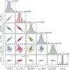 |
Fig. B.1. Corner plot showing the posterior distributions obtained for the fundamental stellar parameters and global asteroseismic parameters of Hennes. |
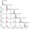 |
Fig. B.2. Corner plot displaying the posteriors obtained for the fundamental stellar parameters and global asteroseismic parameters from the modelling of Rogue. |
Appendix C: Fitting the global asteroseismic parameters
In order to emphasise the contrast to the previously best-possible case when asteroseismically modelling giant stars, we here present the results from a fit to the global asteroseismic parameters Δν, νmax, and ΔΠ1. The same classical parameters as in Sect. 5 are included in the fit. For Rogue, due to the reasons described in Sect. 3.2, we do not attempt to fit ΔΠ1.
Figures C.1 and C.2 show the Kiel diagrams for Hennes and Rogue, respectively. A clear lack of overlap between the observed constraint bands are seen, that is, a tension between the observables when translated to model space. This was the same situation that the prior efforts of V. Silva Aguirre et al. (unpublished) initially faced when performing the modelling attempts ten years ago. Tables C.1 and C.2 show the stellar parameters obtained for the modelling. Both Hennes and Rogue are recovered as vastly different stars from the ones found by modelling them utilising individual frequencies (see Sect 5). Note that the lower uncertainties recovered here, when compared to the ones found by the individual frequency modelling, occur due to the low uncertainties on the global asteroseismic parameters and the lacking overlap between them in model space.
Modelling results for Hennes when using global asteroseismic parameters.
Modelling results for Rogue when using global asteroseismic parameters.
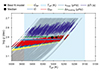 |
Fig. C.1. Kiel diagram of Hennes for a fit to the global asteroseismic parameters, displaying a representative number of stellar tracks in the grid. The observed constraints on the fitted parameters are overlaid to show a clear lack of overlap with the median and BFM from the posterior. |
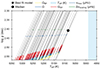 |
Fig. C.2. Kiel diagram of Rogue for a fit to the global asteroseismic parameters, displaying a representative number of stellar tracks in the grid. The observed constraints on the fitted parameters are overlaid to show a clear lack of overlap with the median and BFM from the posterior. |
A final interesting mention is that when we fit the global asteroseismic parameters but omit νmax, we can generally recover an overlap between the fitted constraints. This provides posteriors much more similar to the ones from individual frequency modelling. The posteriors are wider, which results in larger errors on the determined parameters, but encompasses the solution found by the individual frequency modelling. This further speaks to the unreliability of the νmax scaling relation for low-metallicity evolved stars (see Sect. 6.2).
Appendix D: Orbital Solutions for Hennes and Rogue
Table D.1 lists the orbital properties for Hennes and Rogue as described in Sect. 6. Therein, GC refers to Galactocentric quantities, while HC are heliocentric.
Summarised orbital parameters for Hennes and Rogue.
Appendix E: Frequency fitting algorithm of BASTA
In BASTA (Aguirre Børsen-Koch et al. 2022), the pipeline assesses the likelihood of a stellar model given the observational constraint of a set of individual mode frequencies in multiple steps.
In order to save computation time, BASTA can utilise the fact that the mode frequencies of the model and the observed mode frequencies need to be rather close for the likelihood to be significant. The user specifies a distance in frequency space, parametrised as a fraction of the observed large frequency separation. This distance is transformed into an asymmetric prior for which models only pass if the ℓ = 0 mode with the same radial order as the lowest observed radial mode is close to the observed counterpart. The asymmetric nature of this prior describes the expectation that due to the asteroseismic surface effect the model frequencies have greater values than the observed ones (Christensen-Dalsgaard et al. 1988).
As it is not guaranteed that all modes present in the star have observable visibilities, it is possible for a good model to have more modes than the set of observed frequencies, but not in reverse: a model that accurately describes the structure of the star cannot physically have a pattern of mode frequencies with less modes than what is observed, given that we believe every mode frequency in the set of observations to be real. Based on this principle, BASTA matches the observed modes to model counterparts using an algorithm that does not depend on the assigned mode identification of radial modes, but instead on the observed pattern. This is described in more detail in Aguirre Børsen-Koch et al. (2022) or alternatively in Sect. 3.1 of Ball et al. (2020), but briefly summarised BASTA matches the radial frequencies assuming that the radial order of the lowest radial mode is correct. Using the radial frequencies as boundaries for different segments and thus avoiding the issue that the surface effect can impact on matching in pure frequency space, it then matches the observed frequencies to model counterparts using the inverse mode inertia as a proxy for visibility (Benomar et al. 2014).
A single modification was made in this procedure for the results presented in this work, as we consider evolved RGB stars. The offset between the boundaries of the different sets is only applied if a single observed non-radial frequency is available, such as is the case for MS stars. However, as this work considers evolved RGB stars where all dipole modes are mixed modes with significant g-mode components, this frequency shift will result in unrealistic displacements of the ℓ = 1 modes during the matching. We have therefore forced the shift to be zero when matching the dipole modes, which is only enforced for Rogue, as we consider multiple dipole modes per acoustic mode order for Hennes. We note that these changes will impact the exact best-fitting model but not significantly the overall posterior distribution.
All Tables
Compiled spectroscopic determinations for Hennes and Rogue from various sources.
Global asteroseismic parameters for Hennes (KIC 4671239) and Rogue (KIC 7693833).
Parameter space of the tailored grids specifying the varied dimensions for Hennes and Rogue.
Estimates of the observed global asteroseismic parameters for Hennes and Rogue from the independent determinations.
All Figures
|
Fig. 1. Metallicity [Fe/H] plotted against the frequency of maximum oscillatory power νmax for known oscillating stars, adapted from the left panel of Fig. 2 from Huber et al. (2024). The shaded area represents the region of evolved RGB stars, with a boundary set at νmax ≲ 100 μHz. Noteworthy low-metallicity sub-giant branch (SGB) and RGB stars for which asteroseismic modelling has been performed are highlighted. Note that EPIC206443676 was modelled using the global asteroseismic parameters (Deheuvels et al. 2012), not the individual frequencies as in all other displayed cases. The red stars indicate the two giants considered in the present work. |
| In the text | |
|
Fig. 2. Power density spectrum of Hennes with the consolidated list of individual frequencies from Table A.2 overplotted. Both the raw spectrum (shaded gray) and a Gaussian smoothed version (black) are seen. The orange diamonds, green upwards, and blue downwards triangles depict the ℓ = 0, ℓ = 1, and ℓ = 2 modes, respectively. |
| In the text | |
|
Fig. 3. Observed power échelle diagram for Hennes with the consolidated list of individual frequencies from Table A.2 overplotted. The orange diamonds, green upwards, and blue downwards triangles depict the ℓ = 0, ℓ = 1, and ℓ = 2 modes, respectively. An offset has been applied to the x-axis for improved visualisation to avoid wrapping of the radial ridge. |
| In the text | |
|
Fig. 4. Power density spectrum of Rogue with the consolidated list of individual frequencies from Table A.3 overplotted. Both the raw spectrum and a Gaussian smoothed version are shown as the shaded gray and black spectra, respectively. The orange diamonds, green upwards, and blue downwards triangles depict the ℓ = 0, ℓ = 1, and ℓ = 2 modes, respectively. |
| In the text | |
|
Fig. 5. Observed power échelle diagram for Rogue with the consolidated list of individual frequencies from Table A.3 overplotted. The orange diamonds, green upwards, and blue downwards triangles depict the ℓ = 0, ℓ = 1, and ℓ = 2 modes, respectively. An offset has been applied to the x-axis for improved visualisation to avoid wrapping of the radial ridge. |
| In the text | |
|
Fig. 6. Échelle diagram of Hennes with the fitted individual frequencies matched to the modes of the best-fitting model. The orange diamonds, green upwards, and blue downwards triangles depict the ℓ = 0, ℓ = 1, and ℓ = 2 modes, respectively. The cubic term of the surface correction by Ball & Gizon (2014) has been applied to the model frequencies, with a surface correction coefficient of a3 = −7.0512 ⋅ 10−8. The size of the model modes is scaled related to the inverse of their respective inertia. An offset has been applied to the x-axis for improved visualisation to avoid wrapping of the radial ridge. |
| In the text | |
|
Fig. 7. Kiel diagram of Hennes displaying a representative number of stellar tracks in the grid. The observed constraints on the fitted parameters are overlaid to show an overlap with the median and best-fitting model from the posterior. |
| In the text | |
|
Fig. 8. Échelle diagram of Rogue with the fitted individual frequencies matched to the modes of the best-fitting model. The orange diamonds, green upwards, and blue downwards triangles depict the ℓ = 0, ℓ = 1, and ℓ = 2 modes, respectively. The cubic term of the surface correction by Ball & Gizon (2014) has been applied to the model modes, with a surface correction coefficient of a3 = −1.5554 ⋅ 10−7. The size of the model modes is scaled related to the inverse of their respective inertia. An offset has been applied to the x-axis for improved visualisation to avoid wrapping of the radial ridge. |
| In the text | |
|
Fig. 9. Kiel diagram of Rogue displaying a representative number of stellar tracks in the grid. The observed constraints on the fitted parameters are overlaid to show an overlap with the median and best-fitting model from the posterior. A clear discrepancy between the observed and modelled temperature is found, with the lower 1-σ uncertainty visualised by the boundary of the blue region. |
| In the text | |
|
Fig. 10. Propagation diagram for three stellar models depicting the characteristic frequencies in the interior near the lower convective boundary. The best-fitting model of Hennes is plotted alongside two models of similar evolutionary state, i.e. similar Δν value, with identical initial parameters except for a variation in [Fe/H]. The shaded region around the observed νmax of Hennes represents the extent of the evanescent region for the three models, which increases with metallicity. |
| In the text | |
|
Fig. 11. Integrated orbit of Rogue and Hennes within the Milky Way’s potential over a 10 Gyr period, depicted in Cartesian Galactocentric coordinates. The left panel presents a top-down view of the Galaxy (x, y), while the right panel shows an edge-on perspective (x, z). The Sun’s integrated orbit is included in both views as a reference. |
| In the text | |
|
Fig. 12. Toomre diagram showing the Galactic velocity components. The vertical axis represents motion perpendicular to the plane and the horizontal axis depicts motion within the plane. The location of Hennes and Rogue in this space are marked with red dots. The background density map represents the number count of single targets from Gaia DR3 with reliable astrometric data and available line-of-sight velocities (astrometric_params_solved = 95, non_single_star = 0, ruwe < 1.4, and rv_nb_transits > 0). |
| In the text | |
|
Fig. B.1. Corner plot showing the posterior distributions obtained for the fundamental stellar parameters and global asteroseismic parameters of Hennes. |
| In the text | |
|
Fig. B.2. Corner plot displaying the posteriors obtained for the fundamental stellar parameters and global asteroseismic parameters from the modelling of Rogue. |
| In the text | |
|
Fig. C.1. Kiel diagram of Hennes for a fit to the global asteroseismic parameters, displaying a representative number of stellar tracks in the grid. The observed constraints on the fitted parameters are overlaid to show a clear lack of overlap with the median and BFM from the posterior. |
| In the text | |
|
Fig. C.2. Kiel diagram of Rogue for a fit to the global asteroseismic parameters, displaying a representative number of stellar tracks in the grid. The observed constraints on the fitted parameters are overlaid to show a clear lack of overlap with the median and BFM from the posterior. |
| In the text | |
Current usage metrics show cumulative count of Article Views (full-text article views including HTML views, PDF and ePub downloads, according to the available data) and Abstracts Views on Vision4Press platform.
Data correspond to usage on the plateform after 2015. The current usage metrics is available 48-96 hours after online publication and is updated daily on week days.
Initial download of the metrics may take a while.