| Issue |
A&A
Volume 699, July 2025
|
|
|---|---|---|
| Article Number | A152 | |
| Number of page(s) | 27 | |
| Section | Stellar structure and evolution | |
| DOI | https://doi.org/10.1051/0004-6361/202453347 | |
| Published online | 04 July 2025 | |
Advancing the accuracy in age determinations of old-disk stars using an oscillating red giant in an eclipsing binary
1
Dipartimento di Fisica e Astronomia, Università di Bologna, Via Zamboni 33, Bologna 40126, Italy
2
Osservatorio di Astrofisica e Scienza dello Spazio di Bologna, INAF, Via Gobetti 93/3, Bologna 40129, Italy
3
Stellar Astrophysics Centre, Department of Physics and Astronomy, Aarhus University, Ny Munkegade 120, Aarhus C 8000, Denmark
4
School of Physics and Astronomy, University of Birmingham, B15 2TT Birmingham, United Kingdom
5
Osservatorio Astronomico di Padova, INAF, Vicolo dell’Osservatorio 5, Padova 35122, Italy
6
Research School of Astronomy & Astrophysics, Australian National University, Cotter Rd., Weston, ACT 2611, Australia
7
ARC Centre of Excellence for All Sky Astrophysics in 3 Dimensions (ASTRO 3D), Stromlo, Australia
8
Instituto de Astrofísica de Canarias, E-38205 La Laguna, Tenerife, Spain
9
Departamento de Astrofísica, Universidad de La Laguna, E-38206 La Laguna, Tenerife, Spain
10
Nordic Optical Telescope, Rambla José Ana Fernández Pérez 7, Breña Baja, La Palma 38711, Spain
11
Institut d’Astrophysique et Géophysique, l’Université de Liège, Allée du 6 août 17, Liège 4000, Belgium
12
LIRA, Observatoire de Paris, Université PSL, Sorbonne Université, Université Paris Cité, CY Cergy Paris Université, CNRS, 92190 Meudon, France
13
Astrophysics Group, Keele University, Staffordshire, ST5 5BG Newcastle-under-Lyme, United Kingdom
14
Department of Physics and Astronomy, University of Turku, Turku 20014, Finland
15
Department of Physics, P.O. Box 64 FI-00014 University of Helsinki, Helsinki, Finland
16
Armagh Observatory and Planetarium, College Hill, BT61 9DG Northern Ireland, UK
17
University of Craiova, Alexandru Ioan Cuza 13, Craiova 200585, Romania
18
CAHA, Observatorio de Calar Alto, Sierra de los Filabres, Gérgal 04550, Spain
19
GRANTECAN, Cuesta de San José s/n, E-38712 Breña Baja, La Palma, Spain
20
European Southern Observatory, Alonso de Cordova 3107, Vitacura, Santiago, Chile
⋆ Corresponding author: This email address is being protected from spambots. You need JavaScript enabled to view it.
Received:
8
December
2024
Accepted:
23
April
2025
Abstract
Context. The study of resonant oscillation modes in low-mass red giant branch stars enables us to infer their ages with exceptional (∼10%) precision. This unlocks the possibility to reconstruct the temporal evolution of the Milky Way at early cosmic times. Ensuring the accuracy of such a precise age scale is a fundamental but difficult challenge. Because the age of red giant branch stars primarily hinges on their mass, an independent mass determination for an oscillating red giant star provides the means for this assessment.
Aims. We analysed the old eclipsing binary KIC 10001167, which hosts an oscillating red giant branch star and is a member of the thick disk of the Milky Way. Of the known red giants in eclipsing binaries, this is the only member of the thick disk whose asteroseismic signal is of a high enough quality to test the seismic mass inference at the 2% level.
Methods. We measured the binary orbit and obtain fundamental stellar parameters through a combined analysis of light-curve eclipses and radial velocities, and we performed a detailed asteroseismic, photospheric, and Galactic kinematic characterisation of the red giant and the binary system.
Results. We show that the dynamically determined mass 0.9337 ± 0.0077 M⊙ (0.8%) of this 10 Gyr old star agrees within 1.4% with the mass inferred from a detailed modelling of individual pulsation mode frequencies (1.6%). This is now the only thick-disk stellar system that hosts a red giant for which the mass has been determined asteroseismically with a precision better than 2% and through a model-independent method at a precision of 1%. We hereby affirm the potential of asteroseismology to define an accurate age scale for ancient stars to trace the Milky Way assembly history.
Key words: binaries: eclipsing / stars: evolution / stars: fundamental parameters / stars: oscillations / stars: individual: KIC10001167 / Galaxy: disk
© The Authors 2025
 Open Access article, published by EDP Sciences, under the terms of the Creative Commons Attribution License (https://creativecommons.org/licenses/by/4.0), which permits unrestricted use, distribution, and reproduction in any medium, provided the original work is properly cited.
This article is published in open access under the Subscribe to Open model. This email address is being protected from spambots. You need JavaScript enabled to view it. to support open access publication.
1. Introduction
The precise age-dating of cosmic structures is one of the key challenges of modern astrophysics. The availability of chemo-dynamical constraints for millions of stars from the Gaia mission (Gaia Collaboration 2016) and large-scale spectroscopic surveys signified a step change in our understanding and identification of stellar populations that constitute the Milky Way (e.g., see Helmi 2020; Belokurov & Kravtsov 2022; Queiroz et al. 2023; Gaia Collaboration 2023a; Gallart et al. 2024). Moreover, information about disk galaxies at high redshift (z) is becoming available through observations with the JWST1 and ALMA2 (e.g., see Ferreira et al. 2023; Roman-Oliveira et al. 2023; Tsukui & Iguchi 2021), and we now have the possibility of comparing the high-z picture of galaxies with that given by the oldest of stars within our Galaxy for which we have exquisite high-resolution information about their dynamical and chemical composition. To chronologically connect these complementary views, we need a high (∼10%) temporal resolution, especially for the oldest tracers, that is, for stars with ages of ∼10 Gyr. Precise and accurate ages of the oldest objects in the Universe would also constitute a crucial test for modern cosmology (e.g., see Cimatti & Moresco 2023).
A significant step forward in the challenging task of inferring precise and accurate stellar ages (Soderblom 2010) has been provided by asteroseismology, which makes direct information about stellar interiors accessible for scientific investigation. Evolved low-mass stars showing solar-like oscillations represent ideal clocks to infer the chronology of the structure formation in the Milky Way, due to their intrinsic brightness and long main-sequence (MS) lifetimes (e.g., see Chaplin et al. 2020; Montalbán et al. 2021; Borre et al. 2022). The ages inferred using seismic constraints are often adopted as training sets to extend the age inference to hundreds of thousands of stars using machine-learning techniques applied to stellar spectroscopy, for example (e.g., see Anders et al. 2023, and references therein). An independent verification of the asteroseismic age scale is thus of paramount importance, since solar-like oscillating giants are starting to take on the role of primary calibrators to what is effectively becoming the cornerstone of the stellar age scale.
Because the age of red giant branch (RGB) stars is effectively their MS lifetime, which primarily depends on the initial mass (age ∝ M−α, with α ∼ 3 (e.g., see Kippenhahn et al. 2013), the reliability of the age scale of these stars is anchored to our ability to accurately measure their masses. In the past decade, several efforts were dedicated to comparing asteroseismically inferred masses with an independent determination of their masses available for stars in clusters (see Handberg et al. 2017; Brogaard et al. 2021, 2023, and references therein) and eclipsing binaries (see Gaulme et al. 2016; Brogaard et al. 2018, 2022; Themeßl et al. 2018; Thomsen et al. 2022, and references therein). While these independent measurements offer valuable tests, their precision or exploration of the parameter space are somewhat limited. This poses a significant obstacle especially for old low-mass metal-poor giants where independent and precise measurements are rare. For example, constraints from globular clusters are currently limited to a few giants with detectable oscillations using K2 data (e.g. Tailo et al. 2022; Howell et al. 2024), whose asteroseismic quality is significantly lower than that of Kepler, while the only other confirmed Kepler thick-disk eclipsing binary, KIC 4054905 (Gaulme et al. 2016; Brogaard et al. 2022), has significant light contamination and lower oscillation amplitudes. This effectively limits the asteroseismic precision in both cases such that it cannot challenge the mass accuracy at the typical 2% precision level achievable using individual mode frequencies from long-duration observations (Montalbán et al. 2021). A fundamental challenge is thus to obtain a model-independent mass determination with a percent-level precision for an old metal-poor red giant (RG) star showing well-determined solar-like oscillations.
In this context, the detached long-period eclipsing binary KIC 10001167 bears the hallmarks of the ideal benchmark for the mass and age scale of old stars. This system is bright (G = 10.05) and was observed for 4 years by the Kepler space satellite (Borucki et al. 2010). This provided an exquisite photometric monitoring, a detailed characterisation of the eclipses of its RG and MS component, and the detection of solar-like oscillations in its RG star. Moreover, KIC 10001167 was reported to be a spectroscopic double-lined binary by Gaulme et al. (2016), which enables a model-independent inference of the stellar component masses.
Gaulme et al. (2016) obtained a dynamical mass of 0.81 ± 0.05 M⊙ (6.2% precision) for the RG, however. This low value is puzzling because it would imply an age that exceeds the currently accepted age of the Universe, as noted by Brogaard et al. (2018). The low radial velocity (RV) precision of the Gaulme et al. (2016) study was explored in detail in previous works (Brogaard et al. 2018; Thomsen et al. 2022; Brogaard et al. 2022), and the poor sampling of the RV semi-amplitudes for this particular system has likely exacerbated this limitation. Moreover, an asteroseismic study of the individual oscillation modes of the star reported a mass of 0.94 ± 0.02 M⊙ (Montalbán et al. 2021), which is significantly higher and at a higher precision (2.1%) than the dynamical measurement. To investigate these potential discrepancies and limitations, we present revised dynamical mass measurements of the system components based on long-term high-precision RV monitoring, together with an in-depth spectroscopic, photometric, and asteroseismic analysis and modelling of the RG in the system.
2. Methods
The light-curve photometry we used was taken from the Kepler space mission (Borucki et al. 2010). For the spectroscopic characterisation and RV sampling of the binary orbit, we obtained 45 spectroscopic follow-up observations with the Fibre-fed Echelle Spectrograph (FIES) (Telting et al. 2014) at the Nordic Optical Telescope (NOT) on La Palma, which have a spectral resolution R ∼ 67 000. The spectral extraction and wavelength calibration was performed by the FIESTOOL (Stempels & Telting 2017) observatory pipeline.
The following sections describe the various methods we employed in our analysis. The RV measurement and separation of the stellar component spectra is presented in Sect. 2.1. The photospheric analysis of the RG through spectroscopy and photometry is presented in Sects. 2.2 and 2.4, respectively. Sect. 2.3 demonstrates the combined analyses of eclipse photometry and radial velocities. Sect. 2.5 outlines the Galactic kinematic analysis. Sect. 2.6 details the methods we used to obtain observational asteroseismic constraints for the RG. Finally, Sect. 2.7 illustrates the inference of the stellar parameters through comparison with stellar models.
2.1. Radial velocity and separation of the component spectra
For simultaneous RV measurements and spectral separation, we used the Python code sb2sep (v. 1.2.15) from Thomsen et al. (2022). It employs the broadening function formulation (Rucinski 2002) with synthetic templates from Coelho et al. (2005) for RVs and the spectral separation method of González & Levato (2006). To reduce instrumental drift, the wavelength solution was defined using a thorium-argon (ThAr) spectrum captured immediately before observation, and telluric RV corrections were applied. The barycentric corrections and barycentric Julian dates were calculated using BARYCORRPY (Kanodia & Wright 2018). The outputs from the separation and RV extraction are reported in Appendix Table K.1, while further details can be found in Appendix A. With a completely independent analysis method, outlined in Appendix B, we found consistent RV variation. Without (with) the jitter term we determine in Appendix A that was included in the binary orbit fit, the mean RV uncertainty is 29 (96) m/s for the RG and 0.48 (0.49) km/s for the MS star.
By separating the stellar components of the spectra, we obtained a high signal-to-noise ratio (S/N) stacked spectrum of the RG that is ideal for spectroscopic analysis. The separated component spectrum of the RG has a nominal S/N of ∼270 for the RG. The MS component spectrum is dominated by noise from the RG, and the quality is insufficient for an atmospheric analysis.
2.2. Spectral analysis
A detailed review on spectral analysis methods and their wide applications can be found in Nissen & Gustafsson (2018). The system was observed as part of the intermediate-resolution (R ∼ 22 500) near-infrared spectroscopic survey APOGEE DR17 (Abdurro’uf et al. 2022). Because we obtained a component spectrum of the RG of high resolution and S/N from the optical FIES spectra, we were able to perform an independent characterisation. The separated spectrum was renormalised using a wavelength-dependent light ratio derived from the Kepler passband light ratio obtained from the eclipsing binary analysis in Sect. 2.3. We assumed a blackbody spectral energy distribution, which is sufficient because the luminosity ratio is low  .
.
The stellar atmospheric parameters were then determined from classical equivalent width (EW) measurements obtained with DOOP (Daospec Output Optimiser pipeline, Cantat-Gaudin et al. 2014), which is a pipeline wrapper of DAOSPEC (Stetson & Pancino 2008). DAOSPEC is a FORTRAN program for the automatic recovery and identification of stellar absorption lines from an input line-list, continuum fitting, and EW measurement. To derive the atmospheric parameters from the EWs, we used FAMA (Fast Automatic MOOG Analysis, Magrini et al. 2013), which is an automated version of MOOG version 2017 (Sneden et al. 2012). This one-dimensional local thermal equilibrium radiative transfer code can be used to derive abundances from EWs through spectral synthesis. FAMA uses MOOG together with MARCS model atmospheres (Gustafsson et al. 2008). We fixed log g to the value inferred using the asteroseismic constraints, and we determined the other atmospheric parameters through the excitation equilibrium by minimising the trend between the reduced EW, log(EW/λ). FAMA computes elemental abundances using the MOOG routines ABFIND and BLENDS (see Magrini et al. 2013 for further details).
We used the line list given in Slumstrup et al. (2019), which was curated to avoid saturated lines and only includes lines with EW < 80 mÅ. It also includes astrophysically calibrated oscillator strengths. We compare astrophysical and laboratory oscillator strengths in Appendix C to validate our choice. We adopted a total uncertainty of 0.1 dex on [Fe/H] and [α/Fe] following the investigations of Bruntt et al. (2010) (see Table C.1 for the statistical uncertainty).
We obtained elemental abundance measurements of the neutral atomic lines NaI, MgI, AlI, SiI, CaI, TiI, CrI, FeI, and NiI and of the singly ionised lines TiII, FeII, as well as the logarithmic abundance of alpha-process elements, [α/Fe], here defined as ![Mathematical equation: $ \frac{1}{4}\left( [\rm Ca/Fe] + [\rm Si/Fe] + [\rm Mg/Fe] + [\rm Ti/Fe]\right) $](/articles/aa/full_html/2025/07/aa53347-24/aa53347-24-eq2.gif) . The solar abundances we used for our analysis are those from Asplund et al. (2009), while APOGEE DR17 used those by Grevesse et al. (2007). The elements are recorded in logarithmic abundance relative to iron in Table C.1, where we only list the statistical uncertainty. We note that the agreement with APOGEE DR17 on [Fe/H] is 0.05 dex, and it is better than ≲0.01 dex when the difference in solar scale is accounted for.
. The solar abundances we used for our analysis are those from Asplund et al. (2009), while APOGEE DR17 used those by Grevesse et al. (2007). The elements are recorded in logarithmic abundance relative to iron in Table C.1, where we only list the statistical uncertainty. We note that the agreement with APOGEE DR17 on [Fe/H] is 0.05 dex, and it is better than ≲0.01 dex when the difference in solar scale is accounted for.
2.3. Analysis of binarity
The analysis of spectroscopic double-lined binaries showing eclipses is a fundamental method of measuring precise and accurate stellar masses and radii (for an observational review, see e.g. Torres (2010), while a detailed theoretical background on the physics of advanced eclipsing binary modelling is available in Prša 2018). We performed two independent combined eclipsing light-curve and RV analyses using the codes JKTEBOP (v. 43, Southworth 2013) and PHysics Of Eclipsing BinariEs 2 (PHOEBE 2, Conroy et al. 2020). The properties of KIC 10001167 determined by our eclipsing binary analyses are presented in Table D.1. JKTEBOP is an eclipsing binary fitting code which offers high computational efficiency and numerical precision through a few key analytic approximations. In particular, during an eclipse, the two stellar components are assumed to be perfectly spherical, while during out-of-eclipse modelling, they can be treated as either spherical or bi-axial ellipsoids. PHOEBE 2 instead offers the possibility of relaxing several of these analytic approximations, thereby achieving higher accuracy for stars with significant deformation and reflection at the cost of a considerably lower computational efficiency. One of the main such features is the numerical approximation of the surface of the stars as a discrete mesh of connected triangles deformable by a Roche-lobe potential following Wilson (1979). It also includes internal handling of limb darkening, derived from a model atmosphere table for each mesh point, unlike JKTEBOP, where an analytic prescription must be assumed.
2.3.1. JKTEBOP
To analyse the eclipsing binary with JKTEBOP, we used the Kepler mission (Borucki et al. 2010) presearch data conditioning light curve (PDCSAP, Smith et al. 2017, and references therein)3. The choice of light curve is explained further in Appendix D.1, as is the pre-processing we performed, by normalising the eclipses with polynomial fitting, such that we could treat the stars as spherical during the JKTEBOP analysis.
We found no evidence of any background contamination from nearby stars (see Appendix D.1) or any indications of significant in-system contamination from the spectroscopy (see Appendix E). We applied the (h1, h2) parametrised power-2 limb-darkening law with coefficients interpolated from Claret & Southworth (2022), as the (h1, h2) parametrisation has been found to be superior to other two-parameter prescriptions when fitting for one coefficient (Maxted 2023). Further details can be found in Appendix D, in particular Appendix D.1, as well as Appendices D.2 and D.3, from which we estimated a systematic uncertainty of ∼0.7% for the radius of the RG from limb-darkening and atmosphere approximations.
An evaluation of the light-curve residuals around the best-fit demonstrates that they are dominated by stochastic solar-like oscillations rather than statistical noise. Therefore, following Thomsen et al. (2022), we employed a residual block bootstrap resampling method of the light curve to estimate the uncertainty. For the radial velocities, the sampling method also includes a Monte Carlo simulation in addition to residual resampling. This is a new addition since Thomsen et al. (2022).
The root mean square (RMS) of the residuals of our RVs from FIES is 0.097 km/s for the giant and 0.42 km/s for the MS component. There is a clear residual signal in the RVs of the RG after we subtracted the binary RV curve, which we investigate in Appendix B. Despite this additional signal, the S/N-limited precision of 0.42 km/s for the MS star RVs still dominates the stellar mass error budget. In Appendix D.4, we investigate the impact of light travel time and conclude that, while significant, it does not have to be accounted for to obtain accurate stellar parameters for this system.
2.3.2. PHOEBE 2
For the analysis with PHOEBE 2, we performed a custom iterative filtering of the KASOC light curve, inspired by Handberg & Lund (2014), in order to keep the full eclipsing binary signal. We explain our choice of light curve and describe the filtering in Appendix D.5.
Then, we performed an affine-invariant Markov chain Monte Carlo sampling (MCMC) with EMCEE (Foreman-Mackey et al. 2013), starting from the best-fit JKTEBOP solution. We found it necessary to heavily bin the data in order to reduce the computing time. We binned the data in time-space, with a two-day binning outside of the eclipses, no binning during eclipse ingress and egress, and a 0.3-day binning within the total and annular eclipse.
There is clear evidence of Doppler boosting/beaming in the light curve. While PHOEBE 2 does not officially support boosting in the current version due to numerical issues with its native interpolation of coefficients, we manually reenabled user-provided boosting coefficients to be supplied. This allowed us to sample it as a free parameter. This functionality will be made available in the next feature release v2.5 (Jones et al., in prep.). As a result of our sampling choice, Teff, RG was poorly constrained for this analysis because the boosting coefficient is completely uncoupled.
The uncertainties we obtained from the PHOEBE MCMC sampling are heavily underestimated due to the correlated (asteroseismic) un-modelled signal in the data (see Appendix D.5). Our JKTEBOP uncertainties should therefore be used instead for any comparison with other analyses, and we refer to the JKTEBOP result when we compare our results with asteroseismic and photometric inference.
We remark that the essential light-curve fit parameters of the two methods agree at 0.4σ for the sum of the fractional radii  , at 0.2σ for the radius ratio
  , and at 0.2σ for the inclination i (assuming the JKTEBOP uncertainties). These are the free parameters that are expected to be most significantly affected by the treatment of the stellar surface shape. For reference, the agreement on the radius of the giant is 0.4σ. This indicates that a spherical treatment of the stars during eclipse is sufficient for an accurate analysis of this system, provided that proper pre-processing of the light curve is performed.
2.4. Parallax, photometry, and IRFM
Gaia DR3 (Gaia Collaboration 2016, 2023b) offers parallax and optical photometry for KIC 10001167, and 2MASS (Skrutskie et al. 2010) provides near-infrared photometry. We present the main steps of our photometric analysis, and further details can be found in Appendix F. Table F.2 shows the astrometric parameters from Gaia DR3, including an additional uncertainty estimate due to the potential effect of the binary orbit, which we derive in Appendix F.1.
A detailed description of the infrared flux method (IRFM) can be found in Casagrande et al. (2006), but we summarise the principles here. Given a set of photometric observations covering a wide wavelength range, in our case Gaia DR3 BP, G, and RP, as well as 2MASS J, H, and Ks, the majority of the bolometric flux of the star can be measured directly. The remainder (typically 15–30%) is predicted with model fluxes (from Castelli & Kurucz 2003 in this work) to produce a bolometric correction assuming an initial effective temperature Teff. For a star of a given angular size θ, the IRFM exploits the strong sensitivity of the bolometric flux to Teff through the Stefan-Boltzmann law, while the infrared flux depends linearly on Teff through the Rayleigh-Jeans curve. This holds true for stars hotter than about 4000 K. The ratio of the bolometric to infrared flux can then be used to eliminate the dependence on θ, while preserving a good sensitivity to Teff (see e.g. Fig. 1 in Blackwell et al. 1979, for an illustration). A new Teff can thus be obtained, and the process can be iterated until convergence is reached in temperature. Because Teff and the bolometric flux are determined at each iteration, θ can also be computed.
Table F.1 includes photometric measurements of the RG derived using the parallax and the IRFM measurements with the implementation described by Casagrande et al. (2021), as well as single-passband luminosity estimates involving bolometric corrections (Casagrande & VandenBerg 2018, and references therein). While the IRFM is known to be nearly model independent and only mildly affected by the adopted metallicity and surface gravity (e.g. Casagrande et al. 2006, and references therein), it critically depends on the input photometry and reddening. For this analysis, we accounted for the two stellar components in the photometry using the radius ratio (JKTEBOP) and effective temperature ratio (PHOEBE) obtained from the eclipsing binary analysis. The reddening for this system is low and does not affect the results at the agreement level of the available dust maps, which we demonstrate in Appendices F.2, F.3. More details can be found in Appendix F.3.
2.5. Kinematics
We measured the Galactic position and velocities of KIC 10001167 using the distance derived from the parallax (see Appendix F.4), the celestial position and proper motions from Gaia DR3, and system RV from the JKTEBOP RG RV solution.
The Galactic orbital kinematics and the integrals of motion of the star were calculated using the GALPY fast orbit-estimation algorithm (Bovy 2015; Mackereth & Bovy 2018) by adopting the McMillan2017 potential (McMillan 2017). We assumed that the distance of the Sun to the Galactic centre is R⊙ = 8.2 kpc (McMillan 2017), and that the solar movement in the local standard of rest (LSR) frame is (U⊙, V⊙, W⊙) = (11.1, 12.24, 7.25) km s−1 (Schönrich et al. 2010) with vLSR = 221 km s−1. The uncertainties on the dynamical quantities were calculated using a bootstrap method, which involves randomly selecting a sample of phase-space quantities based on the given observational uncertainties and the covariance matrix associated with the Gaia parameters. In Table F.2 we list the astrometric and kinematic measurements.
2.6. Asteroseismic constraints
To measure the properties of the solar-like oscillation spectrum of KIC1000167, we used the KEPSEISMIC (e.g. Pires et al. 2015, and references therein) (from MAST3) and the KASOC photometric light curve, which were both designed for the asteroseismic analysis of giants. The KASOC light-curve pipeline employs a filtering technique made to remove transit signals (see Handberg & Lund 2014 for details), while the KEPSEISMIC light-curve version we used is filtered with an 80-day window.
2.6.1. Individual mode oscillation frequencies
We measured individual oscillation frequencies using four different combinations of pipelines and light-curve reductions. The methods are labelled with the power spectrum name (KEPSEISMIC or KASOC) and by the background and frequency extraction pipeline. The latter are either FAMED (Corsaro et al. 2020, and references therein), PBJam (Nielsen et al. 2021), or the frequency extraction method described by Arentoft et al. (2017). As background models describing stellar granulation, activity, and white noise, we either used a set of three Harvey-like profiles or the model described by Arentoft et al. (2017) (see Table G.1).
Our frequency measurements are detailed in Appendix G and are further described in Appendix G.2. The frequencies measured using different methods agree within ∼1σ, except for a few of those recovered by KEPSEISMIC+FAMED. We defined the reference set of frequencies to use in the modelling as that recovered with PBJam. During the later model inference, we compared with an inference performed using the set of frequencies showing the largest difference from PBJam (KEPSEISMIC+FAMED), and we treated it as a systematic source of uncertainty in the recovered stellar parameters.
Before they were used for the asteroseismic inference, the observed frequencies were corrected for the Doppler shift produced by the system line-of-sight velocity following Davies et al. (2014). However, due to the low pulsation frequencies of the modes, the shift is negligible in comparison to the frequency uncertainty.
2.6.2. Average asteroseismic parameters
Table G.1 shows measurements of the averaged asteroseismic parameters, the large frequency separation (Δν) and the frequency of maximum oscillation power (νmax), along with literature results for νmax. To determine Δν, we first used a power-spectrum stacking method (ΔνPS) and then refined it using only the individual radial-mode oscillation frequencies (Δν0) (Arentoft et al. 2017; Brogaard et al. 2021). νmax was obtained using the methods mentioned in Sect. 2.6.1. For the stellar parameter inference described below, a conservative estimate of νmax = 19.93 ± 0.47 μHz was adopted, which kept all the measurements in Table G.1 within 1σ.
2.7. Stellar parameter inference
The stellar parameters were inferred by comparing seismic and non-seismic observational constraints with predictions from models of the stellar structure and evolution. We employed two model grids based on different stellar evolution and pulsation codes.
The first grid was presented by Montalbán et al. (2021) and is based on the Liège stellar evolution code CLÉS (Scuflaire et al. 2008a). The stellar models were evolved from the pre-main-sequence up to a radius of 25 R⊙ on the RGB. Adiabatic oscillations of radial modes were computed with the code LOSC (Scuflaire et al. 2008b)4.
The second stellar model grid is described in detail in Tailo et al. (in prep.) and was computed using the stellar evolution software MESA (Paxton et al. 2019, and references therein) in its version n. 11701. Further details on the grid can also be found in Appendix G.1.
We used the code ’asteroseismic inference on a massive scale’ (AIMS; Rendle et al. 2019) to infer the stellar parameters and to explore the impact on the estimated mass and radius of using different combinations of observational constraints and uncertainties in the modelling. AIMS is a Bayesian parameter inference code that provides best-fitting stellar properties and full posterior probability distributions by comparing observational constraints with theoretical predictions from stellar models. It samples the parameter space using an MCMC method, and it includes interpolation routines capable of handling multi-dimensional irregularly sampled stellar model grids. For our asteroseismic inference, we supplied AIMS with observed individual oscillation frequencies extracted from the power spectrum, we constrained νmax (see Sect. 2.6.2), and we included an observational constraint on the effective temperature and surface metallicity (Z/X)surf. Using individual frequencies as observational constraints contributes to significantly reducing the uncertainties affecting estimated global stellar parameters. As demonstrated in several studies (e.g., see Gough 1990), theoretical individual-mode frequencies should be corrected for the so-called surface effects, that is, for systematic uncertainties stemming from our limited ability to model the near-surface layers of the star. We corrected for the theoretical frequencies using a two-term prescription following Ball & Gizon (2014, Eq. (4)), which involves two free parameters to be derived by the fitting procedure, a cubic a3 and an inverse term a−1 such that the correction δν becomes
![Mathematical equation: $$ \begin{aligned} \delta \nu (\nu , \mathcal{I} ) = \left[a_{-1}(\nu /\nu _{\rm ac})^{-1}+a_3(\nu /\nu _{\rm ac})^3\right]/\mathcal{I} , \end{aligned} $$](/articles/aa/full_html/2025/07/aa53347-24/aa53347-24-eq5.gif) (1)
(1)
where ν is the theoretical mode frequency, νac is the acoustic cut-off frequency, and ℐ is the normalised mode inertia. The other free parameters that were sampled are the stellar mass, the initial mass fraction of metals, and the stellar age. All other stellar parameters were derived from these or were held constant (when indicated), except for one fit, in which we explored the effect of varying the initial helium fraction Yi as well.
The main reference fit was obtained using the CLÉS grid ([α/Fe] = 0.3), with observational constraints from the six radial mode frequencies shown in Fig. 3 (obtained with PBJam), the quoted νmax value from Sect. 2.6.2, and the metallicity and effective temperature from APOGEE DR17. In Appendix G.3, we explore the effect of the choice of observational input in detail through several runs of AIMS and use this to infer realistic systematic uncertainties.
Finally, we also used AIMS to infer the age, including as observational constraints the dynamical mass and radius of the RG instead of the oscillation frequencies. To estimate the systematic uncertainties, we followed the same treatment as highlighted in the previous paragraph for the inferences using oscillation frequencies (variation in effective temperature and metallicity source, change to grid [α/Fe], and choice of stellar evolution code).
We also provide the asteroseismic scaling relation measurements in Appendix G.5, but we stress that scaling relations can be systematically much more uncertain than individual frequency inferences. We therefore do not focus on these results in the paper.
3. Results
In this section, we summarise the analysis results for KIC 10001167.
3.1. Spectroscopic, photometric, and kinematic analysis
Based on the photospheric chemical composition and on the Milky Way kinematics of KIC 10001167, Montalbán et al. (2021) classified it as a member of the Milky Way in situ high-[α/Fe] disk. In Fig. 1, KIC 10001167 is shown in the broader context of Milky Way giants observed by APOGEE DR17, where its combination of [Fe/H] and high [α/Fe] levels clearly distinguishes it from stars that were accreted from other galaxies (Helmi 2020), and it therefore is a prototypical in situ star. We note that its location in the [Mg/Mn]-[Al/Fe] plane, which has been shown to clearly separate in situ disk stars from those born ex situ (Das et al. 2020), further demonstrates its membership in the in situ thick disk.
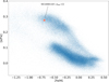 |
Fig. 1. α-enhancement level vs. iron abundance from APOGEE DR17 for stars with 1.5 < log g < 3. KIC 10001167 is highlighted. |
To provide additional and independent chemical constraints, we measured the iron abundance and detailed abundances of nine other elements using high-resolution spectroscopic data from the separated FIES spectrum of the RG. We found a logarithmic iron abundance of [Fe/H] = -0.73 ± 0.10 and an alpha-process element enhancement of [α/Fe]=+0.37 ± 0.10. This is compatible with APOGEE DR17, and it is an independent confirmation of the chemical association of the system with the old in situ disk. Further details of the method are available in Section 2.2.
Moreover, using astrometric constraints from Gaia DR3 (Gaia Collaboration 2023b) with our independent systemic RV measurement obtained from the FIES spectra, we found that the Galactic orbit of the star, in particular, its eccentricity of 0.42 ± 0.02 and orbital circularity of Lz/Lc = 0.8, with Lz being the orbital azimuthal angular momentum and Lc being the equivalent value for a circular orbit with the same energy, is compatible with an origin in the old in situ population (e.g. Chandra et al. 2024, and references therein).
Using photometric constraints from Gaia DR3 and 2MASS (Skrutskie et al. 2010), we measured a largely model-independent effective temperature and angular diameter of the RG with the infrared flux method (IRFM). The effective temperature of 4625 ± 29stat ± 30syst K is compatible with our spectroscopic analysis and with APOGEE DR17.
By combining our photometric IRFM measurement of the angular diameter with the Gaia DR3 parallax, we measured a radius of 12.82 ± 0.30stat ± 0.24syst R⊙ for the RG, where the systematic uncertainty includes the potential effect of the binary orbit on the parallax.
Our photospheric constraints for the RG can be found in Table 1, and a table with the detailed abundances can be found in Appendix Table C.1.
Measurements of the RG in KIC 10001167.
3.2. Analysis of binarity
The Kepler light curve shows clear eclipses of two stellar components and a signal from tidal deformation and Doppler beaming of the RG. This is demonstrated in Fig. 2 together with our spectroscopic follow-up RVs from FIES, including residual observed-calculated (O-C) plots.
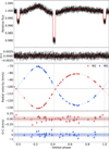 |
Fig. 2. Top: Binary signal in the light curve, along with the best-fit PHOEBE 2 model. Bottom: RV measurements and dynamical RV curves for the two stellar components. The dotted vertical lines indicate the location of eclipses. Both top and bottom panels include O-C residual sub-panels. |
To measure orbital and stellar parameters, we analysed the eclipsing binary light curve and RV together using two independent programs, JKTEBOP (Southworth 2013) for an analysis that only modelled the light-curve eclipses, and PHOEBE 2 (Conroy et al. 2020) for an analysis that incorporated tidal deformation and Doppler beaming. While the two codes have different underlying assumptions chiefly on stellar sphericity, we found an agreement on the RG radius of 0.4% (0.4σ) between them. Further details of the two analyses can be found in Section 2.3. All the measured orbital and stellar parameters are found in Appendix Table D.1.
With the eclipsing binary analysis, we measured the RG mass as 0.9337 ± 0.0077 M⊙ (0.8%) and its radius as 13.03 ± 0.12 R⊙ (0.9%). In Sect. 2.3.1, we furthermore estimate a potential systematic uncertainty of 0.7% for the RG radius from assumptions related to our treatment of the stellar atmosphere and limb darkening. Its value is quoted in Table 1.
3.3. Asteroseismic constraints and modelling
Figure 3 shows the frequency–power spectrum of the pre-processed light curve (see Section 2.6). The light curve from KIC10001167 presents a rich spectrum of overtones of solar-like oscillations from the RG. These modes are stochastically excited and intrinsically damped by near-surface convection. The modes may be decomposed onto spherical harmonics of angular degree ℓ. Overtones of radial (ℓ = 0), dipole (ℓ = 1) and quadrupole (ℓ = 2) modes are clearly seen. The structure of dipole modes is informative of the evolutionary state of the star (e.g. Bedding et al. 2011; Mosser et al. 2014), which supports previous analyses (Elsworth et al. 2019; Pinsonneault et al. 2018) that demonstrated that this star is in the RGB phase, that is in the hydrogen-shell burning phase, which follows the exhaustion of hydrogen in the stellar core (further details can be found in Appendix H). We measured the frequencies of individual radial and quadrupole modes using well-established data analysis procedures (Corsaro et al. 2020; Nielsen et al. 2021; Arentoft et al. 2017) (see Sect. 2.6 for further details).
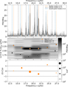 |
Fig. 3. Top: Frequency-power spectrum divided by the granulation background in the original (light) and uniformly smoothed (dark, window = 0.15 μHz). The vertical lines highlight the observed radial (ℓ = 0), dipole (ℓ = 1), and quadrupole (ℓ = 2) modes. Middle: Échelle diagram. The axes are flipped for illustration, showing observed radial ℓ = 0 and quadrupole ℓ = 2 frequencies and the best-fit frequencies from our reference radial mode fit. The heat-map data were uniformly smoothed with a window = 0.075 μHz. Bottom: Statistical significance of the O-C residuals relative to the measurement uncertainty σ. The marker-size was rescaled (in log10) to demonstrate the statistical weight 1/σ2 applied to each observed frequency in the asteroseismic inference. |
We then inferred the stellar properties using individual-mode frequencies and photospheric parameters from the IRFM and our optical spectroscopy or APOGEE DR17 as observational inputs in AIMS (Rendle et al. 2019). We extended the work of Montalbán et al. (2021) by exploring the impact of using different combinations of observational constraints and uncertainties in the modelling. We found a radius of 12.748 ± 0.068stat ± 0.055syst R⊙, a mass of 0.947 ± 0.015stat ± 0.009syst M⊙, and an age of 9.68 ± 0.64stat ± 0.56syst Gyr. This is consistent with the asteroseismic inference of Montalbán et al. (2021), who adopted a reduced set of oscillation frequencies and spectroscopic constraints from an earlier APOGEE data release.
The asteroseismic results are found to be robust against the systematic effects explored in Appendix G.3. We used different stellar structure and pulsation codes, different model temperature scales, including a Gaia-based luminosity, adopted abundances from APOGEE or from FIES, or by including quadrupole modes as observational constraints. We also performed an inversion for the mean stellar density following the approach described by Buldgen et al. (2019) and found the results to be consistent with those from the forward-modelling approach (see Appendix G.4).
In Appendix I we argue that it is unlikely that tidal effects have caused a significant bias in the asteroseismically determined radius.
In Appendix J we explore potential systematic effects related to mass loss during the RGB. They are similar to the currently adopted systematic uncertainty on the age.
When the mass and radius measurements from the eclipsing binary analysis are used as observational constraints instead of the seismic parameters, the recovered age is 10.33 ± 0.48stat ± 0.38syst Gyr, which is consistent at 1σ (6%) with the asteroseismic inference.
4. Discussion and conclusions
KIC 10001167 represents an exceptionally well-constrained binary system that is prototypical of stars that formed in the in situ high-[α/Fe] disk of the Milky Way at an iron abundance [Fe/H] ≃ −0.7 and [α/Fe] ∼ 0.3−0.4, meaning stars that predate any significant enrichment by type Ia supernovae (e.g., see Matteucci & Greggio 1986).
Based on our radial velocity monitoring program, we collected data that enabled us to measure the mass of the RG star in KIC 10001167 with a precision of 1%. Because the star is a low-luminosity giant, model-independent knowledge of its mass allowed us to infer an age from stellar models of 10.3 ± 0.5stat ± 0.3syst Gyr, independent of the available asteroseismic constraints.
In Fig. 4 we illustrate with two representative isochrones that the evolved nature of the RG ensures that knowledge of its mass is directly informative of the age of the system, regardless of the stellar luminosity, temperature, and radius.
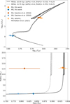 |
Fig. 4. Top: Hertzsprung-Russell diagram with the luminosity of the RG and MS from the eclipsing binary radius and the IRFM temperature (this work). The two isochrones shown were calculated from the MESA grid of stellar models used in this paper. We also include eclipsing binary measurements from Gaulme et al. (2016) and the asteroseismic inference of the RG from Montalbán et al. (2021). Bottom: Mass and radius of the same sources, along with the same isochrones. All markers have error bars in x and y, but in some cases, they are smaller than the marker. |
Fig. 5 illustrates the comparison between the mass, radius, and age for our measurements and the literature. We find that our asteroseismic mass measurements based on detailed seismic modelling agree with the dynamical mass at a level of 1.4%, which corresponds to 0.8σ, or 0.3σ when we account for systematic sources of uncertainty. Furthermore, Fig. 5 demonstrates that this ∼1σ difference in the measured mass directly matches the ∼1σ difference in inferred age between the two independent sets of observational constraints (eclipsing binary and asteroseismic), as expected.
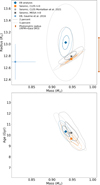 |
Fig. 5. Top: RG mass vs. radius measurements from this work and from the literature. The contours represent one and two sigma. As guides, circles are drawn around our eclipsing binary measurement representing a 2 and 5% radial difference in mass and radius. The arrow represents ±1σ for the radius measurement with the infrared flux method and Gaia DR3 parallax. Bottom: Mass vs. age from the stellar model inferences. |
The asteroseismically inferred photospheric radius was found to agree within 2.1% with the dynamical radius (2.1σ). When we considered the systematics in the two analyses, however, the difference between the measurements may be as small as 1.1σ. Further research is needed to ascertain the significance of this difference, which also affects the inferred mean density. This includes a thorough evaluation of the systematic errors associated with the current treatments of the stellar atmosphere in eclipsing binary models for giants, especially the limb-darkening prescriptions. The independent photospheric radius obtained with the IRFM and the Gaia DR3 parallax, with its precision of 2.3%, is compatible with the two measures within 1σ.
While independent checks of asteroseismically inferred radii (and hence distances) can also be performed using precise Gaia parallaxes for thousands of stars (e.g., see Khan et al. 2023, and references therein), high-accuracy comparisons between independent stellar mass determinations are unique to binaries. In this context, the percent-level agreement on mass we obtained for KIC 10001167 demonstrates that asteroseismic inferences using individual oscillation modes provide a method for achieving not only high-precision (2%, see Montalbán et al. 2021), but also high-accuracy measurements of masses and ages for thousands of the oldest RGB stars in the Milky Way. We thus demonstrated that asteroseismology offers the opportunity to accurately probe the assembly history of the Milky Way at early cosmic times. Asteroseismology can further be used to establish a fundamental training set for data-driven techniques, enabling the inference of ages for millions of stars with a truly improved temporal resolution that we are currently lacking.
It remains critically important to extend the sample of fundamental mass and age calibrators. Currently, KIC 10001167 is the only old-disk RG hosting binary with the necessary asteroseismic and dynamical constraints for these detailed comparisons. However, the upcoming mission PLATO (Rauer et al. 2014, 2025; Miglio et al. 2017) has the potential to increase this sample, and Gaia will also contribute to it with astrometric binaries (Beck et al. 2024). Finally, further tests of the reliability of stellar models, as well as the asteroseismic age and mass scales in different Galactic environments and stellar clusters (as envisioned by the HAYDN mission Miglio et al. 2021a) will help us to further enhance the time resolution with which we can study the history of the Milky Way.
The James Webb Space Telescope.
The Atacama Large Millimeter Array.
The grid, together with a description of its key input physics, is available at https://zenodo.org/records/4032320
We use ESPRESSO(Pepe et al. 2021) line masks, which have been published on https://www.eso.org
Saltire python code and documentation is available on Github.
Acknowledgments
JST acknowledge support from Bologna University, “MUR FARE Grant Duets CUP J33C21000410001”. KB, JM, MT, GC, AM, MM acknowledge support from the ERC Consolidator Grant funding scheme (project ASTEROCHRONOMETRY, https://www.asterochronometry.eu, G.A. n. 772293). Funding for the Stellar Astrophysics Centre is provided by The Danish National Research Foundation (Grant agreement no.: DNRF106). Based on observations made with the Nordic Optical Telescope, owned in collaboration by the University of Turku and Aarhus University, and operated jointly by Aarhus University, the University of Turku and the University of Oslo, representing Denmark, Finland and Norway, the University of Iceland and Stockholm University at the Observatorio del Roque de los Muchachos, La Palma, Spain, of the Instituto de Astrofisica de Canarias. This research is also supported by work funded from the European Research Council (ERC), the European Union’s Horizon 2020 research, and innovation programme (grant agreement n°803193/BEBOP). DJ acknowledges support from the Agencia Estatal de Investigación del Ministerio de Ciencia, Innovación y Universidades (MCIU/AEI) and the European Regional Development Fund (ERDF) with reference PID-2022-136653NA-I00 (DOI:10.13039/501100011033). DJ also acknowledges support from the Agencia Estatal de Investigación del Ministerio de Ciencia, Innovación y Universidades (MCIU/AEI) and the European Union NextGenerationEU/PRTR with reference CNS2023-143910 (DOI:10.13039/501100011033). GB acknowledges funding from the Fonds National de la Recherche Scientifique (FNRS) as a postdoctoral researcher. This work was supported by the UK Science and Technology Facilities Council under grant number ST/Y002563/1. This paper includes data collected by the Kepler mission. Funding for the Kepler mission is provided by the NASA Science Mission directorate.
References
- Abdurro’uf, Accetta, K., Aerts, C., et al. 2022, ApJS, 259, 35 [NASA ADS] [CrossRef] [Google Scholar]
- Anders, F., Gispert, P., Ratcliffe, B., et al. 2023, A&A, 678, A158 [NASA ADS] [CrossRef] [EDP Sciences] [Google Scholar]
- Arentoft, T., Brogaard, K., Jessen-Hansen, J., et al. 2017, ApJ, 838, 115 [NASA ADS] [CrossRef] [Google Scholar]
- Asplund, M., Grevesse, N., Sauval, A. J., & Scott, P. 2009, ARA&A, 47, 481 [NASA ADS] [CrossRef] [Google Scholar]
- Bailer-Jones, C. A. L., Rybizki, J., Fouesneau, M., Demleitner, M., & Andrae, R. 2021, AJ, 161, 147 [Google Scholar]
- Ball, W. H., & Gizon, L. 2014, A&A, 568, A123 [NASA ADS] [CrossRef] [EDP Sciences] [Google Scholar]
- Ball, W. H., Chaplin, W. J., Schofield, M., et al. 2018, ApJS, 239, 34 [Google Scholar]
- Baycroft, T. A., Triaud, A. H. M. J., Faria, J., Correia, A. C. M., & Standing, M. R. 2023, MNRAS, 521, 1871 [Google Scholar]
- Beck, P. G., Grossmann, D. H., Steinwender, L., et al. 2024, A&A, 682, A7 [NASA ADS] [CrossRef] [EDP Sciences] [Google Scholar]
- Bedding, T. R., Mosser, B., Huber, D., et al. 2011, Nature, 471, 608 [Google Scholar]
- Belokurov, V., & Kravtsov, A. 2022, MNRAS, 514, 689 [NASA ADS] [CrossRef] [Google Scholar]
- Blackwell, D. E., Shallis, M. J., & Selby, M. J. 1979, MNRAS, 188, 847 [NASA ADS] [CrossRef] [Google Scholar]
- Borre, C. C., Aguirre Børsen-Koch, V., Helmi, A., et al. 2022, MNRAS, 514, 2527 [NASA ADS] [CrossRef] [Google Scholar]
- Borucki, W. J., Koch, D., Basri, G., et al. 2010, Science, 327, 977 [Google Scholar]
- Bovy, J. 2015, ApJS, 216, 29 [NASA ADS] [CrossRef] [Google Scholar]
- Brogaard, K., Hansen, C. J., Miglio, A., et al. 2018, MNRAS, 476, 3729 [Google Scholar]
- Brogaard, K., Pakštienė, E., Grundahl, F., et al. 2021, A&A, 645, A25 [NASA ADS] [CrossRef] [EDP Sciences] [Google Scholar]
- Brogaard, K., Arentoft, T., Slumstrup, D., et al. 2022, A&A, 668, A82 [NASA ADS] [CrossRef] [EDP Sciences] [Google Scholar]
- Brogaard, K., Arentoft, T., Miglio, A., et al. 2023, A&A, 679, A23 [NASA ADS] [CrossRef] [EDP Sciences] [Google Scholar]
- Brogaard, K., Miglio, A., van Rossem, W. E., Willett, E., & Thomsen, J. S. 2024, A&A, 691, A288 [NASA ADS] [CrossRef] [EDP Sciences] [Google Scholar]
- Bruntt, H., Bedding, T. R., Quirion, P.-O., et al. 2010, MNRAS, 405, 1907 [NASA ADS] [Google Scholar]
- Buldgen, G., Rendle, B., Sonoi, T., et al. 2019, MNRAS, 482, 2305 [Google Scholar]
- Cantat-Gaudin, T., Donati, P., Pancino, E., et al. 2014, A&A, 562, A10 [NASA ADS] [CrossRef] [EDP Sciences] [Google Scholar]
- Casagrande, L., & VandenBerg, D. A. 2018, MNRAS, 479, L102 [NASA ADS] [CrossRef] [Google Scholar]
- Casagrande, L., Portinari, L., & Flynn, C. 2006, MNRAS, 373, 13 [Google Scholar]
- Casagrande, L., Lin, J., Rains, A. D., et al. 2021, MNRAS, 507, 2684 [NASA ADS] [CrossRef] [Google Scholar]
- Castelli, F., & Kurucz, R. L. 2003, in Modelling of Stellar Atmospheres, eds. N. Piskunov, W. W. Weiss, & D. F. Gray, IAU Symposium, 210, A20 [Google Scholar]
- Chandra, V., Semenov, V. A., Rix, H.-W., et al. 2024, ApJ, 972, 112 [Google Scholar]
- Chaplin, W. J., Serenelli, A. M., Miglio, A., et al. 2020, Nat. Astron., 4, 382 [Google Scholar]
- Cimatti, A., & Moresco, M. 2023, ApJ, 953, 149 [NASA ADS] [CrossRef] [Google Scholar]
- Claret, A., & Bloemen, S. 2011, A&A, 529, A75 [NASA ADS] [CrossRef] [EDP Sciences] [Google Scholar]
- Claret, A., & Southworth, J. 2022, A&A, 664, A128 [NASA ADS] [CrossRef] [EDP Sciences] [Google Scholar]
- Claret, A., & Southworth, J. 2023, A&A, 674, A63 [NASA ADS] [CrossRef] [EDP Sciences] [Google Scholar]
- Coelho, P., Barbuy, B., Meléndez, J., Schiavon, R. P., & Castilho, B. V. 2005, A&A, 443, 735 [NASA ADS] [CrossRef] [EDP Sciences] [Google Scholar]
- Conroy, K. E., Kochoska, A., Hey, D., et al. 2020, ApJS, 250, 34 [Google Scholar]
- Corsaro, E., McKeever, J. M., & Kuszlewicz, J. S. 2020, A&A, 640, A130 [NASA ADS] [CrossRef] [EDP Sciences] [Google Scholar]
- Cox, J. P., & Giuli, R. T. 1968, Principles of stellar structure (New York: Gordon and Breach) [Google Scholar]
- Das, P., Hawkins, K., & Jofré, P. 2020, MNRAS, 493, 5195 [NASA ADS] [CrossRef] [Google Scholar]
- Davies, G. R., Handberg, R., Miglio, A., et al. 2014, MNRAS, 445, L94 [NASA ADS] [CrossRef] [Google Scholar]
- Dréau, G., Mosser, B., Lebreton, Y., Gehan, C., & Kallinger, T. 2021, A&A, 650, A115 [NASA ADS] [CrossRef] [EDP Sciences] [Google Scholar]
- Elsworth, Y., Hekker, S., Johnson, J. A., et al. 2019, MNRAS, 489, 4641 [NASA ADS] [CrossRef] [Google Scholar]
- Faria, J. P., Santos, N. C., Figueira, P., & Brewer, B. J. 2018, J. Open Source Softw., 3, 487 [NASA ADS] [CrossRef] [Google Scholar]
- Ferreira, L., Conselice, C. J., Sazonova, E., et al. 2023, ApJ, 955, 94 [NASA ADS] [CrossRef] [Google Scholar]
- Foreman-Mackey, D., Hogg, D. W., Lang, D., & Goodman, J. 2013, PASP, 125, 306 [Google Scholar]
- Gaia Collaboration (Prusti, T., et al.) 2016, A&A, 595, A1 [NASA ADS] [CrossRef] [EDP Sciences] [Google Scholar]
- Gaia Collaboration (Recio-Blanco, A., et al.) 2023a, A&A, 674, A38 [CrossRef] [EDP Sciences] [Google Scholar]
- Gaia Collaboration (Vallenari, A., et al.) 2023b, A&A, 674, A1 [NASA ADS] [CrossRef] [EDP Sciences] [Google Scholar]
- Gallart, C., Surot, F., Cassisi, S., et al. 2024, A&A, 687, A168 [NASA ADS] [CrossRef] [EDP Sciences] [Google Scholar]
- Gaulme, P., McKeever, J., Jackiewicz, J., et al. 2016, ApJ, 832, 121 [NASA ADS] [CrossRef] [Google Scholar]
- González, J. F., & Levato, H. 2006, A&A, 448, 283 [NASA ADS] [CrossRef] [EDP Sciences] [Google Scholar]
- Gough, D. O. 1990, in Progress of Seismology of the Sun and Stars, eds. Y. Osaki, & H. Shibahashi, 367, 283 [Google Scholar]
- Green, G. M. 2018, J. Open Source Softw., 3, 695 [Google Scholar]
- Green, G. M., Schlafly, E., Zucker, C., Speagle, J. S., & Finkbeiner, D. 2019, ApJ, 887, 93 [NASA ADS] [CrossRef] [Google Scholar]
- Grevesse, N., Asplund, M., & Sauval, A. J. 2007, Space Sci. Rev., 130, 105 [Google Scholar]
- Gustafsson, B., Edvardsson, B., Eriksson, K., et al. 2008, A&A, 486, 951 [NASA ADS] [CrossRef] [EDP Sciences] [Google Scholar]
- Handberg, R., & Lund, M. N. 2014, MNRAS, 445, 2698 [Google Scholar]
- Handberg, R., Brogaard, K., Miglio, A., et al. 2017, MNRAS, 472, 979 [CrossRef] [Google Scholar]
- Hekker, S., Broomhall, A. M., Chaplin, W. J., et al. 2010, MNRAS, 402, 2049 [NASA ADS] [CrossRef] [Google Scholar]
- Helmi, A. 2020, ARA&A, 58, 205 [Google Scholar]
- Howell, M., Campbell, S. W., Stello, D., & De Silva, G. M. 2024, MNRAS, 527, 7974 [Google Scholar]
- Huber, D., Stello, D., Bedding, T. R., et al. 2009, CoAst, 160, 74 [NASA ADS] [Google Scholar]
- Husser, T. O., Wende-von Berg, S., Dreizler, S., et al. 2013, A&A, 553, A6 [NASA ADS] [CrossRef] [EDP Sciences] [Google Scholar]
- Kallinger, T. 2019, arXiv e-prints [arXiv:1906.09428] [Google Scholar]
- Kallinger, T., Mosser, B., Hekker, S., et al. 2010, A&A, 522, A1 [NASA ADS] [CrossRef] [EDP Sciences] [Google Scholar]
- Kalman, D. 1996, Coll. Math. J., 27, 2 [Google Scholar]
- Kanodia, S., & Wright, J. 2018, Res. Notes Am. Astron. Soc., 2, 4 [Google Scholar]
- Khan, S., Miglio, A., Willett, E., et al. 2023, A&A, 677, A21 [NASA ADS] [CrossRef] [EDP Sciences] [Google Scholar]
- Kippenhahn, R., Weigert, A., & Weiss, A. 2013, Stellar Structure and Evolution (Berlin, Heidelberg: Springer Berlin Heidelberg) [Google Scholar]
- Krishna Swamy, K. S. 1966, ApJ, 145, 174 [Google Scholar]
- Lallement, R., Babusiaux, C., Vergely, J. L., et al. 2019, A&A, 625, A135 [NASA ADS] [CrossRef] [EDP Sciences] [Google Scholar]
- Lallement, R., Vergely, J. L., Babusiaux, C., & Cox, N. L. J. 2022, A&A, 661, A147 [NASA ADS] [CrossRef] [EDP Sciences] [Google Scholar]
- Lightkurve Collaboration (Cardoso, J. V. d. M., et al.) 2018, Astrophysics Source Code Library [record ascl:1812.013] [Google Scholar]
- Lindegren, L., Bastian, U., Biermann, M., et al. 2021, A&A, 649, A4 [EDP Sciences] [Google Scholar]
- Mackereth, J. T., & Bovy, J. 2018, PASP, 130, 114501 [Google Scholar]
- Magrini, L., Randich, S., Friel, E., et al. 2013, A&A, 558, A38 [NASA ADS] [CrossRef] [EDP Sciences] [Google Scholar]
- Maíz Apellániz, J., Pantaleoni González, M., & Barbá, R. H. 2021, A&A, 649, A13 [NASA ADS] [CrossRef] [EDP Sciences] [Google Scholar]
- Matteucci, F., & Greggio, L. 1986, A&A, 154, 279 [NASA ADS] [Google Scholar]
- Matteuzzi, M., Montalbán, J., Miglio, A., et al. 2023, A&A, 671, A53 [NASA ADS] [CrossRef] [EDP Sciences] [Google Scholar]
- Maxted, P. F. L. 2016, A&A, 591, A111 [NASA ADS] [CrossRef] [EDP Sciences] [Google Scholar]
- Maxted, P. F. L. 2023, MNRAS, 522, 2683 [NASA ADS] [CrossRef] [Google Scholar]
- McMillan, P. J. 2017, MNRAS, 465, 76 [NASA ADS] [CrossRef] [Google Scholar]
- Miglio, A., Chiappini, C., Mosser, B., et al. 2017, Astron. Nachr., 338, 644 [Google Scholar]
- Miglio, A., Girardi, L., Grundahl, F., et al. 2021a, Exp. Astron., 51, 963 [NASA ADS] [CrossRef] [Google Scholar]
- Miglio, A., Chiappini, C., Mackereth, J. T., et al. 2021b, A&A, 645, A85 [NASA ADS] [CrossRef] [EDP Sciences] [Google Scholar]
- Montalbán, J., Mackereth, J. T., Miglio, A., et al. 2021, Nat. Astron., 5, 640 [Google Scholar]
- Mosser, B., & Appourchaux, T. 2009, A&A, 508, 877 [NASA ADS] [CrossRef] [EDP Sciences] [Google Scholar]
- Mosser, B., Goupil, M. J., Belkacem, K., et al. 2012, A&A, 540, A143 [NASA ADS] [CrossRef] [EDP Sciences] [Google Scholar]
- Mosser, B., Benomar, O., Belkacem, K., et al. 2014, A&A, 572, L5 [NASA ADS] [CrossRef] [EDP Sciences] [Google Scholar]
- Nielsen, M. B., Davies, G. R., Ball, W. H., et al. 2021, AJ, 161, 62 [NASA ADS] [CrossRef] [Google Scholar]
- Nissen, P. E., & Gustafsson, B. 2018, A&ARv, 26, 6 [Google Scholar]
- Ong, J. M. J., & Basu, S. 2020, ApJ, 898, 127 [NASA ADS] [CrossRef] [Google Scholar]
- Paxton, B., Smolec, R., Schwab, J., et al. 2019, ApJS, 243, 10 [Google Scholar]
- Pecaut, M. J., & Mamajek, E. E. 2013, ApJS, 208, 9 [Google Scholar]
- Pepe, F., Cristiani, S., Rebolo, R., et al. 2021, A&A, 645, A96 [NASA ADS] [CrossRef] [EDP Sciences] [Google Scholar]
- Pinsonneault, M. H., Elsworth, Y. P., Tayar, J., et al. 2018, ApJS, 239, 32 [Google Scholar]
- Pires, S., Mathur, S., García, R. A., et al. 2015, A&A, 574, A18 [NASA ADS] [CrossRef] [EDP Sciences] [Google Scholar]
- Prša, A. 2018, Modeling and Analysis of Eclipsing Binary Stars; The theory and design principles of PHOEBE (Bristol, UK: IOP Publishing) [Google Scholar]
- Prša, A., Harmanec, P., Torres, G., et al. 2016, AJ, 152, 41 [Google Scholar]
- Queiroz, A. B. A., Anders, F., Chiappini, C., et al. 2023, A&A, 673, A155 [NASA ADS] [CrossRef] [EDP Sciences] [Google Scholar]
- Queloz, D., Henry, G. W., Sivan, J. P., et al. 2001, A&A, 379, 279 [NASA ADS] [CrossRef] [EDP Sciences] [Google Scholar]
- Rappaport, S. A., Borkovits, T., Gagliano, R., et al. 2022, MNRAS, 513, 4341 [NASA ADS] [CrossRef] [Google Scholar]
- Rauer, H., Catala, C., Aerts, C., et al. 2014, Exp. Astron., 38, 249 [Google Scholar]
- Rauer, H., Aerts, C., Cabrera, J., et al. 2025, Exp. Astron., 59, 26 [Google Scholar]
- Reimers, D. 1975, Mem. Soc. R. Sci. Liege., 8, 369 [Google Scholar]
- Rendle, B. M., Buldgen, G., Miglio, A., et al. 2019, MNRAS, 484, 771 [Google Scholar]
- Rodrigues, T. S., Bossini, D., Miglio, A., et al. 2017, MNRAS, 467, 1433 [NASA ADS] [Google Scholar]
- Roman-Oliveira, F., Fraternali, F., & Rizzo, F. 2023, MNRAS, 521, 1045 [NASA ADS] [CrossRef] [Google Scholar]
- Rucinski, S. M. 2002, AJ, 124, 1746 [Google Scholar]
- Schönrich, R., Binney, J., & Dehnen, W. 2010, MNRAS, 403, 1829 [NASA ADS] [CrossRef] [Google Scholar]
- Scuflaire, R., Théado, S., Montalbán, J., et al. 2008a, Ap&SS, 316, 83 [Google Scholar]
- Scuflaire, R., Montalbán, J., Théado, S., et al. 2008b, Ap&SS, 316, 149 [Google Scholar]
- Sebastian, D., Triaud, A. H. M. J., & Brogi, M. 2024a, MNRAS, 527, 10921 [Google Scholar]
- Sebastian, D., Triaud, A. H. M. J., Brogi, M., et al. 2024b, MNRAS, 530, 2572 [Google Scholar]
- Sharma, S., Stello, D., Bland-Hawthorn, J., Huber, D., & Bedding, T. R. 2016, ApJ, 822, 15 [Google Scholar]
- Sing, D. K. 2010, A&A, 510, A21 [NASA ADS] [CrossRef] [EDP Sciences] [Google Scholar]
- Skrutskie, M. F., Cutri, R. M., Stiening, R., et al. AJ, 131, 1163 [Google Scholar]
- Slumstrup, D., Grundahl, F., Silva Aguirre, V., & Brogaard, K. 2019, A&A, 622, A111 [NASA ADS] [CrossRef] [EDP Sciences] [Google Scholar]
- Smith, J. C., Stumpe, M. C., Jenkins, J. M., et al. 2017, in Kepler Data Processing Handbook: Presearch Data Conditioning, Kepler Science Document KSCI-19081-002, ed. J. M. Jenkins, 8 [Google Scholar]
- Sneden, C., Bean, J., Ivans, I., Lucatello, S., & Sobeck, J. 2012, Astrophysics Source Code Library [record ascl:1202.009] [Google Scholar]
- Soderblom, D. R. 2010, ARA&A, 48, 581 [Google Scholar]
- Sonoi, T., Samadi, R., Belkacem, K., et al. 2015, A&A, 583, A112 [NASA ADS] [CrossRef] [EDP Sciences] [Google Scholar]
- Southworth, J. 2013, A&A, 557, A119 [NASA ADS] [CrossRef] [EDP Sciences] [Google Scholar]
- Southworth, J. 2023, Observatory, 143, 71 [Google Scholar]
- Stempels, E., & Telting, J. 2017, Astrophysics Source Code Library [record ascl:1708.009] [Google Scholar]
- Stetson, P. B., & Pancino, E. 2008, PASP, 120, 1332 [Google Scholar]
- Tailo, M., Corsaro, E., Miglio, A., et al. 2022, A&A, 662, L7 [NASA ADS] [CrossRef] [EDP Sciences] [Google Scholar]
- Telting, J. H., Avila, G., Buchhave, L., et al. 2014, Astron. Nachr., 335, 41 [Google Scholar]
- Themeßl, N., Hekker, S., Southworth, J., et al. 2018, MNRAS, 478, 4669 [Google Scholar]
- Thomsen, J. S., Brogaard, K., Arentoft, T., et al. 2022, MNRAS, 517, 4187 [NASA ADS] [CrossRef] [Google Scholar]
- Torres, G. 2010, AJ, 140, 1158 [Google Scholar]
- Townsend, R. H. D., & Teitler, S. A. 2013, MNRAS, 435, 3406 [Google Scholar]
- Tsukui, T., & Iguchi, S. 2021, Science, 372, 1201 [NASA ADS] [CrossRef] [Google Scholar]
- Verbunt, F., & Phinney, E. S. 1995, A&A, 296, 709 [NASA ADS] [Google Scholar]
- Vrard, M., Kallinger, T., Mosser, B., et al. 2018, A&A, 616, A94 [NASA ADS] [CrossRef] [EDP Sciences] [Google Scholar]
- Wilson, R. E. 1979, ApJ, 234, 1054 [Google Scholar]
- Yu, J., Huber, D., Bedding, T. R., et al. 2018, ApJS, 236, 42 [NASA ADS] [CrossRef] [Google Scholar]
Appendix A: Radial velocity analysis details
Detailed outputs from the separation and RV analysis are reported in Appendix Table K.1. For spectral separation, each spectrum is weighted according to its exposure time, as well as component RV separation and eclipse occurrence. We calculate RV corrections based on the wavelength positions of telluric lines, by cross-correlating the strong telluric lines at 6865–6925Å. We estimate RV uncertainties by combining in quadrature the following uncertainty estimates: 1. Internal uncertainty from stellar RV measured on smaller wavelength intervals, corrected for a linear instrumental trend with wavelength for the RG likely caused by systematics in either the instrumental line profile or the wavelength solution (RG mean 21 m/s, MS mean 0.39 km/s). 2. Local night-to-night scatter in the cross-correlation of the ThAr spectra, not considering long-term trends (6 − 9 m/s). 3. Cross-validation uncertainty estimate for the telluric corrections (11 − 44 m/s). 4. A fixed RV jitter uncertainty from correlated noise, evaluated from the best-fit JKTEBOP RG residuals (91 m/s). Excluding (including) jitter, we find a mean RV uncertainty of 29 (96) m/s for the RG and 0.48 (0.49) km/s for the MS star.
Appendix B: Radial velocity verification
In Sect. 2.3, we find the presence of an additional signal in the RVs of the RG beside classical two-body Keplerian motion. We rule out long-term variations in the Keplerian orbit as the sole cause of this (e.g. eccentricity change, period change, or tidal apsidal motion) by trial fitting with perturbed models. Line profile variations for the RG could potentially explain some of the behaviour. Non-Keplerian Doppler shifts e.g. pulsations, or a perturbing long-period circumbinary component, can each account for parts of the signal but cannot be proven without a longer baseline.
We compare our measured RVs to a newly developed method, which allows us to measure both components of high-contrast binaries using cross-correlation with a line mask (Sebastian et al. 2024a). In this method we analyse the FIES data in two steps. In a first step, we make use of the high contrast ratio and measure the radial velocity of the RG component alone using a cross correlation function (CCF) with a K6 line mask5. We then measure the radial velocity (RV), CCF contrast, full-with-half-maximum (FWHM) and bisector span (Queloz et al. 2001) by fitting a Gaussian to each CCF. We then use kima (Faria et al. 2018; Baycroft et al. 2023), which applies a Keplerian fit using a diffusive nested sampler to the measured RVs. Here we apply a Gaussian prior for the system period, measured from photometric data, a log-uniform prior for the semi-amplitude (K1) between 24 and 27 kms−1, as well as wide priors for the eccentricity (ecc) and argument of periastron (ω).
The measured radial velocity values for the RG are 1σ compatible with our results using the broadening function (BF) technique in the main analysis. To avoid the bluest and most noisiest orders, we analyse the spectra between 461.1 nm and 644.6 nm. We also verify that the measured value for KRG is consistent for different orders in this range. The orbital parameters, of the RG, obtained from CCF fitting are displayed in Table B.1. The RV residuals from the simple Keplerian fit do indicate a possible trend, as well as significant short-term variation for newer spectra, also seen in our BF analysis. However, it is not clear with the current baseline if the trend is due to short-term variations affecting the system velocity measurement, or true long-term variation. This trend could indicate a physical companion, or be caused by either activity or pulsations of the giant. We do not find significant bisector variation that could attribute the residuals to activity or a luminous companion (a luminous companion was also independently investigated in Appendix E). We were unable to obtain a conclusive indication of apsidal motion, period/eccentricity variation, or mass loss. A longer base line would be necessary to securely conclude on this trend. To account for the RV residuals, we add quadratically a base-systematic error of 90 ms−1 to the fit uncertainties from the Gaussian fit, equivalent to the main analysis. Before analysing the MS star, we remove two spectra, which are more than 10σ outliers in FWHM (BJD: 2459047.5, & 2460032.7).
Binary parameters obtained from CCF analysis.
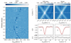 |
Fig. B.1. Cross-correlation functions of SVD detrended spectra. Left panel: As a function of the orbital phase (0 is the time of periastron) in the RG rest frame, with the MS companion clearly detected. Right upper panels: CCF maps from the K-focusing method. A 26.6-σ CCF signal marks the MS star’s orbit being aligned in the MS’s rest-frame. The best fitting Saltite model is used to measure the MS star semi-amplitude and rest-velocity. White lines (a & b) mark sections shown in the Right lower panels: Gray data points are CCF data, error bars represent the overall jitter from the two-dimensional fit. |
In a second step, we use the RV measurements to align all remaining 43 FIES spectra into the rest frame of the RG star. We then detrend (Sebastian et al. 2024a) the spectra by removing on average the first three components of a singular value decomposition (SVD, Kalman (1996)). This should effectively remove the lines of the RG star. The detrended spectra are then cross-correlated with a G9 line mask. Figure B.1 shows the CCF in the primaries rest frame. The trail of the MS star is clearly visible, as well as some residuals from the RG. These residuals are most likely caused by variations of the RG’s absorption spectrum during the ∼4.5 yr of observation. Systematic residuals from the RG were also found in the spectral separation performed in the main analysis, supporting the non-artefact origin. For the analysis of the companion, we therefore exclude all spectra where the radial velocity difference of both binary components is less than 20 km s−1. Since the companion signal is clearly visible in the CCF, we also identify three spectra which show very noisy CCF’s, and therefore exclude them from the analysis. For the 32 selected and detrended spectra, we use the K-focusing method to measure the MS companion semi-amplitude (Sebastian et al. 2024b). In this process, we keep the orbital parameters of the RG fixed and sample the MS semi-amplitude (K2) in steps of 1.5 km s−1 from 10 to 50 km s−1 and the companion rest velocity (Vrest, 2) in steps of 1.5 km s−1 from -130 to -70 km s−1. Figure B.1 shows the cross-correlation map of the companion, showing a 26.6-σ detection. We use the Saltire6 model to fit the map, which allows us to obtain precise parameter measurements of the MS orbit. The model assumes that the CCF of the MS companion follows a Gaussian shape, thus we can measure K2 and Vrest, 2, but also FWHM and relative CCF contrast of the companion’s mean line profile. To fit the data, we use a Markov Chain Monte Carlo (MCMC) implementation in Saltire to sample the posterior distribution for each of the fit parameters with 21,000 samples. The sections through the map in Figure B.1 show some deviations from this shape. The individual spectrum CCFs are also more noisy than the BF. This is likely due to the same as the K-focusing map sections: Additional statistical noise (the line mask is optimised for m/s exoplanet detection rather than S/N), the CCF has some minor peak-pulling behaviour and side-lobes compared with the BF, and the left-over spectrum has summed-up residuals from the SVD (Sebastian et al. 2024b) which are different from the non-SVD separation approach used in the main analysis. To measure the systematic uncertainties from this analysis, we split the data into 4 partial samples with four spectra each. We then repeat the analysis for each of them and adopt the RMS error as systematic uncertainty(Sebastian et al. 2024a), which we add to the fit uncertainties from the Saltire fit. The final results and uncertainties are reported in Table B.1.
The most important difference between the main RV analysis and this is on the semi-amplitude of the MS star, at 1.6σ. The S/N of the MS star in the spectra is very low, near ∼1 for the CCF analysis, and the detections are primarily noise-dominated, with some additional residuals from the SVD and CCF. As the BF analysis has a higher S/N detection for the MS star in all spectra, the difference of less than 2σ between two different methods, with completely different weighing of the data, can be reasonably argued as statistical. When performing a similar two-step analysis with the broadening function method and spectral separation following González & Levato (2006), by first fitting the RG individual RVs, and then fitting the MS orbital semi-amplitude with all other orbital elements fixed, we obtain KMS = 27.87 km/s, 0.5σ different from the main analysis and 1σ from the CCF analysis.
Appendix C: Spectroscopy, choice of line-list
The line-list used by the Gaia-ESO survey(Stetson & Pancino 2008) has a large number of blends and irregularly shaped lines for the RG. This is the reason we used the manually selected line-list given in Slumstrup et al. (2019). The line-list oscillator strengths of each absorption line has been calibrated on a solar spectrum obtained with the same spectrograph.
Spectroscopic atmospheric parameters, and abundances, for the RG in KIC 10001167, both ours (FIES) and from the APOGEE DR17 near-infrared survey.
For KIC 10001167, we perform separate spectral analysis using either the astrophysically calibrated oscillator strengths of Slumstrup et al. (2019), or the same lines but the laboratory values of Stetson & Pancino (2008).
With the internal uncertainties presented in Table C.1, the results using either are statistically consistent. We adopt only the astrophysically calibrated results based on the line-list of Slumstrup et al. (2019) for further analysis, since it has significantly higher internal precision, less tension between FeI and FeII, and an effective temperature compatible with the IRFM within 3 K (see Sect. F.3). For collective [Fe/H] we use only the [FeI/H] measurements, since the number of FeI lines far surpass the FeII lines, and because the FeII lines of KIC 10001167 are very weak and therefore sensitive to blending.
We also include effective temperature, metallicity and α enhancement from the APOGEE DR17 (Abdurro’uf et al. 2022), as it has infrared spectra available (apogee_id 2M19074937+4656118). We find that it is compatible with our analysis within the statistical uncertainties.
Results in Table C.1 have uncertainties calculated using a standard deviation of the lines, which reflect only line-to-line scatter and not systematic uncertainty. Therefore, for use in the rest of the analysis we follow the investigations of Bruntt et al. (2010) and adopt a total uncertainty of 0.1dex for [Fe/H] and [α/Fe].
Appendix D: Details on the binary analysis
D.1. JKTEBOP
To prepare the light curve for JKTEBOP analysis, low-order polynomial fitting of the data near the eclipses is performed to normalise each eclipse. The light curves are then truncated to keep a minimum amount of data outside of eclipses. Photometric uncertainty is estimated from the RMS of the phase-folded light curve within the total eclipse. This is the same procedure as (Thomsen et al. 2022), and ensures a homogeneous treatment of the eclipses after trends from reflection, deformation, beaming, and/or activity have been locally removed. Following this pre-processing, we disable the reflection and deformation approximations in JKTEBOP and treat the stars as spherical.
The PDCSAP light curve has lower apparent photometric noise than the other light-curves available to us, since it has been corrected for several known instrumental effects by the mission pipeline. We also have access to the KASOC light-curve (Handberg & Lund 2014) from the KASOC database7, and the Kepler mission pipeline SAP, which in this case has higher photometric noise but better retains out-of-eclipse trends from the binary orbit. We further verify that, after applying the same pre-processing to the KASOC (Handberg & Lund 2014) light curve and the Kepler pipeline SAP, we obtain best-fit results indistinguishable from our PDCSAP analysis. The KEPSEISMIC light curve is unsuitable for eclipse analysis, since it is heavily filtered.
We investigate the Kepler target pixel files with LIGHTKURVE (Lightkurve Collaboration 2018) and find no sources of contamination near KIC 10001167 with GaiaG magnitude below 17. Additionally, we find no significant in-system contamination in our investigations of potential spectroscopic contamination (Appendix E). We therefore treat contamination as negligible for both this, and the PHOEBE, eclipsing binary analysis.
In Fig. D.1, the best-fit JKTEBOP light curve model is compared to the Kepler PDCSAP light curve.
The limb darkening h1 and h2 coefficients are linearly interpolated from the tables of Claret & Southworth (2022) for the Kp bandpass, as this parameterisation has been found to be superior to other two-parameter limb darkening descriptions when fitting for one coefficient (Maxted 2023). Claret & Southworth (2022) used plane-parallel ATLAS atmosphere models (Castelli & Kurucz 2003). The limb darkening (h1, h2) parameterisation of the power-2 law is demonstrated below, as described in Southworth (2023):
 (D.1)
(D.1)
 (D.2)
(D.2)
 (D.3)
(D.3)
Here, F(μ) is the flux at position μ = cos γ along the stellar disk, γ is the angle from centre, F(1) refers to the central flux, and c and α are the two coefficients for the power law (Southworth 2023).
Similar to Thomsen et al. (2022), JKTEBOP was run iteratively to obtain the final limb darkening coefficients using dynamically derived log g’s and Teff for the main sequence star. In Appendix D.2, we test the effect of using different formulations of limb or gravity darkening when deriving the radius of the giant, and in Appendix D.3 we compare with a light curve model using PHOENIX (Husser et al. 2013) specific intensities, determining a systematic uncertainty of ∼0.7% for the radius of the RG.
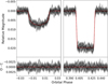 |
Fig. D.1. Eclipsing binary model fits with JKTEBOP to Kepler PDCSAP light curve for KIC 10001167. Observed-Calculated (O-C) residuals are shown below. |
Properties of KIC 10001167 obtained from eclipsing binary analysis.
D.2. Radius systematics, Gravity and Limb darkening prescription
Gravity darkening coefficients were fixed at 0.0 for both components during the main JKTEBOP analysis. Using gravity darkening coefficients from Claret & Bloemen (2011), we found no measurable differences in the parameters.
The limb darkening formulations described in this section can all be found in Southworth (2023). When using the re-parameterised power-2 limb darkening law, but h2 coefficient instead interpolated from the tables of Claret & Southworth (2023), which used spherical PHOENIX-COND atmosphere models (Husser et al. 2013) with solar abundances, the RG radius is increased by 0.2% (0.2σ). When using the four-parameter limb darkening law, and four coefficients fixed to interpolated values from Claret & Southworth (2023), the radius is lowered by 0.06% (0.07σ). We also tested several different two-parameter formulations keeping both coefficients fixed; 1. power-2 law with ATLAS-derived coefficients from Claret & Southworth (2022); 2. quadratic law with ATLAS-derived coefficients from Claret & Bloemen (2011); 3. quadratic law with ATLAS-derived coefficients from Sing (2010). The maximum deviation in RG radius, in-between these and when comparing each with the one with h1 free (and h2 from Claret & Southworth (2022)), was 0.3% (0.3σ). When increasing the effective temperature of the giant by 100K (and the MS star by 130K) while fitting h1, the measured radius decreased by 0.05% (0.05σ). When increasing the RG temperature by 200K (and MS by 260K) while fitting h1, the measured radius decreased by 0.09% (0.1σ). We note that the four-parameter law with pure-interpolated coefficients, which is the law best reproducing theoretical atmosphere models (Claret & Southworth 2023), produces a radius that is almost an exact match with our result determined using power-2 law with h1 free (deviation 0.06%), despite using a different atmosphere model (PHOENIX instead of ATLAS). In summary, the obtained radius is robust regardless of the exact limb darkening law used. Variations caused by the assumed limb darkening law (at maximum 0.3%) are insignificant compared with the uncertainty on the radius, which is ∼0.9%.
D.3. Radius systematics, Atmosphere and specific intensity
As implemented, all the limb darkening prescriptions tested in Sect. D.2 assume that the stellar atmosphere has a hard cut-off at the edge of the limb. This cut-off is taken as the point where the gradient of the specific intensity profile of the star is at maximum. We tested the validity of this approximation using the program ELLC (Maxted 2016), which allows for direct input of specific intensities. For the RG, we used specific intensities from PHOENIX-COND atmosphere models (Husser et al. 2013), interpolated to the effective temperature, metallicity and dynamical log g, and integrated over the Kepler passband. Then, we generated a synthetic light-curve with the complete set of specific intensities, and re-fitted the stellar radii, surface brightness ratio and inclination with a model using the aforementioned specific intensity cut-off. The re-fitted radii were ∼0.3% higher than the input radii. This demonstrates the direct influence that our assumption of a hard stellar surface has under perfect conditions.
After, we performed the same simulation, but for the re-fit model we utilised either the four-parameter limb darkening law with the same coefficients as Sect. D.2, or the power-2 law. In both cases, we find that the re-fitted RG radius decreases by 0.7% (and MS increases by 1.7%). It is also evident, from comparing the specific intensities, that both the limb darkening laws poorly reproduce the atmosphere model profile. We take the maximum deviation reported, from this and Sect D.2, as the combined systematic uncertainty on the dynamical radius of the RG.
D.4. Light travel time
In our JKTEBOP and PHOEBE analyses, light travel time effects have not been accounted for. The differential effect due to the orbit is negligible, but the constant system radial velocity has a significant effect on the perceived orbital period. We tested this with JKTEBOP by performing a linear correction of the time-stamps of all data (light-curve and radial velocities) using an approximate system velocity of −103 km/s, to account for the increasing distance between the target and the solar system. The measured orbital period is then decreased to 120.34868 days, a change of 0.03% (69σ). This decreases the orbital semi-major axis in turn by 0.03% (0.2σ), the mass of the RG by 0.03% (0.04σ), and the radius of the RG by 0.03% (0.04σ). Since the interest of the analysis is the fundamental stellar parameters, this effect can be safely ignored for KIC 10001167.
D.5. PHOEBE 2
For subsequent analysis with PHOEBE 2 (Conroy et al. 2020), we start from the unfiltered KASOC light curve. The PDCSAP light curve, while having lower noise due to the co-trending basis-vector corrections of the Kepler data analysis pipeline, suffers from over-fitting of the eclipsing binary signal from those same corrections. Since they are multiplicative, it is possible to correct for them by normalising the eclipses (as we have done and demonstrated in Appendix D.1). However, for PHOEBE we wish to model both the eclipses and out-of-eclipse signal of binarity, which makes the PDCSAP light curve unsuitable. The Kepler pipeline SAP light-curve would be a reasonable choice, but we decided to use the KASOC light curve, which is also based on simple aperture photometry, because it uses a larger aperture which reduces the impact of spacecraft motion on the light curve. We perform a custom, iterative filtering of the KASOC light curve, inspired by Handberg & Lund (2014). Here, we start with a window size much longer than the orbit for our non-phased long-trend filter, and incrementally reduce it as the transit is captured by a phase-folded filtering. This filtering is advantageous since it retains the complete (repeating) eclipsing binary signal both inside and outside of eclipses with limited over-fitting.
For the MCMC sampling with EMCEE, we use uninformative uniform priors around the JKTEBOP results, with boundaries at least four times the measured JKTEBOP uncertainties, and extend them if any parameter converged towards the edges.
The uncertainties we obtain from our MCMC sampling are heavily underestimated, and should not be used for comparing with other analyses. The sampling assumes that no residual signal remains in the light-curve besides the binary orbit signal, while the residuals for KIC 10001167 are clearly dominated by asteroseismic signal. We verify this by performing an independent MCMC sampling with the JKTEBOP light curve modelling and recovering similarly underestimated uncertainties. Due to computational expense, it is not possible to perform as detailed an investigation of the uncertainties as we perform with the JKTEBOP analysis. We therefore use the latter as the baseline result for comparison with asteroseismic, and photometric, inference.
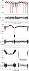 |
Fig. D.2. Eclipsing binary model fits with PHOEBE 2 to independently filtered KASOC light curve for KIC 10001167. Top panels illustrate the binned light curve (black points) and model (red) with time on the x-axis. Middle panels show the same, but with orbital phase on the x-axis. The bottom panels show zoomed-in views of just the two eclipses (phase-folded). The data have been binned in time, in three different ways depending on phase. See the text for details. The gaps between different binnings is a consequence of time-averaging within the bins, and a hard cut to avoid data overlap between them. |
Appendix E: Spectroscopic test for a potential unresolved third star
Using the FIES spectroscopy, we explored the possibility of stellar light contamination from an unresolved in-system third companion, to rule out biases on the dynamical RG radius therefrom. It was performed in a similar way to Brogaard et al. (2022). We subtract the separated component spectra from all observed spectra that have RVs for both the RG and the MS star, and then average them. Since the system velocity is found to be constant, a potential third stellar companion would have to be on a wide orbit and therefore have almost constant RV. If it is gravitationally bound, it should have low RV relative to the system. With the combined spectrum, we make a broadening function profile using the MS template spectrum. Here, we find no significant single peak, only spurious peaks 1.5 times the noise exactly within the ±25 km/s region, a clear leftover systematic from the RG spectral separation.
We then inject an artificial third star, by rotationally broadening the MS template with v sin i = 5 km/s, with noise calculated from the injection light ratio and the S/N of each spectrum. We adjust the light contribution from the third signal until the broadening function signal is 2 times the ±25km/s noise (3 times the noise outside), which occurs when the injected luminosity ratio is 0.5%. We set this as the detection threshold for a third companion. Assuming a luminosity of 70 L⊙ for the RG, this puts an upper limit of ∼ 0.35 L⊙ for an undetected third star. Statistically, such a star would be on the main sequence, meaning spectral type K3V or cooler8. It is unlikely that its brightness would be exactly at the detection limit. A contaminant with brightness far below the limit would not bias the light curve radius measurement.
Appendix F: Parallax, photometry, IRFM, and kinematics
Gaia Data Release 3 (DR3) offers parallax and photometry for KIC 10001167 (Gaia Collaboration 2016, 2023b). Table F.2 shows the astrometric parameters from Gaia DR3, including an additional uncertainty estimate due to the binary orbit, which we derive in Appendix F.1. Table F.1 includes photometric measurements of the RG derived using the DR3 parallax and either single-passband photometry with Gaia DR3 or 2MASS (Skrutskie et al. 2010) or the infra-red flux method (IRFM). It also includes MS star photometric contributions estimated in the IRFM using the eclipsing binary radius ratio (JKTEBOP) and effective temperature ratio (PHOEBE), in combination with DR3 photometry in the G, BP, and RP bands.
F.1. Parallax uncertainty
Assuming that the parallax-derived distance of Sect. F.4 is accurate, the orbital motion on the sky is expected to be significant in comparison to the parallax, with semi-major axis of 0.667 mas if the system is aligned for maximum movement on the sky. It could therefore bias the parallax measurement. We use the method mentioned in Brogaard et al. (2022) and detailed in Rappaport et al. (2022, Appendix C) to estimate an additional uncertainty contribution from this.
Summarising, we start by first assuming that the 35 astrometric transits are all instantaneously measured, and equi-spaced in time between the Gaia DR3 start and end dates of observation (2014/07/25 to 2017/05/28). To simplify the computation, we assume that the inclination is i = 90° such that the orbital movement happens only along a line on the sky, and we assume that the orbit is aligned for maximum variation on the sky. Then, we calculate the centre of light distance from the centre of mass using the eclipsing binary masses, luminosity ratio, semi-major axis, period, eccentricity, and periastron time. This is converted into a projected distance on the sky, in milli-arcseconds, for each simulated astrometric transit. From this, we calculate a standard deviation, and convert it into an approximate standard error by dividing with the square-root of the number of astrometric transits minus the number of astrometric fitting parameters (35-5). With this, we obtain a standard error of 0.040 mas, despite having a maximum orbital semi-major axis of 0.667 mas. These results, along with the Gaia DR3 astrometric parameters, can be found in Table F.2.
F.2. Extinction
We estimated the extinction using three different 3D dust maps: 1. BAYESTAR19, available through the python package DUSTMAPS (Green 2018; Green et al. 2019). 2. The map by Lallement (2019). 3. The updated map by Lallement et al. (2022).
The BAYESTAR19 map was converted to E(B-V) using the two example relations on their documentation website9 (either E(B-V) = 0.884 × (Bayestar19) or E(B-V) = 0.996×(Bayestar19). Then, they were converted to passband-specific extinction coefficients AX using the colour-relations of Casagrande et al. (2021, Table B1) (specifically, the EDR3 FSF relations). (BP-RP)0 was derived iteratively, starting with (BP-RP)-E(B-V) as initial guess.
From the Lallement (2019) and Lallement et al. (2022) maps, extinction at 550nm (A0) was obtained. To convert this to passband-specific extinction, we utilised the Gaia EDR3 auxiliary data files10. Here, we specifically made use of the (BP-RP) colour-relations for stars at the top of the HR diagram (Giants).
When we estimate extinction using the three different maps, while neglecting that KIC 10001167 is a binary, we find general agreement on a very low amount of extinction, but otherwise it is quite uncertain with E(B-V) between 0.03 and 0.04.
Due to this, for the IRFM and luminosity measurements we adopt a simple estimate of E(B−V) = 0.0350 ± 0.0105 which is in between the different measurements. Here, the uncertainty is conservatively taken as 30% of the value, which means that all three maps are well within 1σ. This large uncertainty ensures that we do not bias the final result due to selection of a specific map. At the same time however, since the reddening is small, it is not going to inflate the propagated uncertainties significantly.
IRFM measurements, photometry, and reddening of the stellar components in KIC 10001167, including magnitude corrections to account for the companion in the photometry.
F.3. Photometry and Infra-red Flux Method
We use the IRFM to simultaneously estimate the effective temperature and angular diameter of the RG. The IRFM implementation is described in Casagrande et al. (2021), which is based on Gaia and 2MASS photometry and has been extensively validated against interferometric and other benchmark stars. We fix [Fe/H]=−0.68 (APOGEE DR17), log g = 2.18 and E(B − V) = 0.035 (from Appendix F.2) to obtain an initial Teff = 4638 K and θ = 0.1379 mas for the RG. These values, together with the ratios of effective temperatures and radii from Table D.1, are used to correct Gaia and 2MASS photometry for the flux contribution of the MS star before running the IRFM again. We converge to Teff = 4625 K and θ = 0.1376 mas in one iteration, these values being identical regardless of adopting JKTEBOP or PHOEBE 2 ratios. Uncertainties in the flux contribution of the MS star are derived with 10,000 Monte Carlo realisations assuming normal errors for the effective temperature and radius ratios (Table D.1), metallicity (0.1 dex), gravity (0.1 dex), reddening (0.0105), 2 and 1 percent for the initial effective temperature and radius of the RG.
It can be appreciated from Table F.1 that the photometric contribution of the MS star is at most a few hundredths of a magnitude, with negligible uncertainties in all cases. To estimate final uncertainties on the effective temperature and angular size of the RG we run another 10,000 Monte Carlo realisations drawing again from a normal distribution in the adopted values of metallicity, reddening and photometry. These statistical uncertainties are provided in Table F.1 along with systematic ones for the IRFM and parallax. Systematic errors within the IRFM take into account the uncertainty of the zero point of the adopted Teff scale, inflated by a further 10K if we were to adopt a different reddening law (COD instead of FSF, see Casagrande et al. 2021, for further details).
Using the angular size of the RG with the Gaia DR3 distance measurement, we obtain a radius of 12.82 ± 0.30 (stat) ±0.24 (syst) R⊙. Combining effective temperature with photospheric radius, we measure a luminosity of 67.7 ± 6.1 L⊙. We report the IRFM results, along with single-passband bolometric luminosities assuming bolometric corrections from BOLOMETRIC-CORRECTIONS11 software (e.g. Casagrande & VandenBerg 2018, and references therein), in Table F.1. The bolometric corrections are based on MARCS model fluxes (Gustafsson et al. 2008), whereas the IRFM we describe in this section relies on model fluxes from Castelli & Kurucz (2003).
Table F.1 includes all the binary-corrected photometry, IRFM-based measurements, as well as luminosity and radius from single-passband measurements with all the Gaia DR3 and 2MASS passbands. The main contribution to the uncertainty in both approaches (IRFM vs. single-passband) is the parallax.
Astrometry and kinematics of KIC 10001167. See text for description.
F.4. Distance
The uncorrected parallax is 1.135 ± 0.018mas. The parallax error is increased using the re-scaling of the raw parallax error suggested by Maíz Apellániz et al. (2021), as well as with the additional parallax uncertainty estimate from the binary orbital motion that we find in Appendix F.1. The parallax zero-point is evaluated to be −0.019mas using the python package GAIADR3-ZEROPOINT (Lindegren 2021) and subsequently corrected for.
Excluding (including) the extra parallax uncertainty from the orbit, we measure a distance of  (
( ) pc when the parallax zero-point is corrected for. Without zero-point correction, we obtain 881pc. Both the geometric (866 ± 13pc) and photo-geometric (862 ± 11pc) distances from Bailer-Jones et al. (2021) are fully compatible with the zero-point corrected distance measurement we provide here. We propagate our additional uncertainty estimate from orbital motion for subsequent radius and luminosity inference. However, we use the final difference between the two uncertainty estimates as our reported systematic uncertainty estimate.
Appendix G: Asteroseismic details
G.1. MESA grid
The MESA (version n. 11701) grid used for asteroseismic inference spans a wide range of [Fe/H], [α/Fe] and helium abundance (Y) values. [Fe/H] ranges from -2.0 to 0.25 in steps of 0.25; Y ranges from 0.25 to 0.34 in steps of 0.03. We also consider four values of α-enhancement, [α/Fe]=-0.2,0.0,+0.2,+0.4. The reference solar mixture is the one from Asplund et al. (2009). For each choice of [Fe/H], Y and [α/Fe] values, we calculate models with masses between 0.6 and 1.8 M⊙, with a step of 0.05 M⊙. We adopt the atmosphere description by Krishna Swamy (1966) and other choices in terms of equation of state, opacities, and mixing are as in Miglio et al. (2021b). Finally, we use the mixing-length-theory (MLT) convection scheme in the formulation provided by Cox & Giuli (1968), where we set the αMLT parameter to 2.2902. This value is the result of a standard solar-model calibration process. Each model is evolved from the pre-main-sequence to the first thermal pulse. Adiabatic oscillation frequencies of angular degree l = 0 and 2 are computed using the code GYRE (Townsend & Teitler 2013, and references therein). For RGB stars with log10(⟨ρ⟩/ρcentre) larger than 8.0 we compute non-radial modes using the approximation presented in Ong & Basu (2020). As described by Tailo et al. (in preparation), this ensures that the frequencies of quadrupole p-dominated modes in RGB stars can be computed accurately (to better than 0.05% at L ∼ 65 L⊙) and in a computationally efficient manner. In low-mass stars, this threshold is met at L ≳ 30 L⊙, hence it is fully justified for KIC 10001167.
G.2. Frequency extraction
Fig. G.1 shows the agreement between all the observed frequencies of this work, as well as (Kallinger 2019). Table G.1 gives all frequencies observed by at least two pipelines.
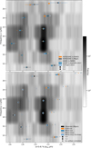 |
Fig. G.1. Echelle diagrams for the asteroseismology of KIC 10001167. X-axis shows frequency ν modulo 2.731 μHz (offset), and Y-axis shows frequency. Heat-map data is uniformly smoothed with window = 0.075μHz. Marker filling has been half/fully removed for some of the overlapping points. Top panel: l = 0 and l = 2 frequencies observed with five different methods described in Section 2.6.1. Only frequencies found with at least two methods are shown. Bottom panel: Best fit theoretical frequencies vs. a single set of observed frequencies (KEPSEISMIC+PBJam) that were used as observational constraints for the inference. |
Asteroseismic frequencies and average measures for the RG in KIC 10001167.
G.3. Individual mode frequency inference
We perform several runs of the AIMS code, changing either to the MESA model grid ([α/Fe] = 0.2), the CLÉS grid with [α/Fe] = 0.4, using luminosity instead of νmax, switching between the two metallicity and effective temperature sources, or using a different set of observed radial mode frequencies (KASOC+FAMED). These fits are illustrated in Figure G.2. We find that the inferred masses and radii are largely consistent across the runs, and we use this procedure to evaluate realistic systematic uncertainties on the quoted stellar parameters by taking, for each inferred parameter, the largest difference of the median between our reference run and all the aforementioned runs. The right-most run in Figure G.2 (MESA, helium free but constrained to > 0.248) is not taken into consideration for systematic uncertainty estimation, but will be compared with in the next paragraph.
Figure G.3 compares the CLÉS reference inference with three MESA inferences, all having the same source of asteroseismic (PBJam) and photospheric constraints (APOGEE DR17). The three MESA runs are; l = 0 modes and [α/Fe] = 0.2, l = 0 modes and [α/Fe] = 0.4, and finally l = 0,2 modes and [α/Fe] = 0.2 without fixing the initial helium fraction or using a helium enrichment law. Most importantly, changing the grid clearly has no significant effect on the inferred mass, and the age difference between the two can be associated with a difference in temperature scale. The initial helium mass fraction is not well-constrained, yet it is compatible with the expected close to primordial value. While some correlation is seen between mass and helium, the mass agrees to 1σ with the other results.
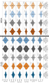 |
Fig. G.2. Violin plots of key stellar parameters for the 8 inferences used to define the asteroseismic measurement in Table 1, as well as for the helium-free inference (right-most). Left-most inference defines the reference for the median measurement and statistical uncertainty in Table 1, while the maximum median difference to the remaining 7 constrained-helium inferences defines the systematic uncertainty on the quoted parameters. See the Sect. 2.7 and Appendix G.3 for details. The median parameter values of the reference fit is drawn through the whole plot (grey dashed line). The helium-free inference here has a lower bound on initial helium of 0.248 corresponding to the primordial helium fraction. |
G.4. Asteroseismic mean density inversion
The consistency of the results provided from the fit of the radial modes was tested using a mean density inversion following Buldgen et al. (2019). To this end, we used the two sets of radial modes (KEPSEISMIC+FAMED, and KEPSEISMIC+PBJam) with respectively 5 and 6 individual modes and two reference models computed with CLÉS, and optimised with AIMS to reproduce the individual radial frequencies. To fully test the precision of the inversion, we also tested various surface corrections, namely that of Ball & Gizon (2014), that of Sonoi et al. (2015) and leaving no surface correction. The average of all these results provides a value of 6.39 ± 0.04 × 10⁻⁴ g/cm3 with two distinct families of solutions, one centred around 6.43 × 10⁻⁴g/cm3 when surface corrections are included, one centred around 6.35 × 10⁻⁴ g/cm3 without. This behaviour is typical of mean density inversions, where systematics will heavily dominate the total uncertainty budget. Ultimately, the inversion confirms the AIMS modelling which in retrospect is not surprising as AIMS succeeded in fitting the individual radial modes as primary data in the forward modelling procedure. In this particular case, no specific disagreement in mean density is observed.
G.5. Scaling relations
The asteroseismic scaling relations for mass and radius are given below (e.g. Sharma et al. 2016, and references therein):
 (G.1)
(G.1)
 (G.2)
(G.2)
Δν is the large frequency spacing in the asteroseismic power spectrum, and νmax is its frequency of maximum power. We use the solar reference values of Δν⊙ = 134.9μHz and νmax, ⊙ = 3090μHz following Handberg et al. (2017), and Teff, ⊙ = 5772K from IAU 2015 B3 (Prša et al. 2016).
The correction factor fΔν is a stellar modelling derived correction to account for the difference in internal structure between the RG and the Sun. When referring to the scaling relations in this work, we utilise the radial-mode-only Δν0 = 2.714 ± 0.017μHz, νmax = 19.784 ± 0.158μHz, fΔν from Rodrigues et al. (2017), and fνmax = 1.
Asteroseismic scaling relation measurements are provided in Table G.2. The corrected relations show an overall agreement with the individual frequency inference, but a 3.6% difference in average density (3σ), which is much smaller than the disagreement with eclipsing binary analysis. The mass obtained with the scaling relation is 0.970± 0.036 M⊙, which is 1σ consistent with the individual frequency inferences mainly due to the comparatively large statistical uncertainty. As these scalings are very sensitive to the assumptions surrounding measurement of νmax, Δν, and the model-inferred Δν correction, they can be systematically much more uncertain than the individual frequency inference. This is the reason that this work focuses on comparisons with the latter method for the purpose of ascertaining the accuracy of asteroseismic mass measurements.
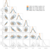 |
Fig. G.3. Corner plot showing a small selection of the asteroseismic inferences, all with the same Gaussian observational constraints highlighted by the full lines, ± the dotted lines indicating the 1σ level uncertainty on surface metal fraction, effective temperature, and frequency of maximum power. The grey MESA fit samples initial helium fraction as a free parameter. The lower bound on helium fraction is 0.248. The asteroseismic frequency constraints employed were KEPSEISMIC+PBJam (see Sect. 2.6.1 for description). |
Asteroseismic and dynamical measurements of the RG in KIC 10001167.
Appendix H: Evolutionary stage of the RG
We attempted, with well-established methods (Mosser et al. 2012), to measure an asymptotic period spacing from the dipole modes of the RG, and found that we were unable to clearly resolve any mixed dipole modes. If the RG had been core-Helium burning, this should have been straightforward as the period spacing would take on large values causing very well-separated mixed modes (see e.g. Mosser et al. 2012, 2014). This is what we furthermore demonstrate with synthetic asteroseismic spectra in Fig. H.1, and we detail their calculation below.
We also attempted an asteroseismic inference assuming that the RG is past the RGB, and fitted the radial modes only. The best-fit obtained this way is found at the very end of the red clump (RC), while a small fraction of He is still being burned in the core. With this fit, the surface correction coefficients take on nonphysical values, giving it the appearance of a linear frequency shift rather than an asymptotic behaviour towards lower frequencies. The temperature recovered with this fit is more than 200K higher than observed.
Fig. H.1 compares the observed power spectrum with simulated asteroseismic power spectral densities calculated with the code AADG V3.0.2 (AsteroFLAG Artificial Dataset Generator, Ball et al. 2018), one for a late-RC/early-Asymptotic Giant Branch (AGB) similar to the radial mode only post-RGB solution described above, and one for the RGB. These power spectral densities simulate 4-year-long Kepler observations of a red-giant star with M = 0.95 M⊙, [Fe/H] = −0.75 and [α/ Fe] = 0.4, with νmax and Δν approximately equivalent to the observed values; we adopted the values of the radial mode line-widths observed in large samples of RGB and early-AGB stars (Vrard et al. 2018; Dréau et al. 2021) in these simulations (i.e. similarly to Matteuzzi et al. 2023). These clearly show that the RGB phase is the most credible phase for KIC 10001167, since the observed mixed-mode behaviour of the dipole (ℓ = 1) modes is only compatible with the RGB simulation.
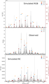 |
Fig. H.1. Top panel: Simulated power spectral density (PSD) for RGB star. Middle panel: Observed PSD, divided by granulation background. Bottom panel: Simulated PSD for a late-clump/early AGB star. For the simulated PSD, the mixed ℓ = 1 modes are highlighted, with an amplitude proxy calculated from the mode inertia and a Gaussian envelope. |
H.1. Further evolutionary considerations from population membership and binary orbit
The kinematics, metallicity, and α-enhancement points towards KIC 10001167 being a member of the old, thick disk population of the Milky Way. If the RG has evolved past the RGB through single-star evolution, it would have gone through the He flash and lost a significant amount of mass. Its initial mass would be much higher, and therefore the system should then be younger than what is compatible with the rest of the old disk population.
The RG currently has a radius of about ∼10% the size of the semi-major axis (13.03 R⊙ vs. 124.17 R⊙). From stellar models, the RGB tip radius of a star with this mass is expected to be ∼ 120 R⊙. Given the current orbital separation and eccentricity, if the star had evolved past the tip its companion must have entered the convective envelope at that point during its evolution. It is unlikely that the binary would have survived this, further demonstrating that the RG must be on the RGB.
Appendix I: Influence of tides on the RG
As shown in Fig. D.2, the light curve has a clear tidal deformation signal from the RG in KIC 1001167. However, this still amounts to only a small level of deformation from spherical. When assuming the stellar shape as a bi-axial ellipsoid, the approximated oblateness (a − b)/a is less than 0.002. This means that, for all intents and purposes besides fitting the filtered light curve, the star can be assumed spherical.
Beck et al. (2024) suggests that radius expansion, caused by tidal interaction with a companion, could lead to overestimation of the seismically inferred mass and radius. So far, this claim does not seem to have been tested. The assumption underlying this is that there should be a natural change in internal structure profile due to interaction with the companion, in a way that perturbs the seismic profile significantly from what can be predicted using traditional stellar modelling.
KIC 10001167 is not in a regime where detailed investigation is relevant. The level of tidal apsidal motion is expected to be very small at its current evolutionary state, and we have not been able to fit a significant linear apsidal motion to the light curve and radial velocities. Angular momentum transfer between the RG internals and the binary orbit is therefore currently below detectable levels, indicating that the tidal displacement of matter is still low despite showing significant flux variation. Additionally, we have performed two tests using representative stellar evolutionary tracks calculated with MESA. Both have [Fe/H]=-0.75, [α/Fe] = 0.4, Y = 0.25, with either initial mass 0.90 M⊙ or 0.95 M⊙. We calculated the circularisation function from Beck et al. (2024, eq. 7) by integrating numerically from zero-age main sequence up to the age where the radius of the star surpasses 13.03 R⊙. With this, we obtain a rate of eccentricity reduction of ϵr = −0.37 for initial mass 0.90 M⊙ and ϵr = −0.42 for 0.95 M⊙ (using Beck et al. 2024, eq. 5, eq. 6). This is significantly below the critical ϵcrit = 0.478 which is suggested by Verbunt & Phinney (1995) to separate systems with strong and weak tides. This demonstrates that tidal history is not a likely explanation for the differences we see between asteroseismology and eclipsing binary measurements of KIC 10001167.
Appendix J: Mass-loss on the RGB
Our stellar models do not include mass loss during the RGB, which does not impact our main findings, meaning our tests on the mass recovery of asteroseismology. If mass loss is included in stellar models, it is typically through simple analytic mass loss prescriptions (e.g. Reimers 1975). In reality, the exact occurrence of mass loss during the RGB has not been observationally established, rather, integrated mass loss from RGB to red clump is better quantified (see e.g. Brogaard et al. 2024). If we assume the Reimers (1975) prescription, the integrated RGB–RC mass loss measurements of Brogaard et al. (2024) would indicate η ∼ 0.4 for a star with the properties of KIC 10001167. With η = 0.2, 0.4, 0.6, we can predict that the RG should then have lost 0.6, 1.2, 1.8% of its mass, respectively. Ignoring it demonstrates a potential systematic uncertainty on the age of 2, 4, 6% for this star depending on adopted η. All these estimates are roughly equivalent to or below our adopted systematic uncertainty. We stress again that there is currently no observational indication of significant mass loss at luminosities comparable to that of this object.
Appendix K: All radial velocity measurements
Table detailing the spectroscopic radial velocity follow-up observations for KIC 10001167.
All Tables
Spectroscopic atmospheric parameters, and abundances, for the RG in KIC 10001167, both ours (FIES) and from the APOGEE DR17 near-infrared survey.
IRFM measurements, photometry, and reddening of the stellar components in KIC 10001167, including magnitude corrections to account for the companion in the photometry.
Table detailing the spectroscopic radial velocity follow-up observations for KIC 10001167.
All Figures
|
Fig. 1. α-enhancement level vs. iron abundance from APOGEE DR17 for stars with 1.5 < log g < 3. KIC 10001167 is highlighted. |
| In the text | |
|
Fig. 2. Top: Binary signal in the light curve, along with the best-fit PHOEBE 2 model. Bottom: RV measurements and dynamical RV curves for the two stellar components. The dotted vertical lines indicate the location of eclipses. Both top and bottom panels include O-C residual sub-panels. |
| In the text | |
|
Fig. 3. Top: Frequency-power spectrum divided by the granulation background in the original (light) and uniformly smoothed (dark, window = 0.15 μHz). The vertical lines highlight the observed radial (ℓ = 0), dipole (ℓ = 1), and quadrupole (ℓ = 2) modes. Middle: Échelle diagram. The axes are flipped for illustration, showing observed radial ℓ = 0 and quadrupole ℓ = 2 frequencies and the best-fit frequencies from our reference radial mode fit. The heat-map data were uniformly smoothed with a window = 0.075 μHz. Bottom: Statistical significance of the O-C residuals relative to the measurement uncertainty σ. The marker-size was rescaled (in log10) to demonstrate the statistical weight 1/σ2 applied to each observed frequency in the asteroseismic inference. |
| In the text | |
|
Fig. 4. Top: Hertzsprung-Russell diagram with the luminosity of the RG and MS from the eclipsing binary radius and the IRFM temperature (this work). The two isochrones shown were calculated from the MESA grid of stellar models used in this paper. We also include eclipsing binary measurements from Gaulme et al. (2016) and the asteroseismic inference of the RG from Montalbán et al. (2021). Bottom: Mass and radius of the same sources, along with the same isochrones. All markers have error bars in x and y, but in some cases, they are smaller than the marker. |
| In the text | |
|
Fig. 5. Top: RG mass vs. radius measurements from this work and from the literature. The contours represent one and two sigma. As guides, circles are drawn around our eclipsing binary measurement representing a 2 and 5% radial difference in mass and radius. The arrow represents ±1σ for the radius measurement with the infrared flux method and Gaia DR3 parallax. Bottom: Mass vs. age from the stellar model inferences. |
| In the text | |
|
Fig. B.1. Cross-correlation functions of SVD detrended spectra. Left panel: As a function of the orbital phase (0 is the time of periastron) in the RG rest frame, with the MS companion clearly detected. Right upper panels: CCF maps from the K-focusing method. A 26.6-σ CCF signal marks the MS star’s orbit being aligned in the MS’s rest-frame. The best fitting Saltite model is used to measure the MS star semi-amplitude and rest-velocity. White lines (a & b) mark sections shown in the Right lower panels: Gray data points are CCF data, error bars represent the overall jitter from the two-dimensional fit. |
| In the text | |
|
Fig. D.1. Eclipsing binary model fits with JKTEBOP to Kepler PDCSAP light curve for KIC 10001167. Observed-Calculated (O-C) residuals are shown below. |
| In the text | |
|
Fig. D.2. Eclipsing binary model fits with PHOEBE 2 to independently filtered KASOC light curve for KIC 10001167. Top panels illustrate the binned light curve (black points) and model (red) with time on the x-axis. Middle panels show the same, but with orbital phase on the x-axis. The bottom panels show zoomed-in views of just the two eclipses (phase-folded). The data have been binned in time, in three different ways depending on phase. See the text for details. The gaps between different binnings is a consequence of time-averaging within the bins, and a hard cut to avoid data overlap between them. |
| In the text | |
|
Fig. G.1. Echelle diagrams for the asteroseismology of KIC 10001167. X-axis shows frequency ν modulo 2.731 μHz (offset), and Y-axis shows frequency. Heat-map data is uniformly smoothed with window = 0.075μHz. Marker filling has been half/fully removed for some of the overlapping points. Top panel: l = 0 and l = 2 frequencies observed with five different methods described in Section 2.6.1. Only frequencies found with at least two methods are shown. Bottom panel: Best fit theoretical frequencies vs. a single set of observed frequencies (KEPSEISMIC+PBJam) that were used as observational constraints for the inference. |
| In the text | |
|
Fig. G.2. Violin plots of key stellar parameters for the 8 inferences used to define the asteroseismic measurement in Table 1, as well as for the helium-free inference (right-most). Left-most inference defines the reference for the median measurement and statistical uncertainty in Table 1, while the maximum median difference to the remaining 7 constrained-helium inferences defines the systematic uncertainty on the quoted parameters. See the Sect. 2.7 and Appendix G.3 for details. The median parameter values of the reference fit is drawn through the whole plot (grey dashed line). The helium-free inference here has a lower bound on initial helium of 0.248 corresponding to the primordial helium fraction. |
| In the text | |
|
Fig. G.3. Corner plot showing a small selection of the asteroseismic inferences, all with the same Gaussian observational constraints highlighted by the full lines, ± the dotted lines indicating the 1σ level uncertainty on surface metal fraction, effective temperature, and frequency of maximum power. The grey MESA fit samples initial helium fraction as a free parameter. The lower bound on helium fraction is 0.248. The asteroseismic frequency constraints employed were KEPSEISMIC+PBJam (see Sect. 2.6.1 for description). |
| In the text | |
|
Fig. H.1. Top panel: Simulated power spectral density (PSD) for RGB star. Middle panel: Observed PSD, divided by granulation background. Bottom panel: Simulated PSD for a late-clump/early AGB star. For the simulated PSD, the mixed ℓ = 1 modes are highlighted, with an amplitude proxy calculated from the mode inertia and a Gaussian envelope. |
| In the text | |
Current usage metrics show cumulative count of Article Views (full-text article views including HTML views, PDF and ePub downloads, according to the available data) and Abstracts Views on Vision4Press platform.
Data correspond to usage on the plateform after 2015. The current usage metrics is available 48-96 hours after online publication and is updated daily on week days.
Initial download of the metrics may take a while.