| Issue |
A&A
Volume 696, April 2025
|
|
|---|---|---|
| Article Number | A42 | |
| Number of page(s) | 17 | |
| Section | Stellar structure and evolution | |
| DOI | https://doi.org/10.1051/0004-6361/202452626 | |
| Published online | 08 April 2025 | |
Improving the stellar age determination through joint modeling of binarity and asteroseismology
Grid modeling of the seismic red giant binary KIC 9163796
1
Instituto de Astrofísica de Canarias, E-38200 La Laguna, Tenerife, Spain
2
Departamento de Astrofísica, Universidad de La Laguna, E-38206 La Laguna, Tenerife, Spain
3
Max-Planck-Institut für Astrophysik, Karl-Schwarzschild-Straße 1, 85741 Garching bei München, Germany
4
Department of Astrophysics, IMAPP, Radboud University Nijmegen, PO Box 9010 6500 GL Nijmegen, The Netherlands
5
Institute of Astronomy, KU Leuven, Celestijnenlaan 200D, 3001 Leuven, Belgium
6
Department of Physics and Astronomy, California State University, Long Beach, Long Beach, CA 90840, USA
7
INAF – Osservatorio Astronomico d’Abruzzo, Via M. Maggini sn., Teramo, Abruzzo, Italy
8
INFN – Sezione di Pisa, Largo Pontecorvo 3, 56127 Pisa, Italy
9
Université Paris-Saclay, Université Paris Cité, CEA, CNRS, AIM, 91191 Gif-sur-Yvette, France
10
Institut für Physik, Karl-Franzens Universität Graz, Universitätsplatz 5/II, NAWI Graz, 8010 Graz, Austria
11
Sydney Institute for Astronomy (SIfA), School of Physics, University of Sydney, NSW 2006, Australia
12
Graz University of Technology, Rechbauerstraße 12, Graz, Austria
13
School of Physics, University of New South Wales, Sydney NSW 2052, Australia
⋆ Corresponding author; This email address is being protected from spambots. You need JavaScript enabled to view it.
Received:
15
October
2024
Accepted:
14
January
2025
Abstract
Context. The typical uncertainties of ages determined for single star giants from isochrone fitting using single-epoch spectroscopy and photometry without any additional constraints are 30–50%. Binary systems, particularly double-lined spectroscopic binaries, provide an opportunity to study the intricacies of internal stellar physics and better determine stellar parameters, particularly stellar age.
Aims. By using the constraints from binarity and asteroseismology, we aim to obtain precise age and stellar parameters for the red giant-subgiant binary system KIC 9163796, a system with a mass ratio of 1.015 but distinctly different positions in the Hertzsprung–Russell diagram.
Methods. We computed a multidimensional model grid of individual stellar models. From different combinations of figures of merit, we used the constraints drawn from binarity, spectroscopy, and asteroseismology to determine the stellar mass, chemical composition, and age of KIC 9163796.
Results. Our combined-modeling approach leads to an age estimation of the binary system KIC 9163796 of 2.44−0.20+0.25 Gyr, which corresponds to a relative error in the age of 9%. Furthermore, we found both components exhibit an equal initial helium abundance of 0.27 to 0.30, which is significantly higher than the primordial helium abundance, and an initial heavy metal abundance below the spectroscopic value. The masses from our models are in agreement with the masses derived from the asteroseismic scaling relations.
Conclusions. By exploiting the distinct positions of the components of KIC 9163796, we successfully demonstrate that combining asteroseismic and binary constraints leads to a significant improvement in the precision of age estimation, resulting in a relative error in age below 10% for a giant star.
Key words: asteroseismology / binaries: spectroscopic / stars: late-type / stars: oscillations / stars: individual: KIC 9163796
© The Authors 2025
 Open Access article, published by EDP Sciences, under the terms of the Creative Commons Attribution License (https://creativecommons.org/licenses/by/4.0), which permits unrestricted use, distribution, and reproduction in any medium, provided the original work is properly cited.
This article is published in open access under the Subscribe to Open model. This email address is being protected from spambots. You need JavaScript enabled to view it. to support open access publication.
1. Introduction
Knowing the precise ages of stars is crucial for many fields of astrophysics (Soderblom 2010), particularly in Galactic archaeology (Freeman & Bland-Hawthorn 2002) and stellar population studies (Wang et al. 2024). A commonly used technique for stellar age determination is isochrone fitting. However, it only applies with reasonable precision to stars close to the subgiant turnoff but can show large uncertainties for main-sequence field stars (Valle et al. 2013; Lebreton & Goupil 2014; Godoy-Rivera et al. 2021). For red giants, this method delivers relative age uncertainties of 30–50% (Casagrande et al. 2016). In the past decade, with the advent of space missions such as NASA’s Kepler (Borucki et al. 2010) and the Transiting Exoplanet Survey Satellite (TESS; Ricker et al. 2014), asteroseismology has gained significance as a tool for determining different parameters such as age for different types of stars but for red giant branch (RGB) stars in particular (e.g., Li et al. 2022; Warfield et al. 2024). Generally, two approaches for asteroseismic age determination exist: modeling using the frequency of maximum oscillation power νmax and the large frequency separation Δν (i.e., the global seismic parameters; e.g., Valle et al. 2015; Casagrande et al. 2016; Pinsonneault et al. 2018) and boutique modeling of oscillation modes (e.g., Lebreton & Goupil 2014; Campante et al. 2023; Li et al. 2024). While the latter can deliver precise results for certain targets, calculating comprehensive frequency grids for post-main-sequence stars, particularly RGB and red-clump stars, is very resource intensive, and the modes from models are susceptible to poorly modeled surface effects, particularly in active stars (e.g., García et al. 2014a; Salabert et al. 2016). Ages from modeling using the global seismic parameters can be especially powerful if combined with additional constraints, as in the case of globular clusters (e.g., Moser et al. 2023; Howell et al. 2024), open clusters (Brogaard et al. 2023), or binary systems (Johnston et al. 2019a; Murphy et al. 2021).
Depending on the spectral type and age, estimations are that 50% to 100% of stars are in binary systems (e.g., Raghavan et al. 2010; Moe & Di Stefano 2017; Badenes et al. 2018; Offner et al. 2023, and references therein). Unless the binary system was created from a very rare capturing event, the components of binary systems were born in the same cloud at the same time (e.g., Prša 2018; Moe & Di Stefano 2017). Therefore, they exhibit identical initial conditions, such as initial chemical abundances, ages, and distance to the observer. These binary constraints enable the use of such coeval systems as test beds for stellar physics and evolution (e.g., Cassisi & Salaris 2011; del Burgo & Allende Prieto 2018; Valle et al. 2018, 2023; Johnston et al. 2019b; Murphy et al. 2021). Especially powerful is a binary system where at least one of its components exhibits solar-like oscillations. Until recently, only around 100 of such unique systems were known (Beck et al. 2022). It was only the third data release (DR3; Gaia Collaboration 2023a) of the ESA Gaia mission (Gaia Collaboration 2016), which included a dedicated non-single star catalog for the first time, that made it possible to increase the number of known oscillating binary systems up to 1000 (Beck et al. 2024). However, only a handful red giant systems with both components exhibiting a power excess have been studied (Rawls et al. 2016; Beck et al. 2018). One of these previously studied systems is KIC 9163796, a double-lined spectroscopic binary system (SB2) composed of an RGB star and a subgiant star, that has been described observationally in detail by Beck et al. (2018, hereafter BKP18). Detections of oscillations in both components from Kepler light curves combined with its SB2 nature enabled BKP18 to give masses and radii for both components. Given its binary nature, the differences in the observational parameters for the two stars, described in detail in Sect. 2, are solely caused by the difference in mass between the components of 1.5 ± 0.5% (BKP18). This mass difference also causes the two components to be in distinct and favorable positions on the Hertzsprung-Russel diagram (HRD), as shown in Fig. 1. The primary is moving up the RGB and is strongly affected by changes in the mixing length parameter in modeling while exhibiting small fractional changes in effective temperature. In contrast, the subgiant exhibits large fractional changes in effective temperature per unit time as it moves horizontally in very short timescales in the HRD. Due to its observations with spectroscopy, asteroseismology, and binarity and the distinct positions of the components in the HRD (Fig. 1), KIC 9163796 enables degeneracies to be broken, such as the mass-initial helium degeneration, and allows a precise age estimation of the system to be obtained.
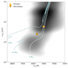 |
Fig. 1. Hertzsprung-Russel diagram depicting the positions of the primary (upward triangle) and secondary (downward triangle) component of KIC 9163796 according to the asteroseismic analysis from Beck et al. (2018). As references, the tracks of a 1 M⊙, 1.4 M⊙, and 2 M⊙ evolutionary track with the primary’s metallicity from MESA are provided as dashed lines. The background contour plot shows the density distribution of all targets from the input catalogs used in Beck et al. (2024), Mathur et al. (2022) with an asteroseismic detection. |
In this work, we present an asteroseismic grid modeling and age determination of the binary system KIC 9163796 by combining models from stellar evolution and oscillation codes with observational constraints from spectroscopy, asteroseismology, and binarity. The paper is structured as follows. In Sect. 2, we provide an overview of the observational constraints of KIC 9163796 in the literature that are relevant for the modeling. Section 3 explains how the model grid was obtained, while Sect. 4 describes the figure of merit and error estimation used for modeling. In Sect. 5, we describe the search for the best-fitting model combinations for the different cases of the figure of merit and different constraints from binarity. In Section 6, we discuss the results from this grid modeling approach, and we conclude in Sect. 7.
2. Observational constraints of the system
KIC 91637961 was shown by Beck et al. (2014) to be an oscillating red giant subgiant binary located in an eccentric orbit (e = 0.69 ± 0.01) with an orbital period of Porb = 121.30 ± 0.01 d. The system was initially detected in Kepler photometry due to a periodic flux variation induced by tides during periastron passage in a highly eccentric orbit (Zahn 1975; Remus et al. 2012). Due to the resemblance of echo-cardiograms in their lightcurve Thompson et al. (2012) coined the phrase ’heartbeat stars’ for this class of eccentric binaries (Kumar et al. 1995; Welsh et al. 2011).
The original analysis by Beck et al. (2014) revealed solar-like oscillations with relatively low amplitudes compared to similar red giants within the bulk asteroseismic sample (e.g., Kallinger et al. 2014). In a detailed study of the system, BKP18 presented a revised asteroseismic analysis based on the ∼1400 days long of the Kepler light curve (Kepler Quarters 0-14). The seismic analysis was done on the KEPSEISMIC2 data (for details of the database and calibration see García et al. 2011, 2014b; Pires et al. 2015). By re-evaluating the seismic parameters and spectroscopic parameters from Beck et al. 2014 (Revised values: νmax = 165.3 ± 1.3 μ Hz; Δν = 12.83 ±0.03 μ Hz; Teff = 5020 K), BKP18 determined a revised estimate for the seismic mass and radius for the primary M1 = 1.39 ± 0.06 M⊙ and R1 = 5.35 ± 0.09 R⊙. Using the asymptotic period spacing of the dipole mixed modes of ΔΠ1 = 80.78 s, BKP18 determined the evolutionary state of the primary to be located on the RGB, which corresponds to the H-shell burning phase. Within the uncertainties, the global asteroseismic values of the primary from BKP18 are in agreement with the recent values from the APOKASC-3 catalog (Pinsonneault et al. 2025).
From time series spectroscopy, obtained with the High-Efficiency and High-Resolution Mercator Echelle Spectrograph (HERMES, Raskin et al. 2011), BKP18 found KIC 9163796 to be a double-lined spectroscopic binary (SB2). From disentangling the composite spectrum in Fourier space (Ilijic et al. 2004), BKP18 found the mass ratio to be q = M1/M2 = 1.015 ± 0.005. As expected for a binary born from the same cloud, the metallicity for the primary and secondary agree within the uncertainties ([M/H]1 = −0.37 ± 0.1 dex and [M/H]2 = −0.38 ± 0.1 dex, respectively; with a reference solar iron abundance of Z⊙ = 0.0134). Despite their similarities in mass and metallicity, other fundamental parameters of the two components differ significantly, Teff, 1 = 5020 ± 100 K vs. Teff, 2 = 5650 ± 70 K, and log g1 = 3.14 ± 0.2 dex vs. log g2 = 3.48 ± 0.3 dex. From spectroscopy, BKP18 determined that the primary and secondary contribute 60% and 40% to the total flux, respectively. Due to the photometric dilution of the flux from each component, the relative flux variations of the oscillation modes are reduced by the same fraction. However, we do not expect the flux dilution to impact the extracted seismic parameters (e.g., Sekaran et al. 2019). Figure 1 depicts the positions of the components in the asteroseismic HRD.
While the power excess of the secondary was found at 215 ± 4 μ Hz, it was shown to be the reflection of the actual power excess at νmax, 2 = 340 ± 20 μ Hz, located above the Nyquist frequency of 283 μ Hz for the ∼30 minute long-cadence data of Kepler. Because of the low signal-to-noise ratio (S/N) of the secondary’s oscillation modes and the overlap with the primary’s power excess, no value for the large frequency separation could be determined. From the position of the power excess, the He-core of the secondary is already degenerated. BKP18 therefore considered the secondary an early RGB star too. Other criteria, based on the position of the secondary in the HRD shown in Fig. 1, classifies the star as a late subgiant (e.g., Godoy-Rivera et al. 2025).
Another notable difference between the two components is their photospheric abundance of lithium. From the disentangled HERMES spectra, BKP18 determined a lithium abundance for the primary of 1.31 ± 0.08 dex and the secondary 2.55 ± 0.07 dex, differing by a factor of 17. BKP18 could only explain this observational difference, with both components being in a particular short-lived state of stellar evolution, the first dredge-up (FDU). During this brief phase of stellar evolution, located near the beginning of the RGB, the convective envelope deepens into the stellar interior. It causes the mixing of the material produced from hydrogen burning during the main sequence. This mixing causes a depletion of the lithium abundance, and a change in the carbon isotopes ratio and nitrogen abundance at the surface during the FDU (Roberts et al. 2024, and references therein). Therefore, BKP18 concluded that the secondary component of KIC 9163796, which is richer in lithium than the primary, is in the early phase of the FDU. In contrast, the more massive primary evolved faster and is in a more advanced state of the FDU, causing a more effective mixing and lithium depletion.
For this paper, we reanalyzed the disentangled HERMES spectra assuming the same parameters as BKP18 to determine the α-element abundances. The measurement has been made with the BACCHUS code (Masseron et al. 2016) which includes MARCS model atmospheres (Gustafsson et al. 2008) and linelists from Heiter et al. (2015). This analysis indicated no enhancement nor depletion of Mg, Si, or Ca, and provided an α-element abundances of [α/Fe] = 0.0 ± 0.1 dex for both components.
Since the analysis by Beck et al. (2014) and BKP18, the ESA Gaia (Gaia Collaboration 2016) mission has included KIC 9163796 in all three data releases. In the latest Gaia DR3 (Gaia Collaboration 2023a) KIC 9163796 has an apparent G mean combined magnitude of 9.6 mag that have a color index GBP − GRP = 0.60 mag. The measured parallax is 2.23 mas, corresponding to a target distance of about 445 pc. The system is not listed in the non-single star catalog of Gaia DR3 (Gaia Collaboration 2023b). The target renormalized unit weight error (ruwe) value, an indicator for the object to be a single star (ruwe ∼ 1) or potentially non-single star (ruwe > 1.4), is given as 1.051. Beck et al. (2024) has shown that a significant percentage of known binaries (around 40 % in their sample) exhibit a ruwe below the generally accepted threshold of 1.4. Furthermore, neither multi-epoch photometry nor radial velocity was measured by Gaia for this object.
A direct estimate of the distance of KIC 9163796 as the inverse of the parallax from DR3 (ϖ = 2.23 ± 0.01 mas) results in a distance of d = 448 ± 5 pc. This is in agreement with the distances of  pc, that is determined by the General Stellar Parametrizer from Photometry (GSP-Phot, Andrae et al. 2023), which assumes a single star solution. A distance modulus estimate from the asteroseismic luminosity and apparent magnitude values in BKP18 results in a distance of ∼400 pc. However, it disagrees by more than 2-σ with the multi-star classifier (MSC)3 distance (d =
  pc), which assumes an unresolved binary solution (as is the case for KIC 9163796). Ulla et al. (2022) suggests that for some cases of unresolved binaries, the single-star solution of the GSP-Phot solution might be in better agreement with independent measurements compared to the MSC distance. The distance modulus solution and median photogeometric distance (dmed = 445 pc) from Bailer-Jones et al. (2021) point in the same direction, so we decide to trust the value inferred from GSP-Phot of d =
  pc as the reference for the distance to KIC 9163796. Table 1 summarizes all observables relevant for this work.
Observational parameters of KIC 9163796.
3. Constructing the model grid
To model KIC 9163796, we used the 1D-stellar evolutionary code MESA (Modules for Experiments in Stellar Astrophysics; Paxton et al. 2011, 2013, 2015, 2018, 2019; Jermyn et al. 2023, version r23.05.1) and the stellar oscillations code GYRE (Townsend & Teitler 2013, version 7.1) in a combined grid modeling approach. Using MESA, we calculated a grid of single-star models to search for the best combination of models for the primary and secondary under the constraints imposed by the common age (Age1 = Age2) and chemical composition. For the grid of models, we varied the stellar mass M, metallicity Z, and helium abundances Y in the ranges and stepsizes given in Table 2. Regarding the heavy element distribution adopted in the stellar modeling, we rely on a solar-scaled mixture (Grevesse & Sauval 1998). This choice is fully supported by the reanalysis of the spectra (Sect. 2) that shows that our stellar target does not show any evidence of α-element enhancement.
Parameter range for the model grid used in this work.
For the stellar mass range of the grid, we chose an interval centered on the mass of the primary reported by BKP18 from an asteroseismic analysis and extended three times the reported uncertainty toward higher and lower masses. This resulted in a lower limit of 1.22 M⊙ and an upper limit of 1.54 M⊙. To account for the lower mass of the secondary of 1.37 M⊙, we set the lower limit to 1.20 M⊙. With ∼1% being the lowest feasible observational uncertainty for stellar mass, we choose a stepsize of 0.01 M⊙.
We followed a similar approach for the initial metallicity, creating a grid range of two times the uncertainty centered on the spectroscopic value of the metallicity. This resulted in a range of −0.57 dex to −0.17 dex. Prior to modeling the with MESA, we converted the spectroscopic metallicity into the fractional mass component using the following equation:
![Mathematical equation: $$ \begin{aligned} Z_{\star } \sim Z_{\odot } \times 10^{[M/H]}\,{.} \end{aligned} $$](/articles/aa/full_html/2025/04/aa52626-24/aa52626-24-eq5.gif) (1)
(1)
When assuming the solar iron abundance value used for the spectroscopic analysis in BKP18 (Sect. 2), the heavy element abundance of the primary of [M/H] = −0.37 dex translates into Zspec = 0.006. Correspondingly, the upper and lower boundaries of our modeling result in Zlow = 0.004 and Zhigh = 0.010. As a stepsize, we decided to use 0.001, as translated in logarithmic space, this is approximately the order of the lowest feasible observational uncertainty.
For the initial helium abundance, which was added as a free parameter to account for a potential mass-initial helium degeneracy (e.g., Valle et al. 2014; Verma et al. 2022, and references therein), we chose a range similar to the one used in Lebreton & Goupil (2014), who did a similar modeling for a single star. Our range starts just below the primordial helium abundance (Yprim = 0.245; Peimbert et al. 2007) and goes up to a value of 0.30, resulting in a range of 0.24 ≤ Yinit ≤ 0.30, with a stepsize of 0.01.
Apart from these physical constraints, modeling stars also requires attention to the use of adequately calibrated parameters describing the microscopic and macroscopic mixing process of the physics acting in the stellar interior. One of the most important transport mechanisms is convection, which in 1D models is typically treated by mixing length theory (MLT, Paxton et al. 2011). In this notation, αMLT describes the typical distance in pressure scale heights a convective cell is transported before it dissolves (for a detailed review on MLT see Joyce & Tayar 2023, and references therein). The mixing length parameter is difficult to determine and is model-dependent, but it has large effects on the position of the RGB.
With 1.4 M⊙ and sub-solar metallicity, the main sequence progenitors of the two components of KIC 9163796 were mid-F-type dwarfs. By modeling the measured lithium abundances BKP18 showed that the progenitor stars must have been rigidly rotating and had weak macroscopic mixing processes. This behavior indicates that the progenitors did not develop significant convective envelopes during their H-core-burning phase that would have reduced the Li abundance (see Beck et al. 2017, and references therein). Convection would have become increasingly important as both components develop extensive convective envelopes and evolved away from the main sequence toward the FDU event. As a starting value, we chose the solar-calibrated value of αMLT = 2.0 used as a default in MESA (Paxton et al. 2011). As the literature suggests lower than solar mixing length for similar stars to our targets (e.g., Trampedach et al. 2014), we tested different values as described in Appendix A. From the results of this test, we decided to use αMLT between 1.4 and 1.6 in the remainder of the paper. As the models with free αMLT within the three allowed values (1.4, 1.5, and 1.6) showed a better fit with the observables compared to a forced equal αMLT, we decided not to enforce strict mixing length equality for both components.
The overshooting (or undershooting) of convective cells into convectively stable radiative regions influences the diffusive mixing in convective layers of the star and hence needs to be accounted for in modeling. While the progenitor stars had insignificant convective envelopes, a certain impact of mixing length on the main-sequence evolution is expected due to the small convective core in these stars. The effect grows with the convective envelopes as the two stars rise on the subgiant branch (SGB) and RGB, respectively. As widely used in literature (e.g., Constantino et al. 2015, and references therein), we treat overshooting as exponential for our modeling. We tested the impact of different values for the overshooting parameter on our parameter determination by calculating the model grid for a sample case (Case C) for three different values of fov: 0.020, 0.014, 0.002 and no overshooting overall. Because the changes in the model parameters with different overshooting parameters throughout all subcases were at least an order of magnitude smaller than the changes induced by any other parameter in the model grid, we decided to use a fixed value for the overshooting for the remainder of this work. We decided to use a value of 0.02 because this best reproduces the observables of the system.
Another parameter requiring attention when performing 1D-stellar modeling is the (atmospheric) boundary conditions, particularly the temperature (and pressure) at a given optical depth τ. In MESA, this is usually given as the Tτ relation, set default to Eddington grey relation (Paxton et al. 2011). As extensively discussed by Salaris et al. (2018) and, more recently, by Creevey et al. (2024), the choice of the Tτ relation in combination with the choice of αMLT can have a significant impact on the effective temperatures on the RGB. We tested different implementations of the Tτ relation but decided to keep the Eddington grey relation because, in our case, it provided a better agreement with observations.
Using GYRE, we calculated the radial modes in the frequency range of the power excess for each model, ensuring all central frequencies along every evolutionary step up to the luminosity limit are encompassed. An example of the GYRE input file used for the calculation is shown in Appendix B.1. We derived a local Δν by using the central radial modes and their radial orders from Table 7 in BKP18, and applying a linear regression to them, which resulted in a revised Δν = 12.89 ± 0.02 μ Hz. This value is slightly larger than the value reported for the local large frequency separation from auto-correlation in BKP18. To correct the Δν from GYRE for surface effects and the deviation from the asymptotic approximation, we used the empirically determined correction factor fΔν introduced in Eq. (16) of Li et al. (2023) and applied it to the Δν acquired from the GYRE frequencies. We note that individual oscillation modes observed in active stars can experience higher order shifts in addition to surface effects and deviation from asymptotic regime (Salabert et al. 2016). We bypass this uncertainty by using the local large-frequency separation Δν, which is less impacted by potential shifts, instead of individual modes. To be consistent with the definition of Δν derived from the GYRE oscillations, we recalculated the observed Δν similarly.
We set MESA to calculate the models with twice default temporal resolution (time_delta_coeff = 0.5). Further modifications of the timesteps in MESA were necessary to model Δν with sufficient resolution compared to the uncertainty from observation (0.03 μHz). Therefore, we had to set a maximum timestep of 0.2 Myr for all models cooler than 6000 K on the SGB and RGB and reduce it to 0.1 Myr for all masses exceeding 1.44 M⊙. Those GYRE-related timestep modifications are described in more detail in Sect. B.3.
Following the approach in the Python package multimesa4, the inlists were split up into a MESA Base inlist, constant for all computations, and another inlist file including only the parameters varied between the models (Table 2). For the calculations of the model grid, we built the inlists based on the 1M_pre_ms_to_wd test suite, adapting it with the criteria mentioned above. An example of the MESA inlist, compiled from both the MESA Base and variable inlist used for our modeling, is provided in Appendix B.2.
The resulting model grid encompasses 12 096 single-star models. For higher computational efficiency, we evolved the models to a luminosity limit of log L/L⊙ = 1.5 as a stopping criterion for the model calculations. This value is well above the observationally determined luminosity of the primary of log L/L⊙ ∼ 1.2.
4. Figure of merit and error estimation
This section defines a primary figure of merit used to determine the best-fitting models compared to the observations. Furthermore, we discuss how the errors in fitting the observations are determined.
4.1. Definition of the figure of merit
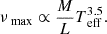
To quantify the best combination of models for the primary and secondary from the model grid generated in Sect. 3, we compare the modeled parameters for each timestep to the spectroscopic and seismic observables (Sect. 2). We used a reduced χred2-minimization approach whose general form is given by
 (2)
(2)
for a model with N parameters, where yn, obs represents the observed quantity and yn, mod the respective quantity from modeling, with σn being the observational error and n being the number of observables and m the number of fitted parameters. For every model combination, we determine the timestep of the lowest χred2, referred to as χmin2, and compare those minima with each other in our further analysis.
The dynamical choice of timesteps between consecutive models in MESA, as described in Paxton et al. (2011), causes the timesteps to be non-uniform. We interpolate the steps in the time domain for every relevant parameter for each given model track to compare two models at identical times before performing the χred2 calculation. This ensures that both components have the same age (Age1 = Age2). We rebinned the secondary’s evolutionary tracks to the primary’s timesteps. Models younger than 0.5 Gyr are removed to prevent false minima in the χred2 calculation when the star passes close to the observed values on the HRD during the pre-main-sequence phase. The frequency of maximum oscillation is calculated from the model’s position on the HRD using the scaling relations (Kjeldsen & Bedding 1995).
For the χred2 calculation, we allowed every combination of the models (representing the primary and secondary, respectively) that fulfilled the criteria that the mass of the primary was equal to or larger than the mass of the secondary (M2 ≤ M1) due to the solid constraint of the spectroscopic mass ratio q = M1/M2 = 1.015 ± 0.005.
4.2. Error estimation
As outlined in Sect. 1, error estimation is crucial in stellar age determination. Equation (2) considers the observables’ reported uncertainties (Sect. 2). The estimation of errors from the minimization in the χ2 statistics for the fitted parameter σi, y is given as (Bevington & Robinson 2003)
 (3)
(3)
with σn being the statistical error from the respective observable. If the smallest χred2 is above one, we assume the observational uncertainty as an error for our analysis because lower (formal) uncertainties do not have a physical meaning in this context. This approach, however, does not appropriately work for age estimation since there is no trivial mathematical description connecting the input parameters with the respective age of the system.
For the error determination in age from the calculated χred2, we evaluate all χred2 < 1, which, from a statistical viewpoint, have the same significance. From the scatter in age for these values with the same significance, we determine the edges of the area of confidence and give them as the upper and lower boundaries for the 1-σ uncertainty level. In case singular model points occur at a significantly higher or lower age with χred2 < 1, we test if those are consistent with stellar models for the observational mass/metallicity, and if not, remove them as outliers from the analysis.
Besides statistical errors, we are aware that the fitting procedure itself can introduce biases into the results of the modeling (e.g., Valle et al. 2014, 2015). Therefore, we applied a consistency check by recovering the secondary’s parameters from the primary’s HRD position and age using two model tracks with the same initial parameters, only differing in the mass by the mass ratio q. We were successfully able to recover the secondary’s HRD position within the margins of the 1-σ uncertainties of the observables.
5. Determination of the best-fitting models for different sets of parameters
Using the figure of merit defined in Sect. 4.1, in this section we test different parameter combinations for calculating χred2. In the following subsections we discuss the results of several cases where different sets of observables and constraints are used to find the best-fit model. The cases are summarized in Table 3. To show the improvements from strongly physically motivated parameter combinations, we also provide cases as a reference point that are less physically motivated but commonly used if fewer observational constraints are available.
Cases considered for modeling KIC 9163796 and the associated constraints.
5.1. Case A: Modeling of spectroscopic constraints
Using the χred2 figure of merit introduced in its general form in Eq. (2), we first define the ‘spectroscopic case’. The parameters used are the effective temperatures, Teff,1 and Teff,2, the surface gravities log g1 and log g2 of the primary and secondary component, respectively as well as the mass ratio q from spectroscopy. As we used the metallicity as an input parameter of the grid, we did not include it in the figure of merit, to avoid a circular argument. This parameter combination results in the formulation of the χred2 estimation for case A to be
 (4)
(4)
where each χred2 is calculated according to the term after the sum in Eq. (2).
To exploit the potential provided by the co-evolution of the two components of the binary system, we subsequently apply stronger constraints justified by their stellar binarity and evolutionary history. We generate four different cases for each formulation of the figure of merit. In the simplest case, A0, the residuals according to Eq. (4) are calculated for all the combinations of models that satisfy the aforementioned mass constraint, M2 ≤ M1, independent of the primary’s or secondary’s model metallicity. Given that both stars were born from the same cloud, we applied constraints on the metallicity. For simplicity, this work assumes the initial heavy element abundance equaling the current heavy element abundance. We tested if the assumption of Z = Zini causes deviations in our parameter determination but received a null result since the theoretical difference between the initial and current metallicity is at least one order of magnitude smaller than the uncertainty from the spectroscopic observations (Salaris 2006; Nissen & Gustafsson 2018). For the case A1, we required the metallicity of the components to be equal (binary condition, Z1 = Z2). In the case of A2, we enforce the same condition but additionally require the metallicity to be equal to the spectroscopic value (Z1, 2 = Zspec). For case A3, we allow metallicities to vary within their 1-σ uncertainty around the spectroscopic value (Z1, 2 = Zspec ± σZspec). For all three cases A1-A3, we also force the initial helium to be identical for the primary and secondary (Y1 = Y2).
We compared the χred2 distribution as a function of the age of the cases A0–A3 in Fig. 2. The age of the system for the different cases is taken from the mean of all χred2 values present below 1, with the errors estimated as described in Sect. 4.2. The least constrained case A0 provides an age of  Gyr, the three cases with increasing constraints, A1, A2, and A3 lead to ages of
  Gyr, 2.08
  Gyr and
  Gyr, respectively. Additionally, the minimum χred2 increases by about an order of magnitude toward χred2 = 1 for each case (A0 to A3).
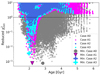 |
Fig. 2. Comparison of the best-fitting solutions for case A regarding the treatment of metallicity. The gray solutions have the metallicity varying freely in the modeled range (Case A0), the magenta solution only allows values where the metallicity of the primary equals the metallicity of the secondary (Case A1), while the royal blue solutions force both metallicities to be equal to the spectroscopic solution (Case A2). The cyan part only allows values in the range of 1σ around the spectroscopic value (Case A3). The magenta triangle, blue cross, and gray dot mark the respective minima of the corresponding datasets. The dashed horizontal line shows where χred2 = 1. |
Figure 3 shows the χred2 in the plane of the masses of the primary and secondary components for case A1 and the associated best-fitting solution. A clear trend following a diagonal line is visible, corresponding to the spectroscopic mass ratio q = 1.015. For case A0 and A1 we observe the best fitting solution at masses of M1 = 1.35 ± 0.06 M⊙ and M2 = 1.33 ± 0.06 M⊙. Only for case A2 do we observe slightly higher masses of M1 = 1.36 ± 0.06 M⊙ and M2 = 1.34 ± 0.06 M⊙.
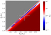 |
Fig. 3. Secondary mass and χred2-minima as a function of primary mass from the models with the condition of equal metallicity for the components Z1 = Z2 (Case A1). The color bar indicates the respective χred2-minima on a logarithmic scale. The residuals were calculated with enforcing M1 ≥ M2; the gray area represents the respective space where no χred2 is calculated due to this condition. The seismic solution, including its error bars from BKP18, is given in black, the absolute χred2-minimum is given in magenta triangle, and the green line represents the spectroscopic mass ratio of q = 1.015. |
5.2. Case B: Modeling including νmax constraint
To evaluate the surplus of additional asteroseismic constraints provided by the stellar oscillations, we now introduce the global seismic parameters νmax the figure of merit (case B). The corresponding value of the primary’s νmax of the stellar models is obtained with the scaling relations (Kjeldsen & Bedding 1995). Because νmax is strongly correlated with the surface gravity g via the scaling relations (Brown et al. 1991; Kjeldsen & Bedding 1995; Kallinger et al. 2014),
 (5)
(5)
we removed the latter as an observable. Therefore, the formulation of the figure of merit for case B is
 (6)
(6)
For case B, the minima of the χred2 for the model combination in the age-χred2 plane is given in Fig. 4. The cases B1, B2, and B3 lead to ages between 2.09 and 2.22 Gyr, with the exact values in Table 4. While the minima for case B1 (Z1 = Z2) is prominent, the minima for B2 (Z1, 2 = Zspec) and B3 (Z1, 2 = Zspec ± σ) are more spread out, suggesting that constraints beyond binarity could lead to an over-fitted solution. Regarding the mass, the best fitting model suggests a primary mass of M1 = 1.37 ± 0.06 M⊙, and secondary mass of M2 = 1.35 ± 0.06 M⊙, located at the upper end of the 1-σ errorbars from observation. All cases B1-B3 suggest a spectroscopic metallicity of Z1, 2 = 0.006 ± 0.002 and a helium abundance of Y1, 2 = 0.30 ± 0.03.
Cases considered for modeling KIC 9163796 and the associated stellar parameters determined from χred2-minimization.
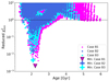 |
Fig. 4. Comparison of the best-fitting solutions regarding the treatment of metallicity for the case of including νmax in the figure of merit (Case B). The magenta solution only allows values where the metallicity of the primary equals the metallicity of the secondary (Case B1), while the royal blue solutions force both metallicities to be equal to the spectroscopic solution (Case B2). The cyan part only allows values in the range of 1σ around the spectroscopic value (Case B3). Symbols and colors are identical to Fig. 2. |
5.3. Case C: Modeling including Δν constraint
As a next step, we included Δν of the primary in the figure of merit. Therefore, the figure of merit for our case C reads as
 (7)
(7)
The addition of Δν in the figure of merit should bring the advantage of being independent of scaling relations but instead rely on observed frequencies. The large frequency separation is calculated using GYRE as outlined in Sect. 3. Again, the numbering of the cases C1 to C3 corresponds to the same constraints on mass, metallicity, and initial helium as described for the cases of the groups A and B and are listed in Table 3.
Using this new set of observables, the best-fit models have ages in the range of between 2.25 Gyr and 2.35 Gyr (Table 4), with the variation between the cases with the different initial metallicity constraints, C1 to C3, being less than 0.1 Gyr (Fig. 5). Regarding the mass, the best-fitting models point to a lower mass than in previous cases, down to M1 = 1.31 ± 0.06 M⊙ and M2 = 1.29 ± 0.06 M⊙, in case of cases C2 and C3, for the primary and secondary mass, respectively (Fig. 6).
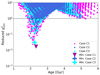 |
Fig. 5. Comparison of the best-fitting solutions regarding the treatment of metallicity, with the figure of merit used including the local Δν and νmax of the primary in the figure of merit (Case C). The magenta solution only allows values where the metallicity of the primary equals the metallicity of the secondary (Case C1), while the royal blue solutions force both metallicities to be equal to the spectroscopic solution (Case C2). The cyan part only allows values in the range of 1σ around the spectroscopic value (Case C3). Symbols and colors are identical to Fig. 2. |
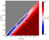 |
Fig. 6. Residuals of the χred2-minimization as a function of the primary mass M1 and secondary mass M2 with the condition of equal metallicity within the uncertainty range of the spectroscopic value of the components Z1, 2 = Zspec ± σZspec (Case C3), with the inclusion of Δν in the figure of merit. Colors and symbols are the same as in Fig. 3. We added the revised seismic masses obtained from the corrected Δν value as an orange cross. |
5.4. Case D: Modeling including magnitude difference
Up to this point, we have used more constraints regarding the primary than the secondary. One additional constraint we could use is the frequency of maximum oscillation νmax of the secondary. As described in Sect. 2, its νmax is reflected from the super-Nyquist regime and overlaps with the power excess of the primary and has been estimated using spectroscopic parameters, already included in the figure of merit. Therefore, we refrain from using νmax of the secondary as an additional observable. The frequency of maximum oscillations νmax is correlated with the total luminosity L of a star (Brown et al. 1991) by
 (8)
(8)
Because both components are at the same distance from us and affected by the same extinction, we can use the difference between the two absolute magnitudes as a proxy for the luminosity difference, and hence derive νmax of the secondary. The magnitude difference between the two components was inferred by BKP18 using the spectroscopic parameters (Table 1) and the total flux of the system in Johnson V. This led to an estimation of Δmv = 0.58 ± 0.08. The theoretical value is calculated as the difference of the default MESA output of magnitudes in Johnson V between the model of the primary and secondary at every timestep.
We therefore extended case C with the magnitude difference as an additional parameter. We define case D as
 (9)
(9)
Adding the magnitude difference as an observable results in a distinct distribution of χred2-minima over age (Fig. 7). For all cases, the χred2 values are close to 1. The ages of the best fitting model combinations for case D range from 2.44 Gyr to 2.58 Gyr, with uncertainties in the same order of magnitude as in case C (Table 4). The masses given by this model case resemble those of cases C2 and C3, with cases D1 being 0.01 M⊙ lower than the masses for cases D2 and D3 (M1 = 1.32 ± 0.06 M⊙ and M2 = 1.30 ± 0.06 M⊙, Fig. 8).
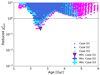 |
Fig. 7. Comparison of the best-fitting solutions regarding the treatment of metallicity for the case that includes the local Δν of the primary and the magnitude difference of the components in the figure of merit (Case D). The magenta solution only allows values where the metallicity of the primary equals the metallicity of the secondary (Case D1), while the royal blue solutions force both metallicities to be equal to the spectroscopic solution (Case D2). The cyan part only allows values in the range of 1σ around the spectroscopic value (Case D3). Symbols and colors are identical to Fig. 2. |
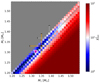 |
Fig. 8. Residuals of the χred2-minimization as a function of the primary mass M1 and secondary mass M2 with the condition of equal metallicity within the uncertainty range of the spectroscopic value of the components Z1, 2 = Zspec ± σZspec (Case D3); with the inclusion of Δν and the magnitude difference Δm in the figure of merit. Colors and symbols are the same as in Fig. 3. We added the revised seismic masses obtained from the corrected Δν value as an orange cross. |
As another aspect, we consider the variations in initial helium abundance and its effect on the best-fitting model in Fig. 9. For case D3 the models suggest helium abundances Y1, 2 = 0.29. This is also true if we do not force any binary condition regarding the helium abundances. Regarding the stellar metallicity, Fig. 10 depicts an example of the figure of merit as a function of metallicity and mass for the metallicity restricted to case D3. We observe a clear tendency to low metallicity, and the best fitting models all relax around Z1, 2 = 0.005.
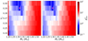 |
Fig. 9. Residuals of χred2-minimization in the mass-initial helium plane for both components (primary left, secondary right) for case D3. The best-fitting solution for each is marked as a magenta triangle. |
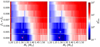 |
Fig. 10. Residuals of the χred2-minimization in the mass-metallicity plane for both components (primary left, secondary right) for identical metallicities for both components (Case D1). For this case, the magenta triangle marks the best-fitting solution. For the analogous case, with both model metallicities forced to be in the 1-σ-uncertainty of the spectroscopic value (Case D3), the best fitting solution is given as a blue cross. The dashed lines show the 1σ-errorbar around the spectroscopic metallicity. |
6. Discussion
Here, we compare the results for the stellar age and fundamental parameters of KIC 9163796 derived in the previous section and place them in the context of existing modeling/observational studies in the literature. We focus on cases C and D because these are the most physically motivated ones (Sect. 5).
6.1. Stellar age
A comparison of the age determination results for models using the different observables and constraints (cases A to D, including the subcases) is shown in Fig. 11. The least constrained case A0 provides an age estimation of 2.68 Gyr with an absolute age range within the error bars of σt (A0) = 4.4 Gyr (∼100%). The results for this case are similar to a single star or components of an unconstrained binary and serve as a reference point if no additional constraints are available. Applying the binary condition of Z1 = Z2 in cases A1, A2, and A3 reduces the uncertainty in the age of the models and raises the respective χred2-minima toward one, demonstrating that constraints from binarity help break degeneracies in parameter space. For cases B, where νmax is applied in addition to the spectroscopic constraints, consistent ages at around 2.0 Gyr arise from the modeling. All three subcases of case B exhibit error bars of similar size, indicating that the impact of νmax in the figure of merit overwrites the effect of the constraints from binarity. Additionally, we note that the difference in uncertainty between cases A and B could be due to competing minima from pure spectroscopic (cases A) and spectroscopic and asteroseismic (cases B) parameters.
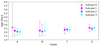 |
Fig. 11. Age estimations for the different cases of the figure of merit, including their uncertainties. The cases are calculated as described in Sect. 4, with the cases color coded as follows: magenta: Z1 = Z2; royal blue: Z1, 2 = Zspec; cyan: Z1, 2 = Zspec ± σZspec. |
If we move to cases where we use all seismic with all binary constraints the centroids for the ages are slightly higher compared to the previous cases (between 2.25 Gyr for case C3 to 2.35 Gyr for case C2), the respective ranges in uncertainties are considerably smaller, with the value for C2, being σt (C2) = 0.48 Gyr (∼10%). Furthermore, similarly to case B, we note that more constraints lead to a χred2 value closer to 1, hence more realistic physical models.
We see a very similar picture for cases D, where the magnitude difference is also included in addition to the spectroscopic and seismic constraints. Case D1 provides the highest age estimation of all binary constrained models with an age of 2.58 Gyr, with an errorbar range of σt (D1) = 0.81 Gyr. This result can likely be attributed to the χred2 distribution being flat at the minimum point of case D1, with several models with almost identical χred2 values but ages varying from 2.2 Gyr and 2.6 Gyr. Case D2 behaves almost identically to case C2 regarding the value and the error bars, suggesting that the metallicity restriction overrides any effects introduced by the magnitude difference. Both subcases (C2 and D2) provide similarly sized uncertainties (σt (C2) = 0.48 Gyr and σt (D2) = 0.45 Gyr), hence being the only cases with a relative age uncertainty below 10%. Conclusively, case D3 provides an age of 2.52 Gyr, with an uncertainty of σt (D3) = 0.67 Gyr, hence about 13% but in the same order of magnitude as for Cases C2 and D2. Cases D2 and D3 are also the most physically motivated ones, as they include all relevant parameters from spectroscopy, asteroseismology, and photometry in addition to reasonable binary constraints regarding the chemical abundances. These cases result in age uncertainties of 9% and 13%, respectively.
The best fitting ages determined from all cases, including seismic constraints (B, C, D), lead to consistent age determinations with scatter of about 12%. As visible from Fig. 11, the cases including Δν as a constraint (case C and D) provide ages that are ∼0.4 Gyr higher compared to respective subcases of cases A and B. Conclusively, all ages determined agree within uncertainties.
6.2. Stellar mass
The masses determined from the modeling for the different observables and constraints are depicted in Fig. 12. It can be seen that the masses for cases C and D (including the constraint of Δν) are on average around 5% lower than those for cases A and B (no Δν constraint). To consistently compare the masses from modeling with the observed seismic masses, we need to redetermine the masses from the scaling relations, taking the correction factor fΔν introduced in Sect. 5.2 into account. Using Eq. (14) from Li et al. (2023) and a fΔν = 0.974, derived from the centroids of the observational parameters of the primary and Eq. (16) from Li et al. (2023), leads to a revised primary mass of M1 = 1.35 ± 0.06 M⊙ and, using the mass ratio from spectroscopy, a secondary mass of M2 = 1.33 ± 0.06 M⊙.
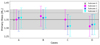 |
Fig. 12. Mass estimations for the primary for different cases of the figure of merit, including their uncertainties. The color coding is the same as in Fig. 11. The black solid line indicates the revised mass estimation from observations, with the gray area indicating the respective 1-σ error. The gray dashed line indicates the mass as given in BKP18. |
All values from our modeling fall well within the 1σ uncertainties of the scaling-based mass of the components (Fig.12) and also agree with one another within uncertainties. This is an important indication of our model correctly reproducing the two stellar components of KIC 9163796. When including the local Δν in the figure of merit in case C, we observe slightly lower masses for the more constrained cases C2 and C3, with primary masses for those cases being 1.31 M⊙. For case D, where we include the magnitude difference into the figure of merit, we receive similarly low masses as in case C, with the primary mass between 1.31 M⊙ to 1.32 M⊙ and the secondary mass between 1.29 M⊙ to 1.30 M⊙. This behavior indicates that mass estimations, including νmax and Δν, tend to provide slightly lower mass models than results solely from spectroscopy. Eventually, this is consistent with the higher ages obtained for cases C and D discussed in the previous subsection (Fig. 11). The mass consistency among cases C and D aligns with those cases being the most physically motivated ones.
As shown in Fig. 3, 6 and 8 the mass ratio is clearly reproduced when the residuals are plotted in the M1–M2 plane. Experiments have shown that this is also the case if q is not included in the figure of merit. For all cases, invariant of constraints or different figures of merit, the mass ratio q = 1.015 is always conserved, hence pointing to the mass ratio as a unique benefit and reliable constraint arising from the SB2 nature of the system.
6.3. Convective mixing length
The exact value for αMLT varies between the cases without any obvious correlations (Table 2). This behavior might be caused by the model correcting itself for possible systematic problems in the surface temperature measurements. However, the αMLT for the primary is lower or equal to the αMLT of the secondary for most of the cases, except case D. This pattern of αMLT, 1 ≤ αMLT, 2 indicates that the αMLT might not be constant over the evolution of a star, but rather it could decrease as the star rises on the SGB or RGB when the extension on the super-adiabatic region strongly increases. This result appears to provide some support to previous mixing-length calibration studies, such as Joyce & Tayar (2023), Trampedach et al. (2014), as well as it shows that relying on a single solar-calibrated αMLT value in stellar modeling might not be fully advisable, especially for stars whose mass, evolutionary stage and/or chemical composition are significantly different than those of Sun-like stars. For instance, Tayar et al. (2017) suggested that the super-adiabatic convection efficiency should decrease with decreasing metal abundance, but on the same topic Salaris et al. (2018) – by using a different set of model predictions – have obtained a quite different conclusion, and have shown that the exact heavy element distribution (solar scaled versus α−enhanced one) plays a role in the comparison between observations and stellar models. However, as concluded in Joyce & Tayar (2023) and from results of synthetic studies (e.g., Valle et al. 2019), any direct dependence of mixing length on metallicity should be dealt with caution. Needless to say, to shed light on this important topic, it is important to increase the sample of (binary) stars with accurately determined physical properties.
As we have limited the range for αMLT as described in Appendix A using the spectroscopic case A, we retested if, for the Cases B to D, better fitting models occur outside the limited range. This test confirmed our choice of limiting αMLT, as no best-fitting models outside the range were found.
6.4. Initial He and metallicity
Regarding the initial helium abundance, there is a distinct trend. Without exception, all cases show an initial helium abundance greater than the generally accepted primordial helium abundance of 0.24 (Charbonnel et al. 2017). The modeled helium abundances range from 0.27 to 0.30, with a formal uncertainty of ±0.03. Due to the comparatively young age of the system of around 2 Gyr, born around 11 Gyr after the Big Bang, this enriched initial helium value is quite plausible and also consistent with the modeling of similar - although single – stars (Verma et al. 2019). Furthermore, enforcing stronger metallicity constraints, as in cases 2 and 3, respectively, leads to higher initial helium abundances than those with less stringent or no constraints (subcases 0 and 1). As some of the recovered initial helium values are located at the edge of the explored range, we explored the modeling grid with a higher upper boundary of Yini = 0.33. The majority of results results were unchanged with this expanded range. However, for two subcases (C2 and D2) we recovered higher abundances, again at the edge of the explored range (Yini = 0.32 and Yini = 0.33, respectively). This edge effect could be related to the effect recovered from synthetic modeling by Valle et al. (2024), who demonstrate that, independent of the fitting method, helium abundances in grid modeling are biased toward the edges of the explored ranges.
Comparing the results for the metallicity of the best-fitting models, it occurs that subcases 1, with no numerical restriction for the initial heavy element abundance, generally exhibit a Z value at the lower boundary of the model grid range (Z1, 2 = 0.004 ± 0.002). This is significantly lower than the spectroscopic value for Z, even when accounting for the observational errors (Fig. 10). Also, case A0, with no binarity constraints, exhibits an initial heavy metal abundance of Z1, 2 = 0.004 ± 0.002. Following directly from the constraints in cases 2 and 3, forcing both components to the spectroscopic and spectroscopic metallicity, including the 1-σ observational error bars, respectively, lead to higher metallicities, as shown in Table 4. Apart from this trend, we observe no clear correlations in the results for metallicity. However, it is a crucial parameter for constraining the model parameter space, particularly for the age determination, as we have demonstrated in Sect. 6.1.
6.5. Figures of merit and model uncertainty
Eventually, it should be noted that – following the description in Sect. 4.2 – all uncertainties for stellar parameters, except the age, are dominated by the observational uncertainties of the input parameters. Therefore, an improvement in the uncertainty of those parameters would directly lead to an improvement in the model uncertainties. Across all cases, subcase 2 systematically has smaller uncertainties because it is chosen for a single metallicity bin, while subcases 3 take a wider bin and therefore allows for more combinations, which increases the uncertainty. As cases D demonstrate the most consistent age estimations, and exhibit a χred2 closest to unity, and include all relevant parameters from spectroscopy, asteroseismology, and photometry in addition to reasonable binary constraints, we consider them to be the most physically motivated ones.
7. Conclusion
In this work, we have performed comprehensive modeling of the red giant-subgiant asteroseismic SB2 binary system KIC 9163796. We built a multidimensional grid in parameter space to accurately model the primary and secondary using the MESA stellar evolution code and GYRE oscillations code. By using constraints from spectroscopy, asteroseismology, and binarity and different formulations of a χred2 figure-of-merit, we determined the precise ages and stellar parameters (M, Z, Y, αMLT) for the binary system. These results are summarized in Table 4. From the results of the most physically motivated cases (Case D2 and D3, see Sect. 6.1), we adopt 2.44  Gyr (Case D2) as the age of the system.
All cases with binarity constraints tested in this work converge to ages within less than 20 % of each other, with a maximum of 2.58 Gyr (Case D1) and a minimum of 2.09 Gyr (Case B2 and B3), while the cases including all seismic constraints (C, D) lead to consistent age determinations as well (scatter of less than 13%). This demonstrates the robustness of age determination using the combined approach with data from spectroscopy, asteroseismology, and binarity. Additionally, we showed that, in particular, constraints from binarity lead to a significant improvement in age uncertainties, with the best case bringing them down to 9%, which represents an order of magnitude improvement compared to a modeling approach, without asteroseismic and binarity constraints (50–100%; see Table 4). Furthermore, across all modeling cases, the minimum χred2 values get closer to one when applying constraints from binarity, thus pointing to less overfitting and more realistic models. In addition, our analysis also demonstrates that adequately calibrated parameters from asteroseismology, in particular Δν, can lead to more precise age estimations compared to using only observables from spectroscopy (Fig. 11). We conclude that constraints from binarity and asteroseismology can break degeneracies and certain limitations arising from 1D modeling (e.g., see conclusions of Joyce & Tayar 2023) and improve the precision of age determination significantly.
With this detailed study, we demonstrate that well-modeled systems such as KIC 9163796, which are observationally well constrained from photometry, spectroscopy, and asteroseismology, have the diagnostic potential for testing the internal physics that is otherwise challenging to obtain from single star models. We showed this by constraining the initial helium abundance Y and the mixing-length parameter αMLT, which are usually inaccessible to observations. The higher-than-primordial initial helium abundance and the lower-than-solar αMLT shown in our modeling are compatible with the system’s age and evolutionary stage and are in agreement with previous studies. However, as discussed in Sect. 6.4, some of the recovered initial helium values could be affected by a general bias toward the grid edges (Valle et al. 2024).
This in-depth modeling demonstrates that KIC 9163796 is a benchmark system for constraining stellar age. As stated in Miglio et al. (2014), many constrained systems such as the prototype KIC 9163796 should exist; however, only a few have been found, and none has been modeled in such depth. Further analysis is necessary to find more oscillating binary systems similar to KIC 9163796 with similar constraints from seismology and binarity.
Possible further constraints, particularly for age determination, could arise from the study of eclipsing binary systems (Gaulme et al. 2022; Valle et al. 2023; Rowan et al. 2024) or stellar clusters (Brogaard et al. 2023; Reyes et al. 2024) containing solar-like oscillators. Beck et al. (2024) has reported over 900 new oscillating binary systems through cross-correlation of Gaia DR3 data with sample catalogs of solar-like oscillators. The authors suggest that astrometric binary systems for which an SB2 signature has been found could significantly expand the sample size of benchmark systems similar to KIC 9163796 in number, evolutionary state, and parameter space. Also, using individual frequencies of the modes in future modeling can help further improve the estimation of stellar ages and other parameters (Li et al. 2022, 2024).
Future asteroseismic space missions, particularly the ESA PLATO Mission (Rauer et al. 2014, 2024), will be able to provide high signal-to-noise asteroseismic data of thousands of unstudied main-sequence and red giant oscillators. In particular, the Science Validation and Calibration PLATO Target Input Catalogue (scvPIC) contains several thousand potential benchmark binary systems with known inclinations, which potentially host main-sequence or giant solar-like oscillators. Using these future datasets in combination with existing ones, such as the Apache Point Observatory Galactic Evolution Experiment (APOGEE; Majewski et al. 2017) and Gaia (Gaia Collaboration 2016), and extending them through ground-based follow-up programs will enable the use of constraints from asteroseismology, spectroscopy, and binarity to advance knowledge about the Milky Way’s history, dynamics, and chemical composition in the context of Galactic archaeology.
KIC 9163796 = TIC 271664383, Gaia DR3 2079986695058294272, and 2MASS J19412099+4530173.
Available at https://github.com/rjfarmer/multimesa
Acknowledgments
We thank the referee, Pier Giorgio Prada Moroni, for constructive comments that improved the paper. The authors thank the people behind the ESA Gaia, NASA Kepler, and NASA TESS missions and HERMES spectrograph. The authors thank the team of UniIT, especially Dr. Ursula Winkler and David Bodruzic is thanked for excellent support and maintanance of the High Performance Computing cluster of the University of Graz (Graz Scientific Cluster 1 – GSC 1), used for computations of this work. Further, thanks go to Roland Maderbacher and Klaus Huber for their support in high-performance computing. We also thank Anna Queiroz and Carlos Allende for the discussions that helped improve the target parameters. The project that gave rise to these results received the support of a fellowship from “la Caixa” Foundation (ID 100010434). The fellowship code is LCF/BQ/DI23/11990068. DHG acknowledges support of the Dr. Heinrich-Jörg Foundation at the Graz University. DHG and NM acknowledge travel support through the “Förderungsstipendium” provided by the Faculty of Natural Sciences of the Graz University. PGB acknowledges support by the Spanish Ministry of Science and Innovation with the Ramón y Cajal fellowship number RYC-2021-033137-I and the number MRR4032204. PGB, DHG, DGR, and RAG acknowledge support from the Spanish Ministry of Science and Innovation with the grant no. PID2023-146453NB-100 (PLAtoSOnG). DHG, SM, DGR, and RAG acknowledge support from the Spanish Ministry of Science and Innovation with the grant no. PID2023-149439NB-C41 (PLATO). SM acknowledges support by the Spanish Ministry of Science and Innovation with the grant no. PID2019-107061GB-C66 and through AEI under the Severo Ochoa Centres of Excellence Programme 2020–2023 (CEX2019-000920-S). SM and DGR acknowledges support from the Spanish Ministry of Science and Innovation with the grant no. PID2019-107187GB-I00. RAG acknowledges support from the PLATO Centre National D’Études Spatiales grant. DGR acknowledges support from the Juan de la Cierva program under contract JDC2022-049054-I. LS acknowledges the Graz University of Technology travel grant. SC has been funded by the European Union – “NextGenerationEU” RRF M4C2 1.1 n: 2022HY2NSX. “CHRONOS: adjusting the clock(s) to unveil the CHRONO-chemo-dynamical Structure of the Galaxy” (PI: S. Cassisi), and INAF 2023 Theory grant “Lasting” (PI: S. Cassisi). We gratefully acknowledge support from the Australian Research Council through Laureate Fellowship FL220100117, which includes a PhD scholarship for LSS. This work has made use of data from the European Space Agency (ESA) mission Gaia (https://www.cosmos.esa.int/gaia), processed by the Gaia Data Processing and Analysis Consortium (DPAC, https://www.cosmos.esa.int/web/gaia/dpac/consortium). Funding for the DPAC has been provided by national institutions, particularly the institutions participating in the Gaia Multilateral Agreement. This paper includes data collected with the Kepler & TESS missions obtained from the MAST data archive at the Space Telescope Science Institute (STScI). Funding for these missions is provided by the NASA Science Mission Directorate and the NASA Explorer Program. STScI is operated by the Association of Universities for Research in Astronomy, Inc., under NASA contract NAS 5–26555. This paper is partly based on observations obtained with the HERMES spectrograph, which is supported by the Research Foundation – Flanders (FWO), Belgium, the Research Council of KU Leuven, Belgium, the Fonds National de la Recherche Scientifique (F.R.S.-FNRS), Belgium, the Royal Observatory of Belgium, the Observatoire de Genève, Switzerland and the Thüringer Landessternwarte Tautenburg, Germany. Software: Python (Van Rossum & Drake 2009), numpy (Oliphant 2006; Harris et al. 2020), matplotlib (Hunter 2007), scipy (Virtanen et al. 2020), pandas (pandas development team 2020; McKinney et al. 2010), Astroquery (Ginsburg et al. 2019). This research made use of Astropy (Astropy Collaboration 2013); astropy:2018, a community-developed core Python package for Astronomy. This work has utilized the stellar evolutionary code package, Modules for Experiments in Stellar Astrophysics (MESA Paxton et al. 2011, 2013, 2015, 2018, 2019; Jermyn et al. 2023). The MESA EOS is a blend of the OPAL (Rogers & Nayfonov 2002), SCVH (Saumon et al. 1995), FreeEOS (Irwin 2004), HELM (Timmes & Swesty 2000), PC (Potekhin & Chabrier 2010), and Skye (Jermyn et al. 2021) EOSes. Radiative opacities are primarily from OPAL (Iglesias & Rogers 1993, 1996), with low-temperature data from Ferguson et al. (2005) and the high-temperature, Compton-scattering dominated regime by Poutanen (2017). Electron conduction opacities are from Cassisi et al. (2007) and Blouin et al. (2020). Nuclear reaction rates are from JINA REACLIB (Cyburt et al. 2010), NACRE (Angulo et al. 1999) and additional tabulated weak reaction rates Fuller et al. (1985), Oda et al. (1994), Langanke & Martinez-Pinedo (2000). Screening is included via the prescription of Chugunov et al. (2007). Thermal neutrino loss rates are from Itoh et al. (1996). This paper utilized the GYRE stellar oscillations code developed by Townsend & Teitler (2013).
References
- Andrae, R., Fouesneau, M., Sordo, R., et al. 2023, A&A, 674, A27 [CrossRef] [EDP Sciences] [Google Scholar]
- Angulo, C., Arnould, M., Rayet, M., et al. 1999, Nucl. Phys. A, 656, 3 [Google Scholar]
- Astropy Collaboration (Robitaille, T. P., et al.) 2013, A&A, 558, A33 [NASA ADS] [CrossRef] [EDP Sciences] [Google Scholar]
- Astropy Collaboration (Price-Whelan, A. M., et al.) 2018, AJ, 156, 123 [Google Scholar]
- Badenes, C., Mazzola, C., Thompson, T. A., et al. 2018, ApJ, 854, 147 [NASA ADS] [CrossRef] [Google Scholar]
- Bailer-Jones, C. A. L., Rybizki, J., Fouesneau, M., Demleitner, M., & Andrae, R. 2021, AJ, 161, 147 [Google Scholar]
- Beck, P. G., Hambleton, K., Vos, J., et al. 2014, A&A, 564, A36 [NASA ADS] [CrossRef] [EDP Sciences] [Google Scholar]
- Beck, P. G., do Nascimento, J. D., Duarte, T., et al. 2017, A&A, 602, A63 [NASA ADS] [CrossRef] [EDP Sciences] [Google Scholar]
- Beck, P. G., Kallinger, T., Pavlovski, K., et al. 2018, A&A, 612, A22 [NASA ADS] [CrossRef] [EDP Sciences] [Google Scholar]
- Beck, P. G., Mathur, S., Hambleton, K., et al. 2022, A&A, 667, A31 [NASA ADS] [CrossRef] [EDP Sciences] [Google Scholar]
- Beck, P. G., Grossmann, D. H., Steinwender, L., et al. 2024, A&A, 682, A7 [NASA ADS] [CrossRef] [EDP Sciences] [Google Scholar]
- Bevington, P., & Robinson, D. 2003, Data Reduction and Error Analysis for the Physical Sciences (McGraw-Hill Education) [Google Scholar]
- Blouin, S., Shaffer, N. R., Saumon, D., & Starrett, C. E. 2020, ApJ, 899, 46 [NASA ADS] [CrossRef] [Google Scholar]
- Borucki, W. J., Koch, D., Basri, G., et al. 2010, Science, 327, 977 [Google Scholar]
- Brogaard, K., Arentoft, T., Miglio, A., et al. 2023, A&A, 679, A23 [NASA ADS] [CrossRef] [EDP Sciences] [Google Scholar]
- Brown, T. M., Gilliland, R. L., Noyes, R. W., & Ramsey, L. W. 1991, ApJ, 368, 599 [Google Scholar]
- Campante, T. L., Li, T., Ong, J. M. J., et al. 2023, AJ, 165, 214 [NASA ADS] [CrossRef] [Google Scholar]
- Casagrande, L., Silva Aguirre, V., Schlesinger, K. J., et al. 2016, MNRAS, 455, 987 [Google Scholar]
- Cassisi, S., & Salaris, M. 2011, ApJ, 728, L43 [NASA ADS] [CrossRef] [Google Scholar]
- Cassisi, S., Potekhin, A. Y., Pietrinferni, A., Catelan, M., & Salaris, M. 2007, ApJ, 661, 1094 [NASA ADS] [CrossRef] [Google Scholar]
- Charbonnel, C., Decressin, T., Lagarde, N., et al. 2017, A&A, 605, A102 [NASA ADS] [CrossRef] [EDP Sciences] [Google Scholar]
- Chugunov, A. I., Dewitt, H. E., & Yakovlev, D. G. 2007, Phys. Rev. D, 76, 025028 [NASA ADS] [CrossRef] [Google Scholar]
- Constantino, T., Campbell, S. W., Christensen-Dalsgaard, J., Lattanzio, J. C., & Stello, D. 2015, MNRAS, 452, 123 [Google Scholar]
- Creevey, O. L., Cassisi, S., Thévenin, F., Salaris, M., & Pietrinferni, A. 2024, A&A, 689, A243 [NASA ADS] [CrossRef] [EDP Sciences] [Google Scholar]
- Cyburt, R. H., Amthor, A. M., Ferguson, R., et al. 2010, ApJS, 189, 240 [NASA ADS] [CrossRef] [Google Scholar]
- del Burgo, C., & Allende Prieto, C. 2018, MNRAS, 479, 1953 [Google Scholar]
- Ferguson, J. W., Alexander, D. R., Allard, F., et al. 2005, ApJ, 623, 585 [Google Scholar]
- Freeman, K., & Bland-Hawthorn, J. 2002, ARA&A, 40, 487 [Google Scholar]
- Fuller, G. M., Fowler, W. A., & Newman, M. J. 1985, ApJ, 293, 1 [NASA ADS] [CrossRef] [Google Scholar]
- Gaia Collaboration (Prusti, T., et al.) 2016, A&A, 595, A1 [NASA ADS] [CrossRef] [EDP Sciences] [Google Scholar]
- Gaia Collaboration (Vallenari, A., et al.) 2023a, A&A, 674, A1 [NASA ADS] [CrossRef] [EDP Sciences] [Google Scholar]
- Gaia Collaboration (Arenou, F., et al.) 2023b, A&A, 674, A34 [CrossRef] [EDP Sciences] [Google Scholar]
- García, R. A., Hekker, S., Stello, D., et al. 2011, MNRAS, 414, L6 [NASA ADS] [CrossRef] [Google Scholar]
- García, R. A., Ceillier, T., Salabert, D., et al. 2014a, A&A, 572, A34 [NASA ADS] [CrossRef] [EDP Sciences] [Google Scholar]
- García, R. A., Mathur, S., Pires, S., et al. 2014b, A&A, 568, A10 [Google Scholar]
- Gaulme, P., Borkovits, T., Appourchaux, T., et al. 2022, A&A, 668, A173 [NASA ADS] [CrossRef] [EDP Sciences] [Google Scholar]
- Ginsburg, A., Sipőcz, B. M., Brasseur, C. E., et al. 2019, AJ, 157, 98 [Google Scholar]
- Godoy-Rivera, D., Tayar, J., Pinsonneault, M. H., et al. 2021, ApJ, 915, 19 [NASA ADS] [CrossRef] [Google Scholar]
- Godoy-Rivera, D., Mathur, S., García, R. A., et al. 2025, A&A, in press https://doi.org/10.1051/0004-6361/202348735 [NASA ADS] [CrossRef] [EDP Sciences] [Google Scholar]
- Grevesse, N., & Sauval, A. J. 1998, Space Sci. Rev., 85, 161 [Google Scholar]
- Gustafsson, B., Edvardsson, B., Eriksson, K., et al. 2008, A&A, 486, 951 [NASA ADS] [CrossRef] [EDP Sciences] [Google Scholar]
- Harris, C. R., Millman, K. J., van der Walt, S. J., et al. 2020, Nature, 585, 357 [NASA ADS] [CrossRef] [Google Scholar]
- Heiter, U., Lind, K., Asplund, M., et al. 2015, Phys. Scr., 90, 054010 [Google Scholar]
- Howell, M., Campbell, S. W., Stello, D., & De Silva, G. M. 2024, MNRAS, 527, 7974 [Google Scholar]
- Hunter, J. D. 2007, Comput. Sci. Eng., 9, 90 [NASA ADS] [CrossRef] [Google Scholar]
- Iglesias, C. A., & Rogers, F. J. 1993, ApJ, 412, 752 [Google Scholar]
- Iglesias, C. A., & Rogers, F. J. 1996, ApJ, 464, 943 [NASA ADS] [CrossRef] [Google Scholar]
- Ilijic, S., Hensberge, H., Pavlovski, K., & Freyhammer, L. M. 2004, in Spectroscopically and Spatially Resolving the Components of the Close Binary Stars, eds. R. W. Hilditch, H. Hensberge, & K. Pavlovski, ASP Conf. Ser., 318, 111 [Google Scholar]
- Irwin, A. W. 2004, The FreeEOS Code for Calculating the Equation of State for Stellar Interiors [Google Scholar]
- Itoh, N., Hayashi, H., Nishikawa, A., & Kohyama, Y. 1996, ApJS, 102, 411 [NASA ADS] [CrossRef] [Google Scholar]
- Jermyn, A. S., Schwab, J., Bauer, E., Timmes, F. X., & Potekhin, A. Y. 2021, ApJ, 913, 72 [NASA ADS] [CrossRef] [Google Scholar]
- Jermyn, A. S., Bauer, E. B., Schwab, J., et al. 2023, ApJS, 265, 15 [NASA ADS] [CrossRef] [Google Scholar]
- Johnston, C., Tkachenko, A., Aerts, C., et al. 2019a, MNRAS, 482, 1231 [Google Scholar]
- Johnston, C., Pavlovski, K., & Tkachenko, A. 2019b, A&A, 628, A25 [NASA ADS] [CrossRef] [EDP Sciences] [Google Scholar]
- Joyce, M., & Tayar, J. 2023, Galaxies, 11, 75 [NASA ADS] [CrossRef] [Google Scholar]
- Kallinger, T., De Ridder, J., Hekker, S., et al. 2014, A&A, 570, A41 [NASA ADS] [CrossRef] [EDP Sciences] [Google Scholar]
- Kjeldsen, H., & Bedding, T. R. 1995, A&A, 293, 87 [NASA ADS] [Google Scholar]
- Kumar, P., Ao, C. O., & Quataert, E. J. 1995, ApJ, 449, 294 [Google Scholar]
- Langanke, K., & Martinez-Pinedo, G. 2000, Nucl. Phys. A, 673, 481 [NASA ADS] [CrossRef] [Google Scholar]
- Lebreton, Y., & Goupil, M. J. 2014, A&A, 569, A21 [NASA ADS] [CrossRef] [EDP Sciences] [Google Scholar]
- Li, T., Li, Y., Bi, S., et al. 2022, ApJ, 927, 167 [NASA ADS] [CrossRef] [Google Scholar]
- Li, Y., Bedding, T. R., Stello, D., et al. 2023, MNRAS, 523, 916 [NASA ADS] [CrossRef] [Google Scholar]
- Li, T., Bi, S., Davies, G. R., et al. 2024, MNRAS, 530, 2810 [CrossRef] [Google Scholar]
- Majewski, S. R., Schiavon, R. P., Frinchaboy, P. M., et al. 2017, AJ, 154, 94 [NASA ADS] [CrossRef] [Google Scholar]
- Masseron, T., Merle, T., & Hawkins, K. 2016, Astrophysics Source Code Library [record ascl:1605.004] [Google Scholar]
- Mathur, S., García, R. A., Breton, S., et al. 2022, A&A, 657, A31 [NASA ADS] [CrossRef] [EDP Sciences] [Google Scholar]
- McKinney, W. 2010, in Proceedings of the 9th Python in Science Conference, eds. S. van der Walt, & J. Millman, 56 [Google Scholar]
- Miglio, A., Chaplin, W. J., Farmer, R., et al. 2014, ApJ, 784, L3 [CrossRef] [Google Scholar]
- Moe, M., & Di Stefano, R. 2017, ApJS, 230, 15 [Google Scholar]
- Moser, S., Valle, G., Dell’Omodarme, M., Degl’Innocenti, S., & Prada Moroni, P. G. 2023, A&A, 671, A78 [NASA ADS] [CrossRef] [EDP Sciences] [Google Scholar]
- Murphy, S. J., Li, T., Sekaran, S., et al. 2021, MNRAS, 505, 2336 [NASA ADS] [CrossRef] [Google Scholar]
- Nissen, P. E., & Gustafsson, B. 2018, A&ARv, 26, 6 [Google Scholar]
- Oda, T., Hino, M., Muto, K., Takahara, M., & Sato, K. 1994, Atomic Data Nucl. Data Tables, 56, 231 [NASA ADS] [CrossRef] [Google Scholar]
- Offner, S. S. R., Moe, M., Kratter, K. M., et al. 2023, in Protostars and Planets VII, eds. S. Inutsuka, Y. Aikawa, T. Muto, K. Tomida, M. Tamura, et al., ASP Conf.Ser., 534, 275 [NASA ADS] [Google Scholar]
- Oliphant, T. 2006, NumPy: A guide to NumPy (USA: Trelgol Publishing) [Google Scholar]
- pandas development team 2020, https://doi.org/10.5281/zenodo.3509134 [Google Scholar]
- Paxton, B., Bildsten, L., Dotter, A., et al. 2011, ApJS, 192, 3 [Google Scholar]
- Paxton, B., Cantiello, M., Arras, P., et al. 2013, ApJS, 208, 4 [Google Scholar]
- Paxton, B., Marchant, P., Schwab, J., et al. 2015, ApJS, 220, 15 [Google Scholar]
- Paxton, B., Schwab, J., Bauer, E. B., et al. 2018, ApJS, 234, 34 [NASA ADS] [CrossRef] [Google Scholar]
- Paxton, B., Smolec, R., Schwab, J., et al. 2019, ApJS, 243, 10 [Google Scholar]
- Peimbert, M., Luridiana, V., & Peimbert, A. 2007, ApJ, 666, 636 [NASA ADS] [CrossRef] [Google Scholar]
- Pinsonneault, M. H., Elsworth, Y. P., Tayar, J., et al. 2018, ApJS, 239, 32 [Google Scholar]
- Pinsonneault, M. H., Zinn, J. C., Tayar, J., et al. 2025, ApJS, 276, 69 [NASA ADS] [CrossRef] [Google Scholar]
- Pires, S., Mathur, S., García, R. A., et al. 2015, A&A, 574, A18 [NASA ADS] [CrossRef] [EDP Sciences] [Google Scholar]
- Potekhin, A. Y., & Chabrier, G. 2010, Contrib. Plasma Phys., 50, 82 [NASA ADS] [CrossRef] [Google Scholar]
- Poutanen, J. 2017, ApJ, 835, 119 [NASA ADS] [CrossRef] [Google Scholar]
- Prša, A. 2018, Phoebe 2 - Modeling and Analysis of Eclipsing Binary Stars [Google Scholar]
- Raghavan, D., McAlister, H. A., Henry, T. J., et al. 2010, ApJS, 190, 1 [Google Scholar]
- Raskin, G., Van Winckel, H., Hensberge, H., et al. 2011, A&A, 526, A69 [CrossRef] [EDP Sciences] [Google Scholar]
- Rauer, H., Catala, C., Aerts, C., et al. 2014, Exp. Astron., 38, 249 [Google Scholar]
- Rauer, H., Aerts, C., Cabrera, J., et al. 2024, ArXiv e-prints [arXiv:2406.05447] [Google Scholar]
- Rawls, M. L., Gaulme, P., McKeever, J., et al. 2016, ApJ, 818, 108 [Google Scholar]
- Remus, F., Mathis, S., & Zahn, J. P. 2012, A&A, 544, A132 [NASA ADS] [CrossRef] [EDP Sciences] [Google Scholar]
- Reyes, C., Stello, D., Hon, M., et al. 2024, MNRAS, 532, 2860 [NASA ADS] [CrossRef] [Google Scholar]
- Ricker, G. R., Winn, J. N., Vanderspek, R., et al. 2014, in Space Telescopes and Instrumentation 2014: Optical, Infrared, and Millimeter Wave, eds. J. Oschmann, M. Jacobus, M. Clampin, G. G. Fazio, H. A. MacEwen, et al., SPIE Conf. Ser., 9143, 914320 [Google Scholar]
- Roberts, J. D., Pinsonneault, M. H., Johnson, J. A., et al. 2024, MNRAS, 530, 149 [Google Scholar]
- Rogers, F. J., & Nayfonov, A. 2002, ApJ, 576, 1064 [Google Scholar]
- Rowan, D. M., Stanek, K. Z., Kochanek, C. S., et al. 2024, ArXiv e-prints [arXiv:2409.02983] [Google Scholar]
- Salabert, D., García, R. A., Beck, P. G., et al. 2016, A&A, 596, A31 [NASA ADS] [CrossRef] [EDP Sciences] [Google Scholar]
- Salaris, M. 2006, From theory to observation (John Wiley& Sons, Ltd), 239 [Google Scholar]
- Salaris, M., Cassisi, S., Schiavon, R. P., & Pietrinferni, A. 2018, A&A, 612, A68 [NASA ADS] [CrossRef] [EDP Sciences] [Google Scholar]
- Saumon, D., Chabrier, G., & van Horn, H. M. 1995, ApJS, 99, 713 [NASA ADS] [CrossRef] [Google Scholar]
- Sekaran, S., Johnston, C., Tkachenko, A., et al. 2019, A&A, 624, A140 [EDP Sciences] [Google Scholar]
- Soderblom, D. R. 2010, ARA&A, 48, 581 [Google Scholar]
- Tayar, J., Somers, G., Pinsonneault, M. H., et al. 2017, ApJ, 840, 17 [NASA ADS] [CrossRef] [Google Scholar]
- Thompson, S. E., Everett, M., Mullally, F., et al. 2012, ApJ, 753, 86 [Google Scholar]
- Timmes, F. X., & Swesty, F. D. 2000, ApJS, 126, 501 [NASA ADS] [CrossRef] [Google Scholar]
- Townsend, R. H. D., & Teitler, S. A. 2013, MNRAS, 435, 3406 [Google Scholar]
- Trampedach, R., Stein, R. F., Christensen-Dalsgaard, J., Nordlund, Å., & Asplund, M. 2014, MNRAS, 445, 4366 [NASA ADS] [CrossRef] [Google Scholar]
- Ulla, A., Creevey, O. L., Álvarez, M. A., et al. 2022, Gaia DR3 documentation Chapter 11: Astrophysical parameters, Gaia DR3 documentation, European Space Agency; Gaia Data Processing and Analysis Consortium, 11 [Google Scholar]
- Valle, G., Dell’Omodarme, M., Prada Moroni, P. G., & Degl’Innocenti, S. 2013, A&A, 549, A50 [CrossRef] [EDP Sciences] [Google Scholar]
- Valle, G., Dell’Omodarme, M., Prada Moroni, P. G., & Degl’Innocenti, S. 2014, A&A, 561, A125 [NASA ADS] [CrossRef] [EDP Sciences] [Google Scholar]
- Valle, G., Dell’Omodarme, M., Prada Moroni, P. G., & Degl’Innocenti, S. 2015, A&A, 575, A12 [NASA ADS] [CrossRef] [EDP Sciences] [Google Scholar]
- Valle, G., Dell’Omodarme, M., Prada Moroni, P. G., & Degl’Innocenti, S. 2018, A&A, 615, A62 [NASA ADS] [CrossRef] [EDP Sciences] [Google Scholar]
- Valle, G., Dell’Omodarme, M., Prada Moroni, P. G., & Degl’Innocenti, S. 2019, A&A, 623, A59 [NASA ADS] [CrossRef] [EDP Sciences] [Google Scholar]
- Valle, G., Dell’Omodarme, M., Prada Moroni, P. G., & Degl’Innocenti, S. 2023, A&A, 673, A133 [NASA ADS] [CrossRef] [EDP Sciences] [Google Scholar]
- Valle, G., Dell’Omodarme, M., Prada Moroni, P. G., & Degl’Innocenti, S. 2024, A&A, 687, A294 [NASA ADS] [CrossRef] [EDP Sciences] [Google Scholar]
- Van Rossum, G., & Drake, F. L. 2009, Python 3 Reference Manual (Scotts Valley, CA: CreateSpace) [Google Scholar]
- Verma, K., Raodeo, K., Basu, S., et al. 2019, MNRAS, 483, 4678 [Google Scholar]
- Verma, K., Rørsted, J. L., Serenelli, A. M., et al. 2022, MNRAS, 515, 1492 [NASA ADS] [CrossRef] [Google Scholar]
- Virtanen, P., Gommers, R., Oliphant, T. E., et al. 2020, Nature Methods, 17, 261 [CrossRef] [Google Scholar]
- Wang, T., Chen, B.-Q., Lian, J.-H., Xiang, M.-S., & Liu, X.-W. 2024, MNRAS, 533, L31 [NASA ADS] [CrossRef] [Google Scholar]
- Warfield, J. T., Zinn, J. C., Schonhut-Stasik, J., et al. 2024, AJ, 167, 208 [NASA ADS] [CrossRef] [Google Scholar]
- Welsh, W. F., Orosz, J. A., Aerts, C., et al. 2011, ApJS, 197, 4 [Google Scholar]
- Zahn, J.-P. 1975, A&A, 41, 329 [Google Scholar]
Appendix A: Adjustment of αMLT
As recently summarized by Joyce & Tayar (2023), the application of one-dimensional mixing-length theory in 1D modeling and, in particular, the choice of αMLT is a complex topic and can have a significant impact on modeled fundamental parameters and degeneracies with other physical parameters and also the stellar age. For computational efficiency, we decided to narrow down the range of αMLT before proceeding with the investigation. We have decided to calibrate the mixing length by testing the impact of a changing αMLT on the best-fitting models of the previously introduced spectroscopic case.
For the adjustment of the αMLT we have used the figure of merit with parameter set from case A1 (Sect. 5.1) as a benchmark. Figure A.1 depicts the position of the ten model combinations with the lowest χred2 for each choice of αMLT on a HRD-like plane. We observed that even the best fitting models for the spectroscopic case with the solar calibrated value αMLT = 1.8 for the primary results in significantly higher luminosity and temperature compared to the spectroscopic values. In consistency with literature, a lower αMLT decreases both the temperature and luminosity (Joyce & Tayar 2023), causing a significant shift of position in the HRD. For αMLT = 1.5 the agreement in HRD-position is best for the primary, with the models for αMLT = 1.4 and αMLT = 1.6 located within the 1-σ errorbars of the observations. We observe a similar but looser trend by varying the αMLT for the secondary instead. This behavior is expected as the primary is much more sensitive to changes in αMLT than the secondary (Sect. 1). Consistently, our testing showed that the exact choice of αMLT does not impact the modeling nearly as much as for the primary. Therefore, to reduce dimensionality and avoid further degeneracies, we reduce the αMLT range for the primary and secondary to values of 1.4, 1.5, and 1.6. Although it is likely that the αMLT does not change significantly between the two respective HRD-positions (Reyes et al. 2024), we do not restrict the models too rigorously and account for small changes in αMLT by not forcing the same value for both components.
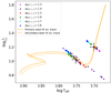 |
Fig. A.1. Position of the ten best models for the spectroscopic case for different choices of alpha concerning the observations, with the observational values including error bars given as black triangles. The evolutionary tracks of the primary and secondary for the best-fitting case are given in (dashed) orange lines. These two evolutionary tracks correspond to models with αMLT = 1.5, Z = 0.004 and masses of M1 = 1.39 M⊙ and M = 1.37 M⊙. |
This set of values for αMLT is lower than the values suggested by, for example, Trampedach et al. (2014) for models with a similar mass at a similar evolutionary stage. However, Trampedach et al. (2014) assumed solar metallicity for all models, while our target has sub-solar metallicity. This difference in metallicity and the known degeneracy between αMLT and metallicity (Joyce & Tayar 2023) are a probable cause for the shift in αMLT between this work and the models from Trampedach et al. (2014). The analysis for the M67 red giants by Reyes et al. (2024) also supports this conclusion.
Appendix B: Details on modeling
B.1. GYRE example inlist
In Listing 1 we provide an example inlist for the computation of the individual frequencies of the models using GYRE.
&constants /
&model
model_type = ’EVOL’
file = ’profile100.data.FGONG’
file_format = ’FGONG’
/
&mode
l = 0
/
&osc
outer_bound = ’ISOTHERMAL’
/
&rot /
&num
diff_scheme = ’COLLOC_GL4’
/
&scan
grid_type = ’LINEAR’
freq_min = 1
freq_max = 3000
n_freq = 5000
freq_min_units = ’UHZ’
freq_max_units = ’UHZ’
/
&grid
w_osc = 2
w_exp = 1
w_ctr = 4
/
&ad_output
summary_file = ’summary100.h5’
summary_item_list = ’l,n_pg,n_p,n_g, &
freq, freq_units,E_norm, M_star, &
R_star, L_star’
freq_units = ’UHZ’
/
&nad_output /
B.2. MESA example inlist
In Listing 2, we show an example MESA inlist for a model with a mass of 1.39 M⊙, metallicity of Z = 0.01 and helium abundance of Y = 0.27. The parameters marked in the example as ’variable’ were varied from model to model according to the ranges and stepsizes described in Sect. 3 and summarized in Table 2. The remaining parameters were kept constant for all computed models. For concise distplay, some lines were broken with the Fortran line break &.
&star_job
history_columns_file = &
history_columns_list_path
show_log_description_at_start = .false.
create_pre_main_sequence_model = .true.
save_model_when_terminate = .true.
save_model_filename = ’RGB.mod’
required_termination_code_string &
= ’log_L_upper_limit’
color_num_files = 2
color_file_names(1) = ’lcb98cor.dat’
color_num_colors(1) = 11
color_num_files = 2
color_file_names(2) = colorfilepath
color_num_colors(2) = 17
pgstar_flag = .false.
pause_before_terminate = .false.
relax_to_this_tau_factor = 0.001
relax_tau_factor = .true.
/ ! end of star_job namelist
&eos
/ ! end of eos namelist
&kap
kap_file_prefix = ’gs98’
use_Type2_opacities = .true.
/ ! end of kap namelist
&controls
x_ctrl(1) = 6000d0 ! Teff treshold
x_ctrl(2) = 1d9 ! Age_treshold
x_ctrl(3) = 2d5 ! max_timestep_years
x_ctrl(4) = 1.44 ! mass treshold
log_L_upper_limit = 1.5d0 !
mixing_length_alpha = 1.5 ! variable
initial_mass = 1.39 ! variable
initial_z = 0.006 ! variable
initial_y = 0.27 ! variable
num_trace_history_values = 2
trace_history_value_name(1) = &
’rel_E_err’
trace_history_value_name(2) = &
’log_rel_run_E_err’
cool_wind_full_on_T = 9.99d9
hot_wind_full_on_T = 1d10
cool_wind_RGB_scheme = ’Reimers’
RGB_to_AGB_wind_switch = 1d-4
Reimers_scaling_factor = 0.2
varcontrol_target = 1d-3
delta_lgL_He_limit = 0.01d0
time_delta_coeff = 0.5
!mesh
mesh_delta_coeff = 1
mesh_min_dr_div_cs = -1
max_allowed_nz = 30000
use_other_mesh_delta_coeff_factor = &
.false.
!output
photo_interval = -1
profile_interval = 4
history_interval = 1
terminal_interval = 100
write_header_frequency = 50
atm_T_tau_opacity = ’varying’
atm_T_tau_relation = ’Eddington’
!overshooting
overshoot_scheme(1) = ’exponential’
overshoot_zone_type(1) = ’any’
overshoot_zone_loc(1) = ’any’
overshoot_bdy_loc(1) = ’any’
overshoot_f0(1) = 0.005
overshoot_f(1) = 0.02
max_num_profile_models = 10000
max_model_number = 50000
/ ! end of controls namelist
&pgstar
/ ! end of pgstar namelist
B.3. Investigation of temporal resolution in MESA and GYRE
As described in Sect. 5.2, adjusting the timesteps in MESA to provide sufficient input files for calculating Δν from with GYRE was necessary. The time_delta_coeff was set to 0.5, half of its default value for all model runs. This was sufficient to have small enough parameter steps in Teff and logg not to exceed the respective observational uncertainties. However, the steps in Δν were still orders of magnitudes above the observational uncertainty of 0.03 μHz. To solve this problem, we needed to find the right trade-off between a small enough timestep to get this desired resolution but not too small to become numerically unstable and require excessive computation time. This trial and error search resulted in a maximum allowed timestep in MESA of 0.2 Myr enforced from the subgiant branch onward for models cooler than 6000 K. The differential variations for spectroscopic parameters and Δν for an exemplary model of 1.39 M⊙ and Z = 0.007 enforcing the condition mentioned above is shown in Fig. B.1. While this method works fine for stars up to around 1.44 M⊙, the differential stepsizes in Δν increase for masses above it. We therefore implemented another threshold at 1.44 M⊙, where a maximal step size of 0.1 Myr was enforced. The necessary modifications in the runstarextra file are shown in Listing 3, while the thresholds described above were defined in the respective MESA inlists.
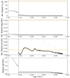 |
Fig. B.1. Variation of the parameters used in the figure of merit between consecutive time steps of a model for a star with 1.39 M⊙ and Z = 0.007. The top, middle, and bottom panels show the differential evolution of the effective temperature Teff, surface gravity logg and Δν, respectively. The vertical gray line indicates when a maximum timestep of 0.2 Myr was enforced between two models. The horizontal orange lines indicate the respective observational uncertainties for the given parameters. The bottom panel gives the timestep between consecutive models as a function of age. |
integer function extras_finish_step(id)
use chem_def
integer, intent(in)::id
integer::ierr
real(dp)::Teff_treshold
real(dp)::Age_treshold
real(dp)::max_timestep_years
real(dp)::mass_treshold
type (star_info), pointer::s
ierr = 0
call star_ptr(id, s, ierr)
if (ierr /= 0) return
extras_finish_step = keep_going
Teff_treshold = s% x_ctrl(1)
Age_treshold = s% x_ctrl(2)
max_timestep_years = s% x_ctrl(3)
mass_treshold = s% x_ctrl(4)
s% xtra(1) = s% Teff
if ((s% xtra(1) < Teff_treshold) &
.AND. (s% star_age > Age_treshold)) then
s% need_to_update_history_now = .true.
s% need_to_save_profiles_now = .true.
s% max_years_for_timestep = &
max_timestep_years
endif
if ((s% initial_mass & +
.GE. mass_treshold)) then
s% max_years_for_timestep = &
max_timestep_years/2
endif
end function extras_finish_step
All Tables
Cases considered for modeling KIC 9163796 and the associated stellar parameters determined from χred2-minimization.
All Figures
|
Fig. 1. Hertzsprung-Russel diagram depicting the positions of the primary (upward triangle) and secondary (downward triangle) component of KIC 9163796 according to the asteroseismic analysis from Beck et al. (2018). As references, the tracks of a 1 M⊙, 1.4 M⊙, and 2 M⊙ evolutionary track with the primary’s metallicity from MESA are provided as dashed lines. The background contour plot shows the density distribution of all targets from the input catalogs used in Beck et al. (2024), Mathur et al. (2022) with an asteroseismic detection. |
| In the text | |
|
Fig. 2. Comparison of the best-fitting solutions for case A regarding the treatment of metallicity. The gray solutions have the metallicity varying freely in the modeled range (Case A0), the magenta solution only allows values where the metallicity of the primary equals the metallicity of the secondary (Case A1), while the royal blue solutions force both metallicities to be equal to the spectroscopic solution (Case A2). The cyan part only allows values in the range of 1σ around the spectroscopic value (Case A3). The magenta triangle, blue cross, and gray dot mark the respective minima of the corresponding datasets. The dashed horizontal line shows where χred2 = 1. |
| In the text | |
|
Fig. 3. Secondary mass and χred2-minima as a function of primary mass from the models with the condition of equal metallicity for the components Z1 = Z2 (Case A1). The color bar indicates the respective χred2-minima on a logarithmic scale. The residuals were calculated with enforcing M1 ≥ M2; the gray area represents the respective space where no χred2 is calculated due to this condition. The seismic solution, including its error bars from BKP18, is given in black, the absolute χred2-minimum is given in magenta triangle, and the green line represents the spectroscopic mass ratio of q = 1.015. |
| In the text | |
|
Fig. 4. Comparison of the best-fitting solutions regarding the treatment of metallicity for the case of including νmax in the figure of merit (Case B). The magenta solution only allows values where the metallicity of the primary equals the metallicity of the secondary (Case B1), while the royal blue solutions force both metallicities to be equal to the spectroscopic solution (Case B2). The cyan part only allows values in the range of 1σ around the spectroscopic value (Case B3). Symbols and colors are identical to Fig. 2. |
| In the text | |
|
Fig. 5. Comparison of the best-fitting solutions regarding the treatment of metallicity, with the figure of merit used including the local Δν and νmax of the primary in the figure of merit (Case C). The magenta solution only allows values where the metallicity of the primary equals the metallicity of the secondary (Case C1), while the royal blue solutions force both metallicities to be equal to the spectroscopic solution (Case C2). The cyan part only allows values in the range of 1σ around the spectroscopic value (Case C3). Symbols and colors are identical to Fig. 2. |
| In the text | |
|
Fig. 6. Residuals of the χred2-minimization as a function of the primary mass M1 and secondary mass M2 with the condition of equal metallicity within the uncertainty range of the spectroscopic value of the components Z1, 2 = Zspec ± σZspec (Case C3), with the inclusion of Δν in the figure of merit. Colors and symbols are the same as in Fig. 3. We added the revised seismic masses obtained from the corrected Δν value as an orange cross. |
| In the text | |
|
Fig. 7. Comparison of the best-fitting solutions regarding the treatment of metallicity for the case that includes the local Δν of the primary and the magnitude difference of the components in the figure of merit (Case D). The magenta solution only allows values where the metallicity of the primary equals the metallicity of the secondary (Case D1), while the royal blue solutions force both metallicities to be equal to the spectroscopic solution (Case D2). The cyan part only allows values in the range of 1σ around the spectroscopic value (Case D3). Symbols and colors are identical to Fig. 2. |
| In the text | |
|
Fig. 8. Residuals of the χred2-minimization as a function of the primary mass M1 and secondary mass M2 with the condition of equal metallicity within the uncertainty range of the spectroscopic value of the components Z1, 2 = Zspec ± σZspec (Case D3); with the inclusion of Δν and the magnitude difference Δm in the figure of merit. Colors and symbols are the same as in Fig. 3. We added the revised seismic masses obtained from the corrected Δν value as an orange cross. |
| In the text | |
|
Fig. 9. Residuals of χred2-minimization in the mass-initial helium plane for both components (primary left, secondary right) for case D3. The best-fitting solution for each is marked as a magenta triangle. |
| In the text | |
|
Fig. 10. Residuals of the χred2-minimization in the mass-metallicity plane for both components (primary left, secondary right) for identical metallicities for both components (Case D1). For this case, the magenta triangle marks the best-fitting solution. For the analogous case, with both model metallicities forced to be in the 1-σ-uncertainty of the spectroscopic value (Case D3), the best fitting solution is given as a blue cross. The dashed lines show the 1σ-errorbar around the spectroscopic metallicity. |
| In the text | |
|
Fig. 11. Age estimations for the different cases of the figure of merit, including their uncertainties. The cases are calculated as described in Sect. 4, with the cases color coded as follows: magenta: Z1 = Z2; royal blue: Z1, 2 = Zspec; cyan: Z1, 2 = Zspec ± σZspec. |
| In the text | |
|
Fig. 12. Mass estimations for the primary for different cases of the figure of merit, including their uncertainties. The color coding is the same as in Fig. 11. The black solid line indicates the revised mass estimation from observations, with the gray area indicating the respective 1-σ error. The gray dashed line indicates the mass as given in BKP18. |
| In the text | |
|
Fig. A.1. Position of the ten best models for the spectroscopic case for different choices of alpha concerning the observations, with the observational values including error bars given as black triangles. The evolutionary tracks of the primary and secondary for the best-fitting case are given in (dashed) orange lines. These two evolutionary tracks correspond to models with αMLT = 1.5, Z = 0.004 and masses of M1 = 1.39 M⊙ and M = 1.37 M⊙. |
| In the text | |
|
Fig. B.1. Variation of the parameters used in the figure of merit between consecutive time steps of a model for a star with 1.39 M⊙ and Z = 0.007. The top, middle, and bottom panels show the differential evolution of the effective temperature Teff, surface gravity logg and Δν, respectively. The vertical gray line indicates when a maximum timestep of 0.2 Myr was enforced between two models. The horizontal orange lines indicate the respective observational uncertainties for the given parameters. The bottom panel gives the timestep between consecutive models as a function of age. |
| In the text | |
Current usage metrics show cumulative count of Article Views (full-text article views including HTML views, PDF and ePub downloads, according to the available data) and Abstracts Views on Vision4Press platform.
Data correspond to usage on the plateform after 2015. The current usage metrics is available 48-96 hours after online publication and is updated daily on week days.
Initial download of the metrics may take a while.