| Issue |
A&A
Volume 697, May 2025
|
|
|---|---|---|
| Article Number | A135 | |
| Number of page(s) | 29 | |
| Section | Galactic structure, stellar clusters and populations | |
| DOI | https://doi.org/10.1051/0004-6361/202453024 | |
| Published online | 19 May 2025 | |
Linking photometry and spectroscopy: profiling multiple populations in globular clusters
1
Istituto Nazionale di Astrofisica – Osservatorio Astronomico di Padova,
Vicolo dell’Osservatorio 5,
Padova
35122,
Italy
2
Dipartimento di Fisica e Astronomia “Galileo Galilei”, Univ. di Padova,
Vicolo dell’Osservatorio 3,
Padova
35122,
Italy
3
Center for Galaxy Evolution Research and Department of Astronomy, Yonsei University,
Seoul
03722,
Republic of Korea
4
INAF – Osservatorio Astronomico di Roma,
Via Frascati 33,
00040
Monte Porzio Catone, Roma,
Italy
5
Research School of Astronomy and Astrophysics, Australian National University,
Canberra,
ACT 2611,
Australia
6
South-Western Institute for Astronomy Research, Yunnan University,
Kunming
650500,
PR
China
★ Corresponding author; emanuele.dondoglio@inaf.it
Received:
15
November
2024
Accepted:
18
March
2025
Our understanding of multiple populations in globular clusters (GCs) largely comes from photometry and spectroscopy. Appropriate photometric diagrams are able to disentangle first and second populations (1P and 2P, respectively), with 1P having chemical signatures similar to field stars and 2P stars showing unique light-element variations. Spectroscopy enables detailed analysis of chemical abundances in these populations. We combined multi-band photometry with extensive spectroscopic data to investigate the chemical composition of multiple populations across 38 GCs, yielding a chemical abundance dataset for stars with precise population tagging. This dataset provides the most extensive analysis to date on C, N, O, Na, Mg, and Al variations, revealing the largest sample of light-element spreads across GCs. We find that GC mass correlates with light-element variations, which supports earlier photometric studies. We investigated iron differences among 1P stars, confirming their presence in 19 GCs, and finding a spread consistent with prediction based on photometry. Notably, in eight GCs we detected a clear correlation between [Fe/H] values and their position in iron-sensitive photometric diagrams. More massive GCs display larger lithium depletion among 2P stars, which is consistent with zero at smaller masses. Some 2P stars, despite their extreme chemical differences from 1P stars, exhibit lithium abundances similar to those of 1P stars. This suggests that the polluters responsible for the 1P population have produced lithium. We analyzed anomalous stars in 10 GCs. These stars are characterized by enrichment in iron, s-process elements, and C+N+O. NGC 1851, NGC 5139 (ωCen), NGC 6656, and NGC 6715 display light-element inhomogeneities similar to 1P and 2P stars. Iron and barium enrichment varies widely, being negligible in some clusters and much larger than observational errors in others. Generally, these elemental spreads correlate with GC mass. In clusters with available data, anomalous stars show C+N+O enrichment compared to the non-anomalous stars.
Key words: techniques: photometric / stars: abundances / stars: Population II / globular clusters: general
© The Authors 2025
 Open Access article, published by EDP Sciences, under the terms of the Creative Commons Attribution License (https://creativecommons.org/licenses/by/4.0), which permits unrestricted use, distribution, and reproduction in any medium, provided the original work is properly cited.
This article is published in open access under the Subscribe to Open model. Subscribe to A&A to support open access publication.
1 Introduction
The origin of multiple stellar populations in globular clusters (GCs) remains an unsolved astrophysical puzzle. In recent years, our understanding of the observational properties associated with diverse stellar populations has significantly increased, largely due to the contribution of spectroscopic and photometric techniques. However, the mechanisms responsible for the formation of these populations remain unclear (see Bastian & Lardo 2018; Gratton et al. 2019; Milone & Marino 2022, for the most recent reviews on the phenomenon).
The multiple-color plots, now nicknamed “chromosome maps” (ChMs), were originally introduced based on a combination of four Hubble Space Telescope (HST) bands (F275W, F336W, F438W and F814W). This combination allows for the construction of a plane in which the position of stars is sensitive to the chemical abundance of elements involved in high-temperature H-burning, via the molecules that they form, and to the helium and iron abundances. The analysis of these maps has enabled us to define the main properties of the multiple population phenomenon as follows:
At least two groups of stars, called first and second populations (1P and 2P, respectively), can be distinguished along the maps. The chemical abundances of 1P stars are similar to Halo field stars, whereas 2P stars are O- and C-depleted and enhanced in He, N, Na, and Al (Marino et al. 2008; Carretta et al. 2009; Milone et al. 2012; Lee & Sneden 2021; Lee 2022).Both 1P and 2P stars trace the typical ChM sequence observed in most Milky Way GCs, named Type I clusters.
More massive clusters exhibit higher fractions of 2P stars (e.g., Milone et al. 2017; Lagioia et al. 2025) and host He-enhanced 2P stars, which generally show more extreme chemical differences.
For the majority of the Galactic GCs studied, the fraction of 2P stars generally exceeds the 1P fraction.
The 1P group itself is not chemically homogeneous, showing a sizable spread in the mF275W − mF814W color (e.g., Milone et al. 2017; Dondoglio et al. 2021), which corresponds to the x-axis of the ChMs. Spectroscopic and photometric analyses suggest that relatively small variations in overall metal content are responsible for this spread (Legnardi et al. 2022; Lardo et al. 2022; Marino et al. 2023).
A significant fraction of GCs (almost 20%) show peculiar ChMs. These clusters, classified as Type II, display additional sequences running parallel to the main 1P/2P stream of the ChM. These sequences are often referred to as anomalous stars and comprise stellar populations with enhanced metals and, in most cases, abundances of s-process elements and total C+N+O content (see Carretta et al. 2011; Marino et al. 2015; Yong et al. 2015; Milone et al. 2017; McKenzie et al. 2022; Dondoglio et al. 2023).
Using spectroscopic elemental abundances from the literature, Marino et al. (2019a) explored the chemical content of stellar populations observed along the ChM of 29 GCs. This analysis shows that stars with different abundances of light elements populate distinct regions of the ChM. However, despite spanning a broad color range on the map, 1P stars exhibit uniform chemical abundances (relative to iron) for the same elements. Because the ChMs were available only in relatively small fields of view of the HST cameras, chemical tagging on ChMs has so far been restricted to stars located in the most central regions of the GCs.
Recently, Jang et al. (2022) constructed ChMs using groundbased UBVI photometry, providing stellar population identifications based on maps for larger fields of view. The availability of maps for larger regions across the clusters allows for the investigation of chemical and spatial properties of the multiple populations extending to the outermost cluster regions. These outer regions could retain the fossil configuration of the system at the epoch of formation (e.g., Mastrobuono-Battisti & Perets 2016).
In this study, we used the two sets of ChMs published by Milone et al. (2017) and Jang et al. (2022) based on HST and ground-based photometry, respectively, with the new ChMs introduced in this work. We combined this information with spectroscopic abundances from the literature to explore the chemical patterns of multiple stellar populations. Our dataset comprises 38 GCs, in which approximately 3200 stars have chemical abundances in at least one of the 14 chemical species considered in this work, namely A(Li), [C/Fe], [N/Fe], [O/Fe], [Na/Fe], [Mg/Fe], [Al/Fe], [Si/Fe], [K/Fe], [Ca/Fe], [Ti/Fe], [Fe/H], [Ni/Fe], and [Ba/Fe]. The paper is organized as follows. Section 2 presents the whole dataset exploited in this work, including both photometry and spectroscopy; Section 3 illustrates the chemical composition of 1P and 2P stars among our sample of GCs; Section 4 investigates the spread in different elements and its relation with cluster mass and metallicity; Section 5 focuses on the presence of iron variations among 1P stars; Section 6 studies lithium depletion among 2P stars; and Section 7 provides a detailed analysis of the anomalous population of Type II GCs. Finally, a summary and conclusions from our work are reported in Section 8.
2 Dataset
2.1 Photometric dataset
In this work, we utilized multi-facility photometry to identify the multiple populations hosted by GCs. In particular, we employ the following two collections of published ChMs:
HST ChMs from Milone et al. (2017). In this work, Milone and collaborators combined HST ultraviolet (UV) and optical photometry from the UV and visual channel of the Wide Field Camera 3 (WFC3/UVIS) and the Advanced Camera for Survey (WFC/ACS), using the F275W, F336W, and F438W and F814W filters, from multiple programs (see their Section 2). The published ChMs allowed for a clear-cut separation between 1P and 2P stars among red-giant branch (RGB) stars of 57 Galactic GCs. The HST fields of view exploited in this work cover the innermost ~2.7 arcmin, providing an effective separation in their central areas. Furthermore, we used the ChMs of NGC 2419 and NGC 6402 published by Zennaro et al. (2019) and D’Antona et al. (2022), respectively, obtained through the same procedure.
Ground-based ChMs from Jang et al. (2022). This study exploited the photometric dataset published by Stetson et al. (2019), which produced UBVRI catalogs of 48 Milky Way GCs based on a large sample of ground-based archive observations taken with various facilities. Jang and colleagues utilized this dataset to build ChMs for 29 GCs, for which a separation between the distinct stellar groups is possible along the RGB. These ChMs are based on observations over a wider field of view than those of the HST, thus providing a multiple population tagging up to around the outskirts of the GCs.
Moreover, we considered the U-band Wide-Field Imager (WFI) photometry of NGC 5286 and NGC 6656 from the SUrvey of Multiple pOpulations in GCs (SUMO; program 088.A-9012-A, PI. A. F. Marino), taken with the Max Planck 2.2 m telescope at La Silla (e.g., Marino et al. 2015, 2019a). This photometry, combined with archive observations in the B, V, and I bands, allowed us to build ground-based ChMs for these two GCs. Finally, we used the NGC,5139 (ωCen) catalog recently published by Häberle et al. (2024). This dataset was built by uniform reduction of all archival HST images in the innermost 10 × 10 arcmin2, which allowed us to build a ChM to separate multiple populations at larger distances than was possible considering the ChM by Milone et al. (2017) alone. The ChMs that we introduce in this study are presented in Section 3.1.
2.2 Spectroscopic dataset
To estimate the chemical properties of the multiple populations detectable from the ChM, stars with available chemical abundances were cross-matched with the diagrams described in Section 2.1. This allowed us to explore the chemical properties of each population identified through photometry. We considered the following elements in our study: Li, C, N, O, Na, Mg, Al, Si, K, Ca, Ti, Fe, Ni, and Ba. Our analysis incorporates data from three spectroscopic surveys:
Apache Point Observatory Galactic Evolution Experiment (APOGEE). This survey, conducted utilizing the du Pont Telescope and the Sloan Foundation 2.5 m Telescope (Gunn et al. 2006) at Apache Point Observatory, observed over 700 000 stars with a resolution of R ~ 22 500. The latest Data Release 17 (DR17, Abdurro’ uf et al. 2022) offers chemical abundance insights into multiple populations of 21 GCs in our sample, making it the most extensive dataset of stars that overlap with our photometric sample. We selected APOGEE stars with a signal-to-noise ratio (S/N) > 70 and excluded those flagged with ASCAPFLAG set to STAR_BAD, indicative of spectrum-related issues such as a high number of bad pixels or non-stellar classification1. The APOGEE dataset provides two carbon abundances, C and CI, measured through molecules and neutral carbon lines, respectively. Jönsson et al. (2020) proved that for metal-poor stars, the CI is likely to be more accurate because molecular lines become particularly weak. For this reason, we consider the CI values as a tracer of the carbon abundances in our sample. Jönsson et al. (2020) have also shown that APOGEE [Na/Fe] measurements rely on relatively weak lines, making this element one of the least reliable of this survey. Because sodium has been extensively studied in the literature, we do not consider [Na/Fe] estimates based on APOGEE spectra because of their relatively poor reliability.
Gaia-ESO Survey (GES). This survey utilizes spectroscopy data obtained from the FLAMES (Fibre Large Array Multi Element Spectrograph) spectrograph (Pasquini et al. 2002) on the Very Large Telescope (VLT), operating in multi-object spectroscopy mode with GIRAFFE and UVES (Ultraviolet and Visual Echelle Spectrograph), with spectral resolutions of R ~ 18 000–35 500 (depending on the setup) and ~47 000, respectively. The latest internal Data Release 6 (iDR6; see Gilmore et al. 2022; Randich et al. 2022; Hourihane et al. 2023) covers data from more than 114000 stars, including members of 11 GCs featured in our sample. Abundance selection criteria involve simplified flags2: SNR, to exclude stars with inaccurate results caused by a low signal-to-noise ratio; SRP, to avoid stars with spectral reduction problems and no available abundances; and NIA, that excludes sources with too few available lines for abundance determinations.
Galactic Archaeology with HERMES (GALAH). This initiative derives chemical abundances using the High Efficiency and Resolution Multi-Element Spectrograph (HERMES) at the Anglo-Australian Telescope (Sheinis et al. 2015), achieving a resolution of R ~ 28 000. Our analysis used the most recent Data Release 4 (GALAH+DR4, see Buder et al. 2024), which includes data from more than 900 000 Milky Way stars. We identified RGB stars with ChM tagging in nine GCs. The selection process for the stellar sample adhered to the criteria recommended in the GALAH+DR4 documentation3, including SNR > 30, flag_sp == 0, and flag_x_fe == 0.
As a general criterion, in addition to the specific ones listed for each survey, we also excluded abundance measurements characterized by uncertainties much larger than their average values.
Finally, we extensively used 56 publicly available spectroscopic catalogs from studies published within the last ~20 years. These catalogs contain abundance measurements for elements relevant to our study, as listed in Table A.1.
In the following analysis, we only considered abundance ratio measurements, excluding upper limits. Among the datasets considered, upper limits were present for A(Li), [O/Fe], [Na/Fe], and [Al/Fe].
2.3 Final dataset
This study focused on GC stars with both population tagging from the ChM and available spectroscopic abundances. Our final sample included 38 GCs, of which 37 (all except NGC 1904) have available HST ChM, 23 have ground-based ChM, and 22 have both available.
Detailed information on the selected GCs, the public catalogs used, and the number of common stars for each element is presented in Table A.1. The numbers provided represent the combined count of 1P and 2P stars with spectroscopic abundance data. Notably, for Type II GCs (namely NGC 0362, NGC 1261, NGC 1851, NGC 5139, NGC 5286, NGC 6388, NGC 6656, NGC 6715, NGC 6934, and NGC 7089), this count also includes the anomalous population. Our final sample of stars with both ChM and chemical abundance information comprised 1004 1P stars, 1883 2P stars, and 303 anomalous stars. In total, our sample consisted of 3190 cluster members.
3 Chemical abundances of multiple stellar populations
We combined population tagging from HST- and ground-based ChMs with spectroscopic measurements from the literature to assess the chemical abundances of various populations within GCs. Section 3.1 involves the identification of 1P and 2P stars (including the anomalous stars when present) in the ChM. In Section 3.2, we combined this selection with our spectroscopic dataset to determine the median values and variability in the chemical abundances of the tagged populations.
3.1 Population tagging along the Chromosome Map
The first step in determining the chemical characteristics of multiple stellar populations involved a precise selection process within the ChM. To accomplish this, we employed the methodology outlined by Dondoglio et al. (2023) to distinguish various populations within the ChM of NGC 1851. This approach involved constructing ellipses to enclose the blobs of stars representing distinct groups, using the following three steps. First, we visually identified genuine 1P and 2P members and used the median of the ChM coordinates as their center. Secondly, we determined the optimal orientation that minimizes their orthogonal dispersion to establish the major axis orientation of the ellipses. Thirdly, we derived the lengths of the semi-major and semi-minor axes by considering 2.5 times the dispersion of the stars along their respective directions determined in the preceding step. We considered anomalous stars to be those selected by Milone et al. (2017) and Jang et al. (2022), based on their position in the mF336W vs. mF336W–mF814W and I vs. U–I color magnitude diagrams (CMDs), respectively4. The anomalous GCs NGC 6715 and NGC 7089 host an additional population (see Milone et al. 2017, and references therein). For NGC 6715, this population has been associated with the host Sagittarius dwarf galaxy (e.g., Siegel et al. 2007). For NGC 7089, these stars likely have a similar origin (e.g., Milone et al. 2015). We have not included them among the anomalous stars. We considered them as a separate population from the other GC populations in the case of NGC 7089, while for NGC 6715 no spectroscopic measurements are available for the stars in the ChM. For the ground-based catalogs of NGC 5286 and NGC 6656, we relied on the anomalous star tagging performed by Marino et al. (2019a).
An example of the results of our cross-matching is shown in Figure 1. The left panels display the HST ChMs of NGC 5904 and NGC 1851, which are Type I and II GCs, respectively. The two right panels represent the same tagging, using ground-based ChMs. Stars with available spectroscopic measurements in at least one of the datasets reported in Table A.1 are colored green, violet, and red according to whether they belong to the 1P, 2P, or anomalous populations, respectively. If a star has population tagging in both ChMs, we considered the photometric information from the HST data. In Appendix A, we display all the ChMs published by Milone et al. (2017) and Jang et al. (2022) for the clusters in our sample, where the stars with available spectroscopy are color coded following the designations introduced in Figure 1.
As discussed in Section 2, we also considered additional photometric diagrams, which are summarized in Figure 2. Panels (a1) and (a2) display the diagrams used to distinguish 1P and 2P stars in the red Horizontal Branch (HB) of NGC 5927, based on HST photometry and UBI photometry, respectively. Since no spectroscopic measurements of RGB stars with ChM tagging are documented in the literature, we focused on the red HB evolutionary phase, which has been examined in the context of chemical abundance analysis. Dondoglio et al. (2021) demonstrate the effectiveness of HST and ground-based multi-band photometry in distinguishing 1P and 2P stars among red HB stars, using the mF275W–mF336W vs. mF336W–mF438W two-color diagram presented in panel (a1), where 1P stars occupy the lower-left sequence, and the pseudo-two-color diagram CU,B,I vs. B − I in panel (a2), in which 1P and 2P stars are distributed below and above CU,B,I ~ −1.7, respectively. We then built the ground-based ChMs of NGC 5286 (panel (b)) and NGC 6656 (panel (c)) by following the same approach of Jang et al. (2022), considering the U-B color and the CU,B,I pseudo-color from the datasets presented in Section 2.1. Finally, ΔCF275W,F336W,F435W vs. ΔF275W,F814W ChM of ωCen derived from the Häberle et al. (2024) catalog is presented in panel (d), obtained by applying the iterative procedure introduced in Appendix A of Milone et al. (2017). This diagram was used to tag populations among stars outside ~2 arcmin from the cluster center, while for the innermost area we considered the ChM by Milone and collaborators. In all these diagrams, stars with available chemical abundances are depicted as in Figure 1.
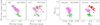 |
Fig. 1 Left panels: from left to right, ΔCF275W,F336W,F438W vs. ΔF275W,F814W HST ChMs of NGC 5904 and NGC 1851. 1P, 2P, and anomalous stars with available spectroscopy measurements are highlighted with green, violet, and red dots, respectively. Right panels: as per left panels but with the ground-based ΔCU,B,I vs. ΔB,I ChM. |
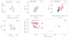 |
Fig. 2 Summary of the photometric diagrams introduced in Section 3.1. Panel (a1) and (a2): two-color diagram of mF275W-mF336W vs. mF336W-mF438W and CU,B,I vs. B − I pseudo two-color diagram for the red HB of NGC 5927. Panel (b): ΔCU,B,I vs. ΔU,B ChM of NGC 5286. Panel (c): same but for NGC 6656. Panel (d): ΔCF275W,F336W,F435W vs. ΔF275W,F814W ChM of ωCen derived from the catalog by Häberle et al. (2024). Green, violet, and red dots represent 1P, 2P, and anomalous stars, respectively. |
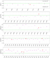 |
Fig. 3 Differences in median abundances of A(Li), [C/Fe], [N/Fe], [O/Fe], and [Na/Fe] between 1P and 2P stars (violet) and 1P and anomalous (red) stars. The green lines separate the regime where 2P and anomalous stars are enriched or depleted (see text for details). The y-axis scale is adjusted in each plot to optimize clarity. The smaller dots indicate GCs where the Δ[C/Fe] and Δ[N/Fe] measurements are derived from RGB stars brighter than the bump. |
3.2 Element abundances and distribution
Next, we investigate the presence of chemical differences among the different populations in our sample of GCs. The results for A(Li) [C/Fe], [N/Fe], [O/Fe], and [Na/Fe] are shown in Figure 3, while Figure 4 illustrates [Mg/Fe], [Al/Fe], and [Si/Fe], [K/Fe], and [Ca/Fe], and Figure 5 [Ti/Fe], [Fe/H], [Ni/Fe], and [Ba/Fe]. The spectral features analyzed in the considered works cover two wavelength regimes: the optical range, which covers approximately 3500–8800 Å, and the IR regime exploited by APOGEE, which covers the H band (1.15–1.70 μm). In each plot, the y-axis shows the ΔX quantity, where X is any of the considered elemental ratios, measured as the difference between the median abundance of 2P stars (violet points) or anomalous stars (red points) and the 1P stars. The values relative to the population in NGC 7089 associated with the remnant of its host galaxy are represented by orange stars. The positive and negative values of ΔX indicate that 2P (or anomalous) stars are enriched and depleted, respectively, in a given element compared to the 1P population, as shown in the upper panel of Figure 3. The horizontal green line delimits the two regimes and, by definition, is positioned at ΔX = 0.ΔX has been measured only by considering the datasets with at least four 1P, four 2P, and (when present) four anomalous stars, to ensure sufficient statistics for deriving reliable median abundances of each population. As NGC 5986, NGC 6388, and NGC 6934 do not meet these criteria for any of the elements involved, they do not appear in the analysis presented in the current section. However, we still include them in our dataset, as they were involved in the analysis of Sections 4 and 7.
In Table A.3, we display all ΔX along with their uncertainties, which were derived by propagating the 1P, 2P and anomalous median abundance errors. These errors were estimated as r.m.s. (root mean square) / ![$\[\sqrt{N-1}\]$](/articles/aa/full_html/2025/05/aa53024-24/aa53024-24-eq1.png) , with N being the number of stars of a certain population.
, with N being the number of stars of a certain population.
For GCs with abundances from more than one dataset in a given element, we separately measured ΔX for each dataset, and then combined them by considering their weighted average5.
Using the results presented in Figures 3, 4, and 5, in addition to Table A.3, we discuss the trends for each element individually.
Lithium. We considered A(Li) abundances only for stars below the RGB bump, as brighter stars experience extra mixing that leads to a decreasing trend in lithium abundance with magnitude, which may introduce a bias in the relative behavior of the different populations6. All lithium measurements in the studies considered exploited lines in the Li I doublet at ~6708 Å. Visual inspection of Figure 3 revealed a slight decrease among 2P stars, with the exception of NGC 6656, NGC 6809 and NGC 6838. Overall, ΔA(Li) spans a range from ~0.0 to ~−0.2 dex. In NGC 6656, the anomalous population has an A(Li) distribution similar to 2P stars. Section 6 contains a detailed investigation of the lithium distribution among multiple populations.
Carbon. The [C/Fe] measurements in this study are based on the CH and CH G bands in the 3800–4200 Å range, the CI line at ~6588 Å, and the CI lines in the H-band. The extra mixing after the first dredge-up affects not only lithium, but also the abundances of carbon and nitrogen (e.g., Charbonnel et al. 1998; Shetrone et al. 2019; Lee 2023), causing a decrease in carbon and an increase in nitrogen, both dependent on magnitude. For this reason, for stars below the RBG bump, results based on [C/Fe] and [N/Fe] abundances are generally more reliable. Measurements of Δ[C/Fe] for stars based below the bump were only possible for nine GCs. These values tend to exhibit negative values or are consistent with zero (e.g., NGC 5272, NGC 6254, and NGC 6656), indicating that, as expected, 2P stars generally have lower carbon abundances than 1P stars. Conversely, the anomalous population of NGC 6656 is significantly richer in carbon than its 1P stars. In Figure 3, smaller dots denote the Δ[C/Fe] based on stars brighter than the RGB bump. Although these estimates are generally less reliable due to their dependence on magnitude, we highlight how their values qualitatively agree with a carbon depletion in 2P stars. Moreover, anomalous stars in NGC 1851 appear to be, on average, more carbon-poor than 2P stars.
Nitrogen. [N/Fe] were obtained by exploiting the CN absorption bands (once known C) present in both the optical and H-band ranges. We represent Δ[N/Fe] following the same approach adopted for carbon, as this element is also affected by extra mixing. We illustrated the measurements for stars below and above the RGB bump using larger and smaller dots, respectively. Here, all the clusters have positive values (i.e., are N-enhanced), ranging from approximately 0.3–0.9 dex. Nitrogen displays one of the largest elemental variations between 1P and 2P stars. Anomalous stars in both NGC 1851 and NGC 6656 exhibit larger median [N/Fe] values than their 2P stars.
Oxygen. The considered studies measured oxygen abundance using the forbidden [O I] lines (6300 and 6364 Å) and the oxygen triplet around 7770 Å in the optical region, as well as the NIR OH absorption bands for APOGEE data. The Δ[O/Fe] values are consistent with a depletion among 2P stars in almost all studied clusters, with the exception of NGC 0362, NGC 4590, and NGC 6535 where they are negligible. Values range from approximately −0.05 to −0.35 dex, with the remarkable exception of NGC 6402, which exhibits a significant depletion of ~−0.8 dex. Anomalous stars in NGC 1851 display smaller [O/Fe] compared to 2P stars, while in NGC 5139 and NGC 6656 they span similar ranges.
Sodium. All [Na/Fe] estimates were obtained through the sodium doublets at 5682–5688 Å and 6154–6160 Å. Similar to nitrogen, 2P stars exhibit an overall enhancement in this element, with only NGC 4590, NGC 5024, and NGC 5286 displaying a negligible Δ[Na/Fe] within uncertainties. NGC 6402 exhibits the largest enhancement, with a value of ~0.6 dex.
Magnesium. Magnesium abundances were derived using several Mg I lines in the 5300–8800 Å range (primarily the 5711 Å line), as well as lines in the H band. Figure 4 illustrates that magnesium differences are very small, with 8 of the 27 studied GCs being consistent with zero within the uncertainty. In only one case, NGC 6715, Δ[Mg/Fe] lies above the green line, while in the rest of our sample we detected a modest but significant depletion (≲0.2 dex) among 2P stars, as previously suggested in the literature (e.g., Carretta 2015; Pancino et al. 2017). NGC 2419 stands out as a notable outlier, with a much larger depletion of ~−0.9 dex. Anomalous stars generally exhibit similar behavior to 2P stars, with the exception of ωCen, which displays a smaller average magnesium abundance. Stars in the NGC 7089 host galaxy have average [Mg/Fe] closer to 2P stars, even though the large uncertainty resulting from a sample of only four stars prevents us from excluding 1P-like abundances.
Aluminum. Aluminum was primarily measured through doublets in the 6700–8800 Å range and by exploiting Al features in H band. [Al/Fe] spans the largest abundance interval, ranging from a negligible difference (e.g., NGC 5927 and NGC 6121), up to a ~1 dex enhancement, for NGC 6205 and NGC 6254. Anomalous stars in NGC 1851 and NGC 5139 are the most Al-rich stars in their host GCs, while in NGC 6656 they cover a similar range to 2P stars.
Silicon. We found no evident [Si/Fe] trend between populations from inspecting the distributions shown in Figure 4. Values for Δ[Si/Fe] were around zero, ranging from 0.12 to −0.06 dex. Notably, a small but significant depletion of silicon in 2P stars was observed in NGC 0104, NGC 1851, ωCen, NGC 6254, and NGC 6838, while NGC 6809 and NGC 7078 exhibit a modest enhancement. Anomalous stars in NGC 1851 and ωCen show a similar depletion to 2P stars, while in NGC 6656 they are slightly more Si-rich than 1P stars. Stars in NGC 7089’s host galaxy exhibited average silicon abundances consistent with those of the cluster stars.
Potassium. Measurements of [K/Fe] were taken from the K resonance line at ~7699 Å in the optical regime, and from different K I lines (such as those at 15 163 and 15 168 Å) in the H band. No clear overall trends in potassium variation are apparent in Figure 4. Although Δ[K/Fe] spans a range from ~−0.15 to ~0.10, its large errors (due to a relatively small sample of stars with these measurements) prevent us from detecting any significant difference. Cases with significant K-enhancement are NGC 0104, NGC 6752, and the remarkable NGC 2419, which exhibits a very high (~0.9 dex) enhancement among 2P stars. In contrast, 2P stars of NGC6838 are modestly depleted in potassium. Finally, anomalous stars in ωCen are significantly K-richer than the 1P stars.
Calcium. Overall, no particular trend was observed in the values of Δ[Ca/Fe]. From the values reported in Table A.3, we note a small Ca-depletion among the 2P stars of NGC 1904, NGC 5286, NGC 6752, NGC 6809, NGC 7078, and NGC 7089, and Ca-enhancement in NGC 0362, NGC 1851, NGC 2419, and NGC 6402, all significant at a 1-σ level. Anomalous stars in NGC 1851 are slightly more Ca-rich than the 1P stars, while in other Type II GCs Δ[Ca/Fe] is consistent with zero.
Titanium. The [Ti/Fe] were very similar between the different populations in the studied GCs. We report modest but significant enhancements for 2P stars in NGC 0104, NGC 0362, NGC 2808, NGC 6121, NGC 6205, NGC 6254, NGC 6838, and NGC 7078, and depletion in NGC 4833, NGC 5286, NGC 6752, and NGC 7089.
Iron. [Fe/H] was the most measured element, with at least four measurements for each population, for 35 of the 38 GCs in our sample. We found that 2P stars show smaller-to-nil differences compared to 1P stars. As expected, anomalous stars are the most iron-rich stars in several Type II GCs, namely NGC 1851, NGC 5139, NGC 5286, NGC 6656, NGC 6715, and NGC 7089. Stars belonging to NGC 7089’s host galaxy display a large iron enrichment (about 0.5 dex, in agreement with the estimate from Yong et al. 2014).
Nickel. No significant variation or evident specific trend was detectable for [Ni/Fe] between the different populations in our sample of GCs, which on average share a similar behavior. Notable exceptions are 2P stars of NGC 1261, NGC 1904, and NGC 4590, which are slightly Ni-depleted compared to 1P stars.
Barium. Ba II lines at ~5854 and 6497 Å were used for all the measurements of [Ba/Fe] presented here. The only populations with large variations compared to 1P stars are, as expected, the anomalous stars. Indeed, NGC 1851 and NGC 5286 exhibit significant enhancements in [Ba/Fe]. Several Type II GCs are not shown in Figure 5 because not all their populations meet the criteria adopted in this section. In particular, NGC 5139 contains fewer than four 1P stars, however a large number of its anomalous stars have barium measurements. A more detailed analysis of anomalous stars is detailed in Section 7.
The upper panels of Figure 6 summarize our findings on relative differences between 1P and 2P stellar abundances. For each element, we plotted the ΔX of all the GCs available, using violet dots to represent them. Measurements of Δ[C/Fe] and Δ[N/Fe] based on stars brighter than the RGB bump are represented by smaller dots, arbitrarily shifted from the other measurements for clarity. For completeness, in the upper-right panel, we included the helium difference (in mass fraction) between 2P and 1P stars inferred by Milone et al. (2018). The names of the GCs identified as outliers are also reported in the figure. In the lower panels, we show the Δ[N/Fe] vs. Δ[C/Fe] (left), Δ[Na/Fe] vs. Δ[O/Fe] (middle), and Δ[Al/Fe] vs. Δ[Mg/Fe] (right) diagrams, with each point color coded according to the cluster’s [Fe/H]. The represented trends demonstrate that the greater the enhancement of nitrogen, sodium, and aluminum in 2P stars, the greater their depletion in carbon, oxygen, and magnesium. This behavior is particularly evident when comparing Δ[Mg/Fe] and Δ[Al/Fe]. The magnesium-aluminum plot clearly illustrates the influence of the [Fe/H] on these two quantities. The metal-rich GCs of the sample generally have smaller values, sometimes consistent with zero, for both elements, while the most metal-poor tend to display larger 1P–2P differences. This is likely due to the high temperature required to ignite the Mg–Al cycle (above ~70 MK, and thus more efficiently reached in the interiors of metal-poor stars). This process is the main driver for producing the Mg-depleted and Al-enriched material that contributed to the formation of 2P stars. A notable exception is NGC 7078 which, despite being the most metal-poor of the sample, has values consistent with zero in both quantities.
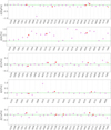 |
Fig. 4 Differences in median abundances of [Mg/Fe], [Al/Fe], [Si/Fe], [K/Fe], and [Ca/Fe] between 1P and 2P stars (violet) and 1P and anomalous stars (red). Symbols and lines follow the same conventions as in Figure 3. The orange starred symbol refers to the host galaxy remnant of NGC 7089. |
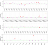 |
Fig. 5 Differences in median abundances of [Ti/Fe], [Fe/H], [Ni/Fe], and [Ba/Fe] between 1P and 2P stars (violet) and 1P and anomalous stars (red). Symbols and lines follow the same conventions as in Figure 3. |
4 Spread of elements among globular clusters
As shown in Figure 6, the difference in 1P and 2P abundances for a given element can vary significantly from one cluster to another. For instance, Δ[Al/Fe] ranges from almost zero in NGC 6838 to nearly 1 dex in NGC 6254, while oxygen depletion is negligible in NGC 4590 but around 0.8 dex in NGC 6402. This indicates that the abundance ratios can exhibit vastly different spreads across various GCs. In this section, we explore this variability, with particular focus on the elements that show clear patterns of distinct average abundances, specifically carbon, nitrogen, oxygen, sodium, magnesium, and aluminum.
However, ΔX is not the most effective metric in this context, as it may underestimate the total abundance spread. This is particularly true in cases where 2P stars span a wide range of light-element abundances, as observed in clusters such as NGC 2808, NGC 6218, and NGC 6752 (e.g., Carretta et al. 2007a; Johnson & Pilachowski 2012; Carlos et al. 2023), or display the most extended ChMs (Milone et al. 2017). To address this, we introduce a more appropriate measure, the total width WX, where X represents any given abundance ratio. WX was calculated as the difference between the 90th and 10th percentiles of the elemental distribution of all the stars in the photometric catalogs with spectroscopically measured chemical abundances, including those without ChM tagging (therefore disregarding their association with a specific population). This approach allowed us to use a larger sample of stars in each cluster compared to the analysis in Section 3. Notably, this allowed us to also include NGC 5986, NGC 6388, and NGC 6934, which did not pass the strict selection criteria applied in Section 3. We accounted for observational errors by subtracting in quadrature the contribution of the average uncertainty, measured by applying our procedure to a simulated distribution of points scattered by the average uncertainty provided by the source datasets. For abundances with multiple determinations, we calculated the final WX by averaging the individual widths, weighted by their errors. As in Section 3, to calculate W[C/Fe] and W[N/Fe] we only considered RGB stars fainter than the bump. Measures that were possible only with stars above the bump are indicated, for completeness, in gray, and were not included in the analysis performed in the rest of this section.
In Figure 7, we present the width distributions relative to cluster mass and metallicity7. Lithium and barium are excluded, as their distributions will be addressed separately in Sections 6 and 7, respectively. For each plot, we provide the Spearman rank correlation coefficient along with the p-value (in parentheses), which represents the probability that two intrinsically independent variables could produce the observed distribution. The spreads of carbon, nitrogen, oxygen, and magnesium show Spearman coefficients and p-values consistent with a correlation with cluster mass. Additionally, silicon also shows a mild correlation with log(M/M⊙). Our results are in qualitative agreement with the analysis recently published by Lee et al. (2025), who also detected that the dispersion in [C/Fe] and [N/Fe] abundances increases with cluster mass. Conversely, our dataset does not suggest any correlation between the nitrogen spread and [Fe/H], in contrast to the findings of Lee and collaborators.
The two most massive GCs, NGC 5139 and NGC 6715, are both Type II clusters with significant iron enhancement, clearly reflected in their large W[Fe/H] values. Moreover, iron content plays a significant role, as the overall [Fe/H] is found to anticorrelate with W[Al/Fe] and W[K/Fe] and exhibits a mild anticorrelation with W[Ni/Fe]. Potassium represents an intriguing case: the W[K/Fe] distribution remains almost flat for [Fe/H]> −1.5 dex but increases sharply at lower metallicities. This distinct behavior may be due to the activation of the Ar–K chain, which could lead to K-enhanced 2P stars, as suggested by previous studies (e.g., Mucciarelli et al. 2015; Mészáros et al. 2020). However, in Figure 4, we clearly observed this phenomenon only in NGC 2419 and, to a lesser extent, in NGC 3201, NGC 2808, and NGC 6752, likely due to the small sample size of stars with both [K/Fe] measurements and ChM tagging in other GCs, which limits statistical significance. NGC 7078, one of the most metal-poor clusters in the sample, stands out as an exception with a very small W[K/Fe].
For some abundance ratios, upper limits were reported in certain datasets beyond the observational measurements. Specifically, [O/Fe] obtained through the [O I] forbidden lines at 6300.3 and 6363.8 Å frequently present such cases. As noted in Section 2, we did not include upper limits in our width estimates. While this exclusion could, in principle, lead to an underestimation of the elemental spread – particularly if some GCs host stars with extremely low oxygen abundances – we evaluated this potential bias by remeasuring elemental spread with upper limits included. Our findings indicate that, excluding the upper limits, the differences in the spreads are negligible in most cases, but can sometimes reach up to ~0.10 mag. Overall, we consider this bias negligible and comparable to the typical observational errors (0.03–0.20 mag for W[O/Fe]). Nevertheless, although we verified that all stellar populations, including the most extreme ones in the ChMs, were sampled with O-abundance measurements, we cannot exclude the presence of stars with very low (undetectable) O in clusters like NGC 2808. In such cases our measured spreads would be overestimated.
In Figure 8, we focus on the elements that, according to our findings in Section 3, display evident and widespread variation patterns among different populations: carbon, nitrogen, oxygen, sodium, magnesium, and aluminum. We separately analyze the total spread of these elements against cluster mass and metallicity for the two reaction chains responsible for the observed multiple-population patterns: CNONa (WC,N,O,Na, panels (a1) and (a2)) and MgAl (WMg,Al, panels (b1) and (b2)). The CNONa spread shows a clear correlation with cluster mass, whereas the MgAl spread demonstrates a weaker correlation. WMg,Al displays a statistically significant anticorrelation with [Fe/H], strongly supported by the metallicity dependence observed in the Δ[Al/Fe] vs. Δ[Mg/Fe] diagram in Figure 6. To account for metallicity effects on the WMg,Al vs. mass relation, we applied a method similar to that of Milone et al. (2017). Specifically, we selected a narrow mass range where GCs exhibit significant variation in WMg,Al values. Within this range, the influence of mass on WMg,Al is minimal, suggesting that the variability is primarily driven by metallicity differences. We chose the range 5.5 < log(M/M⊙) < 5.9, where WMg,Al spans values from approximately 0.3 mag to 1.7 mag. As expected, the selected GCs (highlighted in yellow in panels (b1) and (b2)) cover a wide [Fe/H] range of about 1 dex. To remove the metallicity effect, we fit these clusters in the WMg,Al vs. [Fe/H] plane with a straight line. The difference between WMg,Al and the best-fit line, denoted as ΔWMg,Al, was then calculated. As shown in panel (b3), this adjustment strengthens the correlation between WMg,Al and cluster mass. Finally, we calculated the overall spread of the six light elements, WC,N,O,Na,Mg,Al, by summing the CNONa spread and the metallicity-corrected MgAl spread. As illustrated in panel (c1), this combined quantity exhibits a strong correlation with GC mass.
Helium is another element involved in the multiple population phenomenon. Milone et al. (2018) calculated its total spread (δYmax) based on the ChM positions of 1P and 2P stars, showing that more massive GCs tend to have larger helium variations. In panel (c2), we establish, for the first time, a connection between the spread of light elements derived from spectroscopy with the δYmax for a large sample of GCs. We found a strong correlation between these two quantities, demonstrating the link between helium and other light elements in the multiple populations phenomenon.
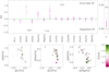 |
Fig. 6 Upper panels: difference between the median of the 2P and 1P abundance of each analyzed element. Positive and negative values (above and below the green line), represent enrichment and depletion of 2P stars, respectively. The right panel displays the 2P–1P helium difference (in mass fraction) from Milone et al. (2018). Lower panels: diagrams of Δ[N/Fe] vs. Δ[C/Fe] (left), Δ[Na/Fe] vs. Δ[O/Fe] (middle), and Δ[Al/Fe] vs. Δ[Mg/Fe] (right). Each point is color coded according to their [Fe/H], following the scheme represented in the color bar. Smaller dots indicate Δ[C/Fe] and Δ[N/Fe] based on RGB stars above the bump. |
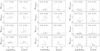 |
Fig. 7 Total spread of [C/Fe], [N/Fe], [O/Fe], [Na/Fe], [Mg/Fe], [Al/Fe], [Si/Fe], [K/Fe], [Ca/Fe], [Ti/Fe], [Fe/H], and [Ni/Fe] with respect to the clusters’ mass and average metallicity. In each plot, we report the Spearman correlation coefficient, with its significance (p-value) in round parentheses. Gray points are relative to W[C/Fe] and W[C/Fe] measurements based on stars below the RGB bump. |
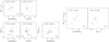 |
Fig. 8 Panels (a1) and (a2): WC,N,O,Na vs. log(M/M⊙) and [Fe/H], respectively. Panels (b1) and (b2): same as panels (a1) and (a2) but for WMg,Al. GCs within the 5.5 < log(M/M⊙) < 5.9 mass interval used to remove the metallicity dependence (see text for details) are encircled in yellow. Panel (b3): resulting width after removing [Fe/H] dependence (ΔWMg,Al) vs. mass. Panels (c1) and (c2): total width of light elements involved in the multiple population phenomenon WC,N,O,Na,Mg,Al vs. mass and maximum helium spread measured by Milone et al. (2018), respectively. The Spearman correlation coefficient and its p-value are reported in each plot as in Figure 7. |
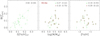 |
Fig. 9 Left panel: 1P stars [Fe/H] spread from spectroscopy |
![$\[\left(W_{[\mathrm{Fe} / \mathrm{H}]}^{\mathrm{IP}}\right)\]$](/articles/aa/full_html/2025/05/aa53024-24/aa53024-24-eq2.png)
![$\[W_{[\mathrm{Fe} / \mathrm{H}]}^{\mathrm{IP}}\]$](/articles/aa/full_html/2025/05/aa53024-24/aa53024-24-eq3.png)
5 Metallicity variations among first-population stars
One of the most intriguing recent discoveries about GCs is the presence of chemical inhomogeneities among 1P stars. Their distribution along the x-axis of the ChM is significantly broader than what is expected by observational errors only (e.g., Milone et al. 2017; Dondoglio et al. 2021; Jang et al. 2022). Moreover, metallicity inhomogeneities were also detected in NGC 0104, NGC 5272, NGC 6341, and NGC 6656 (Lee & Sneden 2021; Lee 2022, 2023, 2024) through the JWL indices derived from ground-based photometry (e.g., Lee 2017). Spectroscopic observations revealed that the most likely driver of this feature is the presence of star-to-star iron variation among them (Marino et al. 2019b; Legnardi et al. 2022; Carlos et al. 2023; Marino et al. 2023). Legnardi et al. (2022), by assuming that the ChM spread is due to iron variations only, predicted the necessary 1P [Fe/H] spread, δ[Fe/H]1P, to justify their ChM dispersion.
Our dataset allowed us to investigate the presence of iron variations among 1P stars and its relation with the elongation along the x-axis of the ChM. To achieve this, we calculated the spread of [Fe/H], ![$\[W_{[\mathrm{Fe} / \mathrm{H}]}^{1 \mathrm{P}}\]$](/articles/aa/full_html/2025/05/aa53024-24/aa53024-24-eq4.png) , among 1P stars by following the same method described in Section 4 to estimate the elemental spreads. We considered only clusters with spectroscopic datasets containing at least ten 1P stars except for NGC 5024. Despite fulfilling this criterion, NGC 5024 has iron measurements only for stars spanning a ΔF275W,F814W much smaller than the spread of 1P stars over the ChM, which may possibly lead to an underestimation of its [Fe/H] spread.
, among 1P stars by following the same method described in Section 4 to estimate the elemental spreads. We considered only clusters with spectroscopic datasets containing at least ten 1P stars except for NGC 5024. Despite fulfilling this criterion, NGC 5024 has iron measurements only for stars spanning a ΔF275W,F814W much smaller than the spread of 1P stars over the ChM, which may possibly lead to an underestimation of its [Fe/H] spread.
The left panel of Figure 9 represents ![$\[W_{[\text{Fe/H}]}^{\mathrm{IP}}\]$](/articles/aa/full_html/2025/05/aa53024-24/aa53024-24-eq5.png) vs. δ[Fe/H]1P, demonstrating that our direct measurements are in agreement with the prediction by Legnardi et al. (2022), as they are distributed around the one-to-one relation indicated by the gray line. Moreover, the two quantities correlate with each other, as supported by the Spearman’s coefficient of 0.60 and a p-value <0.01. Our measurement of metallicity spread spans an interval from ~0.00 to 0.25 dex, with NGC 5272 (M3) exhibiting the largest value. We found that only three GCs are consistent within 1-σ with a negligible spread in [Fe/H] (NGC 0288, NGC 7089, and NGC 7099), while for the other 19 we confirm the presence of non-negligible iron inhomogeneities. The central and right panels represent
vs. δ[Fe/H]1P, demonstrating that our direct measurements are in agreement with the prediction by Legnardi et al. (2022), as they are distributed around the one-to-one relation indicated by the gray line. Moreover, the two quantities correlate with each other, as supported by the Spearman’s coefficient of 0.60 and a p-value <0.01. Our measurement of metallicity spread spans an interval from ~0.00 to 0.25 dex, with NGC 5272 (M3) exhibiting the largest value. We found that only three GCs are consistent within 1-σ with a negligible spread in [Fe/H] (NGC 0288, NGC 7089, and NGC 7099), while for the other 19 we confirm the presence of non-negligible iron inhomogeneities. The central and right panels represent ![$\[W_{[\mathrm{Fe} / \mathrm{H}]}^{\mathrm{P}}\]$](/articles/aa/full_html/2025/05/aa53024-24/aa53024-24-eq6.png) vs. the logarithm of the cluster mass and average metallicity, respectively. The criterion provided by the Spearman’s coefficient does not suggest that
vs. the logarithm of the cluster mass and average metallicity, respectively. The criterion provided by the Spearman’s coefficient does not suggest that ![$\[W_{[\mathrm{Fe} / \mathrm{H}]}^{\mathrm{P}}\]$](/articles/aa/full_html/2025/05/aa53024-24/aa53024-24-eq7.png) correlates with either of the two quantities. However, we point out that the GCs with the largest spread are mostly present at log(M/M⊙) > 5.5. Additionally, when considering the M3-like GCs (classified as in Milone et al. 2014; Tailo et al. 2020 and encircled in brown),
correlates with either of the two quantities. However, we point out that the GCs with the largest spread are mostly present at log(M/M⊙) > 5.5. Additionally, when considering the M3-like GCs (classified as in Milone et al. 2014; Tailo et al. 2020 and encircled in brown), ![$\[W_{[\mathrm{Fe} / \mathrm{H}]}^{\mathrm{P}}\]$](/articles/aa/full_html/2025/05/aa53024-24/aa53024-24-eq8.png) displays a mild anticorrelation with [Fe/H]. Overall, our results suggest that both cluster mass and average metallicity are in some way linked to the phenomenon (especially among M3-like GCs), qualitatively in agreement with the prediction by Legnardi et al. (2022).
displays a mild anticorrelation with [Fe/H]. Overall, our results suggest that both cluster mass and average metallicity are in some way linked to the phenomenon (especially among M3-like GCs), qualitatively in agreement with the prediction by Legnardi et al. (2022).
We next investigated the relation between the [Fe/H] distribution of 1P stars and their extension along the x-axis of the ChMs. A correlation between the two quantities has been identified in NGC 0104, NGC 3201, NGC 6254 (Marino et al. 2019a,b, 2023) by comparing spectroscopic abundances to HST-based ChMs. Here, we extend this analysis to a larger sample of GCs, also considering the extension of 1P stars along the ground-based ChM. For the latter, we do not use the ChM built by Jang et al. (2022), but instead employ a ChM that uses the U − I color rather than the B − I on its x-axis. The former filter combination ensures a wider color baseline than the latter, and thus is more sensitive to possible metallicity variations. To maximize the sample of stars with [Fe/H] measurement and ChM tagging, we combined iron measurements from various studies for each cluster. To account for potential systematic differences between different studies, we calculated the average [Fe/H] difference among stars common to the dataset with the largest amount of stars and every other dataset and then shifted each dataset by this quantity. Typically, the average shift between different datasets was in the ~0.00–0.15 dex interval. For stars present in more than one dataset, we considered the combined [Fe/H] derived by averaging the different measurements (after correcting for eventual systematics).
Figure 10 represents our results for eight GCs in our sample, namely NGC 0104, NGC 1261, NGC 3201, NGC 4833, NGC 5272, NGC 5904, NGC 6254, and NGC 6715. We show the [Fe/H] vs. ΔF275W,F814W and ΔU,I for each cluster, when available. Comparison with HST and ground-based ChMs are presented in the odd and even columns, respectively. NGC 0104, NGC 1261, and NGC 6254 exhibit an increase in [Fe/H] toward redder colors in both ChMs, with Spearman coefficients consistent with mild-to-strong correlations. NGC 3201, the other GC with a significant number of 1P stars with iron abundances in both ChMs, shares this behavior only in the innermost region covered by HST observations while no significant trend is observed with ΔU,I. NGC 4833, NGC 5272, and NGC 5904 have spectroscopic information only for the stars in the ground-based ChM, whereas for NGC 6715, this analysis is feasible only using HST photometry. These four GCs also show that their ΔF275W,F814W and ΔU,I 1P extensions are linked to their iron abundance.
Moreover, Marino et al. (2023) found that in NGC 0104 the absolute abundances of other elements analyzed follow the same trend of [Fe/H]. In particular, they show that the average abundance of α elements increases with ΔF275W,F814W among 1P stars (see their Figure 6). Motivated by this result, we investigated the same quantity in six of the GCs shown in Figure 10, which have available Si, Ca, and Ti estimates that we use as proxies for the α-element abundance. Results are illustrated in Figure 11, where the average absolute α element abundance, logϵ(α), is represented8. NGC 0104 is the only GC with measurements of 1P stars in both HST and ground-based ChM, for which we exploited the Marino et al. (2023) and APOGEE datasets, respectively. The APOGEE dataset also allowed us to measure this quantity in NGC 3201, NGC 5272, NGC 5904, and NGC 6254, while for NGC 1261 we used the GES abundances. In NGC 0104, our data are consistent with a correlation between the α elements and both the ΔF275W,F814W and the ΔU,I. NGC 5272 and NGC 6254 also display a correlation with the x-axis of the ChM, while for NGC 1261 and NGC 5904 (the other two clusters with a sign of [Fe/H] correlation detected in Figure 10), no clear correlation is suggested by the Spearman’s coefficient. Finally, NGC 3201 does not display an evident trend between these two quantities, in agreement with the lack of iron correlation with ΔU,I.
The results presented in this section indicate that iron variations among 1P stars are widespread across GCs. These overall metallicity differences are the principal cause of the color spread observed in the ChM.
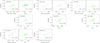 |
Fig. 10 [Fe/H] abundance for 1P stars vs. ΔF275W,F814W and/or ΔU,I (depending on the availability of iron spectroscopic measurements) of NGC 0104, NGC 1261, NGC 3201, NGC 4833, NGC 5272, NGC 5904, NGC 6254, and NGC 6715. Grey lines indicate the best-fit straight line. Correlation coefficients are reported in each plot. Comparison of iron abundances with HST and ground-based x-axis of the ChMs are aligned along the even and odd columns on the image, respectively. |
6 Lithium among multiple populations
Lithium plays a critical role in constraining the origins of multiple stellar populations, particularly in identifying the nature of the polluters responsible for the processed material from which 2P stars formed. As noted by D’Antona et al. (2019), polluters that generate gas processed through hydrogen burning in their convective envelopes are thought to completely destroy lithium. As such, any lithium observed in 2P stars must result from dilution between pristine gas and the lithium-free material that formed these stars. In contrast, if intermediate-mass asymptotic giant branch (AGB) stars are the source of the processed gas, they could account for lithium in 2P stars without dilution, as they produce it through the Cameron-Fowler mechanism (Cameron & Fowler 1971).
As discussed in Section 3, 2P stars generally show slightly lower lithium levels than 1P stars. Here, we focus on 2P stars with more extreme chemical compositions (2Pext), which are believed to have undergone minimal, if any, dilution (e.g., D’Antona et al. 2016). For this analysis, we used eight GCs from the first row of Figure 3, as well as ωCen, which has only two 1P stars with A(Li) measurement and therefore does not meet the criteria for detailed analysis discussed in Section 3.
The first step was to identify a sample of 2Pext stars, which typically display the highest y-axis coordinates in the ChM. Numerous studies have shown that stars positioned higher on the y-axis of the ChM have chemical compositions that deviate more from 1P stars (e.g., Marino et al. 2019a; Carlos et al. 2023; Carretta & Bragaglia 2024). Figure 12 illustrates the relationship between the y-axis position in the ChM and A(Li) for each GC. We present both the HST and ground-based ChMs, as well as the two HST datasets for ωCen, for all GCs except NGC 1904 (which only has ground-based data) and NGC 6121 for the Mucciarelli et al. (2011) catalog (which lacks lithium measurements in the HST-based diagram). We defined 2Pext stars as those above the 70th percentile of the y-axis distribution, indicated by the blue dashed horizontal line. This calculation included upper limits (excluded in Section 3), represented by arrows colored according to their population. For NGC 2808 and NGC 6121, where lithium measurements are available from multiple datasets, both are shown separately in the figure. For each GC, we display the median A(Li) values for 1P and 2Pext stars using green and blue starred symbols, respectively, with bands around the points representing uncertainties. 2Pext stars exhibit significantly lower A(Li) than 1P stars in all GCs except NGC 6121, NGC 6809, and NGC 6838. In the cases of ωCen and NGC 6656, we applied a similar procedure to compare 1P stars with anomalous stars. Here, the 70th percentile line is shown in red, and the average A(Li) for extreme anomalous stars (Aext) is represented by a red starred symbol. In both clusters, anomalous stars are more lithium-depleted than the 2Pext stars.
As in Section 3.2, we defined Δ2PextA(Li) or ΔAextA(Li) as the difference between the median A(Li) values of 2Pext (or Aext) and 1P stars. For NGC 2808 and NGC 6121, we averaged the results from the separate datasets to obtain the final Δ2PextA(Li). Figure 13 shows the trend of Δ2PextA(Li) and ΔAextA(Li), represented by open black points and red crosses, respectively, with GC mass and the δYmax measured by Milone et al. 2018, in the left and right panels.
Overall, Δ2PextA(Li) is wider (i.e., more negative) both at larger GC mass and helium spread. This trend may seem qualitatively consistent with the dilution hypothesis, as less massive and less He-enriched GCs are expected to host more diluted 2P stars, which would be more lithium-rich. However, we highlight two key points: (i) in clusters where Δ2PextA(Li) is close to zero, 2P stars would almost entirely consist of pristine material. This is difficult to reconcile with the large sodium and nitrogen differences observed in these same clusters. (ii) Even in GCs with the largest ![$\[\Delta_{\mathrm{A}(\mathrm{Li})}^{2 \text {Pext}}\]$](/articles/aa/full_html/2025/05/aa53024-24/aa53024-24-eq9.png) , their 2Pext stars exhibit a wide lithium spread partially overlapping the 1P A(Li) distribution. NGC 2808, the most helium-enriched cluster in our sample, is a notable example of this, indicating that even the least diluted 2P stars formed from gas with a non-negligible amount of lithium.
, their 2Pext stars exhibit a wide lithium spread partially overlapping the 1P A(Li) distribution. NGC 2808, the most helium-enriched cluster in our sample, is a notable example of this, indicating that even the least diluted 2P stars formed from gas with a non-negligible amount of lithium.
These observational constraints qualitatively show that dilution alone cannot justify the amount of lithium observed in 2P stars, but an additional production mechanism in the polluter is necessary. AGB stars have been traditionally seen as the most likely candidates. However, it remains to be explored whether other candidates (e.g., massive interacting binaries) may also produce lithium at some point in their evolution.
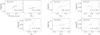 |
Fig. 11 Same as Figure 10 but for logϵ(α) vs. ΔF275W,F814W (only for NGC 0104) and ΔU,I for NGC 0104, NGC 1261, NGC 3201, NGC 5272, NGC 5904, and NGC 6254. |
7 Type II globular clusters
In this section, we examine the chemical composition of anomalous stars in detail, investigating their internal abundance variations and their distinctions from canonical stars (e.g., the bulk of 1P and 2P). We used data from the dataset with the highest incidence of anomalous stars (i.e., the ratio of anomalous stars to the total spectroscopically analyzed stars) rather than averaging across multiple datasets available in the literature.
Figure 14 presents the [C/Fe] vs. [N/Fe], [O/Fe] vs. [Na/Fe], and [Mg/Fe] vs. [Al/Fe] diagrams in the left, central, and right rows, respectively, for anomalous stars (represented by red filled dots). For comparison, 1P and 2P stars are also displayed. Each plot specifies the dataset considered.
[C/Fe] and [N/Fe] measurements for stars brighter than the RGB bump are marked with crosses. For ωCen, we included two separate datasets (APOGEE and Marino et al. 2012), as they capture different segments of the complex anomalous star population: while most APOGEE measurements involve stars near the 1P and 2P in the ChM, stars from Marino et al. (2012) populate regions with higher average ΔF275W,F814W values. Although the Marino et al. (2012) measurements cover stars above the RGB bump, the stars shown in the figure span a relatively small ~2 mag range, minimizing magnitude effects. In the [O/Fe] vs. [Na/Fe] and [Mg/Fe] vs. [Al/Fe] plots, employing two datasets is unnecessary, as the available measurements sufficiently span the entire anomalous population in the ChM. Notably, in four GCs (NGC 1851, ωCen, NGC 6656, and NGC 6715), anomalous stars exhibit chemical inhomogeneities similar to 1P–2P patterns but with more chemically extreme average values. In NGC 6656, anomalous stars display higher average carbon than the canonical population, consistent with Marino et al. (2011). A similar trend was observed in ωCen using the Marino et al. (2012) dataset, where some anomalous stars exhibit higher [C/Fe] values compared to the rest. In the remaining six GCs, limited sample sizes hindered the identification of clear trends. However, anomalous stars in NGC 0362, NGC 1261, and NGC 5286 exhibit light-element abundances comparable to or more extreme than 2P stars, aligning with previous spectroscopic results (Carretta et al. 2013b; Marino et al. 2015, 2021). Conversely, anomalous stars in NGC 6934 are depleted in Al and Na relative to 2P stars, although one star shows Na enhancement. For NGC 7089, we included the metal-rich population identified by Yong et al. (2014), likely associated with a remnant host galaxy (see Milone et al. 2015), which exhibits Mg and Al abundances similar to those of 1P stars. Its sole anomalous star overlaps with the 2P region. In NGC 6388, the anomalous population showed no significant differences from canonical stars in the [Na/Fe] vs. [O/Fe] and [Mg/Fe] vs. [Al/Fe] diagrams.
Anomalous stars are linked with enrichment in iron, s-process elements, and total C+N+O compared to the rest of the clusters’ stars (e.g., Yong & Grundahl 2008; Marino et al. 2009; Carretta et al. 2011; Marino et al. 2015; McKenzie et al. 2022; Dondoglio et al. 2023). Accordingly, we explored their [Fe/H], [Ba/Fe] (as an s-process element proxy), and [C+N+O/Fe] distributions. Figure 15 illustrates the [Ba/Fe] vs. [Fe/H] diagram for eight Type II GCs. In NGC 1851 and NGC 5286, anomalous stars cluster around higher average barium levels and, for NGC 5286, higher iron levels, while still overlapping somewhat with canonical stars. These findings are consistent with spectroscopic investigations Carretta et al. (2011); Marino et al. (2015). In ωCen, this effect is more pronounced, with anomalous stars showing a broad distribution (spanning over 1 dex) in both elements, far exceeding observational error. Iron-rich stars also tend to show greater barium abundances. In NGC 0362, NGC 1261, NGC 6934, and NGC 7089, the limited sample size resulted in low statistical significance. In NGC 0362, anomalous stars span a similar [Fe/H] range as canonical stars but show slightly higher barium levels, consistent with the enhancement identified by Carretta et al. (2013a). In NGC 1261 and NGC 6934, anomalous stars are more iron-rich than canonical stars but have comparable [Ba/Fe], aligning with Marino et al. (2021). For NGC 7089, anomalous stars exhibit similar barium and iron levels, consistent with Yong et al. (2014), who identified a group of Ba- and Fe-rich stars. Discrepancies are likely due to the small sample size used in our ChM tagging. The single star associated with the remnant of NGC 7089’s host galaxy, as estimated by Yong et al. (2014), is approximately 0.5 dex [Fe/H]-richer than the other stellar populations.
Figure 16 displays the kernel density distributions of [C+N+O/Fe] for canonical (black) and anomalous (red) stars in NGC 1851, ωCen, and NGC 6656. These distributions were derived using APOGEE data, except for ωCen, where abundances from Marino et al. (2012) were also used. Dash-dotted lines indicate distributions for stars above the RGB bump. In NGC 1851, the distributions partially overlap, but anomalous stars generally show higher [C+N+O/Fe] values, suggesting CNO enhancement (as derived by Yong et al. 2015; Dondoglio et al. 2023). APOGEE data revealed significant variability among anomalous populations within this massive GC, with some stars showing CNO enhancement relative to canonical stars and others displaying similar levels. Anomalous stars in the dataset from Marino et al. (2012) show a similar spread, but are centered at higher values, highlighting greater enhancement. This difference likely reflects the inclusion of anomalous stars farther from the 1P and 2P bulk along the ChM in the dataset of Marino and colleagues, which tend to exhibit wider chemical inhomogeneities. In NGC 6656, anomalous stars are clearly CNO-enhanced, with their [C+N+O/Fe] distribution peaking about 1 dex higher than that of canonical stars.
Next, in Figure 17 we assessed the relationship between iron and barium enrichment in anomalous stars and the mass of their host cluster. Following the approach in Section 4, we measured the spreads W[Fe/H] and W[Ba/Fe]. Results are shown as black dots, while clusters with fewer than ten stars (excluded following Section 4 guidelines) are in cyan. The iron spread tends to increase in more massive clusters, with the highest values observed in ωCen. Among lower-mass clusters (log(M/M⊙) < 5.6), three out of the four clusters have minimal iron spread. Notable exceptions include NGC 6934, which exhibits significant W[Fe/H] despite being the least massive, and NGC 6388, the third most massive Type II cluster, which shows negligible iron spread (see also Marino et al. 2021; Carretta & Bragaglia 2022). Similarly, W[Ba/Fe] correlates with mass, although NGC 6388 remains an outlier with no measurable barium spread.
Our analysis demonstrates that, relative to canonical stars, anomalous stars are generally enhanced in iron, barium (and likely other s-process elements), and total C+N+O, though with a few exceptions. This indicates that these stars formed from gas polluted by products of different sources compared to those involved in the formation of 2P stars, such as core-collapse supernovae of massive stars and intermediate-mass AGB stars (see the discussion in Dondoglio et al. 2023, and reference therein).
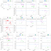 |
Fig. 12 The y-axis of the ChM vs. A(Li). Measurements and upper limit (arrows) are color coded according to their population. For each GC, the bottom panel refers to stars in the innermost areas covered by HST observations, while the upper ChM regards stars outside the central field (covered by ground-based photometry in all GCs except ωCen). Horizontal blue and red dashed lines indicate the 70-th percentile level of the 1P+2P and 1P+anomalous star distributions, respectively. Above the ChMs, starred green and blue symbols denote the median 1P and 2Pext A(Li), shifted arbitrarily on the y-axis for illustration purposes. |
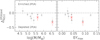 |
Fig. 13 Difference between lithium abundances for the most extreme 2P stars and the 1P stars (open black dots) vs. the cluster mass and maximum helium spread (right and left panels, respectively). Red crosses indicate the same quantity but measured for anomalous stars (see text for details). |
8 Conclusions
In this work, we identified 1P and 2P stars in 38 Galactic GCs using ChMs derived by Milone et al. (2017) and Jang et al. (2022) from HST and ground-based photometry, along with newly introduced ChMs for ωCen, NGC 5286, and NGC 6656. We also scanned ~20 years of spectroscopic analyses to infer chemical abundances for photometrically tagged stars. This sample includes ~3200 stars across 38 GCs, focusing on the abundances of 14 elements (Li, C, N, O, Na, Mg, Al, Si, K, Ca, Ti, Fe, Ni, and Ba).
The observed carbon and oxygen depletion, alongside the enrichment in nitrogen and sodium among 2P stars is consistent with contributions from material that underwent CNO-cycling and p-capture processes at high temperatures (such as the Ne–Na cycle) during the formation of this population. Magnesium is modestly depleted in 2P stars (except for NGC 2419), while aluminum displays the largest observed enhancements. The most metal-rich GCs in our sample tend to display small-to-nil [Mg/Fe] and [Al/Fe] variations, while the differences between 1P and 2P stars increase with decreasing metallicity. These findings strongly suggest that the material from which 2P stars formed also underwent the Mg–Al cycle, which requires temperatures above ~70 MK and hence operates more effectively at lower metallicities, where it depletes magnesium and produces aluminum. Similarly, significant potassium spread occurs below [Fe/H] ~−1.5, increasing further at lower metallicities (Figure 7), likely due to activation of the Ar–K chain. Two GCs emerged as notable outliers in our analysis. In NGC 6402, 2P stars show ~0.9 dex [O/Fe] depletion relative to 1P stars, which is a much larger variation than in any other GC in our sample. The peculiarity of NGC 6402 lies in the fact that, although the [O/Fe] depletion among its most extreme 2P stars is roughly similar to that observed in NGC 2808, all 2P stars in NGC 6402 have very low oxygen abundances. In contrast, NGC 2808 hosts different 2P populations with intermediate oxygen composition. Although other light elements (Na, Mg, and Al) exhibit some of the largest differences between 1P and 2P stars, they align more closely with the general GC trend. D’Antona et al. (2022) proposed that this cluster may be Type II, potentially explaining its unusual behavior, although the limited number of photometrically tagged stars with abundance measurements complicates drawing firm conclusions. In NGC 2419, 2P stars show extreme magnesium depletion and potassium enhancement. Mucciarelli et al. (2011) suggest that the cluster’s large distance from the Galactic center, and its limited interaction with the Milky Way, could facilitate retention of processed material. Ventura et al. (2012) further propose that extreme Mg and K variations are more likely at low metallicities. However, additional measurements, particularly for O, Na, and Al, which are currently available only for a few stars without ChM tagging (Cohen et al. 2011; Cohen & Kirby 2012), are needed to confirm this model. These factors, combined with NGC 2419’s large mass – typically associated with greater light-element inhomogeneity – may explain its unique chemical profile.
The 1P–2P chemical patterns observed in this work align well with previous studies on multiple populations, based on both photometry and spectroscopy (e.g., Carretta et al. 2009; Pancino et al. 2017; Milone et al. 2018; Marino et al. 2019a; Mészáros et al. 2020). Our sample constitutes the largest census to date of chemical differences among multiple populations in GCs, in terms of clusters, stars, and elemental diversity.
We find that the mass of the host cluster plays an important role in the phenomenon of multiple populations. Indeed, the combined spread of the six light elements that show widespread 1P–2P differences correlates with this quantity, a trend that becomes clearer when metallicity dependence is removed. Furthermore, the spread in these elements is strongly linked to helium variation, as GCs with greater He enhancement also display broader spreads in elements linked to multiple populations. These findings provide spectroscopic evidence supporting earlier photometric results (e.g., Milone et al. 2017, 2018; Lagioia et al. 2025).
For 22 GCs in our sample, we measured the [Fe/H] spread among 1P stars, ![$\[W_{[\mathrm{Fe} / \mathrm{H}]}^{\mathrm{P}}\]$](/articles/aa/full_html/2025/05/aa53024-24/aa53024-24-eq10.png) , finding that only three clusters are consistent with negligible spread at a 1-σ-level, suggesting a constant [Fe/H]. This study represents the largest sample analysis of this phenomenon based on direct [Fe/H] measurements obtained from spectroscopy. Our results generally agree with photometric predictions by Legnardi et al. (2022), supporting the role of GC mass and metallicity in influencing this behavior. In eight GCs, we observed a correlation between iron abundance in 1P stars and their position on the ChM x-axis, where redder stars tend to be more metal-rich. In three clusters, a similar correlation with the abundance of α-elements supports the idea that chemical differences among 1P stars reflect broader metallicity differences beyond iron alone (see Marino et al. 2023). Notably, this is the first time these patterns have been detected in ChMs constructed with UBVI filters.
, finding that only three clusters are consistent with negligible spread at a 1-σ-level, suggesting a constant [Fe/H]. This study represents the largest sample analysis of this phenomenon based on direct [Fe/H] measurements obtained from spectroscopy. Our results generally agree with photometric predictions by Legnardi et al. (2022), supporting the role of GC mass and metallicity in influencing this behavior. In eight GCs, we observed a correlation between iron abundance in 1P stars and their position on the ChM x-axis, where redder stars tend to be more metal-rich. In three clusters, a similar correlation with the abundance of α-elements supports the idea that chemical differences among 1P stars reflect broader metallicity differences beyond iron alone (see Marino et al. 2023). Notably, this is the first time these patterns have been detected in ChMs constructed with UBVI filters.
We next investigated lithium variation in nine GCs, focusing on the composition of their most chemically extreme 2P stars, 2Pext. Even among these stars, lithium depletion reaches a maximum of ~0.3 dex in the clusters with the largest mass and He-richer 2Pext. Conversely, it is consistent with zero in the least massive cluster, which typically exhibits the smallest helium variations. These results suggest that lithium depletion is not a common feature of all clusters hosting multiple populations but rather is experienced only by the most chemically extreme 2P. These stars typically reside in the most massive GCs with large helium variations. Even within this category, some of the 2Pext stars exhibit a lithium abundance that overlaps the 1P distribution. Our extended investigation of literature A(Li) abundances, combined with the population tagging provided by the ChM, provides robust confirmation of the conclusions of previous studies (e. g., D’Orazi et al. 2014, 2015; Aguilera-Gómez et al. 2022; Schiappacasse-Ulloa et al. 2022). Our findings support a scenario in which the lithium present among 2P stars would not entirely originate from dilution with pristine material, necessitating a process that produces this element in the polluted gas.
AGB stars constitute an appealing candidate, as they can provide extra lithium through the Cameron & Fowler (1971) process (see the discussion in D’Antona et al. 2019), but it remains to be seen to what extent other polluters, for example massive interacting binaries, could also produce some lithium.
Finally, we analyzed the chemical composition of anomalous stars in ten Type II GCs, finding that light-element inhomogeneities are common in several clusters (e.g., NGC 1851, ωCen, NGC 6656, and NGC 6715), though not universally. In most clusters, anomalous stars have chemical compositions closer to 2P than 1P stars, with the possible exception of NGC 6934. Anomalous stars typically show larger barium (a proxy for s-process elements) and iron abundances, though these enhancements do not always co-occur. Some clusters display enrichment in only one of these elements, with NGC 6388 showing neither. Remarkably, ωCen exhibits pronounced enhancement in both, with its most Fe-rich anomalous stars also being the most Ba-rich.
In NGC 1851, ωCen, and NGC 6656, we combined photometric tagging with carbon, nitrogen, and oxygen abundances, finding that anomalous stars (in the case of ωCen only a fraction of the stars) generally show higher [C+N+O/Fe] than canonical stars. The presence of iron, barium (and likely other s-process elements), and C+N+O enhancement indicates that different polluters contributed to the formation of anomalous stars, compared to 2P stars. As discussed in Section 7, candidate sources include core-collapse supernovae and ~3.5–4 M⊙ AGB stars. We find that more massive GCs tend to exhibit larger abundance spreads in iron and barium, with notable exceptions such as NGC 6934 and NGC 6388. The latter, despite displaying Type II GC photometric features (e.g., a secondary CMD sequence with a fainter SGB and redder RGB), shows no iron or barium enhancement and spread. This may suggest a formation history distinct from other anomalous clusters (see discussion in Carretta & Bragaglia 2022, 2023), as NGC 6388 is the only bulge GC in our Type II sample. Further exploration of potential C+N+O enrichment in its anomalous stars, not feasible with the current data, would provide crucial insights into the cluster’s nature.
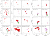 |
Fig. 14 From top to bottom rows: [C/Fe] vs. [N/Fe], [O/Fe] vs. [Na/Fe], and [Mg/Fe] vs. [Al/Fe] diagrams of the anomalous GCs in our sample with available spectroscopy. 1P and 2P stars are represented by the dim green and violet dots, while anomalous stars are represented in red. The iron-rich population of NGC 7089 (see text) is indicated with orange starred symbols. |
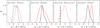 |
Fig. 16 Kernel density distribution of the [C+N+O/Fe] values of NGC 0362, NGC 1851, ωCen, and NGC 6656. The distribution of canonical and anomalous stars is shown in black and red, respectively. Median spectroscopic errors are represented in gray. For NGC 0362, which has only one anomalous star, its position is highlighted with a vertical red line. The narrow distribution of canonical stars in NGC 5139 (Marino et al. 2012 dataset) is due to having only two stars with ChM tagging. |
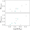 |
Fig. 17 [Fe/H], [Ba/Fe], and [C+N+O/Fe] width of Type II GCs in our sample vs. their mass (in upper, central, and lower panel, respectively). Cyan dots indicate clusters for which the width has been measured using fewer than ten stars (see text for details). |
Acknowledgements
This work has been funded by the European Union – NextGenerationEU RRF M4C2 1.1 (PRIN 2022 2022MMEB9W: “Understanding the formation of globular clusters with their multiple stellar generations”, CUP C53D23001200006). T. Ziliotto acknowledges funding from the European Union’s Horizon 2020 research and innovation programme under the Marie Skłodowska-Curie Grant Agreement No. 101034319 and from the “European Union – NextGenerationEU”. S.J. acknowledges support from the NRF of Korea (2022R1A2C3002992, 2022R1A6A1A03053472).
Appendix A details on our dataset
In this appendix, we provide additional details about our dataset. Figure A.1 presents all previously published ChMs based on HST photometry used in this work. The ChMs of NGC 6402 and NGC 2419 are sourced from D’Antona et al. (2022) and Zennaro et al. (2019), respectively, while the remaining data come from Milone et al. (2017). Similarly, Figure A.2 shows the ChMs published by Jang et al. (2022), which utilize UBVI photometry from ground-based facilities. In both figures, stars with available spectroscopy measurements from the literature are marked with green, violet, and red dots, corresponding to their belonging to the 1P,2P, and anomalous populations, respectively. The stars associated with the remnant of the host galaxy of NGC 7089 are indicated with orange starred symbols. While in the HST-based ChM their separation from the bulk of anomalous stars is evident, in the ChM from Jang and collaborators, based on a smaller color scale on the ChM x-axis, the separation is not clear-cut. To separate the two populations, we rely on their large [Fe/H] differences (Yong et al. 2014), tagging with orange starred symbols the stars with [Fe/H] larger than -1.2 dex.
At the same signal-to-noise ratio, the separation between different populations on the ChM becomes less clear-cut when considering stars in the most metal-poor GCs. In particular, this effect is more prominent in the UBVI photometric system compared to others that have filters that more efficiently cover the crucial absorption bands to disentangle multiple populations, like the HST WFC3 or the JWL indices (e. g., Lee 2017). For example, as pointed out by Lee (2024), the separation between populations in ChMs made with the UBVI bands tends to become less clear-cut, as the CN absorption band becomes weaker when considering M92 ([Fe/H] ~ − 2.3). For GCs in this regime for which we exploited ground-based photometry, we verified that the ΔX derived relying on the UBVI ChM is in agreement within uncertainties with ΔX obtained through the more robust HST tagging, thus showing how any possible limitation among metal-poor GCs does not significantly affect our results.
Table A.1 summarizes the complete dataset used in this work. For each GC, we list the source studies and the number of stars with ChM tagging (from both HST and ground-based photometry) for each of the 14 species included in our analysis.
Figures A.3, A.4, and A.5, illustrate the median abundances of 1P, 2P, and (when present) anomalous stars for each dataset covered in Section 3.2, selecting only those with at least four stars per population. In these plots, open circles represent the median abundance value for each population on the y-axis, while the x-axis positions are arbitrarily adjusted to display 1P, 2P, and anomalous stars from left to right. Grey lines connect median values from the same study. The APOGEE dataset measurements, which covers the largest number of common stars, element abundances, and clusters, are highlighted with open squares. Each point is accompanied by a colored rectangular band representing the interquartile range of the abundance distribution, according to the corresponding population.
With over 50 spectroscopic studies considered, systematic errors and disagreements in element abundances across studies are unavoidable. Indeed, we are dealing with different works, each using instruments with varying resolutions, distinct spectral features, and different data reduction techniques, thus making it inevitable to encounter systematic biases in abundance ratios measured across separate studies. To mitigate these effects, our analysis relies exclusively on relative metrics, such as Δ and W. Since systematic errors typically shift the entire abundance scale uniformly, our approach effectively mitigates their impact. We emphasize that absolute abundance measurements are never combined in our analysis. Instead, we calculate Δ and W independently for each dataset and then average these quantities across the datasets. The only exception occurs in Section 5, where we combine [Fe/H] measurements from multiple datasets to compare them to the x-axis position on the ChM (Figure 10). However, since [Fe/H] is one of the most extensively measured elements in spectroscopy, we were able to leverage a large sample of stars measured in multiple studies whenever combining datasets. This allowed us to robustly estimate and account for any potential systematics.
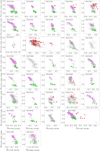 |
Fig. A.1 ΔCF275W,F336W,F438W vs. ΔF275W,F814W ChM from Milone et al. (2017). The ChM of NGC 6402 comes from D’Antona et al. (2022), while the ΔCF275W,F336W,F438W vs. ΔF438W,F814W was published by Zennaro et al. (2019). Stars with spectroscopy abundances are highlighted with the color-code introduced in Figure 1. |
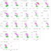 |
Fig. A.2 Same as Figure A.1 but for the ΔCU,B,I vs. ΔB,I ChM from Jang et al. (2022) of the GCs in our sample. |
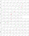 |
Fig. A.3 Median abundances (open dots) of lithium, carbon, nitrogen, oxygen, sodium, and magnesium for the different populations identified in our sample of GCs with at least four stars with both photometric tagging and spectroscopic abundances. The open squares highlight APOGEE measurements. The vertical bands represent the interquartile range, and are color coded following the prescriptions introduced in Figure 1. Median values from the same spectroscopic dataset are connected by gray lines. |
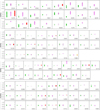 |
Fig. A.4 Same as Figure A.3 but for aluminum, silicon, potassium, and calcium. |
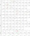 |
Fig. A.5 Same as Figure A.3 but for titanium, iron, nickel, and barium. |
Summary of the spectroscopic datasets used in this work. For each dataset, we report the number of stars with available population tagging from the ChM. The ’−’ symbol indicates the lack of measurements for a given elemental ratio.
Average abundance differences between 1P and 2P stars. The rows indicated with ’A’ are referred to the differences between 1P and anomalous stars. Entries with the ’−’ symbol refers to elements with no measurements. Measurements with the ’*’ notation are based on carbon and nitrogen abundances above the RGB bump.
Appendix B spatial biases
Several GCs exhibit radial gradients in their population fractions, with the proportion of 1P stars increasing towards the outskirts and 2P stars dominating in the central regions (e.g., Dondoglio et al. 2021; Leitinger et al. 2023; Mehta et al. 2025). Spectroscopic observations, however, often avoid the densely crowded central areas of GCs, focusing instead on stars located further out. This observational bias could lead to undersampling of 2P stars in the inner regions. If the fraction of 2P stars decreases towards the core, their overall contribution could be underestimated when measuring the Width, potentially introducing a spatial bias.
To evaluate whether this effect significantly impacts our results, we conducted simulations modeling a realistic sample of 50 stars, a typical number available for Width measurements. Two population distributions were considered: one with a 1P fraction of 0.3 and the other with 0.7, based on estimates reported in the literature. These simulations incorporated three scenarios with differences Δ between the median 1P and 2P abundance values of 0.2, 0.7, and 1.2 dex, which represent typical 1P-2P light-element variations observed in Section 3. Figure B.1 illustrates the simulated distributions for each Δ, shown in the left, central, and right panels, respectively. To mimic real observations, we applied the Width calculation method described in Section 4 and assumed typical spectroscopic measurement errors of 0.15 dex.
In the Δ = 0.2 case, we measured Width values of 0.24±0.06 and 0.20±0.07 for 1P fractions of 0.3 and 0.7, respectively. For Δ = 0.7, the results were 0.84±0.06 and 0.85±0.06, while for Δ = 1.2, the values were 1.26±0.07 and 1.34±0.09. Across all three scenarios, the differences introduced by radial population gradients were negligible. These findings demonstrate that, under realistic observational conditions, spatial biases due to population gradients do not significantly affect our Width measurements. This ensures that our results remain robust and unbiased by the radial distribution of 1P and 2P stars.
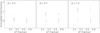 |
Fig. B.1 Simulated distributions of spectroscopic abundances when the 1P fraction is 0.3 and 0.7. Left, central, and right panels represents simulation for Δ = 0.2, 0.7, and 1.2, repsectively (see text for details). |
References
- Abdurro’uf, Accetta, K., Aerts, C., et al. 2022, ApJS, 259, 35 [NASA ADS] [CrossRef] [Google Scholar]
- Aguilera-Gómez, C., Monaco, L., Mucciarelli, A., et al. 2022, A&A, 657, A33 [NASA ADS] [CrossRef] [EDP Sciences] [Google Scholar]
- Alvarez Garay, D. A., Mucciarelli, A., Lardo, C., Bellazzini, M., & Merle, T. 2022, ApJ, 928, L11 [NASA ADS] [CrossRef] [Google Scholar]
- Alvarez Garay, D. A., Mucciarelli, A., Bellazzini, M., Lardo, C., & Ventura, P. 2024, A&A, 681, A54 [NASA ADS] [CrossRef] [EDP Sciences] [Google Scholar]
- Bastian, N., & Lardo, C. 2018, ARA&A, 56, 83 [Google Scholar]
- Baumgardt, H., & Hilker, M. 2018, MNRAS, 478, 1520 [Google Scholar]
- Boberg, O. M., Friel, E. D., & Vesperini, E. 2016, ApJ, 824, 5 [NASA ADS] [CrossRef] [Google Scholar]
- Bragaglia, A., Carretta, E., D’Orazi, V., et al. 2017, A&A, 607, A44 [NASA ADS] [CrossRef] [EDP Sciences] [Google Scholar]
- Buder, S., Kos, J., Wang, E. X., et al. 2024, arXiv e-prints [arXiv:2409.19858] [Google Scholar]
- Cameron, A. G. W., & Fowler, W. A. 1971, ApJ, 164, 111 [NASA ADS] [CrossRef] [Google Scholar]
- Carlos, M., Marino, A. F., Milone, A. P., et al. 2023, MNRAS, 519, 1695 [Google Scholar]
- Carretta, E. 2014, ApJ, 795, L28 [Google Scholar]
- Carretta, E. 2015, ApJ, 810, 148 [Google Scholar]
- Carretta, E., & Bragaglia, A. 2022, A&A, 660, L1 [NASA ADS] [CrossRef] [EDP Sciences] [Google Scholar]
- Carretta, E., & Bragaglia, A. 2023, A&A, 677, A73 [NASA ADS] [CrossRef] [EDP Sciences] [Google Scholar]
- Carretta, E., & Bragaglia, A. 2024, A&A, 690, A158 [NASA ADS] [CrossRef] [EDP Sciences] [Google Scholar]
- Carretta, E., Bragaglia, A., Gratton, R. G., et al. 2007a, A&A, 464, 939 [NASA ADS] [CrossRef] [EDP Sciences] [Google Scholar]
- Carretta, E., Bragaglia, A., Gratton, R. G., Lucatello, S., & Momany, Y. 2007b, A&A, 464, 927 [NASA ADS] [CrossRef] [EDP Sciences] [Google Scholar]
- Carretta, E., Bragaglia, A., Gratton, R. G., et al. 2009, A&A, 505, 117 [NASA ADS] [CrossRef] [EDP Sciences] [Google Scholar]
- Carretta, E., Bragaglia, A., Gratton, R. G., et al. 2010, ApJ, 714, L7 [Google Scholar]
- Carretta, E., Lucatello, S., Gratton, R. G., Bragaglia, A., & D’Orazi, V. 2011, A&A, 533, A69 [NASA ADS] [CrossRef] [EDP Sciences] [Google Scholar]
- Carretta, E., Bragaglia, A., Gratton, R. G., et al. 2013a, A&A, 557, A138 [NASA ADS] [CrossRef] [EDP Sciences] [Google Scholar]
- Carretta, E., Gratton, R. G., Bragaglia, A., D’Orazi, V., & Lucatello, S. 2013b, A&A, 550, A34 [NASA ADS] [CrossRef] [EDP Sciences] [Google Scholar]
- Carretta, E., Bragaglia, A., Gratton, R. G., et al. 2014a, A&A, 564, A60 [NASA ADS] [CrossRef] [EDP Sciences] [Google Scholar]
- Carretta, E., D’Orazi, V., Gratton, R. G., & Lucatello, S. 2014b, A&A, 563, A32 [NASA ADS] [CrossRef] [EDP Sciences] [Google Scholar]
- Carretta, E., Bragaglia, A., Gratton, R. G., et al. 2015, A&A, 578, A116 [CrossRef] [EDP Sciences] [Google Scholar]
- Černiauskas, A., Kučinskas, A., Klevas, J., et al. 2017, A&A, 604, A35 [Google Scholar]
- Charbonnel, C., Brown, J. A., & Wallerstein, G. 1998, A&A, 332, 204 [NASA ADS] [Google Scholar]
- Cohen, J. G., & Kirby, E. N. 2012, ApJ, 760, 86 [Google Scholar]
- Cohen, J. G., Huang, W., & Kirby, E. N. 2011, ApJ, 740, 60 [Google Scholar]
- D’Antona, F., Vesperini, E., D’Ercole, A., et al. 2016, MNRAS, 458, 2122 [Google Scholar]
- D’Antona, F., Ventura, P., Fabiola Marino, A., et al. 2019, ApJ, 871, L19 [Google Scholar]
- D’Antona, F., Milone, A. P., Johnson, C. I., et al. 2022, ApJ, 925, 192 [CrossRef] [Google Scholar]
- Dobrovolskas, V., Kolomiecas, E., Kučinskas, A., Klevas, J., & Korotin, S. 2021, A&A, 656, A67 [NASA ADS] [CrossRef] [EDP Sciences] [Google Scholar]
- Dondoglio, E., Milone, A. P., Lagioia, E. P., et al. 2021, ApJ, 906, 76 [NASA ADS] [CrossRef] [Google Scholar]
- Dondoglio, E., Milone, A. P., Marino, A. F., et al. 2023, MNRAS, 526, 2960 [Google Scholar]
- D’Orazi, V., & Marino, A. F. 2010, ApJ, 716, L166 [Google Scholar]
- D’Orazi, V., Angelou, G. C., Gratton, R. G., et al. 2014, ApJ, 791, 39 [CrossRef] [Google Scholar]
- D’Orazi, V., Gratton, R. G., Angelou, G. C., et al. 2015, MNRAS, 449, 4038 [CrossRef] [Google Scholar]
- Duggan, G. E., Kirby, E. N., Andrievsky, S. M., & Korotin, S. A. 2018, ApJ, 869, 50 [NASA ADS] [CrossRef] [Google Scholar]
- Gerber, J. M., Friel, E. D., & Vesperini, E. 2018, AJ, 156, 6 [Google Scholar]
- Gerber, J. M., Friel, E. D., & Vesperini, E. 2021, AJ, 161, 288 [Google Scholar]
- Gilmore, G., Randich, S., Worley, C. C., et al. 2022, A&A, 666, A120 [NASA ADS] [CrossRef] [EDP Sciences] [Google Scholar]
- Gratton, R., Bragaglia, A., Carretta, E., et al. 2019, A&A Rev., 27, 8 [NASA ADS] [CrossRef] [Google Scholar]
- Gunn, J. E., Siegmund, W. A., Mannery, E. J., et al. 2006, AJ, 131, 2332 [NASA ADS] [CrossRef] [Google Scholar]
- Häberle, M., Neumayer, N., Bellini, A., et al. 2024, ApJ, 970, 192 [Google Scholar]
- Harris, W. E. 1996, AJ, 112, 1487 [Google Scholar]
- Hourihane, A., François, P., Worley, C. C., et al. 2023, A&A, 676, A129 [NASA ADS] [CrossRef] [EDP Sciences] [Google Scholar]
- Jang, S., Milone, A. P., Legnardi, M. V., et al. 2022, MNRAS, 517, 5687 [CrossRef] [Google Scholar]
- Johnson, C. I., & Pilachowski, C. A. 2010, ApJ, 722, 1373 [NASA ADS] [CrossRef] [Google Scholar]
- Johnson, C. I., & Pilachowski, C. A. 2012, ApJ, 754, L38 [NASA ADS] [CrossRef] [Google Scholar]
- Johnson, C. I., Caldwell, N., Rich, R. M., et al. 2017, ApJ, 842, 24 [Google Scholar]
- Johnson, C. I., Caldwell, N., Michael Rich, R., Mateo, M., & Bailey, J. I. 2019, MNRAS, 485, 4311 [Google Scholar]
- Jönsson, H., Holtzman, J. A., Allende Prieto, C., et al. 2020, AJ, 160, 120 [Google Scholar]
- Karakas, A. I., & Lattanzio, J. C. 2014, PASA, 31, e030 [NASA ADS] [CrossRef] [Google Scholar]
- Kirby, E. N., Guhathakurta, P., Zhang, A. J., et al. 2016, ApJ, 819, 135 [NASA ADS] [CrossRef] [Google Scholar]
- Kolomiecas, E., Dobrovolskas, V., Kučinskas, A., Bonifacio, P., & Korotin, S. 2022, A&A, 660, A46 [NASA ADS] [CrossRef] [EDP Sciences] [Google Scholar]
- Kovalev, M., Bergemann, M., Ting, Y.-S., & Rix, H.-W. 2019, A&A, 628, A54 [NASA ADS] [CrossRef] [EDP Sciences] [Google Scholar]
- Lagioia, E. P., Milone, A. P., Legnardi, M. V., et al. 2025, ApJ, 979, 30 [Google Scholar]
- Lardo, C., Salaris, M., Cassisi, S., & Bastian, N. 2022, A&A, 662, A117 [NASA ADS] [CrossRef] [EDP Sciences] [Google Scholar]
- Lee, J.-W. 2017, ApJ, 844, 77 [NASA ADS] [CrossRef] [Google Scholar]
- Lee, J.-W. 2022, ApJS, 263, 20 [NASA ADS] [CrossRef] [Google Scholar]
- Lee, J.-W. 2023, ApJ, 950, L6 [Google Scholar]
- Lee, J.-W. 2024, ApJ, 961, 227 [NASA ADS] [CrossRef] [Google Scholar]
- Lee, J.-W., & Sneden, C. 2021, ApJ, 909, 167 [NASA ADS] [CrossRef] [Google Scholar]
- Lee, J.-W., Kim, T.-H., Kim, H.-S., et al. 2025, AJ, 169, 143 [Google Scholar]
- Legnardi, M. V., Milone, A. P., Armillotta, L., et al. 2022, MNRAS, 513, 735 [NASA ADS] [CrossRef] [Google Scholar]
- Leitinger, E., Baumgardt, H., Cabrera-Ziri, I., Hilker, M., & Pancino, E. 2023, MNRAS, 520, 1456 [NASA ADS] [CrossRef] [Google Scholar]
- Marino, A. F., Villanova, S., Piotto, G., et al. 2008, A&A, 490, 625 [NASA ADS] [CrossRef] [EDP Sciences] [Google Scholar]
- Marino, A. F., Milone, A. P., Piotto, G., et al. 2009, A&A, 505, 1099 [CrossRef] [EDP Sciences] [Google Scholar]
- Marino, A. F., Milone, A. P., Piotto, G., et al. 2011, ApJ, 731, 64 [Google Scholar]
- Marino, A. F., Milone, A. P., Piotto, G., et al. 2012, ApJ, 746, 14 [CrossRef] [Google Scholar]
- Marino, A. F., Milone, A. P., Karakas, A. I., et al. 2015, MNRAS, 450, 815 [NASA ADS] [CrossRef] [Google Scholar]
- Marino, A. F., Milone, A. P., Renzini, A., et al. 2019a, MNRASz, 487, 3815 [Google Scholar]
- Marino, A. F., Milone, A. P., Sills, A., et al. 2019b, ApJ, 887, 91 [NASA ADS] [CrossRef] [Google Scholar]
- Marino, A. F., Milone, A. P., Renzini, A., et al. 2021, ApJ, 923, 22 [CrossRef] [Google Scholar]
- Marino, A. F., Milone, A. P., Dondoglio, E., et al. 2023, ApJ, 958, 31 [NASA ADS] [CrossRef] [Google Scholar]
- Masseron, T., García-Hernández, D. A., Mészáros, S., et al. 2019, A&A, 622, A191 [NASA ADS] [CrossRef] [EDP Sciences] [Google Scholar]
- Mastrobuono-Battisti, A., & Perets, H. B. 2016, ApJ, 823, 61 [Google Scholar]
- McKenzie, M., Yong, D., Marino, A. F., et al. 2022, MNRAS, 516, 3515 [NASA ADS] [CrossRef] [Google Scholar]
- Mehta, V. J., Milone, A. P., Casagrande, L., et al. 2025, MNRAS, 536, 1077 [Google Scholar]
- Mészáros, S., Masseron, T., García-Hernández, D. A., et al. 2020, MNRAS, 492, 1641 [Google Scholar]
- Milone, A. P., & Marino, A. F. 2022, Universe, 8, 359 [NASA ADS] [CrossRef] [Google Scholar]
- Milone, A. P., Piotto, G., Bedin, L. R., et al. 2012, ApJ, 744, 58 [NASA ADS] [CrossRef] [Google Scholar]
- Milone, A. P., Marino, A. F., Dotter, A., et al. 2014, ApJ, 785, 21 [NASA ADS] [CrossRef] [Google Scholar]
- Milone, A. P., Marino, A. F., Piotto, G., et al. 2015, MNRAS, 447, 927 [NASA ADS] [CrossRef] [Google Scholar]
- Milone, A. P., Piotto, G., Renzini, A., et al. 2017, MNRAS, 464, 3636 [Google Scholar]
- Milone, A. P., Marino, A. F., Renzini, A., et al. 2018, MNRAS, 481, 5098 [NASA ADS] [CrossRef] [Google Scholar]
- Mucciarelli, A., Salaris, M., Lovisi, L., et al. 2011, MNRAS, 412, 81 [NASA ADS] [CrossRef] [Google Scholar]
- Mucciarelli, A., Bellazzini, M., Ibata, R., et al. 2012, MNRAS, 426, 2889 [Google Scholar]
- Mucciarelli, A., Bellazzini, M., Merle, T., et al. 2015, ApJ, 801, 68 [Google Scholar]
- Mucciarelli, A., Dalessandro, E., Massari, D., et al. 2016, ApJ, 824, 73 [NASA ADS] [CrossRef] [Google Scholar]
- Mucciarelli, A., Merle, T., & Bellazzini, M. 2017, A&A, 600, A104 [NASA ADS] [CrossRef] [EDP Sciences] [Google Scholar]
- Mucciarelli, A., Salaris, M., Monaco, L., et al. 2018, A&A, 618, A134 [NASA ADS] [CrossRef] [EDP Sciences] [Google Scholar]
- Pasquini, L., Avila, G., Blecha, A., et al. 2002, The Messenger, 110, 1 [Google Scholar]
- Pancino, E., Romano, D., Tang, B., et al. 2017, A&A, 601, A112 [NASA ADS] [CrossRef] [EDP Sciences] [Google Scholar]
- Randich, S., Gilmore, G., Magrini, L., et al. 2022, A&A, 666, A121 [NASA ADS] [CrossRef] [EDP Sciences] [Google Scholar]
- Schiappacasse-Ulloa, J., Lucatello, S., Rain, M. J., & Pietrinferni, A. 2022, MNRAS, 511, 231 [NASA ADS] [CrossRef] [Google Scholar]
- Sheinis, A., Anguiano, B., Asplund, M., et al. 2015, J. Astron. Telesc. Instrum. Syst., 1, 035002 [NASA ADS] [CrossRef] [Google Scholar]
- Shetrone, M., Tayar, J., Johnson, J. A., et al. 2019, ApJ, 872, 137 [NASA ADS] [CrossRef] [Google Scholar]
- Siegel, M. H., Dotter, A., Majewski, S. R., et al. 2007, ApJ, 667, L57 [NASA ADS] [CrossRef] [Google Scholar]
- Stetson, P. B., Pancino, E., Zocchi, A., Sanna, N., & Monelli, M. 2019, MNRAS, 485, 3042 [Google Scholar]
- Tailo, M., Milone, A. P., Lagioia, E. P., et al. 2020, MNRAS, 498, 5745 [CrossRef] [Google Scholar]
- Tautvaišienė, G., Drazdauskas, A., Bragaglia, A., et al. 2022, A&A, 658, A80 [CrossRef] [EDP Sciences] [Google Scholar]
- Ventura, P., D’Antona, F., Di Criscienzo, M., et al. 2012, ApJ, 761, L30 [Google Scholar]
- Yong, D., & Grundahl, F. 2008, ApJ, 672, L29 [NASA ADS] [CrossRef] [Google Scholar]
- Yong, D., Roederer, I. U., Grundahl, F., et al. 2014, MNRAS, 441, 3396 [NASA ADS] [CrossRef] [Google Scholar]
- Yong, D., Grundahl, F., & Norris, J. E. 2015, MNRAS, 446, 3319 [NASA ADS] [CrossRef] [Google Scholar]
- Zennaro, M., Milone, A. P., Marino, A. F., et al. 2019, MNRAS, 487, 3239 [CrossRef] [Google Scholar]
See documentation https://www.sdss4.org/dr17/ for details.
In our study of NGC 1851, we choose to utilize the ChMs provided by Milone et al. (2017) and Jang et al. (2022) over the more recent developed by Dondoglio et al. (2023) because of their wider magnitude coverage, which suits our goal of tagging a larger number of stars.
When considering spectroscopic estimates from different works, it is unavoidable to deal with systematics between the various datasets. However, ΔX is measured by subtracting median abundances of stars from the same dataset (therefore affected by the same systematics), thus erasing any systematics.
The lithium abundance in RGB stars below the bump is not primordial but has been depleted due to the first dredge-up in the RGB phase (e.g., Karakas & Lattanzio 2014). Different populations may experience varying degrees of lithium depletion depending on their stellar parameters. However, Schiappacasse-Ulloa et al. (2022) observed the same A(Li) vs. [Al/Fe] anticorrelation in MS turn-off and RGB stars, indicating that evolutionary lithium depletion has minimal or undetectable impact on the 1P-2P Li trend in the lower RGB phase.
The mass of GCs is taken from Baumgardt & Hilker (2018), while the overall [Fe/H] come from Harris (1996, 2010 edition). We assume [Fe/H] as a tracer of the star overall metals’ abundances.
All Tables
Summary of the spectroscopic datasets used in this work. For each dataset, we report the number of stars with available population tagging from the ChM. The ’−’ symbol indicates the lack of measurements for a given elemental ratio.
Average abundance differences between 1P and 2P stars. The rows indicated with ’A’ are referred to the differences between 1P and anomalous stars. Entries with the ’−’ symbol refers to elements with no measurements. Measurements with the ’*’ notation are based on carbon and nitrogen abundances above the RGB bump.
All Figures
|
Fig. 1 Left panels: from left to right, ΔCF275W,F336W,F438W vs. ΔF275W,F814W HST ChMs of NGC 5904 and NGC 1851. 1P, 2P, and anomalous stars with available spectroscopy measurements are highlighted with green, violet, and red dots, respectively. Right panels: as per left panels but with the ground-based ΔCU,B,I vs. ΔB,I ChM. |
| In the text | |
|
Fig. 2 Summary of the photometric diagrams introduced in Section 3.1. Panel (a1) and (a2): two-color diagram of mF275W-mF336W vs. mF336W-mF438W and CU,B,I vs. B − I pseudo two-color diagram for the red HB of NGC 5927. Panel (b): ΔCU,B,I vs. ΔU,B ChM of NGC 5286. Panel (c): same but for NGC 6656. Panel (d): ΔCF275W,F336W,F435W vs. ΔF275W,F814W ChM of ωCen derived from the catalog by Häberle et al. (2024). Green, violet, and red dots represent 1P, 2P, and anomalous stars, respectively. |
| In the text | |
|
Fig. 3 Differences in median abundances of A(Li), [C/Fe], [N/Fe], [O/Fe], and [Na/Fe] between 1P and 2P stars (violet) and 1P and anomalous (red) stars. The green lines separate the regime where 2P and anomalous stars are enriched or depleted (see text for details). The y-axis scale is adjusted in each plot to optimize clarity. The smaller dots indicate GCs where the Δ[C/Fe] and Δ[N/Fe] measurements are derived from RGB stars brighter than the bump. |
| In the text | |
|
Fig. 4 Differences in median abundances of [Mg/Fe], [Al/Fe], [Si/Fe], [K/Fe], and [Ca/Fe] between 1P and 2P stars (violet) and 1P and anomalous stars (red). Symbols and lines follow the same conventions as in Figure 3. The orange starred symbol refers to the host galaxy remnant of NGC 7089. |
| In the text | |
|
Fig. 5 Differences in median abundances of [Ti/Fe], [Fe/H], [Ni/Fe], and [Ba/Fe] between 1P and 2P stars (violet) and 1P and anomalous stars (red). Symbols and lines follow the same conventions as in Figure 3. |
| In the text | |
|
Fig. 6 Upper panels: difference between the median of the 2P and 1P abundance of each analyzed element. Positive and negative values (above and below the green line), represent enrichment and depletion of 2P stars, respectively. The right panel displays the 2P–1P helium difference (in mass fraction) from Milone et al. (2018). Lower panels: diagrams of Δ[N/Fe] vs. Δ[C/Fe] (left), Δ[Na/Fe] vs. Δ[O/Fe] (middle), and Δ[Al/Fe] vs. Δ[Mg/Fe] (right). Each point is color coded according to their [Fe/H], following the scheme represented in the color bar. Smaller dots indicate Δ[C/Fe] and Δ[N/Fe] based on RGB stars above the bump. |
| In the text | |
|
Fig. 7 Total spread of [C/Fe], [N/Fe], [O/Fe], [Na/Fe], [Mg/Fe], [Al/Fe], [Si/Fe], [K/Fe], [Ca/Fe], [Ti/Fe], [Fe/H], and [Ni/Fe] with respect to the clusters’ mass and average metallicity. In each plot, we report the Spearman correlation coefficient, with its significance (p-value) in round parentheses. Gray points are relative to W[C/Fe] and W[C/Fe] measurements based on stars below the RGB bump. |
| In the text | |
|
Fig. 8 Panels (a1) and (a2): WC,N,O,Na vs. log(M/M⊙) and [Fe/H], respectively. Panels (b1) and (b2): same as panels (a1) and (a2) but for WMg,Al. GCs within the 5.5 < log(M/M⊙) < 5.9 mass interval used to remove the metallicity dependence (see text for details) are encircled in yellow. Panel (b3): resulting width after removing [Fe/H] dependence (ΔWMg,Al) vs. mass. Panels (c1) and (c2): total width of light elements involved in the multiple population phenomenon WC,N,O,Na,Mg,Al vs. mass and maximum helium spread measured by Milone et al. (2018), respectively. The Spearman correlation coefficient and its p-value are reported in each plot as in Figure 7. |
| In the text | |
|
Fig. 9 Left panel: 1P stars [Fe/H] spread from spectroscopy |
| In the text | |
|
Fig. 10 [Fe/H] abundance for 1P stars vs. ΔF275W,F814W and/or ΔU,I (depending on the availability of iron spectroscopic measurements) of NGC 0104, NGC 1261, NGC 3201, NGC 4833, NGC 5272, NGC 5904, NGC 6254, and NGC 6715. Grey lines indicate the best-fit straight line. Correlation coefficients are reported in each plot. Comparison of iron abundances with HST and ground-based x-axis of the ChMs are aligned along the even and odd columns on the image, respectively. |
| In the text | |
|
Fig. 11 Same as Figure 10 but for logϵ(α) vs. ΔF275W,F814W (only for NGC 0104) and ΔU,I for NGC 0104, NGC 1261, NGC 3201, NGC 5272, NGC 5904, and NGC 6254. |
| In the text | |
|
Fig. 12 The y-axis of the ChM vs. A(Li). Measurements and upper limit (arrows) are color coded according to their population. For each GC, the bottom panel refers to stars in the innermost areas covered by HST observations, while the upper ChM regards stars outside the central field (covered by ground-based photometry in all GCs except ωCen). Horizontal blue and red dashed lines indicate the 70-th percentile level of the 1P+2P and 1P+anomalous star distributions, respectively. Above the ChMs, starred green and blue symbols denote the median 1P and 2Pext A(Li), shifted arbitrarily on the y-axis for illustration purposes. |
| In the text | |
|
Fig. 13 Difference between lithium abundances for the most extreme 2P stars and the 1P stars (open black dots) vs. the cluster mass and maximum helium spread (right and left panels, respectively). Red crosses indicate the same quantity but measured for anomalous stars (see text for details). |
| In the text | |
|
Fig. 14 From top to bottom rows: [C/Fe] vs. [N/Fe], [O/Fe] vs. [Na/Fe], and [Mg/Fe] vs. [Al/Fe] diagrams of the anomalous GCs in our sample with available spectroscopy. 1P and 2P stars are represented by the dim green and violet dots, while anomalous stars are represented in red. The iron-rich population of NGC 7089 (see text) is indicated with orange starred symbols. |
| In the text | |
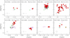 |
Fig. 15 Same as Figure 14 but for the [Ba/Fe] vs. [Fe/H] relation. |
| In the text | |
|
Fig. 16 Kernel density distribution of the [C+N+O/Fe] values of NGC 0362, NGC 1851, ωCen, and NGC 6656. The distribution of canonical and anomalous stars is shown in black and red, respectively. Median spectroscopic errors are represented in gray. For NGC 0362, which has only one anomalous star, its position is highlighted with a vertical red line. The narrow distribution of canonical stars in NGC 5139 (Marino et al. 2012 dataset) is due to having only two stars with ChM tagging. |
| In the text | |
|
Fig. 17 [Fe/H], [Ba/Fe], and [C+N+O/Fe] width of Type II GCs in our sample vs. their mass (in upper, central, and lower panel, respectively). Cyan dots indicate clusters for which the width has been measured using fewer than ten stars (see text for details). |
| In the text | |
|
Fig. A.1 ΔCF275W,F336W,F438W vs. ΔF275W,F814W ChM from Milone et al. (2017). The ChM of NGC 6402 comes from D’Antona et al. (2022), while the ΔCF275W,F336W,F438W vs. ΔF438W,F814W was published by Zennaro et al. (2019). Stars with spectroscopy abundances are highlighted with the color-code introduced in Figure 1. |
| In the text | |
|
Fig. A.2 Same as Figure A.1 but for the ΔCU,B,I vs. ΔB,I ChM from Jang et al. (2022) of the GCs in our sample. |
| In the text | |
|
Fig. A.3 Median abundances (open dots) of lithium, carbon, nitrogen, oxygen, sodium, and magnesium for the different populations identified in our sample of GCs with at least four stars with both photometric tagging and spectroscopic abundances. The open squares highlight APOGEE measurements. The vertical bands represent the interquartile range, and are color coded following the prescriptions introduced in Figure 1. Median values from the same spectroscopic dataset are connected by gray lines. |
| In the text | |
|
Fig. A.4 Same as Figure A.3 but for aluminum, silicon, potassium, and calcium. |
| In the text | |
|
Fig. A.5 Same as Figure A.3 but for titanium, iron, nickel, and barium. |
| In the text | |
|
Fig. B.1 Simulated distributions of spectroscopic abundances when the 1P fraction is 0.3 and 0.7. Left, central, and right panels represents simulation for Δ = 0.2, 0.7, and 1.2, repsectively (see text for details). |
| In the text | |
Current usage metrics show cumulative count of Article Views (full-text article views including HTML views, PDF and ePub downloads, according to the available data) and Abstracts Views on Vision4Press platform.
Data correspond to usage on the plateform after 2015. The current usage metrics is available 48-96 hours after online publication and is updated daily on week days.
Initial download of the metrics may take a while.