| Issue |
A&A
Volume 678, October 2023
|
|
|---|---|---|
| Article Number | A155 | |
| Number of page(s) | 13 | |
| Section | Galactic structure, stellar clusters and populations | |
| DOI | https://doi.org/10.1051/0004-6361/202347189 | |
| Published online | 18 October 2023 | |
Multiple stellar populations found outside the tidal radius of NGC 1851 via Gaia DR3 XP spectra
1
Istituto Nazionale di Astrofisica – Osservatorio Astronomico di Padova, Vicolo dell’Osservatorio 5, 35122 Padova, Italy
e-mail: This email address is being protected from spambots. You need JavaScript enabled to view it.
2
Istituto Nazionale di Astrofisica – Osservatorio Astrofisico di Arcetri, Largo Enrico Fermi, 5, Firenze, 50125 Firenze, Italy
3
Dipartimento di Fisica e Astronomia “Galileo Galilei”, Univ. di Padova, Vicolo dell’Osservatorio 3, 35122 Padova, Italy
4
Center for Galaxy Evolution Research and Department of Astronomy, Yonsei University, Seoul 03722, Korea
Received:
14
June
2023
Accepted:
8
August
2023
Abstract
Aims. Ancient galactic globular clusters (GCs) have long fascinated astronomers due to their intriguing multiple stellar populations (MPs), which are characterized by variations in light element abundances. Among these clusters, type II GCs stand out as they exhibit stars with large differences in heavy-element chemical abundances. These enigmatic clusters, comprising approximately 17% of analyzed GCs with MPs, have been hypothesized to be the remnants of accreted dwarf galaxies.
Methods. We focus on one of the most debated type II GCs, namely, NGC 1851, to investigate its MPs across a wide spatial range of up to 50 arcmin from the cluster center. By using Gaia Data Release 3 low-resolution XP spectra, we generated synthetic photometry to perform a comprehensive analysis of the spatial distribution and kinematics of the canonical and anomalous populations within this GC. By using appropriate color-magnitude diagrams from the synthetic photometry in the BVI bands and in the f41525 band introduced in this work, we identified distinct stellar sequences associated with different heavy-element chemical compositions.
Results. Our results suggest that the canonical and the anomalous populations reside both inside and outside the tidal radius of NGC 1851, up to a distance that exceeds its tidal radius 3.5 times. However, about 80% of stars outside the tidal radius are consistent with characteristics that class them among the canonical population, emphasizing its dominance in the cluster’s outer regions. Remarkably, canonical stars exhibit a more circular on-sky morphology, while the anomalous population displays an elliptical shape. Furthermore, we delve into the kinematics of the multiple populations, examining velocity dispersions, rotation patterns, and potential substructures. Our results reveal a flat or increasing velocity dispersion profile in the outer regions. Additionally, we observe hints of a tangentially anisotropic motion in the outer regions, indicating a preference for stars to escape on radial orbits. Our work demonstrates the capability of synthetic photometry, based on Gaia spectra, to explore multiple populations across the entire cluster field.
Key words: techniques: photometric / surveys / stars: abundances / globular clusters: individual: NGC 1851 / Galaxy: kinematics and dynamics
© The Authors 2023
 Open Access article, published by EDP Sciences, under the terms of the Creative Commons Attribution License (https://creativecommons.org/licenses/by/4.0), which permits unrestricted use, distribution, and reproduction in any medium, provided the original work is properly cited.
This article is published in open access under the Subscribe to Open model. This email address is being protected from spambots. You need JavaScript enabled to view it. to support open access publication.
1. Introduction
Numerous photometric and spectroscopic studies have established the presence of multiple stellar populations (MPs) in Galactic globular clusters (GCs). Type I GCs1, which account for roughly 83% of the 58 GCs investigated by Milone et al. (2017) using multiband UV-optical Hubble Space Telescope (HST) photometry, exhibit variations in light element abundances, such as carbon, oxygen, nitrogen, and sodium. Stars with different light element abundances are commonly referred to as 1P/2P or 1G/2G. Conversely, type II or anomalous GCs, which constitute the remaining 17% of the clusters, exhibit internal variations in both light and heavy elements, such as elements associated with s-processes and metallicity (Marino et al. 2019). Specifically, stars can be grouped into canonical and anomalous stars based on their heavy-element content, with the latter being more metal-rich than the former. Despite numerous studies, the detailed formation process of MPs in GCs remains unclear and none of the proposed scenarios can fully account for the observational constraints (see Bastian & Lardo 2018; Milone & Marino 2022, for recent reviews).
One hypothesis for the origin of light-elements variations suggests that 2P stars were formed from the ejecta of more massive 1P stars after the gas collapsed in the cluster center, creating a more centrally concentrated environment. This scenario is supported by studies such as Decressin et al. (2007), D’Ercole et al. (2010), Denissenkov & Hartwick (2014), and Renzini et al. (2022). Alternatively, another hypothesis suggests that GCs host only a single generation of stars, and stars with different chemical compositions result from specific exotic physical phenomena of proto-GCs, as proposed by studies such as Bastian et al. (2013) and Gieles et al. (2018). Noticeably, the formation of the more complexes type II clusters has also been associated with the nuclear remnants of accreted dwarf galaxies. The broader implication is that these stellar systems would be somehow related to the satellites accreted by the Milky Way during its formation. Indeed, as shown by Milone et al. (2020), the location of these peculiar clusters in the integral space of motions is consistent with most of them being associated with the Gaia Enceladus structure (Helmi et al. 2018). Hence, the characterization and understanding of type II GCs would play a crucial role in the context of Milky Way formation and evolution.
Among type II GCs, NGC 1851 represents one of the most investigated and debated clusters. Indeed, over the last two decades numerous literature photometric and spectroscopic works attempted a detailed characterization of the properties of the canonical and anomalous stellar populations. However, there is still no agreement on the origin of the puzzling anomalous population. Specifically, it is not clear whether canonical and anomalous stars differ in total C+N+O abundances, s-elements content, metallicity and/or age (see e.g., Milone et al. 2008; Cassisi et al. 2008; Ventura et al. 2009; Yong et al. 2009, 2015; Carretta et al. 2010; Marino et al. 2014; Simpson et al. 2017; Tautvaišienė et al. 2022).
An intriguing feature of NGC 1851 is provided by the presence of a stellar halo encircling the cluster and extending up to more than 500 pc from its center, which was first reported by Olszewski et al. (2009), and then confirmed by several other analyses (Sollima et al. 2012; Kuzma et al. 2018; Carballo-Bello et al. 2018; Shipp et al. 2018). Additionally, some studies (see, e.g., Shipp et al. 2018) have detected possible evidence of tidal tails aligned with NGC 1851’s orbit, implying potential tidal stripping due to interactions with the Milky Way. Marino et al. (2014) utilized high-resolution spectroscopic observations, and photometric data to delve into the intricate nature of NGC 1851 and its halo. Intriguingly, through an analysis of the chemical abundances of the s-process elements Sr and Ba, Marino et al. (2014) determined that all the seven studied extra-tidal stars exhibited consistency with s-normal stars, namely, the canonical stellar population observed within NGC 1851. This discovery posed fascinating questions regarding the genesis of these halo stars and their connection to the primary cluster population.
The intricate nature of the combined NGC 1851 cluster and its surrounding halo suggests the possibility of a scenario involving a tidally-disrupted dwarf galaxy, within which NGC 1851 was originally embedded. A similar idea was suggested by Bekki & Yong (2012), who outlined a dynamically plausible scenario with two GCs in a dwarf galaxy merging and forming a new nuclear star cluster surrounded by field stars of the host dwarf. The host dwarf galaxy is stripped through tidal interaction with the Milky Way, leaving behind the stellar nucleus, which is observed as NGC 1851.
Regardless of the efforts in the field, the origin of the anomalous stellar population of NGC 1851 remains concealed. We consider whether it was the result of a merging or the result of peculiar star formation processes. The answer to these questions may reside among stars beyond the tidal tail of the cluster. Indeed, in the context of the formation of MPs, the properties of the stars in the cluster outskirts may provide the smoking gun to disentangle between different formation scenarios, as they could still retain the imprint of the physical processes that shape GCs. However, despite the crucial constraints that the analysis of chemical abundances among extra-tidal stars of GCs can provide, these studies have been difficult to carry out. The main challenge is to observe a sizable number of stars in the outskirt regions that are associated with the cluster and that are bright enough to make spectroscopic analysis of chemical abundances feasible.
In this work, we introduce a new approach to extend the study of the canonical and anomalous stellar populations in NGC 1851 and, for the first time, we investigate the chemical and dynamical properties of extra-tidal stars in NGC 1851. Remarkably, the recent publication of Gaia Data Release 3 (DR3, Gaia Collaboration 2023b) and Gaia BP − RP spectra (hereafter, XP spectra, Montegriffo et al. 2023; De Angeli et al. 2023) allows us to take the study of MPs in GCs to a next level. Indeed, thanks to Gaia DR3 XP spectra, currently available for ∼220 million sources brighter than G = 17.5, we have the opportunity to generate synthetic photometry in virtually any photometric systems for all the stars observed by Gaia. In the context of Galactic GCs, this offers an unparalleled opportunity. While HST photometry is limited to the innermost cluster regions, approximately within 1.5 arcmin, and ground-based observations typically extend up to around 15–20 arcmin from the cluster center, Gaia DR3 XP spectra enable us to explore BVI synthetic photometry across the entire cluster field. This allows for the investigation of MPs spanning from the innermost regions to the relatively unexplored tidal radii and beyond. Notably, our novel approach discussed in this study allows us to study MPs up to approximately 60 arcmin from the cluster center, thereby significantly extending our understanding of the cluster’s population distribution.
The paper is organized as follows. In Sect. 2, we discuss the data preparation, cluster member selection. In Sect. 3, we present the clusters’ color-magnitude diagrams (CMDs) with their multiple populations. The analysis of the morphology and dynamics of MPs is carried out in Sect. 4. Finally, Sect. 5 offers a discussion and summary of the results.
2. Data preparation
In order to build CMDs suited for the investigation of different stellar populations in type II GCs, we need high-quality photometry in multiple filters. Different filter combinations can indeed reveal the presence of MPs with distinct light and heavy element abundances. In particular, the index CBVI = (B − V)−(V − I) have been shown to effectively separate stellar populations with different heavy element and overall C+N+O content among bright RGB stars (Marino et al. 2015). Thus, it is suited to investigate the properties of canonical and anomalous stars in type II GCs (e.g., Marino et al. 2015)2.
Thanks to the exquisite data provided by Gaia DR3, we are able to build different synthetic pseudo-colors to investigate MPs in GCs. In the following, we describe our procedure to select bona fide cluster members and to build appropriate CMDs in the type II GC NGC 1851. Specifically, we exploit the synthetic CBVI pseudo-color to identify and investigate canonical and anomalous stars up to ∼45 arcmin from the cluster centers, namely, far beyond the tidal radius, namely 11.7 arcmin3. Hence, we study the halo of stars surrounding NGC 1851 and compare the properties of the different stellar populations.
2.1. Selection of cluster members
To investigate the properties and kinematics of MPs in GCs we need to (i) identify stars with accurate astrometric and photometric measurements and (ii) disentangle cluster members from field stars contaminants. To achieve this goal, we adapted the method discussed in Milone et al. (2018), Cordoni et al. (2020a,b, 2023). The results of the selection process are shown in Fig. 1 for the GC NGC 1851. Moreover, we exploited different Gaia DR3 photometric and astrometric parameters, and the quality selection criteria discussed in Riello et al. (2018, 2021), Gaia Collaboration (2023a). The adopted quality criteria are the following: (i) RUWE < 1.4, (ii) IPD_frac_multi_peak < 7, (iii) IPD_frac_odd_win < 7, (iv) |C*|< σC* (see e.g., Sect. 9.2 in Riello et al. 2021), and (v) ϵμ < 0.1 mas yr−1, where ϵμ is defined in Lindegren et al. (2018):
 (1)
(1)
 (2)
(2)
 (3)
(3)
 (4)
(4)
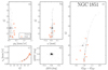 |
Fig. 1. Cluster members selection. Panel a: proper motion distance (μR) relative to NGC 1851 mean motion derived in Vasiliev & Baumgardt (2021), as a function of Gaia G magnitude. Cluster members are displayed as black shaded points, while residual field stars contaminants are shown with orange crosses. Panel b: parallax (ω) as a function of G magnitude. Panel c: uncertainty in proper motions (ϵμ) vs. Gaia G magnitude. Panel d: Δ RA vs. Δ Dec of the selected cluster members. Panel e: G vs. GBP − GRP CMD of the selected cluster members. |
and is shown in Fig. 1c. We applied constraints (ii) and (iii) to eliminate sources with multiple peaks (IPD_frac_multi_peak) or significant contamination from nearby sources (IPD_frac_odd_win), both detected in over 7% of the total number of transits. For detailed information about these parameters, please refer to the Gaia DR3 documentation4. Additionally, constraints (iv) and (v) were applied to exclude sources with BP and RP flux excess and with large proper motion uncertainties. As a consequence of the heavy crowding of the innermost regions, stars within ∼1.5 arcmin are excluded from the final sample of well measured stars. Additionally, we remind the reader that Gaia DR3 XP spectra are currently available for stars brighter than G = 17.5, thus limiting our analysis to RGB stars.
The cluster membership of each star was determined following the procedure described in Cordoni et al. (2020a,b), which relies on stellar positions, proper motions, and parallaxes. Briefly, we analyzed the proper-motion vector-point diagram and we calculated the proper motion distance of each star relative to the cluster mean motion, as derived in Vasiliev & Baumgardt (2021). Such distance is denoted μR, and is shown in Fig. 1a as a function of Gaia G magnitude. Only stars with μR within 4σ from the mean trend are retained as cluster members. The same procedure was repeated for the parallax (Fig. 1b). The results obtained with the described procedure have been compared with those obtained using the approach discussed in Vasiliev & Baumgardt (2021), which is based on Gaussian mixture models5, finding consistent results. The position and CMD of the selected cluster members are represented in Figs. 1d and e.
Finally, to investigate the influence of residual field stars contamination, we applied the discussed selection criteria to an outer field with the same area as the cluster field but virtually void of cluster members. Such field is located approximately at a distance of 120 arcmin from NGC 1851 center. Stars that fulfill the selection criteria, i.e. quality cuts, proper motions and parallaxes selection, are displayed as green crosses in Fig. 1. A visual inspection of Fig. 1 reveals that eight field stars satisfy our membership criteria, with only four of them exhibiting colors and magnitudes consistent with the CMD of NGC 1851. Furthermore (as we discuss in Sect. 3), we restrict the analysis of multiple populations to bright RGB stars, namely, I < 16, thus further reducing the contribution of residual field stars contamination (three out of seven field stars have magnitudes in the analyzed range). These results clearly demonstrate the negligible effect of residual field stars contamination.
2.2. Gaia XP spectra
Recently, Gaia DR3 released low-resolution BP and RP or XP spectra with wide wavelength coverage (330 to 1050 nm) for ∼219 million stars with G magnitude brighter than 17.5. The low-resolution spectra are released through the Gaia archive in the form of two sets of 55 Hermite function coefficients, one for each channel (BP − RP), and can be converted into standard calibrated spectra, namely, flux versus wavelength, by means of the public Python library GaiaXPy6. Furthermore, the synthetic photometry in different photometric systems can be automatically generated from the input spectra coefficients. We refer to De Angeli et al. (2023), Montegriffo et al. (2023), Gaia Collaboration (2023a), Weiler et al. (2023) for a detailed description of Gaia XP spectra.
Specifically, for the purpose of this work, we generate synthetic photometry in the standardized Johnson-Kron-Cousin’s photometric system (hereafter, JKC), which contains the UBVI filters, fundamental for the investigation of MPs. To validate the accuracy of our conversion, we compare our results with available Stetson photometry (Stetson et al. 2019).
Following the methodology described in Gaia Collaboration (2023a), we made use of the GaiaXPy python package to transform Gaia DR3 XP spectra into the JKC synthetic standardized photometric system, allowing us to convert the spectra into UBVI magnitudes. For more information about the photometric system, we refer to Sect. 3.2 in Gaia Collaboration (2023a). Gaia XP spectra for approximately 220 million sources with G < 17.5 are available and can be identified in the Gaia archive by the flag has_xp_continuous = True.
We used the UBVI photometric bands to detect MPs among RGB stars in NGC 1851 and verified the accuracy of generated synthetic photometry by comparing magnitudes in each band with the corresponding magnitudes provided in the Stetson’s catalog (Stetson et al. 2019). Figure 2 illustrates the comparison for stars in common between the Gaia and Stetson datasets, where ΔX = XStet − XGaia is plotted against G for each photometric band. All the common stars are represented by black points, while the cluster members RGB stars are shown in azure.
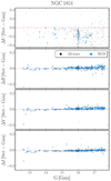 |
Fig. 2. Gaia synthetic photometry. Comparison between Gaia synthetic photometry generated from XP spectra and the photometry from Stetson et al. (2019) in the UBVI photometric bands, from top to bottom, respectively, for NGC 1851. Gray shaded points indicate all common stars in the two catalogs, while azure dots represent RGB cluster members in NGC 1851. |
The comparison reveals that synthetic BVI magnitudes are consistent with Stetson photometry, with differences less than 0.05 mag for stars brighter than G = 17, possibly due to small variations in the photometric zero point. However, synthetic U photometry displays larger and more variable differences with respect to Stetson U magnitudes, likely because the U filter is positioned at the blue edge of Gaia XP spectra, making the conversion process less reliable. Indeed, the top panel of Fig. 2 reveals a larger and random scatter with respect to that observed in the BVI filters7. We therefore only considered stars with a signal-to-noise ratio (S/N) greater than 30 when dealing with U magnitudes, following the guidelines of Gaia Collaboration (2023a). Nevertheless, the discrepancies in U magnitudes in NGC 1851 are not correlated with magnitude, position, or distance from the cluster center, making it impossible to use this photometric band to build the CUBI index. However, as NGC 1851 exhibits variations in heavy elements, we can make use of the Gaia-generated BVI magnitudes to study the properties of canonical and anomalous stars. In fact, as shown by Marino et al. (2015, see e.g., their Fig. 13), the pseudo-color CBVI = (B − V)−(V − I) index is an effective tool for identifying anomalous stars in type II GCs and investigating their properties. Furthermore, we calculated the photometric uncertainties in each band using the S/N provided by the GaiaXPy python library. By focusing on the sample of RGB stars, we determined the average photometric uncertainties to be 0.06, 0.03, and 0.02, with dispersions of 0.02, 0.01, and 0.009, respectively, for the B, V, I photometric filters.
3. Multiple populations along the color-magnitude diagrams
To identify multiple stellar populations with different heavy element content in NGC 1851, we employed the methodology outlined in previous studies (Marino et al. 2015; Milone et al. 2017; Cordoni et al. 2020b). In brief, this technique involves analyzing the I versus CBVI and I versus B − I CMDs, along with the resulting pseudo two-color diagram known as the chromosome map (ChM, Milone et al. 2017; Jang et al. 2022). Figure 3 provides a visual representation of this process.
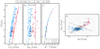 |
Fig. 3. Multiple stellar populations along the CMD. Panel a: I vs. CBVI pseudo-color diagram of NGC 1851 cluster members. Canonical and anomalous stars, selected in the Chm displayed in panel d, are respectively marked with filled azure and red dots. Empty diamonds indicate halo stars, i.e. stars outside the 11.7 arcmin tidal radius. Azure and red empty circles indicate metal-poor and metal-rich stars identified in Tautvaišienė et al. (2022), respectively. Average photometric uncertainties are shown as gray errorbars in panels a–c. Panel b: verticalized I vs. ΔBVI pseudo-color diagram color-coded as in panel a. Panel c: I vs. B − I CMD. Panel d: ΔBVI vs. ΔBI ChM. Stars are color-coded as in panel a. The gray line represents the line used to separate canonical and anomalous stars. Gray contours in the background represent the star density distribution as determined by means of 2D Gaussian KDE with fixed bandwidth. In the whole field of view, we identified 108 and 39 candidate canonical and anomalous stars, respectively, while outside the tidal radius we found eight and two canonical and anomalous stars, respectively. |
First, we determined the RGB boundaries in the as the 4th and 96th percentiles of the CBVI and B − I distribution using the approach from Milone et al. (2017). The color of each star was then converted into the verticalized color, denoted as  , where c, cR, and cB are the CBVI values for the stars and the blue and red fiducial lines, respectively. As a result, stars lying on the blue-red fiducial line have a ΔC = 0 and 1, respectively. The resulting verticalized colors are shown in Fig. 3b. Finally, we normalized each distribution to the color-width of the CMD at a I magnitude of 15. The normalized ΔC are displayed in the ChM in Fig. 3d. Average photometric uncertainties are displayed in Figs. 3a–c) with gray errorbars.
Clearly, the comparison of ΔBVI versus ΔBI ChM allows us to distinguish between the canonical and anomalous populations, which are manifested as two distinct clumps. Specifically, considering the average photometric uncertainties and the color distribution in the CBVI index, we restricted our analysis to stars brighter than I = 16, for which the separation between canonical and anomalous stars is more evident. To separate the two populations, we employed a combination of visual inspection and 2D Gaussian kernel density estimates (KDE), shown as gray-shaded contours in the background of Fig. 3d. The resulting classification is also displayed in Fig. 3d, where azure and red points correspond to canonical and anomalous stars, respectively, while the gray line indicates the adopted separation.
Our analysis suggests that 108 stars are likely canonical, while the remaining 39 are more consistent with being anomalous stars. Based on this classification, the population ratio of canonical stars with respect to the total number of stars is NCan/NTot = 0.735 ± 0.036. Specifically, 100 and 37 canonical and anomalous stars lie within the tidal radius yielding a ratio NCan/NTot = 0.730 ± 0.038, consistent with previous HST studies (see, e.g., Milone et al. 2017). On the other hand, eight and two stars, marked with large empty azure and red diamonds in Fig. 3, are consistent with being extra-tidal canonical and anomalous stars, respectively (NCan/NTot = 0.80 ± 0.10).
In order to demonstrate the effectiveness of the CBVI index in distinguishing between canonical and anomalous stars, we cross-matched our catalogs with stars with available spectroscopic information from Tautvaišienė et al. (2022). The empty large azure and red circles depicted in Fig. 3 correspond (respectively) to stars classified as metal-poor and metal-rich, as outlined in their Fig. 8 and Tables 1 and 2 of Tautvaišienė et al. (2022). Notably, the classification obtained using the CBVI index is in agreement with the findings of Tautvaišienė et al. (2022, see Sect. 3 for details), with only 3 out of 35 stars exhibiting inconsistencies.
Additionally, we show the BVI synthetic photometry generated for the residual field stars contaminants, identified as discussed in Sect. 2.1, as black crosses in Fig. 3. A visual inspection of Figs. 3a–d reveals that only two field stars exhibit pseudo-colors and magnitudes consistent with the bulk of NGC 1851 stars. Specifically, considering the ChM in Fig. 3d, one star overlaps with the location of the canonical population, and one with the anomalous one. Such result further confirms the soundness of our findings concerning the canonical and anomalous populations.
3.1. Defining an optimal filter to identify multiple populations in type II globular clusters
In the following, we try to exploit Gaia XP spectra to build ad-hoc photometry to reflect the chemical compositions of multiple stellar populations, each with a different heavy-element content. Specifically, we adopt the classification of Sect. 3 as a benchmark sample of canonical and anomalous stars. The detailed analysis of synthetic spectra carried out in Dondoglio et al. (in prep.) revealed that the effectiveness of the CBVI index is mostly due to differences in the spectra of canonical and anomalous stars in the spectral range covered by the B filters. Specifically, to reproduce the observations, anomalous stars must be enhanced in C+N+O. In particular, as found in Yong et al. (2015), N varies, while C and O remain constant. On this note, we perform an exploitative analysis on canonical and anomalous XP spectra to confirm the presence of distinctive features in the B spectral range.
To convert the set of BP − RP coefficients into a single externally calibrated spectrum, we used the GaiaXPy.calibrate function. The resulting spectrum is expressed in units of Wm−2 nm−1 and is dependent on the wavelength λ, measured in nanometers (nm). Figures 4b and c depict the calibrated spectra with relative flux uncertainties for two pairs of reference canonical and anomalous stars, marked with pentagons and triangles, respectively, in Fig. 4a.
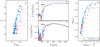 |
Fig. 4. Effectiveness of the f415 photometric filter. Panel a: I vs. CBVI CMD, as in Fig. 3a. Stars are colored azure and red according to the classification described in Sect. 3, i.e., canonical and anomalous. Gray errorbars represent the average photometric uncertainties determined in different magnitude bins. Panels b and c: externally calibrated Gaia XP spectra of two couples of reference canonical and anomalous stars, indicated with pentagons and triangles in panel a. The gray shaded rectangular regions indicate the f41525 filter, designed to identify canonical and anomalous stars. Fluxes are expresses in units of Wm−2 nm−1. Azure and red shaded regions indicate flux uncertainties. Panel d: mf41525 vs. mf41525 − I, where mf41525 is the magnitude computed by convolving externally calibrated spectra with the f41525 filter shown in panel a as in Eq. (5). Reference canonical and anomalous stars are enclosed by empty pentagons and triangles, while metal-poor and metal-rich stars from Tautvaišienė et al. (2022) are marked with empty circles. |
A qualitative examination of the spectra in Figs. 4b and c reveals that: (i) The fluxes in the UV region (λ ≲ 400 nm) exhibit significant fluctuations. (ii) Both sets of canonical and anomalous stars display notable flux differences in the spectral range between 400 and 430 nm. (iii) There are no discernible differences in the spectra for wavelengths λ ≳ 450 nm. For consistency, we checked that the same considerations are also true for different couples of canonical and anomalous stars selected randomly. Based on these findings, we have defined a box-shaped filter, denoted as f41525 and illustrated in Figs. 4b and c. The chosen name for the filter is based on indicating both its central wavelength and width. This filter, which encompasses the wavelength range between 405 and 430 nm, is characterized by a rectangular transmission curve with a 100% transmission efficiency across the specified wavelength range and zero outside of it.
To convolve the externally calibrated with the f415 filter, we used the following equation:
 (5)
(5)
where c is the speed of light in Å s−1, S is the stellar spectrum in erg s−1 cm−2 Å−1, F is the filter transmission curve, and λ represents the wavelength in units of Å. We then computed the magnitude as:

In Fig. 4d, we present mf415 versus mf415 − I CMD, where I represents the magnitude computed in the standardized JKC photometric systems, as discussed in Sect. 2.2. The canonical and anomalous stars selected in panel a are once again denoted by pentagons and triangles, respectively. Additionally, the metal-poor and metal-rich stars identified in Tautvaišienė et al. (2022) are indicated by empty large azure and red circles, respectively. Average photometric uncertainties, determined by means of the S/N, as discussed in Sect. 2.2, are shown in Figs. 4a–d as gray error bars.
The ad hoc designed f415 photometric filter effectively separates bright RGB stars into canonical and anomalous groups. The color separation between canonical and anomalous stars varies from 0.1 mag at the at the bottom of the RGB to nearly 0.4 mag for stars with mf41525 ∼ 16. To further demonstrate the effectiveness of the f415 filter, we show in Appendix A.1 the verticalized mf41525 versus mf41525 − I CMD and the verticalized color distribution in different magnitude bins. We refer to Appendix A.1 for a detailed description and analysis of the results.
3.2. Tentative identification of multiple populations with light-element variations
Moreover, the UV spectral region plays a crucial role in identifying MPs with variations in light-element abundances, as supported by the effectiveness of the Johnson U filter, as well as the HST F275W and F336W filters in separating 1P and 2P stars in Galactic GCs (Milone et al. 2012, 2017; Piotto et al. 2015).
Therefore, we attempted to define a second ad-hoc photometric filter encompassing the 350–390 nm wavelength range, dubbed f36025. As in the case of the f41525 filter, the name of the filter indicates both the central wavelength and the width of the filter. However, the low quality and large fluctuations of the spectra in the UV region hinders the accurate computation of synthetic magnitudes, thereby preventing us from utilizing this spectral region for investigating abundance by using photometry. The detailed analysis of the performance of the filter is carried out in Appendix A.2.
4. Properties and internal dynamics of multiple populations
In this section, we will analyze the morphology and the kinematics of the canonical and anomalous stellar populations identified in Sect. 2.2. In this context, the outer regions of the cluster are particularly important. In most formation scenarios, 2P stars form in the cluster center, leading to the formation of a more centrally concentrated new stellar generation. Consequently, first-population stars are expected to dominate the cluster’s outskirts.
In addition, theoretical and N-body dynamical simulations, have shown that the present-day morphology and internal dynamics of multiple populations are strongly influenced by the initial configuration of the stellar population. In other words, the dynamical evolution of multiple populations in single- and multi-generational scenarios may follow different paths. For example, in multi-generational scenarios, the anisotropy profile of first-population stars should differ significantly from that of second-population stars in the outermost regions of the cluster (Mastrobuono-Battisti & Perets 2013; Hénault-Brunet et al. 2015; Vesperini et al. 2018, 2021; Tiongco et al. 2019; Sollima 2021).
Recently, Cordoni et al. (2020a,b) used Gaia DR2 to investigate the kinematics of seven type I and two type II Galactic GCs and found evidence of different dynamics and morphologies in at least four of the analyzed clusters. Here, we adopt a similar approach to investigate the internal dynamics of canonical and anomalous stars in NGC 1851 up to a distance of approximately 45 arcmin from the cluster center.
4.1. Morphology of multiple populations
To analyze the spatial distribution of canonical and anomalous stars we fitted ellipses to the distribution of stars located within the tidal radius. Indeed, as the tidal tail of NGC 1851, mostly located in the southern quadrants (Kuzma et al. 2018), exhibit spatial asymmetry (see, e.g., Figs. 5a1–b1), we excluded extra-tidal stars from the fitting procedure and fitted canonical and anomalous cluster stars within the tidal radius with an ellipse to determine their ellipticity (ϵ = 1 − b/a), position angle (θ), and center. The uncertainties on the parameters were obtained by bootstrapping the results 1000 times. The best fit ellipses are shown in Figs. 5a2–b2 with solid thick azure-red lines, and the bootstrapped fits with shaded thin lines. The black solid lines represent the inferred position angles, and the shaded azure-red regions indicate their uncertainties.
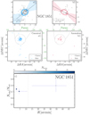 |
Fig. 5. Morphology of multiple stellar populations. Panels a1–b1: spatial distribution of canonical and anomalous stars, shown respectively in azure and red colors. Stars within the tidal radius are marked as filled dots, while extra-tidal stars are represented with crosses. The 11.7 arcmin tidal radius is indicated by the gray circles. Physical units, namely, parsecs, are displayed on the top and right axis in green. Panels a2–b2: zoom of the cluster field, with the best-fit ellipses shown as solid thick azure and red lines, and the position angle indicated by the solid black lines. Uncertainties are represented by the shaded regions. Panel c: radial distributions of canonical stars. The color is representative of the number of stars contained within each bin, while the gray dashed line indicates the tidal radius. |
Our results suggest that the canonical and anomalous populations possibly have different morphologies, with the anomalous population being more elliptical (with ϵ = 0.22 ± 0.10) than the canonical population (ϵ = 0.09 ± 0.07). However, the large relative uncertainties prevent us from drawing firm conclusions.
To investigate the radial distribution of multiple stellar populations in NGC 1851, namely, the ratio between canonical and anomalous stars as a function of radial distance from the cluster center, we divided the region between 1.5 arcmin and the tidal radius into two circular annuli, each containing approximately the same number of stars, while all the extra-tidal stars are included in a unique annulus. We calculated the ratio of canonical stars over the total number of stars for each bin. We performed this analysis using different numbers of bins to evaluate the impact of binning choice, and we found that the results were consistent.
Figure 5c displays the radial distribution of canonical stars in NGC 1851. Each point is color-coded according to the number of stars contained in the bin. A visual inspection of Fig. 5c indicates that, at odds with Zoccali et al. (2009), the population ratio is relatively constant within the tidal radius, but increases beyond it, reaching a value of NCan/NTot = 0.80 ± 0.10. Specifically, we detected eight canonical and two anomalous stars beyond the tidal radius of 11.7 arcmin. Therefore, it appears that the halo of NGC 1851 is dominated by stars belonging to the canonical populations, in agreement with the finding of Marino et al. (2014). Nonetheless, we recall that given the low number of stars, the outer halo ratio is consistent with the average population ratio, that is, 0.735 ± 0.036. We suggest that the discrepancy with the results of Zoccali et al. (2009) may be attributed to the asymmetric distribution of anomalous stars, which can introduce local gradients in the population ratio.
4.2. Internal dynamics of multiple stellar populations
As mentioned in the previous paragraphs, the present-day internal dynamics of MPs provides an important vantage point on the formation of multiple populations and in turn of GCs. On the same note, the clusters’ outskirts, which are characterized by longer relaxation times, are more likely to retain initial morphological and/or dynamical differences. In this work, we adopt a similar approach to previous Gaia-based studies (see, e.g., Vasiliev & Baumgardt 2021; Bianchini et al. 2018, 2019; Cordoni et al. 2020a,b) to investigate the internal dynamics of canonical and anomalous stars in NGC 1851. First, we convert the proper motions to sky-projected radial and tangential components, denoted as μRAD and μTAN, respectively, and propagate their uncertainties and covariance. Positive μRAD values indicate expansion, while positive μTAN values indicate counter-clockwise rotation. Next, we computed the radial and tangential dynamical profiles, that is, mean motion and velocity dispersion profiles, by minimizing the log-likelihood function presented in Bianchini et al. (2018), with an updated covariance term from Sollima et al. (2019), as in Bianchini et al. (2019). The mean radial motion has been corrected for the expected apparent contraction or expansion due to the cluster’s motion along the line of sight (see, e.g., Eqs. (2) and (3) of Bianchini et al. 2018). We divided the canonical and anomalous populations into four and three annular bins with equal number of stars, respectively, and minimized the likelihood using the Nelder-Mead method with the scipy minimizer (Virtanen et al. 2020). Additionally, we treat extra-tidal canonical stars in a separate bin, while due to the limited number of anomalous halo stars (two stars), we cannot analyze them separately. Finally, we calculate the anisotropy parameter as β = σTAN/σRAD − 1, where positive and negative values of β correspond to tangentially and radially anisotropic motion, respectively.
The uncertainties associated with the mean motion and velocity dispersion measurements were determined using the Markov chain Monte Carlo algorithm emcee (Foreman-Mackey et al. 2013). The mean motion and dispersion profiles are presented in Figs. 6 and 7, respectively, for the canonical and anomalous stellar populations with azure and red colors. The distance from the cluster center is expressed in arcmin and parsecs, respectively on the bottom and top axes. Dynamical profiles are instead represented in mas yr−1 and km s−1 on the left and right axes. The green color is used to indicate parsecs and km s−1, which have been converted adopting a distance of 11.95 kpc and a line-of-sight system velocity of 321.4 km s−1 (Baumgardt et al. 2019).
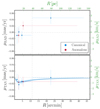 |
Fig. 6. Mean motion of multiple stellar populations. Mean motion along the radial (top panel) and tangential (bottom panel) direction. Azure and red points indicate canonical and anomalous dynamical profile. Physical units (i.e., parsec and km s−1) are displayed in the top and right axis in green. |
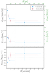 |
Fig. 7. Velocity dispersion profile of multiple stellar populations. Dispersion profile along the radial (top panel) and tangential (middle panel) direction. Azure and red points indicate canonical and anomalous dynamical profile. Physical units (i.e., parsec and km s−1) are displayed in the top and right axis in green. The anisotropy profile is shown in the bottom panel. |
Our analysis of NGC 1851 reveals that canonical and anomalous stars share similar average motion along both the radial and tangential directions. Specifically, in the innermost regions of the cluster, both the canonical and anomalous stellar populations exhibit negligible radial motion. However, as we move outwards, there is a noticeable increase in positive radial motion, suggesting that stars in this region have a tendency to move on highly radial orbits, potentially escaping from the cluster.
In contrast, the mean motion along the tangential direction displays a specific pattern. The central regions of NGC 1851 exhibit negative tangential motions, indicating a clockwise rotation. On the other hand, extra-tidal stars show no significant rotation. This rotational pattern aligns with the expected rotation curve of GCs, (see, e.g., Mackey et al. 2013; Kacharov et al. 2014; Bianchini et al. 2018),
 (6)
(6)
where the maximum rotational velocity is typically observed within a few arcminutes from the cluster center. The best-fit of the mean tangential motion of canonical stars is represented in Fig. 6 as a solid azure line, while the shaded region indicates the corresponding uncertainties.
The velocity dispersion profiles in Fig. 7 show a characteristic trend, decreasing as we move away from the cluster center in both the radial and tangential directions, which agrees with typical behavior observed in GCs. At the tidal radius, the dispersion reaches a value of around 0.04 mas yr−1 or 2 km s−1.
Notably, when examining the canonical population, the innermost regions (within 3 arcmin) display a larger radial velocity dispersion compared to the tangential dispersion, while extra-tidal stars show a slightly larger tangential velocity dispersion. Moreover, although the anomalous population exhibits a slightly larger tangential dispersion compared to canonical stars, the dispersion profiles of both populations are consistent within their uncertainties.
Additionally, it is noteworthy that the velocity dispersion in the outermost regions reaches a plateau. This behavior, characterized by an increasing or flat dispersion profile in cluster’s outskirts, deviates from the expected trend for LIMEPY/SPES models (Gieles & Zocchi 2015; de Boer et al. 2019; Claydon et al. 2019) and is similar to what is observed by Wan et al. (2023) in the GCs NGC 1261, NGC 1851, and NGC 1904. A plausible interpretation for this observed dispersion profile is the tidal interaction with the Galaxy. We mention here that, a qualitative comparison with Fig. 9 from Wan et al. (2023) reveals that we obtain a lower value of the velocity dispersion profile compared to theirs, for instance, 2 km s−1 against 5 km s−1. On the other hand, the small number of stars, that is, eight canonical stars, prevent us from drawing firm conclusions.
The anisotropy profile of canonical and anomalous stars is presented in the bottom panel of Fig. 7. In the case of the canonical population, the motion initially exhibits a radially anisotropic behavior in the innermost regions, at approximately 2–3 arcmin from the cluster center; meanwhile, as we move towards the cluster halo, the anisotropy possibly transitions to tangential. On the other hand, the anomalous population displays an isotropic motion at a distance of 3–4 arcmin from the cluster center and exhibits hints of tangential anisotropy in the outer regions.
These findings suggest that the stellar populations of NGC 1851 follow a typical behavior observed in other GCs (e.g., Bellini et al. 2015; Milone et al. 2018; Cordoni et al. 2020a). Similar conclusions were drawn by Libralato et al. (2023), who analyzed the proper motions of 1P, 2P, and anomalous stars in the inner ∼2.7 × 2.7 arcmin regions of 56 GCs and concluded that, when combining together the results from all dynamically old clusters i.e. Age/trh > 108, 2P stars exhibit isotropic motions at the cluster center but become radially anisotropic at approximately half-light radius. On the other hand, 1P and anomalous stars are consistent with being isotropic across their observed field of view (see, e.g., the top-row panels in Fig. 3 of Libralato et al. 2023).
To evaluate the impact of binning on the results, the dynamical profiles of the canonical stars were recomputed for different number of bins. Consistent results were obtained across different binning choices. Overall, the mean motions of the canonical and anomalous stars are similar, with hints of possible differences concerning the tangential dispersion profiles.
In Fig. 8, we present a comparison of our 1D velocity dispersion profiles with previous literature studies. Additionally, we show the overall 1D dispersion profile, computed for all stars, regardless of their canonical and anomalous identification, as gray markers in Fig. 8. Such profiles can be directly compared with the profile obtained by Vasiliev & Baumgardt (2021), denoted by the green line. Moreover, Fig. 8 also shows the dispersion profile of canonical and anomalous stars determined in Marino et al. (2014) from line-of-sight velocities, and the overall dispersion profile of Baumgardt et al. (2019), obtained combining Gaia DR2 proper motions with line-of-sight velocities. A visual examination of Fig. 8 suggests a good overall agreement between our 1D velocity dispersion profiles and those reported in the literature.
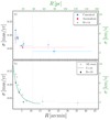 |
Fig. 8. Comparison with literature 1D velocity dispersion profiles. Panel a: comparison with literature velocity dispersion profiles, determined from line-of-sight velocity measurements, of canonical and anomalous stars from Marino et al. (2014), respectively shown with azure and red empty triangles. Extra-tidal stars dispersion in indicated by the purple empty triangle. Panel b: 1D velocity dispersion profile from proper motions from Baumgardt et al. (2019), Vasiliev & Baumgardt (2021), represented by the black diamonds and green line, respectively. Dynamical profiles have been determined from all cluster stars. Grey circles indicate the 1D velocity dispersion computed in this work analyzing all cluster stars, regardless of their canonical or anomalous classification. |
5. Summary and conclusions
We investigated the morphological and dynamical properties of multiple populations in NGC 1851 by using Gaia DR3 (Gaia Collaboration 2023b). To accomplish this, we made use the python package GaiaXPy to convert Gaia DR3 low-resolution XP spectra into synthetic photometry in the JKC standardized photometric system (Montegriffo et al. 2023; Gaia Collaboration 2023a) and generating UBVI photometry.
Specifically, we derived the CBVI = (B − V)−(V − I) index, which is a powerful tool to identify stellar populations with different metallicities among the bright RGB stars of GCs (Marino et al. 2015). Moreover, we define a new photometric filter, here dubbed f415, which isolates a distinctive feature of canonical and anomalous stars, located approximately at 400 nm and maximizes the separation between the canonical and anomalous stars (i.e., s-poor and s-rich stars). The main results on the morphology of multiple populations and on their radial and spatial distributions include:
-
The overall fraction of canonical stars contained within the tidal radius is 0.730 ± 0.038 and is consistent with results from previous studies (e.g., Milone et al. 2009).
-
We confirm the presence of an halo of cluster members that surrounds NGC 1851 and extends beyond the tidal radius up to more than 45 arcmin. The halo is predominantly composed of canonical stars, which comprise the 80 ± 10% of the total number of stars. This finding is in line with the conclusions of Marino et al. (2014), who, based on an analysis of spectra from the Very Large Telescope for seven extra-tidal stars, also reported that the NGC 1851 halo is primarily composed of the canonical population.
-
The canonical and anomalous population exhibit a flat radial distribution in the entire field of view, in agreement with Milone et al. (2009). While the canonical population has a nearly circular distribution, the anomalous stars show elliptical shapes.
We analyzed the proper motions of the canonical and anomalous populations over the entire field of view. In particular, we expand the analysis of the kinematics of multiple stellar populations beyond the tidal radius for the first time. This is crucial information for understanding the origin of GCs and their multiple stellar populations. Indeed, while dynamical differences in the inner regions may be erased by relaxation processes, the outskirts of the cluster, characterized by longer relaxation timescales, are more likely to retain evidence of distinct dynamical evolution. Our findings can be summarized as follows:
-
Canonical and anomalous stars exhibit similar mean motions in the radial and tangential directions. Specifically, both populations display positive radial motions in the outskirts, indicating a tendency for stars to escape the cluster on radial orbits. The tangential velocity profile, which serves as a proxy for on-sky rotation, shows a peak at approximately 3 arcmin (i.e., ∼10 parsec), followed by a decline to zero outside the tidal radius. Such pattern is consistent with the expected rotation of GCs.
-
The canonical population appears to have a slightly lower tangential velocity dispersion compared to the anomalous population, while no significant differences are observed in the radial velocity dispersion profile.
-
The velocity dispersion profiles exhibit a flat/increasing trend in the outskirt regions. This results, which is similar to findings of Wan et al. (2023) for the GCs NGC 1261, NGC 1851, and NGC 1904, is in disagreement with the expectations from LIMEPY/SPES models (Gieles & Zocchi 2015; de Boer et al. 2019; Claydon et al. 2019).
-
In the outskirts of the cluster, both canonical and anomalous populations display some hints of tangentially anisotropic motion. In contrast, in the innermost regions, the canonical population shows radial anisotropy, while anomalous stars exhibit isotropic motion.
In general, our study demonstrates that Gaia DR3 low-resolution XP spectra, together with Gaia DR3 astrometry and proper motions, are powerful tools to investigate multiple populations in GCs. We provided a comprehensive analysis of the canonical and anomalous populations in the type II GC NGC 1851 and its halo. The distinct behaviors in the morphology and in the internal dynamics of canonical and anomalous stars, have been followed in different regions of the cluster. These findings enhance our understanding of the dynamical processes and evolution of multiple stellar populations within globular clusters.
In this study, we will adopt the terminology introduced by Milone et al. (2017), where type I GCs are characterized by the presence of typical multiple populations with variations in light-element abundances. On the other hand, clusters that exhibit variations in both light- and heavy-elements are classified as type II GCs.
Various photometric diagrams constructed with ultraviolet filters, such as the B vs. U − B, B vs. U − B + I, and B vs. U − 2B + 1, are efficient tools to identify stellar populations with different light-element abundance in GCs (e.g., Marino et al. 2008; Milone et al. 2012; Jang et al. 2022). However, we verified that the U-band photometry derived from Gaia DR3 XP spectra of NGC 1851 is not accurate enough to disentangle 1P and 2P stars.
Even though there is little agreement on the exact value of the NGC 1851 tidal radius, (see, e.g., McLaughlin & van der Marel 2005; Harris 1996, revision of 2010), here, we opt for the largest value.
The code to use such routine is publicly available on GitHub https://github.com/GalacticDynamics-Oxford/GaiaTools
We note that the y-axis range in the top panel of Fig. 2 is almost twice as large as that displayed in all the three lower panels.
In the case of NGC 1851 Age/trh ∼ 14.
Acknowledgments
We thank the anonymous referee for his/her comments which improved the quality of the manuscript. A.F.M., G.C., and A.P.M. acknowledge the support received from INAF Research GTO-Grant Normal RSN2-1.05.12.05.10 – Understanding the formation of globular clusters with their multiple stellar generations (ref. Anna F. Marino) of the “Bando INAF per il Finanziamento della Ricerca Fondamentale 2022”. This work has received funding from the European Union’s Horizon 2020 research and innovation programme under the MarieSklodowska-Curie Grant Agreement No. 101034319 and from the European Union – NextGenerationEU, beneficiary: Ziliotto. This work has made use of data from the European Space Agency (ESA) mission Gaia (https://www.cosmos.esa.int/gaia), processed by the Gaia Data Processing and Analysis Consortium (DPAC, https://www.cosmos.esa.int/web/gaia/dpac/consortium). Funding for the DPAC has been provided by national institutions, in particular the institutions participating in the Gaia Multilateral Agreement. This job has made use of the Python package GaiaXPy, developed and maintained by members of the Gaia Data Processing and Analysis Consortium (DPAC), and in particular, Coordination Unit 5 (CU5), and the Data Processing Centre located at the Institute of Astronomy, Cambridge, UK (DPCI). S.J. acknowledges support from the NRF of Korea (2022R1A2C3002992, 2022R1A6A1A03053472). The data underlying this article will be shared on reasonable request to the corresponding author.
References
- Bastian, N., & Lardo, C. 2018, ARA&A, 56, 83 [Google Scholar]
- Bastian, N., Lamers, H. J. G. L. M., de Mink, S. E., et al. 2013, MNRAS, 436, 2398 [CrossRef] [Google Scholar]
- Baumgardt, H., Hilker, M., Sollima, A., & Bellini, A. 2019, MNRAS, 482, 5138 [Google Scholar]
- Bekki, K., & Yong, D. 2012, MNRAS, 419, 2063 [NASA ADS] [CrossRef] [Google Scholar]
- Bellini, A., Vesperini, E., Piotto, G., et al. 2015, ApJ, 810, L13 [NASA ADS] [CrossRef] [Google Scholar]
- Bianchini, P., van der Marel, R. P., del Pino, A., et al. 2018, MNRAS, 481, 2125 [Google Scholar]
- Bianchini, P., Ibata, R., & Famaey, B. 2019, ApJ, 887, L12 [NASA ADS] [CrossRef] [Google Scholar]
- Carballo-Bello, J. A., Martínez-Delgado, D., Navarrete, C., et al. 2018, MNRAS, 474, 683 [Google Scholar]
- Carretta, E., Gratton, R. G., Lucatello, S., et al. 2010, ApJ, 722, L1 [NASA ADS] [CrossRef] [Google Scholar]
- Cassisi, S., Salaris, M., Pietrinferni, A., et al. 2008, ApJ, 672, L115 [NASA ADS] [CrossRef] [Google Scholar]
- Claydon, I., Gieles, M., Varri, A. L., Heggie, D. C., & Zocchi, A. 2019, MNRAS, 487, 147 [NASA ADS] [CrossRef] [Google Scholar]
- Cordoni, G., Milone, A. P., Marino, A. F., et al. 2020a, ApJ, 898, 147 [NASA ADS] [CrossRef] [Google Scholar]
- Cordoni, G., Milone, A. P., Mastrobuono-Battisti, A., et al. 2020b, ApJ, 889, 18 [Google Scholar]
- Cordoni, G., Milone, A. P., Marino, A. F., et al. 2023, A&A, 672, A29 [NASA ADS] [CrossRef] [EDP Sciences] [Google Scholar]
- De Angeli, F., Weiler, M., Montegriffo, P., et al. 2023, A&A, 674, A2 [NASA ADS] [CrossRef] [EDP Sciences] [Google Scholar]
- de Boer, T. J. L., Gieles, M., Balbinot, E., et al. 2019, MNRAS, 485, 4906 [Google Scholar]
- Decressin, T., Meynet, G., Charbonnel, C., Prantzos, N., & Ekström, S. 2007, A&A, 464, 1029 [NASA ADS] [CrossRef] [EDP Sciences] [Google Scholar]
- Denissenkov, P. A., & Hartwick, F. D. A. 2014, MNRAS, 437, L21 [Google Scholar]
- D’Ercole, A., D’Antona, F., Ventura, P., Vesperini, E., & McMillan, S. L. W. 2010, MNRAS, 407, 854 [Google Scholar]
- Foreman-Mackey, D., Hogg, D. W., Lang, D., & Goodman, J. 2013, PASP, 125, 306 [Google Scholar]
- Gaia Collaboration (Montegriffo, P., et al.) 2023a, A&A, 674, A33 [CrossRef] [EDP Sciences] [Google Scholar]
- Gaia Collaboration (Vallenari, A., et al.) 2023b, A&A, 674, A1 [NASA ADS] [CrossRef] [EDP Sciences] [Google Scholar]
- Gieles, M., & Zocchi, A. 2015, MNRAS, 454, 576 [NASA ADS] [CrossRef] [Google Scholar]
- Gieles, M., Charbonnel, C., Krause, M. G. H., et al. 2018, MNRAS, 478, 2461 [Google Scholar]
- Harris, W. E. 1996, AJ, 112, 1487 [Google Scholar]
- Helmi, A., Babusiaux, C., Koppelman, H. H., et al. 2018, Nature, 563, 85 [Google Scholar]
- Hénault-Brunet, V., Gieles, M., Agertz, O., & Read, J. I. 2015, MNRAS, 450, 1164 [CrossRef] [Google Scholar]
- Jang, S., Milone, A. P., Legnardi, M. V., et al. 2022, MNRAS, 517, 5687 [CrossRef] [Google Scholar]
- Kacharov, N., Bianchini, P., Koch, A., et al. 2014, A&A, 567, A69 [NASA ADS] [CrossRef] [EDP Sciences] [Google Scholar]
- Kuzma, P. B., Da Costa, G. S., & Mackey, A. D. 2018, MNRAS, 473, 2881 [Google Scholar]
- Lardo, C., Milone, A. P., Marino, A. F., et al. 2012, A&A, 541, A141 [NASA ADS] [CrossRef] [EDP Sciences] [Google Scholar]
- Libralato, M., Vesperini, E., Bellini, A., et al. 2023, ApJ, 944, 58 [CrossRef] [Google Scholar]
- Lindegren, L., Hernández, J., Bombrun, A., et al. 2018, A&A, 616, A2 [NASA ADS] [CrossRef] [EDP Sciences] [Google Scholar]
- Mackey, A. D., Da Costa, G. S., Ferguson, A. M. N., & Yong, D. 2013, ApJ, 762, 65 [CrossRef] [Google Scholar]
- Marino, A. F., Villanova, S., Piotto, G., et al. 2008, A&A, 490, 625 [NASA ADS] [CrossRef] [EDP Sciences] [Google Scholar]
- Marino, A. F., Milone, A. P., Yong, D., et al. 2014, MNRAS, 442, 3044 [NASA ADS] [CrossRef] [Google Scholar]
- Marino, A. F., Milone, A. P., Karakas, A. I., et al. 2015, MNRAS, 450, 815 [NASA ADS] [CrossRef] [Google Scholar]
- Marino, A. F., Milone, A. P., Renzini, A., et al. 2019, MNRAS, 487, 3815 [CrossRef] [Google Scholar]
- Mastrobuono-Battisti, A., & Perets, H. B. 2013, ApJ, 779, 85 [NASA ADS] [CrossRef] [Google Scholar]
- McLaughlin, D. E., & van der Marel, R. P. 2005, ApJS, 161, 304 [NASA ADS] [CrossRef] [Google Scholar]
- Milone, A. P., & Marino, A. F. 2022, Universe, 8, 359 [NASA ADS] [CrossRef] [Google Scholar]
- Milone, A. P., Bedin, L. R., Piotto, G., et al. 2008, ApJ, 673, 241 [NASA ADS] [CrossRef] [Google Scholar]
- Milone, A. P., Stetson, P. B., Piotto, G., et al. 2009, A&A, 503, 755 [NASA ADS] [CrossRef] [EDP Sciences] [Google Scholar]
- Milone, A. P., Piotto, G., Bedin, L. R., et al. 2012, ApJ, 744, 58 [NASA ADS] [CrossRef] [Google Scholar]
- Milone, A. P., Piotto, G., Renzini, A., et al. 2017, MNRAS, 464, 3636 [Google Scholar]
- Milone, A. P., Marino, A. F., Mastrobuono-Battisti, A., & Lagioia, E. P. 2018, MNRAS, 479, 5005 [NASA ADS] [CrossRef] [Google Scholar]
- Milone, A. P., Marino, A. F., Da Costa, G. S., et al. 2020, MNRAS, 491, 515 [NASA ADS] [CrossRef] [Google Scholar]
- Montegriffo, P., De Angeli, F., Andrae, R., et al. 2023, A&A, 674, A3 [NASA ADS] [CrossRef] [EDP Sciences] [Google Scholar]
- Olszewski, E. W., Saha, A., Knezek, P., et al. 2009, AJ, 138, 1570 [NASA ADS] [CrossRef] [Google Scholar]
- Piotto, G., Milone, A. P., Bedin, L. R., et al. 2015, AJ, 149, 91 [Google Scholar]
- Renzini, A., Marino, A. F., & Milone, A. P. 2022, MNRAS, 513, 2111 [NASA ADS] [CrossRef] [Google Scholar]
- Riello, M., De Angeli, F., Evans, D. W., et al. 2018, A&A, 616, A3 [NASA ADS] [CrossRef] [EDP Sciences] [Google Scholar]
- Riello, M., De Angeli, F., Evans, D. W., et al. 2021, A&A, 649, A3 [NASA ADS] [CrossRef] [EDP Sciences] [Google Scholar]
- Shipp, N., Drlica-Wagner, A., Balbinot, E., et al. 2018, ApJ, 862, 114 [Google Scholar]
- Simpson, J. D., Martell, S. L., & Navin, C. A. 2017, MNRAS, 465, 1123 [NASA ADS] [CrossRef] [Google Scholar]
- Sollima, A. 2021, MNRAS, 502, 1974 [NASA ADS] [CrossRef] [Google Scholar]
- Sollima, A., Gratton, R. G., Carballo-Bello, J. A., et al. 2012, MNRAS, 426, 1137 [NASA ADS] [CrossRef] [Google Scholar]
- Sollima, A., Baumgardt, H., & Hilker, M. 2019, MNRAS, 485, 1460 [Google Scholar]
- Stetson, P. B., Pancino, E., Zocchi, A., Sanna, N., & Monelli, M. 2019, MNRAS, 485, 3042 [Google Scholar]
- Tautvaišienė, G., Drazdauskas, A., Bragaglia, A., et al. 2022, A&A, 658, A80 [CrossRef] [EDP Sciences] [Google Scholar]
- Tiongco, M. A., Vesperini, E., & Varri, A. L. 2019, MNRAS, 487, 5535 [NASA ADS] [CrossRef] [Google Scholar]
- Vasiliev, E., & Baumgardt, H. 2021, MNRAS, 505, 5978 [NASA ADS] [CrossRef] [Google Scholar]
- Ventura, P., Caloi, V., D’Antona, F., et al. 2009, MNRAS, 399, 934 [CrossRef] [Google Scholar]
- Vesperini, E., Hong, J., Webb, J. J., D’Antona, F., & D’Ercole, A. 2018, MNRAS, 476, 2731 [NASA ADS] [CrossRef] [Google Scholar]
- Vesperini, E., Hong, J., Giersz, M., & Hypki, A. 2021, MNRAS, 502, 4290 [NASA ADS] [CrossRef] [Google Scholar]
- Virtanen, P., Gommers, R., Oliphant, T. E., et al. 2020, Nat. Methods, 17, 261 [Google Scholar]
- Wan, Z., Arnold, A. D., Oliver, W. H., et al. 2023, MNRAS, 519, 192 [Google Scholar]
- Weiler, M., Carrasco, J. M., Fabricius, C., & Jordi, C. 2023, A&A, 671, A52 [NASA ADS] [CrossRef] [EDP Sciences] [Google Scholar]
- Yong, D., Grundahl, F., D’Antona, F., et al. 2009, ApJ, 695, L62 [NASA ADS] [CrossRef] [Google Scholar]
- Yong, D., Grundahl, F., & Norris, J. E. 2015, MNRAS, 446, 3319 [NASA ADS] [CrossRef] [Google Scholar]
- Zoccali, M., Pancino, E., Catelan, M., et al. 2009, ApJ, 697, L22 [NASA ADS] [CrossRef] [Google Scholar]
Appendix A: Performance of the f36025 and f41525 ad-hoc photometric filters
In the following, we review in greater detail the performance and effectiveness of the two newly defined photometric filters, namely, f36025 and f41525. We remind here that, while the first is defined to reflect variations in light element abundances, namely, to separate 1P from 2P stars, the latter aims at effectively distinguishing canonical and anomalous stars, namely, stars with different heavy-element content.
A.1. Effectiveness of the f41525 photometric filter
Figure A.1 presents a more detailed analysis of the effectiveness of the f41525 filter in distinguishing between canonical and anomalous stars, i.e. stars with different heavy-element content. To evaluate the performance of the f41525 filter, we adopt the same approach used for identifying MPs in the I versus CBVI pseudo-CMD, shown in Fig.3. Specifically, we define the blue and red RGB boundaries as the 4th and 96th percentiles of the mf41525 − I distribution (Fig.A.1a), and calculate the verticalized Δ(mf41525 − I) (Fig. A.1b), as discussed in Sec.3. Finally, we analyze the distribution of the verticalized color in three different magnitude bins indicated by the gray horizontal lines in Fig. A.1b.
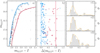 |
Fig. A.1. Effectiveness of the f41525 photometric filter. Panel a)mf41525 vs. mf41525 − I CMD. Canonical and anomalous stars, selected by means of the BVI index, are colored azure and red respectively. The azure and red fiducial lines mark the RGB boundaries, defined as the 4th and 96th percentile of the pseudo-color distribution. Average color and magnitude uncertainties are shown with the gray errorbars on the right of the CMD. Stars in common with Tautvaišienė et al. (2022) are marked with empty large circles. Panel b) Verticalized CMD of panel a). Panels c1-c3) Verticalized color distribution of stars in the three different magnitude ranges highlighted in panel b. The orange lines represent the Gaussian KDE. |
Fig. A.1 (c1-c3) illustrates the distribution of the verticalized Δ(mf41525 − I) color in the three magnitude bins. Remarkably, the Δ(mf41525 − I) distribution exhibits well separated peaks in all three magnitude bins, with the faintest bin displaying a certain degree of overlap. This figure suggests that the synthetic magnitude in the f41525 filter offers a clear identification of canonical and anomalous stars among bright RGB stars. However, for fainter RGB stars, the combination of increasing photometric uncertainties (as shown by the gray error bars in Fig.A.1a), larger flux fluctuations, and a narrower CMD diminishes the clarity of separation, resulting in some overlap between canonical and anomalous stars. Furthermore, the less pronounced separation among faint-RGB stars is partly attributed to the intrinsic nature of canonical and anomalous stars. Firstly, the distribution of C + N + O is continuous rather than discrete (see, e.g., Yong et al. 2015; Tautvaišienė et al. 2022), contributing to the reduced differentiation. Secondly, the separation also depends on stellar temperature, resulting in decreased distinction for colder faint-RGB stars. Similarly, this effect is evident in the CBVI index, which more effectively identifies canonical and anomalous stars among bright RGB stars.
Despite these limitations, the newly defined f41525 filter successfully identifies canonical and anomalous stars. This effectiveness establishes a strong foundation for its future utilization in forthcoming data releases.
A.2. Performance of the f36025 photometric filter
Similar to the f41525 filter, the f36025 filter is defined as a box-filter encompassing the 350-375 nm wavelength range. Such filter is defined as to include the absorption feature located approximately between 350-390 nm (see, e.g., panels b1-b2 of Fig. 4 in Milone et al. 2017) and to separate the bulk of 1P and 2P stars in NGC 1851. The comparison of I versus mf36025 − I CMD, depicted in Fig. A.2a, suggests that the RGB-spread is larger than what is expected from observational uncertainties alone, even though the sequences are not distinctly separated enough to provide a reliable identification. Nevertheless, a noticeable difference is observed in the RGB sequence of canonical and anomalous stars. Specifically, the RGB sequence of canonical stars spans a broader color range, whereas anomalous stars are predominantly located on a narrow sequence towards the red side of the RGB. This distinction becomes more prominent when considering stars brighter than I = 14, as they exhibit lower photometric uncertainties (indicated by gray error bars in Fig. A.2). A plausible explanation for this behavior is that canonical stars display a wider range of light element variations, in particular Nitrogen, compared to the anomalous stars (see, e.g., Lardo et al. 2012; Yong et al. 2015; Tautvaišienė et al. 2022). Similar considerations are also true for Fig. A.2b, even though the photometric index is affected by slightly larger uncertainties.
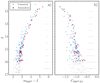 |
Fig. A.2. Performance of the f36025 photometric filter. Panel a)I vs. mf36025 − I CMD. Azure and red markers indicate canonical and anomalous stars, while photometric uncertainties are shown with gray errorbars. Panel b)I versus Cf36025, B, I = (mf36025 − B)−(B − I) CMD. Color-coding is the same as in panel a). |
Therefore, even though the f36025 filter yields promising results showing some indications of separation between 1P and 2P stars, it cannot be solely relied upon for unequivocal identification of first- and second-population stars in NGC 1851. Nevertheless, as Gaia XP spectra continue to improve in future data releases, the f36025 filter may become a valuable tool for extracting essential information about multiple stellar populations at the clusters’ outskirts.
All Figures
|
Fig. 1. Cluster members selection. Panel a: proper motion distance (μR) relative to NGC 1851 mean motion derived in Vasiliev & Baumgardt (2021), as a function of Gaia G magnitude. Cluster members are displayed as black shaded points, while residual field stars contaminants are shown with orange crosses. Panel b: parallax (ω) as a function of G magnitude. Panel c: uncertainty in proper motions (ϵμ) vs. Gaia G magnitude. Panel d: Δ RA vs. Δ Dec of the selected cluster members. Panel e: G vs. GBP − GRP CMD of the selected cluster members. |
| In the text | |
|
Fig. 2. Gaia synthetic photometry. Comparison between Gaia synthetic photometry generated from XP spectra and the photometry from Stetson et al. (2019) in the UBVI photometric bands, from top to bottom, respectively, for NGC 1851. Gray shaded points indicate all common stars in the two catalogs, while azure dots represent RGB cluster members in NGC 1851. |
| In the text | |
|
Fig. 3. Multiple stellar populations along the CMD. Panel a: I vs. CBVI pseudo-color diagram of NGC 1851 cluster members. Canonical and anomalous stars, selected in the Chm displayed in panel d, are respectively marked with filled azure and red dots. Empty diamonds indicate halo stars, i.e. stars outside the 11.7 arcmin tidal radius. Azure and red empty circles indicate metal-poor and metal-rich stars identified in Tautvaišienė et al. (2022), respectively. Average photometric uncertainties are shown as gray errorbars in panels a–c. Panel b: verticalized I vs. ΔBVI pseudo-color diagram color-coded as in panel a. Panel c: I vs. B − I CMD. Panel d: ΔBVI vs. ΔBI ChM. Stars are color-coded as in panel a. The gray line represents the line used to separate canonical and anomalous stars. Gray contours in the background represent the star density distribution as determined by means of 2D Gaussian KDE with fixed bandwidth. In the whole field of view, we identified 108 and 39 candidate canonical and anomalous stars, respectively, while outside the tidal radius we found eight and two canonical and anomalous stars, respectively. |
| In the text | |
|
Fig. 4. Effectiveness of the f415 photometric filter. Panel a: I vs. CBVI CMD, as in Fig. 3a. Stars are colored azure and red according to the classification described in Sect. 3, i.e., canonical and anomalous. Gray errorbars represent the average photometric uncertainties determined in different magnitude bins. Panels b and c: externally calibrated Gaia XP spectra of two couples of reference canonical and anomalous stars, indicated with pentagons and triangles in panel a. The gray shaded rectangular regions indicate the f41525 filter, designed to identify canonical and anomalous stars. Fluxes are expresses in units of Wm−2 nm−1. Azure and red shaded regions indicate flux uncertainties. Panel d: mf41525 vs. mf41525 − I, where mf41525 is the magnitude computed by convolving externally calibrated spectra with the f41525 filter shown in panel a as in Eq. (5). Reference canonical and anomalous stars are enclosed by empty pentagons and triangles, while metal-poor and metal-rich stars from Tautvaišienė et al. (2022) are marked with empty circles. |
| In the text | |
|
Fig. 5. Morphology of multiple stellar populations. Panels a1–b1: spatial distribution of canonical and anomalous stars, shown respectively in azure and red colors. Stars within the tidal radius are marked as filled dots, while extra-tidal stars are represented with crosses. The 11.7 arcmin tidal radius is indicated by the gray circles. Physical units, namely, parsecs, are displayed on the top and right axis in green. Panels a2–b2: zoom of the cluster field, with the best-fit ellipses shown as solid thick azure and red lines, and the position angle indicated by the solid black lines. Uncertainties are represented by the shaded regions. Panel c: radial distributions of canonical stars. The color is representative of the number of stars contained within each bin, while the gray dashed line indicates the tidal radius. |
| In the text | |
|
Fig. 6. Mean motion of multiple stellar populations. Mean motion along the radial (top panel) and tangential (bottom panel) direction. Azure and red points indicate canonical and anomalous dynamical profile. Physical units (i.e., parsec and km s−1) are displayed in the top and right axis in green. |
| In the text | |
|
Fig. 7. Velocity dispersion profile of multiple stellar populations. Dispersion profile along the radial (top panel) and tangential (middle panel) direction. Azure and red points indicate canonical and anomalous dynamical profile. Physical units (i.e., parsec and km s−1) are displayed in the top and right axis in green. The anisotropy profile is shown in the bottom panel. |
| In the text | |
|
Fig. 8. Comparison with literature 1D velocity dispersion profiles. Panel a: comparison with literature velocity dispersion profiles, determined from line-of-sight velocity measurements, of canonical and anomalous stars from Marino et al. (2014), respectively shown with azure and red empty triangles. Extra-tidal stars dispersion in indicated by the purple empty triangle. Panel b: 1D velocity dispersion profile from proper motions from Baumgardt et al. (2019), Vasiliev & Baumgardt (2021), represented by the black diamonds and green line, respectively. Dynamical profiles have been determined from all cluster stars. Grey circles indicate the 1D velocity dispersion computed in this work analyzing all cluster stars, regardless of their canonical or anomalous classification. |
| In the text | |
|
Fig. A.1. Effectiveness of the f41525 photometric filter. Panel a)mf41525 vs. mf41525 − I CMD. Canonical and anomalous stars, selected by means of the BVI index, are colored azure and red respectively. The azure and red fiducial lines mark the RGB boundaries, defined as the 4th and 96th percentile of the pseudo-color distribution. Average color and magnitude uncertainties are shown with the gray errorbars on the right of the CMD. Stars in common with Tautvaišienė et al. (2022) are marked with empty large circles. Panel b) Verticalized CMD of panel a). Panels c1-c3) Verticalized color distribution of stars in the three different magnitude ranges highlighted in panel b. The orange lines represent the Gaussian KDE. |
| In the text | |
|
Fig. A.2. Performance of the f36025 photometric filter. Panel a)I vs. mf36025 − I CMD. Azure and red markers indicate canonical and anomalous stars, while photometric uncertainties are shown with gray errorbars. Panel b)I versus Cf36025, B, I = (mf36025 − B)−(B − I) CMD. Color-coding is the same as in panel a). |
| In the text | |
Current usage metrics show cumulative count of Article Views (full-text article views including HTML views, PDF and ePub downloads, according to the available data) and Abstracts Views on Vision4Press platform.
Data correspond to usage on the plateform after 2015. The current usage metrics is available 48-96 hours after online publication and is updated daily on week days.
Initial download of the metrics may take a while.