| Issue |
A&A
Volume 699, July 2025
|
|
|---|---|---|
| Article Number | A41 | |
| Number of page(s) | 16 | |
| Section | Galactic structure, stellar clusters and populations | |
| DOI | https://doi.org/10.1051/0004-6361/202555214 | |
| Published online | 01 July 2025 | |
Neutron-capture element signatures in globular clusters
Insights from the Gaia-ESO Survey
1
INAF – Osservatorio Astrofisico di Arcetri,
Largo Enrico Fermi 5,
50125
Florence,
Italy
2
INAF – Osservatorio Astronomico di Padova,
Vicolo dell’Osservatorio 5,
35122
Padova,
Italy
3
INAF – Osservatorio di Astrofisica e Scienza dello Spazio di Bologna,
via P. Gobetti 93/3,
40129
Bologna,
Italy
4
Dipartimento di Fisica, Sezione di Astronomia, Università di Trieste,
Via G. B. Tiepolo 11,
34143
Trieste,
Italy
5
INAF – Osservatorio Astronomico di Trieste,
Via G.B. Tiepolo 11,
34143
Trieste,
Italy
6
INFN, Sezione di Trieste,
Via A. Valerio 2,
34127
Trieste,
Italy
7
Heidelberger Institut für Theoretische Studien,
Schloss-Wolfsbrunnenweg 35,
69118
Heidelberg,
Germany
8
Institute of Astronomy, University of Cambridge,
Madingley Road,
Cambridge
CB3 0HA,
UK
9
School of Physical and Chemical Sciences – Te Kura Matū, University of Canterbury,
Private Bag 4800,
Christchurch
8140,
New Zealand
10
ESO – European Southern Observatory,
Alonso de Cordova 3107, Vitacura,
Santiago,
Chile
11
Dipartimento di Fisica e Astronomia, Università degli Studi di Firenze,
Via Sansone 1,
50019
Sesto Fiorentino,
Italy
★ Corresponding author: This email address is being protected from spambots. You need JavaScript enabled to view it.
Received:
18
April
2025
Accepted:
12
May
2025
Abstract
Context. Globular clusters (GCs) are crucial to our understanding of the formation and evolution of our Galaxy. While their abundances of light and iron-peak elements have been extensively studied, research on heavier elements and their possible link to both the multiple stellar population phenomenon and the origin of GCs remains relatively limited.
Aims. We aim to analyse the chemical abundances of various neutron-capture elements using GCs as tracers of the Galactic halo. Furthermore, we explore the potential connection between these elements and the multiple stellar population phenomenon in GCs to better constrain the nature of the polluters responsible for the intracluster enrichment. Additionally, we seek to determine the origins of GCs based on their neutron-capture element abundances.
Methods. We analysed a sample of 14 GCs spanning a wide metallicity range, [Fe/H] from −0.40 to −2.32, observed as a part of the Gaia-ESO Survey and analysed using a homogeneous methodology. Here we present results for Y, Zr, Ba, La, Ce, Nd, Pr, and Eu obtained from FLAMES-UVES spectra. We compared our results with a stochastic Galactic chemical evolution model.
Results. Except for Zr, the Galactic chemical evolution model, when available, closely describes the broad trend displayed by neutron-capture elements in GCs. Moreover, in some clusters, a strong correlation between hot H-burning (Na and Al) and s-process elements suggests a shared nucleosynthetic site, for example asymptotic giant branch stars of different masses and/or fast-rotating massive stars that produced the intracluster pollution. Additionally, we identified clear differences in the [Eu/Mg] ratio between in situ (⟨[Eu/Mg]]⟩=0.14 dex) and ex situ (⟨[Eu/Mg]]⟩=0.32 dex GCs, which reveal their distinct chemical enrichment histories. Finally, on average, the Type II GCs NGC 362, NGC 1261, and NGC 1851 show a spread ratio in s-process elements between second- and first-generation stars that is roughly twice as large as that observed in Type I clusters.
Key words: Key words. stars: abundances / stars: Population II / globular clusters: general
© The Authors 2025
 Open Access article, published by EDP Sciences, under the terms of the Creative Commons Attribution License (https://creativecommons.org/licenses/by/4.0), which permits unrestricted use, distribution, and reproduction in any medium, provided the original work is properly cited.
This article is published in open access under the Subscribe to Open model. This email address is being protected from spambots. You need JavaScript enabled to view it. to support open access publication.
1 Introduction
Over the past few decades, globular clusters (GCs) have been the subject of extensive research. Their age and spatial distribution make them perfect candidates for studying the formation and evolution of the Galactic halo, disc, and bulge. With some exceptions (e.g. the GC E 3; Salinas & Strader 2015; Monaco et al. 2018), all the known Galactic GCs host multiple stellar populations (MPs), a phenomenon that is generally attributed to internal pollution caused by a subset of stars called ‘polluters’ (see e.g. Bastian & Lardo 2018; Gratton et al. 2019). While the first generation (FG) of stars displays a chemical pattern similar to that of field stars of the same metallicity, the second generation (SG) shows an altered composition in hot H-burning elements (specifically, a high content of N, Na, and Al but a depletion in C, O, and Mg). Although the presence of MPs in GCs is well established, it is still unclear what the sources with such altered compositions in SG stars are. Different mechanisms have been proposed, such as intermediate-mass (4–8 M⊙) asymptotic giant branch (AGB) stars (Ventura et al. 2001), fast-rotating massive stars (Meynet et al. 2006), massive binaries (de Mink et al. 2009), super-massive stars (Denissenkov et al. 2015), and non-canonical stellar evolution, including rotation and binarity (Pancino 2018). Although MPs have been extensively studied, most spectroscopic analyses have focused primarily on light and Fe-peak elements. So far, these observations have not been sufficient to determine the nature of the polluters. A more comprehensive chemical characterisation of other key elements, such as Li (see e.g. D’Orazi & Marino 2010; D’Orazi et al. 2014, 2015; Schiappacasse-Ulloa et al. 2022) and neutron-capture (n-capture) elements (see e.g. D’Orazi et al. 2010; Cohen 2011; Fernández-Trincado et al. 2021, 2022; Schiappacasse-Ulloa & Lucatello 2023), could provide deeper insights into the nature of the polluters.
The n-capture elements can be broadly classified into two categories based on their formation processes: rapid- (r-) and slow- (s-) process elements. The primary astrophysical sites of r-process nucleosynthesis remain a topic of debate. However, it is generally accepted that short-timescale sources, such as magneto-rotationally driven (MRD) supernovae (SNe; Nishimura et al. 2015) or collapsars (Siegel et al. 2019), contribute significantly to their production. Additionally, the merger of binary neutron star systems is expected to play a crucial role in r-process enrichment over longer timescales (see e.g. Perego et al. 2021; Cowan et al. 2021). On the other hand, the s-process happens in a variety of sources, including low-mass (1.2–4 M⊙) AGB stars (with some contribution from AGB stars of up to 8 M⊙) or rotating massive stars, which are efficiently producing first-peak s-process elements such as Y and Zr (Frischknecht et al. 2012; Limongi & Chieffi 2018) and, to some degree, second-peak s-process elements such as Ba, La, and Ce. Although the importance of these elements for identifying relevant nucleosynthetic sites is well recognised, only a limited number of studies on GCs have been conducted (see e.g. James et al. 2004). These studies have revealed a relatively homogeneous internal abundance of n-capture elements in the analysed GCs (see e.g. D’Orazi et al. 2010; Cohen 2011). Recently, Schiappacasse-Ulloa et al. (2024, hereafter SUL24) conducted a homogeneous analysis of Y, Ba, La, and Eu abundances in 18 GCs using Ultraviolet and Visual Echelle Spectrograph (UVES) spectra, the largest and most comprehensive sample analysed to date. Among their most remarkable results, they found evidence of a slight correlation between Y and Na in GCs with intermediate metallicities (−1.8<[Fe/H]<−1.1 dex), suggesting a potential modest production of light s-process elements alongside Na production.
Milone et al. (2017) classified GCs into two types based on their chemical properties. Type I GCs typically show uniform n-capture element abundances across their stellar populations despite minor iron variations. In contrast, Type II GCs exhibit more complex chemical patterns, often including significant spreads in iron and heavier elements such as those produced by the n-capture process. Similar to those observed in satellite galaxies, these chemical peculiarities could reflect their formation in distinct environments. Recently, efforts have been made to explore the potential chemical differences between GCs formed within our Galaxy (in situ GCs) and those born outside and later accreted (ex situ GCs). For example, Carretta & Bragaglia (2022) suggest that some of the GCs born in the Sagittarius dwarf galaxy could be distinguished by their Fe-peak abundance pattern, which displays lower Sc, V, and Zn than in situ stars. More recently, Monty et al. (2024) analysed a sample of 54 ex situ and in situ GCs, finding a clear difference in their [Eu/Si] ratio: accreted GCs exhibit elevated [Eu/Si] ratios, whereas in situ GCs show lower values.
In this regard, extensive spectroscopic surveys, such as the Gaia-ESO Survey (Gilmore et al. 2022; Randich et al. 2022), the Apache Point Observatory Galactic Evolution Experiment (APOGEE; Majewski et al. 2017), and the GALactic Archaeology with HERMES (GALAH; Buder et al. 2019), are significantly advancing our understanding of Galactic stellar populations and, in particular, of GCs. Gaia-ESO is the only large public survey to benefit from an 8 m class telescope and a spectrograph that achieves a resolving power R=47 000 (FLAMES equipped with UVES; Pasquini et al. 2002). These characteristics, along with the broad wavelength coverage (480.0-680.0 nm), the high signal-to-noise ratio (S/N), and homogeneous spectral analysis, enabled Gaia-ESO to perform a precise determination of a large number of element abundances simultaneously, including a large number of n-capture elements (see e.g. Magrini et al. 2018; Van der Swaelmen et al. 2023; Molero et al. 2023, 2025). Consequently, the Gaia-ESO data have the potential to enhance our understanding of the internal chemical enrichment of GCs while also providing valuable insights into their role in the formation and evolution of the Galaxy.
We built upon the analysis conducted by SUL24, expanding both the sample and the species analysed. We provide a homogeneous analysis of a large sample of GCs covering the full range of metallicities. We examined their internal spreads, explored their relationship with key elements in the context of the MP phenomenon, such as hot H-burning elements, and investigated any potential links to their origin.
In Sect. 2, we describe the selection of GC members. In Sect. 3, we detail the data reduction and abundance determination. Section 4 and Appendix A compare our results with the literature for in-common stars, and Appendix B describes trends in our results with the microturbulent velocity, Vt. In Sect. 5, we analyse the Gaia-ESO results in the Galactic context by using the predictions of an updated stochastic Galactic chemical evolution model. We study the n-capture relation and the MP indicators in Sect. 6 and Appendix C, and in Sect. 7 the internal spread of n-capture abundances in our sample GCs. In Sect. 8 we summarise our results.
2 Sample and membership selection
The Gaia-ESO Survey observed 14 GCs as calibrators of both stellar parameters and chemical abundances. The sample of GCs, together with the other stellar calibrators – open clusters, benchmark stars, asteroseismic targets – is described in Pancino et al. (2017a), while the results of their analysis, in the context of the global calibration and homogenisation of the survey, are reported in Hourihane et al. (2023). The GCs were selected to cover a wide metallicity range, extending from about [Fe/H] = −2.5 to −0.5. Their data have been used in various scientific studies, such as Lardo et al. (2015), Pancino et al. (2017b), and Tautvaišienė et al. (2022).
In our work, we accounted for the complete sample of GCs, using only the high-resolution UVES spectra with a signal-to-noise ratio larger than 501. To build our sample, we selected stars from the final Gaia-ESO release (Hourihane et al. 2023) that were observed with UVES and belonged to the GC fields. The latter condition corresponds to GES_TYPE = GE_SD_GC (for new Gaia-ESO observations) and AR_SD_GC (for archival data re-analysed in Gaia-ESO). This condition does not guarantee that such stars are members of GCs. When available, we used the membership information in the MEM3D column of the Gaia-ESO catalogue to determine whether a star was a member of a GC. For the determination of the probability of membership in the Gaia-ESO Survey, based both on Gaia proper motions and parallaxes and on Gaia-ESO radial velocities, we refer the reader to Jackson et al. (2022). When the membership probability value was available (for seven GCs), we selected stars with MEM3D > 0.9.
For the remaining seven clusters, we performed a σ-clipping process to clean our sample from field stars taking into account their parallax ![Mathematical equation: $\[(\bar{\omega})\]$](/articles/aa/full_html/2025/07/aa55214-25/aa55214-25-eq1.png) , proper motions, radial velocity from Gaia Early Data Release 3 (eDR3) data Gaia Collaboration (2021), [Fe/H] and position on the colour–magnitude diagram (considering only those consistent with the isochrone for the cluster age and metallicity from literature data). As a sanity check, we compared our membership selection with the catalogue from Vasiliev & Baumgardt (2021), which used Gaia eDR3 data to study the kinematic properties of GCs and computed membership probabilities. All the stars we selected had a membership probability of at least 0.99 in that catalogue. An example of member selection is shown in Fig. 1 in which we display the selected stars in NGC 362 in the planes: [Fe/H] versus parallaxes, proper motions, and location in the colour–magnitude diagram. In addition, we overplotted the PARSEC isochrone (Bressan et al. 2012) corresponding to [Fe/H]=−1.13 dex, E(B-V)=0.05 and (m-M)V=14.83 (Harris 2010), age of 10.75 Gyr (Forbes & Bridges 2010), and assuming an [α/Fe]=0.25 dex. Table 1 displays the information about the coordinates (RA and Dec), [Fe/H] and Vr from Gaia-ESO (Gilmore et al. 2022; Randich et al. 2022), proper motions and parallaxes from Gaia eDR3, and ages (from Forbes & Bridges 2010 or De Angeli et al. 2005) of the final GC sample.
, proper motions, radial velocity from Gaia Early Data Release 3 (eDR3) data Gaia Collaboration (2021), [Fe/H] and position on the colour–magnitude diagram (considering only those consistent with the isochrone for the cluster age and metallicity from literature data). As a sanity check, we compared our membership selection with the catalogue from Vasiliev & Baumgardt (2021), which used Gaia eDR3 data to study the kinematic properties of GCs and computed membership probabilities. All the stars we selected had a membership probability of at least 0.99 in that catalogue. An example of member selection is shown in Fig. 1 in which we display the selected stars in NGC 362 in the planes: [Fe/H] versus parallaxes, proper motions, and location in the colour–magnitude diagram. In addition, we overplotted the PARSEC isochrone (Bressan et al. 2012) corresponding to [Fe/H]=−1.13 dex, E(B-V)=0.05 and (m-M)V=14.83 (Harris 2010), age of 10.75 Gyr (Forbes & Bridges 2010), and assuming an [α/Fe]=0.25 dex. Table 1 displays the information about the coordinates (RA and Dec), [Fe/H] and Vr from Gaia-ESO (Gilmore et al. 2022; Randich et al. 2022), proper motions and parallaxes from Gaia eDR3, and ages (from Forbes & Bridges 2010 or De Angeli et al. 2005) of the final GC sample.
 |
Fig. 1 Membership selection for NGC 362. The properties of members and non-members are represented with magenta and grey dots, respectively. From left to right: [Fe/H]-parallax, proper motions, and colour–magnitude diagram. In the rightmost panel, we overplot in blue the corresponding isochrone corresponding to [Fe/H]=−1.13 dex, [α/Fe], E(B-V)=0.05, (m-M)V=14.83, and an age of 10.75 Gyr. |
Astrometric data and membership probabilities.
3 Data analysis and abundances
We utilised data from the DR5.1 release of the Gaia-ESO Survey2, which were obtained through spectral analysis of UVES spectra (with a resolving power of R = 47 000 and a spectral range of 480.0–680.0 nm). The spectra were reduced and analysed by the Gaia-ESO consortium, with the data processing organised into various nodes. Each node applied different pipelines for spectral analysis, and their results were subsequently combined. To ensure consistency, the outputs from all the working groups (WGs) were homogenised using a calibrator database, which includes benchmark stars and open or GCs. This calibration strategy was based on the approach outlined by Pancino et al. (2017a) and was further refined by WG15 (Hourihane et al. 2023).
The team at INAF–Osservatorio Astrofisico di Arcetri carried out the data reduction, as well as the determination of radial and rotational velocities, following the methodology described in Sacco et al. (2014). The spectral analysis of UVES spectra for F-, G-, and K-type stars – both in the Milky Way field and in stellar clusters, including GCs used for calibration – is thoroughly detailed in Smiljanic et al. (2014) and Worley et al. (2024).
The final parameters and abundances are compiled in the DR5.1 catalogue, which includes the stellar parameter values used in this study, such as the effective temperature (Teff), surface gravity (log g), metallicity ([Fe/H]), and the abundances of 32 elements, many in both neutral and ionised forms. For details about the line list, we refer the reader to Heiter et al. (2020). This work focuses on the abundances of five elements predominantly produced by the s-process elements (Y, Zr, La, Ce, and Ba) and three primarily generated by the r-process (Eu, Pr, and Nd) in GCs. All abundances (by number) are given in logarithmic form: A(El) = 12 + log(n(El)/n(H)), while abundances normalised to the solar scale (from Asplund et al. 2009) are expressed as [El/H] = log(n(El)/n(H)) −log(n(El)/n(H))⊙.
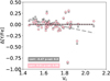 |
Fig. 2 Example of the corrected abundance of [Y/Fe] as a function of Vt for NGC 104. Grey and pink symbols show the raw and corrected abundance, respectively. See the text for details. |
4 Trend with Vt
As noted in the literature (e.g. Worley et al. 2013), strong absorption lines – such as those used to measure yttrium (Y) and barium (Ba) – are often saturated, making their derived abundances highly sensitive to the choice of microturbulence velocity (Vt). We refer the reader to Appendix B to see the effect of Vt on each GCs. To reduce the impact of this dependence, we adopted the approach presented in SUL24, where a linear fit is applied to the original, uncorrected abundances from the Gaia-ESO catalogue (referred to from hereafter as raw) abundance versus Vt trend. The residuals from this fit, defined as Δ[El/Fe], represent the corrected abundance values, where El refers to a given element.
Figure 2 illustrates this method using yttrium in the GC NGC 104 as an example. Grey symbols show the raw [Y/Fe] abundances, while pink symbols represent the corrected values, Δ[Y/Fe]. The figure also highlights the change in the Spearman correlation before and after the correction: the initial strong negative correlation with Vt (corr = −0.47 and p-val=0.00) becomes weak and statistically negligible (p-val = 0.96) after applying the correction. This correction method effectively removes artificial trends with Vt, which could otherwise introduce spurious internal scatter in the abundance distribution within a GC. Importantly, it preserves any genuine internal variations or correlations with other elements. However, because the method relies on an arbitrary zero-point, it does not provide absolute abundances. Therefore, the use of this method is only valid for internal comparisons within a given cluster. For consistency, we applied this correction to all n-capture elements analysed in this study3, including those with weaker lines (e.g. La and Eu), even though such elements are not expected to be particularly sensitive to Vt.
5 Globular clusters in the Galactic context
5.1 Globular clusters as tracers of the Galaxy
Among the interesting aspects of GCs is their ability to track the Galactic populations in a complementary way to the field stars (see e.g. Massari et al. 2019, 2023, 2025). In addition, GCs offer a key advantage over field stars: their ages can be determined with higher precision through isochrone fitting of the entire cluster sequence (see e.g. Chaboyer 1995; Sarajedini et al. 1997; VandenBerg et al. 2013; Massari et al. 2023; Aguado-Agelet et al. 2025; Ceccarelli et al. 2025).
In this section, we aim to construct a large sample of GCs and field stars that covers the typical metallicity range of the Galactic halo, with precise abundances of n-capture elements. Our goal is to compare the behaviour of field stars and clusters, and to contrast these observations with the predictions of a chemical evolution model. To put the observation and models on the same scale, for this comparison, we used the raw average abundances of n-capture elements per cluster. To build our sample of field stars, we used two samples: the first is based on data from the Measuring at Intermediate Metallicity NeutronCapture Elements (MINCE) project (Cescutti et al. 2022), which analysed high-quality spectra homogeneously and consistently, and the second uses the results of the Chemical Evolution of R-process Elements in Stars (CERES) project (Lombardo et al. 2022), including metal-poorer stars ([Fe/H]<−1.5). In particular, the MINCE results are outlined in: the first paper of the collaboration (MINCE I), in which the authors collected spectra of metal-poor stars ([Fe/H]≲−1.5 dex), primarily from the Galactic halo; MINCE II (François et al. 2024), where they expanded their sample to include stars associated with two accreted remnants: Gaia-Sausage Enceladus (GSE) and Sequoia; most recently, MINCE III (Lucertini et al. 2025), in which they extended their study to stars with higher metallicities, up to [Fe/H]=−1.0 dex.
The abundance trends of our combined sample of field stars and GCs are compared with the results of a Galactic chemical evolution model obtained with the GEMS code (Rizzuti et al. 2025), which is based on the stochastic models of Cescutti (2008) and Rizzuti et al. (2021). We refer the reader to Rizzuti et al. (2025) for a description of the model, and for some results for CNO and n-capture elements. Below is a brief overview of the key features and assumptions of the model, while for more details we refer to Cescutti et al. (2015) and Rizzuti et al. (2019, 2021, 2025). Each of the many volumes in the simulations (~10 000) is considered isolated and contains the typical mass of gas swept by a Type II SN explosion. The model can reproduce the evolution of the stars in the Galactic halo, with a total duration of 1 Gyr. For the nucleosynthesis of n-capture elements, the following sources are considered: s-process from fast-rotating massive stars (Limongi & Chieffi 2018); s-process from AGB stars (FRUITY; Cristallo et al. 2011); r-process from neutron star mergers (NSMs) with 1 Myr time delay, with the Ba yields estimated by Cescutti et al. (2013) and the other elements scaled to the solar system r-process (Cescutti & Chiappini 2014). The s-process by rotating massive stars is particularly important in this context, since rotation enables the production of s-process elements up to the second peak even at low metallicity. The question of the production sites of the r-process is still open. However, several works have shown that the synthesis of Eu in the Galaxy can be explained by either only NSMs with a short time delay of 1 Myr or both MRD SNe and NSMs with a longer time delay (see e.g. Matteucci et al. 2014; Cescutti et al. 2015; Molero et al. 2023).
Figure 3 presents the raw average abundance ratios of Y, Zr, Ba, La, Ce, Pr, Nd, and Eu relative to iron in our GC sample (ed dots) as a function of metallicity [Fe/H], together with the sample of field stars from CERES and MINCE. We also added a sample of disc stars from the Gaia-ESO Survey. When available, model predictions are shown with a colour gradient representing the logarithmic number of stars in each bin.
First, both the GC and field star samples exhibit similar trends across all abundance planes, with an increasing spread towards lower metallicities. When comparing model results to observations, it is notable that the stochastic models successfully reproduce both the dispersion arising from the contribution of different nucleosynthesis sites and the overall trend of chemical evolution. Additionally, model predictions suggest (super)solar abundances of [Y/Fe], [Zr/Fe], and [Ba/Fe] (as well as [La/Fe] and [Eu/Fe]) around [Fe/H] = −2.0 dex, followed by a decline at [Fe/H] > −1.5 dex, primarily due to contributions from Type Ia SNe. The observed abundance trends in GCs closely match these predictions, particularly for the s-process elements Y, Ba, and La. A similar agreement is observed for the r-process element Eu. Interestingly, [Zr/Fe] aligns with the upper envelope of the model predictions, indicating a potential systematic offset, likely arising from the models’ underestimation of the r-process contribution to Zr.
5.2 The origin of globular clusters: Hints from n-capture elements
The population of Galactic GCs is known to have a diverse origin, with clusters broadly classified as either in situ or ex situ. We adopted the classification by Massari et al. (2019), who combined kinematic and age information for a large sample of GCs to infer their likely origin. For methodological details, we refer the reader to the original publication. Table 2 summarises the origin of our sample based on this origin classification. As mentioned in Sect. 4, our corrected abundances (Δ[El/Fe]) work only for internal comparisons; therefore, to ensure a consistent comparison between the two groups, we used a slightly different approach. First, we grouped the GCs according to their origin, we filtered stars of each group to only those within a similar range of Vt (ranging from 1.35 and 2.35 km s−1), excluding stars with different Vt values to minimise potential biases in the analysis. Then, we computed a global Δ abundances across each group, defined as Δ[El/Fe]g. The table reports the number of selected stars, the maximum abundance difference (Rx), and the interquartile range (IQRx) for each n-capture element, separated by in situ and ex situ GCs. In general, R x and IQRx values do not reveal significant differences between the two populations. The only exception is Eu, for which the IQRx in in-situ GCs is 0.10 dex larger than in ex situ clusters, suggesting a slightly broader internal variation.
Some studies (e.g. Monty et al. 2024) have suggested that combining r-process elements (e.g. Eu) with α-elements (such as Mg or Si) could provide better insights into the origin of GCs. In particular, [Eu/Si] ratios in field stars with high and low orbital energies – typically associated with extragalactic and Galactic origins, respectively – show distinct patterns. We tested this hypothesis in Fig. 4. The left panels display the raw [Eu/Mg] ratios versus [Fe/H] for our sample, grouped by origin according to Massari et al. (2019). Note that [Eu/Mg] values are not available for a few clusters (NGC 4590, NGC 4833, and NGC 7078). In the figure, in situ and ex situ clusters are represented by black squares and red dots, respectively. While in situ clusters exhibit a broad distribution of [Eu/Mg], ex situ clusters show a flatter, systematically higher distribution at a given metallicity, with an average ratio of 0.14 and 0.32 dex, respectively. This offset likely reflects differences in the chemical enrichment histories of the two samples, consistent with the findings of Matsuno et al. (2021) and Monty et al. (2024). Although one might suspect that the MP phenomenon – particularly Mg variations – could influence this ratio, a comparison with the results of Carretta et al. (2010, see their Table 2) provides clarity. They reported the maximum [Mg/Fe] values found, corresponding to FG stars, for 19 GCs. On average, in situ clusters show Mg abundances approximately 0.10 dex higher than their ex situ counterparts. This supports the observed trend of lower [Eu/Mg] ratios among in situ clusters. The right panel of Fig. 4 presents [Eu/Ca] ratios, where Ca serves as an α-element unaffected by the MP phenomenon. Although the trend is subtler, it shows a similar separation between the two populations, reinforcing the potential of [Eu/α] ratios as tracers of GC origin. The middle panel of Fig. 4 presents the Kolmogorov-Smirnov (K-S) comparison of the cumulative [Eu/Mg] distribution for in situ (black line) and ex situ (red line) GCs. This statistical test evaluates the likelihood that two samples originate from the same parent distribution. In this case, for our limited sample, a prob(K-S) of 0.027 allows us to reject the null hypothesis, reinforcing the conclusion that the [Eu/Mg] ratio effectively distinguishes ex situ GCs.
To confirm independently the chemical diversity of the two populations of GCs, we performed a simple clustering algorithm aiming to identify groups using only the chemical abundance features presented in the Gaia-ESO catalogue. To do so, we used a K-MEANS method (Likas et al. 2003) using the hyperparameter n_cluster equal to 2 in a subset of raw abundances ([Fe/H], [Na/Fe], [Mg/Fe], [Al/Fe], [Y/Fe], [Ba/Fe], [La/Fe], [Ce/Fe], [Eu/Fe], [Si/Fe], [Ca/Fe], [Sc/Fe], [Ti/Fe], [V/Fe], [Cr/Fe], [Mn/Fe], [Co/Fe], [Ni/Fe], [Cu/Fe], and [Zn/Fe]). The results showed that, for all the GCs with available Eu abundances, the clustering algorithm was able to correctly identify the origin label (as provided by Massari et al. 2019) in 10 out of 11 cases, failing only for NGC 1904, for which it determined an in situ origin. This independently confirms that they are chemically distinct.
Statistical summary by origin.
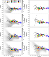 |
Fig. 3 Comparison with Galactic chemical evolution models – when available – with the reported [Y/Fe], [Zr/Fe], [Ba/Fe], [La/Fe], [Ce/Fe], [Pr/Fe], [Nd/Fe], and [Eu/Fe]. The background, coloured in grey, scales with the logarithmic number of stars in each bin. The correspondent abundances of candidate stars of GSE (François et al. 2024; Lucertini et al. 2025), Sequoia (François et al. 2024; Lucertini et al. 2025), Ceres (Lombardo et al. 2021; Lombardo 2023), halo stars (Lucertini et al. 2025), the Gaia-ESO sample of disc stars, and thick disc stars (François et al. 2024; Lucertini et al. 2025) are shown as in blue diamonds, red triangles, black pluses, yellow dots, blue crosses, and black stars, respectively. |
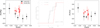 |
Fig. 4 [Eu/Mg] and [Eu/Ca] ratios in the two subsamples. Left: Eu over Mg ratio as a function of [Fe/H]. Middle: K–S comparison of the cumulative distribution of the [Eu/Mg] ratio. Right: Eu over Ca ratio as a function of [Fe/H]. |
6 N-capture abundances and other chemical multi-population indicators
The two elements most commonly used to identify the different stellar populations in GCs are Na and Al. They are produced during hot H-burning and thus are involved in the MP phenomenon. In this analysis, we classify FG stars as those within three times the typical observational Na uncertainty (0.075 dex) from [Na/Fe]lim, which is defined as the raw average [Na/Fe] abundance of the three stars with the lowest [Na/Fe] values. The following paragraphs present our findings on the correlations between light and n-capture element abundances across different stellar populations in GCs.
The presence of possible correlations between the abundances of Na and Al with those of the s-process elements may give us clues as to the nature of polluters that changed the composition of SG stars. Indeed, both Na and Al and s-process elements can be produced in similar environments, particularly in intermediate- to low-mass stars (see e.g. Karakas & Lattanzio 2014) or in massive stars with rotation-induced mixing (see e.g. Limongi & Chieffi 2018). Therefore, a shared origin for the two elements in specific types of stars might lead to a correlation between them. On the other hand, we do not expect correlations between the abundances of Na and Al with those of the r-process elements.
For this study, we assessed the significance of correlations using the p-value from the Spearman statistical method (Spearman 1904). We classified correlations as highly significant for p-values below 0.05, moderately significant for p-values between 0.05 and 0.10, and weak or negligible for p-values greater than 0.10. It is important to note that outlier abundances, which were defined as abundances larger or smaller than 0.5 dex from the average cluster abundance, were excluded from this analysis.
Sodium: Figure 5 shows the abundance of Y as a function of the Na abundances for our sample of GCs. We found mixed results for well-sampled GCs. While some clusters – such as NGC 104, NGC 362, NGC 1851, NGC 6218, and NGC 6752 – exhibited mildly or highly significant correlations, others showed no statistically significant trends. The correlation factors are consistently positive. Figures C.1 and C.2 present the corresponding results for all other analysed n-capture elements, including Zr, Ba, La, Ce, Pr, Nd, and Eu. The other first-peak s-process element, Zr, exhibits a mildly significant positive correlation in two GCs (NGC 104 and NGC 1851). Among the second-peak s-process elements, Ba shows a highly significant positive correlation in NGC 362 and NGC 6218, whereas La does not display any significant correlation in any cluster. Ce exhibits two distinct behaviours: in NGC 6218, it shows a highly significant positive correlation, while in other clusters, its trend is less clear. In contrast, Pr shows no significant correlation. On the other hand, Nd presents a highly significant positive correlation in NGC 1851 and NGC 6218, and a mildly significant one in NGC 362 and NGC 6752. Finally, the r-process element Eu does not exhibit any correlation in any of the studied GCs.
Aluminium: Analogously, we compare the abundances of n-capture elements with those of Al. While Fig. C.3 show the Δ[Y/Fe], Δ[Zr/Fe], Δ[Ba/Fe], and Δ[La/Fe] abundances, Fig. C.4 displays the Δ[Ce/Fe], Δ[Pr/Fe], Δ[Nd/Fe], and Δ[Eu/Fe] abundances as a function of the [Al/Fe] for our sample of GCs. Although in many clusters we did not observe any significant correlation between n-capture element abundances and those of Al, for the case of Δ[Y/Fe], the GCs NGC 104, NGC 1851, NGC 5927, NGC 6218, NGC 6752, and NGC 7089 show a highly significant positive correlation, while NGC 362 and NGC 2808 exhibit a mild correlation. Zr only presents high significant positive correlations in NGC 1261, and a mild one in NGC 104; Ba shows a highly significant positive correlation in NGC 362 and NGC 6218 and a mild one in NGC 6752. La only has a highly significant positive correlation in NGC 104. Ce presents different behaviours, with NGC 104 having a mildly significant positive correlation, a highly significant one in NGC 6218 and a negative, highly significant one in NGC 1904. A similar case for Pr presents a highly significant positive correlation in NGC 104 but a negative one with mild significance in NGC 1904. Nd shows a positive correlation in NGC 104, NGC 1851, NGC 6218, NGC 7078, NGC 7089, and NGC 1261 with high significance in the first five clusters and a mild one in the last one. Finally, Eu exhibits a highly significant negative correlation in NGC 5927 and a positive one in NGC 7089.
Although we found many (anti-)correlations among different pairs of elements, their strengths vary cluster-to-cluster. This means that the Na and Al nucleosynthetic production can affect the nucleosynthesis of n-capture elements in those GCs positively or negatively, depending on the slope of the correlation. We can conclude that, in general, correlations with slow n-capture elements show some associations with Na and Al, while r-process elements like Eu do not. This seems to suggest that slow n-capture elements and light elements like Na and Al could share common nucleosynthesis sites, supporting the hypothesis that AGB stars of different masses and/or massive stars with rotation-induced mixing could contribute to the intra-cluster pollution. On the other hand, the significance and magnitude of these correlations are not always consistent, nor are explainable in nucleosynthetic terms (e.g. La and Ce production is closely associated with that of Ba, and therefore the correlation of one of these elements with Al or Na without a similar behaviour from the other two is of limited astrophysical significance). This may be due to limited sample sizes, variations in behaviour across different metallicities, and potentially unaccounted-for observational uncertainties. Similar results have been reported in the literature; in particular, Yong & Grundahl (2008) found correlations between some light s-process elements and light elements in NGC 1851.
To improve our statistical robustness, we focused on global trends across GCs rather than analysing them individually, following the methodology outlined in SUL24, who explored potential correlations between s-process elements and Na by dividing their sample into three metallicity regimes: metal-poor, mid-metallicity, and metal-rich for which Δ s were determined as a group. These regimes correspond to GCs with metallicities of [Fe/H] < −1.8, −1.8 < [Fe/H] < −1.1, and [Fe/H] > −1.1 dex, respectively. In their study, they reported a slight correlation between Y and Na. To test this in our sample, we applied the same procedure. Figure 6 presents the results for our sample along with the corresponding Spearman correlation coefficients, calculated without including outlier stars. The upper panels display the distribution of Δ[Y/Fe] as a function of [Na/Fe], while the lower panels show the analogous results for Δ[Ba/Fe]. Each panel includes the correlation coefficient and its associated significance, which reflect a strong correlation between Δ[Y/Fe] and [Na/Fe] in all the metallicity regimes. On the other hand, Δ[Ba/Fe] and [Na/Fe] display a significant correlation only in the most metal-rich regime, which disappears while decreasing the metallicity. Our results support those of SUL24, confirming a significant contribution of light s-process elements in the same nucleosynthetic site where Na was produced.
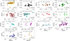 |
Fig. 5 Δ[Y/Fe] abundances as a function of [Na/Fe] for the GCs in our sample. Lighter and darker symbols represent stars belonging to the FG and SG according to our definition (see Sect. 6), respectively. Every panel shows the corresponding Spearman correlation and p-value. |
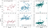 |
Fig. 6 Distribution of the Δ[Y/Fe] (upper panels) and Δ[Ba/Fe] (lower panels) as a function of [Na/Fe] divided by metallicity bins. The metallicity bins from left to right are: [Fe/H]<−1.8, −1.8<[Fe/H]<-1.1, and [Fe/H]>−1.1 dex. |
7 Neutron-capture homogeneity in GCs
The degree of chemical homogeneity within GCs offers valuable clues about their origin. Elements such as Al, Na, and O are known to exhibit significant internal spreads (Carretta et al. 2009), while most heavier elements remain relatively uniform across the majority of GCs, commonly referred to as Type I clusters. In contrast, Type II GCs display more complex abundance patterns, including variations in iron and, in some cases, s-process elements. Based on classifications by Milone et al. (2017) and Nardiello et al. (2018), our sample includes five Type II clusters: NGC 362, NGC 1261, NGC 1851, NGC 7078, and NGC 7089. The remaining clusters are classified as Type I, except NGC 1904 and NGC 4372, which lack definitive classifications. Despite growing interest, evidence of internal variations in n-capture elements within GCs remains limited, with only a few studies, such as the recent analysis of NGC 6341 by Kirby et al. (2023), reporting such findings.
We examined whether the internal abundance spreads differ between the two stellar populations within each GC. To separate the FG and SG stars, we applied the classification described in Sect. 6. Figure 7 displays the average and standard deviation of Δ[El/Fe] for FG (black symbols) and SG (red symbols) stars in each GC and each element. Dashed lines at ±0.15 dex represent a conservative typical error in the measurement of the abundances. Metal-poor clusters such as NGC 4372, NGC 4590, NGC 4833, NGC 7078, and NGC 7089 lack sufficient data to support a robust comparison. While we observed differences in the average abundances between FG and SG populations, these differences typically fall within one standard deviation of each other. This may be due to the division of the sample into sub-populations, which reduces the number of stars in each group and increases statistical uncertainty. Consequently, genuine underlying trends could appear less significant even if a broader correlation is present.
In most Type I GCs, the two populations show comparable spreads. The ratio of the spreads between the SG and FG is about 1, suggesting that n-capture elements are minimally affected by the polluters responsible for the MP phenomenon. For Type II GCs – specifically in GCs with larger number statistics (NGC 362, NGC 1261, and NGC 1851) – the SG stars consistently show larger spreads in s-process elements, having on average a spread ratio between the two populations generation of about twice larger than Type I GCs, indicating the contribution from polluters to the chemical enrichment of the clusters. These finding supports previous studies that reported spread in s-process elements in NGC 362 (e.g. Monty et al. 2023) and NGC 1851 (Carretta et al. 2011). In the case of NGC 1261, neither Koch-Hansen et al. (2021) nor Marino et al. (2021) found significant spreads in s-process elements. Nevertheless, Koch-Hansen et al. (2021) reported a peculiar overabundance of r-process elements, which may also contribute, to some extent, to the production of s-process elements.
Further analysis using differential analysis techniques (e.g. Monty et al. 2023) is effective in overcoming current measurement uncertainties, contributing to a more precise determination of the internal variation in GCs. In the longer term, high-resolution, multi-object spectrographs will be essential to fully explore these subtle chemical variations. Instruments like the proposed high-resolution multi-object spectrograph (HRMOS) (Magrini et al. 2023) will enable precise abundance determinations for a wide range of n-capture elements in GC stars, including elements of the third peak, like Pb, offering deeper insights into the nature and contributions of intra-cluster polluters.
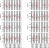 |
Fig. 7 Average and standard deviation for Δ[El/Fe] per GC. They are grouped by generation, with black and red symbols for FG and SG stars, respectively. White and grey areas are plotted only to facilitate the figure’s readability and do not have further meaning. Dashed lines at ±0.15 dex represent the typical uncertainty in the abundance measurements. |
8 Summary and conclusions
We utilised the GC sample of the Gaia-ESO Survey to investigate the abundances of n-capture elements. First, we analysed the abundances of Y, Zr, Ba, La, Ce, Nd, Pr, and Eu to trace the chemical composition of the Galaxy. We combined our results with those of field stars (MINCE and CERES samples) and compared them with the results of a stochastic chemical evolution model of the Milky Way halo (Rizzuti et al. 2025). Then, we aimed to differentiate the origins of these clusters by examining [Eu/Mg], a ratio that reflects the distinct chemical enrichment histories of their birth environments. Next, we explored potential relationships between hot H-burning elements – commonly used as tracers of MPs in GCs – and heavier elements to gain insights into the nature of the stars responsible for intracluster pollution. Finally, we investigated the homogeneity of GCs in n-capture abundances, considering also their FG and SG stars separately. Below, we summarise our key findings:
(i) Most GCs in our sample closely follow the chemical distribution of halo and disc field stars with similar metallicity across all analysed n-capture elements. In addition, model predictions generally align well with the observed trends for most elements. The main exception is Zr, for which observations cover the upper envelope of the model predictions, likely due to an underestimation of the r-process contribution to Zr nucleosynthesis.
(ii) The [Eu/Mg] ratio appears to be a useful indicator of GC origin, at least in distinguishing in situ from ex situ clusters, reflecting the different chemical enrichment histories of their formation environments. This finding reinforces previous results in the literature. The classification of GCs based on their chemical properties was further supported by a clustering algorithm, which successfully recovered the origin labels for most of the samples for which Eu measurements were available. However, a larger GC sample covering a wider metallicity range is needed to confirm this trend.
(iii) We explored n-capture element abundances in relation to Na and Al, which are typically used as tracers of MPs in GCs. Some clusters, such as NGC 104, NGC 1851, NGC 6218, and NGC 6752, displayed strong correlations between the light s-process element Y and Na. Similarly, for clusters like NGC 362 and NGC 6218 there was a significant correlation between the heavier s-process element Ba and Na. However, no correlations were found with the r-process element Eu. We divided the GC sample into different metallicity bins – low-metallicity ([Fe/H] < −1.8), intermediate-metallicity (−1.8 < [Fe/H] < −1.1), and high-metallicity ([Fe/H] > −1.1 dex) – and observe a strong correlation between Y and Na in all three regimes. These results suggest that light s-process elements might have been synthesised in the same nucleosynthetic sites as Na, with the strength of their contribution varying based on the mass and metallicity of the polluter(s), which could be AGB stars and/or fast-rotating massive stars.
(iv) Finally, we find no strong evidence of systematic differences in abundance spreads between FG and SG stars in Type I GCs. In contrast, in Type II GCs with large sample sizes, such as NGC 362, NGC 1261, and NGC 1851, SG stars consistently exhibit larger spreads in s-process element abundances compared to FG stars, suggesting a possible influence from internal polluters.
It is important to note that internal abundance spreads in GCs are often subtle, making them difficult to detect given observational uncertainties. Therefore, we emphasise the need for a high-resolution multi-object spectrograph, such as HRMOS, to overcome these limitations and provide more precise measurements.
Data availability
The table with the corrected abundances is available at the CDS via anonymous ftp to cdsarc.cds.unistra.fr (130.79.128.5) or via https://cdsarc.cds.unistra.fr/viz-bin/cat/J/A+A/699/A41
Acknowledgements
J.S.U., L.M., S.R., G.C., F.R. and L.B. thank INAF for the support (Large Grant EPOCH), the Mini-Grants Checs (1.05.23.04.02), and the financial support under the National Recovery and Resilience Plan (NRRP), Mission 4, Component 2, Investment 1.1, Call for tender No. 104 published on 2.2.2022 by the Italian Ministry of University and Research (MUR), funded by the European Union – NextGenerationEU – Project ‘Cosmic POT’ Grant Assignment Decree No. 2022X4TM3H by the Italian Ministry of the University and Research (MUR). J.S.U. thanks INAF for the support through the Mini-Grant (1.05.24.07.02). FR is a fellow of the Alexander von Humboldt Foundation. FR acknowledges support by the Klaus Tschira Foundation. Based on data products from observations made with ESO Telescopes at the La Silla Paranal Observatory under programmes 188.B-3002, 193.B-0936, and 197.B-1074. The Gaia-ESO final data release DR5.1 is available from the ESO webpage.
Appendix A Comparison with the literature
We compared the results of Gaia-ESO DR5.1 with the literature ones. To this aim, we used the results of the spectroscopic analysis done by Carretta et al. (2009, hereafter C09u), who analysed more than 200 stars in 18 GCs using UVES spectra. For these spectra, they obtained stellar parameters and abundances of Na, Mg, Al, and Si. Moreover, SUL24 extended the analysis to n-capture elements using the same sample and adopting their stellar parameters. There are 48 stars in 6 GCs in both the mentioned sample and our Gaia-ESO sample. We compared their stellar parameters as well as the abundances of Na, Mg, Al, and Si from C09u and Y, Ba, La, and Eu from SUL24. In addition, we added the GCs NGC 1851 (Carretta et al. 2011), NGC 362 (Carretta et al. 2013), and NGC 4833 (Carretta et al. 2014), which were analysed in an analogous way to the aforementioned articles. In this set of GCs, there are 37 stars that are also in the Gaia-ESO sample, and their stellar parameters and abundances of Na, Mg, Al, Si, Y, Ba, La, and Eu were measured.
Figure A.1 shows the Teff, log g, [Fe/H], and microturbulence velocity (Vt) reported by Gaia-ESO DR5.1 and their corresponding results obtained by C09u, Carretta et al. (2011), Carretta et al. (2013), and Carretta et al. (2014). Each panel displays the stars in common, colour-coded by GC, along with the mean (μ) and standard deviation (σ) of the differences between the literature and Gaia-ESO values. The panels show that there is a systematic difference towards higher Teff and log g in the results derived by Gaia-ESO. It is worth noticing that the Teff reported by C09u were obtained using photometric relations, and the log g were obtained using the mentioned Teff along with the corresponding bolometric corrections. Therefore, those systematic differences could be due to the different methods used for their determination.
There is no clear correlation between the two Vt determinations because both cover a small range and remain nearly constant. This is due to the sample being almost entirely composed of red giant stars with similar Vt values. However, on average, the Vt values of Gaia-ESO are 0.13 higher than the ones reported in C09u, which is about their typical internal error found in the Vt determination.
Figure A.2 displays the comparison of [Na/H], [Mg/H], [Al/H], and [Si/H] normalised to the Sun for the in-common stars. On average, the Gaia-ESO DR5.1 results agree with the literature. It is worth noticing that upper limits (triangle symbols) reported by C09u were not used for the computation of the mean and standard deviation of the results’ difference. In general, all the species follow closely the one-to-one relation. [Na/H] and [Si/H] from Gaia-ESO show systematically lower abundance, which could be due to the higher Teff and log g4. The [Mg/H] and [Al/H] abundances of Gaia-ESO are slightly higher in comparison with the literature, which might be due to the slightly higher Teff computed by the survey.
Finally, Fig. A.3 shows the comparison of n-capture elements reported by SUL24 and Carretta et al. (2011, 2013, 2014), when available. The figure reveals that Gaia-ESO DR5.1 and the literature follow the same trend for the most populated species– however, with a larger spread with respect to the lighter elements. The larger difference is reported for the abundances of [Y/H], [Ba/H], [Eu/H], where the Gaia-ESO DR5.1 found higher abundances with respect to the literature. The difference is likely primarily due to the high sensitivity of Y and Ba abundances to stellar parameters (the clear Teff offset and the different Vt distribution), with an additional contribution from the different line lists used.
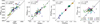 |
Fig. A.1 Comparison of the stellar parameters reported by C09u, Carretta et al. (2011), Carretta et al. (2013), Carretta et al. (2014), SUL24, and the Gaia-ESO DR5.1 for in-common stars. Each panel shows the mean and standard deviation of the difference between the result obtained by Gaia-ESO and C09u. |
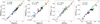 |
Fig. A.2 Comparison of the (from left to right) [Na/H], [Mg/H], [Al/H], and [Si/H] reported by C09u, Carretta et al. (2011), Carretta et al. (2013), Carretta et al. (2014), SUL24, and the Gaia-ESO DR5.1 for in-common stars. Coloured dots and triangles represent actual measurements and upper limits, respectively. The present figure follows the same description as Fig. A.1. |
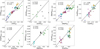 |
Fig. A.3 Comparison of the abundance of (from left to right) [Y/H], [Zr/H], [Ba/H], [La/H], [Ce/H], [Nd/H], and [Eu/H] reported by SUL24, Carretta et al. (2013, 2011, 2014), and the Gaia-ESO DR5.1 for in-common stars. The figure follows the same description as Fig. A.2. |
Appendix B Effect of Vt on Y and Ba in our GC sample
As mentioned in Sect. 4, strong lines such as those of Y and Ba are often saturated and highly sensitive to Vt, thus leading to a wrong abundance determination of these species. To illustrate how this trend affects the whole sample of GCs, Fig. B.1 displays the abundances of [Y/Fe] (panels on the left) and [Ba/Fe] (panels on the right) as a function of Vt for each GC. Additionally, each panel displays the corresponding linear fit equation and Spearman statistics. As shown in the figure, some clusters, such as NGC 1904, exhibit a strong dependence of both yttrium and barium abundances on Vt, with slopes of −0.62 and −0.54, respectively. This leads to internal cluster variations of approximately 0.50 dex in [Y/Fe] and 0.35 dex in [Ba/Fe] within its Vt range. In contrast, other clusters exhibit negligible slopes, suggesting minimal or no dependence on Vt. A quick comparison between two GCs — one with a strong Y trend (NGC 1904) and one with a weak Y trend (NGC 7078) — reveals that the cluster with the stronger trend also spans a wider range of Teff and log g.
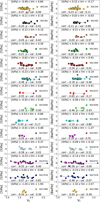 |
Fig. B.1 [Y/Fe] and [Ba/Fe] abundances as a function of Vt for the whole sample of GCs. Every panel displays the one-degree fit’s equation and the respective Spearman correlation and p-value. |
Appendix C Additional n-capture elements and MP indicator trends
As discussed in Sect. 6, we examined possible correlations between the n-capture elements analysed in this work and the commonly used MP indicators Na and Al. Figures C.1 and C.2 show the abundances of various n-capture elements as a function of Na, while Figs. C.3 and C.4 present the corresponding plots for Al. A detailed interpretation of these trends is provided in Sect. 6.
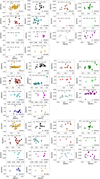 |
Fig. C.1 Abundances of Δ[Zr/Fe], Δ[Ba/Fe], and Δ[La/Fe] as a function of [Na/Fe] for GCs in our sample. Every panel shows the corresponding Spearman correlation and p-value. |
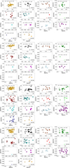 |
Fig. C.2 Abundances of Δ[Ce/Fe], Δ[Pr/Fe], Δ[Nd/Fe], and Δ[Eu/Fe] as a function of [Na/Fe] for GCs in our sample. Every panel shows the corresponding Spearman correlation and p-value. |
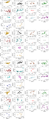 |
Fig. C.3 Abundances of Δ[Y/Fe], Δ[Zr/Fe], Δ[Ba/Fe], and Δ[La/Fe] as a function of [Al/Fe] for GCs in our sample. Every panel shows the corresponding Spearman correlation and p-value. |
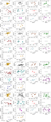 |
Fig. C.4 Abundances of Δ[Ce/Fe], Δ[Pr/Fe], Δ[Nd/Fe], and Δ[Eu/Fe] as a function of [Al/Fe] for GCs in our sample. Every panel shows the corresponding Spearman correlation and p-value. |
References
- Aguado-Agelet, F., Massari, D., Monelli, M., et al. 2025, A&A, submitted [NASA ADS] [CrossRef] [EDP Sciences] [Google Scholar]
- Asplund, M., Grevesse, N., Sauval, A. J., & Scott, P. 2009, ARA&A, 47, 481 [NASA ADS] [CrossRef] [Google Scholar]
- Bastian, N., & Lardo, C. 2018, ARA&A, 56, 83 [Google Scholar]
- Bressan, A., Marigo, P., Girardi, L., et al. 2012, MNRAS, 427, 127 [NASA ADS] [CrossRef] [Google Scholar]
- Buder, S., Lind, K., Ness, M. K., et al. 2019, A&A, 624, A19 [NASA ADS] [CrossRef] [EDP Sciences] [Google Scholar]
- Carretta, E., & Bragaglia, A. 2022, A&A, 660, L1 [NASA ADS] [CrossRef] [EDP Sciences] [Google Scholar]
- Carretta, E., Bragaglia, A., Gratton, R., & Lucatello, S. 2009, A&A, 505, 139 [NASA ADS] [CrossRef] [EDP Sciences] [Google Scholar]
- Carretta, E., Bragaglia, A., Gratton, R. G., et al. 2010, A&A, 516, A55 [NASA ADS] [CrossRef] [EDP Sciences] [Google Scholar]
- Carretta, E., Lucatello, S., Gratton, R. G., Bragaglia, A., & D’Orazi, V. 2011, A&A, 533, A69 [NASA ADS] [CrossRef] [EDP Sciences] [Google Scholar]
- Carretta, E., Bragaglia, A., Gratton, R. G., et al. 2013, A&A, 557, A138 [NASA ADS] [CrossRef] [EDP Sciences] [Google Scholar]
- Carretta, E., Bragaglia, A., Gratton, R. G., et al. 2014, A&A, 564, A60 [NASA ADS] [CrossRef] [EDP Sciences] [Google Scholar]
- Ceccarelli, E., Massari, D., Aguado-Agelet, F., et al. 2025, A&A, submitted [Google Scholar]
- Cescutti, G. 2008, A&A, 481, 691 [NASA ADS] [CrossRef] [EDP Sciences] [Google Scholar]
- Cescutti, G., & Chiappini, C. 2014, A&A, 565, A51 [NASA ADS] [CrossRef] [EDP Sciences] [Google Scholar]
- Cescutti, G., Chiappini, C., Hirschi, R., Meynet, G., & Frischknecht, U. 2013, A&A, 553, A51 [NASA ADS] [CrossRef] [EDP Sciences] [Google Scholar]
- Cescutti, G., Romano, D., Matteucci, F., Chiappini, C., & Hirschi, R. 2015, A&A, 577, A139 [NASA ADS] [CrossRef] [EDP Sciences] [Google Scholar]
- Cescutti, G., Bonifacio, P., Caffau, E., et al. 2022, A&A, 668, A168 [NASA ADS] [CrossRef] [EDP Sciences] [Google Scholar]
- Chaboyer, B. 1995, ApJ, 444, L9 [Google Scholar]
- Cohen, J. G. 2011, ApJ, 740, L38 [NASA ADS] [CrossRef] [Google Scholar]
- Cowan, J. J., Sneden, C., Lawler, J. E., et al. 2021, Rev. Mod. Phys., 93, 015002 [Google Scholar]
- Cristallo, S., Piersanti, L., Straniero, O., et al. 2011, ApJS, 197, 17 [NASA ADS] [CrossRef] [Google Scholar]
- De Angeli, F., Piotto, G., Cassisi, S., et al. 2005, AJ, 130, 116 [NASA ADS] [CrossRef] [Google Scholar]
- de Mink, S. E., Pols, O. R., Langer, N., & Izzard, R. G. 2009, A&A, 507, L1 [NASA ADS] [CrossRef] [EDP Sciences] [Google Scholar]
- Denissenkov, P. A., VandenBerg, D. A., Hartwick, F. D. A., et al. 2015, MNRAS, 448, 3314 [Google Scholar]
- D’Orazi, V., & Marino, A. F. 2010, ApJ, 716, L166 [Google Scholar]
- D’Orazi, V., Gratton, R., Lucatello, S., et al. 2010, ApJ, 719, L213 [CrossRef] [Google Scholar]
- D’Orazi, V., Angelou, G. C., Gratton, R. G., et al. 2014, ApJ, 791, 39 [CrossRef] [Google Scholar]
- D’Orazi, V., Gratton, R. G., Angelou, G. C., et al. 2015, ApJ, 801, L32 [CrossRef] [Google Scholar]
- Fernández-Trincado, J. G., Beers, T. C., Barbuy, B., et al. 2021, ApJ, 918, L9 [CrossRef] [Google Scholar]
- Fernández-Trincado, J. G., Villanova, S., Geisler, D., et al. 2022, A&A, 658, A116 [NASA ADS] [CrossRef] [EDP Sciences] [Google Scholar]
- Forbes, D. A., & Bridges, T. 2010, MNRAS, 404, 1203 [NASA ADS] [Google Scholar]
- François, P., Cescutti, G., Bonifacio, P., et al. 2024, A&A, 686, A295 [NASA ADS] [CrossRef] [EDP Sciences] [Google Scholar]
- Frischknecht, U., Hirschi, R., & Thielemann, F. K. 2012, A&A, 538, L2 [NASA ADS] [CrossRef] [EDP Sciences] [Google Scholar]
- Gaia Collaboration (Brown, A. G. A., et al.) 2021, A&A, 649, A1 [NASA ADS] [CrossRef] [EDP Sciences] [Google Scholar]
- Gilmore, G., Randich, S., Worley, C. C., et al. 2022, A&A, 666, A120 [NASA ADS] [CrossRef] [EDP Sciences] [Google Scholar]
- Gratton, R., Bragaglia, A., Carretta, E., et al. 2019, A&A Rev., 27, 8 [NASA ADS] [CrossRef] [Google Scholar]
- Harris, W. E. 2010, arXiv e-prints [arXiv:1012.3224] [Google Scholar]
- Heiter, U., Lind, K., Bergemann, M., et al. 2020, VizieR On-line Data Catalog: J/A+A/645/A106 [Google Scholar]
- Hourihane, A., François, P., Worley, C. C., et al. 2023, A&A, 676, A129 [NASA ADS] [CrossRef] [EDP Sciences] [Google Scholar]
- Jackson, R. J., Jeffries, R. D., Wright, N. J., et al. 2022, MNRAS, 509, 1664 [Google Scholar]
- James, G., François, P., Bonifacio, P., et al. 2004, A&A, 427, 825 [NASA ADS] [CrossRef] [EDP Sciences] [Google Scholar]
- Karakas, A. I., & Lattanzio, J. C. 2014, PASA, 31, e030 [NASA ADS] [CrossRef] [Google Scholar]
- Kirby, E. N., Ji, A. P., & Kovalev, M. 2023, ApJ, 958, 45 [Google Scholar]
- Koch-Hansen, A. J., Hansen, C. J., & McWilliam, A. 2021, A&A, 653, A2 [NASA ADS] [CrossRef] [EDP Sciences] [Google Scholar]
- Lardo, C., Pancino, E., Bellazzini, M., et al. 2015, A&A, 573, A115 [NASA ADS] [CrossRef] [EDP Sciences] [Google Scholar]
- Likas, A., Vlassis, N., & J. Verbeek, J. 2003, Pattern Recognit., 36, 451 [Google Scholar]
- Limongi, M., & Chieffi, A. 2018, ApJS, 237, 13 [NASA ADS] [CrossRef] [Google Scholar]
- Lombardo, L. 2023, Memorie della Societa Astronomica Italiana, 94, 99 [NASA ADS] [Google Scholar]
- Lombardo, L., François, P., Bonifacio, P., et al. 2021, A&A, 656, A155 [NASA ADS] [CrossRef] [EDP Sciences] [Google Scholar]
- Lombardo, L., Bonifacio, P., François, P., et al. 2022, A&A, 665, A10 [NASA ADS] [CrossRef] [EDP Sciences] [Google Scholar]
- Lucertini, F., Sbordone, L., Caffau, E., et al. 2025, A&A, 695, A36 [NASA ADS] [CrossRef] [EDP Sciences] [Google Scholar]
- Magrini, L., Spina, L., Randich, S., et al. 2018, A&A, 617, A106 [NASA ADS] [CrossRef] [EDP Sciences] [Google Scholar]
- Magrini, L., Bensby, T., Brucalassi, A., et al. 2023, arXiv e-prints [arXiv:2312.08270] [Google Scholar]
- Majewski, S. R., Schiavon, R. P., Frinchaboy, P. M., et al. 2017, AJ, 154, 94 [NASA ADS] [CrossRef] [Google Scholar]
- Marino, A. F., Milone, A. P., Renzini, A., et al. 2021, ApJ, 923, 22 [CrossRef] [Google Scholar]
- Massari, D., Aguado-Agelet, F., Monelli, M., et al. 2023, A&A, 680, A20 [NASA ADS] [CrossRef] [EDP Sciences] [Google Scholar]
- Massari, D., Koppelman, H. H., & Helmi, A. 2019, A&A, 630, L4 [NASA ADS] [CrossRef] [EDP Sciences] [Google Scholar]
- Massari, D., Bellazzini, M., Libralato, M., et al. 2025, A&A, 698, A197 [NASA ADS] [CrossRef] [EDP Sciences] [Google Scholar]
- Matsuno, T., Hirai, Y., Tarumi, Y., et al. 2021, A&A, 650, A110 [NASA ADS] [CrossRef] [EDP Sciences] [Google Scholar]
- Matteucci, F., Romano, D., Arcones, A., Korobkin, O., & Rosswog, S. 2014, MNRAS, 438, 2177 [Google Scholar]
- Meynet, G., Ekström, S., & Maeder, A. 2006, A&A, 447, 623 [NASA ADS] [CrossRef] [EDP Sciences] [Google Scholar]
- Milone, A. P., Piotto, G., Renzini, A., et al. 2017, MNRAS, 464, 3636 [Google Scholar]
- Molero, M., Magrini, L., Matteucci, F., et al. 2023, MNRAS, 523, 2974 [NASA ADS] [CrossRef] [Google Scholar]
- Molero, M., Magrini, L., Palla, M., et al. 2025, A&A, 694, A274 [NASA ADS] [CrossRef] [EDP Sciences] [Google Scholar]
- Monaco, L., Villanova, S., Carraro, G., Mucciarelli, A., & Moni Bidin, C. 2018, A&A, 616, A181 [NASA ADS] [CrossRef] [EDP Sciences] [Google Scholar]
- Monty, S., Yong, D., Marino, A. F., et al. 2023, MNRAS, 518, 965 [Google Scholar]
- Monty, S., Belokurov, V., Sanders, J. L., et al. 2024, MNRAS, 533, 2420 [NASA ADS] [CrossRef] [Google Scholar]
- Nardiello, D., Milone, A. P., Piotto, G., et al. 2018, MNRAS, 477, 2004 [NASA ADS] [CrossRef] [Google Scholar]
- Nishimura, N., Takiwaki, T., & Thielemann, F.-K. 2015, ApJ, 810, 109 [Google Scholar]
- Pancino, E. 2018, A&A, 614, A80 [NASA ADS] [CrossRef] [EDP Sciences] [Google Scholar]
- Pancino, E., Lardo, C., Altavilla, G., et al. 2017a, A&A, 598, A5 [NASA ADS] [CrossRef] [EDP Sciences] [Google Scholar]
- Pancino, E., Romano, D., Tang, B., et al. 2017b, A&A, 601, A112 [NASA ADS] [CrossRef] [EDP Sciences] [Google Scholar]
- Pasquini, L., Avila, G., Blecha, A., et al. 2002, The Messenger, 110, 1 [Google Scholar]
- Perego, A., Thielemann, F. K., & Cescutti, G. 2021, in Handbook of Gravitational Wave Astronomy, eds. C. Bambi, S. Katsanevas, & K. D. Kokkotas (Springer, Singapore), 13 [Google Scholar]
- Randich, S., Gilmore, G., Magrini, L., et al. 2022, A&A, 666, A121 [NASA ADS] [CrossRef] [EDP Sciences] [Google Scholar]
- Rizzuti, F., Cescutti, G., Matteucci, F., et al. 2019, MNRAS, 489, 5244 [NASA ADS] [Google Scholar]
- Rizzuti, F., Cescutti, G., Matteucci, F., et al. 2021, MNRAS, 502, 2495 [NASA ADS] [CrossRef] [Google Scholar]
- Rizzuti, F., Cescutti, G., Molaro, P., et al. 2025, A&A, 698, A118 [NASA ADS] [CrossRef] [EDP Sciences] [Google Scholar]
- Sacco, G. G., Morbidelli, L., Franciosini, E., et al. 2014, A&A, 565, A113 [NASA ADS] [CrossRef] [EDP Sciences] [Google Scholar]
- Salinas, R., & Strader, J. 2015, ApJ, 809, 169 [CrossRef] [Google Scholar]
- Sarajedini, A., Chaboyer, B., & Demarque, P. 1997, PASP, 109, 1321 [NASA ADS] [CrossRef] [Google Scholar]
- Schiappacasse-Ulloa, J., & Lucatello, S. 2023, MNRAS, 520, 5938 [NASA ADS] [CrossRef] [Google Scholar]
- Schiappacasse-Ulloa, J., Lucatello, S., Rain, M. J., & Pietrinferni, A. 2022, MNRAS, 511, 231 [NASA ADS] [CrossRef] [Google Scholar]
- Schiappacasse-Ulloa, J., Lucatello, S., Cescutti, G., & Carretta, E. 2024, A&A, 685, A10 [NASA ADS] [CrossRef] [EDP Sciences] [Google Scholar]
- Siegel, D. M., Barnes, J., & Metzger, B. D. 2019, Nature, 569, 241 [Google Scholar]
- Smiljanic, R., Korn, A. J., Bergemann, M., et al. 2014, A&A, 570, A122 [NASA ADS] [CrossRef] [EDP Sciences] [Google Scholar]
- Spearman, C. 1904, Am. J. Psychol., 15, 72 [Google Scholar]
- Tautvaišienė, G., Drazdauskas, A., Bragaglia, A., et al. 2022, A&A, 658, A80 [CrossRef] [EDP Sciences] [Google Scholar]
- Van der Swaelmen, M., Viscasillas Vázquez, C., Cescutti, G., et al. 2023, A&A, 670, A129 [NASA ADS] [CrossRef] [EDP Sciences] [Google Scholar]
- VandenBerg, D. A., Brogaard, K., Leaman, R., & Casagrande, L. 2013, ApJ, 775, 134 [Google Scholar]
- Vasiliev, E., & Baumgardt, H. 2021, MNRAS, 505, 5978 [NASA ADS] [CrossRef] [Google Scholar]
- Ventura, P., D’Antona, F., Mazzitelli, I., & Gratton, R. 2001, ApJ, 550, L65 [CrossRef] [Google Scholar]
- Worley, C. C., Hill, V., Sobeck, J., & Carretta, E. 2013, A&A, 553, A47 [NASA ADS] [CrossRef] [EDP Sciences] [Google Scholar]
- Worley, C. C., Smiljanic, R., Magrini, L., et al. 2024, A&A, 684, A148 [NASA ADS] [CrossRef] [EDP Sciences] [Google Scholar]
- Yong, D., & Grundahl, F. 2008, ApJ, 672, L29 [NASA ADS] [CrossRef] [Google Scholar]
Median signal-to-noise per pixel over the whole spectrum.
The corrected abundances used in the present analysis are available in electronic format. See the ‘Data availability’ section.
We made sure to report both sets of abundances on the same solar scale.
All Tables
All Figures
|
Fig. 1 Membership selection for NGC 362. The properties of members and non-members are represented with magenta and grey dots, respectively. From left to right: [Fe/H]-parallax, proper motions, and colour–magnitude diagram. In the rightmost panel, we overplot in blue the corresponding isochrone corresponding to [Fe/H]=−1.13 dex, [α/Fe], E(B-V)=0.05, (m-M)V=14.83, and an age of 10.75 Gyr. |
| In the text | |
|
Fig. 2 Example of the corrected abundance of [Y/Fe] as a function of Vt for NGC 104. Grey and pink symbols show the raw and corrected abundance, respectively. See the text for details. |
| In the text | |
|
Fig. 3 Comparison with Galactic chemical evolution models – when available – with the reported [Y/Fe], [Zr/Fe], [Ba/Fe], [La/Fe], [Ce/Fe], [Pr/Fe], [Nd/Fe], and [Eu/Fe]. The background, coloured in grey, scales with the logarithmic number of stars in each bin. The correspondent abundances of candidate stars of GSE (François et al. 2024; Lucertini et al. 2025), Sequoia (François et al. 2024; Lucertini et al. 2025), Ceres (Lombardo et al. 2021; Lombardo 2023), halo stars (Lucertini et al. 2025), the Gaia-ESO sample of disc stars, and thick disc stars (François et al. 2024; Lucertini et al. 2025) are shown as in blue diamonds, red triangles, black pluses, yellow dots, blue crosses, and black stars, respectively. |
| In the text | |
|
Fig. 4 [Eu/Mg] and [Eu/Ca] ratios in the two subsamples. Left: Eu over Mg ratio as a function of [Fe/H]. Middle: K–S comparison of the cumulative distribution of the [Eu/Mg] ratio. Right: Eu over Ca ratio as a function of [Fe/H]. |
| In the text | |
|
Fig. 5 Δ[Y/Fe] abundances as a function of [Na/Fe] for the GCs in our sample. Lighter and darker symbols represent stars belonging to the FG and SG according to our definition (see Sect. 6), respectively. Every panel shows the corresponding Spearman correlation and p-value. |
| In the text | |
|
Fig. 6 Distribution of the Δ[Y/Fe] (upper panels) and Δ[Ba/Fe] (lower panels) as a function of [Na/Fe] divided by metallicity bins. The metallicity bins from left to right are: [Fe/H]<−1.8, −1.8<[Fe/H]<-1.1, and [Fe/H]>−1.1 dex. |
| In the text | |
|
Fig. 7 Average and standard deviation for Δ[El/Fe] per GC. They are grouped by generation, with black and red symbols for FG and SG stars, respectively. White and grey areas are plotted only to facilitate the figure’s readability and do not have further meaning. Dashed lines at ±0.15 dex represent the typical uncertainty in the abundance measurements. |
| In the text | |
|
Fig. A.1 Comparison of the stellar parameters reported by C09u, Carretta et al. (2011), Carretta et al. (2013), Carretta et al. (2014), SUL24, and the Gaia-ESO DR5.1 for in-common stars. Each panel shows the mean and standard deviation of the difference between the result obtained by Gaia-ESO and C09u. |
| In the text | |
|
Fig. A.2 Comparison of the (from left to right) [Na/H], [Mg/H], [Al/H], and [Si/H] reported by C09u, Carretta et al. (2011), Carretta et al. (2013), Carretta et al. (2014), SUL24, and the Gaia-ESO DR5.1 for in-common stars. Coloured dots and triangles represent actual measurements and upper limits, respectively. The present figure follows the same description as Fig. A.1. |
| In the text | |
|
Fig. A.3 Comparison of the abundance of (from left to right) [Y/H], [Zr/H], [Ba/H], [La/H], [Ce/H], [Nd/H], and [Eu/H] reported by SUL24, Carretta et al. (2013, 2011, 2014), and the Gaia-ESO DR5.1 for in-common stars. The figure follows the same description as Fig. A.2. |
| In the text | |
|
Fig. B.1 [Y/Fe] and [Ba/Fe] abundances as a function of Vt for the whole sample of GCs. Every panel displays the one-degree fit’s equation and the respective Spearman correlation and p-value. |
| In the text | |
|
Fig. C.1 Abundances of Δ[Zr/Fe], Δ[Ba/Fe], and Δ[La/Fe] as a function of [Na/Fe] for GCs in our sample. Every panel shows the corresponding Spearman correlation and p-value. |
| In the text | |
|
Fig. C.2 Abundances of Δ[Ce/Fe], Δ[Pr/Fe], Δ[Nd/Fe], and Δ[Eu/Fe] as a function of [Na/Fe] for GCs in our sample. Every panel shows the corresponding Spearman correlation and p-value. |
| In the text | |
|
Fig. C.3 Abundances of Δ[Y/Fe], Δ[Zr/Fe], Δ[Ba/Fe], and Δ[La/Fe] as a function of [Al/Fe] for GCs in our sample. Every panel shows the corresponding Spearman correlation and p-value. |
| In the text | |
|
Fig. C.4 Abundances of Δ[Ce/Fe], Δ[Pr/Fe], Δ[Nd/Fe], and Δ[Eu/Fe] as a function of [Al/Fe] for GCs in our sample. Every panel shows the corresponding Spearman correlation and p-value. |
| In the text | |
Current usage metrics show cumulative count of Article Views (full-text article views including HTML views, PDF and ePub downloads, according to the available data) and Abstracts Views on Vision4Press platform.
Data correspond to usage on the plateform after 2015. The current usage metrics is available 48-96 hours after online publication and is updated daily on week days.
Initial download of the metrics may take a while.