| Issue |
A&A
Volume 685, May 2024
|
|
|---|---|---|
| Article Number | A10 | |
| Number of page(s) | 22 | |
| Section | Galactic structure, stellar clusters and populations | |
| DOI | https://doi.org/10.1051/0004-6361/202348805 | |
| Published online | 30 April 2024 | |
Heavy element abundances in galactic globular clusters⋆
1
Dipartimento di Fisica e Astronomia, Università di Padova, Vicolo dell’Osservatorio 3, 35122 Padova, Italy
e-mail: This email address is being protected from spambots. You need JavaScript enabled to view it.
2
INAF–Osservatorio Astronomico di Padova, Vicolo dell’Osservatorio 5, 35122 Padova, Italy
3
Institute for Advanced Studies, Technische Universität München, Lichtenbergstraße 2a, 85748 Garching bei München, Germany
4
Dipartimento di Fisica, Sezione di Astronomia, Università di Trieste, Via G. B. Tiepolo 11, 34143 Trieste, Italy
5
INAF–Osservatorio Astronomico di Trieste, Via G. B. Tiepolo 11, 34131 Trieste, Italy
6
INFN, Sezione di Trieste, Via A. Valerio 2, 34127 Trieste, Italy
7
INAF–Osservatorio di Astrofisica e Scienza dello Spazio di Bologna, Via Gobetti 93/3, 40129 Bologna, Italy
Received:
30
November
2023
Accepted:
8
February
2024
Abstract
Context. Globular clusters are considered key objects for understanding the formation and evolution of the Milky Way. In this sense, the characterisation of their chemical and orbital parameters can provide constraints on chemical evolution models of the Galaxy.
Aims. We use the heavy element abundances of globular clusters to trace their overall behaviour in the Galaxy, with the aim to analyse potential relations between the hot H-burning and s-process elements.
Methods. We measured the content of Cu I and s- and r-process elements (Y II, Ba II, La II, and Eu II) in a sample of 210 giant stars in 18 galactic globular clusters from high-quality UVES spectra. These clusters span a broad metallicity range and the sample is the largest that has been uniformly analysed to date, with respect to heavy elements in globular clusters.
Results. The Cu abundances did not show a considerable spread in the sample, nor any correlation with Na, indicating that the Na nucleosynthesis process does not affect the Cu abundance. Most GCs closely follow the Cu, Y, Ba, La, and Eu field stars’ distribution, revealing a similar chemical evolution. The Y abundances in mid-metallicity regime GCs (−1.10 dex < [Fe/H] < −1.80 dex) display a mildly significant correlation with the Na abundance, which ought to be further investigated. Finally, we do not find any significant difference between the n-capture abundances among GCs with either Galactic and extragalactic origins.
Key words: stars: abundances / stars: AGB and post-AGB / stars: Population II / Galaxy: abundances / globular clusters: general / Galaxy: halo
Full Tables 2 and 3 are available at the CDS via anonymous ftp to cdsarc.cds.unistra.fr (130.79.128.5) or via https://cdsarc.cds.unistra.fr/viz-bin/cat/J/A+A/685/A10
© The Authors 2024
 Open Access article, published by EDP Sciences, under the terms of the Creative Commons Attribution License (https://creativecommons.org/licenses/by/4.0), which permits unrestricted use, distribution, and reproduction in any medium, provided the original work is properly cited.
This article is published in open access under the Subscribe to Open model. This email address is being protected from spambots. You need JavaScript enabled to view it. to support open access publication.
1. Introduction
Globular clusters (GCs) are as old as the Milky Way (MW) itself, perhaps being an important contributor to the Halo formation (Martell et al. 2011) and possibly the Bulge as well (Lee et al. 2019). Studying these objects, from their formation and evolution to their potential dissolution in the field, can be crucial for understanding the Galactic evolution. All the well-studied Galactic GCs show the spectroscopic and photometric evidence of multiple stellar populations (MSP, e.g. Smith 1987; Kraft 1994; Gratton et al. 2004, 2012; Bastian & Lardo 2018), revealing a star-to-star light element variation, which reflects a complex process of self-enrichment and is considered their defining signature.
These variations are the result of the hot H-burning at the interior of polluter stars, which pollute the intra-cluster medium with material enriched in, for instance, N, Na, and Al, but depleted in C, O, and Mg (Bastian & Lardo 2018). In this context, a given cluster is composed of a first-generation (FG) of stars formed by the unpolluted (pristine) material and a second-generation (SG) of stars formed by a mixture of variable amounts of the pristine and polluted material (e.g. Gratton et al. 2019). While many potential sites responsible for cluster pollution have been proposed, none have managed to successfully reproduce the observations. The most commonly discussed polluter candidates are fast-rotating massive stars (FRMS; Decressin et al. 2007), massive binaries (de Mink et al. 2009), and intermediate-mass (∼4−8 M⊙) asymptotic giant branch (AGB; Ventura et al. 2001) stars.
To better understand the MSP phenomenon, numerous studies have been carried out to constrain the nature of the polluters via a detailed chemical composition. However, they have concentrated mostly on elements lighter than Fe. On the other hand, a limited number of studies have extended the analysis to neutron- (n-) capture species. The neutron capture processes are split into two classes: rapid or r-process (neutron capture time-scale shorter than β-decay) and slow or s-process (in this case, the neutron capture time-scale is longer than β-decay). Most n-capture elements are produced by both the r- and s-process, but for some of these heavy nuclei, the production is dominated by only one process; for example, in the solar system, europium is almost exclusively produced by the r-process (Prantzos et al. 2020). The main s-process takes place mainly in low-mass AGB stars (∼1.2−4.0 M⊙; with some contribution of AGB stars up to 8 M⊙) during their thermal pulses (Cseh et al. 2018). Rotating massive stars can also produce s-process elements through the weak s-process, in particular, the light n-capture elements (Sr, Y, and Zr) as recently shown by Frischknecht et al. (2016) and Limongi & Chieffi (2018). The r-process production was thought to take place mainly in core-collapse supernovae (Cowan et al. 1991); however, Arcones et al. (2007) found that these candidates cannot efficiently host an r-process able to produce the heaviest nuclei. A possible source was proposed by Nishimura et al. (2015) with a class of supernovae, the magnetorotationally driven supernovae (MRD SNe) that may be the source of r-process; another scenario was proposed by Siegel et al. (2019) who found that collapsar can also produce neutron-rich outflows that synthesise heavy r-process nuclei. The remaining channel is a binary system of neutron stars when they merge. Neutron stars mergers are certainly a robust theoretical site (Perego et al. 2021) and the only one where the production of r-process was observed Kasen et al. (2017); however, the delay time that should be taken into account for this source is difficult to reconcile with the observations of n-capture elements at extremely low metallicity (see Cavallo et al. 2023).
As mentioned earlier, n-capture elements have been the subject of limited investigations in GCs so far: studies have shown that they display quite homogeneous abundances in most clusters (e.g. James et al. 2004; D’Orazi et al. 2010; Cohen 2011). Nevertheless, some metal-poor GCs have shown evidence of considerable spread in their abundances, for instance, NGC 7078 (Sobeck et al. 2011), which shows a large spread of Eu (with a difference of Eu within the sample of about 0.55 dex) with a slight spread in Fe (∼0.1 dex). In this sense, the n-capture element distribution can give us essential information for constraining the chemical enrichment of the MW. For example, the [Ba/Eu] ratio is negative at lower metallicities, indicating a prevalence of r-process products over the s-process ones, which increases consistently at higher metallicities Gratton et al. (2004). This higher r-process domination suggests a considerable contribution of massive stars (via explosive nucleosynthesis) to the Galactic chemical enrichment at the early stages of its evolution. On the other hand, because AGB star yields of both light (ls) and heavy (hs) s-process elements depend strongly on the mass and metallicity of the star (Busso et al. 2001; Cescutti & Matteucci 2022), the [ls/Fe], [hs/Fe], and [hs/ls] (e.g. [Ba/Y]) ratios can trace the s-process enrichment in GCs. Rotating massive stars can also affect these ratios at low metallicity (Cescutti & Chiappini 2014) and their participation should be considered.
Because stellar systems retain some information from the place they were born (Geisler et al. 2007), their chemical features (Freeman & Bland-Hawthorn 2002), coupled with their astrometric information, age, and orbital properties (Horta et al. 2020) can be used as a tracer not only for the chemical evolution of GCs, but also for their origin. According to the most accepted scenarios, all galaxies were built through the accretion of smaller stellar systems (e.g. dwarf galaxies). Then, the GCs in our Galaxy could have been stripped from extra-galactic bodies (Arakelyan et al. 2020). This scenario has been supported by observational evidence (e.g. Massari et al. 2019; Horta et al. 2020) based on high-quality data from the Gaia mission (Gaia Collaboration 2023), which provide parallaxes and proper motions allowing to compute the orbital properties of the systems. Therefore, the complete characterisation of the different stellar systems in the MW is crucial for understanding its formation and past mergers (e.g. Sequoia and Gaia-Sausage-Enceladus). In the literature, attempts have been made to distinguish GCs born in situ and accreted, taking advantage of their different chemical signatures. For example, Fernández-Alvar et al. (2018) and Recio-Blanco (2018) argued that the α-element abundances and [Si, Ca/Fe], respectively, can distinguish populations with different origins. On the other hand, Carretta & Bragaglia (2022) claimed that iron-peak elements may efficiently identify only the GCs associated with the Sagittarius dwarf galaxy.
In the present paper, we characterise a large sample of GCs in terms of Cu and n-capture elements, aiming to study their homogeneity and relation with lighter elements. Moreover, we analysed the chemical signatures of the GCs in our sample and their connection to potential galactic or extra-galactic origin. In Sects. 2–5, we describe the sample, the stellar parameters, abundances, and observational uncertainties determination, respectively. Then, in Sects. 6 and 7, we show the distribution of Cu and the n-capture elements and their relation to O, Na, and Mg. Finally, in Sects. 8 and 9, we analyse our results regarding the origin and the cluster mass.
2. Observational data
The present sample includes data from Carretta et al. (2009, hereafter C09) plus NGC 5634 from Carretta et al. (2017), which gives p-capture element abundances for a large number of GCs. The data are based on VLT FLAMES/UVES spectrograph observations under programmes 072.D-507, and 073.D-0211. The spectra have a resolution of ∼40 000 and a wavelength coverage of 4800−6800 Å.
The sample includes GCs with a wide star distribution on their horizontal branch (HB), ranging from stubby red HB to blue ones with long tails. The sample includes the less massive to the more massive GCs, covering different ages. On the other hand, the star selection considered members without a close companion brighter (fainter) than −2 (+2) mag. of the target star. Moreover, the authors preferred stars near the red giant branch (RGB) ridge over the ones close to the RGB tip to reduce problems with model atmospheres. We refer to the source for a more detailed description of the cluster and star member selection. A total of 210 stars in 18 clusters are included in the dataset.
C09 and Carretta et al. (2017) kindly provided the reduced spectra. The same authors reduced the spectra for their respective samples, shifted them to rest-frame, and co-added them for each star as described in the cited articles. In brief, they reduced the spectra using the ESO UVES-FLAMES pipeline (uves/2.1.1 version). They measured each spectrum’s radial velocity (Vr) using the IRAF task called rvidlines. For the correspondent Vr, we refer the reader to the mentioned articles. For the present article, we only performed the continuum normalisation using the continuum task from IRAF.
3. Stellar parameters
To maintain homogeneity with the abundances reported by C09, we used the same stellar parameters derived in their study. The procedure adopted by the author for the atmospheric parameters determination in the survey sample is exhaustively described in the cited paper. We provide a summary of the method here. We refer to C09 for more details.
First, 2MASS (Skrutskie et al. 2006) photometry was used, J and K filters, which were transformed into the TCS system as indicated in Alonso et al. (1999). Using the relations for V − K colours given in that work, the authors computed the Teff and the bolometric corrections (B.C.). The final Teff was computed with a relation between the former Teff and the V mag (or K mag for GCs with high reddening), which was built based on a sub-sample of “well behaved” stars. It is worth noticing that these stars are defined as well-behaved if they have magnitudes in the J, K, B, and V filters and they lay on the RGB. The log g was obtained using the Teff and B.C. for a stellar mass of 0.85 M⊙ and Mbol, ⊙ = 4.75. On the other hand, the authors determined the microturbulence velocity (vt) by removing the dependency of the Fe I abundances with the strength of the lines measured. They preferred this method instead of the classic functions of vt(Teff, log g) to reduce the scatter on the obtained abundances. Finally, the metallicities were derived after interpolation of Kurucz (1993) model atmospheres grid with overshooting. The selected model was the one with the proper stellar parameters whose abundance was the same as the ones derived from the Fe I lines.
4. Abundance determination
For the present article, we extended the analysis of C09 to the heavier elements Cu, Y, Ba, La, and Eu1. Although the number of lines used by the abundance determination can vary due to specific features of the spectra (e.g. signal-to-noise ratio), in general, the lines considered for abundance determination can be found in Table 1. The abundance derivation for Cu, Y, Ba, and Eu was done through spectral synthesis using MOOG with its driver synth, which is a 1D LTE2 line analysis code. The line lists for this method were generated with linemake code3 (Placco et al. 2021), which considers hyperfine splitting for Ba II (Gallagher 1967), Cu I4 (Kurucz & Bell 1995), and Eu II (Lawler et al. 2001). We assumed solar isotopic ratios from Asplund et al. (2009) for Cu, Y, Ba, and Eu. Although the solar isotopic ratios for these elements are not necessarily appropriate for Population II stars, we note that this has negligible impact on the results at the spectral resolution under discussion.
Lines used for the abundance determination of heavier elements in the present extended survey.
We decided to synthesise La lines automatically. We made that decision because La lines are weak and have a well-behaved shape. Moreover, although La lines are affected by hyperfine splitting, this effect is negligible for these lines, considering the associated errors. We used the 1D-LTE code PySME5 (Wehrhahn 2021), considering the solar isotopic ratios cited before and the hyperfine splitting derived by Höhle et al. (1982). We synthesised the same lines in Arcturus with both codes to confirm that it does not introduce a systematic offset with our result obtained with MOOG. We found an abundance of A(La)6 = 0.50 ± 0.06 and A(La) = 0.48 ± 0.07 dex when we used PySME and MOOG, respectively. Using the approaches mentioned before, we analysed the Solar spectrum and obtained A(Cu) = 4.24 ± 0.06, A(Y) = 2.19 ± 0.06, A(Ba) = 2.40 ± 0.06, A(La) = 1.18 ± 0.07, and A(Eu) = 0.45 ± 0.05 dex. Although our results demonstrated a good agreement with Asplund et al. (2009), we decided to use the latter as a reference in our results. As it is standard practice (see, e.g. Mucciarelli 2011), we considered upper limits the abundances obtained from lines with equivalent widths (EWs) smaller than three times the uncertainty associated with the EW determination. That uncertainty follows the relation defined by Cayrel et al. (1988, in Eq. (7)). In Fig. 1, we show an example of the lines used in the present article. Table 2 displays the abundances obtained for each star analysed in the present article.
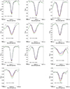 |
Fig. 1. Example of the synthesised lines for one star of our sample (NGC 2808−49743). The red line represents the best fit. Blue and green fits correspond to the best fit of each element ±0.1 dex, respectively. |
Abundances obtained for each element analysed in each GCs.
5. Observational uncertainties
The uncertainty associated with the measurements combines the uncertainties of the best-fit determination and those associated with the uncertainties in the adopted atmospheric parameters. As we are adopting parameters from C09 and Carretta et al. (2017), we are also adopting the errors associated with the atmospheric parameters described there. It is worth noticing that, for the species analysed in C09 and Carretta et al. (2017), the error associated with log g and [Fe/H] have generally a quite limited influence on the budget of the total error. Heavy elements, whose abundances are generally measured from transitions of ionised species, are more sensitive to log g variations.
Because this sample is meant to be compared to different GCs, the observational uncertainties should consider both the individual star-to-star errors (arising from e.g. stochastic uncertainties in the photometry associated with the line-to-line scatter, etc.) and the cluster systematic error associated with overall cluster characteristics (e.g. overall reddening). A full table with the errors computed by C09 can be found in their Table 7.
5.1. Individual star error
To determine the individual star errors, we followed the approach described by Schiappacasse-Ulloa & Lucatello (2023, hereafter SUL23). That error is associated with the abundance determinations and combines both the uncertainties of the best-fit determination and the uncertainties in the assumed stellar parameters. For abundances derived via synthesis, the first one comes from the error on the best-fit determination (e.g. the continuum position). The second is derived by evaluating the variation of the abundances to the change in each of the parameters (Teff, log g, vt, and [Fe/H]), keeping fixed the remaining ones. We selected one star of each cluster as a representative, trying to use the one with median stellar parameters. The variations in stellar parameters assumed to compute the sensitivity matrix (Table 3) are: ΔTeff = 50 K, Δlog g = 0.2 dex, Δvt = 0.1 km s−1, and Δ[Fe/H] = 0.1 dex. The final estimated error (σ) derived from the variation of stellar parameters is listed in Table 4. Moreover, we listed the rms error defined as the standard deviation divided by the squared root of the stars with actual measurements minus one.
Element sensitivity to the parameter variations (ΔTeff = +50 K, Δlog g = +0.2 dex, Δ[Fe/H] = +0.10, and Δvt = +0.10).
5.2. Cluster systematic error
The error coupled to Teff comes from the empirical relation between Teff and the (V − K) colour given by Alonso et al. (1999). Since the V − K are dereddened, C09 and Carretta et al. (2017) estimated the error from the reddening adopted, affecting their Teff values. To get the internal error of the log g, they propagated the uncertainties in distance modulus, the star’s mass, and the error associated with Teff. The one associated with vt is given by its internal error divided by the square root of the star number. Finally, the error coupled to the metallicity was given by the quadratic sum of the systematic error contribution of the systematic contribution Teff, log g, and vt multiplied by their correspondent abundance sensitivity. The last term was given by the rms scatter in a given element divided by the square root of the star number of a given cluster.
5.3. Data interpretation
To determine the strength of a given relationship between two abundances, we used the so-called “Spearman coefficient”, also known as the “Spearman rank” (Spearman 1904). To characterise a correlation, we considered p-values lower (higher) than 0.01 (0.05) as highly (poorly) significant. Moreover, a p-value between 0.01 and 0.05 is considered mildly significant. The Spearman rank and its p-value will be indicated when corresponding along the text and figures. In addition, we quantified the variation of any correlation in the present article by simply using the slope of a one-degree fit to the two elements considered.
6. Chemical abundance distribution: Cu
6.1. Internal spread
Only a handful of studies (e.g. Cunha et al. 2002; Simmerer et al. 2003) have analysed the presence of copper in GCs. However, they found no evidence of internal variation. As Cu abundances are derived from relatively strong lines, we tested whether there is any dependency of the derived values on vt. In the more metal-poor clusters, the Cu abundances are dominated by upper limits. Figure 2 displays the behaviour of Cu with respect to vt, (ordered by increasing metallicity7) showing no clear trend, except for NGC 6121, which has a positive correlation highly significant. We note that we use the Cu abundance obtained by re-scaling to the mean Cu within each cluster to better visualise the sample. In most cases, the Cu results seem to be (within the errors) quite flat and without spread. However, the most metal-rich GCs (NGC 6171, NGC 6838, and NGC 104) display a spread larger than the associated error. On the other hand, the GC NGC 6254 has two stars with slightly higher Cu abundances, considering the associated errors.
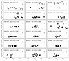 |
Fig. 2. Δ(Cu)MEAN along with vt for each GC of the sample. The respective Spearman corr. and p-values are indicated on each panel. Filled circles and empty triangles represent actual Cu measurements and upper limits, respectively. |
To further analyse whether this discrepancy is real, we show in Fig. 3 a comparison of two stars with similar stellar parameters to those of GC NGC 6171. The difference in A(Cu) is about 0.75 dex, which goes beyond the associated errors but is consistent with the difference observed in the lines and cannot be explained by the slight difference in vt. It is worth noticing that the Cu enrichment goes in the opposite direction of the n-capture enrichment for the pair. This may suggest that in this pair, the nucleosynthesis process(s) responsible for the n-capture production is (are) not linked to the one responsible for the Cu production. Some authors (e.g. Pignatari et al. 2010) have claimed that it may be related to the s-process production in massive stars or AGB stars, which is investigated later in this paper.
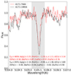 |
Fig. 3. Pair of stars of the GC NGC 6171 with similar stellar parameters as reported by Carretta et al. (2009), a different Cu abundance. Black and red lines represent the spectra of ID = 19956 and ID = 7948, respectively. |
In this context, it is interesting to consider the Cu relationship with Na. In Fig. 4, we show the distribution of Cu abundances as a function of the ΔNa content in each cluster. This value has been used to eliminate any possible spurious dependencies of abundances from the adopted vt, an effect that impacts the elemental abundances derived from strong lines.Thus, Δs measurements were defined as follows: for a given element X, Δ(X) is defined as the difference between the reported [X/Fe] abundance, and a linear fit between the [X/Fe] and vt. The distribution seems to be quite flat along with Na, meaning that there is no obvious link in the production between these two species. The only exceptions are GCs NGC 6218 and NGC 5904, with significantly high Spearman correlations.
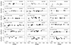 |
Fig. 4. [Cu/Fe] distribution along with Δ(Na) for each GC analysed. The respective average and standard deviation Cu abundance are indicated in solid and dashed lines, respectively. Symbols follow the same description as in Fig. 2. |
6.2. Cu overall distribution
Figure 5 shows the Cu distribution along the [Fe/H] in the Galactic field and GCs. In the present figure, grey crosses represent the Cu abundances for mostly halo field stars (with a handful from the thick disk) reported by Ishigaki et al. (2013). In addition, we complement our results with GC abundances from the literature when possible: NGC 1851 (Carretta et al. 2011), NGC 362 (Carretta et al. 2013), Terzan 8 (Carretta et al. 2014a), NGC 4833 (Carretta et al. 2014b), and NGC 6093 (Carretta et al. 2015), all of them represented with red-filled crosses. It is worth noticing that the literature GCs were analysed using analogous techniques (stellar parameter determination and abundance analysis). The colours were assigned to each solid symbol to represent the different GCs present in this sample. We linked the GCs in common with Simmerer et al. (2003) with a dashed line for an easy comparison. GCs display a steep increase for metallicities higher than −2.0 dex, however, most GCs closely follow the field star distribution, indicating that they do not experience a particular Cu enrichment.
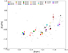 |
Fig. 5. [Cu/Fe] distribution along the [Fe/H] for the whole sample. The analysed GCs are shown with coloured squares. Grey crosses show the field star abundances from Ishigaki et al. (2013). Red-filled crosses display the reported abundance of Cu in different GCs in the literature. Black circles represent results reported by Simmerer et al. (2003) for our in-common GCs (linked with a black dashed line). |
Simmerer et al. (2003) analysed Cu abundance in a large sample of GC using the Cu lines at 5105 Å and 5787 Å. It is worth noticing that the latter line is a better Cu indicator, which is neither saturated nor crowded by other species. Unfortunately, the mentioned line is located in the gap of the spectra analysed here. While there is good agreement among in-common GCs with lower metallicity (NGC 6254 and NGC 7078), for the GCs with higher metallicities (NGC 6121, NGC 5904, and NGC 288), the cited article reported considerably lower (except for NGC 6838) Cu abundances (with differences ranging from 0.05 to 0.50 dex) than the ones reported in the present article.
This discrepancy can be partially explained by the difference in the metallicity adopted, meaning that a model atmosphere with high metallicity reproduces a stronger Cu line than a model with a lower one. In addition, the sensitivity of the line at 5105 Å to the change in vt, plus the presence of MgH lines in the more metal-rich regime, could also play a role in this difference. For the stars with these problems, Simmerer et al. (2003) determined the Cu abundance using the line at 5787 Å. Although we have stars in common with Simmerer et al. (2003), there is only one for which they determined the abundance from the line at 5105 Å. For those stars, the stellar parameters used in both (ours and theirs) analyses are practically the same and the amount of Cu obtained is −0.27 ± 0.10 and −0.30 ± 0.10 dex, respectively. In particular, the large spread found in the present article for NGC 6254 was also reported by Simmerer et al. (2003). On the other hand, they also reported a particularly high Cu content in NGC 6121 compared with other GCs with similar metallicities. NGC 2808 has similar metallicity as NGC 6121, but they display quite different Cu content in our analysis. Given that there is a pair of stars with similar parameters, one in each of the two clusters, it is possible to assess the existence of such a difference directly. Figure 6 shows such a comparison for the Cu line. The figure reinforces that the difference is real and is not due to any dependency on stellar parameters. In the case of NGC 6171, the trend with vt does not seem to be present, but it displays a particular Cu enrichment.
 |
Fig. 6. Pair of stars of the GCs NGC 2808 (ID = 8739; red line) and NGC 6121 (ID = 27448; black line) with similar stellar parameters and different Cu abundance. |
7. Chemical abundance distributions: Y, Ba, La, and Eu
7.1. Ba-Y dependency with vt
Based on three rather strong lines, Ba abundances show considerable sensitivity to the adopted vt. This is a common finding in cool giants, as discussed, for instance, by Worley et al. (2013). It is worth noticing that the sensitivity of these species to vt is independent of the method used for the vt derivation. We explored averaging Ba abundances weighted by their respective errors using the different combinations of lines to minimise this effect and concluded that the best combination is, indeed, the use of all three available to us. Hereinafter, we opted to use all three lines for our final abundance due to the reduction of both the spread and the lessening of the vt dependence. Similar considerations apply to the Y II lines used to derive [Y/Fe]II abundances.
In addition, we computed ΔX for Y and Ba to get rid of the trend given by vt in the whole sample. Figure 7 shows an illustrative example for the GC NGC 1904. A strong negative Spearman correlation (about −0.80) is clearly shown in the left panel of both figures. The right panels show how the trend is avoided by using the Δs (defined in Sect. 6).
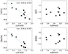 |
Fig. 7. [Y/Fe] ([Ba/Fe]) abundances and Δ(Y) (Δ(Ba)), respectively, as a function of vt for the GC NGC 1904, shown in the upper (lower) left and right panels. The blue dotted line shows the linear fit. |
7.2. Internal n-capture spread
For the sake of this section, we remind the reader of the effects of vt on Y and Ba (discussed in Sect. 4). Because of this effect, in general, the larger the range covered by vt, the larger the dispersion driven by this parameter.
As can be seen from Table 5, the GCs NGC 6171 ([Fe/H] = −1.03 dex) and NGC 7078 ([Fe/H] = −2.32 dex) display both a large rms error and IQR in Y and Ba. The Ba dispersion plus the constant Y found in NGC 7078 is in good agreement with previous results in the literature, where NGC 7078 has been reported as an r-process enriched cluster by several literature sources (e.g. Kirby et al. 2020). At the cluster metallicity, Ba is mostly produced by the r-process. On the other hand, NGC 6171 shows a large spread in all the elements analysed in the present article. This mildly significant spread agrees with O’Connell et al. (2011), who speculated about a potential early r-process enrichment in the cluster due to the evidence of La and Eu spread. However, because of the small number of stars it is based on, this spread should be taken with caution.
7.3. Non-LTE correction for Y
Because our sample spans a large range of stellar parameters, non-LTE correction is a factor to take into consideration, especially due to their strong dependency on metallicity, which could lead to unreal abundance trends in our results. Storm & Bergemann (2023) presented the Y non-LTE correction for a large range of stellar parameters in different Y lines. For the stars in our sample, the corrections range from ∼0.05 and ∼0.15 dex. Then, in the worst-case scenario, the maximum variation would be around 0.10 dex, which has a limited impact on the current analysis. Moreover, Guiglion et al. (2024) showed the Y spread along with the [Fe/H]; the results reveal that the spread did not change considerably (∼0.02 dex), meaning that non-LTE corrections would not modify the potential spreads within a given cluster. Similar results were reported for Ba in the same article. Therefore, our results do not consider non-LTE corrections.
7.4. Comparison with the literature
D’Orazi et al. (2010) analysed the Ba abundances of 15 GCs included in our sample, for which we have 55 stars in common; however, using lower resolution GIRAFFE spectra of a larger number of stars per cluster. They used equivalent width to determine the chemical abundances and adopted stellar parameters derived identically from those used in the present article. Because the Ba abundances for individual stars were not published, Fig. 8 shows the comparison of our and their average Ba abundance for the 15 in-common GCs. We got constantly lower abundances for the whole sample. As shown in the figure, the average difference between our and their results is ![Mathematical equation: $ \overline{\delta\mathrm{[Ba/Fe]}} $](/articles/aa/full_html/2024/05/aa48805-23/aa48805-23-eq1.gif) = −0.12 ± 0.12 dex, probably due to the different methods used in the abundance determination and the lines considered. While we used Ba lines at 5853 Å, 6141 Å, and 6496 Å, D’Orazi et al. (2010) used only the second one.
= −0.12 ± 0.12 dex, probably due to the different methods used in the abundance determination and the lines considered. While we used Ba lines at 5853 Å, 6141 Å, and 6496 Å, D’Orazi et al. (2010) used only the second one.
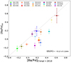 |
Fig. 8. Comparison of Ba abundances obtained in the present article with D’Orazi et al. (2010) for in-common GCs. The average difference between our and their results, |
![Mathematical equation: $ \overline{\delta\mathrm{[Ba/Fe]}} $](/articles/aa/full_html/2024/05/aa48805-23/aa48805-23-eq2.gif)
7.5. The n-process elements: Relation with O, Na, and Mg
With a few exceptions, GCs have not shown heavy element variations among their different populations and are not involved in the MSP phenomenon. Similarly to the analysis done by SUL23 for NGC 6752, we explored the variation of ΔY and ΔBa with respect to Na. Figures A.1–A.3 show the results for the Y and Ba abundances as a function of the O, Na, and Mg, respectively, for each cluster of the sample. The Spearman correlation for actual measurements is reported in each panel. In the first figure, only weak or poorly significant correlations exist between Y and O in the whole sample. A few clusters (NGC 7078 and NGC 6121) show a negative correlation between Ba and O highly significant, which could be translated in a Ba decrease of about 0.07 and 0.05 dex for each 0.10 dex increment of O, respectively. In the second figure, the results for Y and Ba seem to display quite constant abundances within the associated errors along the different Na. However, there are GCs such as NGC 2808, NGC 6397, and NGC 3201 that display a positive correlation highly significant between Y and Na, which would produce an increment in Y of about 0.03, 0.015, and 0.02 dex for each increment in Na of 0.1 dex, respectively. Finally, the last figure shows the relation of Y–Mg and Ba–Mg. Most of the clusters display weak or non-significant Y–Mg correlations. The exception of it are the GCs NGC 1904, NGC 6121, and NGC 2808. Interestingly, the two latter clusters have a negative correlation, whereas the first has a positive one. In particular, NGC 1904 would have a Y increment of 0.06 dex for each 0.10 dex Mg, whereas NGC 6121 and NGC 2808 show a Y decrease of 0.17 and 0.03 dex for a Mg increment of 0.10 dex, respectively. Concerning the relation Ba–Mg, the GCs NGC 1904, NGC 3201, and NGC 2808 display a strong correlation, with the last GC the only one with a negative relation. While the latter displayed a Ba decrease of about 0.03 dex for each Mg increment of 0.10 dex, NGC 1904 and NGC 3201 showed an increment of 0.09 and 0.16 dex. Nevertheless, having s-process elements correlating with Na, without a corresponding negative correlation with Mg (or vice-versa) could indicate spurious occurrences due to the small number of statistics. On the other hand, because the proton-capture reactions produce intrinsically small Mg depletion (as opposed to large enhancements in Na), the Mg variations are difficult to observe. Then, these results should be taken with caution.
Similarly, Fig. A.4 shows the results for La and Eu along with Δ(Na). Although La and Eu abundances are dominated by upper limits in the more metal-poor clusters, the distribution of La and Eu does not display considerable spread. The only exceptions are the GCs NGC 7078 and NGC 6171, which display a larger Eu spread supporting the scenario of the r-process enrichment mentioned previously. Moreover (in most clusters), the La and Eu results display a constant abundance along Na, demonstrating the lack of correlation between these species. However, NGC 6121 showed a mildly significant correlation between La and Na. Similar results were found for NGC 3201, NGC 288, and NGC 6752 for Eu and Na.
The trends were then examined on the combined sample, that is to say, on all the stars analysed in the present work, separated into groups according to their overall metallicity. To do so, Figs. 9–11 show the Δ(Y) (upper row) and Δ(Ba) (lower row) as a function of Δ(O), Δ(Na), and Δ(Mg), respectively. This exercise aims to probe the variation of s-process elements along with the O, Na, and Mg abundance. Therefore, NGC 7078, known to display n-capture element spread attributable to the r-process, was excluded from the combined sample. The panels display the distribution for three metallicity bins: [Fe/H] < −1.80 dex (metal-poor; left panels), −1.80 dex < [Fe/H] < −1.10 dex (metal-mid; mid-panels), and [Fe/H] > −1.10 dex (metal-rich; right panels). Each figure indicates the corresponding Spearman coefficient and p-value for each metallicity bin. All the panels show quite flat distributions and weak correlations, which is valid for the whole sample and each metallicity bin.
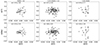 |
Fig. 9. ΔY (upper panels) and ΔBa (lower panels) as a function of ΔO for the whole survey sample (except for NGC 7078). The sample was divided into three metallicity bins: [Fe/H] < −1.80 dex (metal-poor; left panels), −1.80 dex < [Fe/H] < −1.10 dex (metal-mid; mid-panels), and [Fe/H] > −1.10 dex (metal-rich; right panels). The respective Spearman coefficient and p-value are reported on each panel. |
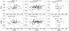 |
Fig. 10. ΔY (upper panels) and ΔBa (lower panels) as a function of ΔNa. It follows the same description as Fig. 9. |
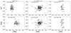 |
Fig. 11. ΔY (upper panels) and ΔBa (lower panels) as a function of ΔMg. It follows the same description as Fig. 9. |
However, it is worth noticing that for the mid-metallicity regime (mid-panels), there is a mildly significant correlation between Y and Na. The correlation is similar in the low metallicity bin; however, its significance is lower than in the mid-metallicity regime and, in the high one, it disappears entirely. We note, however, that in case of an actual correlation between those abundances, such a metallicity regime should be the most suitable one to detect it. In fact, in this regime, the lines are strong enough to be scarcely affected by noise but weak enough to have to be weakly affected by the vt so that a linear fit can appropriately address its contribution. This correlation in the mid-metallicity regime would be translated in a Y increment of about 0.01 dex for each 0.1 dex increment of Na.
7.6. Heavy element distributions
With an aim to take a look at the overall content in n-capture elements, a comparison of the heavy elements analysed for the sample of GCs and the galactic field was performed. In Fig. 12, we show (from top to the bottom) the results obtained for [Y/Fe], [Ba/Fe], [La/Fe], and [Eu/Fe], along with the [Fe/H]. The field star distribution (grey crosses) was taken from SAGA Database8 Suda et al. (2008). Each GC is represented with a different colour. Squares and triangles are actual measurements and upper limits, respectively. As done in Fig. 5, we included (when available) the literature results (in red crosses) from Carretta et al. (2011) (NGC 1851), Carretta et al. (2013) (NGC 362), Carretta et al. (2014a) (Terzan 8), Carretta et al. (2014b) (NGC 4833), and Carretta et al. (2015) (NGC 6093). In addition, Table 4 displays the mean, spread, and the number of stars used to get the actual abundance for each element.
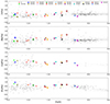 |
Fig. 12. [Y/Fe], [Ba/Fe], [La/Fe], and [Eu/Fe] as a function of the [Fe/H] for the whole sample, shown from top to bottom. Coloured squares represent the GCs analysed in the present sample. Red-filled crosses represent GCs abundance from the literature as in Fig. 5. Grey dots show the field star abundances, and grey crosses represent bonafide Halo field stars ([Mg/Fe] > 0.2 dex) taken from the SAGA database (Suda et al. 2008). |
Field stars show a yttrium distribution that increases with the metallicity having Y abundances ranging from ∼−0.60 dex at low metallicities up to solar abundances at high metallicities. In the upper panel, most of the GCs analysed follow closely the trend displayed by field stars at the correspondent metallicity. We see that NGC 6121 and NGC 6171 are the only exceptions, displaying larger Y abundances than the field star counterparts.
Barium, at solar metallicity, mainly reveals an s-process origin (85%; Sneden et al. 2008): Ba shows similar behaviour to Y along with [Fe/H]; however, the former displays slightly lower abundances than Y at [Fe/H] < −1.5 dex. In the second panel, similar to Y results, Ba abundances in almost all the GCs analysed follow the field stars trend. The GCs NGC 6121, NGC 6171, and NGC 7078 display higher abundance than expected for stars at that metallicity.
Field stars display a lanthanum distribution slightly super-solar at [Fe/H] < −1 dex, which becomes solar for richer metallicities. The third panel shows that the GCs surveyed fit the field stars trend. It is worth noticing that only the upper limit was set for the metal-poor GCs NGC 7099, NGC 4590, and NGC 6397 because the La lines became too weak. For NGC 7078, La abundance was determined in only one star, so the result should be taken cautiously.
Europium is known to be a pure r-process element (97% at solar metallicity; Simmerer et al. 2004). In the lowest panel, the Eu distribution in the field displays a quite constant over-abundant at about [Fe/H] < −0.7 dex, which constantly decreases toward higher metallicities, showing the iron production by SN Ia after 0.1−1.0 Gyr, which agrees with both observations and models (Cescutti et al. 2006). All the GCs analysed seem to follow closely the upper envelope of the distribution drawn by the field stars. It is worth noticing, that in the GCs NGC 4590 and NGC 7099, the Eu detection was not possible. Moreover, the GC NGC 7078 displays a slight Eu over-abundance with respect to the field stars at the same metallicity.
In general, most of the surveyed GCs closely follow the field distribution9, meaning there is no evidence of a peculiar n-capture enrichment. Our results are in good agreement with literature GCs of similar metallicity.
On the other hand, Table 5 reports the IQRs of [Y/Fe], [Ba/Fe], [La/Fe], and [Eu/Fe]. Upper limits were not considered in the IQR computation for La and Eu. It is worth noticing that off-trend GCs display (NGC 7078, NGC 6171, and NGC 6121) also a larger internal dispersion. NGC 7078 has been reported as a GC with the largest spread in both Ba and Eu. The present analysis reports a [Ba/Fe] abundance ranging from −0.29 dex to 1.02 dex. Previous studies have reported a difference of ∼0.45 dex (Otsuki et al. 2006) and ∼0.55 dex (Sobeck et al. 2011). The larger Ba spread found in the present analysis can be related to the larger vt range compared to the cited articles. For comparison, when the Ba intrinsic spread (without considering the effect of vt) is considered, it decreases to ∼0.80 dex. In a larger sample of 63 stars, Worley et al. (2013) reported bimodal distribution for both Ba and Eu, finding a difference of up to 1.25 dex for the first one and about 0.80 dex for the second one. In the case of the present article, the [Eu/Fe] difference is at least 0.59 dex (upper limits could enlarge this difference), which is similar to the difference reported by Otsuki et al. (2006) (∼0.55 dex) and Sobeck et al. (2011) (0.57 dex) in their sample of three RGB stars. The large dispersion reported in both Ba and Eu, presented in our results and the literature, agrees with a peculiar r-process element enrichment.
Observational and rms error (excluding the vt contribution) for each cluster.
On the other hand, NGC 6171 displays a large IQR in all the n-capture elements measured. O’Connell et al. (2011) analysed the La and Eu abundances in 13 stars of the cluster, which showed a good agreement with the present article (⟨[La/Fe]⟩ = 0.41 ± 0.12 and ⟨[Eu/Fe]⟩ = 0.73 ± 0.13). Moreover, they reported a large difference in the Eu (∼0.50) and La (∼0.40) content in their sample, which agrees with the large IQR mentioned before arguing in favour of an early r-process enrichment. Finally, the GC NGC 6121 was found to show a Y bimodal distribution (Villanova & Geisler 2011), which was later challenged by D’Orazi et al. (2013), whose results are consistent with the present analysis. The cluster was found to display an intrinsic high s-process enrichment due to a particular higher concentration of these species in the protocluster cloud (Yong et al. 2008), which agrees with the [Y/Fe] = 0.44 dex and [Ba/Fe] = 0.50 dex found by D’Orazi et al. (2013, 2010), respectively. Moreover, the La (0.48 dex) and Eu (0.40 dex) results from Yong et al. (2008) are in good agreement with the ones presented here. Further discussion of internal spread is beyond the aims of the present paper and will be addressed in an upcoming work, currently in preparation.
7.7. [Ba/Eu] and [Ba/Y] ratios
Figure 13 shows the ratio between the Ba and Y (right panel) and Ba over Eu (left panel) as a function of [Fe/H]. The ratio of these elements can provide means to disentangle the contribution of the r- and s-process to the heavy element content in the cluster. The symbols follow the same arrangement as the previous figures. In addition, on the right-hand panel, we included in magenta diamonds dwarf galaxies results from Suda et al. (2008) to compare their behaviour and the one for GCs.
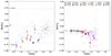 |
Fig. 13. Abundance ratios of [Ba/Eu] and [Ba/Y]s as a function of [Fe/H], respectively, shown in the left and right panels. Dashed lines at [Ba/Eu] 0.70 dex and −0.70 dex indicate the ratio for a full s-process and full r-process enrichment. The dashed line at [Ba/Eu] 0.00 dex displays the solar ratio. Magenta diamonds in the right-hand panel show dwarf galaxies results taken from Suda et al. (2008). Other symbols and colours follow the description given in Fig. 12. |
The [Ba/Eu] distribution as a function of [Fe/H] provides insight into the process by which our Galaxy was enriched. The dotted horizontal lines at [Ba/Eu] −0.70 dex and 0.70 dex, reflect a pure enrichment from r-process and s-process species, respectively. The [Ba/Eu] pattern followed by the field stars goes from a pure r-process enrichment at low metallicities to a continuous contribution of s-process at solar metallicity. Although there are GCs with similar metallicities but discrepant [Ba/Eu] (e.g. NGC 2808 and NGC 6121), the results for most of the GCs display a similar behaviour as field stars. In addition, if [Fe/H] is considered a proxy of time (with more metal-poor stars being older than the ones with higher metallicity) it is possible to see the rise of the s-process elements along the time. The results are compatible with pure r-process abundances for the more metal-poor cluster, meaning that their abundances are influenced by explosive events, such as SNe type II or merging neutron stars. As field stars, in GCs, the contribution of the s-process enrichment increases with metallicity; however, it remains dominated by the r-process. It is worth noticing that for the GCs NGC 4590 and NGC 7099, we reported lower limits for the [Ba/Eu] ratios.
In s-process production, Y and Ba are part of the first and second peaks of s-process elements, respectively. Consequently, their ratio investigates the contribution of ls and hs elements. In the case of AGB stars, their nucleosynthesis is linked to the stars’ mass and metallicity. Specifically, the [hs/ls] ratio tends to decrease as the star mass increases, which can vary depending on the star’s metallicity. Nevertheless, when dealing with low metallicities, such as those observed in metal-poor globular clusters (GCs), the r-process contributes to the synthesis of Ba and Y. This complicates the direct use of the [Ba/Y] ratio in this scenario. To address the r-process contribution of these elements, we adopted values for the r-process contribution to Ba and Y from the solar system r-pattern derived by Simmerer et al. (2004). These values are scaled to align with the europium (Eu) abundance measured in both GC and field stars. The notation [Ba/Y]s denotes the Ba over Y ratio, considering only the contribution from the s-process. The results are shown in the right panel of Fig. 13, which reveals that the [Ba/Y]s ratio in the GC sample remains constant at low metallicity, but decreases at metallicities higher than −1.5 dex. The decrement is also seen in a fraction of field and dwarf galaxy stars; however, the behaviour of GCs regarding the [Ba/Y]s ratio seems better defined. The increase [Fe/H] prompts a shift in the s-process pattern of GC towards Y instead of Ba. This shift, from the hs to the ls elements, suggests an augmented contribution from lower-mass AGB stars at later stages of MW evolution.
7.8. Cluster comparisons: Cluster-to-cluster differences
To assess the discrepant Ba/Eu ratios among GCs with similar metallicities, we compared pairs of stars with similar stellar parameters in different clusters. The comparison is shown in Fig. 14. The pairs also share similar Na abundances to those reported by Carretta et al. (2009). In the first row of the figure, the comparison between the stars of NGC 6121 (ID = 27448) and NGC 2808 (ID = 8739), two clusters with similar metallicities ([Fe/H] ∼ −1.2 dex), but quite different n-capture abundance. As the spectra comparison shows, there is higher abundance in their s-process elements (Y, Ba and La); however, this behaviour changes for the r-process elements. Because the stars have only slightly different vt values, its effect cannot explain such a difference in abundance. This comparison suggests that the large difference(∼0.70 dex) shown in Fig. 13 is real, meaning the NGC 6121 has a higher enrichment of s-process elements than NGC 2808 and the latter has a higher r-process enrichment. The second row compares a star pair, in GCs NGC 3201 (ID = 541657) and NGC 5904 (ID = 900129). The two stars with similar stellar parameters and Na abundance show a systematic overabundance in favour of the second one for all the elements analysed, suggesting an overall different n-capture enrichment, but still slightly more shifted to the r-process.
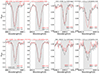 |
Fig. 14. Pair of stars with similar stellar parameters and Na abundances as was reported by Carretta et al. (2009), but different n-capture abundances. From left to right: Y line at 4883 Å, Ba line at 5853 Å, La line at 6391 Å, and Eu line at 6645 Å. |
7.9. Comparison with chemical evolution models
As mentioned in Sect. 1, the main nucleosynthetic sites for the s- and r-processes are mainly AGB stars (with some contribution of FRMS) and neutron star mergers and magneto-rotational driven (MRD) SNe, respectively. Cescutti & Chiappini (2014) proposed a model for the chemical enrichment of the halo considering different sources of heavy elements (for details on the model, we refer to the cited article). In particular, they tested the models with electron capture (EC) SNe and/or MRD SNe with and without an early enrichment of s-process elements from FRMS. According to Cescutti & Chiappini (2014), to better reproduce the observed n-capture element distribution in the Galactic halo, the model should take into account a mix of pollution coming from FRMS and MRD for the s- and r-process enrichment, respectively. Figure 15 shows the comparison of our results (coloured symbols) and the predictions for Y, Ba, La, and Eu from the aforementioned model. The figure is coloured by logstars, which reflects the probability of finding a long-living star. As shown in the present figure, the model closely reproduces the observations except for the [Y/Fe] and [Ba/Fe] abundances in NGC 6121 and NGC 6171, which (as discussed previously) show a particularly high content in these elements. In addition, although those clusters show a La abundance in good agreement with the models, it is worth noticing that they are located in the upper envelope of the model’s distribution.
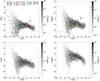 |
Fig. 15. Comparison between the n-capture element abundances measured in the present work and modelled abundances from Cescutti & Chiappini (2014) coloured-coded by the logarithmic number of stars in each bin. |
As commented by Cescutti & Chiappini (2014), both r-process sources analysed in their models (EC SNe and MRD) reproduce the halo distribution of Eu quite well, displaying a good agreement among these sources in the most metal-poor regime ([Fe/H] < −2 dex), albeit with some slight discrepancies at intermediate metallicities (−2 dex < [Fe/H] < −1 dex). The model used in comparison with our results reflects good agreement with the metallicity of our sample being no discrepant with the MRD + FRMS scenario. We hope that in the future, with current and subsequent observational constraints, we could shed light on the contributor sources of n-capture elements of the halo.
8. In situ and ex situ GCs
Various authors have attempted to determine the origin of GCs and relate it to both their dynamical and chemical features. We used the results published by Massari et al. (2019) to identify potential relations with the n-capture element abundances obtained in the present article. Among the GCs in our sample, there are 16 previously analysed by Massari et al. (2019), of which: 7 were identified as in situ (NGC 104, NGC 6171, NGC 6218, NGC 6397, NGC 6752, NGC 6838, and NGC 7078), 6 as ex situ (NGC 288, NGC 2808, NGC 3201, NGC 4590, NGC 5904, and NGC 7099) and which happen to be closely associated with the Gaia-Enceladus Stream, and 3 GCs of uncertain origins (NGC 6121, NGC 6809, and NGC 6254).
We analysed whether in situ and ex situ GCs behave differently. We found that all the GCs identified as “in situ” showed slightly higher Y and Ba abundances with respect to the ex-situ GCs; moreover, the latter displayed smaller spreads than the first ones in all the n-capture analyses. The mean and standard deviation for in situ (ex situ) GCs are ![Mathematical equation: $ \overline{\mathrm{[Y/Fe]}} $](/articles/aa/full_html/2024/05/aa48805-23/aa48805-23-eq3.gif) = −0.07 and σ([Y/Fe]) = 0.21 (
= −0.07 and σ([Y/Fe]) = 0.21 (![Mathematical equation: $ \overline{\mathrm{[Y/Fe]}} $](/articles/aa/full_html/2024/05/aa48805-23/aa48805-23-eq4.gif) = −0.15 and σ([Y/Fe]) = 0.16),
= −0.15 and σ([Y/Fe]) = 0.16), ![Mathematical equation: $ \overline{\mathrm{[Ba/Fe]}} $](/articles/aa/full_html/2024/05/aa48805-23/aa48805-23-eq5.gif) = 0.09 and σ([Ba/Fe]) = 0.24 (
= 0.09 and σ([Ba/Fe]) = 0.24 (![Mathematical equation: $ \overline{\mathrm{[Ba/Fe]}} $](/articles/aa/full_html/2024/05/aa48805-23/aa48805-23-eq6.gif) = -0.02 and σ([Ba/Fe]) = 0.16),
= -0.02 and σ([Ba/Fe]) = 0.16), ![Mathematical equation: $ \overline{\mathrm{[La/Fe]}} $](/articles/aa/full_html/2024/05/aa48805-23/aa48805-23-eq7.gif) = 0.20 and σ([La/Fe]) = 0.17 (
= 0.20 and σ([La/Fe]) = 0.17 (![Mathematical equation: $ \overline{\mathrm{[La/Fe]}} $](/articles/aa/full_html/2024/05/aa48805-23/aa48805-23-eq8.gif) = 0.20 and σ([La/Fe]) = 0.13), and
= 0.20 and σ([La/Fe]) = 0.13), and ![Mathematical equation: $ \overline{\mathrm{[Eu/Fe]}} $](/articles/aa/full_html/2024/05/aa48805-23/aa48805-23-eq9.gif) = 0.56 and σ([Eu/Fe]) = 0.18 (
= 0.56 and σ([Eu/Fe]) = 0.18 (![Mathematical equation: $ \overline{\mathrm{[Eu/Fe]}} $](/articles/aa/full_html/2024/05/aa48805-23/aa48805-23-eq10.gif) = 0.56 and σ([Eu/Fe]) = 0.12) dex. We note that GCs with upper limits were not considered in that calculation.
= 0.56 and σ([Eu/Fe]) = 0.12) dex. We note that GCs with upper limits were not considered in that calculation.
Firstly, we investigated whether these slight discrepancies in the average abundances were linked to differences in metallicity, age, or vt. We found that for Ba and Y, there seems to be a trend with metallicity, as the most metal-rich ones have systematically higher abundances of these elements. As each cluster spans approximately the same evolutionary range, the Ba and Y transitions in metal-rich clusters are more likely to be saturated, and the measurement of abundances from them might be affected by systematic errors. Nevertheless, it is worth noticing that this effect would not affect the internal spread of each cluster and (in any case) the overall pattern as a function of metallicity is in good agreement with the field. Secondly, because s-process production changes over time, we investigated any potential relation with the cluster age. To this aim, we used the results determined by VandenBerg et al. (2013); however, there were no trends seen for GCs with different origins. Finally, after analysing the maximum difference of vt within each cluster, we note that this difference seems quite homogeneous along the clusters (with only two outliers), meaning that vt affects all these clusters similarly. Thus, this behaviour is not caused by different ranges in vt. Nevertheless, a Student’s t-test comparing the mean abundances of these two groups showed that their differences were not significant. Therefore, there is no evidence of different chemical evolution among them.
9. Chemical abundances and cluster mass
Several studies have compared the abundance patterns of GCs with global properties such as cluster mass. Using part of the sample presented here, Carretta et al. (2009) related the Mg-Al anti-correlation with the mass and the metallicity of the GCs, which was later confirmed by Pancino et al. (2017). Similarly, Masseron et al. (2019) analysed a sample of 885 GC stars and found evidence of a correlation of the Al spread present in GCs with the cluster mass. The latter suggested that the Mg-Al reaction decreases its importance in more massive GCs. It is interesting to perform a similar analysis using the n-capture element abundances. A comparison was performed against the absolute magnitude (MV), a proxy for the cluster mass. The relation between MV (from Harris catalogue; Harris 2010) and the spread reported (represented by the IQR) for Y, Ba, La, and Eu can be seen in Fig. 16. All the mentioned IQRs display a quite flat distribution with a quite constant spread along the MV, meaning there is no evidence of any trends with cluster mass neither in s-process species nor Eu abundances. Hence, we find no evidence that cluster mass does play a role in retaining n-capture-enriched material.
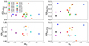 |
Fig. 16. IQRs for Y, Ba, La, and Eu abundances as a function of the absolute visual magnitude for the whole sample. The MV values were taken from the Harris catalogue (Harris 2010). |
10. Discussion
In general terms, insofar as heavy elements are concerned, the GCs in our sample behave similarly to field stars at the same metallicity. Nevertheless, some present peculiarities, such as significant spreads or correlations between elements. Those cases are briefly discussed below.
NGC 7078. It displays considerable n-capture element dispersion, explained by peculiar chemical enrichment from an r-process. Moreover, we found highly significant correlations between Ba and O and Na, being negative and positive, respectively. These correlations suggest that the nucleosynthetic sites destroying (producing) O (Na) were also contributing to the Ba production.
NGC 1904. Although it has shown quite similar behaviour to field stars at its metallicity, NGC 1904 displays a significant correlation between both Y and Ba with Mg. The dispersion in all these elements is modest, however, the nucleosynthetic site responsible for the little Mg destruction would also deplete a small amount of s-process elements.
NGC 2808. It shows a quite constant n-capture distribution, however, correlating with Na. In addition, it presents a negative correlation (highly significant) correlation between both Y and Ba with Mg. According to C09, NGC 2808 presents a large dispersion in Mg (up to 0.7 dex), which seems to be bimodal. Because the Mg-poor group has higher abundances of Y and Ba, the responsible for the Mg production in NGC 2808 should be able to destroy s-process species. This highlights the fact that a positive correlation between Y and Na, coupled with a negative correlation between Y and Mg, could reflect a real effect in NGC 2808.
NGC 6121. It shows slightly overall higher s-process abundances with respect to the field stars at its metallicity and presents a large dispersion within their members. Interestingly, it displays significant negative correlations between Y–Mg and Ba–O. The spread reported by C09 for O and Mg is modest. Then, the nucleosynthesis site of s-process elements either differs from the one destroying O and Mg or is destroyed in the process.
11. Summary and conclusions
We then analysed 210 UVES spectra of RGB stars belonging to 18 GCs with a large range of metallicities. The sample previously studied by Carretta et al. (2009, 2017) mainly focused on determining hot H-burning elements. For homogeneity, the present article used the same stellar parameters as in the mentioned ones to extend the analysis to Cu, Y, Ba, La, and Eu, aiming to study the overall behaviour of n-capture elements in GCs. We aimed to analyse the potential trend in producing the enriched hot H-burning and s-process elements. Y, Ba, La, and Eu abundances are generally quite constant within all the GCs in our sample.
Heavy elements in GCs display the same distribution as field stars, meaning that GCs have the same chemical enrichment and do not show considerable spread in the elements considered. A special case was found for NGC 7078, which displays the largest spread in heavy elements. The latter is in good agreement with the literature and has been attributed to an initial spread in r-process enrichment. The distribution with respect to the field, two GCs (NGC 6121 and NGC 6171), had a Y and Ba abundance over the field star patterns. A further examination revealed that the spread in their Y and Ba abundances is at least partially due to the vt. However, a line-to-line comparison of stars with similar stellar parameters revealed a real spread in the abundances reported in both clusters. In the same way as field stars, the [Ba/Eu] ratio in GCs shows a continuous s-process enrichment over time, revealing that at the beginning (low metallicities), both field stars and GCs were mainly enriched by r-process sources; however, at higher metallicities, the contribution of s-process sources (like AGB of different masses) becomes more important. In addition, we analysed the Y and Ba abundances along with the Na abundances for the whole sample to study their overall behaviour in GCs. To do so, the sample was divided into three metallicity bins. In the intermediate-metallicity regime (−1.10 dex < [Fe/H] < −1.80 dex), there is a mildly significant correlation between Y and Na. Although the trend is low, it could imply a modest production of light s-process elements with the same nucleosynthetic site where Na is produced. On the other hand, the halo chemical evolution model derived by Cescutti & Chiappini (2014, which considers s- and r-process enrichment from FRMS and MRD, respectively) closely reproduces the observations reported for the whole sample of this article. The only exceptions are NGC 6121 and NGC 6171, which display higher abundances in Y and Ba.
We compared the n-capture element abundances of GCs as a function of their origin according to the classification given by Massari et al. (2019). We did not find significant differences between in situ and ex situ ones in the n-capture elements analysed. Therefore, no strong evidence exists of a different chemical evolution among these groups.
When using the notation [X/Fe], abundances of the neutral species are indexed to Fe I, while those for ionised species are indexed to Fe II.
Local thermodynamic equilibrium.
Github site: https://github.com/vmplacco/linemake
Webpage: https://pysme-astro.readthedocs.io/
A(X) = log(NX/NH) + 12, where NX is the number density of a given element.
This order will keep fixed for the upcoming figures and tables.
Data compilation of Galactic abundances, including the vast majority of literature up to 2019 and composition studies from a large sample from 2019 to today: http://sagadatabase.jp/
We recall that SAGA is a compilation of data from different sources. While these results are scaled to our solar abundances, there are still some differences, such as the method used for the abundance determination, model atmosphere, log gf values, etc.
Acknowledgments
J.S.-U. and his work were supported by the National Agency for Research and Development (ANID)/Programa de Becas de Doctorado en el extranjero/DOCTORADO BECASCHILE/2019-72200126. This work was partially funded by the PRIN INAF 2019 grant ObFu 1.05.01.85.14 (“Building up the halo: chemo-dynamical tagging in the age of large surveys”, PI. S. Lucatello. G.C. acknowledges the supported by the European Union (ChETEC-INFRA, project no. 101008324)).
References
- Alonso, A., Arribas, S., & Martínez-Roger, C. 1999, A&AS, 140, 261 [NASA ADS] [CrossRef] [EDP Sciences] [Google Scholar]
- Arakelyan, N. R., Pilipenko, S. V., & Sharina, M. E. 2020, Astrophys. Bull., 75, 394 [NASA ADS] [CrossRef] [Google Scholar]
- Arcones, A., Janka, H. T., & Scheck, L. 2007, A&A, 467, 1227 [CrossRef] [EDP Sciences] [Google Scholar]
- Asplund, M., Grevesse, N., Sauval, A. J., & Scott, P. 2009, ARA&A, 47, 481 [NASA ADS] [CrossRef] [Google Scholar]
- Bastian, N., & Lardo, C. 2018, ARA&A, 56, 83 [Google Scholar]
- Busso, M., Gallino, R., Lambert, D. L., Travaglio, C., & Smith, V. V. 2001, ApJ, 557, 802 [CrossRef] [Google Scholar]
- Carretta, E., & Bragaglia, A. 2022, A&A, 660, L1 [NASA ADS] [CrossRef] [EDP Sciences] [Google Scholar]
- Carretta, E., Bragaglia, A., Gratton, R., & Lucatello, S. 2009, A&A, 505, 139 [NASA ADS] [CrossRef] [EDP Sciences] [Google Scholar]
- Carretta, E., Lucatello, S., Gratton, R. G., Bragaglia, A., & D’Orazi, V. 2011, A&A, 533, A69 [NASA ADS] [CrossRef] [EDP Sciences] [Google Scholar]
- Carretta, E., Bragaglia, A., Gratton, R. G., et al. 2013, A&A, 557, A138 [NASA ADS] [CrossRef] [EDP Sciences] [Google Scholar]
- Carretta, E., Bragaglia, A., Gratton, R. G., et al. 2014a, A&A, 561, A87 [NASA ADS] [CrossRef] [EDP Sciences] [Google Scholar]
- Carretta, E., Bragaglia, A., Gratton, R. G., et al. 2014b, A&A, 564, A60 [NASA ADS] [CrossRef] [EDP Sciences] [Google Scholar]
- Carretta, E., Bragaglia, A., Gratton, R. G., et al. 2015, A&A, 578, A116 [CrossRef] [EDP Sciences] [Google Scholar]
- Carretta, E., Bragaglia, A., Lucatello, S., et al. 2017, A&A, 600, A118 [NASA ADS] [CrossRef] [EDP Sciences] [Google Scholar]
- Cavallo, L., Cescutti, G., & Matteucci, F. 2023, A&A, 674, A130 [NASA ADS] [CrossRef] [EDP Sciences] [Google Scholar]
- Cayrel, R., Burkhart, C., Van’t Veer, C., Michaud, G., & Tutukov, A. 1988, Evolution of Stars: The Photospheric Abundance Connection (Dordrecht: Kluwer Academic Publishers) [Google Scholar]
- Cescutti, G., & Chiappini, C. 2014, A&A, 565, A51 [NASA ADS] [CrossRef] [EDP Sciences] [Google Scholar]
- Cescutti, G., & Matteucci, F. 2022, Universe, 8, 173 [NASA ADS] [CrossRef] [Google Scholar]
- Cescutti, G., François, P., Matteucci, F., Cayrel, R., & Spite, M. 2006, A&A, 448, 557 [NASA ADS] [CrossRef] [EDP Sciences] [Google Scholar]
- Cohen, J. G. 2011, ApJ, 740, L38 [NASA ADS] [CrossRef] [Google Scholar]
- Cowan, J. J., Thielemann, F.-K., & Truran, J. W. 1991, Phys. Rep., 208, 267 [NASA ADS] [CrossRef] [Google Scholar]
- Cseh, B., Lugaro, M., D’Orazi, V., et al. 2018, A&A, 620, A146 [NASA ADS] [CrossRef] [EDP Sciences] [Google Scholar]
- Cunha, K., Smith, V. V., Suntzeff, N. B., et al. 2002, AJ, 124, 379 [NASA ADS] [CrossRef] [Google Scholar]
- Decressin, T., Charbonnel, C., & Meynet, G. 2007, A&A, 475, 859 [CrossRef] [EDP Sciences] [Google Scholar]
- de Mink, S. E., Pols, O. R., Langer, N., & Izzard, R. G. 2009, A&A, 507, L1 [NASA ADS] [CrossRef] [EDP Sciences] [Google Scholar]
- D’Orazi, V., Gratton, R., Lucatello, S., et al. 2010, ApJ, 719, L213 [CrossRef] [Google Scholar]
- D’Orazi, V., Campbell, S. W., Lugaro, M., et al. 2013, MNRAS, 433, 366 [CrossRef] [Google Scholar]
- Fernández-Alvar, E., Carigi, L., Schuster, W. J., et al. 2018, ApJ, 852, 50 [CrossRef] [Google Scholar]
- Freeman, K., & Bland-Hawthorn, J. 2002, ARA&A, 40, 487 [Google Scholar]
- Frischknecht, U., Hirschi, R., Pignatari, M., et al. 2016, MNRAS, 456, 1803 [Google Scholar]
- Gaia Collaboration (Vallenari, A., et al.) 2023, A&A, 674, A1 [NASA ADS] [CrossRef] [EDP Sciences] [Google Scholar]
- Gallagher, A. 1967, Phys. Rev., 157, 24 [NASA ADS] [CrossRef] [Google Scholar]
- Geisler, D., Wallerstein, G., Smith, V. V., & Casetti-Dinescu, D. I. 2007, PASP, 119, 939 [NASA ADS] [CrossRef] [Google Scholar]
- Gratton, R., Sneden, C., & Carretta, E. 2004, ARA&A, 42, 385 [Google Scholar]
- Gratton, R. G., Carretta, E., & Bragaglia, A. 2012, A&ARv, 20, 50 [CrossRef] [Google Scholar]
- Gratton, R., Bragaglia, A., Carretta, E., et al. 2019, A&ARv, 27, 8 [Google Scholar]
- Guiglion, G., Bergemann, M., Storm, N., et al. 2024, A&A, 683, A73 [NASA ADS] [CrossRef] [EDP Sciences] [Google Scholar]
- Harris, W. E. 2010, arXiv e-prints [arXiv:1012.3224] [Google Scholar]
- Höhle, C., Hühnermann, H., & Wagner, H. 1982, Zeitschrift fur Physik A Hadrons and Nuclei, 304, 279 [Google Scholar]
- Horta, D., Schiavon, R. P., Mackereth, J. T., et al. 2020, MNRAS, 493, 3363 [NASA ADS] [CrossRef] [Google Scholar]
- Ishigaki, M. N., Aoki, W., & Chiba, M. 2013, ApJ, 771, 67 [NASA ADS] [CrossRef] [Google Scholar]
- James, G., François, P., Bonifacio, P., et al. 2004, A&A, 427, 825 [NASA ADS] [CrossRef] [EDP Sciences] [Google Scholar]
- Kasen, D., Metzger, B., Barnes, J., Quataert, E., & Ramirez-Ruiz, E. 2017, Nature, 551, 80 [Google Scholar]
- Kirby, E. N., Duggan, G., Ramirez-Ruiz, E., & Macias, P. 2020, ApJ, 891, L13 [CrossRef] [Google Scholar]
- Kraft, R. P. 1994, PASP, 106, 553 [Google Scholar]
- Kurucz, R. 1993, ATLAS9 Stellar Atmosphere Programs and 2 km/s Grid (Cambridge: Smithsonian Astrophysical Observatory) [Google Scholar]
- Kurucz, R. L., & Bell, B. 1995, Atomic Line List (Cambridge: Smithsonian Astrophysical Observatory) [Google Scholar]
- Lawler, J. E., Wickliffe, M. E., den Hartog, E. A., & Sneden, C. 2001, ApJ, 563, 1075 [CrossRef] [Google Scholar]
- Lee, Y.-W., Kim, J. J., Johnson, C. I., et al. 2019, ApJ, 878, L2 [NASA ADS] [CrossRef] [Google Scholar]
- Limongi, M., & Chieffi, A. 2018, ApJS, 237, 13 [NASA ADS] [CrossRef] [Google Scholar]
- Martell, S. L., Smolinski, J. P., Beers, T. C., & Grebel, E. K. 2011, A&A, 534, A136 [NASA ADS] [CrossRef] [EDP Sciences] [Google Scholar]
- Massari, D., Koppelman, H. H., & Helmi, A. 2019, A&A, 630, L4 [NASA ADS] [CrossRef] [EDP Sciences] [Google Scholar]
- Masseron, T., García-Hernández, D. A., Mészáros, S., et al. 2019, A&A, 622, A191 [NASA ADS] [CrossRef] [EDP Sciences] [Google Scholar]
- Mucciarelli, A. 2011, A&A, 528, A44 [NASA ADS] [CrossRef] [EDP Sciences] [Google Scholar]
- Nishimura, N., Takiwaki, T., & Thielemann, F.-K. 2015, ApJ, 810, 109 [Google Scholar]
- O’Connell, J. E., Johnson, C. I., Pilachowski, C. A., & Burks, G. 2011, PASP, 123, 1139 [CrossRef] [Google Scholar]
- Otsuki, K., Honda, S., Aoki, W., Kajino, T., & Mathews, G. J. 2006, ApJ, 641, L117 [NASA ADS] [CrossRef] [Google Scholar]
- Pancino, E., Romano, D., Tang, B., et al. 2017, A&A, 601, A112 [NASA ADS] [CrossRef] [EDP Sciences] [Google Scholar]
- Perego, A., Thielemann, F. K., & Cescutti, G. 2021, in Handbook of Gravitational Wave Astronomy, eds. C. Bambi, S. Katsanevas, & K. D. Kokkotas, 13 [Google Scholar]
- Pignatari, M., Gallino, R., Heil, M., et al. 2010, ApJ, 710, 1557 [Google Scholar]
- Placco, V. M., Sneden, C., Roederer, I. U., et al. 2021, Res. Notes Am. Astron. Soc., 5, 92 [Google Scholar]
- Prantzos, N., Abia, C., Cristallo, S., Limongi, M., & Chieffi, A. 2020, MNRAS, 491, 1832 [Google Scholar]
- Recio-Blanco, A. 2018, A&A, 620, A194 [NASA ADS] [CrossRef] [EDP Sciences] [Google Scholar]
- Schiappacasse-Ulloa, J., & Lucatello, S. 2023, MNRAS, 520, 5938 [NASA ADS] [CrossRef] [Google Scholar]
- Siegel, D. M., Barnes, J., & Metzger, B. D. 2019, Nature, 569, 241 [Google Scholar]
- Simmerer, J., Sneden, C., Ivans, I. I., et al. 2003, AJ, 125, 2018 [NASA ADS] [CrossRef] [Google Scholar]
- Simmerer, J., Sneden, C., Cowan, J. J., et al. 2004, ApJ, 617, 1091 [Google Scholar]
- Skrutskie, M. F., Cutri, R. M., Stiening, R., et al. 2006, AJ, 131, 1163 [NASA ADS] [CrossRef] [Google Scholar]
- Smith, G. H. 1987, PASP, 99, 67 [Google Scholar]
- Sneden, C., Cowan, J. J., & Gallino, R. 2008, ARA&A, 46, 241 [Google Scholar]
- Sobeck, J. S., Kraft, R. P., Sneden, C., et al. 2011, AJ, 141, 175 [NASA ADS] [CrossRef] [Google Scholar]
- Spearman, C. 1904, Am. J. Psychol., 15, 72 [Google Scholar]
- Storm, N., & Bergemann, M. 2023, MNRAS, 525, 3718 [NASA ADS] [CrossRef] [Google Scholar]
- Suda, T., Katsuta, Y., Yamada, S., et al. 2008, PASJ, 60, 1159 [NASA ADS] [Google Scholar]
- VandenBerg, D. A., Brogaard, K., Leaman, R., & Casagrande, L. 2013, ApJ, 775, 134 [Google Scholar]
- Ventura, P., D’Antona, F., Mazzitelli, I., & Gratton, R. 2001, ApJ, 550, L65 [CrossRef] [Google Scholar]
- Villanova, S., & Geisler, D. 2011, A&A, 535, A31 [NASA ADS] [CrossRef] [EDP Sciences] [Google Scholar]
- Wehrhahn, A. 2021, https://doi.org/10.5281/zenodo.4537913 [Google Scholar]
- Worley, C. C., Hill, V., Sobeck, J., & Carretta, E. 2013, A&A, 553, A47 [NASA ADS] [CrossRef] [EDP Sciences] [Google Scholar]
- Yong, D., Karakas, A. I., Lambert, D. L., Chieffi, A., & Limongi, M. 2008, ApJ, 689, 1031 [NASA ADS] [CrossRef] [Google Scholar]
Appendix A: The n-capture elements and their relation with O, Na, and Mg
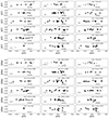 |
Fig. A.1. Δ(Y) (upper) and Δ(Ba) (lower) as a function of Δ(Na) for each cluster of the sample. Filled squares and empty triangles represent actual measurement and upper limits, respectively. |
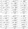 |
Fig. A.2. Δ(Y) (upper) and Δ(Ba) (lower) as a function of Δ(Na) for each cluster of the sample. Filled squares and empty triangles represent actual measurement and upper limits, respectively. |
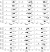 |
Fig. A.3. Δ(Y) (upper) and Δ(Ba) (lower) as a function of Δ(Na) for each cluster of the sample. Filled squares and empty triangles represent actual measurement and upper limits, respectively. |
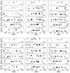 |
Fig. A.4. [La/Fe] (upper) and [Eu/Fe] (lower) as a function of Δ(Na) for each cluster of the sample. Filled squares and empty triangles represent actual measurement and upper limits, respectively. |
All Tables
Lines used for the abundance determination of heavier elements in the present extended survey.
Element sensitivity to the parameter variations (ΔTeff = +50 K, Δlog g = +0.2 dex, Δ[Fe/H] = +0.10, and Δvt = +0.10).
All Figures
|
Fig. 1. Example of the synthesised lines for one star of our sample (NGC 2808−49743). The red line represents the best fit. Blue and green fits correspond to the best fit of each element ±0.1 dex, respectively. |
| In the text | |
|
Fig. 2. Δ(Cu)MEAN along with vt for each GC of the sample. The respective Spearman corr. and p-values are indicated on each panel. Filled circles and empty triangles represent actual Cu measurements and upper limits, respectively. |
| In the text | |
|
Fig. 3. Pair of stars of the GC NGC 6171 with similar stellar parameters as reported by Carretta et al. (2009), a different Cu abundance. Black and red lines represent the spectra of ID = 19956 and ID = 7948, respectively. |
| In the text | |
|
Fig. 4. [Cu/Fe] distribution along with Δ(Na) for each GC analysed. The respective average and standard deviation Cu abundance are indicated in solid and dashed lines, respectively. Symbols follow the same description as in Fig. 2. |
| In the text | |
|
Fig. 5. [Cu/Fe] distribution along the [Fe/H] for the whole sample. The analysed GCs are shown with coloured squares. Grey crosses show the field star abundances from Ishigaki et al. (2013). Red-filled crosses display the reported abundance of Cu in different GCs in the literature. Black circles represent results reported by Simmerer et al. (2003) for our in-common GCs (linked with a black dashed line). |
| In the text | |
|
Fig. 6. Pair of stars of the GCs NGC 2808 (ID = 8739; red line) and NGC 6121 (ID = 27448; black line) with similar stellar parameters and different Cu abundance. |
| In the text | |
|
Fig. 7. [Y/Fe] ([Ba/Fe]) abundances and Δ(Y) (Δ(Ba)), respectively, as a function of vt for the GC NGC 1904, shown in the upper (lower) left and right panels. The blue dotted line shows the linear fit. |
| In the text | |
|
Fig. 8. Comparison of Ba abundances obtained in the present article with D’Orazi et al. (2010) for in-common GCs. The average difference between our and their results, |
| In the text | |
|
Fig. 9. ΔY (upper panels) and ΔBa (lower panels) as a function of ΔO for the whole survey sample (except for NGC 7078). The sample was divided into three metallicity bins: [Fe/H] < −1.80 dex (metal-poor; left panels), −1.80 dex < [Fe/H] < −1.10 dex (metal-mid; mid-panels), and [Fe/H] > −1.10 dex (metal-rich; right panels). The respective Spearman coefficient and p-value are reported on each panel. |
| In the text | |
|
Fig. 10. ΔY (upper panels) and ΔBa (lower panels) as a function of ΔNa. It follows the same description as Fig. 9. |
| In the text | |
|
Fig. 11. ΔY (upper panels) and ΔBa (lower panels) as a function of ΔMg. It follows the same description as Fig. 9. |
| In the text | |
|
Fig. 12. [Y/Fe], [Ba/Fe], [La/Fe], and [Eu/Fe] as a function of the [Fe/H] for the whole sample, shown from top to bottom. Coloured squares represent the GCs analysed in the present sample. Red-filled crosses represent GCs abundance from the literature as in Fig. 5. Grey dots show the field star abundances, and grey crosses represent bonafide Halo field stars ([Mg/Fe] > 0.2 dex) taken from the SAGA database (Suda et al. 2008). |
| In the text | |
|
Fig. 13. Abundance ratios of [Ba/Eu] and [Ba/Y]s as a function of [Fe/H], respectively, shown in the left and right panels. Dashed lines at [Ba/Eu] 0.70 dex and −0.70 dex indicate the ratio for a full s-process and full r-process enrichment. The dashed line at [Ba/Eu] 0.00 dex displays the solar ratio. Magenta diamonds in the right-hand panel show dwarf galaxies results taken from Suda et al. (2008). Other symbols and colours follow the description given in Fig. 12. |
| In the text | |
|
Fig. 14. Pair of stars with similar stellar parameters and Na abundances as was reported by Carretta et al. (2009), but different n-capture abundances. From left to right: Y line at 4883 Å, Ba line at 5853 Å, La line at 6391 Å, and Eu line at 6645 Å. |
| In the text | |
|
Fig. 15. Comparison between the n-capture element abundances measured in the present work and modelled abundances from Cescutti & Chiappini (2014) coloured-coded by the logarithmic number of stars in each bin. |
| In the text | |
|
Fig. 16. IQRs for Y, Ba, La, and Eu abundances as a function of the absolute visual magnitude for the whole sample. The MV values were taken from the Harris catalogue (Harris 2010). |
| In the text | |
|
Fig. A.1. Δ(Y) (upper) and Δ(Ba) (lower) as a function of Δ(Na) for each cluster of the sample. Filled squares and empty triangles represent actual measurement and upper limits, respectively. |
| In the text | |
|
Fig. A.2. Δ(Y) (upper) and Δ(Ba) (lower) as a function of Δ(Na) for each cluster of the sample. Filled squares and empty triangles represent actual measurement and upper limits, respectively. |
| In the text | |
|
Fig. A.3. Δ(Y) (upper) and Δ(Ba) (lower) as a function of Δ(Na) for each cluster of the sample. Filled squares and empty triangles represent actual measurement and upper limits, respectively. |
| In the text | |
|
Fig. A.4. [La/Fe] (upper) and [Eu/Fe] (lower) as a function of Δ(Na) for each cluster of the sample. Filled squares and empty triangles represent actual measurement and upper limits, respectively. |
| In the text | |
Current usage metrics show cumulative count of Article Views (full-text article views including HTML views, PDF and ePub downloads, according to the available data) and Abstracts Views on Vision4Press platform.
Data correspond to usage on the plateform after 2015. The current usage metrics is available 48-96 hours after online publication and is updated daily on week days.
Initial download of the metrics may take a while.