| Issue |
A&A
Volume 696, April 2025
|
|
|---|---|---|
| Article Number | A1 | |
| Number of page(s) | 14 | |
| Section | Interstellar and circumstellar matter | |
| DOI | https://doi.org/10.1051/0004-6361/202453273 | |
| Published online | 31 March 2025 | |
Resolved gas temperatures and 12C/13C ratios in SVS13A from ALMA Observations of CH3CN and CH313CN
1
Max-Planck-Institut für extraterrestrische Physik,
Giessenbachstrasse 1,
85748
Garching, Germany
2
Taiwan Astronomical Research Alliance (TARA),
Taiwan
3
Institute of Astronomy and Astrophysics, Academia Sinica,
PO Box 23-141,
Taipei
106, Taiwan
4
Department of Physics and Astronomy, University of Rochester,
Rochester,
NY
14627, USA
5
European Southern Observatory,
Karl-Schwarzschild-Strasse 2
85748
Garching bei Munchen, Munchen,
Germany
6
Univ. Grenoble Alpes, CNRS, IPAG,
38000
Grenoble,
France
7
Institut de Radioastronomie Millimétrique,
300 rue de la Piscine, Domaine Universitaire,
38406
Saint-Martin d’Hères, France
★ Corresponding author; This email address is being protected from spambots. You need JavaScript enabled to view it.
Received:
3
December
2024
Accepted:
4
February
2025
Abstract
Context. Multiple systems are common in field stars and the frequency is found to be higher in early evolutionary stages. Thus, the study of young multiple systems during the embedded stages is key to a comprehensive understanding of star formation. In particular, the way material accretes from the large-scale envelope into the inner region and how this flow interacts with the system physically and chemically has not been well characterized observationally to date.
Aims. We aim to provide a snapshot of the forming protobinary system SVS13A, consisting of VLA4A and VLA4B. This includes a clear picture of its kinematic structures, physical conditions, and chemical properties.
Methods. We conducted ALMA observations toward SVS13A targeting CH3CN and CH313CN J=12-11 K-ladder line emission with a high spatial resolution of ∼30 astronomical units (au) at a spectral resolution of ∼0.08 km s−1 .
Results. We used local thermal equilibrium (LTE) radiative transfer models to fit the spectral features of the line emission. We found the two-layer LTE radiative model that includes dust absorption is essential to interpreting the CH3CN and CH313CN line emission. We identified two major and four small kinematic components and derived their physical and chemical properties.
Conclusions. We identified a possible infalling signature toward the bursting secondary source VLA4A, which may be fed by an infalling streamer from the large-scale envelope. The mechanical heating in the binary system, as well as the infalling shocked gas, are likely to play a role in the thermal structure of the protobinary system. By accumulating mass from the streamer, it is plausible that the system experienced a gravitationally unstable phase before the accretion outburst. Finally, the derived CH3CN/CH313CN ratio is lower than the canonical ratio in the ISM and varies between VLA4A and VLA4B.
Key words: accretion, accretion disks / radiative transfer / binaries: close / stars: formation / ISM: kinematics and dynamics
© The Authors 2025
 Open Access article, published by EDP Sciences, under the terms of the Creative Commons Attribution License (https://creativecommons.org/licenses/by/4.0), which permits unrestricted use, distribution, and reproduction in any medium, provided the original work is properly cited.
This article is published in open access under the Subscribe to Open model.
Open Access funding provided by Max Planck Society.
1 Introduction
Observations have revealed that the frequency of multiple stellar systems increases during earlier evolutionary stages, with a multiplicity rate of 0.57 for Class 0 and 0.23 for Class I (Tobin et al. 2018; Offner et al. 2023). Multiple systems are also commonly observed among field stars (Tokovinin 2014). Thus, to understand the most common pathway of star formation, it is essential to study multiple systems at early stages (e.g., Murillo et al. 2024).
In contrast to the classical picture, suggesting that stars form through the isotropic collapse of dense cores (Shu 1977; Terebey et al. 1984), recent molecular line observations have revealed non-axisymmetric accretion in progress (Pineda et al. 2023). This infalling material is distributed in spatially elongated yet narrow structures, named “infalling streamers”, which have been seen at different evolutionary stages (Yen et al. 2019; Pineda et al. 2020; Alves et al. 2020; Ginski et al. 2021; Murillo et al. 2022a; Cabedo et al. 2021; Garufi et al. 2022; Thieme et al. 2022; Valdivia-Mena et al. 2022, 2024; Flores et al. 2023; Gupta et al. 2024). These infalling streamers can significantly contribute to the mass accretion rate from the core to disk, ~10−6 M⊙ yr−1 (Valdivia-Mena et al. 2022). Infalling streamers are also seen in numerical simulations, such as those of Kuffmeier et al. (2017). In addition, infalling streamers might play a crucial role in changing the physical structures and chemical compositions in the inner region (Garufi et al. 2022; Podio et al. 2024). The complex organic molecule (COM) CH3CN, with its K-ladder transitions, is widely used as a thermometer toward hot dense regions. It is more commonly seen in high-mass star-forming regions, but has also been found in low-mass star-forming regions (Bottinelli et al. 2007; Bisschop et al. 2008; Bergner et al. 2018; Loomis et al. 2018; Calcutt et al. 2018; Belloche et al. 2020; Yang et al. 2021).
SVS13A is a well studied protobinary system located in the NGC 1333 cluster in the Perseus Molecular Cloud (d =293 pc, Ortiz-León et al. 2018). It is a Class I close binary consisting of VLA4A and VLA4B (or Per-emb-44B and 44A) with a separation of 0′.′3 (~90 au) based on continuum emission (Anglada et al. 2004; Tobin et al. 2018; Segura-Cox et al. 2018). Diaz-Rodriguez et al. (2022) derive the total mass of the binary as l.0 ± 0.4 M⊙, given the proper motion of the binary orbit. The individual masses of the protostars are estimated as 0.27±0.10 M⊙ for VLA4A (secondary) and 0.60±0.20 M⊙ for VLA4B (primary). The SVS13A binary system has a high bolometric luminosity of Lbol = 45.3 L⊙ likely because the secondary VLA4A is in an outburst phase (Hsieh et al. 2019). In addition, Hsieh et al. (2023) found a large-scale (~700 au) candidate streamer connected with the dusty spiral linked to VLA4A. This streamer is possibly infalling, funneling material to the binary system with a mass infall rate >1.4 × 10⁻⁶M⊙ yr−1. We know that CH3CN and the isotopologs CH2DCN and CH313CN have been previously detected toward SVS13A (Bianchi et al. 2019; Hsieh et al. 2023; Bianchi et al. 2022a); however, the emission had not been spatially resolved. Observations of O-bearing COMs at a ~300 au resolution in Hsieh et al. (2024) indicated that multiple structures are expected to exist on scales of tens of astromonical units (au), based on multiple velocity components.
In this work, we present new Atacama Large Millimeter ter/submillimeter Array (ALMA) molecular line observations of CH3CN and CH313CN towards SVS13A. We resolve the emission from the COM species CH3CN and CH313CN down to 30 au (0.1 arcsecond). The high angular and spectral resolution data resolved the line emission, tracing the disks or rotating envelope around the protobinary VLA4A and VLA4B. In Sect. 2, we present the data and imaging process. The results are reported in Sect. 3. In Sect. 4, we discuss the LTE radiative transfer fitting and identify the kinematic components. The discussions and conclusions are in Sects. 5 and 6, respectively.
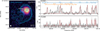 |
Fig. 1 Left: integrated intensity map of the CH3CN J=12-11 K=3 ladder with the contours from 1.3 mm continuum at levels of 3, 5, 7, 10, 20, 40, 100, and 200σ, with σ = 0.2 K. Right: sSpectra seen from the cross-marked positions of VLA4A (top) and VLA4B (bottom) from the CH3CN window. The red lines represent the best fits from our models (see Sects. 4.2.1 and 4.2.2). |
2 Observations
2.1 ALMA observation
We conducted ALMA observations in June 2023 with three executions, designated by the project ID 2022.1.00479. In these executions, 43–45 antennas were used. PWV among the observations were from 0.4 to 0.55 mm. With the ALMA C-7 configuration, the baselines were 91-8282 m (~65–6000 kλ) at 220 GHz, recovering scales from 0.1 to 1.2 arcsec (~30–360 au). The total on-source (SVS13A) time was 144 min toward the phase center at International Celestial Reference System (ICRS) α = 3h29m 03s.74, δ = 31d16m03s.8. The three executions shared the same bandpass and flux calibrator as J0423-0120, while the phase calibrator was either J0328+3139 or J0336-3218, depending on the execution.
The observations were designed to observe multiple chemical and kinematic tracers toward SVS13A, so that multiple high-resolution spectral windows were placed accompanied with one continuum window at 234.5 GHz with 1.875 GHz bandwidth and 488 kHz (0.6 km s−1) channel width (band 6, Ediss et al. 2004). In this paper, we present the CH3CN J=12-11 window, which covers a wavelength ranging from 220.52 to 220.75 GHz with a channel width of 61 kHz (0.08 km s−1). We use the pipeline calibrated data restored using CASA 6.4.12 (CASA Team et al. 2022). The imaging was done using the tclean package with a robust weighting of 0.5, resulting in a beam size of 0′.′ × 0′.′08 (~30 au) for the CH3CN cube. This image cube has an rms noise level of 1.7 mJy beam−1 (4.7 K) at the spectral resolution of 0.08 km s−1.
2.2 STATCONT for continuum subtraction
Many spectral lines adding up to ‘forest’ features have been seen in high-mass star forming regions (Sánchez-Monge et al. 2018), making the determination of the continuum level difficult. This may also happen in low-mass star forming regions for the chemically-rich sources, for instance, hot corinos (Ceccarelli 2004), especially with high-sensitivity data.
SVS13A, with its high luminosity (45.3 L⊙), has plenty of line features already known in the literature (Bianchi et al. 2019, Bianchi et al. 2022b; Diaz-Rodriguez et al. 2022; Hsieh et al. 2023); as shown in Fig. 1. We used STATCONT (Sánchez-Monge et al. 2018) to determine the continuum level and find the line-free channels. STATCONT performs a continuum subtraction in the image domain pixel by pixel, providing a continuum-subtracted cube and continuum image as outputs. We used the default sigmaclipping algorithm, which removes the line-emitting channels by iteratively measuring the median and standard deviation in a histogram of spectral points. Thus, we obtained the continuum image from the continuum window and the line image cube from the CH3CN window.
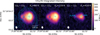 |
Fig. 2 Integrated intensity map of the CH3CN J=12-11 with K=0, 3, and 7. The integration range is 4–12 km s−1. The contours represent the 1.3 mm continuum emission at levels of 3, 5, 10, 20, 50, 150, and 300σ with σ =0.2 K. The blue cross markers indicate the locations of VLA4A and VLA4B from the continuum emission. |
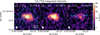 |
Fig. 3 Same as Fig. 2, but for the integrated intensity map of the CH313CN J=12-11 with k=1, 2, and 5. The integration range is 5.5–11 km s−1 . |
3 Results
3.1 Continuum emission
Figure 1 shows the continuum image as contours. The binary components feature VLA4A as the secondary and VLA4B as the primary, which are well resolved, and two spirals are seen, in line with previous observations (Tobin et al. 2018; Diaz-Rodriguez et al. 2022). The continuum emission from the secondary (VLA4A) is more extended than that of the primary. However, VLA4A peak brightness is lower (70 K) than the primary VLA4B (90K). The relative brightness is consistent with that at 0.9 mm, 260 K for VLA4A and 430 K for VLA4B (Diaz-Rodriguez et al. 2022). It is likely that the inner 30 au region is optically thick for both VLA4A and VLA4B at 0.9 mm, as previously seen for other compact binary system (e.g., Maureira et al. 2022). In this case, the difference could indicate either a lower dust temperature for the secondary or higher amounts of material therein, leading to higher levels of selfobscuration (e.g., Galván-Madrid et al. 2018). It is likely that VLA4A is the more active source during an accretion outburst (Hsieh et al. 2019), also given its connection to the potential infalling streamer (the spiral) and the spectral features discussed below.
3.2 CH3CN and CH313CN
Both the CH3CN and CH313CN J = 12–11 emission is spatially resolved toward SVS13A. The K-ladder is detected in the observing windows with K = 0–7 for CH3CN and K = 0–5 for CH313CN (Fig. 1). Given the forest of lines, one particular line can be severely contaminated by other molecules, especially for CH313CN. Furthermore, CH3CN emission is relatively strong but is still partially affected by a few bright lines such as CH3OCHO and C2H5OH (see Fig. 2 in Hsieh et al. 2023). Using the broad wavelength coverage provided by the large program PROtostars & DIsks: Global Evolution (PRODIGE) using NOEMA, Hsieh et al. (2023, 2024) thoroughly identify the molecular lines by performing LTE modeling for each molecule with multiple transitions. However, there are still unidentified lines in the spectral window considered here (Fig. 1).
In Figs. 2 and 3, we show the integrated intensity maps from three transitions of CH3CN and CH313CN, cover different energy levels and suffer less from contamination. For CH3CN, it is clear that the emission peaks towards VLA 4A, while for CH313CN, the emission peaks in the region between the protostars. In addition, a ring-like emission surrounding VLA4B from CH3CN and CH313CN is revealed, especially for the lines with lower upper energy levels, for which the emission is also the brightest. Such a ring structure has been found in other sources such as V883 Ori (Lee et al. 2019; Yamato et al. 2024). This can be interpreted either being due to the high optical depths of the dust or to the destruction of COMs in the inner disk via strong UV or X-ray radiation (Garrod & Herbst 2006; Öberg et al. 2009). An extreme case for this absorption is found in NGC 1333 IRAS 4A1, with absorption line features (Sahu et al. 2019). For SVS13A VLA4B, we favor the high dust optical depth scenario because: (1) VLA4B does indeed exhibit stronger continuum emission than VLA4A; and (2) the UV radiation is likely to be more powerful in VLA4A, as the source is undergoing an accretion burst (Hsieh et al. 2019).
Although the CH3CN line emission is dominated by VLA4A, the CH313CN emission peak is located between VLA4A and VLA4B. It is unclear at the current stage if this is the material interacting between the binary system (Jørgensen et al. 2022). This is consistent with the result from Hsieh et al. (2023), who speculated that the CH3CN and CH313CN emission comes from different regions or layers, due to the different optical depths. With the resolved map, we can clearly see the spatial difference, even in the optically thin emission, namely, K=7 from CH3CN. In other words, these results suggest a spatially inhomogeneous isotopolog ratio of CH3CN/CH313CN toward the protobinary SVS13A.
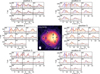 |
Fig. 4 Spectra of CH3CN toward SVS13A at selected positions marked in the central image of the K=3 integrated intensity map. In the central image, the white contours represent the S/N of 3 and 12, as the latter represents the region where LTE fitting is made. The blue stars indicate the positions of VLA4A and VLA4B. The kinematic components II-VI (II: red, III: green, IV: orange, V:purple, VI: yellow; see Fig. 6) are shown as contours in different colors and for the positions within a contour, the two-layer LTE model is used for fitting (see Sect. 4.3). Each spectrum has been divided to eight individual panels centering at the Vlsr, i.e., 7.36 km s−1 for VLA4A and 9.33 km s−1 for VLA4B (Diaz-Rodriguez et al. 2022 blue and red dashed vertical lines in the K=0 panel), of the K-ladder. The red spectra show the best-fit from the LTE model while the color areas show the two-layer model with front (1, orange) and rear (2, purple) layers. We note that Eq. (2) is more complicated, so this colored area is only meant to offer an general view of Vlsr and ∆V. |
4 Analysis
4.1 LTE model setup
We applied local thermal equilibrium (LTE) modeling to the CH3CN and CH313CN lines for the whole map (pixel by pixel). A spatial mask was taken, using a signal-to-noise ratio threshold of S/N>12 from the CH3CN K=3 integrated intensity map (Fig. 4). To avoid the contamination from other lines, a selected mask at specific velocities was provided manually (e.g., the blue-shifted side in CH3CN K=6 or CH313CN K=3 components). The LTE model is constructed based on CASSIS and XCLASS manuals (Vastel et al. 2015; Möller et al. 2017). The line data were taken from CDMS (Müller et al. 2005; Endres et al. 2016) and JPL (Pickett et al. 1998), whereas the original catalogs are from (Müller et al. 2009, 2015). The details are in Appendix A.1.
 |
Fig. 5 Fitting results of the one-layer LTE model. Each panel shows a map of the free parameter with the label of the colorbar on the top. The contours on the first panel represents the 1.3 mm continuum emission (Fig. 2). The contours of the second column represents τ at 1 and 2, while those in the sixth column show the isotopolog ratios of 15 and 68. The fourth column gives the Vlsr map, where the systemic velocities of VLA4A and VLA4B are 7.36 and 9.33 km s−1, respectively (Diaz-Rodriguez et al. 2022). |
4.2 Radiative transfer model
We performed LTE modeling throughout the emitting regions pixel by pixel, adopting a one- or two-layer model. Here, we introduce the two models and present the model selection in Sect. 4.3.
4.2.1 One-layer model
We first conducted single velocity component LTE modeling, which takes into account dust absorption. This approach assumes that the dust and gas are co-located, instead of assuming the dust as a background to the gas (see Sahu et al. 2019; Rosotti et al. 2021; Bosman et al. 2021; Yamato et al. 2024), and that the dust and gas temperature are the same, Tex . The continuum subtracted spectrum is thus
![Mathematical equation: ${I_v}(\v ) = \left[ {{J_v}\left( {{T_{{\rm{ex}}}}} \right) - {J_v}\left( {{T_{{\rm{bg}}}}} \right)} \right]\left( {1 - {e^{ - \tau (v)}}} \right){e^{ - {\tau _{{\rm{dust}}}}}},$](/articles/aa/full_html/2025/04/aa53273-24/aa53273-24-eq1.png) (1)
(1)
where Tbg = 2.7 K, τ(υ) is the line optical depth, and τdust is the dust optical depth. The detailed derivation can be found in Appendix A.2. As a result, we obtained a scale factor of exp (−τdust), which fills the same role as it does in Hsieh et al. (2023, 2024), where a beam-filling factor was used to scale the emission. At the edge of the emitting area, a beam might cover a partially line-free region where a beam-filling factor would be needed, so the τ value might be overestimated. We chose a high S/N of 12 as a mask in the integrated intensity map of K=3 to avoid this. We note that an LTE model without considering dust absorption was also tested, but it failed to interpret the line spectrum; without the scaling factor,  , the model naturally would underestimate the column density with a small τ to fit the absolute brightness of the observed spectrum, resulting an inconsistent line ratio.
The spectra in Figs. 1 (position VLA4B) and 4 (positions 2 and 5) show the one-layer model fit toward these positions. Figure 5 shows the maps of the six free parameters from the fit. The temperature peaks toward VLA4A. We note that the partition function Q(T) is provided by CDMS up to 900 K, so the boundary of the fitting was set to 800 K. The derived τdust from the line fit is quite similar to the continuum emission, supporting the notion that the dust optical depths are reasonably estimated. The peak τ ~ 2.5 suggests that only ~10% of line emission might escape from these regions. There are also regions with τ < 1, suggesting the continuum emission is not optically thick through the entire line-emitting region. Thus, it is reasonable to assume a coupling of gas and dust, rather than an optically thick continuum emission as background. CH3CN column density is higher toward VLA4A, as expected. The Vlsr and FWHM maps are generally similar to the average-velocity maps and moment 2 maps from previous high-resolution COM maps (Diaz-Rodriguez et al. 2022; Bianchi et al. 2022b). The isotopolog ratio CH3CN/CH313CN is taken as (see Eqs. (A.1) and (A.2)). As a result, the spatially inhomogeneous distribution is presented.
4.2.2 Two-layer model
Although the LTE model with dust absorption is able to interpret the relative intensities of the K-ladder transitions, the high spectral resolution data reveal double-peak features in some areas (Fig. 4). Hsieh et al. (2024) conducted multi-component LTE fitting of O-bearing COMs toward SVS13A, decomposing different kinematic components. In that work, the kinematic components are assumed to be spatially separated within the NOEMA beam. However, with the spatially-resolved ALMA map, the double peak spectral profiles are still present in particular regions, indicating two components along the line of sight. Thus, we conduct the two-layer LTE model to interpret these spectra. Each layer has its own excitation temperature (Tex), dust optical depth (τdust), CH3CN column density (Ntot), central velocity (VLSR), linewidth (ΔV), and isotopolog ratio (CH3CN/CH313CN); twelve free parameters are included. The continuum subtracted spectrum is
![Mathematical equation: $\eqalign{ & {I_v}(\v ) = \left[ {{J_v}\left( {{T_{{\rm{ex}},1}}} \right) - {J_v}\left( {{T_{{\rm{ex}},2}}} \right)} \right]\left( {1 - {e^{ - {\tau _1}(\v )}}} \right){e^{ - {\tau _{{\rm{duss }},1}}}} \cr & \,\,\,\,\,\,\,\,\,\,\,\, + \left[ {{J_v}\left( {{T_{{\rm{ex}},2}}} \right) - {J_v}\left( {{T_{{\rm{bg}}}}} \right)} \right]\left( {1 - {e^{ - \left[ {{\tau _1}(\v ) + {\tau _2}(\v )} \right]}}} \right){e^{ - \left( {{\tau _{{\rm{dass }},1}} + {\tau _{{\rm{dust }},2}}} \right)}}, \cr} $](/articles/aa/full_html/2025/04/aa53273-24/aa53273-24-eq4.png) (2)
(2)
and the detailed derivation is in Appendix A.3. This equation can be considered as a variation from the two-layer model in Myers et al. (1996) and its family (Lee et al. 2001; Di Francesco et al. 2001; De Vries & Myers 2005; Kang & Kerton 2012). The original two-layer model is applied to infall motion at molecular core where the dust absorption might be negligible. Equation (2) will converge to the original two-layer model when τdust,1 = 0 and τdust,2 = 0. In addition, the original two-layer model assumes two uniform layers with the same optical depth τ(υ) (see Eq. (A.1)) as symmetrically infalling. Here, the LTE model requires number densities of population for energy levels (defining τ) to follow the Boltzmann distribution with the given Tex (Eqs. (A.2) and (A.3)). We find that a symmetric model, namely, with the same velocity dispersion, σ, and Ntot for the two layers, is insufficient for some regions (e.g., position 4 in Fig. 4 with linewidths of 0.9 and 1.5 km s−1 for the first and the second layer, respectively). It is noteworthy that this two-layer model will also converge to the gas-dust decoupling model when τdust,1 = 0 (gas front layer) and τ2(υ) = 0 (dust rear layer) as Rosotti et al. (2021). Clearly, if we have an optically thick dust continuum as the rear layer (τdust,2 ≫ 1), only the first term in Eq. (2) is left, with Tex,2 representing the background temperature of the dust layer.
We performed the fit throughout the line-emitting region (Fig. 4). Carrying out such a fit with so many free parameters is difficult to converge and, thus, it suffers from degeneracy (see Appendix B). To address these issues, good initial guesses are required. We first perform Markov chain Monte Carlo (MCMC) sampling of a grid of positions in the emitting regions (in total 41 positions with gaps around emission of roughly beam size). We tuned the sampling boundary (prior range) of the MCMC fitting and found the most reasonable solution. For example, the fitting results should not show any dramatic difference in between two neighboring positions. These solutions at each points in the grid are then interpolated to a map of initial guesses for the fitting. Figure 4 shows the spectra of a few selected positions for which the best fits from MCMC sampling are plotted (with a one- or two-layer model; see Sect. 4.3).
4.3 Clustering into kinematic components
Here, we discuss how we selected a one- or two-layer model in each pixel and clustered them into kinematic components. We used the following criterion for the two layer-model: the difference among the centroid velocities (Vin = VLSR,1 − VLSR,2) is larger than the velocity dispersions of both layers, σ1 and σ2 . This threshold set a strict situation for using two-layer model only when the double-peak is clearly seen in the position. For example, in Fig. 4, for positions 4 and 5, when using one-layer model, the spectral profiles in fact shows blue or red asymmetry, which is considered as an indicator of infall or expansion motions in cloud cores (Mardones et al. 1997; Tafalla et al. 1998; Lee et al. 2001; Emprechtinger et al. 2009; Pineda et al. 2012; Hsieh et al. 2015; Redaelli et al. 2022). Although the two-layer model better reproduces the spectra profile with lower reduced χ2 and Akaike information criterion (AIC; see Appendix B), the one-layer model is chosen in cases where no clear double peak is presented. It is possible that the two layers are blended with similar centroid velocities or broad linewidths. For example, in Fig. 7 in Bianchi et al. (2017), with respect to CH3OH isotopologs toward SVS13A, a broken power law is seen in the rotation diagram, decomposing components without spatially or spectrally resolved data. However, in our case, with only eight energy levels from CH3CN J=12–11 K=0–7 (in the rotational diagram), we decided to be more conservative, using a one-layer model for positions without a clear double peak. More importantly, to study the kinematic structure, these regions with small relative velocity between two layers (see also Fig. B.2, right panel) will not be decomposed or extracted as a new kinematic component by the clustering algorithms in the position-position diagram.
After the model selection, we obtained a final map at each position containing one or two velocity components (from the one- or two-layer model respectively). Figure 6 shows the position-position-velocity diagram (PPV), as it is better at decomposing the CH3CN distribution than P-V diagrams. We use the clustering algorithm DBSCAN (Ester et al. 1996; Valdivia-Mena et al. 2023; Gieser et al. 2024), with eps=0.3 and min_samples=10, clustering these points into six groups. For discarded points, we simply use the one-layer model at such positions, so they go back to the major kinematic component I (Fig. 6). As a result, two major kinematic components, I and II, and four small components III-VI have been identified (Fig. 6). Table 1 lists their physical parameters. Because the two-layer model does, in fact, determine the front layer and the rear layer (i.e., as shown by Eq. (2)), then the infall or expansion of the two layers can be obtained. A positive value of Vin in Table 1 indicates expanding motion, while a negative one indicates an infalling motion (Myers et al. 1996; Mardones et al. 1997). However, there is a caveat to determine this given the degeneracy of the model. For example, although the double peak profiles with a blue excess are clearly seen toward the region with component II as infalling signatures, we can find another fit for expanding motion due to the asymmetric layers (see Appendix B for the degeneracy). To completely break the degeneracy, multi-band observations would help with measuring dust opacity at different wavelengths (e.g., optically thick dust emission as Pineda et al. 2012). Finally, the absolute value of the relative velocity of each component with respect to component I is presented in Fig. 7. Figure 8 shows the best-fit parameters of all six components and Table 1 lists them.
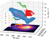 |
Fig. 6 PPV diagram from the combination of one- and two-layer model fitting. The bottom x-y image is the CH3CN J=12-11 K=3 integrated intensity map. Above it, each position can have one or two velocities. The color of data points indicates the kinematic component from clustering. The two cyan vertical lines indicates the positions and the systemic velocities of VLA4A (7.36 km s−1) and VLA4B (9.33 km s−1). |
5 Discussion
5.1 Kinematic structures
The velocity map shown in panel d of Fig. 5 generally reveals similar structures to average-velocity maps from the literature (Diaz-Rodriguez et al. 2022; Bianchi et al. 2022b). However, our two-layer model is aimed at an ambitious study of the motion along the line of sight of the system (Fig. 8). The velocity gradient along west-east of the major component I is greater than that in the one-layer model, because at the west side, the red- shifted emission is decomposed to the component II. Figure 7 shows the absolute value of the relative velocity, |δVrelative|, of these components with respect to the main component I. A major portion of Component II is around VLA4A, which is perhaps also affected or induced by the dusty spiral, considered here as a possible infalling streamer (Hsieh et al. 2023).
Figure 7 reveals a velocity pattern (|δVrelative|) of component II relative to I with a radial symmetric structure centered to the west of VLA4A. We note again that although the two-layer model has defined front and rear layers with different velocities, these two layers can frequently be difficult to disentangle (see Appendix B). Thus, we were not able to determine if it is an infall or outward motion only from the spectra. However, the majority of component II indicates that the blue excess favors the infall motion. In addition, the radial symmetric structure in Fig. 7, namely, the relative velocity between component I and II, implies that this traces an infall motion centering around VLA4A. If this is the case, it might help us better understand the nature of the possible infalling streamer (Hsieh et al. 2023). In this case, the secondary source, VLA4A, is fed by the infalling streamer during an accretion outburst. One caveat is that the possible infalling streamer found by Hsieh et al. (2023) via DCN has a landing velocity at the blue-shifted emission 7–8 km s−1 , similar to that of C18O from the spiral (Tobin et al. 2018). This is different from the component II with velocity around 9 km s−1 (Table 1 and Fig. 8). This implies that the component II from the CH3CN emission is not directly associated with the dusty spiral.
Regarding the rotation, Diaz-Rodriguez et al. (2022) found a disk surrounding VLA4A and a circumbinary disk via ethylene glycol and CS observations, respectively. The Vlsr maps from our LTE fitting, namely, panel d in Fig. 5, are broadly similar to the mean-velocity map in Diaz-Rodriguez et al. (2022). The S- shape pattern in between the blue- and red-shifted emission can be explained by the simultaneous presence of infall and rotation (Flores et al. 2023). We looked at position-velocity (PV) diagrams (Figs. C.1 and C.2), where the position axis goes from west to east and passes through A and B. In the PV-diagrams, likely only the blue-shifted emission in the west of the Keplerian rotation is seen via CH3CN and CH313CN, as in component I (Fig. 8). Figure 9 compares the velocity pattern of component I with thin disk models given the parameters from Diaz-Rodriguez et al. (2022). These results are consistent with the literature and the model is able broadly describe the VLA4A disk; however, in VLA4B, there is no detection of a gas disk (see Figs. C.1 and C.2) for which the inclination angle is obtained from a dust continuum. This makes component II interesting in that it is likely to be associated with infalling materials, but not directly with the infalling streamer or the continuum spiral.
Kinematic components.
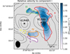 |
Fig. 7 Absolute relative velocity of the component II-VI with respect to the main component I. The contours represent the continuum emission with the same levels as Fig. 1. The color contours show the area of component II-VI. |
5.2 Physical conditions
Figures 5 and 8 show the gas temperature structures from the CH3CN K-ladder. The temperature map of the major component I is similar to that of the one-layer model. Both components I and II have a peak temperature toward VLA4A. This could also explain the high column density of CH3CN at VLA4A, where molecules are sublimated from the dust mantles.Component II is relatively cooler than component I (Table 1). As the component I is likely associated with the rotating disk or envelope around VLA4A (Figs. 6 and C.1), the component II might trace materials induced by the possible infalling streamer.
Radiation from central protostars is usually considered as the main heating source, used to determine the temperature from previous modeling works (Rab et al. 2017; Hsieh et al. 2018, 2019; Murillo et al. 2022b). Toward SVS13A, although the temperature is mostly determined by the protostellar radiation, it is unlikely to be the only factor involved in reproducing the asymmetric structure. First, toward VLA4B, the gas temperature in its west side is clearly higher than that in the east. It is likely that the circumbinary material in between VLA4A and VLA4B is relatively warmer. More interestingly, the temperature is relatively high along the spiral, represented by the possible infalling streamer (Figs. 5 and 8). Mechanical heating has been suggested as an explanation of the asymmetric temperature structures seen in IRAS 16293-2422 (Maureira et al. 2022). If the dusty spiral traces a streamer accreting onto the protostellar or circumbinary disk, it can induce shocked gas and heat up the material. For example, shocked gas traced via SO has been detected toward the landing position of an infalling streamer in HL Tau Garufi et al. (2022) and in Per-emb-50 Valdivia-Mena et al. (2022). High spatial and spectral resolution observations of SO might help disentangle the shocked gas induced in SVS13A.
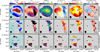 |
Fig. 8 Same as Fig. 5, but for the clustering components. Note: the discarded points are attributed to one-layer fitting in component I. The top, middle, and bottom panels show the parameters for component I, II, and III-VI, respectively. The fourth column shows the Vlsr map, with the systemic velocities of VLA4A and VLA4B calculated as 7.36 and 9.33 km s−1, respectively (Diaz-Rodriguez et al. 2022). |
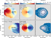 |
Fig. 9 Left column: velocity map of component I (Fig. 8) relative to VLA4A (top, VVLA4A = 7.36 km s−1) and VLA4B (bottom, VVLA4B = 9.33 km s−1). Middle: Keplerian disk model using the Mstar and θinc from Diaz-Rodriguez et al. (2022). We note that the inclination angle of VLA4B is from the dust continuum as the gas disk is not seen here. Right: Toomre Q map derived using the physical parameters from CH3CN plus models of rotation from the middle panel. |
5.3 Toomre Q analysis
Disk fragmentation is considered to part of the formation process of close binary systems (Offner et al. 2023). The Toomre Q parameter is widely used to test whether a disk is gravitationally unstable, as per
 (3)
(3)
where cS is the sound speed, Ω is the angular velocity, G is the gravitational constant, and Σ is the disk surface density (Toomre 1964). Here we use the Tex from the one-layer model to derive the sound speed (Fig. 5; see also Ahmadi et al. 2023). We use the τ map (Fig. 5) to estimate Σ, assuming the dust opacity κ = 0.899 cm2 g−1 at 1.3 mm (Ossenkopf & Henning 1994; Tobin et al. 2018), a gas to dust mass ratio of 100, with an inclination correction from Diaz-Rodriguez et al. (2022). It is noteworthy that the dust opacity can bring on an uncertainty in a factor of a few (Birnstiel et al. 2018). To estimate the angular velocity, we compared the velocity map from Fig. 8 and thin-disk models for VLA4A and VLA4B, given the star masses and inclination angle from Diaz-Rodriguez et al. (2022, as well as in our Fig. 9). We note here that component I in Fig. 8 was used because the one-layer velocity map (Fig. 5) includes the contribution from component II, with the red-shifted emission in the east (Figs. 8 and C.1). By assuming Keplerian rotation, we obtained Q maps for VLA4A and VLA4B (Fig. 9).
The Q parameter maps show that the disks are in general stable near the protostars (Q > 1). However, VLA4A is likely undergoing an accretion outburst, suggesting that the high temperature is temporary. If we assume T ∝ L0.2 (Goldreich & Kwan 1974), and the luminosity were to be 100 times lower during the quiescent phase, the cs value as well as the Q parameter would then be a factor of ~0.6 of the current values. This makes more of the area in the disk gravitationally unstable, so that the disk fragmentation might occur during the quiescent phase, causing the binary formation or triggering the accretion burst (Boley & Durisen 2008; Vorobyov & Basu 2005, 2010; Offner et al. 2009; Machida et al. 2011). In addition, VLA4A is surrounded by the potential infalling pattern (Fig. 7) and the possible infalling streamer Hsieh et al. (2023) which could be partly responsible for the accretion burst via gravitational instability (Pineda et al. 2023).
5.4 CH3CN/CH313CN spatial distribution
The 12C/13C ratio has been measured toward different protostellar systems Busch, L. (in prep.), and is usually found to be lower relative to the canonical ratio in the local ISM l2C/l3C≃68 (Milam et al. 2005). It is also found to vary at different distances from the central source (Yoshida et al. 2022, 2024; Bergin et al. 2024) Toward SVS13A, Hsieh et al. (2023) found a low value (16) and they suggested that the CH3CN and CH313CN might trace different regions or layers toward SVS13A. This is supported by the integrated intensity maps of Figs. 2 and 3. In other words, the isotopolog ratios can vary across SVS13A. With the LTE model (Figs. 5 and 8), we find low values in comparison with the canonical one throughout the maps except for component III and IV, but with large errors (Table 1). Other than these two components, the CH3CN/CH313CN ratios ~20–40 are generally lower than the canonical value of 68. Interestingly, it is even lower around the primary source VLA4B from both the one- and two-layer model (Figs. 5 and 8). This suggests a chemical segregation between VLA4A and VLA4B, as reported by Bianchi et al. (2022b) with other COMs. Furthermore, as the secondary VLA4A is likely connected to the dusty spiral, possibly tracing an infalling streamer (Hsieh et al. 2023), this hints that the infalling streamer might affect the chemistry in the inner region. For example, via H3CN, it has been suggested that an infalling streamer can deliver fresh chemical material from the cores into the disks in Per-emb-2 (Pineda et al. 2020).
6 Summary
We present CH3CN and CH313CN observations toward SVS13A using ALMA, with a spatial resolution of ~23 × 32 au and spectral resolution of ~0.08 km s−1. We conducted an LTE radiative transfer fitting of the line emission. Our main findings are summarized below:
The CH3CN and CH313CN integrated intensity is tracing material near both protostars, as well as material along the direction connecting both protostars. However, the CH3CN is brightest towards the secondary protostar VLA4A, while its 13C isotopolog is brightest in between the two protostars. In addition, toward the primary VLA4B, the emission from both CH3CN and CH313CN shows a dip at the location of the continuum peak, resulting in a ring-like morphology. This can be interpreted as dust absorption.
We modeled the lines from CH3CN/CH313CN considering the optical depth of the dust (i.e., dust absorption), assuming that the dust and gas are co-spatial and share the same temperature. We inferred temperatures ≳100 K in the line-emitting region, with the highest temperatures towards VLA4A (the secondary, >500 K), the region between the protostars (~300 K), and that along the possible infalling streamer (~250 K). The inhomogenous distribution of the temperature suggests that in addition to irradiation from the outbursting protostar VLA4A, there is also heating from shocks that has possibly been induced by an infalling streamer.
Toward some regions with resolved double-peak line profiles, we conducted two-layer LTE radiative transfer modeling to reproduce the features. This enabled us to identify two major kinematic components I and II. While component I is likely to be associated with rotating disk or envelope around VLA4A and VLA4B, component II might be associated with the dusty spiral structure, namely, a possible infalling streamer, around VLA4A. The velocities of this material differs from the main component by 1 to 3 km s−1 and could be connected to the infalling material towards the secondary VLA4A, which is undergoing an accretion burst.
Using the individual protostellar masses, the measured gas temperature for CH3CN and dust optical depth at 1.3 mm, we derived maps of the Toomre Q parameter around the protostars. We found broadly gravitationally stable disks (or rotating materials) with the current conditions. However, in the past, prior to the accretion outburst conditions experienced by VLA4A, the disk was cooled down and massive enough in some parts to become gravitationally unstable. It could have fragmented to trigger the binary formation or accretion bursts.
The CH3CN/CH313CN ratio is lower than the canonical 12C/13C ratio in the ISM over the whole region, but with variations across the map. The ratio towards the primary VLA4B, as well as for the material between the protostars, is around 10. On the other hand, the western part of the emission, which includes VLA4A, shows values between 15 and 50. Streaming material towards VLA4A could explain this difference.
Acknowledgements
We thank Dr. Naomi Hirano for the insight discussion. T.-H.H., J.E.P., P.C., M.T.V, and M.J.M. acknowledge the support by the Max Planck Society. T.-H.H. is supported by Taiwan Astronomical Research Alliance (TARA) with National Science and Technology Council (NSTC 113-2740-M- 008-005). TARA is committed to advancing astronomy in Taiwan and paving the way for the establishment of a national observatory. This paper makes use of the following ALMA data: ADS/JAO.ALMA#2022.1.00479.S. ALMA is a partnership of ESO (representing its member states), NSF (USA) and NINS (Japan), together with NRC (Canada), NSTC and ASIAA (Taiwan), and KASI (Republic of Korea), in cooperation with the Republic of Chile. The Joint ALMA Observatory is operated by ESO, AUI/NRAO and NAOJ. Software: Numpy (van der Walt et al. 2011), Scipy (Virtanen et al. 2020), APLpy (Astropy Collaboration 2013), Matplotlib (Hunter 2007), Astropy (Astropy Collaboration 2022) CASA (CASA Team et al. 2022).
Appendix A LTE Radiative transfer models
A.1 Boltzmann distribution and optical depth
LTE-radiative transfer model are constructed to fit the line profiles of the CH3CN J=12-11, K=0-7 and CH313CN J=12-11, K=0-5 transitions given the observed wavelength coverage. This is done following the XCLASS and CASSIS manuals1 (Möller et al. 2017) and (Vastel et al. 2015). The LTE τ(υ) as a Gaussian function of velocity (υ) was first constructed:
 (A.1)
(A.1)
where i is the transition including CH3CN and CH313CN, σ is the velocity dispersion  , VLSR is the centroid velocity,
 (A.2)
(A.2)
for which Aul is the Einstein coefficient, c is light speed, and ν is the rest frequency of the transition from the Cologne Database for Molecular Spectroscopy (CDMS2; Müller et al. 2005; Endres et al. 2016). Nu is the column density at the upper energy state as
 (A.3)
(A.3)
where gu is the degeneracy, Q(Tex) is the partition function, and Eu is the upper energy level. We note here the partition function Q(T) of CH313CN is taken from CH3CN due to the lack of the vibrational correction. This causes at most 0.06% error at T < 500 K (Hsieh et al. 2023).
A.2 Radiative transfer model with dust optical depth
Here we discuss the contribution of dust absorption in the LTE radiative transfer model. Under the LTE assumption with the same gas temperature and dust temperature (Tex = Tdust), the gas and dust are assumed to share the same space. The continuum-subtracted line emission with dust absorption can be expressed as:
![Mathematical equation: $\eqalign{ & \Delta {I_v}(\v ) = {I_{{\rm{line }}}}(\v ) - {I_{{\rm{dust }}}} \cr & \,\,\,\,\,\,\,\,\,\,\,\,\,\, = \left[ {{J_v}\left( {{T_{{\rm{bg}}}}} \right){e^{ - \left[ {\tau (\v ) + {\tau _{{\rm{dust }}}}} \right]}} + {J_v}\left( {{T_{{\rm{ex}}}}} \right)\left( {1 - {e^{ - \left[ {\tau (\v ) + {\tau _{{\rm{dust }}}}} \right]}}} \right)} \right] \cr & \,\,\,\,\,\,\,\,\,\,\,\,\, - \left[ {{J_v}\left( {{T_{{\rm{bg}}}}} \right){e^{ - {\tau _{{\rm{dust }}}}}} + {J_v}\left( {{T_{{\rm{ex}}}}} \right)\left( {1 - {e^{ - {\tau _{{\rm{dust }}}}}}} \right)} \right] \cr & \,\,\,\,\,\,\,\,\,\,\,\, = \left[ {{J_v}\left( {{T_{{\rm{ex}}}}} \right) - {J_v}\left( {{T_{{\rm{bg}}}}} \right)} \right]\left( {1 - {e^{ - \tau (v)}}} \right){e^{ - {\tau _{{\rm{dust }}}}}}. \cr} $](/articles/aa/full_html/2025/04/aa53273-24/aa53273-24-eq56.png) (A.4)
(A.4)
Here, in an optically thin case, τdust is 0, i.e.,  is ~1, so that the equation reverts to the commonly used equation. Here τ(υ) contains the following parameters: linewidth σ and central velocity VLSR as Gaussian profiles while the peak is determined by the column density Ntot and Tex (Eqs. A.1, A.2, and A.3). Together with the isotopolog ratio
  , six free parameters are included: excitation temperature (Tex), column density
  , dust optical depth (τdust), central velocity (VLSR), linewidth (ΔV), and isotopolog ratio
  .
.
A.3 Two layer LTE radiative transfer model
The two layer model simply adds one more layer with independent Tex , τ(υ), and τdust , so that:
![Mathematical equation: $\eqalign{ & \Delta {I_v}(\v ) = {I_{{\rm{line }}}}(\v ) - {I_{{\rm{dust }}}} \cr & \,\,\,\,\,\,\,\,\,\,\,\,\,\, = {J_v}\left( {{T_{{\rm{bg}}}}} \right){e^{ - \left[ {{\tau _1}(v) + {\tau _{{\rm{duss }},1}} + {\tau _2}(\v ) + {\tau _{{\rm{dust }},2}}} \right]}} \cr & \,\,\,\,\,\,\,\,\,\,\,\,\, + {J_v}\left( {{T_{{\rm{ex}},1}}} \right)\left( {1 - {e^{ - \left[ {{\tau _1}(\v ) + {\tau _{{\rm{dust }},1}}} \right]}}} \right) \cr & \,\,\,\,\,\,\,\,\,\,\,\, + {J_v}\left( {{T_{{\rm{ex}},2}}} \right)\left( {1 - {e^{ - \left[ {{\tau _2}(\v ) + {\tau _{{\rm{dust }},2]}}} \right)}}} \right){e^{ - \left[ {{\tau _1}(\v ) + {\tau _{{\rm{dust }},1}}} \right]}} \cr & \,\,\,\,\,\,\,\,\,\,\, - \left[ {{J_v}\left( {{T_{{\rm{bg}}}}} \right){e^{ - \left( {{\tau _{{\rm{dust }},1}} + {\tau _{{\rm{dus }},2)}}} \right)}} + {J_v}\left( {{T_{{\rm{ex}},1}}} \right)\left( {1 - {e^{\left. { - {\tau _{{\rm{dust }},1}}} \right)}}} \right) + {J_v}\left( {{T_{{\rm{ex}},2}}} \right)\left( {1 - {e^{ - {\tau _{{\rm{dust }},2}}}}} \right){e^{\left. { - {\tau _{{\rm{dust }},1}}} \right]}}} \right. \cr & \,\,\,\,\,\,\,\,\,\, = \left[ {{J_v}\left( {{T_{{\rm{ex}},1}}} \right) - {J_v}\left( {{T_{{\rm{ex}},2}}} \right)} \right]\left( {1 - {e^{ - {\tau _1}(\v )}}} \right){e^{ - {\tau _{{\rm{dus }},1}}}} \cr & \,\,\,\,\,\,\,\,\,\, + \left[ {{J_v}\left( {{T_{{\rm{ex}},2}}} \right) - {J_v}\left( {{T_{{\rm{bg}}}}} \right)} \right]\left( {1 - {e^{ - \left[ {{\tau _1}(\v ) + {\tau _2}(\v )} \right]}}} \right){e^{ - \left( {{\tau _{{\rm{dust }},1}} + {\tau _{{\rm{dust }},2}}} \right)}}. \cr} $](/articles/aa/full_html/2025/04/aa53273-24/aa53273-24-eq61.png) (A.5)
(A.5)
The layer one with Tex,1 , τ1(υ), and τdust,1 is thus the front layer while the layer two with Tex,2, τ2(υ), and τdust,2 is the rear layer. Each of τ1(υ) and τ2(υ) thus is described by excitation temperature (Tex), column density  , central velocity (VLSR), and linewidth (ΔV; see Appendix A.1). Again, with an isotopolog ratio
  for each component, the two layer model has in total 6 × 2 = 12 free parameters. Here again, if τdust,1 = 0 and τdust,2 = 0, Eq. A.5 can be rewritten to the widely used two-layer model, i.e.
 ![Mathematical equation: $\Delta {I_v}(\v ) = {J_v}\left( {{T_{{\rm{ex}},1}}} \right)\left[ {1 - {e^{ - {\tau _1}(\v )}}} \right] + {J_v}\left( {{T_{{\rm{ex}},2}}} \right)\left[ {1 - {e^{ - {\tau _2}(\v )}}} \right]{e^{ - {\tau _1}(\v )}} - {J_v}\left( {{T_{{\rm{bg}}}}} \right)\left[ {1 - {e^{ - {\tau _1}(\v ) - {\tau _2}(\v )}}} \right]$](/articles/aa/full_html/2025/04/aa53273-24/aa53273-24-eq64.png) for molecular cores (i.e., Eq. 2 in Myers et al. 1996). On the other hand, if the first layer (front-layer) is optically thin (τdust,2 ~ 0) and the second layer (rear-layer) is optically thick (τdust,2 ≫ 1), the equation is similar to that with gas-dust decoupled model
for molecular cores (i.e., Eq. 2 in Myers et al. 1996). On the other hand, if the first layer (front-layer) is optically thin (τdust,2 ~ 0) and the second layer (rear-layer) is optically thick (τdust,2 ≫ 1), the equation is similar to that with gas-dust decoupled model ![Mathematical equation: $\Delta {I_v}(\v ) = \left[ {{J_v}\left( {{T_{{\rm{ex}},1}}} \right) - {J_v}\left( {{T_{{\rm{ex}},2}}} \right)} \right]\left( {1 - {e^{ - {\tau _1}(\v )}}} \right)$](/articles/aa/full_html/2025/04/aa53273-24/aa53273-24-eq65.png) with Tex,2 representing the dust temperature of the optically thick continuum background.
with Tex,2 representing the dust temperature of the optically thick continuum background.
Appendix B Degeneracy and model selection
Given the 12 free parameters in the two-layer model, degeneracy can occur during fitting. We focus on the determination of the front and rear layers. Taking an extreme example as position 3 in Fig. 4, with the clearly seen double peak, the front and rear layers only have small overlap in velocity. In such a case, the fit with front layer in red-shifted and rear layer in the blue-shifted indicates an infall motion. However, the fitting can also converge to a solution with the opposite result as outward motion depending on the initial guess for the fitting or the prior set in MCMC sampling. As a result, the relative velocity can be obtained but it is difficult to determine an infalling or outward motion. We note that for the classical two-layer model in Myers et al. (1996) or its families (see also Appendix A.3), the infall signature is obtained because it assumes symmetric structures, i.e., the two layers share the same τ and linewidth. In our case, the two layers are clearly not symmetric, for example toward position 6 (Fig. 4), the linewidths are quite different (0.9 and 1.5 km s−1) in the two layers. In this work, we set the initial guess to fit the spectra with blue excess using infall and with red excess using outward motion as the classical picture.
Figure B.1 shows the corner plot from the MCMC sampling toward position 1 in Fig. 4. A correlation between the τdust,1 and τdust,2 from the two layers is shown. This might be expected given Eq. 2 or A.5. Figure 8 second column with τdust maps also gives a hint for this degeneracy. Likely, the model shows degeneracy between τdust,1 and τdust,2 while the summation of these two values might be reasonable. To overcome this problem requires observations at longer wavelengths of CH3CN with optically thin dust continuum. Also, for the region with optically thin line emission, i.e., (1 − e−τ(υ)) ≈ τ(υ), the constraint for τdust can be more difficult given Eq. A.4. To break these degeneracies, multiple wavelength observations from optically thin to thick continuum with CH3CN might help with understanding the dust properties. This could eventually distinguish between infall and outward motions in the spectra.
Figure B.1 reveals another unconstrained parameter in the isotopolog ratio of CH3CN/CH313CN for which the sample reaches its upper boundary of 80 in the prior. This is also expected toward the region with low S/N in CH313CN (this example is position 1 in Fig. 4). Thanks to the high-sensitivity data, it is not a problem in the regions with robust CH313CN detection (Fig. 3).
Here we discuss our selection of model for each pixel with either one- or two-layer. Figure B.2 (left panel) shows the Akaike information criterion (AIC) map (AIC = 2k + χ2 + C where k is the degree of freedom, χ2 is the chi-squared, and C is a constant). The low ΔAIC would be in favor for two-layer model. In general, two-layer model works better, especially for the component II region. In addition, we have also calculated Bayesian evidence with nested sampling algorithm (Skilling 2004) using Dynesty (Speagle 2020; Koposov et al. 2022) toward the 41 grid positions (Fig. B.2, middle panel); Bayesian evidence has been used to make model selection in line modeling (Sokolov et al. 2020). The result is roughly consistent with AIC method favor two-layer model especially for the component II region. However, toward some regions, the relative velocity of the two layers can be very small. Kinematically, this region will not be decomposed to an additional component when clustering in the position-position velocity space (Sect. 4.3). Thus, for these regions without a clear double-peak revealed, we decide to be conservative and use the one-layer model. As a result, we use the criteria that |δVrelative| is larger than the velocity dispersion from both layers.
Appendix C Position-Velocity diagram
Figures C.1 and C.2 show the position-velocity diagram of three selected transitions from CH3CN and CH313CN, respectively. The PV-cut is taken along the west to east along VLA4A and VLA4B. The Keplerian rotation curves are plotted given the parameters from Diaz-Rodriguez et al. (2022, see also our Fig. 9). We note that since the gas disk is not found in Diaz-Rodriguez et al. (2022), the inclination of the Keplerian curve is taken from the dust disk.
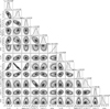 |
Fig. B.1 Corner plot for the MCMC sampling toward position 1 in Fig. 4 as a typical example. We note the 10th column represent the relative velocity between the layer 1 (front) and the layer 2 (rear). |
 |
Fig. B.2 Left: The ΔAIC map between the one-layer and two-layer models. The color contours show the area where the two-layer model is selected and the colors indicate the kinematic components II-VI (I is the main component covering the whole map; see Fig. 6). Middle: Difference of evidences between the two-layer and the one-layer models toward the points with nested sampling overlaid on continuum image. The colors and sizes represent the difference. Right: The relative velocity, i.e., the velocity difference VLSR,2 − VLSR,1 of the layer one (front layer, τ1(υ)) and layer two (rear layer, τ2(υ)) in Eq. A.5, in the two-layer model. |
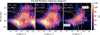 |
Fig. C.1 PV diagram of three selected transitions from CH3CN across VLA4A and VLA4B (west to east). The contour levels are at 5, 10, 15, and 20σ. The dashed lines indicate the position and velocity of VLA4A (blue) and VLA4B (orange). The solid curves show Keplerian profiles for each with a Mstar = 0.27M⊙ and θinc = 22° for VLA4A (blue) and Mstar = 0.60M⊙ and θinc = 40° for VLA4B (orange) according to Diaz-Rodriguez et al. (2022). |
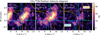 |
Fig. C.2 Same from Fig. C.1 but for CH313CN with a contour levels of 3, 5, 7, and 10σ. To improve the S/N for the CH313CN, the data is smoothed along the spectral axis. |
References
- Ahmadi, A., Beuther, H., Bosco, F., et al. 2023, A&A, 677, A171 [NASA ADS] [CrossRef] [EDP Sciences] [Google Scholar]
- Alves, F. O., Cleeves, L. I., Girart, J. M., et al. 2020, ApJ, 904, L6 [NASA ADS] [CrossRef] [Google Scholar]
- Anglada, G., Rodríguez, L. F., Osorio, M., et al. 2004, ApJ, 605, L137 [Google Scholar]
- Astropy Collaboration (Robitaille, T. P., et al.) 2013, A&A, 558, A33 [NASA ADS] [CrossRef] [EDP Sciences] [Google Scholar]
- Astropy Collaboration (Price-Whelan, A. M., et al.) 2022, ApJ, 935, 167 [NASA ADS] [CrossRef] [Google Scholar]
- Belloche, A., Maury, A. J., Maret, S., et al. 2020, A&A, 635, A198 [NASA ADS] [CrossRef] [EDP Sciences] [Google Scholar]
- Bergin, E. A., Bosman, A., Teague, R., et al. 2024, ApJ, 965, 147 [NASA ADS] [CrossRef] [Google Scholar]
- Bergner, J. B., Guzmán, V. G., Öberg, K. I., Loomis, R. A., & Pegues, J. 2018, ApJ, 857, 69 [Google Scholar]
- Bianchi, E., Codella, C., Ceccarelli, C., et al. 2017, MNRAS, 467, 3011 [NASA ADS] [CrossRef] [Google Scholar]
- Bianchi, E., Codella, C., Ceccarelli, C., et al. 2019, MNRAS, 483, 1850 [Google Scholar]
- Bianchi, E., Ceccarelli, C., Codella, C., et al. 2022a, A&A, 662, A103 [NASA ADS] [CrossRef] [EDP Sciences] [Google Scholar]
- Bianchi, E., López-Sepulcre, A., Ceccarelli, C., et al. 2022b, ApJ, 928, L3 [NASA ADS] [CrossRef] [Google Scholar]
- Birnstiel, T., Dullemond, C. P., Zhu, Z., et al. 2018, ApJ, 869, L45 [CrossRef] [Google Scholar]
- Bisschop, S. E., Jørgensen, J. K., Bourke, T. L., Bottinelli, S., & van Dishoeck, E. F. 2008, A&A, 488, 959 [NASA ADS] [CrossRef] [EDP Sciences] [Google Scholar]
- Boley, A. C., & Durisen, R. H. 2008, ApJ, 685, 1193 [Google Scholar]
- Bosman, A. D., Bergin, E. A., Loomis, R. A., et al. 2021, ApJS, 257, 15 [NASA ADS] [CrossRef] [Google Scholar]
- Bottinelli, S., Ceccarelli, C., Williams, J. P., & Lefloch, B. 2007, A&A, 463, 601 [NASA ADS] [CrossRef] [EDP Sciences] [Google Scholar]
- Cabedo, V., Maury, A., Girart, J. M., & Padovani, M. 2021, A&A, 653, A166 [NASA ADS] [CrossRef] [EDP Sciences] [Google Scholar]
- Calcutt, H., Jørgensen, J. K., Müller, H. S. P., et al. 2018, A&A, 616, A90 [NASA ADS] [CrossRef] [EDP Sciences] [Google Scholar]
- CASA Team, Bean, B., Bhatnagar, S., et al. 2022, PASP, 134, 114501 [NASA ADS] [CrossRef] [Google Scholar]
- Ceccarelli, C. 2004, ASP Conf. Ser., 323, 195 [Google Scholar]
- De Vries, C. H., & Myers, P. C. 2005, ApJ, 620, 800 [NASA ADS] [CrossRef] [Google Scholar]
- Diaz-Rodriguez, A. K., Anglada, G., Blázquez-Calero, G., et al. 2022, ApJ, 930, 91 [NASA ADS] [CrossRef] [Google Scholar]
- Di Francesco, J., Myers, P. C., Wilner, D. J., Ohashi, N., & Mardones, D. 2001, ApJ, 562, 770 [NASA ADS] [CrossRef] [Google Scholar]
- Ediss, G. A., Carter, M., Cheng, J., et al. 2004, in Fifteenth International Symposium on Space Terahertz Technology, ed. G. Narayanan (USA: NASA), 181 [Google Scholar]
- Emprechtinger, M., Caselli, P., Volgenau, N. H., Stutzki, J., & Wiedner, M. C. 2009, A&A, 493, 89 [NASA ADS] [CrossRef] [EDP Sciences] [Google Scholar]
- Endres, C. P., Schlemmer, S., Schilke, P., Stutzki, J., & Müller, H. S. P. 2016, J. Mol. Spectr., 327, 95 [NASA ADS] [CrossRef] [Google Scholar]
- Ester, M., Kriegel, H.-P., Sander, J., & Xu, X. 1996, in Second International Conference on Knowledge Discovery and Data Mining (KDD’96). Proceedings of a conference held August 2-4, eds. D. W. Pfitzner, & J. K. Salmon, 226 [Google Scholar]
- Flores, C., Ohashi, N., Tobin, J. J., et al. 2023, ApJ, 958, 98 [NASA ADS] [CrossRef] [Google Scholar]
- Galván-Madrid, R., Liu, H. B., Izquierdo, A. F., et al. 2018, ApJ, 868, 39 [CrossRef] [Google Scholar]
- Garrod, R. T., & Herbst, E. 2006, A&A, 457, 927 [NASA ADS] [CrossRef] [EDP Sciences] [Google Scholar]
- Garufi, A., Dominik, C., Ginski, C., et al. 2022, A&A, 658, A137 [NASA ADS] [CrossRef] [EDP Sciences] [Google Scholar]
- Gieser, C., Pineda, J. E., Segura-Cox, D. M., et al. 2024, A&A, 692, A55 [NASA ADS] [CrossRef] [EDP Sciences] [Google Scholar]
- Ginski, C., Facchini, S., Huang, J., et al. 2021, ApJ, 908, L25 [NASA ADS] [CrossRef] [Google Scholar]
- Goldreich, P., & Kwan, J. 1974, ApJ, 189, 441 [CrossRef] [Google Scholar]
- Gupta, A., Miotello, A., Williams, J. P., et al. 2024, A&A, 683, A133 [NASA ADS] [CrossRef] [EDP Sciences] [Google Scholar]
- Hsieh, T.-H., Lai, S.-P., Belloche, A., Wyrowski, F., & Hung, C.-L. 2015, ApJ, 802, 126 [NASA ADS] [CrossRef] [Google Scholar]
- Hsieh, T.-H., Murillo, N. M., Belloche, A., et al. 2018, ApJ, 854, 15 [NASA ADS] [CrossRef] [Google Scholar]
- Hsieh, T.-H., Murillo, N. M., Belloche, A., et al. 2019, ApJ, 884, 149 [Google Scholar]
- Hsieh, T. H., Segura-Cox, D. M., Pineda, J. E., et al. 2023, A&A, 669, A137 [NASA ADS] [CrossRef] [EDP Sciences] [Google Scholar]
- Hsieh, T. H., Pineda, J. E., Segura-Cox, D. M., et al. 2024, A&A, 686, A289 [NASA ADS] [CrossRef] [EDP Sciences] [Google Scholar]
- Hunter, J. D. 2007, Comput. Sci. Eng., 9, 90 [NASA ADS] [CrossRef] [Google Scholar]
- Jørgensen, J. K., Kuruwita, R. L., Harsono, D., et al. 2022, Nature, 606, 272 [CrossRef] [Google Scholar]
- Kang, S.-J., & Kerton, C. R. 2012, ApJ, 759, 13 [Google Scholar]
- Koposov, S., Speagle, J., Barbary, K., et al. 2022, https://doi.org/10.5281/zenodo.7388523 [Google Scholar]
- Kuffmeier, M., Haugbølle, T., & Nordlund, Å. 2017, ApJ, 846, 7 [NASA ADS] [CrossRef] [Google Scholar]
- Lee, C. W., Myers, P. C., & Tafalla, M. 2001, ApJS, 136, 703 [NASA ADS] [CrossRef] [Google Scholar]
- Lee, J.-E., Lee, S., Baek, G., et al. 2019, Nat. Astron., 3, 314 [Google Scholar]
- Loomis, R. A., Cleeves, L. I., Öberg, K. I., et al. 2018, ApJ, 859, 131 [Google Scholar]
- Machida, M. N., Inutsuka, S.-I., & Matsumoto, T. 2011, ApJ, 729, 42 [NASA ADS] [CrossRef] [Google Scholar]
- Mardones, D., Myers, P. C., Tafalla, M., et al. 1997, ApJ, 489, 719 [Google Scholar]
- Maureira, M. J., Gong, M., Pineda, J. E., et al. 2022, ApJ, 941, L23 [NASA ADS] [CrossRef] [Google Scholar]
- Milam, S. N., Savage, C., Brewster, M. A., Ziurys, L. M., & Wyckoff, S. 2005, ApJ, 634, 1126 [Google Scholar]
- Möller, T., Endres, C., & Schilke, P. 2017, A&A, 598, A7 [NASA ADS] [CrossRef] [EDP Sciences] [Google Scholar]
- Müller, H. S. P., Schlöder, F., Stutzki, J., & Winnewisser, G. 2005, J. Mol. Struc., 742, 215 [Google Scholar]
- Müller, H. S. P., Drouin, B. J., & Pearson, J. C. 2009, A&A, 506, 1487 [NASA ADS] [CrossRef] [EDP Sciences] [Google Scholar]
- Müller, H. S. P., Brown, L. R., Drouin, B. J., et al. 2015, J. Mol. Spectr., 312, 22 [CrossRef] [Google Scholar]
- Murillo, N. M., Hsieh, T. H., & Walsh, C. 2022a, A&A, 665, A68 [NASA ADS] [CrossRef] [EDP Sciences] [Google Scholar]
- Murillo, N. M., van Dishoeck, E. F., Hacar, A., Harsono, D., & Jørgensen, J. K. 2022b, A&A, 658, A53 [NASA ADS] [CrossRef] [EDP Sciences] [Google Scholar]
- Murillo, N. M., Fuchs, C. M., Harsono, D., et al. 2024, A&A, 689, A267 [NASA ADS] [CrossRef] [EDP Sciences] [Google Scholar]
- Myers, P. C., Mardones, D., Tafalla, M., Williams, J. P., & Wilner, D. J. 1996, ApJ, 465, L133 [NASA ADS] [CrossRef] [Google Scholar]
- Öberg, K. I., Garrod, R. T., van Dishoeck, E. F., & Linnartz, H. 2009, A&A, 504, 891 [NASA ADS] [CrossRef] [EDP Sciences] [Google Scholar]
- Offner, S. S. R., Klein, R. I., McKee, C. F., & Krumholz, M. R. 2009, ApJ, 703, 131 [CrossRef] [Google Scholar]
- Offner, S. S. R., Moe, M., Kratter, K. M., et al. 2023, ASP Conf. Ser., 534, 275 [NASA ADS] [Google Scholar]
- Ortiz-León, G. N., Loinard, L., Dzib, S. A., et al. 2018, ApJ, 865, 73 [Google Scholar]
- Ossenkopf, V., & Henning, T. 1994, A&A, 291, 943 [NASA ADS] [Google Scholar]
- Pickett, H. M., Poynter, R. L., Cohen, E. A., et al. 1998, J. Quant. Spec. Radiat. Transf., 60, 883 [Google Scholar]
- Pineda, J. E., Maury, A. J., Fuller, G. A., et al. 2012, A&A, 544, L7 [NASA ADS] [CrossRef] [EDP Sciences] [Google Scholar]
- Pineda, J. E., Segura-Cox, D., Caselli, P., et al. 2020, Nat. Astron., 4, 1158 [NASA ADS] [CrossRef] [Google Scholar]
- Pineda, J. E., Arzoumanian, D., Andre, P., et al. 2023, ASP Conf. Ser., 534, 233 [NASA ADS] [Google Scholar]
- Podio, L., Ceccarelli, C., Codella, C., et al. 2024, A&A, 688, L22 [NASA ADS] [CrossRef] [EDP Sciences] [Google Scholar]
- Rab, C., Elbakyan, V., Vorobyov, E., et al. 2017, A&A, 604, A15 [NASA ADS] [CrossRef] [EDP Sciences] [Google Scholar]
- Redaelli, E., Chacón-Tanarro, A., Caselli, P., et al. 2022, ApJ, 941, 168 [NASA ADS] [CrossRef] [Google Scholar]
- Rosotti, G. P., Ilee, J. D., Facchini, S., et al. 2021, MNRAS, 501, 3427 [Google Scholar]
- Sahu, D., Liu, S.-Y., Su, Y.-N., et al. 2019, ApJ, 872, 196 [Google Scholar]
- Sánchez-Monge, Á., Schilke, P., Ginsburg, A., Cesaroni, R., & Schmiedeke, A. 2018, A&A, 609, A101 [Google Scholar]
- Segura-Cox, D. M., Looney, L. W., Tobin, J. J., et al. 2018, ApJ, 866, 161 [Google Scholar]
- Shu, F. H. 1977, ApJ, 214, 488 [Google Scholar]
- Skilling, J. 2004, AIP Conf. Ser., 735, 395 [Google Scholar]
- Sokolov, V., Pineda, J. E., Buchner, J., & Caselli, P. 2020, ApJ, 892, L32 [NASA ADS] [CrossRef] [Google Scholar]
- Speagle, J. S. 2020, MNRAS, 493, 3132 [Google Scholar]
- Tafalla, M., Mardones, D., Myers, P. C., et al. 1998, ApJ, 504, 900 [NASA ADS] [CrossRef] [Google Scholar]
- Terebey, S., Shu, F. H., & Cassen, P. 1984, ApJ, 286, 529 [Google Scholar]
- Thieme, T. J., Lai, S.-P., Lin, S.-J., et al. 2022, ApJ, 925, 32 [NASA ADS] [CrossRef] [Google Scholar]
- Tobin, J. J., Looney, L. W., Li, Z.-Y., et al. 2018, ApJ, 867, 43 [CrossRef] [Google Scholar]
- Tokovinin, A. 2014, AJ, 147, 87 [CrossRef] [Google Scholar]
- Toomre, A. 1964, ApJ, 139, 1217 [Google Scholar]
- Valdivia-Mena, M. T., Pineda, J. E., Segura-Cox, D. M., et al. 2022, A&A, 667, A12 [NASA ADS] [CrossRef] [EDP Sciences] [Google Scholar]
- Valdivia-Mena, M. T., Pineda, J. E., Segura-Cox, D. M., et al. 2023, A&A, 677, A92 [NASA ADS] [CrossRef] [EDP Sciences] [Google Scholar]
- Valdivia-Mena, M. T., Pineda, J. E., Caselli, P., et al. 2024, A&A, 687, A71 [NASA ADS] [CrossRef] [EDP Sciences] [Google Scholar]
- van der Walt, S., Colbert, S. C., & Varoquaux, G. 2011, Comput. Sci. Eng., 13, 22 [Google Scholar]
- Vastel, C., Bottinelli, S., Caux, E., Glorian, J. M., & Boiziot, M. 2015, in SF2A- 2015: Proceedings of the Annual meeting of the French Society of Astronomy and Astrophysics, 313 [Google Scholar]
- Virtanen, P., Gommers, R., Burovski, E., et al. 2020, Scipy/scipy: SciPy 1.5.3 [Google Scholar]
- Vorobyov, E. I., & Basu, S. 2005, ApJ, 633, L137 [NASA ADS] [CrossRef] [Google Scholar]
- Vorobyov, E. I., & Basu, S. 2010, ApJ, 719, 1896 [NASA ADS] [CrossRef] [Google Scholar]
- Yamato, Y., Notsu, S., Aikawa, Y., et al. 2024, AJ, 167, 66 [NASA ADS] [CrossRef] [Google Scholar]
- Yang, Y.-L., Sakai, N., Zhang, Y., et al. 2021, ApJ, 910, 20 [Google Scholar]
- Yen, H.-W., Gu, P.-G., Hirano, N., et al. 2019, ApJ, 880, 69 [NASA ADS] [CrossRef] [Google Scholar]
- Yoshida, T. C., Nomura, H., Furuya, K., Tsukagoshi, T., & Lee, S. 2022, ApJ, 932, 126 [NASA ADS] [CrossRef] [Google Scholar]
- Yoshida, T. C., Nomura, H., Furuya, K., et al. 2024, ApJ, 966, 63 [Google Scholar]
All Tables
All Figures
|
Fig. 1 Left: integrated intensity map of the CH3CN J=12-11 K=3 ladder with the contours from 1.3 mm continuum at levels of 3, 5, 7, 10, 20, 40, 100, and 200σ, with σ = 0.2 K. Right: sSpectra seen from the cross-marked positions of VLA4A (top) and VLA4B (bottom) from the CH3CN window. The red lines represent the best fits from our models (see Sects. 4.2.1 and 4.2.2). |
| In the text | |
|
Fig. 2 Integrated intensity map of the CH3CN J=12-11 with K=0, 3, and 7. The integration range is 4–12 km s−1. The contours represent the 1.3 mm continuum emission at levels of 3, 5, 10, 20, 50, 150, and 300σ with σ =0.2 K. The blue cross markers indicate the locations of VLA4A and VLA4B from the continuum emission. |
| In the text | |
|
Fig. 3 Same as Fig. 2, but for the integrated intensity map of the CH313CN J=12-11 with k=1, 2, and 5. The integration range is 5.5–11 km s−1 . |
| In the text | |
|
Fig. 4 Spectra of CH3CN toward SVS13A at selected positions marked in the central image of the K=3 integrated intensity map. In the central image, the white contours represent the S/N of 3 and 12, as the latter represents the region where LTE fitting is made. The blue stars indicate the positions of VLA4A and VLA4B. The kinematic components II-VI (II: red, III: green, IV: orange, V:purple, VI: yellow; see Fig. 6) are shown as contours in different colors and for the positions within a contour, the two-layer LTE model is used for fitting (see Sect. 4.3). Each spectrum has been divided to eight individual panels centering at the Vlsr, i.e., 7.36 km s−1 for VLA4A and 9.33 km s−1 for VLA4B (Diaz-Rodriguez et al. 2022 blue and red dashed vertical lines in the K=0 panel), of the K-ladder. The red spectra show the best-fit from the LTE model while the color areas show the two-layer model with front (1, orange) and rear (2, purple) layers. We note that Eq. (2) is more complicated, so this colored area is only meant to offer an general view of Vlsr and ∆V. |
| In the text | |
|
Fig. 5 Fitting results of the one-layer LTE model. Each panel shows a map of the free parameter with the label of the colorbar on the top. The contours on the first panel represents the 1.3 mm continuum emission (Fig. 2). The contours of the second column represents τ at 1 and 2, while those in the sixth column show the isotopolog ratios of 15 and 68. The fourth column gives the Vlsr map, where the systemic velocities of VLA4A and VLA4B are 7.36 and 9.33 km s−1, respectively (Diaz-Rodriguez et al. 2022). |
| In the text | |
|
Fig. 6 PPV diagram from the combination of one- and two-layer model fitting. The bottom x-y image is the CH3CN J=12-11 K=3 integrated intensity map. Above it, each position can have one or two velocities. The color of data points indicates the kinematic component from clustering. The two cyan vertical lines indicates the positions and the systemic velocities of VLA4A (7.36 km s−1) and VLA4B (9.33 km s−1). |
| In the text | |
|
Fig. 7 Absolute relative velocity of the component II-VI with respect to the main component I. The contours represent the continuum emission with the same levels as Fig. 1. The color contours show the area of component II-VI. |
| In the text | |
|
Fig. 8 Same as Fig. 5, but for the clustering components. Note: the discarded points are attributed to one-layer fitting in component I. The top, middle, and bottom panels show the parameters for component I, II, and III-VI, respectively. The fourth column shows the Vlsr map, with the systemic velocities of VLA4A and VLA4B calculated as 7.36 and 9.33 km s−1, respectively (Diaz-Rodriguez et al. 2022). |
| In the text | |
|
Fig. 9 Left column: velocity map of component I (Fig. 8) relative to VLA4A (top, VVLA4A = 7.36 km s−1) and VLA4B (bottom, VVLA4B = 9.33 km s−1). Middle: Keplerian disk model using the Mstar and θinc from Diaz-Rodriguez et al. (2022). We note that the inclination angle of VLA4B is from the dust continuum as the gas disk is not seen here. Right: Toomre Q map derived using the physical parameters from CH3CN plus models of rotation from the middle panel. |
| In the text | |
|
Fig. B.1 Corner plot for the MCMC sampling toward position 1 in Fig. 4 as a typical example. We note the 10th column represent the relative velocity between the layer 1 (front) and the layer 2 (rear). |
| In the text | |
|
Fig. B.2 Left: The ΔAIC map between the one-layer and two-layer models. The color contours show the area where the two-layer model is selected and the colors indicate the kinematic components II-VI (I is the main component covering the whole map; see Fig. 6). Middle: Difference of evidences between the two-layer and the one-layer models toward the points with nested sampling overlaid on continuum image. The colors and sizes represent the difference. Right: The relative velocity, i.e., the velocity difference VLSR,2 − VLSR,1 of the layer one (front layer, τ1(υ)) and layer two (rear layer, τ2(υ)) in Eq. A.5, in the two-layer model. |
| In the text | |
|
Fig. C.1 PV diagram of three selected transitions from CH3CN across VLA4A and VLA4B (west to east). The contour levels are at 5, 10, 15, and 20σ. The dashed lines indicate the position and velocity of VLA4A (blue) and VLA4B (orange). The solid curves show Keplerian profiles for each with a Mstar = 0.27M⊙ and θinc = 22° for VLA4A (blue) and Mstar = 0.60M⊙ and θinc = 40° for VLA4B (orange) according to Diaz-Rodriguez et al. (2022). |
| In the text | |
|
Fig. C.2 Same from Fig. C.1 but for CH313CN with a contour levels of 3, 5, 7, and 10σ. To improve the S/N for the CH313CN, the data is smoothed along the spectral axis. |
| In the text | |
Current usage metrics show cumulative count of Article Views (full-text article views including HTML views, PDF and ePub downloads, according to the available data) and Abstracts Views on Vision4Press platform.
Data correspond to usage on the plateform after 2015. The current usage metrics is available 48-96 hours after online publication and is updated daily on week days.
Initial download of the metrics may take a while.