| Issue |
A&A
Volume 686, June 2024
|
|
|---|---|---|
| Article Number | A289 | |
| Number of page(s) | 25 | |
| Section | Interstellar and circumstellar matter | |
| DOI | https://doi.org/10.1051/0004-6361/202449417 | |
| Published online | 24 June 2024 | |
PRODIGE – envelope to disk with NOEMA
III. The origin of complex organic molecule emission in SVS13A★
1
Max-Planck-Institut für extraterrestrische Physik,
Giessenbachstrasse 1,
85748
Garching, Germany
e-mail: This email address is being protected from spambots. You need JavaScript enabled to view it.
2
Department of Astronomy, The University of Texas at Austin,
2500 Speedway,
Austin, TX,
78712, USA
3
Institut de Radioastronomie Millimétrique (IRAM),
300 rue de la Piscine,
38406,
Saint-Martin d’Hères, France
4
Univ. Grenoble Alpes, CNRS, IPAG,
38000
Grenoble, France
5
I. Physikalisches Institut, Universität zu Köln,
Zülpicher Str. 77,
50937
Köln, Germany
6
Laboratoire d’Astrophysique de Bordeaux, Université de Bordeaux, CNRS, B18N,
Allée Geoffroy Saint-Hilaire,
33615
Pessac, France
7
Centro de Astrobiología (CAB), CSIC-INTA,
Ctra.deTorrejón a Ajalvir km 4,
28806,
Torrejón de Ardoz, Spain
8
Max-Planck-Institut für Astronomie,
Königstuhl 17,
69117
Heidelberg, Germany
9
Department of Physics and Astronomy, University of Exeter,
Stocker Road,
Exeter,
EX4 4QL, UK
Received:
30
January
2024
Accepted:
22
March
2024
Abstract
Context. Complex organic molecules (COMs) have been found toward low-mass protostars, but the origins of the COM emission are still unclear. It can be associated with, for example, hot corinos, outflows, and/or accretion shock and disk atmospheres.
Aims. We aim to disentangle the origin of the COM emission toward the chemically rich protobinary system SVS13A using six O-bearing COMs.
Methods. We conducted NOrthern Extended Millimeter Array observations toward SVS13A as part of the PROtostars & DIsks: Global Evolution (PRODIGE) program. Our previous DCN observations reveal a possible infalling streamer, which may affect the chemistry of the central protobinary by inducing accretion outbursts and/or shocked gas. We further analyzed six O-bearing COMs: CH3OH, aGg’- (CH2OH)2, C2H5OH, CH2(OH)CHO, CH3CHO, and CH3OCHO. Although the COM emission is not spatially resolved, we constrained the source sizes to ≲0.3–0.4 arcsec (90–120 au) by conducting uv-domain Gaussian fitting. Interestingly, the high-spectral-resolution data reveal complex line profiles with multiple peaks; although the line emission is likely dominated by the secondary, VLA4A, at VLSR = 7.36 km s−1, the numbers of peaks (~2–5), the velocities, and the linewidths of these six O-bearing COMs are different. The local thermodynamic equilibrium (LTE) fitting unveils differences in excitation temperatures and emitting areas among these COMs. We further conducted multiple-velocity-component LTE fitting to decompose the line emission into different kinematic components. As a result, the emission of these COMs is decomposed into up to six velocity components from the LTE modeling. The physical conditions (temperature, column density, and source size) of these components from each COM are obtained, and Markov chain Monte Carlo sampling was performed to test the fitting results.
Results. We find a variety in excitation temperatures (100–500 K) and source sizes (D ~ 10–70 au) from these kinematic components from different COMs. The emission of each COM can trace several components, and different COMs most likely trace different regions.
Conclusions. Given this complex structure, we suggest that the central region is inhomogeneous and unlikely to be heated by only protostellar radiation. We conclude that accretion shocks induced by the large-scale infalling streamer likely exist and contribute to the complexity of the COM emission. This underlines the importance of high-spectral-resolution data when analyzing COM emission in protostars and deriving relative COM abundances.
Key words: line: formation / radiative transfer / ISM: kinematics and dynamics / ISM: molecules
Based on observations carried out under project number L19MB with the IRAM NOEMA Interferometer. IRAM is supported by INSU/CNRS (France), MPG (Germany), and IGN (Spain).
NSF Astronomy and Astrophysics Postdoctoral Fellow.
© The Authors 2024
 Open Access article, published by EDP Sciences, under the terms of the Creative Commons Attribution License (https://creativecommons.org/licenses/by/4.0), which permits unrestricted use, distribution, and reproduction in any medium, provided the original work is properly cited.
This article is published in open access under the Subscribe to Open model.
Open Access funding provided by Max Planck Society.
1 Introduction
About 270 molecules have been found in the interstellar medium so far (Ceccarelli et al. 2022). Of these molecules, 40% are so-called interstellar complex organic molecules (COMs), defined as carbon-bearing molecules that have at least six atoms (Herbst & van Dishoeck 2009; Ceccarelli et al. 2017). COMs are commonly detected in massive star-forming regions (Blake et al. 1987; Gieser et al. 2023) and are also occasionally detected toward solar-type protostellar systems (Caselli & Ceccarelli 2012; van Dishoeck 2014, and references therein). In Class 0 pro- tostars, COMs are seen in several cases, including IRAS 16293-2422 (van Dishoeck et al. 1995; Cazaux et al. 2003; Jørgensen et al. 2018), NGC 1333-IRAS 4A (Cazaux et al. 2003), and NGC 1333-IRAS 4B/IRAS2A (Bottinelli et al. 2007). COMs have even been detected toward pre-stellar cores (e.g., L1689B: Bacmann et al. 2012, L1544: Tafalla et al. 2006; Spezzano et al. 2016). Despite the wide variety of COMs and the types of objects in which they are found, we still have not yet fully characterized the origins of COM emission observationally.
In low-mass star-forming regions, COMs in the ice man- tles of dust grains can sublimate into the gas phase in regions heated by the central protostars (>100 K). This zone is named the “hot corino”, a compact source (≲100 au) with high tem- peratures (>100 K) and high densities (>107 cm−3; Caselli & Ceccarelli 2012; Ceccarelli et al. 2022). COMs are also found toward outflow cavity walls believed to be induced by shocks or protostellar UV irradiation (Jørgensen et al. 2004; Arce et al. 2008; Sugimura et al. 2011; Drozdovskaya et al. 2015; Palau et al. 2017). Furthermore, Oya et al. (2016) propose that at the centrifu- gal radius where the infalling material from the envelope lands on a protostellar disk, COMs can be liberated from dust man- tles by weak accretion shocks in IRAS 16293-2422A. Similar scenarios are suggested by recent observations by Codella et al. (2018) and Vastel et al. (2022) toward HH212 and BHB2007 11, respectively. Belloche et al. (2020) categorized the COM emis- sion in low-mass protostars into three groups: (1) hot corinos, (2) outflows, and (3) accretion shock and disk atmospheres.
Complex organic molecules are known to arise from SVS13A (Bianchi et al. 2017, 2019, 2022a,b; Lefloch et al. 2018; Belloche et al. 2020; Yang et al. 2021; Diaz-Rodriguez et al. 2022), a Class I protobinary system located in the NGC 1333 cluster within the Perseus Molecular Cloud (d = 293 pc; Ortiz-León et al. 2018). SVS13A contains two protostars, VLA4A and VLA4B, with a projected distance of 0.″3 (~90 au) based on the continuum observations (see the first panel of our Fig. 1 as well as Anglada et al. 2004; Tobin et al. 2016, 2018; Segura-Cox et al. 2018; Tychoniec et al. 2020). From multi-epoch observations, Diaz-Rodriguez et al. (2022) derived the total mass of the binary to be 1.0+0.4 M⊙ using orbital motions (see also Maureira et al. 2020). By modeling the kinematics of the line emission, they further estimate stel- lar masses of 0.27±0.10 M⊙ for VLA4A and 0.60±0.20 M⊙ for VLA4B. The existence of a third hidden source at a dis- tance of ~20–30 au from VLA4B is implied by the wiggling jets seen at large scales (Lefèvre et al. 2017). At least two spi- rals have been identified from the dust continuum emission (Diaz-Rodriguez et al. 2022), and they had been considered to be part of a fragmenting disk due to gravitational instability (Tobin et al. 2018). However, recent observations find that the dust spiral is connected to a larger-scale structure (at least 700 au) through a streamer traced by DCN emission, which perhaps delivers mate- rial from the envelope to the central system (Hsieh et al. 2023). Such infalling streamers at envelope scales have recently been identified toward several protostellar systems, which are sug- gested to funnel material near or into smaller-scale disks (Pineda et al. 2020, 2023; Alves et al. 2020; Ginski et al. 2021; Murillo et al. 2022; Cabedo et al. 2021; Garufi et al. 2022; Thieme et al. 2022; Valdivia-Mena et al. 2022). These infalling flows are believed to change the chemistry of the inner region (disk and/or inner envelope) by directly funneling material, induc- ing shock gas, and/or indirectly triggering protostellar outbursts. For SVS13A, the high luminosity, Lbol = 45.3 L⊙, suggests that it is undergoing a protostellar accretion outburst. This makes SVS13A a good candidate for studying the chemical inventory under the influence of an accretion burst.
In this paper we present new NOrthern Extended Mil- limeter Array (NOEMA) data at 1.3 mm toward SVS13A. We selected six oxygen-bearing (O-bearing) COMs (CH3OH, aGg’-(CH2OH)2, C2H5OH, CH2(OH)CHO, CH3CHO, and CH3OCHO) that are found to be relatively bright with com- plex line profiles (multiple peaks) in our data; O-bearing COMs are also suggested to be more abundant relative to CH3OH in shock regions (Csengeri et al. 2018, 2019). CH3OCH3 is also detected but in only a few blended transitions, preventing a detailed kinematic analysis (Appendix C). This work focuses on disentangling the kinematics of the protostellar system to deter- mine from which structures the COM emission originates, taking advantage of the high spectral resolution and broadband capabil- ities of the Institut de Radioastronomie Millimétrique (IRAM) NOEMA PolyFiX correlator. In Sect. 2 we describe the obser- vations and calibration. The results are presented in Sect. 3. In Sect. 4 we detail the analysis, and we discuss our findings in Sect. 5. Our conclusions are summarized in Sect. 6.
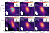 |
Fig. 1 Integrated intensity maps of a selected transition for each O-bearing COM. The top-right panel in each figure shows the spectra toward the center, and the filled regions indicate the integration range for the zero-order moment maps, which is 3.5–10.7 km s−1 (except for CH3OH, for which it is 3.5–12.0 km s−1), for the zero-order moment maps. The blue contours in the top-left panel represent the ALMA 1.3 mm continuum emission (Tobin et al. 2018) with levels of [3, 5, 7, 10, 30, 70]σ. The horizontal gray line in the top-left panel shows the PV cut used in Fig. 7. The blue pixel in the top-right panel is the pixel used to extract the spectra in this work. |
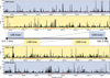 |
Fig. 2 Low-spectral-resolution spectrum toward the continuum peak of SVS13A from the PRODIGE NOEMA large program. The panels, from top to bottom, represent the spectra from the receiver bands as shown in the sketch in the middle. The horizontal orange bars represent locations of the high-spectral-resolution windows. |
2 Observations
The observations were carried out with NOEMA at IRAM. It is part of the MPG-IRAM observing program PROtostars & DIsks: Global Evolution (PRODIGE; Project ID: L19MB002, PIs: P. Caselli and Th. Henning). The observations are briefly described in Hsieh et al. (2023) that reports the data of  , DCN J = 3–2, and CH3CN J = 12k−11k (K = 0–7).
In this paper we present the data covering six O-bearing COMs: CH3OH, aGg’-(CH2OH)2 (the most stable conformer of (CH2OH)2, Christen et al. 2001), C2H5OH, CH2(OH)CHO, CH3CHO, and CH3OCHO. Here we describe the receiver setups with the PolyFiX correlator. The receiver contains four broad- band dual polarization low-resolution windows and 39 narrow- band high-resolution windows. The broadband windows cover 214.7–218.8 GHz, 218.8–222.8 GHz, 230.2–234.2 GHz, and 234.2–238.3 GHz with a channel width of 2 MHz (~2.7 km s−1). The 39 narrowband windows are distributed within the men- tioned ranges with a channel width of 62.5 kHz (Fig. 2). The resulting spectral resolutions of the narrowband windows are ~0.078–0.086 km s−1.
Self-calibration was performed with solution intervals of 300, 135, and 45 s on the broadband data as in Hsieh et al. (2023). The solutions are then applied to the broadband and nar- rowband data. Imaging was done using the GILDAS/MAPPING package1. We used the clean task with natural weighting in order to get the best sensitivity. This gives beam sizes of 1.″11 × 0.″67 to 1.″24 × 0.″73 with a rms noise level of ~0.5 K at a resolution of ~0.8 km s–1. Given the large number of channels in both the broadband data and the high-spectral-resolution datasets, we did not clean using a support mask, and a shallow clean of the whole image with a 5σ threshold was performed, where σ is the rms noise level. The single-point spec- tra toward the continuum peak (pixel at α = 3h29m 03s.75, δ = 31d16m03s.73) were extracted for analysis.
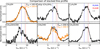 |
Fig. 3 Comparison of stacked line profiles of the six O-bearing COMs. The stacking was done using spectra normalized to their peak fluxes and weighting with the reciprocal of noise squared (Appendix A). The vertical dashed lines indicate the central velocities of the disks of VLA4A (blue), 4B (red), and the circumbinary disk (gray) from Diaz-Rodriguez et al. (2022). |
3 Results
3.1 Line identification
Figure 2 shows the full NOEMA spectrum from the broadband low-resolution data toward the continuum peak. Line identifica- tion is first conducted using the Lineldentification function of the eXtended CASA Line Analysis Software Suite (XCLASS) package, which automatically identifies lines, derives a quan- titative description of each identified species, and return the corresponding physical parameters including the temperature, column density, source size, linewidth and systemic velocity (XCLASS, Möller et al. 2017) with the full broadband windows covering 16 GHz. We disentangle the complicated line profiles using high-spectral-resolution data in a later section.
3.2 Stacking of lines
In order to increase the signal of the multiple peak structures, we stacked the spectra from selected transitions for each COM; we manually selected several transitions that are less contam- inated by others. To be selected, the transition is expected to be broadly consistent with the XCLASS modeling result in amplitudes and share similar linewidths and spectral profiles (Sect. 3.1). Columns 7 in Tables B.1 to B.6 list the transitions that were stacked (see Appendix A and Fig. A.1). The spectra were first interpolated to the same grid using the SciPy package (Virtanen et al. 2020). The spectra were then normalized by the peak flux and averaged with a weight of the inverse of square noise (σ′; i.e., the noise after normalization) using NumPy (Van Der Walt et al. 2011):
 (1)
(1)
The stacked line profiles help confirm multiple peaks in com- plex line profiles; we note that these lines have different opacities and energy levels, so their profiles are not necessary the same. For CH2(OH)CHO, (CH2OH)2, and C2H5OH, there are limits of selected transitions or similar Eup in the range 40–450 K for CH2(OH)CHO, 110–266 K for aGg’-(CH2OH)2, 23–409 K for C2H5OH, and 129–207 K for CH3OCHO for CH3OCHO. The stacked profile are broadly similar to the individual spectral pro- file (Fig. A.1). For CH3OH, we split the transitions with Eup in the ranges 45–96 K and 775–802 K to stack. CH3CHO have 13 selected transitions and were split into ones with 81–128 K and ones with 287–490 K. Since the stacked line profile reveals a complex line profile, we need a model to disentangle the kinematic components from it.
Figure 3 shows the stacked line profiles for the six selected O-bearing COMs toward the continuum peak. It shows that different COMs have multiple peaks at different velocities, sug- gesting that they trace different kinematic components in the system. In comparison to the systemic velocities of VLA4A/4B and the circumbinary disks, a dip is shown roughly at the velocity of VLA4A for the selected O-bearing COMs, with the exception of CH3OH. For CH3CHO, it seems a second dip at the sys- temic velocity of the circumbinary disk. These differences also support that these molecules trace different kinematic compo- nents. These kinematic components are likely associated with the physical structures, for example, the disk, shocks, streamer, or the outflow. aGg’-(CH2OH)2 shows a double peak struc- ture likely tracing the rotating disk or envelope of VLA4A. This is consistent with the results from high-angular-resolution Atacama Large Millimeter/submillimeter Array (ALMA) obser- vations (Diaz-Rodriguez et al. 2022) that aGg’-(CH2OH)2 only traces the disk around VLA4A. A double peak profile cen- tered toward VLA4A is also seen in CH2(OH)CHO. However, CH2(OH)CHO is narrower and its blueshifted peak is brighter while the opposite is true for aGg’-(CH2OH)2. On the other hand, C2H5OH, CH3OCHO, and CH3CHO emission contains more than two peaks, which likely trace not only the VLA4A disk but also the circumbinary disk and/or VLA4B and perhaps stream- ers, shocks, inner envelopes, etc. These results are summarized in Table 1.
Notes. The contributed components based on the stacked line profiles (“spectra”; see Sect. 3.2) and uv-domain Gaussian fitting (“spatial”; see Sect. 3.4).
Emitting components based on spectra and location.
3.3 Gaussian widths and velocities
To first examine the different physical structures a molecule traces, we conducted Gaussian fitting to the line profiles (narrow- band) of each selected transition from the six O-bearing COMs. The transitions are listed in Tables B.1–B.6.
Figure 4 shows a comparison of the best-fit linewidths and the central velocities of these spectral-line profiles with a single Gaussian. Although we have a limited number of uncontaminated transitions, it is clear that the linewidths and central veloci- ties are different between the O-bearing COM species. This sug- gests that these COMs can be associated with different kinematic components in the protobinary system SVS13A. Considering the central velocities, it is likely that CH2(OH)CHO, aGg’-(CH2OH)2, and CH3CHO emission is dominated by VLA4A while CH3OH, C2H5OH, and CH3OCHO likely have signifi- cant emission coming from the circumbinary disk (and perhaps VLA4B).
3.4 Spatial distribution of COM emission
To derive properties of the gas traced by the COM emission, it is crucial to know the source size. Figure 1 shows the integrated intensity maps of the six selected O-bearing COMs. All of them show point-source like structure given the spatial resolution of ~1.″2 × 0.″7 (~300 au). The deconvolved source sizes from the uv-domain Gaussian fitting (≲0.″3, 90 au) are smaller than the beam size, suggesting that they are point sources at the current resolution. This gives an upper limit of the emitting regions of ~90 au. More discussions on the source sizes are provided in Sects. 4.1 and 4.2. The compact sources might rule out the possi- bility that the emission comes from larger-scale structures, such as irradiated cavity walls carved by the bipolar outflows.
The peak positions of line emission are used to indicate the most likely location of the emitting gas at specific velocity, espe- cially for optically thin lines (Sargent & Beckwith 1987; Harsono et al. 2013). Toward SVS13A, Hsieh et al. (2023) conducted a uv-domain Gaussian fitting to CH3CN emission using a channel width of 0.5 km s−1, and found a velocity gradient from west to east (Fig. 5, top panel); the visibility data are first resampled to a width of 0.5 km s−1, and uv_fit task in MAPPING is used to con- duct the 2D Gaussian fit for each channel. We applied the same technique to six O-bearing COMs in SVS13A with the selected transitions (From Tables B.1 to B.6). This revealed the spatial weighting centers of each velocity for each transition.
The O-bearing lines have lower S/Ns compared to the CH3CN emission, especially in the red- or blueshifted wings. For uv-plane fitting of the O-bearing COM emission, we only considered data points with S/N > 7 and position uncertainty <0.″5. Figure 5 shows the fitted central positions. It is note- worthy that, for each molecule, although the transitions have different upper energy levels and opacities (Tables B.1–B.6), the spatial distributions are similar. It is clear that the emission of these O-bearing COMs originates from different locations in the system. CH3OH, C2H5OH, and CH3OCHO show a velocity gra- dient with the direction consistent with that of CH3CN. These three molecules also share similar systemic velocity ~8.1 km s−1 from the line profile fitting (Fig. 4). However, the redshifted end of CH3OCHO extends close to VLA4B while the CH3OH is relatively compact and likely dominated by VLA4A. For aGg’-(CH2OH)2, CH2(OH)CHO, and CH3CHO, the line emis- sion most likely comes from VLA4A. This agrees with the results from line stacking except for CH3CHO, which has 3–4 components (Fig. 3). However, considering their Gaussian peak velocity, these molecules have emission dominated by VLA4A (Fig. 4). We summarize them in Table 1.
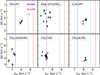 |
Fig. 4 Gaussian linewidth versus central velocity of the selected transitions from the six O-bearing COMs. The vertical dashed lines rep- resent the central velocities of the disks of VLA4A (blue), 4B (red), and the circumbinary disk (gray). The transitions in use are listed in Tables B.1–B.6. |
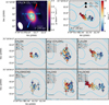 |
Fig. 5 Central positions of selected COM transitions at different velocities. The top two panels show the integrated intensity map (left) and central positions (right) from CH3CN (Hsieh et al. 2023) as a reference for the O-bearing COMs. The contours show the 1.3 mm continuum emission from Tobin et al. (2018). Different line transitions are marked with different symbols (Tables B.1-B.6). The scale bar is 0.″1 for the bottom six panels. The beam sizes for these COM emissions depend on the line frequency but are the same as that of CH3CN (1.″2 × 077) within 10%. |
4 Analysis
4.1 One-component LTE Gaussian model
We applied radiative transfer modeling to the emission of selected transitions of the six O-bearing COMs. Though multiple peaks are found in the line profiles from the high-spectral-resolution data (Fig. 3.2), we first performed local thermody- namic equilibrium (LTE) modeling of the spectra with one Gaussian velocity component. We used the LTE approach as the collisional rate coefficients of COMs are only available in a few COMs (e.g., from the Leiden Atomic and Molecular Database2). This one component model provides the first-order estimate of the physical conditions of the gas traced by each COM molecule; we use multiple Gaussian component model- ing to decompose the complex structures in Sect. 4.2. Non-LTE analysis had already been done for CH3OH (Bianchi et al. 2017:  ) and CH3CN (Hsieh et al. 2023:
  and
and  with two components). These analyses, for the only two COMs with known collision coefficients, suggest that COMs come from the central dense regions, implying that LTE analysis is reasonable for other COMs.
We applied the model to fit the high-spectral-resolution spec- tra extracted from the position of the peak continuum emission. The NOEMA observations at 1.3 mm cover ~200–1400 transi- tions, depending on the species (Fig. 2). At the same time, line contamination from nearby transitions becomes a severe issue to model the line profiles (Fig. 2). We therefore checked the line profiles from all transitions covered in the high-spectral-resolution data for each molecule. We selected as many transi- tions as possible with a range of line strengths and upper energy levels to better constrain the physical conditions (Tables B.1–B.6). The selection process is done by iteratively checking the model and line profiles of all transitions located in the narrow band windows. Based on the XCLASS model (Sect. 3.1, fit- ting the low-spectral-resolution data with the latest and most complete list of molecules), a transition that is contaminated by different molecules is first removed. A line emission much higher than the model profile may be also considered as contaminated by unidentified lines. In the other word, the final (one-velocity-component) model of the high-spectral-resolution data is broadly consistent with the XCLASS model considering more channels but fewer transitions. Line contamination can also be treated by masking the specific, overlapping velocity ranges so that more transitions can be included (Figs. B.1–B.6). Unlike line stacking (Sect. 3.2), the fit includes line profiles with several overlap- ping transitions from the same molecule (see below). In addition, undetected transitions can be included as they help constrain the physical conditions, especially when the transition has a high Einstein coefficient and/or low upper energy level.
We constructed a LTE-radiative transfer model to fit the line profiles of the selected transitions. The model includes five free parameters: column density (Ntot), excitation temperature (Tex), central velocity (VLSR), linewidth (ΔV), and source size (ΩS). We note here the linewidth is set to a free parameter as one value for all transitions. This intrinsic linewidth is for τ(v) so that it should be smaller than the real linewidth in the optically thick transitions. The line opacity as a function of velocity (frequency) was first constructed following the XCLASS manual3 (Möller et al. 2017):
 (2)
(2)
where
 (3)
(3)
for which i indicates the transition in use,  is the Einstein coefficient, c is light speed, and v is the rest frequency of the transition from the Cologne Database for Molecular Spec- troscopy (CDMS4; Müller et al. 2005; Endres et al. 2016). Nu is the column density at the upper energy state and can be expressed as
 (4)
(4)
where gu is the degeneracy, Q(Tex) is the partition function, and Eu is the upper energy level. Finally, the line intensity is constructed as
 (5)
(5)
where ΩS and ΩB are the source size and beam size, respec- tively, and Tbg = 2.7K. We note that ΩB = 1.″2 × 0.″7 as we first scaled the intensity of the observed spectra to this beam size for convenience.
We conducted the fitting using the SciPy curve_fit method5 to estimate initial parameter values. Then, emcee (Foreman-Mackey et al. 2013) was used to perform Markov chain Monte Carlo (MCMC) sampling using the parameters from curve_fit estimates with uniform distribution for priors. The resulting best-fit parameters are listed in Table 2 (they are the ones marked as having a “single” component). The fitted parameters and their uncertainties were taken with relevant 16, 50, and 84% quantiles (Hogg & Foreman-Mackey 2018). We find that each O-bearing molecule probes gas with different phys- ical conditions. The excitation temperatures are from ~ 145 K (C2H5OH) to ~240 K (aGg’-(CH2OH)2) and the source sizes vary from ~0.″10 (aGg’-(CH2OH)2) to ~0.″28 (CH2(OH)CHO).
This again suggests that these COMs come from different com- ponents/regions of this protobinary system.
Figures B.1–B.6 show the best-fit in use (Tables B.1–B.6). Transitions with optically thick emission are crucial to break the degeneracy between the source size and the column density (e.g., ΩS and τ in Eq. (5)). On the other hand, to determine the temperature, transitions covering a broad range of energy lev- els are necessary. Figure B.7 shows the τ of the best-fit model as a function of Eu for the transitions in use. We used this fig- ure to evaluate the fitting results. For example, CH2(OH)CHO fitting was done using only optically thin lines (τ ≲ 0.13); in such a case, Eq. (5) is approximately Iv(v) ∝τ Ωsτ(v). Hence, τ, which is proportional to the column density of the energy state (Eq. (3)), is degenerate with source size; this results in an unconstrained posterior distribution in the MCMC sampling. We note that although the column density cannot be constrained, the intensity ratios can still reflect the temperature in the opti- cally thin case. In addition, the total amount of molecules can be estimated (i.e., Col. 8 in Table 2).
4.2 Multi-velocity component LTE Gaussian model
The line profiles of these O-bearing COMs usually contain mul- tiple peaks (Fig. 3). This suggests that one COM can trace or several kinematic components, and different COMs can trace different regions in SVS13A. The multiple components do not trace the same material. Therefore, we performed multi-velocity-component fitting to disentangle the physical conditions traced by the line profiles. For CH3OH, we did not conduct multiple component fitting as only a few transitions are observed and the energy levels of Eup from 100–700 K are not present in our setup.
The multiple-velocity-component model setup is the same as that of the one-component model (Sect. 4.1) but with more Gaussian components. The fitting is using the same spectra with selected transitions and mask to the one-velocity-component case (Sect. 4.1). Each component has its own physical parame- ters so that one adds five additional free parameters (Tex, log Ntot, ΔV, VLSR, size) for each additional velocity component added to the model. We assumed these components are spatially separated and do not interact.
To decide how many velocity components are needed to fit the line emission, we employed the Akaike information crite- rion (AIC) AIC = 2k + χ2 + C, where k is the number of the free parameters and χ is the classical chi-squared statistic (see also Choudhury et al. 2020; Valdivia-Mena et al. 2022). In our case, k is equal to 5 times the number of components. Thus, by adding one velocity component, χ2 needs to decrease by 10 to compensate AIC. A small AIC is in favor for the model. We conducted χ2 fitting starting with one component, and adding components one by one until the ΔAIC does not significantly change (Table 3). The details are described in Appendix B. This process to decide the number of velocity components was done using gradient-based optimization (SciPy curve_fit) with less computational expense than with the MCMC method.
After deciding the number of components, we performed the MCMC sampling. The Markov chains start from positions surrounding the best-fitting model in high-dimensional space with uniform priors; tens of walkers (depending on the k) were running simultaneously using the “Stretch Moves” in emcee (Goodman & Weare 2010; Foreman-Mackey et al. 2013). The initial values were set to the nearby the best-fit model from curve_fit. As with the one-component model (Sect. 4.1), the best-fit parameters and the uncertainties were taken with 16, 50, and 84% quantiles (Hogg & Foreman-Mackey 2018). Table 2 shows these results, and Fig. 6 shows the best-fit mod- els for each COM in two selected transitions that have different upper energy levels and relatively high S/N among the tran- sitions in use for fitting. We find that for a given species, the line emission can consist of several components with dif- ferent temperatures. The temperatures are different from the single-component fitting by ≲30% except for aGg’-(CH2OH)2, for which the three-component fitting yields temperatures of 180–470 K in comparison to the 240 K by the one-component model.
It is important to discuss how opacity affects the fitting process. In the fitting process, the line interaction between components is not included, that is to say, each velocity com- ponent is assumed to be spatially separated. In C2H5OH and CH3OCHO, the velocity components are relatively offset from each other so that the opacity effects are small in the overlap- ping region. In aGg’-(CH2OH)2, CH3CHO, and CH2(OH)CHO, a broad-line component is found. This component overlaps with the others. For CH2(OH)CHO, based on the single compo- nent fitting, the line emission of the broad-line component is most likely optically thin in the best-fit model (Fig. B.7). For aGg’-(CH2OH)2 and CH3CHO, it is likely that their broad-line components include some optically thick transitions in the fitting. These broad-line components with higher column density and small source sizes might be associated with the central compact regions (see also Sect. 4.3). If this is the case, this compact emission is behind the extended sources. Thus, the physical conditions of the spatially compact broad-line components are inaccurate while the remaining components are less affected. This is, however, the limit of the dataset. Higher-angular-resolution data are required to resolve these issues.
Physical conditions of COMs from MCMC sampling.
Multicomponent model comparison.
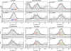 |
Fig. 6 Spectral profiles of two selected transitions for each O-bearing COM. The black curve shows the best-fit model with multiple kinematic components, and the colored dashed lines represent the contribution from each component. The blue, red, and gray bars at the bottom indicate the systemic velocities of VLA4A, VLA4B, and the circumbinary disk, respectively. The insets at the bottom of each panel show the residual from the best-fit model. |
4.3 Comparison with high-angular-resolution data
The multicomponent fitting reveals several kinematic compo- nents. Though the best-fit model has been checked (Fig. 6), we further evaluated the fitting results using high-angular-resolution data. We compared the central velocity, linewidth, and source size from the best-fit with the high-angular-resolution data. aGg’-(CH2OH)2, CH3CHO, and CH3OCHO emission was detected with ALMA at an angular resolution of ~0.″20 × 0.″11 and PA = −0.9° (~30−60 au; Diaz-Rodriguez et al. 2022).
Figure 7 shows the position-velocity (PV) diagrams from two selected transitions of aGg’-(CH2OH)2, CH3CHO, and CH3OCHO in the high resolution data, for which the PV cut is taken in the east-west direction through VLA4A and VLA4B (Fig. 1). Here we compare the best-fit VLSR, ΔV, and sizes with the PV diagrams. In the PV diagram, we plot an ellipse representing each kinematic component from the best-fit model. The width, height, and x-axis location correspond to the ΔV, source sizes, and VLSR. The y-axis offsets of ellipses were man- ually adjusted by eye. The height of the ellipse is given by (size2 + beanEW2)1/2, where beamEW is the beam size along the east–west PV cut. While the VLSR and ΔV can be directly seen in the spectral profiles (Fig. 6), the source size is obtained based on the line intensity ratios from multiple transitions with their opac- ities τ. In other words, an accurate source size suggests a good T correction with a reasonable column density as well as the temperature. As a result, each component from the lower-spatial-resolution NOEMA data is a relatively good match of the compo- nents seen in the high-spatial-resolution ALMA data, suggesting reasonable fitting of the NOEMA data at least for the three COMs, aGg’-(CH2OH)2, CH3CHO, and CH3OCHO. Again, the broad-line components in aGg’-(CH2OH)2 and CH3CHO can be ambiguous; the best-fit source sizes for the broad-line compo- nent, a/034 and 07083, are smaller than the beam of the ALMA observation. In such a case, the ALMA data do not resolve these components and only provide an upper limit to their source size. For the other components, derived source sizes are also on the same order of, or smaller than, the beam of the ALMA observations.
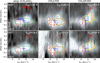 |
Fig. 7 PV diagrams of aGg’-(CH2OH)2, CH3CHO, and CH3OCHO from high-angular-resolution ALMA data (Diaz-Rodriguez et al. 2022). The dashed colored ellipses represent each kinematic component from the best-fit model (with the same colors as Fig. 6). The blue and red crosses indicate the positions and velocities of VLA4A and VLA4B, respectively. The white bar in the lower-left corner shows the beam size along the PV cut. NOEMA fits on top of the higher-resolution ALMA data match the structure, validating the NOEMA fit results. |
5 Discussion
5.1 Sizes of the O-bearing COM emission
To probe the origin of COM emission, it is crucial to estimate the size of the emitting area. The origin of COM emission can be roughly categorized into three groups: (1) hot corinos, (2) outflows, and (3) accretion shock and disk atmospheres (Belloche et al. 2020).
With the uv-domain Gaussian fitting, we find that, in our NOEMA observations at an angular resolution of 1.″2 × 0.″7 (350 × 200 au), the COM emission is a point-source like. This means it is unlikely that this emission traces the outflow cavity walls, which are usually extended.
Expected from the bolometric luminosity of SVS13A 44 L⊙, Belloche et al. (2020) estimate a radius of >40 au where the temperature is about the sublimation temperature of COMs ~ 100–150 K. Because this size is similar to the size of COM emission (see also Hsieh et al. 2019, 2023), Belloche et al. (2020) classify the COM emission in SVS 13A as a hot corino.
With the LTE model of one Gaussian component (Table 2), we derived the full width at half maximum size of each COM emission: 0.″11 (31 au for aGg’-(CH2OH)2), 0725 (74 au for CH3CHO), 0.″25 (74 au for C2H5OH), 0/22 (65 au for CH3OCHO), and 0.″31 (92 au for CH2(OH)CHO). These sizes are derived based on a number of ttansitions covering opti- cally thin to thick emission (except for CH2(OH)CHO; see Appendix B), providing an estimate of source size independent of the angular resolution of the observation (see also Sect. 4.3). These source sizes are within the sublimation radius (~30–80 au for 150–100 K) estimated by Belloche et al. (2020), but different O-bearing COMs trace different sizes (r = 16–45 au). Intu- itively, one might speculate that it is due to different sublimation temperatures of COMs or different chemical processes at work in different locations of the source; a trend of the decreasing temperature with increasing radius from ~30–8000 au is found using the derived source sizes and temperatures from molecules (Fig. 9 in Bianchi et al. 2022a). The derived Tex with source sizes (radius) are consistent with the correlation found in Bianchi et al. (2022a). With COM emission on smaller scales, we do not seen a clear trend with the limited number of data points (Fig. 8).
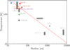 |
Fig. 8 Figure 9 from Bianchi et al. (2022a) with data points of COMs from this work. |
5.2 Complex structures
5.2.1 Kinematics
The six O-bearing COMs show different profiles (Fig. 3), sug- gesting that they come from different regions within the SVS13A system. Although the emission is not spatially resolved, their Gaussian centers at different velocities further support this scenario (Fig. 5).
Among the six O-bearing COMs, we found velocity gradi- ents from the west to the east in CH3OH, C2H5OH, CH3CHO, and CH3OCHO, while aGg’-(CH2OH)2 and CH2(OH)CHO emission do not show a velocity gradient. For aGg’-(CH2OH)2, it is consistent with the ALMA high-resolution observations by Diaz-Rodriguez et al. (2022) in which the aGg’-(CH2OH)2 emis- sion only traces the VLA4A disk. The double-peak line profiles around the VLSRof VLA4A (Fig. 3) from aGg’-CH2OH)2 and CH2(OH)CHO also imply that their emission is dominated by a rotating disk/inner envelope of VLA4A. For the other four COMs, although the velocity gradients share a similar direction from the west to the east, they have indeed different slopes. The fitted Gaussian centers may be considered as a flux-weighted centroid in a case of unresolved extended emission at the given velocity. Therefore, together with the multiple-peak spectral pro- files (Fig. 3), we speculate that the emission of these four COMs traces not only the VLA4A disk but also the VLA4B disk and/or the circumbinary disk although the VLA4A disk likely domi- nates it based on both the velocity and spatial information. Even for CH3OCHO with the most extended structure (Fig. 5), the red-shifted emission near the VLSR = 9.33 km s−1 is located around the mid-point of VLA4A and VLA4B. This is also consistent with the high-angular-resolution ALMA data (Fig. 7).
Complex organic molecule emission with different optical depths can trace different layers, as we found for  and CH3CN (Hsieh et al. 2023). In the case of protostellar envelopes, intuitively, the optically thick lines of COMs should trace the outer region while the thin transitions should trace the inner dense region. It is more complicated in Fig. 5 as each velocity step has a different optical depth. Thus, we should see the spatial distribution from low to high velocity goes across from optically thin (wing) to optically thick (middle) and back to optically thin (wing). In this case, in additional to the optically thin transitions, the blue- and redshifted line wing should point toward the cen- ter. However, this is unlikely the case; the most optically thick line of CH3OH (τ1comp. = 7.3, Table B.1), likely traces the inner region where a large velocity gradient is present (Fig. 5), while the CH3OCHO emission is associated with the outer region with τ1comp. = 0.6–1.7 (Table B.6). Alternatively, if the COM emis- sion comes from a disk, it is possible the optically thick emission lines trace the inner part of the disk where the density and tem- perature are high. However, as mentioned in Sect. 3.4, the spatial distributions are similar from different transitions with differ- ent optical depths for each COM (Fig. 5). This suggests that the discrepancy seen in the COM distribution most likely originate from chemical, rather than optical depth effects.
5.2.2 Physical conditions
Traditionally, to derive physical conditions of the gas traced by COMs, rotation diagrams and/or simple one-component Gaus- sian models are used. It is, however, frequently seen in rotation diagrams that multiple components exist with different tempera- tures (slopes) when many transitions cover wide ranges of energy levels. With this in mind, to robustly derive the physical condi- tions, we need to first identify the kinematic components with high-angular-resolution and high-spectral-resolution data with as many transitions as possible. However, this is usually very time expensive in observations.
The abundance ratios relative to CH3OH or other species, for example [X]/CH3OH, have been commonly used to study the chemical composition (e.g., Calcutt et al. 2018; Belloche et al. 2020; Jørgensen et al. 2020; Yang et al. 2021). The abun- dance ratios (![Mathematical equation: ${{\left[ {\rm{X}} \right]} \over {\left[ {{\rm{C}}{{\rm{H}}_3}{\rm{OH}}} \right]}}$](/articles/aa/full_html/2024/06/aa49417-24/aa49417-24-eq164.png) from one-velocity model, Table 2) toward SVS13A are slightly different by a factor of 0.5–2.6 to the col- umn density ratios derived by Belloche et al. (2020) except for aGg’-(CH2OH)2 with a factor of 4. In Belloche et al. (2020), the column density is derived based on the rotation diagram under an assumption of source size of 0.″3 (Table 5 in the paper). For aGg’-(CH2OH2, the difference is likely caused by a very dif- ferent rotational temperature 98 K from Belloche et al. (2020) and 240 K in this work. Here, we have included transitions with Eup ≳ 300 K as Belloche et al. (2020) use transitions with Eup < 250 K (Fig. E.29 in the paper). In the multiple-velocity component fitting, we find a possible component with a rotation temperature of 470 K that is dominant among the molecule. This explains the difference in the abundance ratio of aGg’-(CH2OH)2 (i.e.,
from one-velocity model, Table 2) toward SVS13A are slightly different by a factor of 0.5–2.6 to the col- umn density ratios derived by Belloche et al. (2020) except for aGg’-(CH2OH)2 with a factor of 4. In Belloche et al. (2020), the column density is derived based on the rotation diagram under an assumption of source size of 0.″3 (Table 5 in the paper). For aGg’-(CH2OH2, the difference is likely caused by a very dif- ferent rotational temperature 98 K from Belloche et al. (2020) and 240 K in this work. Here, we have included transitions with Eup ≳ 300 K as Belloche et al. (2020) use transitions with Eup < 250 K (Fig. E.29 in the paper). In the multiple-velocity component fitting, we find a possible component with a rotation temperature of 470 K that is dominant among the molecule. This explains the difference in the abundance ratio of aGg’-(CH2OH)2 (i.e., ![Mathematical equation: ${{\left[ {{\rm{aG}}{{\rm{g}}^\prime } - {{\left( {{\rm{C}}{{\rm{H}}_2}{\rm{OH}}} \right)}_2}} \right]} \over {\left[ {{\rm{C}}{{\rm{H}}_3}{\rm{OH}}} \right]}}$](/articles/aa/full_html/2024/06/aa49417-24/aa49417-24-eq165.png) ) derived from Belloche et al. (2020) and this work. However, toward SVS 13A, it is clear that COMs are associated with different structures. Unless the COM emission is both spectrally and spatially resolved, the dis- cussion of abundance ratios can mix together contributions of distinct structures, providing no quantitative physical constraints needed for chemical models.
) derived from Belloche et al. (2020) and this work. However, toward SVS 13A, it is clear that COMs are associated with different structures. Unless the COM emission is both spectrally and spatially resolved, the dis- cussion of abundance ratios can mix together contributions of distinct structures, providing no quantitative physical constraints needed for chemical models.
Our NOEMA observations cover a number of transitions for modeling at a high-spectral-resolution (Tables B.1–B.6). Thus, multiple kinematic components can be disentangled and their physical conditions can be derived (Table 2; see also Hsieh et al. 2023 for CH3CN). Figure 9 shows the tempera- ture of these kinematic components as a function of velocity (Table 2). For the one-component model, it unveils that the different O-bearing COMs are tracing different regions with dif- ferent temperatures and source sizes. The multicomponent fitting further unveils several components with temperatures ranging from a few tens to a few hundred kelvin. It is likely that the one-component model usually gives a temperature between those derived from multiple-component model. However, the total amount of molecules (i.e., Ntot×area in Table 2) is always higher in multiple-component fitting; the sum of the Ntot×area from the multiple-component fitting is larger than that of single compo- nent fitting by a factor of 1.1–1.5 (see ![Mathematical equation: ${{[{\rm{X}}]} \over {\left[ {{\rm{C}}{{\rm{H}}_3}{\rm{OH}}} \right]}}$](/articles/aa/full_html/2024/06/aa49417-24/aa49417-24-eq166.png) in Table 2. That is because the multiple-component fitting process may unveil hidden components from the complex line profile (Hsieh et al. 2023). Also, these components are assumed to be spatially sepa- rated so that the integrated τ from the multi-velocity model can be larger than that of the single component.
in Table 2. That is because the multiple-component fitting process may unveil hidden components from the complex line profile (Hsieh et al. 2023). Also, these components are assumed to be spatially sepa- rated so that the integrated τ from the multi-velocity model can be larger than that of the single component.
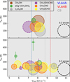 |
Fig. 9 Excitation temperature as a function of central velocity for the six O-bearing COMs. The top panel shows the results from sin- gle component fitting, and the bottom panel shows the results from the multicomponent fit. The size of the circle represents the source size; the CH2(OH)CHO circle has a dashed outline since the source size of CH2(OH)CHO can be degenerate with column density due to a lack of optically thick transition. The dashed circle at the bottom-right corner indicates a size of 0.3 arcsec. |
5.3 Origin of COM emission in SVS13A
Thanks to the capabilities of the N EMA PolyFiX correlator, we have identified multiple velocity components toward SVS13A, and better quantified the kinematics and physical conditions using six O-bearing COMs. It is clear that the COM emis- sion traces different kinematic components toward SVS13A with different physical conditions (temperature, column density and size). This suggests that the COM emission in SVS13A origi- nates from a complex structure, which may not be explained by a unique scenario.
It is interesting to compare with the well-studied hot corino protobinary system IRAS 16293-2422A (hereafter IRAS 16293A) at an earlier evolutionary stage than SVS13A (Pineda et al. 2012; Jørgensen et al. 2016; Ceccarelli et al. 2022). With high-angular-resolution ALMA observations, Maureira et al. (2020) found complex structures toward IRAS 16293A traced by HNCO, NH2CHO, and t–HCOOH. Maureira et al. (2022) find that these complex structures are asso- ciated with hot dust and gas spots (see also Oya & Yamamoto 2020). The kinematic, spatial distribution, and temperature were in agreement with predictions from shocks. Shocks are expected, for example, due to the landing of inalling streamers in the disk high-density material. Indeed, an infalling streamer induc- ing local shocks has been found by Garufi et al. (2022) via SO toward a more evolved young stellar object HL Tau (see also van Gelder et al. 2021); an infalling streamer toward IRAS 16293A is also suggested by Murillo et al. (2022). This hints at a sce- nario where the physical and chemical properties of an inner region (≲300 au) is affected by large-scale (approximately a few thousand au) infalling streamers (see Pineda et al. 2023 and references therein).
Toward SVS13A, Hsieh et al. (2023) suggest that the contin- uum spiral structure connected to VLA4A is associated with a streamer from larger scales, which is possibly infalling. Bianchi et al. (2022b) speculate that streamer-induced shocks sputter icy COMs from dust grains given the asymmetric structure of COM emission toward SVS13A from high-angular-resolution data. In this work, we find that the COM emission traces com- plex structures, so it is unlikely only due to heating from the central protostellar source. Thus, we consider that shocks from materials infalling onto and impacting circumstellar or circumbinary disks play an important role in feeding COMs from dust grains, leading to the complex structure in COM emission. Other possibilities are shocks produced by the self-gravity or tidal forces within the disks themselves. To understand this requires high-angular-resolution observations, coupled with high spectral resolution and sensitivity.
6 Conclusion
We present NOEMA observations toward SVS13A of six selected O-bearing COMs. The spectral profiles reveal multiple kinematic velocity components that trace different physical enti- ties as well as their distinctive spatial distributions, suggesting that the emission from each COM species can come from dif- ferent regions. We derive their physical conditions, finding that these COMs trace a complex structure in the protobinary system SVS13A. Our main conclusions are summarized as follows:
Toward the protobinary system SVS13A, we find that for a given COM species, the spatial distributions of different transitions show similar structures based on the uv-space Gaussian fitting at different velocities. However, different COMs do not trace the same kinematic components. This necessitates a caveat when discussing the abundance ratios and chemical properties of COMs without kinematically resolving the systems. The measurement of relative COM abundances requires high-spectral-resolution (as well as high-angular-resolution) observations.
By covering numerous transitions with high spectral resolu- tion, we decomposed the emission of each COM into several kinematic components. We suggest that the traditional rota- tional diagram or one-component fitting can underestimate the total amount of molecules. We find that each COM can contain multiple velocity components within tens of astronomical units of the hot corino, which trace different physical conditions.
We find that the COM emission from SVS13A is associ- ated with an inhomogeneous complex structure. The small source sizes show that the emission likely does not arise from outflow cavity walls. It is unlikely that this complex structure is caused only by heating from the central proto- star. We conclude that the COM emission most likely comes from shocked gas at disk scales. The shocked gas may be induced by the large-scale streamer (Hsieh et al. 2023), which may be infalling directly onto the disk and producing inhomogeneous shocked regions.
Our results suggest that different COMs can trace very differ- ent kinematic components in a system. This means we have to be careful when comparing abundances before resolving the system. The emission of an individual COM can be associated with multiple components. This suggests that COM emission is influenced by localized shock activities instead of only the protostellar heating.
Acknowledgements
We are grateful for the anonymous referee for the thor- ough and insightful comments that helped to improve this paper significantly. T.-H.H., J.E.P., P.C., M.T.V, C.G., and M.J.M. acknowledge the support by the Max Planck Society. The authors thank Eleonora Bianchi Valerio Lat- tanzi, Silvia Spezzano, and Christian Endres for the chemical modeling and CDMS. D.S.-C. is supported by an NSF Astronomy and Astrophysics Post- doctoral Fellowship under award AST-2102405. I.J-.S acknowledges funding from grants No. PID2019-105552RB-C41 and PID2022-136814NB-I00 funded by MICIU/AEI/10.13039/501100011033 and by “ERDF/EU”. This work is based on observations carried out under project number L19MB with the IRAM NOEMA Interferometer. IRAM is supported by INSU/CNRS (France), MPG (Germany) and IGN (Spain). This paper makes use of the following ALMA data: ADS/JAO.ALMA#2013.1.00031.S and 2016.1.01305. ALMA is a partner- ship of ESO (representing its member states), NSF (USA) and NINS (Japan), together with NRC (Canada), MOST and ASIAA (Taiwan), and KASI (Repub- lic of Korea), in cooperation with the Republic of Chile. The Joint ALMA Observatory is operated by ESO, AUI/NRAO and NAOJ. S.M. is supported by a Royal Society University Research Fellowship (URF-R1-221669). D.S. and Th.H. acknowledge support from the European Research Council under the Hori- zon 2020 Framework Program via the ERC Advanced Grant Origins 83 24 28. A.F. thanks the Spanish MICIN for funding support from PID2019-106235GB-100 and the European Research Council (ERC) for funding under the Advanced Grant project SUL4LIFE, grant agreement No101096293.
Software: Numpy (Van Der Walt et al. 2011), Scipy (Virtanen et al. 2020), APLpy (Robitaille & Bressert 2012), Matplotlib (Hunter 2007), Astropy (Astropy Collaboration 2013), CASA (McMullin et al. 2007).
Appendix A Line stacking
To unveil the complexity of the line profiles, we stacked spectra from manually selected transitions using SciPy and NumPy; these transitions were selected to have similar line profiles and to not be contaminated by other lines. Figure A.1 shows the individual line profiles in comparison to the stacked line profiles presented in Fig. 3. These transitions are selected as they share similar normalized spectrum profiles; we compared the averaged profiles with the candidate transition to see if they look similar. If yes, the transition was added for stacking. In the off-peak velocities, the continuum-subtracted fluxes sometimes do not reach zero since they can still be affected by contamination from other molecular line transitions.
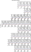 |
Fig. A.1 All spectral profiles used for the line stacking. Each column shows all the transitions of a particular species used in the line stacking, as gray-filled histograms. The black histograms represent the resulting stacked spectrum of each molecule, for comparison. |
Appendix B Line fitting
Figures B.1 to B.6 show the best-fit profiles of the one-component fitting for all transitions in use (see Sect. 4.1). Figure B.7 shows the relative intensity as a function of the upper energy level for those transitions involved in the fitting; more importantly, the colors represent the optical depths from the single-component fitting. The transitions used are listed in Tables B.1 to B.6; they are summarized in the CDMS, with individual molecule originally measured by: CH3OH (Xu et al. 2008), aGg’-(CH2OH)2 (Christen & Müller 2003), C2H5OH (Pearson et al. 2008; Müller et al. 2016), CH2(OH)CHO (Butler et al. 2001), CH3CHO (Kleiner et al. 1996), CH3OCHO (Ilyushin et al. 2009), and CH3OCH3 (Endres et al. 2009). Optically thick lines are required in order to derive the source size (see Sect. 4.1). On the other hand, a broad range of Eup will constrain the physical conditions and perhaps identify different temperature components. Also, a large number of transitions in use is crucial, especially for multicomponent fitting.
For each COM, we started by fitting one component and added an extra component with each iteration of the fit. For each iteration, χ2 and ΔAIC were calculated to help evaluate if adding one more component would improve the fit (Table 3). We stopped adding additional components when the χ2 did not significantly improve relative to the previous iteration and/or the fitting found an unreasonable component. Take C2H5OH as an example. We stopped adding a new component at the two-component model because the third component contributes emission at about the noise level with an extreme high optical depth (9 × 1022 cm−2). Whether this component is real or not is difficult to judge with the current dataset and severe line contamination in this source. Therefore, we adopted the two-component model for C2H5OH. After the numbers of components were determined, we conducted MCMC fitting using emcee as well as one-component fitting.
Transitions for the fitting: CH3OH.
Transitions for the fitting: aGg’-(CH2OH)2.
Transitions for the fitting: C2H5OH.
Transitions for the fitting: CH2(OH)CHO.
Transitions for the fitting: CH3CHO.
Transitions for the fitting: CH3OCHO.
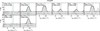 |
Fig. B.1 Modeled CH3OH line profiles overlaid on the observed spectra. The three vertical dashed lines show the central velocities of VLA4A (blue), VLA4B (red), and the circumbinary system (gray). The subpanel at the bottom shows the residual from the best fit. The green bars mark the velocities of VLA4A (7.36 km s−1) for all transitions used in the model of CH3OH. |
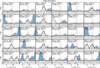 |
Fig. B.2 Same as Fig. B.1 but for aGg’-(CH2OH)2. The hatch indicates the regions that are masked for the fitting. |
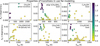 |
Fig. B.7 Properties of the transitions in use for the modeling. The color of the data points indicates the optical depth for each transition from the single velocity component model. The label “Good” indicates that the energy levels are well sampled by the transitions, allowing us to derive the temperature, and that they cover optically thick emission, allowing us to derive the source size. |
Appendix C CH3OCH3
CH3OCH3 is detected in the narrowband high-resolution data in only a few transitions without contamination from other lines (Fig. C.1). The only detection with high S/N ratio, 72,5 − 61,6, is blended by other transitions so that we cannot analyze the kinematics like in Figs. 3 and 5. One-component LTE fitting is conducted, yielding a source with Tex = 173 K, V1sr = 9.1 km s−1, and FWHM= 2.71 km s−1. The source size and column density is not well constrained given all optically thin (τ < 0.2) line emission. CH3OCH3 and CH3OCHO are considered to be chemically linked (for example Coletta et al. 2020). The one-component models do not provide the same temperature and V1sr, but this could simply be due to the very limited number of transitions available in the case of CH3OCH3.
References
- Alves, F. O., Cleeves, L. I., Girart, J. M., et al. 2020, ApJ, 904, L6 [NASA ADS] [CrossRef] [Google Scholar]
- Anglada, G., Rodríguez, L. F., Osorio, M., et al. 2004, ApJ, 605, L137 [Google Scholar]
- Arce, H. G., Santiago-García, J., Jørgensen, J. K., et al. 2008, ApJ, 681, L21 [NASA ADS] [CrossRef] [Google Scholar]
- Astropy Collaboration (Robitaille, T. P., et al.) 2013, A&A, 558, A33 [NASA ADS] [CrossRef] [EDP Sciences] [Google Scholar]
- Bacmann, A., Taquet, V., Faure, A., et al. 2012, A&A, 541, L12 [NASA ADS] [CrossRef] [EDP Sciences] [Google Scholar]
- Belloche, A., Maury, A. J., Maret, S., et al. 2020, A&A, 635, A198 [NASA ADS] [CrossRef] [EDP Sciences] [Google Scholar]
- Bianchi, E., Codella, C., Ceccarelli, C., et al. 2017, MNRAS, 467, 3011 [NASA ADS] [CrossRef] [Google Scholar]
- Bianchi, E., Codella, C., Ceccarelli, C., et al. 2019, MNRAS, 483, 1850 [Google Scholar]
- Bianchi, E., Ceccarelli, C., Codella, C., et al. 2022a, A&A, 662, A103 [NASA ADS] [CrossRef] [EDP Sciences] [Google Scholar]
- Bianchi, E., López-Sepulcre, A., Ceccarelli, C., et al. 2022b, ApJ, 928, L3 [NASA ADS] [CrossRef] [Google Scholar]
- Blake, G. A., Sutton, E. C., Masson, C. R., et al. 1987, ApJ, 315, 621 [NASA ADS] [CrossRef] [Google Scholar]
- Bottinelli, S., Ceccarelli, C., Lefloch, B., et al. 2004, ApJ, 615, 354 [Google Scholar]
- Bottinelli, S., Ceccarelli, C., Williams, J. P., et al. 2007, A&A, 463, 601 [NASA ADS] [CrossRef] [EDP Sciences] [Google Scholar]
- Bouvier, M., López-Sepulcre, A., Ceccarelli, C., et al. 2021, A&A, 653, A117 [CrossRef] [EDP Sciences] [Google Scholar]
- Butler, R. A. H., De Lucia, F. C., Petkie, D. T., et al. 2001, ApJS, 134, 319 [CrossRef] [Google Scholar]
- Cabedo, V., Maury, A., Girart, J. M., et al. 2021, A&A, 653, A166 [NASA ADS] [CrossRef] [EDP Sciences] [Google Scholar]
- Calcutt, H., Jørgensen, J. K., Müller, H. S. P., et al. 2018, A&A, 616, A90 [NASA ADS] [CrossRef] [EDP Sciences] [Google Scholar]
- Caselli, P., & Ceccarelli, C. 2012, A&A Rev., 20, 56 [NASA ADS] [CrossRef] [Google Scholar]
- Cazaux, S., Tielens, A. G. G. M., Ceccarelli, C., et al. 2003, ApJ, 593, L51 [CrossRef] [Google Scholar]
- Ceccarelli, C., Caselli, P., Fontani, F., et al. 2017, ApJ, 850, 176 [NASA ADS] [CrossRef] [Google Scholar]
- Ceccarelli, C., Codella, C., Balucani, N., et al. 2022, arXiv e-prints [arXiv:2206.13270] [Google Scholar]
- Choudhury, S., Pineda, J. E., Caselli, P., et al. 2020, A&A, 640, L6 [EDP Sciences] [Google Scholar]
- Christen, D., & Müller, H. S. P. 2003, Phys. Chem. Chem. Phys., 5, 3600 [NASA ADS] [CrossRef] [Google Scholar]
- Christen, D., Coudert, L. H., Larsson, J. A., et al. 2001, J. Mol. Spectrosc., 205, 185 [NASA ADS] [CrossRef] [Google Scholar]
- Codella, C., Bianchi, E., Tabone, B., et al. 2018, A&A, 617, A10 [NASA ADS] [CrossRef] [EDP Sciences] [Google Scholar]
- Codella, C., Bianchi, E., Podio, L., et al. 2021, A&A, 654, A52 [NASA ADS] [CrossRef] [EDP Sciences] [Google Scholar]
- Coletta, A., Fontani, F., Rivilla, V. M., et al. 2020, A&A, 641, A54 [NASA ADS] [CrossRef] [EDP Sciences] [Google Scholar]
- Csengeri, T., Bontemps, S., Wyrowski, F., et al. 2018, A&A, 617, A89 [NASA ADS] [CrossRef] [EDP Sciences] [Google Scholar]
- Csengeri, T., Belloche, A., Bontemps, S., et al. 2019, A&A, 632, A57 [NASA ADS] [CrossRef] [EDP Sciences] [Google Scholar]
- Diaz-Rodriguez, A. K., Anglada, G., Blázquez-Calero, G., et al. 2022, ApJ, 930, 91 [NASA ADS] [CrossRef] [Google Scholar]
- Drozdovskaya, M. N., Walsh, C., Visser, R., et al. 2015, MNRAS, 451, 3836 [NASA ADS] [CrossRef] [Google Scholar]
- Endres, C. P., Drouin, B. J., Pearson, J. C., et al. 2009, A&A, 504, 635 [NASA ADS] [CrossRef] [EDP Sciences] [Google Scholar]
- Endres, C. P., Schlemmer, S., Schilke, P., et al. 2016, J. Mol. Spectrosc., 327, 95 [NASA ADS] [CrossRef] [Google Scholar]
- Foreman-Mackey, D., Hogg, D. W., Lang, D., et al. 2013, PASP, 125, 306 [NASA ADS] [CrossRef] [Google Scholar]
- Garufi, A., Dominik, C., Ginski, C., et al. 2022, A&A, 658, A137 [NASA ADS] [CrossRef] [EDP Sciences] [Google Scholar]
- Gieser, C., Beuther, H., Semenov, D., et al. 2023, A&A, 674, A160 [NASA ADS] [CrossRef] [EDP Sciences] [Google Scholar]
- Ginski, C., Facchini, S., Huang, J., et al. 2021, ApJ, 908, L25 [NASA ADS] [CrossRef] [Google Scholar]
- Goodman, J., & Weare, J. 2010, Commun. Appl. Math. Comput. Sci., 5, 65 [Google Scholar]
- Harsono, D., Visser, R., Bruderer, S., et al. 2013, A&A, 555, A45 [NASA ADS] [CrossRef] [EDP Sciences] [Google Scholar]
- Herbst, E., & van Dishoeck, E. F. 2009, ARA&A, 47, 427 [NASA ADS] [CrossRef] [Google Scholar]
- Hogg, D. W., & Foreman-Mackey, D. 2018, ApJS, 236, 11 [NASA ADS] [CrossRef] [Google Scholar]
- Hsieh, T.-H., Murillo, N. M., Belloche, A., et al. 2019, ApJ, 884, 149 [Google Scholar]
- Hsieh, T.-H., Segura-Cox, D. M., Pineda, J. E., et al. 2023, A&A, 669, A137 [NASA ADS] [CrossRef] [EDP Sciences] [Google Scholar]
- Hunter, J. D. 2007, Comput. Sci. Eng., 9, 90 [NASA ADS] [CrossRef] [Google Scholar]
- Ilyushin, V., Kryvda, A., & Alekseev, E. 2009, J. Mol. Spectrosc., 255, 32 [NASA ADS] [CrossRef] [Google Scholar]
- Jørgensen, J. K., Hogerheijde, M. R., Blake, G. A., et al. 2004, A&A, 415, 1021 [NASA ADS] [CrossRef] [EDP Sciences] [Google Scholar]
- Jørgensen, J. K., van der Wiel, M. H. D., Coutens, A., et al. 2016, A&A, 595, A117 [Google Scholar]
- Jørgensen, J. K., Müller, H. S. P., Calcutt, H., et al. 2018, A&A, 620, A170 [Google Scholar]
- Jørgensen, J. K., Belloche, A., & Garrod, R. T. 2020, ARA&A, 58, 727 [Google Scholar]
- Kleiner, I., Lovas, F. J., & Godefroid, M. 1996, J. Phys. Chem. Ref. Data, 25, 1113 [CrossRef] [Google Scholar]
- Lefèvre, C., Cabrit, S., Maury, A. J., et al. 2017, A&A, 604, L1 [CrossRef] [EDP Sciences] [Google Scholar]
- Lefloch, B., Bachiller, R., Ceccarelli, C., et al. 2018, MNRAS, 477, 4792 [Google Scholar]
- Maureira, M. J., Pineda, J. E., Segura-Cox, D. M., et al. 2020, ApJ, 897, 59 [NASA ADS] [CrossRef] [Google Scholar]
- Maureira, M. J., Gong, M., Pineda, J. E., et al. 2022, ApJ, 941, L23 [NASA ADS] [CrossRef] [Google Scholar]
- McMullin, J. P., Waters, B., Schiebel, D., et al. 2007, Astronomical Data Analysis Software and Systems XVI, 376, 127 [NASA ADS] [Google Scholar]
- Möller, T., Endres, C., & Schilke, P. 2017, A&A, 598, A7 [NASA ADS] [CrossRef] [EDP Sciences] [Google Scholar]
- Müller, H. S. P., Schlöder, F., Stutzki, J., et al. 2005, J. Mol. Struc., 742, 215 [CrossRef] [Google Scholar]
- Müller, H. S. P., Belloche, A., Xu, L.-H., et al. 2016, A&A, 587, A92 [NASA ADS] [CrossRef] [EDP Sciences] [Google Scholar]
- Murillo, N. M., van Dishoeck, E. F., Hacar, A., et al. 2022, A&A, 658, A53 [NASA ADS] [CrossRef] [EDP Sciences] [Google Scholar]
- Ortiz-León, G. N., Loinard, L., Dzib, S. A., et al. 2018, ApJ, 869, L33 [Google Scholar]
- Oya, Y., & Yamamoto, S. 2020, ApJ, 904, 185 [NASA ADS] [CrossRef] [Google Scholar]
- Oya, Y., Sakai, N., López-Sepulcre, A., et al. 2016, ApJ, 824, 88 [Google Scholar]
- Palau, A., Walsh, C., Sánchez-Monge, Á., et al. 2017, MNRAS, 467, 2723 [NASA ADS] [Google Scholar]
- Pearson, J. C., Brauer, C. S., & Drouin, B. J. 2008, J. Mol. Spectrosc., 251, 394 [NASA ADS] [CrossRef] [Google Scholar]
- Pineda, J. E., Maury, A. J., Fuller, G. A., et al. 2012, A&A, 544, L7 [NASA ADS] [CrossRef] [EDP Sciences] [Google Scholar]
- Pineda, J. E., Segura-Cox, D., Caselli, P., et al. 2020, Nat. Astron., 4, 1158 [NASA ADS] [CrossRef] [Google Scholar]
- Pineda, J. E., Arzoumanian, D., André, P., et al. 2023, ASP Conf. Ser., 534, 233 [NASA ADS] [Google Scholar]
- Robitaille, T., & Bressert, E. 2012, Astrophysics Source Code Library [record ascl:1208.017] [Google Scholar]
- Sargent, A. I., & Beckwith, S. 1987, ApJ, 323, 294 [NASA ADS] [CrossRef] [Google Scholar]
- Segura-Cox, D. M., Looney, L. W., Tobin, J. J., et al. 2018, ApJ, 866, 161 [Google Scholar]
- Spezzano, S., Bizzocchi, L., Caselli, P., et al. 2016, A&A, 592, L11 [NASA ADS] [CrossRef] [EDP Sciences] [Google Scholar]
- Sugimura, M., Yamaguchi, T., Sakai, T., et al. 2011, PASJ, 63, 459 [NASA ADS] [Google Scholar]
- Tafalla, M., Santiago-García, J., Myers, P. C., et al. 2006, A&A, 455, 577 [NASA ADS] [CrossRef] [EDP Sciences] [Google Scholar]
- Thieme, T. J., Lai, S.-P., Lin, S.-J., et al. 2022, ApJ, 925, 32 [NASA ADS] [CrossRef] [Google Scholar]
- Tobin, J. J., Looney, L. W., Li, Z.-Y., et al. 2016, ApJ, 818, 73 [CrossRef] [Google Scholar]
- Tobin, J. J., Looney, L. W., Li, Z.-Y., et al. 2018, ApJ, 867, 43 [CrossRef] [Google Scholar]
- Tychoniec, Ł., Manara, C. F., Rosotti, G. P., et al. 2020, A&A, 640, A19 [NASA ADS] [CrossRef] [EDP Sciences] [Google Scholar]
- Valdivia-Mena, M. T., Pineda, J. E., Segura-Cox, D. M., et al. 2022, A&A, 667, A12 (Paper I) [NASA ADS] [CrossRef] [EDP Sciences] [Google Scholar]
- Van Der Walt, S., Colbert, S. C., & Varoquaux, G. 2011, Comput. Sci. Eng., 13, 22 [Google Scholar]
- van Dishoeck, E. F., Blake, G. A., Jansen, D. J., et al. 1995, ApJ, 447, 760 [NASA ADS] [CrossRef] [Google Scholar]
- van Dishoeck, E. F. 2014, Faraday Discuss., 168, 9 [NASA ADS] [CrossRef] [Google Scholar]
- van Gelder, M. L., Tabone, B., van Dishoeck, E. F., et al. 2021, A&A, 653, A159 [CrossRef] [EDP Sciences] [Google Scholar]
- Vastel, C., Alves, F., Ceccarelli, C., et al. 2022, A&A, 664, A171 [NASA ADS] [CrossRef] [EDP Sciences] [Google Scholar]
- Virtanen, P., Gommers, R., Oliphant, T. E., et al. 2020, Nat. Meth., 17, 261 [Google Scholar]
- Xu, L.-H., Fisher, J., Lees, R. M., et al. 2008, J. Mol. Spectrosc., 251, 305 [NASA ADS] [CrossRef] [Google Scholar]
- Yang, Y.-L., Sakai, N., Zhang, Y., et al. 2021, ApJ, 910, 20 [Google Scholar]
All Tables
All Figures
|
Fig. 1 Integrated intensity maps of a selected transition for each O-bearing COM. The top-right panel in each figure shows the spectra toward the center, and the filled regions indicate the integration range for the zero-order moment maps, which is 3.5–10.7 km s−1 (except for CH3OH, for which it is 3.5–12.0 km s−1), for the zero-order moment maps. The blue contours in the top-left panel represent the ALMA 1.3 mm continuum emission (Tobin et al. 2018) with levels of [3, 5, 7, 10, 30, 70]σ. The horizontal gray line in the top-left panel shows the PV cut used in Fig. 7. The blue pixel in the top-right panel is the pixel used to extract the spectra in this work. |
| In the text | |
|
Fig. 2 Low-spectral-resolution spectrum toward the continuum peak of SVS13A from the PRODIGE NOEMA large program. The panels, from top to bottom, represent the spectra from the receiver bands as shown in the sketch in the middle. The horizontal orange bars represent locations of the high-spectral-resolution windows. |
| In the text | |
|
Fig. 3 Comparison of stacked line profiles of the six O-bearing COMs. The stacking was done using spectra normalized to their peak fluxes and weighting with the reciprocal of noise squared (Appendix A). The vertical dashed lines indicate the central velocities of the disks of VLA4A (blue), 4B (red), and the circumbinary disk (gray) from Diaz-Rodriguez et al. (2022). |
| In the text | |
|
Fig. 4 Gaussian linewidth versus central velocity of the selected transitions from the six O-bearing COMs. The vertical dashed lines rep- resent the central velocities of the disks of VLA4A (blue), 4B (red), and the circumbinary disk (gray). The transitions in use are listed in Tables B.1–B.6. |
| In the text | |
|
Fig. 5 Central positions of selected COM transitions at different velocities. The top two panels show the integrated intensity map (left) and central positions (right) from CH3CN (Hsieh et al. 2023) as a reference for the O-bearing COMs. The contours show the 1.3 mm continuum emission from Tobin et al. (2018). Different line transitions are marked with different symbols (Tables B.1-B.6). The scale bar is 0.″1 for the bottom six panels. The beam sizes for these COM emissions depend on the line frequency but are the same as that of CH3CN (1.″2 × 077) within 10%. |
| In the text | |
|
Fig. 6 Spectral profiles of two selected transitions for each O-bearing COM. The black curve shows the best-fit model with multiple kinematic components, and the colored dashed lines represent the contribution from each component. The blue, red, and gray bars at the bottom indicate the systemic velocities of VLA4A, VLA4B, and the circumbinary disk, respectively. The insets at the bottom of each panel show the residual from the best-fit model. |
| In the text | |
|
Fig. 7 PV diagrams of aGg’-(CH2OH)2, CH3CHO, and CH3OCHO from high-angular-resolution ALMA data (Diaz-Rodriguez et al. 2022). The dashed colored ellipses represent each kinematic component from the best-fit model (with the same colors as Fig. 6). The blue and red crosses indicate the positions and velocities of VLA4A and VLA4B, respectively. The white bar in the lower-left corner shows the beam size along the PV cut. NOEMA fits on top of the higher-resolution ALMA data match the structure, validating the NOEMA fit results. |
| In the text | |
|
Fig. 8 Figure 9 from Bianchi et al. (2022a) with data points of COMs from this work. |
| In the text | |
|
Fig. 9 Excitation temperature as a function of central velocity for the six O-bearing COMs. The top panel shows the results from sin- gle component fitting, and the bottom panel shows the results from the multicomponent fit. The size of the circle represents the source size; the CH2(OH)CHO circle has a dashed outline since the source size of CH2(OH)CHO can be degenerate with column density due to a lack of optically thick transition. The dashed circle at the bottom-right corner indicates a size of 0.3 arcsec. |
| In the text | |
|
Fig. A.1 All spectral profiles used for the line stacking. Each column shows all the transitions of a particular species used in the line stacking, as gray-filled histograms. The black histograms represent the resulting stacked spectrum of each molecule, for comparison. |
| In the text | |
|
Fig. B.1 Modeled CH3OH line profiles overlaid on the observed spectra. The three vertical dashed lines show the central velocities of VLA4A (blue), VLA4B (red), and the circumbinary system (gray). The subpanel at the bottom shows the residual from the best fit. The green bars mark the velocities of VLA4A (7.36 km s−1) for all transitions used in the model of CH3OH. |
| In the text | |
|
Fig. B.2 Same as Fig. B.1 but for aGg’-(CH2OH)2. The hatch indicates the regions that are masked for the fitting. |
| In the text | |
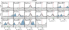 |
Fig. B.3 Same as Fig. B.2 but for C2H5OH. |
| In the text | |
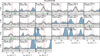 |
Fig. B.4 Same as Fig. B.2 but for CH2(OH)CHO. |
| In the text | |
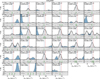 |
Fig. B.5 Same as Fig. B.2 but for CH3CHO. |
| In the text | |
 |
Fig. B.6 Same as Fig. B.2 but for CH3OCHO. |
| In the text | |
|
Fig. B.7 Properties of the transitions in use for the modeling. The color of the data points indicates the optical depth for each transition from the single velocity component model. The label “Good” indicates that the energy levels are well sampled by the transitions, allowing us to derive the temperature, and that they cover optically thick emission, allowing us to derive the source size. |
| In the text | |
 |
Fig. C.1 Same as Fig. B.2 but for CH3OCH3. |
| In the text | |
Current usage metrics show cumulative count of Article Views (full-text article views including HTML views, PDF and ePub downloads, according to the available data) and Abstracts Views on Vision4Press platform.
Data correspond to usage on the plateform after 2015. The current usage metrics is available 48-96 hours after online publication and is updated daily on week days.
Initial download of the metrics may take a while.