| Issue |
A&A
Volume 696, April 2025
|
|
|---|---|---|
| Article Number | A228 | |
| Number of page(s) | 21 | |
| Section | Extragalactic astronomy | |
| DOI | https://doi.org/10.1051/0004-6361/202452983 | |
| Published online | 25 April 2025 | |
Clump formation in ram-pressure stripped galaxies: Evidence from mass function
1
Dipartimento di Fisica e Astronomia “Augusto Righi”, Università di Bologna, via Piero Gobetti 93/2, I-40129 Bologna, Italy
2
Minnesota Institute for Astrophysics, School of Physics and Astronomy, University of Minnesota, 316 Church Street SE, Minneapolis, MN 55455, USA
3
INAF-Osservatorio Astronomico di Padova, Vicolo Osservatorio 5, 35122 Padova, Italy
4
Dipartimento di Fisica e Astronomia, Università di Padova, Vicolo Osservatorio 3, 35122 Padova, Italy
5
INAF – Osservatorio Astronomico di Brera, via Brera, 28, 20121 Milano, Italy
⋆ Corresponding author: eric.giunchi2@unibo.it
Received:
13
November
2024
Accepted:
17
February
2025
Context. The mass function (MF) of young stellar clumps (age ≲ 200 Myr) is an indicator of the mechanism driving the collapse of the interstellar medium (ISM) into the giant molecular clouds. Typically, the MF of clumps in main-sequence galaxies is described by a power law (dN/dM* ∝ M*−α) with slope α = 2, hinting that the collapse is driven by turbulence.
Aims. To understand whether the local environment affects star formation, we modelled the clump MF of six cluster galaxies, from the GASP survey, undergoing strong ram-pressure stripping (RPS). This phenomenon, exerted by the hot and high-pressure intracluster medium (ICM), has produced long tails of stripped ISM, where clumps form far away from the galactic disk and are surrounded by the ICM itself.
Methods. Clumps were selected from HST-UVIS/WFC3 images, covering from near-UV to red-optical bands and including Hα emission-line maps. The catalogue comprises 398 Hα clumps (188 in tails, 210 in the disk outskirts known as the extraplanar region) and 1270 UV clumps (593 in tails, 677 extraplanar). Using mock images, we quantified the mass completeness and bias of our sample. Taking these two effects into account, we adopted a Bayesian approach to fit the clump mass catalogue to a suitable MF.
Results. The resulting MFs are steeper than the expected value of 2. In the tails the Hα clumps have slope α = 2.31 ± 0.12, while the UV slope is larger (2.60 ± 0.09), in agreement with ageing effects. Similar results are found in the extraplanar region, with Hα slope α = 2.45−0.16+0.20 and UV slope α = 2.63−0.18+0.20, even though in this case they are consistent within the uncertainties.
Conclusions. We suggest that the steepening results from the higher-than-usual turbulent environment, arising from the interaction between the ISM and the ICM. As shown by recent works, this process can favour the fragmentation of the largest ISM clouds, inhibiting the formation of very massive clumps.
Key words: galaxies: clusters: general / galaxies: evolution / galaxies: peculiar / galaxies: star formation / galaxies: structure
© The Authors 2025
 Open Access article, published by EDP Sciences, under the terms of the Creative Commons Attribution License (https://creativecommons.org/licenses/by/4.0), which permits unrestricted use, distribution, and reproduction in any medium, provided the original work is properly cited.
This article is published in open access under the Subscribe to Open model. Subscribe to A&A to support open access publication.
1. Introduction
It is currently widely accepted that the formation of new stars in galaxies occurs in the density peaks of the cold molecular gas, in the cores of the giant molecular clouds (Lada & Lada 2003; Bressert et al. 2010). These dense and cold regions represent the final stage of a complex process that involves turbulence, gas cooling, and the growth of non-linear perturbation, which drives the condensation of atomic gas (mainly neutral hydrogen, H I) from galactic to sub-kiloparsec scales down to the parsec/sub-parsec dense cores of cold molecular gas (Kennicutt & Evans 2012). In this scenario, ≳10 pc scaled star-forming clusters and compact groups of stellar clusters (called clumps), with masses ≳104 M⊙ (Portegies Zwart et al. 2010), represent the connecting piece between the galactic-scale and core-scale regimes. These stellar clusters are the smallest structures in galaxies containing enough stars to fully sample the stellar initial mass function (IMF). Therefore, they represent suitable sites to study in a statistical way the star formation mechanism as a function of the clump environment, such as the global properties of the host galaxy, whether the host galaxy itself is in the field or in a cluster and the local conditions of the medium in which the stellar clumps and the molecular gas clouds are embedded.
Models describing the fragmentation of star-forming regions as a scale-free turbulence-driven process predict that the mass function MF ≡ dN/dM* of these regions (i.e. the number of objects per mass bin) is a power law in the form
with α = 2 (Elmegreen 2002, 2006). Similar results are found in simulations of neutral atomic and molecular medium clump formation (Renaud et al. 2024). Other theoretical works find slightly flatter distributions (α = 1.7 − 1.8) (Hennebelle & Audit 2007; Audit & Hennebelle 2010; Fensch et al. 2023), especially when increasing the gas fraction (Renaud et al. 2024). As time proceeds after the clump formation, the slope of the clump mass function is thought to change, as a consequence of many processes, including the clump dynamical evolution, relaxation, and the interactions within the surrounding environment. However, whether the net effect is the steepening or the flattening the mass function (Gieles 2009; Fujii & Portegies Zwart 2015) is still debated since many observational effects make the comparison with models difficult.
The launch of the Hubble Space Telescope (HST) has provided the possibility to perform unprecedented high-resolution observational surveys of low-redshift galaxies (LEGUS, Calzetti et al. 2015; DYNAMO, Fisher et al. 2017; LARS, Messa et al. 2019; PHANGS-HST, Lee et al. 2022), which have brought great improvements to our knowledge about star-forming clumps. These surveys covered galaxies in very different regimes and environments, from normal spirals (e.g. in LEGUS and PHANGS) and turbulent disks (DYNAMO) to starburst triggered by merging and peculiar morphology (LARS).
Thanks to these and other observational studies of young star-forming regions, further confirmations have shown that their MFs are well described by a power law with slopes consistent with the turbulent cascade model (α = 2, Zhang & Fall 1999; Hunter et al. 2003; de Grijs et al. 2003; Gieles et al. 2006; Adamo et al. 2017; Messa et al. 2017, 2018, see also Krumholz et al. 2019 and references therein), even in tidal debris (Rodruck et al. 2023) and z ∼ 1 − 1.5 lensed galaxies (Livermore et al. 2012). Very often a cut-off at high masses (> 105 M⊙) is observed (Haas et al. 2008; Adamo et al. 2017; Messa et al. 2017; Livermore et al. 2012). In some cases the distribution is found to be shallower (de Grijs & Anders 2006), or affected by the local environment, with a steeper distribution in the inter-arm regions of spiral galaxies (Haas et al. 2008; Messa et al. 2018, 2019).
However, a full understanding of how the environment affects the formation and the final properties of the clumps has not yet been achieved. In this context, the study of star-forming clumps in jellyfish galaxies can put strong constraints on how gas compression and changes in the properties of the surrounding gaseous medium can affect the clumps themselves.
Jellyfish galaxies are peculiar objects found in galaxy clusters (and groups), typically recently accreted, and therefore experiencing for the first time the effects of the hot and high-pressure intracluster medium (ICM). The interplay between the infalling galaxy and the ICM can trigger episodes of strong ram-pressure stripping (RPS, Gunn et al. 1972; Boselli et al. 2022), where the interstellar medium (ISM) is pushed far away from the galactic disk in the form of long tails up to more than 100 kpc long. Interestingly, because it is a pure hydro-dynamical interaction, the stellar disk is left almost undisturbed (Poggianti et al. 2017a). Even though the loss of the ISM ultimately results in the quenching of the star formation in the galaxy (Vulcani et al. 2020a; Cortese et al. 2021), several previous works find short-term star formation enhancement in RPS galaxies (see Vulcani et al. 2018, 2019, 2020b for observational results, Göller et al. 2023 for evidence from TNG simulation) and the presence of in situ star formation in compact knots of gas stripped out of the galactic disks (Yoshida et al. 2008; Smith et al. 2010; Merluzzi et al. 2013; Abramson & Kenney 2014; Kenney et al. 2015; Fossati et al. 2016; Consolandi et al. 2017; Jáchym et al. 2019; Cramer et al. 2019).
GAs Stripping Phenomena in galaxies with MUSE (GASP; Poggianti et al. 2017a) is an ESO Large Programme that studies how different gas removal processes affect the properties of galaxies. The survey includes cluster galaxies observed at different RPS stages. The first observations were carried out with MUSE on the VLT in order to investigate the properties of both the stellar and the ionized gaseous components, in the disks and in the stripped tails. The sample includes 114 galaxies in the mass range 109 − 1011.5 M⊙ and at redshift 0.04 < z < 0.07, 64 of which are cluster galaxies observed at different RPS stages; 12 are cluster galaxies (both passive and star-forming) serving as a control sample; and 38 are in groups and filaments or are isolated (Poggianti et al., in prep.). RPS candidates were chosen from the Poggianti et al. (2016) galaxy catalogue for showing long tails in B-band optical images, suggestive of gas-only removal. GASP led to the observation of in situ star formation occurring in compact knots in the tails of many individual jellyfish galaxies of the sample (Bellhouse et al. 2017; Gullieuszik et al. 2017; Moretti et al. 2018, 2020; Poggianti et al. 2019a,b).
In order to observe these knots with a better spatial resolution, six GASP galaxies were observed with the UVIS/WFC3 mounted on board HST (Gullieuszik et al. 2023), improving the PSF angular size by a factor of ∼14 with respect to the seeing-limited MUSE images (from 1″ to ∼0.07″). Photometric observations cover a spectral range from UV- to I-band rest-frame, including the Hα emission line.
This work is part of a series of papers studying the high-resolution sample of star-forming clumps detected from the aforementioned HST images: (1) Gullieuszik et al. (2023) presented the dataset and the visual properties of the galaxies thanks to the improved spatial resolution; (2) Giunchi et al. (2023a) focused on the sample of star-forming clumps and complexes, and studied their luminosity and size distribution functions and their luminosity-size relation; (3) Giunchi et al. (2023b) studied the morphology of the clumps and how RPS affects it; and finally (4) Werle et al. (2024) fitted the spectral energy distributions (SEDs) of the clumps to obtain their masses, ages, and star formation histories (SFHs), and studied how these properties correlate with the morphology and spatial distribution of the clumps.
For the present work we combined the results obtained in Giunchi et al. (2023a) and Werle et al. (2024), with the aim of studying the mass distribution of the clumps observed in these galaxies by means of a robust Bayesian technique. This paper is structured as follows: Sect. 2 introduces the dataset, the sample of clumps and the techniques adopted to retrieve their masses and ages; Sect. 3 describes how we took into account the effects that can lead to incorrect estimates of the MF properties (i.e. mass completeness and bias); Sect. 4 shows the results of our fits to the MFs; Sect. 5 compares our results with previous studies from the literature and discusses how the peculiar formation environment of our stellar clumps can affect their MF.
This work adopts standard cosmology parameters H0 = 70 km s−1 Mpc−1, ΩM = 0.3, and ΩΛ = 0.7. All the coordinates are reported in the J2000 epoch. The parameter space of a given likelihood is explored by means of a Markov chain Monte Carlo (MCMC) algorithm, computationally performed using the Python software package EMCEE (Foreman-Mackey et al. 2013).
2. Dataset
The six galaxies (Gullieuszik et al. 2023) were observed with the UVIS channel of the WFC3, mounted on board of Hubble Space Telescope (HST). The targets are jellyfish galaxies belonging to the GASP sample, and therefore were previously observed with MUSE; they show particularly long Hα emitting tails (between 40 and 120 kpc) and a large number of Hα clumps (∼250) compared to the other galaxies in the sample (Poggianti et al. 2019b, see also Vulcani et al. 2020b). The properties of the galaxies and of their host clusters are summarized in Table 1.
Main properties of our target galaxies and of their clusters.
The HST dataset, together with its reduction and analysis, is described in detail in Gullieuszik et al. (2023), and is briefly summarized here. The pixel angular size of UVIS/WFC3 is 0.04″, and the point spread function (PSF) is almost constant in all the filters, with a full width at half maximum (FWHM) of ∼0.07″1, granting ∼70 pc physical resolution. The targets were observed in four broad-band photometric filters (F275W, F336W, F606W, F814W) and one narrow-band filter, F680N. The broad-band filters cover the UV- to I-band rest-frame spectral interval, while the narrow-band filter collects the Hα emission line at the redshift of the targets (Column 5 in Table 1). The images are available in the Mikulski Archive for Space Telescopes (MAST): http://dx.doi.org/10.17909/tms2-9250. The ID of the project is GO-16223 (PI Gullieuszik). The RGB images of the targets are shown in Fig. 1, which shows the high level of detail achieved by HST and the large field of view covering both the disk and the tails of the galaxies. The RGB images are obtained following the same prescription of Gullieuszik et al. (2023), using the F814W and F606W data for the R and G channels, respectively; for the B channel a pseudo B-band image FB is created as FB = 0.25 (FF275W + FF336W)+0.5 FF606W, where Fi is the flux in the i-th filter.
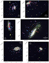 |
Fig. 1. RGB images of the six studied galaxies. The galaxies are JO201 and JO206 (top row), JW100 and JO204 (middle row), JW39 and JO175 (bottom row). The images are obtained following the prescription given in Gullieuszik et al. (2023) and summarized in Sect. 2. The white and black contours separate the tail, extraplanar, and disk regions, as described in Sect. 2.1. The white shaded area highlights the disk region, which is not considered throughout this work. The two contours almost coincide in JW39 and JO175 (bottom left and bottom right panels, respectively). The blue squares and red dots mark the position of UV and Hα leaf clumps with robust mass estimates (Giunchi et al. 2023a; Werle et al. 2024), summarized in Sects. 2.2 and 2.3. The pink arrow points towards the centre of the galaxy cluster (taken from Cava et al. 2009 and Biviano et al. 2017). |
The continuum emission in the F680N filter is interpolated from the adjacent filters (F606W and F814W) and subtracted in order to extract the intensity of the Hα line (either in emission or absorption).
2.1. Distinction of disk, extraplanar, and tail regions
As described in detail in Giunchi et al. (2023a), for each galaxy we defined three spatial categories to be studied separately: tail, extraplanar, and disk. The tail region is the area outside the most external layer of the optical stellar disk of the galaxy, defined as the 2σ contour (where σ is the background noise, computed as described in Gullieuszik et al. 2023) of the reddest photometric band available (F814W). Inside the optical stellar disk, we visually inspected the UV images (F275W + F336W) of the galaxies to define an inner contour separating clumps looking mostly undisturbed (disk clumps inside the contour) from those already showing clear signs of RPS, such as elongated and filamentary structures aligned with the stripping direction (extraplanar clumps outside the contour). The overlap of these clumps with the disk is most likely due to the combined effects of projection and their formation at very early stages of RPS when the gas had just been stripped and was still very close to the galaxy.
In Fig. 1 we show the contours defining the three spatial categories as white and black contours: the former traces the optical galactic disk; the latter divides clumps affected by RPS from those that appear undisturbed. The tail region includes everything outside the white contour; the extraplanar region is between the white and black contours; and the disk region is inside the black contour. We note that in some galaxies (namely JW39 and JO175, both in the bottom row of Fig. 1) the two contours are almost coincident since most of the clumps inside the optical galactic disk do not show signs of RPS.
2.2. Catalogue of star-forming clumps
In this section we summarize how the star-forming clumps and complexes were detected and selected, together with the main properties of the samples. For a complete description we refer to Giunchi et al. (2023a), in which the luminosity and size distribution functions and the luminosity-size relation of the clumps are studied.
The clumps are detected and selected independently in continuum-subtracted Hα-line and UV (F275W filter, ∼260 nm rest-frame at z = 0.05) images. Both of these tracers probe recently formed stars. Hα emission is due to gas ionized by very massive stars, and therefore probes star formation on timescales of ∼10 Myr, while UV emission is associated with the continuum of OBA stars, and therefore probes star formation on timescales of ∼200 Myr (Kennicutt 1998; Kennicutt & Evans 2012; Haydon et al. 2020). Using both tracers allows us to study how star formation in clumps changes both in time and space.
The clumps were selected using ASTRODENDRO2, a Python software package able to detect bright sources and, where present, also brighter sub-structures and secondary peaks within larger sources. The input parameters to be set include the minimum number of pixels that a clump candidate must possess, the minimum flux of each pixel, and the flux step used to search for bright sub-structures. In our case, we required a clump candidate to have at least five pixels (the minimum number of pixels needed to sample the PSF of HST), with a minimum flux of 2σ (where σ is the single-pixel detection limit, computed as described in Gullieuszik et al. 2023) and a flux step equal to 5σ. The resulting collection of structures was then catalogued as a hierarchical tree made of trunks and then nested into branches, finally reaching the top of the structures, known as leaves.
From the source sample detected by ASTRODENDRO, only candidates with a total signal-to-noise ratio S/N > 2 in at least three out of five photometric bands are kept. We used MUSE observations to confirm candidates in the tails and exclude background objects (see Poggianti et al. 2019b) by getting local redshift measurements from the corresponding spaxel, to be compared with that of the galaxy. Candidates outside of the MUSE field of view are confirmed if they have S/N > 2 in all the five photometric bands and positive Hα emission.
As described in detail in Giunchi et al. (2023a), for every clump a variety of physical parameters can be computed. The fluxes of the clumps in the five photometric filters are computed by integrating within their area, while their sizes are defined as twice the PSF-corrected core radius (rcore, corr). The core radius is the geometric mean of the semi-major and semi-minor axes of the clumps, which are the standard deviations of the surface brightness distribution of the clumps, computed along the direction of maximum elongation and the perpendicular direction, respectively. The photometric samples include 2406 Hα-selected clumps (1708 disk, 375 extraplanar, 323 tail) and 3745 UV-selected clumps (2021 disk, 825 extraplanar, 899 tail). As previously stated, throughout this paper we focus on the tail and extraplanar clumps.
2.3. Estimate of masses and ages of the clumps
Our aim for this work was the study of the mass function of the Hα- and UV-selected clumps observed in the tail and extraplanar regions of these galaxies; therefore, we needed the masses and (as we show in Appendix B) the ages of the clumps in the photometric catalogues described in the previous section. The procedure adopted to obtain stellar masses (M*) and mass-weighted ages (agemw) of the clumps is extensively described in Werle et al. (2024), and is briefly summarized here. Both those quantities were obtained using the Bayesian Analysis of Galaxies for Physical Inference and Parameter (BAGPIPES; Carnall et al. 2018), a code modelling the observed spectral energy distribution (SED), in our cases represented by the flux density in the five photometric filters.
First of all only leaf clumps with S/N > 2 in all the filters were selected. The code uses the 2016 update of the simple stellar population (SSP) models from Bruzual & Charlot (2003) with a Kroupa (2001) IMF; the solar metallicity is assumed to be Z⊙ = 0.017. Adopting a Bayesian fitting technique, BAGPIPES returns posterior probability distributions (PDFs) for each fitted quantity; in the following, the reference value of a physical property is computed as the median of its PDF. Clump star formation histories (SFHs) were modelled as a single delayed exponential (Carnall et al. 2019).
In the case of stellar populations younger than 20 Myr, the code includes emission lines and nebular continuum emission from CLOUDY (Ferland et al. 2017). Dust was modelled after the Milky Way extinction curve from Cardelli et al. (1989), assuming RV = 3.1 and two foreground dust screens with different V-band extinction AV, for stellar populations older and younger than 20 Myr, respectively. The young-to-old AV ratio was kept between 1 and 2.5. The total assembled stellar mass was left to vary from 0 to 1010 M⊙ and the ages between 0 and 500 Myr.
The resulting fits underwent a series of quality-check controls. To evaluate how the underlying stellar populations belonging to the galaxy disk might affect our results (especially for extraplanar clumps), a SFH with two components was tested to model both the young and old stellar populations. If the addition of a second component led to unconstrained mass and age, or if the old component was found to be more than 100 times more massive than the young one, the clump was discarded, as in both cases the properties of the young stellar populations could not be constrained well enough. This happens for ∼7% (∼16%) of the Hα (UV) clumps (mostly in the extraplanar region). For ∼8% of the Hα clumps and ∼22% of the UV clumps the model fluxes are outside the 2σ error bars of the observations for one or more filters; the fit thus cannot be considered satisfactory, and is therefore discarded.
After these quality-check cuts our final sample consists of 398 Hα-selected clumps (188 tail, 210 extraplanar) and 1270 UV-selected clumps (593 tail, 677 extraplanar). The clump positions are plotted in Fig. 1 as red dots and blue squares for the Hα and UV clumps, respectively. The distributions of the stellar mass and mass-weighted ages of the Hα and UV clumps, also divided into tail and extraplanar regions, are shown in Fig. 2. Our masses span a large interval going from a few 103 M⊙ up to 108 M⊙. The most massive clumps in the sample are located in the extraplanar region, while the low-mass regime is populated by the Hα clumps, whether in tails or extraplanar regions. The ages go from a few megayears to hundreds of megayears, with the youngest clumps preferentially selected in Hα and the oldest ones in UV. A detailed study of these mass and age distributions was performed by Werle et al. (2024).
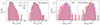 |
Fig. 2. Stellar mass (top row) and mass-weighted age (bottom row) distributions of Hα (red histograms) and UV (blue histograms) clumps. The clumps were divided into tail (left panels) and extraplanar (right panels) according to the criteria described in Sect. 2.1, and the sample was selected following the procedure described in Sect. 2.3. |
3. Modelling the mass function
Before fitting a chosen function to the clump mass distribution, we needed to quantify the main sources of bias and uncertainty that could lead to incorrect results. We considered two effects: the completeness of the sample as a function of the clump mass, and the bias and uncertainty on the estimate of the intrinsic mass of a clump, which highly depends on how the fluxes are computed and on the model adopted for the SED fitting.
One way to quantify these effects is to study images of mock clumps with given mass and age as if they were real images, comparing the input quantities with those retrieved as output, similarly to what has been done for other surveys of extended objects (Villegas et al. 2010; Sun et al. 2024). In order to do this, we modelled the morphology and SED of the clumps as a function of their mass and age and, based on these models, generated the library of mock images. The age of the clumps determines the shape of the SED and the mass-to-light ratio, while the mass of the clumps constrains the bolometric luminosity (fixed the mass-to-light ratio) and the size. Further details about how this library was created is given in Appendix, from A to E, and is briefly summarized here:
-
We stacked a sub-sample of resolved clumps, characterized by smooth, round, non-peculiar morphology and properly normalized in size and flux in order to be comparable with each other. The stacked image was then fitted to two 2D Moffat functions, producing the stacked model, fully normalized both in size and flux. This was done independently for the Hα and UV clumps.
-
The clump masses were extracted from a flat distribution (in order to evenly sample and study all the mass regimes), while the ages followed the observed age distribution derived as described in Sect. 2.3.
-
The physical size of the clump was derived for a given mass from the clump size-mass relation (fitted as described in Sect. C).
-
The shape of the SED was determined by the age of the clumps, which determines for example how bright the Hα line or the UV part of the spectrum is. In particular, we adopted the resulting SEDs obtained from the fits performed with BAGPIPES in Werle et al. (2024);
-
Finally, for a given age, the mass-to-light ratio determines the flux normalization of the SED.
We note that the steps listed above were performed independently for the four sub-samples (Hα tail, Hα extraplanar, UV tail, and UV extraplanar clumps) that can possibly have different size-mass relations, age distributions, and mass-to-light ratios. The only exception is step 1 (i.e. the generation of the stacked clump model), which is performed separately for the Hα and UV clumps, but with no further divisions related to the spatial category.
The subsequent step is described in detail in Appendix E and consists in adding the mock clumps to the real images, on which we performed the same procedure adopted to detect the real clumps (Giunchi et al. 2023a, summarized in Sect. 2.2) and obtained their masses (Werle et al. 2024, summarized in Sect. 2.3). This process was iterated many times in order to reach a sufficient level of statistics (∼1000 mock clumps per galaxy). The number of clumps added to the tail and extraplanar regions at each iteration was set by the need not to change the crowding of the real underlying clump population of the studied galaxy. Whether the mock clump is re-detected or not (and if detected the comparison between input and output properties) quantify the aforementioned sources of uncertainty. In the following sections we show in detail the results for the completeness (Sect. 3.1) and the mass bias (Sect. 3.2).
3.1. Completeness
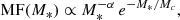
We define the completeness as the fraction of re-detected clumps per intrinsic mass. We modelled it as a logistic function characterized by an S-shaped curve, monotonically increasing from one asymptotic value (for x → −∞) to another (for x → +∞). The equation describing the logistic function (McCullagh & Nelder 1989; Peng et al. 2002) is
![$$ \begin{aligned} C(\log m_{\rm in})=\frac{k}{[1+e^{-p(\log m_{\rm in}-\log m_{\rm in,0})}]}, \end{aligned} $$](/articles/aa/full_html/2025/04/aa52983-24/aa52983-24-eq15.gif)
where min is the intrinsic mass, k is the value of the asymptotic value for min → +∞, p regulates the sharpness of the increase of the function, and min, 0 is the scale intrinsic mass at which C(log min, 0) = k/(1 + e).
The space of the free parameters (k, p, log min, 0) is explored according to the log-likelihood function of the logistic regression (McCullagh & Nelder 1989; Peng et al. 2002)
![$$ \begin{aligned} \log \mathcal{L} _C=\sum _{i=1}^{N_{\rm det}}\log C(\log m_{\mathrm{in},i})+\sum _{j=1}^{N_{\rm non-det}}\log [1-C(\log m_{\mathrm{in},j})], \end{aligned} $$](/articles/aa/full_html/2025/04/aa52983-24/aa52983-24-eq16.gif)
where Ndet and Nnon − det are the numbers of re-detected and non-detected mock clumps added to the mock observations, respectively, while min, i and min, j are the input stellar masses of the i-th re-detected and j-th non-detected mock clumps, respectively. We computed the best-fitting parameters as the median of the PDFs obtained by exploring the parameter space to maximize ℒC and listed in rows (2)–(4) in Table 2. We note that the fitting procedure we followed (Eq. (3)) is binning independent.
Best-fitting parameters of the completeness and mass bias functions for the Hα tail (first row), Hα extraplanar (second row), UV tail (third row), and UV extraplanar (fourth row) mock clumps.
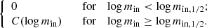
Correcting for the non-detected clumps when the completeness is below 0.5, where more than half of the clumps are lost, may not lead to robust estimates. Therefore, we force the completeness to 0 for input masses below the value min, 1/2 at which C(log min, 1/2) = 0.5. The operative completeness  becomes
As an example, in the left panel of Fig. 3 we show the Hα tail completeness function (where the dashed line is the profile of C(log min) before forcing it to 0). For a visual comparison, we over-plotted the observed input mass completeness; this is computed by binning the mock clumps in input mass, assigning to the k-th bin a value Ck = Ndet, k/Nk, where Nk and Ndet, k are the total number and the number of re-detected clumps in the k-th bin, respectively. The same plots for the other filters and regions are shown in the left panels of Fig. F.1, showing that the best-fitting functions well reproduce the results from the mock observations, with low-mass clumps more likely to be lost, as expected.
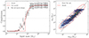 |
Fig. 3. Completeness (left) and mass estimation bias (right) for Hα tail clumps. In the left panel the red solid line is the best-fitting model computed as in Eq. (4), cut to 0 for values below 0.5 (Sect. 3.1), while the red dashed line shows the uncut function. The threshold value of 0.5, below which the function is forced to 0, is plotted as a grey dotted line. The black empty circles show the binned mass completeness derived from the mock clumps (with uncertainties equal to the Poissonian error), for a qualitative visualization of the goodness of the fit (the fitting technique does not depend on the binning). The right panel shows the relationship between the observed (x-axis) and intrinsic (y-axis) mass for the Hα tail re-detected mock clumps. Each clump is plotted as a blue dot. The black dashed line is the 1:1 relation. The red contours are computed from the best-fitting model describing the clumps distribution (Eq. (5)). |
3.2. Mass estimate bias
Our capability of recovering the intrinsic mass of a star-forming clump is affected by many factors, for example the noise of the image, which especially affects the faint regions of the clump, the definition of clump flux (Giunchi et al. 2023a), and the models used to infer the mass (Werle et al. 2024). The comparison between the intrinsic mass of the mock clumps and the observed value can quantify this effect and reveal the presence of systematics.
In the right panel of Fig. 3 we show the comparison between observed and intrinsic mass of the re-detected Hα tail mock clumps. We note that for high masses there is a good agreement between them, while at low masses the observed mass is systematically lower than the intrinsic value. Similar plots for the different filters and regions (UV tail, Hα extraplanar, and UV extraplanar, respectively) are shown in Fig. F.1, which show how the underlying disk strongly increases the uncertainties on the mass estimate in the extraplanar region.
We modelled the distribution of (log mobs, log min) as a quadratic relation F with linearly decreasing scatter σ depending on the observed mass log mobs:
![$$ \begin{aligned} {\left\{ \begin{array}{ll} F(\log m_{\rm obs}) =&a+b\cdot \log m_{\rm obs}+c\cdot (\log m_{\rm obs})^2+\\&+g[0,\sigma (\log m_{\rm obs})] \\ \sigma (\log m_{\rm obs}) =&d+e\cdot \log m_{\rm obs} \end{array}\right.}. \end{aligned} $$](/articles/aa/full_html/2025/04/aa52983-24/aa52983-24-eq19.gif)
The best-fitting values of the free parameters (a, b, c, d, e) are the median values of the PDFs obtained sampling the parameter space of the log-likelihood (Ponomareva et al. 2017; Posti et al. 2018; Bacchini et al. 2019)
![$$ \begin{aligned} \log \mathcal{L} _{\rm bias}=-\frac{1}{2}\sum _{i=1}^{N_{\rm cl}}\left[ \frac{d_i^2}{\sigma _{\rm tot}^2} + \ln (2\pi \sigma _{\rm tot}^2) \right], \end{aligned} $$](/articles/aa/full_html/2025/04/aa52983-24/aa52983-24-eq20.gif)
where Ncl is the number of re-detected mock clumps, di2 = log min, i2 − [a + b ⋅ log mobs, i + c ⋅ (log mobs)2]2 is the distance between the i-th intrinsic mass and that inferred from the model, and σtot = σ(log mobs, i) is the intrinsic scatter at the i-th observed mass. The uncertainty on the mass estimate given by BAGPIPES is neglected a posteriori since it is much smaller than the intrinsic scatter obtained by this fit. The best-fitting parameters are listed in the last five columns of Table 2, and the model distributions are shown as contours in Fig. 3 (and for the other filters and regions in Fig. F.1), where they describe the mock clump distributions well.
Thanks to this model, at a given j-th clump observed mass log mobs, j we define a Gaussian distribution Gj(log min) with mean and standard deviation given by Eq. (5), which describes the distribution of possible intrinsic masses that can result in the observed mass log mobs, j.
3.3. Modelling the mass function
The fitting to the mass function (MF) must take into account the effects that we quantify in the previous sections; the number of clumps with a certain mass affected by incompleteness and a clump with a given observed mass may have a different input mass, which is the real value on which the MF depends. The likelihood we used to explore the parameter space is taken from Vasiliev (2019), which was applied in a different context (fitting a sample of globular clusters to a distribution function) but with the same ingredients we have considered. The functional form of the log-likelihood is
where Ncl is the number of real UV or Hα clumps with reliable mass estimates (Sect. 2.3), ω = log min (the clump intrinsic mass), MF(ω, θ) is the mass function with free parameters θ (the functional form is described below), π(θ) is the prior of the parameters (which depends on the parameters of the MF), Gi(ω) is the input mass distribution of the i-th observed mass log mobs, i (Sect. 3.2), and  is the completeness (Sect. 3.1). We note that the integral over input masses is done only for values larger than log min, 1/2, avoiding a mass regime in which the fit is highly affected by incompleteness.
4. Results
As stated in Sect. 1, whether the clump mass functions present a high-mass cut-off and what drives the value of this mass cut-off are still highly debated in literature. In order to test the putative presence of a cut-off mass in our sample, in the following sections we fit our clump mass datasets to a single power law and to a Schechter function.
4.1. Fit of the mass function to a single power law
We fitted the observed data to a MF modelled as a single power law (Eq. (1)), with only the slope α as a free parameter. The best-fitting slopes were computed as the median values of the parameter distributions, while the uncertainties are the 84th percentile minus the median and the median minus the 16th percentile (upper and lower uncertainty, respectively). For the tail clumps the retrieved slopes are 2.31 ± 0.12 in Hα and 2.60 ± 0.09 in UV. In the extraplanar region, the best-fitting slopes are  and
and  in Hα and UV, respectively. The posterior distributions are shown in Fig. 4.
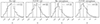 |
Fig. 4. Posterior distribution of the slope parameters α, inferred fitting a power law to the mass distribution of tail clumps (first two panels) and extraplanar clumps (last two panels). Hα is on the left, and UV is on the right. The vertical dashed black lines are the 16th, 50th, and 84th percentiles, also reported in the legends. |
Our slope values are all more than 1σ larger than the typical value found in the literature (α = 2.0 ± 0.2, Krumholz et al. 2019); the only exception is the tail Hα clumps. Such large slopes are usually associated with environmental effects and variations in the SFR surface density ΣSFR. The environment in which jellyfish galaxies are located and the effects of RPS could halt the formation of massive clumps and explain the steepening. In Sect. 4.2 we test our results adopting different MF functional models, while in Sect. 5 we further discuss the possible causes of the steepness of the observed mass function.
The slope of the tail UV mass function is steeper (at 2σ confidence level), and therefore compatible with models predicting this evolution of the slope as a function of the ageing and dynamical evolution of the clumps (Fujii & Portegies Zwart 2015).
In the extraplanar region, Hα clumps show a steeper slope than in the tail regions (yet consistent within 1σ), hinting that the formation of massive clumps is even more halted under these conditions, possibly as a consequence of ram pressure, which is causing both gas compression and stripping, which are both at very early stages in this region where the gas is still very close to the disk. Similarly to tail clumps, in the extraplanar region the UV mass function is also steeper than the Hα, even though the slope is identical to that in the tail. However, we note that they are consistent within 1σ. In the following section we discuss in more detail the behaviour and the observational caveats that are present when working in the extraplanar region. As a consequence, the values of the slopes for the extraplanar clumps should be taken with caution.
4.2. Fit of the mass function to a Schechter function
We explored the case of the Schechter function fitting instead of the simple power law. The Schechter function is defined as (Schechter 1976)
with the slope α and the cut-off mass Mc. As described in Appendix G, our fitting procedure is able to rule out or not the presence of a cut-off mass even when a small sample (about 100 clumps) is fitted. Therefore, this is a good test to confirm whether the observed mass function is a power law.
The parameter space is explored using the same procedure described in Sect. 3.3 and just changing the functional form of the mass function. The results are shown in corner plots of Fig. 5 for the tail and the extraplanar clumps (Hα and UV).
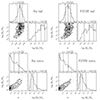 |
Fig. 5. Corner plots of the parameter space (α, log Mc) (the slope and the cut-off mass, respectively), obtained fitting a Schechter mass function (Eq. (8)) to the Hα and UV tail (top row) and extraplanar (bottom row) clump mass distribution. The values at the top of the histograms are the median of each distribution for the corresponding parameter, with uncertainties given by the 84th percentile minus the median and the median minus the 16th percentile (upper and lower uncertainty, respectively). The same values are also reported as black dashed vertical lines in the histograms. |
In the tails the cut-off mass is unconstrained and peaks at masses higher than 107 M⊙, while the best-fitting MF slopes are  and 2.54 ± 0.12 for Hα and UV clumps, respectively. Both slopes are consistent with the values obtained when fitting a single power law (Sect. 4.1), even though systematically smaller. On the other hand, in the extraplanar region both the slopes of the Hα and UV clumps have unconstrained results, for which we can only set an upper limit α ≲ 2, while the cut-off masses are constrained with
 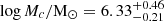 and
and  for the Hα and the UV samples, respectively. By comparing the shape of the contours and the constraints on the parameters, for the tail clumps (either Hα or UV) we can rule out the presence of a cut-off mass, for which only a lower limit can be set and at values larger than the most massive clumps of the sample. This suggests that the most correct shape for the tail mass function is a simple power law.
For the extraplanar regions, the fit suggests the presence of a cut-off that is well constrained and at values comparable with the fitted mass interval. However, no constraints can be put on the slope, for which the fit sets an upper limit. Furthermore, we performed the Bayesian information criterion (BIC) test (Wit & Heuvel 2012) to quantify whether the addition of a cut-off mass concretely improves the goodness of the fit. The BIC of a model is defined as (Wit & Heuvel 2012)
where k is the number of free parameters of the model, n is the number of data points, and ℒ is the likelihood of the model. In our case, the BIC differences ΔBIC between the power law and the Schechter cases are always smaller than 2; therefore, there is no strong evidence that the Schechter function is a better model than the power law.
The difficulty in constraining the parameters of the extraplanar clumps is most likely due to a series of caveats that become negligible when moving to the tails. The underlying old stellar disk and the large blending rate (even in the outskirts of disks) make it non-trivial to correctly estimate the stellar mass of the clumps, which are characterized by larger uncertainties and a poor completeness. Both these effects are extensively discussed and quantified in the previous sections (Sects. 3.2 and 3.1), but deeper observations are needed to improve the fit in the extraplanar region by extending the range of fitted masses, including the power-law regime. Considering that the BIC test ruled out the need of the Schechter function, we present in the previous section the values of the slopes obtained from the fit to a power law. Even so, the resulting slopes for extraplanar clumps are dependent on the fitted mass range and to the aforementioned observational caveats.
5. Discussion and conclusion
Throughout this paper we have shown our results for the mass distribution functions of a sample of star-forming clumps in a set of six galaxies undergoing strong ram-pressure stripping. The clumps were selected both in Hα and UV, and divided into two spatial categories: tail, if observed far away from the galactic plane, and extraplanar, if the clump is in the outskirts of the galactic disk but already showing the signs of ram-pressure stripping.
The fit of the mass functions of these sub-samples of clumps was performed by means of a Bayesian algorithm, which let us fit the distribution in a way that is binning-independent. By modelling our clumps and performing a set of mock observations, we also quantified the mass completeness and bias of the sub-samples, showing how these observational effects can highly affect the steepness of the observed mass function. Not taking into account these effects lead to shallower mass distributions, in turn leading to completely different conclusions and interpretations. Therefore, we improved our results with respect to our previous study on the luminosity function of these objects (Giunchi et al. 2023a). Our findings are as follows:
-
The mass function of the tail clumps is better described by a power law rather than a Schechter function. Having ruled out the presence of a cut-off mass, our slopes are steeper than the value α = 2 typically obtained from observations (Krumholz et al. 2019) and simulations (Renaud et al. 2024) of main-sequence isolated galaxies, and equal to 2.31 ± 0.12 in Hα and 2.60 ± 0.09 in UV. This difference is remarkable: in Giunchi et al. (2023a) it was shown that clumps in jellyfish galaxies are likely to be experiencing an enhancement in star formation rate surface density (ΣSFR), similarly to star-forming clumps in starburst galaxies (Fisher et al. 2017), as hinted by the observed enhancement in Hα luminosity. Previous works have shown that the mass function of young clumps in such environments (also including spiral arms, for instance) is shallower than in main-sequence isolated galaxies or in the inter-arm regions of spiral galaxies, and therefore the formation of massive clumps is favoured. Nonetheless, our sample of clumps, although enhanced in ΣSFR, show large slopes, usually associated with regions with mild star formation, for example the inter-arm regions of spiral-armed galaxies (Haas et al. 2008; Messa et al. 2018, 2019);
-
In the extraplanar region the resulting slopes are
 in Hα and
  in UV. The extraplanar Hα mass function is steeper than the tail mass function. Furthermore, similarly to the tail region, also for the extraplanar clumps the UV mass function is steeper than the Hα mass function. However, the uncertainties on the extraplanar slopes are such that they are all consistent within 1σ, making it difficult to draw strong conclusions. Further tests on the clumps of this region suggest that a cut-off mass, which could bias the inferred value of the slope, is likely to the present, even if the depth of the sample and the observational caveats in this regions make it difficult to put strong constraints on both parameters, and statistical tests rule out the need of a second parameter.
The unpredicted steepening of our mass function has never been observed in galaxies with enhanced ΣSFR (Livermore et al. 2012) and not even in the tidal tails of merging galaxies (Rodruck et al. 2023); therefore, it must be closely connected to the peculiar environment experienced by the clumps in the tails of these jellyfish galaxies, far away from the galactic disk and embedded in the hot and high-pressure ICM. In this context, recent works by Li et al. (2023) and Ignesti et al. (2024) studied the mixing between the stripped ISM and the surrounding ICM by means of the velocity structure function (VSF), which is a two-point correlation function that quantifies the kinetic energy fluctuations as a function of the scale l in a velocity field. The former focused on the RPS galaxy ESO 137-001; the latter studied ten galaxies from the GASP survey, extending the study of the ICM turbulence to galaxies of different masses and RPS stage and included five of the six galaxies from this work (with the exception of JO201). In both works, the VSFs suggest that the mixing of these two gas phases triggers the Kelvin-Helmholtz instability that induces turbulent motions down to scales as small as 0.2 kpc, regardless of the studied galaxies. The presence of turbulent motions on scales larger than 1 kpc implies that the collapse of large and massive clumps is hindered by the contribution of turbulence to the gas internal pressure. Furthermore, Li et al. (2023) have found that turbulent motions triggered by the ICM increase with the distance from the disk. Therefore the formation of massive clumps is even more halted in the tails, explaining why the most massive clumps in our samples are located in the extraplanar region (Sect. 2.3 and Fig. 2).
It is worth noting that the interaction between ISM and ICM also involves other processes (Ge et al. 2021) not addressed by the afore-mentioned studies, such as thermal heating (because of mixing, thermal conduction, and radiative heating, Campitiello et al. 2021) and magnetic fields, which can either prevent or favour gas collapse (Müller et al. 2021a,b). These phenomena can affect the gas collapse and the properties of the clumps; however, their net effects are still debated due to the complexity of the processes at play.
Our results suggest that star formation is highly sensitive to the environment in which it occurs. Increasing the available statistics of highly resolved clumps, in combination with multi-wavelength observations focusing on the gaseous components, would improve our understanding of the star formation process.
Acknowledgments
We thank the anonymous referee for their useful comments that helped to improve this script. EG would like to thank the GASP team, Raffaele Pascale, Carlo Nipoti and Alessandro Della Croce for the useful discussions and comments. The research activities described in this paper have been co-funded by the European Union – NextGenerationEU within PRIN 2022 project n.20229YBSAN – Globular clusters in cosmological simulations and in lensed fields: from their birth to the present epoch. This paper is based on observations made with the NASA/ESA Hubble Space Telescope obtained from the Space Telescope Science Institute, which is operated by the Association of Universities for Research in Astronomy, Inc., under NASA contract NAS 5-26555. These observations are under the programme GO-16223. All the HST data used in this paper can be found in MAST: http://dx.doi.org/10.17909/tms2-9250. This paper used also observations collected at the European Organization for Astronomical Research in the Southern Hemisphere associated with the ESO programme 196.B-0578. This research made use of Astropy, a community developed core Python package for Astronomy by the Astropy Collaboration (2018). This project has received funding from the European Research Council (ERC) under the European Union’s Horizon 2020 research and innovation programme (grant agreement No. 833824). We acknowledge support from the INAF Minigrant “Clumps at cosmological distance: revealing their formation, nature, and evolution” (Ob. Fu. 1.05.23.04.01).
References
- Abramson, A., & Kenney, J. D. P. 2014, AJ, 147, 63 [Google Scholar]
- Adamo, A., Ryon, J. E., Messa, M., et al. 2017, ApJ, 841, 131 [Google Scholar]
- Astropy Collaboration (Price-Whelan, A. M., et al.) 2018, AJ, 156, 123 [Google Scholar]
- Audit, E., & Hennebelle, P. 2010, A&A, 511, A76 [NASA ADS] [CrossRef] [EDP Sciences] [Google Scholar]
- Bacchini, C., Fraternali, F., Iorio, G., & Pezzulli, G. 2019, A&A, 622, A64 [NASA ADS] [CrossRef] [EDP Sciences] [Google Scholar]
- Bellhouse, C., Jaffé, Y. L., Hau, G. K. T., et al. 2017, ApJ, 844, 49 [NASA ADS] [CrossRef] [Google Scholar]
- Bellhouse, C., Jaffé, Y. L., McGee, S. L., et al. 2019, MNRAS, 485, 1157 [Google Scholar]
- Bellhouse, C., McGee, S. L., Smith, R., et al. 2021, MNRAS, 500, 1285 [Google Scholar]
- Biviano, A., Moretti, A., Paccagnella, A., et al. 2017, A&A, 607, A81 [NASA ADS] [CrossRef] [EDP Sciences] [Google Scholar]
- Boselli, A., Fossati, M., & Sun, M. 2022, A&ARv, 30, 3 [NASA ADS] [CrossRef] [Google Scholar]
- Bressert, E., Bastian, N., Gutermuth, R., et al. 2010, MNRAS, 409, L54 [NASA ADS] [Google Scholar]
- Bruzual, G., & Charlot, S. 2003, MNRAS, 344, 1000 [NASA ADS] [CrossRef] [Google Scholar]
- Calzetti, D., Lee, J. C., Sabbi, E., et al. 2015, AJ, 149, 51 [Google Scholar]
- Campitiello, M. G., Ignesti, A., Gitti, M., et al. 2021, ApJ, 911, 144 [NASA ADS] [CrossRef] [Google Scholar]
- Cardelli, J. A., Clayton, G. C., & Mathis, J. S. 1989, ApJ, 345, 245 [Google Scholar]
- Carnall, A. C., McLure, R. J., Dunlop, J. S., & Davé, R. 2018, MNRAS, 480, 4379 [Google Scholar]
- Carnall, A. C., Leja, J., Johnson, B. D., et al. 2019, ApJ, 873, 44 [Google Scholar]
- Cava, A., Bettoni, D., Poggianti, B. M., et al. 2009, A&A, 495, 707 [NASA ADS] [CrossRef] [EDP Sciences] [Google Scholar]
- Consolandi, G., Gavazzi, G., Fossati, M., et al. 2017, A&A, 606, A83 [NASA ADS] [CrossRef] [EDP Sciences] [Google Scholar]
- Cortese, L., Catinella, B., & Smith, R. 2021, PASA, 38, e035 [NASA ADS] [CrossRef] [Google Scholar]
- Cramer, W. J., Kenney, J. D. P., Sun, M., et al. 2019, ApJ, 870, 63 [Google Scholar]
- de Grijs, R., & Anders, P. 2006, MNRAS, 366, 295 [CrossRef] [Google Scholar]
- de Grijs, R., Anders, P., Bastian, N., et al. 2003, MNRAS, 343, 1285 [NASA ADS] [CrossRef] [Google Scholar]
- Deb, T., Verheijen, M. A. W., Gullieuszik, M., et al. 2020, MNRAS, 494, 5029 [Google Scholar]
- Elmegreen, B. G. 2002, ApJ, 564, 773 [NASA ADS] [CrossRef] [Google Scholar]
- Elmegreen, B. G. 2006, ApJ, 648, 572 [Google Scholar]
- Fensch, J., Bournaud, F., Brucy, N., et al. 2023, A&A, 672, A193 [NASA ADS] [CrossRef] [EDP Sciences] [Google Scholar]
- Ferland, G. J., Chatzikos, M., Guzmán, F., et al. 2017, Rev. Mex. Astron. Astrofis., 53, 385 [NASA ADS] [Google Scholar]
- Fisher, D. B., Glazebrook, K., Damjanov, I., et al. 2017, MNRAS, 464, 491 [CrossRef] [Google Scholar]
- Foreman-Mackey, D., Hogg, D. W., Lang, D., & Goodman, J. 2013, PASP, 125, 306 [Google Scholar]
- Fossati, M., Fumagalli, M., Boselli, A., et al. 2016, MNRAS, 455, 2028 [Google Scholar]
- Franchetto, A., Vulcani, B., Poggianti, B. M., et al. 2020, ApJ, 895, 106 [NASA ADS] [CrossRef] [Google Scholar]
- Fritz, J., Moretti, A., Gullieuszik, M., et al. 2017, ApJ, 848, 132 [NASA ADS] [CrossRef] [Google Scholar]
- Fujii, M. S., & Portegies Zwart, S. 2015, MNRAS, 449, 726 [NASA ADS] [CrossRef] [Google Scholar]
- Ge, C., Luo, R., Sun, M., et al. 2021, MNRAS, 505, 4702 [NASA ADS] [CrossRef] [Google Scholar]
- George, K., Poggianti, B. M., Gullieuszik, M., et al. 2018, MNRAS, 479, 4126 [Google Scholar]
- George, K., Poggianti, B. M., Bellhouse, C., et al. 2019, MNRAS, 487, 3102 [Google Scholar]
- George, K., Poggianti, B. M., Tomičić, N., et al. 2023, MNRAS, 519, 2426 [Google Scholar]
- Gieles, M. 2009, Ap&SS, 324, 299 [Google Scholar]
- Gieles, M., Larsen, S. S., Scheepmaker, R. A., et al. 2006, A&A, 446, L9 [NASA ADS] [CrossRef] [EDP Sciences] [Google Scholar]
- Giunchi, E., Gullieuszik, M., Poggianti, B. M., et al. 2023a, ApJ, 949, 72 [NASA ADS] [CrossRef] [Google Scholar]
- Giunchi, E., Poggianti, B. M., Gullieuszik, M., et al. 2023b, ApJ, 958, 73 [NASA ADS] [CrossRef] [Google Scholar]
- Göller, J., Joshi, G. D., Rohr, E., Zinger, E., & Pillepich, A. 2023, MNRAS, 525, 3551 [CrossRef] [Google Scholar]
- Gullieuszik, M., Poggianti, B. M., Moretti, A., et al. 2017, ApJ, 846, 27 [Google Scholar]
- Gullieuszik, M., Giunchi, E., Poggianti, B. M., et al. 2023, ApJ, 945, 54 [NASA ADS] [CrossRef] [Google Scholar]
- Gunn, J. E., Gott, J., & Richard, I. 1972, ApJ, 176, 1 [Google Scholar]
- Haas, M. R., Gieles, M., Scheepmaker, R. A., Larsen, S. S., & Lamers, H. J. G. L. M. 2008, A&A, 487, 937 [NASA ADS] [CrossRef] [EDP Sciences] [Google Scholar]
- Haydon, D. T., Kruijssen, J. M. D., Chevance, M., et al. 2020, MNRAS, 498, 235 [NASA ADS] [CrossRef] [Google Scholar]
- Hennebelle, P., & Audit, E. 2007, A&A, 465, 431 [NASA ADS] [CrossRef] [EDP Sciences] [Google Scholar]
- Hunter, D. A., Elmegreen, B. G., Dupuy, T. J., & Mortonson, M. 2003, AJ, 126, 1836 [NASA ADS] [CrossRef] [Google Scholar]
- Ignesti, A., Vulcani, B., Poggianti, B. M., et al. 2022a, ApJ, 924, 64 [NASA ADS] [CrossRef] [Google Scholar]
- Ignesti, A., Vulcani, B., Poggianti, B. M., et al. 2022b, ApJ, 937, 58 [NASA ADS] [CrossRef] [Google Scholar]
- Ignesti, A., Brunetti, G., Gullieuszik, M., et al. 2024, ApJ, 977, 219 [Google Scholar]
- Jáchym, P., Kenney, J. D. P., Sun, M., et al. 2019, ApJ, 883, 145 [Google Scholar]
- Kelly, B. C. 2007, ApJ, 665, 1489 [Google Scholar]
- Kenney, J. D. P., Abramson, A., & Bravo-Alfaro, H. 2015, AJ, 150, 59 [Google Scholar]
- Kennicutt, R. C., Jr. 1998, ARA&A, 36, 189 [Google Scholar]
- Kennicutt, R. C., & Evans, N. J. 2012, ARA&A, 50, 531 [NASA ADS] [CrossRef] [Google Scholar]
- Krist, J. E., Hook, R. N., & Stoehr, F. 2011, in Optical Modeling and Performance Predictions V, ed. M. A. Kahan, Society of Photo-Optical Instrumentation Engineers (SPIE) Conference Series, 8127, 81270J [Google Scholar]
- Kroupa, P. 2001, MNRAS, 322, 231 [NASA ADS] [CrossRef] [Google Scholar]
- Krumholz, M. R., McKee, C. F., & Bland-Hawthorn, J. 2019, ARA&A, 57, 227 [NASA ADS] [CrossRef] [Google Scholar]
- Lada, C. J., & Lada, E. A. 2003, ARA&A, 41, 57 [Google Scholar]
- Lee, J. C., Whitmore, B. C., Thilker, D. A., et al. 2022, ApJS, 258, 10 [NASA ADS] [CrossRef] [Google Scholar]
- Li, Y., Luo, R., Fossati, M., Sun, M., & Jáchym, P. 2023, MNRAS, 521, 4785 [NASA ADS] [CrossRef] [Google Scholar]
- Livermore, R. C., Jones, T., Richard, J., et al. 2012, MNRAS, 427, 688 [NASA ADS] [CrossRef] [Google Scholar]
- McCullagh, P., & Nelder, J. 1989, Generalized Linear Models (Chapman and Hall) [CrossRef] [Google Scholar]
- Merluzzi, P., Busarello, G., Dopita, M. A., et al. 2013, MNRAS, 429, 1747 [Google Scholar]
- Messa, M., Adamo, A., Östlin, G., et al. 2017, MNRAS, 473, 996 [Google Scholar]
- Messa, M., Adamo, A., Calzetti, D., et al. 2018, MNRAS, 477, 1683 [NASA ADS] [CrossRef] [Google Scholar]
- Messa, M., Adamo, A., Östlin, G., et al. 2019, MNRAS, 487, 4238 [NASA ADS] [CrossRef] [Google Scholar]
- Moretti, A., Paladino, R., Poggianti, B. M., et al. 2018, MNRAS, 480, 2508 [Google Scholar]
- Moretti, A., Paladino, R., Poggianti, B. M., et al. 2020, ApJ, 889, 9 [Google Scholar]
- Müller, A., Poggianti, B. M., Pfrommer, C., et al. 2021a, Nature, 5, 159 [Google Scholar]
- Müller, A., Pfrommer, C., Ignesti, A., et al. 2021b, MNRAS, 508, 5326 [CrossRef] [Google Scholar]
- Peluso, G., Vulcani, B., Poggianti, B. M., et al. 2022, ApJ, 927, 130 [NASA ADS] [CrossRef] [Google Scholar]
- Peng, C.-Y. J., Lee, K. L., & Ingersoll, G. M. 2002, J. Educ. Res., 96, 3 [Google Scholar]
- Poggianti, B. M., Fasano, G., Omizzolo, A., et al. 2016, AJ, 151, 78 [Google Scholar]
- Poggianti, B. M., Jaffé, Y. L., Moretti, A., et al. 2017a, Nature, 548, 304 [Google Scholar]
- Poggianti, B. M., Moretti, A., Gullieuszik, M., et al. 2017b, ApJ, 844, 48 [Google Scholar]
- Poggianti, B. M., Ignesti, A., Gitti, M., et al. 2019a, ApJ, 887, 155 [Google Scholar]
- Poggianti, B. M., Gullieuszik, M., Tonnesen, S., et al. 2019b, MNRAS, 482, 4466 [Google Scholar]
- Ponomareva, A. A., Verheijen, M. A. W., Peletier, R. F., & Bosma, A. 2017, MNRAS, 469, 2387 [NASA ADS] [CrossRef] [Google Scholar]
- Portegies Zwart, S. F., McMillan, S. L. W., & Gieles, M. 2010, ARA&A, 48, 431 [NASA ADS] [CrossRef] [Google Scholar]
- Posti, L., Fraternali, F., Di Teodoro, E. M., & Pezzulli, G. 2018, A&A, 612, L6 [NASA ADS] [CrossRef] [EDP Sciences] [Google Scholar]
- Radovich, M., Poggianti, B., Jaffé, Y. L., et al. 2019, MNRAS, 486, 486 [Google Scholar]
- Ramatsoku, M., Serra, P., Poggianti, B. M., et al. 2020, A&A, 640, A22 [NASA ADS] [CrossRef] [EDP Sciences] [Google Scholar]
- Renaud, F., Agertz, O., & Romeo, A. B. 2024, A&A, 687, A91 [NASA ADS] [CrossRef] [EDP Sciences] [Google Scholar]
- Rodruck, M., Charlton, J., Borthakur, S., et al. 2023, MNRAS, 526, 2341 [Google Scholar]
- Schechter, P. 1976, ApJ, 203, 297 [Google Scholar]
- Smith, R. J., Lucey, J. R., Hammer, D., et al. 2010, MNRAS, 408, 1417 [Google Scholar]
- Sun, M., Ge, C., Luo, R., et al. 2021, Nature, 6, 270 [Google Scholar]
- Sun, L., Wang, X., Teplitz, H. I., et al. 2024, ApJ, 972, 8 [Google Scholar]
- Tomičić, N., Vulcani, B., Poggianti, B. M., et al. 2021a, ApJ, 907, 22 [Google Scholar]
- Tomičić, N., Vulcani, B., Poggianti, B. M., et al. 2021b, ApJ, 922, 131 [CrossRef] [Google Scholar]
- Vasiliev, E. 2019, MNRAS, 484, 2832 [Google Scholar]
- Villegas, D., Jordán, A., Peng, E. W., et al. 2010, ApJ, 717, 603 [Google Scholar]
- Vulcani, B., Poggianti, B. M., Gullieuszik, M., et al. 2018, ApJ, 866, L25 [Google Scholar]
- Vulcani, B., Poggianti, B. M., Moretti, A., et al. 2019, MNRAS, 488, 1597 [NASA ADS] [CrossRef] [Google Scholar]
- Vulcani, B., Fritz, J., Poggianti, B. M., et al. 2020a, ApJ, 892, 146 [Google Scholar]
- Vulcani, B., Poggianti, B. M., Tonnesen, S., et al. 2020b, ApJ, 899, 98 [Google Scholar]
- Werle, A., Giunchi, E., Poggianti, B., et al. 2024, A&A, 682, A162 [NASA ADS] [CrossRef] [EDP Sciences] [Google Scholar]
- Wit, E., Heuvel, E. V. D., & Romeijn, J.-W., 2012, Stat. Neerl., 66, 217 [CrossRef] [Google Scholar]
- Yoshida, M., Yagi, M., Komiyama, Y., et al. 2008, ApJ, 688, 918 [Google Scholar]
- Zhang, Q., & Fall, S. M. 1999, ApJ, 527, L81 [CrossRef] [Google Scholar]
Appendix A: Characterization of the clump morphology
In order to generate a set of mock clumps, we need to characterize the typical morphology of Hα and UV clumps, respectively. Therefore we visually selected a set of 7(13) Hα-(UV-)resolved clumps, with S/N > 2 in all five filters, isolated and with smooth and symmetric surface brightness profiles. For each selected clump we defined the largest possible square region including the clump as the only source. Then each clump underwent the following steps:
-
The local background was fitted to a 2D polynomial function of second degree and subtracted to the image. In order to exclude the clump, we masked out a region as large as the total area of the clump defined by ASTRODENDRO (Giunchi et al. 2023a) dilated by 3 pixels using the SCIPY function BINARY_DILATION.3
-
The image was rotated to align the major axis of the clump to the x-axis and the minor axis to the y-axis (Giunchi et al. 2023b).
-
The physical scale of the image was normalized for the major axis along the x-axis and the minor axis along the y-axis. Since the size scales with the luminosity (Giunchi et al. 2023a) this normalization let us compare clumps of different sizes and axial ratios, also stretching the image to make the clumps as round as possible.
-
The image was converted from flux to surface brightness and resampled with smaller-size pixels.
-
The image was normalized for an effective surface brightness Σeff = Fbag/Aexact, where Fbag is the flux derived from the BAGPIPES best-fitting model of the clump4 and Aexact is the total area of the clump defined by ASTRODENDRO (prior to the pixel dilation). Also this normalization is performed in order to make clumps of different luminosities comparable.
In this way, the rotated and normalized clumps are put in the same reference system, centred at the coordinates of the brightest pixel, and the stacked image was computed as the mean of all the images (where at least two images overlap). In Fig. A.1 we show the stacked normalized flux at y = 0 and x = 0 both in Hα and UV, compared to the stacked observed clumps. Even though a few outliers are present, the agreement is pretty good and the stacked profile described quite well the average behaviour of the chosen clumps.
The stacked image was then fitted with GALFIT,5 a tool fitting simultaneously one or more sources in an image adopting a large variety of models, adopting as a model the sum of two 2D Moffat functions6, convolved for the WFC3 PSF of the proper filter (either F680N or F275W), available from TINYTIM (Krist et al. 2011). The surface brightness Σ of a 2D Moffat function is described by
![$$ \begin{aligned} \left\{ \begin{array}{l} \Sigma (r)=\Sigma _0\left[1+\left(\frac{r}{r_d}\right)^2\right]^{-\gamma _{\rm M}}\\ \Sigma _0=\frac{F_{\rm M}(\gamma _{\rm M}-1)}{\pi r_d^2}\\ r_d=\frac{{\mathrm{FWHM}}_{\rm M}}{2\sqrt{2^{1/\gamma _{\rm M}}-1}} \end{array}\right., \end{aligned} $$](/articles/aa/full_html/2025/04/aa52983-24/aa52983-24-eq32.gif)
where Σ0 and rd are the scale surface brightness and radius, respectively, defined by the total flux of the Moffat FM, the full-width at half-maximum FWHMM and the concentration index γM. GALFIT is not able to fit normalized images in non-physical units, and therefore we scaled the stacked image to the average flux and radius of the clumps selected to build the model. This choice let us correctly evaluate the effects of the PSF on the shape of the clumps, which would be too strongly influenced by it (in the case of clumps with the smallest flux and radius) or completely unaffected (in the case of clumps with the largest flux and radius).
Best-fitting parameters of the two 2D Moffat functions used to model the stacked clumps.
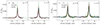 |
Fig. A.1. The normalized fluxes at y = 0 (left panels) and x = 0 (right panels) axis of the Hα-resolved (top row) and UV-resolved (bottom row) clumps selected for the stacking (dashed lines of varying colours) and the corresponding stacked clump (black solid line). The grey shaded area is the 1σ uncertainty of the stacked profile. The axes are normalized for scale quantities as described in Sect. A. |
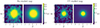 |
Fig. A.2. Maps of the Hα (top panels) and UV (bottom panels) stacked clumps (left panels) and best-fitting models (right panels) obtained with two 2D Moffat (parameters in Table A.1), residuals. The axes and the fluxes are normalized to scale quantities, as described in Sect. A. |
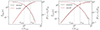 |
Fig. A.3. Comparison between the stacked profile (black lines) and the best-fitting model (red lines) both in the case of Hα (top panel) and UV (bottom panel). The dashed lines show the surface brightness (left y-scale), the solid lines show the cumulative normalized flux (right y-scale). The vertical grey dotted and dash-dotted lines are the core and isophotal radii of the stacked profile. |
In Table A.1 we list the best-fitting values of the morphological parameters of the Moffat functions, already re-normalized where needed. The stacked clumps and the best-fitting models are shown both for Hα and UV in Fig. A.2 as 2D maps. In these maps the axes and the flux  are re-normalized for the average core radius and total flux of the clumps used for the stacking, respectively, while the model flux
  is normalized for the total flux of the best-fitting model. In Fig. A.3, we compare the surface density and the cumulative flux of the stacked clump and the best-fitting model. As one can notice, the profiles are in pretty good agreement within the isophotal radius, which is the constrained interval within which all our clumps were selected and defined, confirming that the models gives good descriptions of the stacked profiles both in the case of Hα and UV. Thanks to this procedure, we retrieved the average intrinsic shape of the a typical Hα or UV clump, that can be re-scaled to physical units according to our purposes.
Appendix B: Modelling the spectral energy distribution
The SED of a clump is comprised of many factors, primarily its age and mass. The former mainly drives the shape of the SED (i.e. the relative flux of the photometric bands with respect to each other). Typical stellar populations younger than 10 Myr and 200 Myr are characterized by strong Hα-line emission and UV continuum, respectively. A clump with age in between 10 and 200 Myr, for example, will still be very bright in the F275W filter, but will have faint or no emission coming from Hα. If the clump is even older than 200 Myr, then, it will get progressively faint in the blue filters of our set. Once the shape of the SED has been determined, it must be scaled to physical units by a factor that depends on the mass-to-light ratio, which is a function of the age of the clump of which we want to create a mock image. The physical fluxes are then used to scale the normalized flux of the stacked clump defined in Sect. A.
In the following sections, we describe the procedures we followed to generate the SED of a mock clump, starting from its shape and then moving to its mass-to-light ratio. As already done to define the intrinsic shape of the clumps (Sect. A), the procedure was followed independently for Hα and UV clumps. Furthermore, in this case we also treated the clumps of different spatial categories (tail, extraplanar, disk) separately.
B.1. Shape of the spectral energy distribution
The aim is to generate a library of normalized SEDs of Hα and UV clumps in different spatial categories as a function of the stellar mass-weighted age. Therefore, for each selection filter and spatial category, we selected all the leaf clumps for which BAGPIPES gives reliable estimates of stellar mass and mass-weighted age (Sect. 2.3), and binned them by age in logarithmic scale (either 4 or 5 bins according to available number of clumps, in order to have enough statistics in each bin). Then the SED of each clump was normalized for the flux in the F814W filter, to make the SEDs of the clumps with different masses comparable. For each age bin and photometric band, a flux distribution was built starting from the clumps normalized fluxes. This choice let us assign to each age bin a median normalized flux with a scatter than can well reproduce the variations in the SEDs even among clumps of similar age. As an example, in Fig. B.1 we show the results of the normalized SEDs for Hα and UV tail clumps. As one can notice, the normalization for the F814W flux forces that filter to be anchored at 1, while the shapes of the SEDs follow pretty well the expected behaviour for the Hα-line emission and the near UV continuum, both getting fainter and fainter with the stellar age.
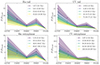 |
Fig. B.1. SED distribution of tail (top row) and extraplanar (bottom row) clumps, normalized for the flux in the F814W filter. Hα clumps are shown in the left panels and UV clumps in the right panels. The clumps are divided in age bins (from purple to yellow). The solid lines are the median SEDs in each age bin, while the shaded area covers the 1σ interval. Details about how these normalized SEDs are obtained are given in Sect. B.1. |
B.1.1. Clump mass-to-light ratios
We define the mass-to-light ratio Mcl/LF814W as the ratio between the clump stellar mass Mcl and the F814W luminosity LF814W. Mcl/LF814W was computed for each age bin by performing a linear fit in the log Mcl − log LF814W plane. The linear fit was performed using the Bayesian fitting tool LINMIX7 (Kelly 2007), including also the intrinsic scatter to the linear relation. As an example, the results concerning tail clumps are shown in Fig. B.2, where the Hα and UV samples are also divided per age bins. As expected, the F814W at a given mass is larger for young clumps (i.e. small Mcl/LF814W). That is, for a given clump mass and age, it is possible to assign the F814W luminosity, which is used to scale the normalized SED defined by its age (Sect. B.1) to physical units.
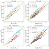 |
Fig. B.2. Clumps log LF814W − log Mcl plane (top row for tail clumps, bottom row for extraplanar clumps, Hα clumps in the left panels, UV clumps in the right panels). The clumps are divided in age bins as described in Sect. B.1 and plotted with different colours and shapes (see the legend). For each age bin, a linear fit to the clumps log LF814W − log Mcl is performed and plotted as solid line of the corresponding bin. |
Appendix C: Radius-mass relation
In order to assign a physical radius to the intrinsic profile obtained in Sect. A for any mock clump of a given mass, we fitted the core radius-mass relation rcore, corr − Mcl with the Bayesian orthogonal linear fitting procedure firstly used in Posti et al. (2018) and described in Bacchini et al. (2019), which let us introduce an intrinsic scatter in the clumps radius at a given mass. The fit was performed only on the clumps which are spatially resolved, defined as the clumps with rcore, corr larger than two full-width half maximum of the HST PSF (Giunchi et al. 2023a). The log-likelihood is the same as in Eq. 6, where Ncl is the number of resolved clumps that are fitted, di is the distance between a given data point  and the model
  . The data points
  were obtained by shifting the physical quantities (log Mcl, log rcore, corr) for their median values to remove the covariance between m and q (which becomes
  after the shift). In this case the total scatter is defined as σtot2 = σ⊥2 + σMi, ⊥2 + σri, ⊥2, where σ⊥ is the orthogonal intrinsic scatter, while σMi, ⊥ = σMi sin θ and σri, ⊥ = σri cos θ are the projections of the
  and
and  uncertainties σMi and σri, respectively (θ = arctanm).
We considered the median of the parameters distributions as the reference parameters and are listed in Table C.1 in the form (m, q, σr), which are the parameters needed to infer the clumps size at a given mass. In Fig. C.1 the size-mass log-plane is shown; we note the good correlations for tail and extraplanar UV clumps (with Pearson’s coefficients larger than 0.5), while the correlations for the Hα clumps are quite weak (especially in the tail, for which the Pearson’s coefficient is 0.29). However, we note that the main purpose of this fitting procedure is to assign a realistic radius to a clump of given stellar mass: in this sense, the presence of a weak correlation is not a problem, since the large scatter is modelled by introducing the intrinsic scatter.
Best-fitting parameters of the radius-mass relation, modelled as described in Sect. C.
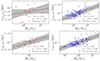 |
Fig. C.1. Core radius-stellar mass relation for tail (top row) and extraplanar (bottom row) resolved clumps (Hα in the left panels and UV in the right panels, respectively). Each clump is plotted as a red (for Hα) or blue (for UV) square with stellar mass uncertainties. The best-fitting linear relation (black solid line) is obtained as described in Sect. C, and the grey area is the 1σ interval of the fit. In the legend, the best-fitting parameters are reported, together with the Pearson coefficient and the P-value. |
Appendix D: Mock clump generation
In the previous sections, we defined all the quantities necessary to generate mock images in all the HST filters for a clump with given mass, age and axial ratio. We generated a set of 1000 Hα clumps and 1000 UV clumps for each galaxy, for which the input parameters listed above were defined as follows:
-
The clump stellar mass Mcl was extracted from a flat distribution ranging from the minimum to the maximum clump stellar mass derived from the real clumps. Thanks to this choice, all masses are uniformly sampled when studying the mass completeness and discrepancy (Sect. 3).
-
The age and axial ratio were extracted from the corresponding distribution of real clumps. In this way, we can explore combinations of mass-age-shape that are realistic and weighted by their frequency in the observed sample. We note that, since the age and axial ratio distributions are taken from observations, they may suffer of incompleteness as well. For a fixed mass, for example, an old clump is fainter in the detection band than a young one. However, a systematic study of the completeness of the age distribution is beyond the scope of this work, it would increase the dimensionality of the problem and would require the study of N2 mock clumps, with N the number of mock clumps studied in this work. Therefore we opted for adopting the observed distribution, in order to be as close as possible to the clump sample, even with no further correction.
Once the intrinsic properties of the clumps were defined, we derived the observables as follows:
-
By means of the size-mass relation, at a given mass we can derive the value of rcore, corr (Sect. C), which was converted to angular scale given the redshift of the galaxy. The intrinsic scatter of the linear relation was taken into account with a Gaussian extraction. The inferred core radius was used to assign a physical angular scale to the clump intrinsic profile (Sect. A), which was then convoluted for the HST PSF.
-
The clump image was stretched for the extracted axial ratio and rotated by a position angle uniformly extracted between 0 and 2π.
-
The shape of the SED of the clump was inferred from the age as follows. As described in Sect. B.1, for each age bin and photometric filter we derived a distribution of normalized fluxes; after uniformly extracting a random number between 0 and 1, we took the normalized flux in each filter at the percentile corresponding to the number extracted. By doing this, we are able to reproduce the variety of SED shapes present in each bin.
-
Given the mass and the age, we derived Mcl/LF814W (Sect. B.1.1) and converted it to F814W flux, which let us scale the normalized SED previously determined to a physical quantity. Given the fluxes in the 5 photometric filters, we generated an image of the clump for each filter, by multiplying the clump intrinsic profile for the corresponding flux.
-
The clump images of each filter were convoluted for the corresponding PSF curve.
That is, we created a library of 1000 mock Hα clumps (and 1000 mock UV) for each galaxy, each of which constituted by 5 images. As examples, we show in Fig. D.1 three F275W mock images of UV mock clumps generated to belong to JO201. The clumps have masses 5 × 10⁴ M⊙, 5 × 10⁵ M⊙ and 5 × 10⁶ M⊙. We note the increasing scale of the image, due to the increasing mass and size of the mock clumps, and the variety of elongations and position angles.
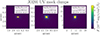 |
Fig. D.1. Examples of F275W mock images of three UV clumps generated for JO201 as described in Sect. D. The red ellipse is built using the semi-major axis, semi-minor axis and position angle of the clump. For each clump, the stellar mass, core radius, axis ratio and position angle are reported in the legend. |
Appendix E: Re-detection of the mock clumps
The aim of these mock observations is to quantify the effects of background noise and contamination by background and foreground sources on the detection of clumps in the tails of the jellyfish galaxies of our sample. The classical way to mimic the same conditions affecting the galaxy real images consists of adding the mock clumps images to the real images themselves, perform the same procedure adopted to detect the real clumps and check whether mock clumps are re-detected and what their output properties are. The way the mock clumps were added to the image was different whether we were studying tail or extraplanar clumps and it was based on the need not to change the crowding properties of the corresponding region of the studied galaxy. The two methods are listed below.
Mock clumps addition in the tails. In order to evenly cover the area of the image where the clump detection was run, the field of view of each galaxy was divided in a grid of Ncell squared cells (700 pixels in size for JO175, JO206 and JW100, 800 for JO201, JO204, JW39). Then a number of mock clumps equal to the number of cells was randomly extracted by the corresponding library (Sect. D) and added to each cell. The centre of the clump was randomly extracted within a square region of size 350/400 pixels (half of the cell size), centred in the corresponding cell. This was done in order to fully explore the background conditions inside a certain cell, still avoiding to place the mock clump at the border of the cell and therefore to overlap it with other adjacent mock clumps. Furthermore, the centre of the mock clump could not be inside the galactic optical disk. For the subsequent mock observation, the cell grid was shifted both along RA and Dec by 350/400 pixels, again to exhaustively explore the whole galactic FOV. As examples, in Fig. E.1 we show the first two mock observations for JO201, where one can notice where the mock clumps are added, how the FOV is divided in cells and how the grid is shifted in the second mock observation. In order to have a statistically robust estimate of the completeness and input-output discrepancy in the whole mass interval, we studied at least 1000 mock clumps per galaxy, which results in Nmock = 1000/Ncell mock observations (rounded up).
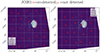 |
Fig. E.1. First two F275W mock images generated for JO201 following the prescription in Sect. E. The white dotted lines define the grid in which the FOV is divided, while the white shaded area is the optical disk (Sect. 2.1). The mock clumps that are added to the real images are inside a red circle if they got re-detected, otherwise they are marked by a red cross. |
Mock clumps addition in the extraplanar region. The extraplanar region is located in the outskirts of the galactic stellar disk (as described in Sect. 2.1). Being this region highly irregular in all the six galaxies of the sample, we could not apply the same aforementioned procedure used for the tail clumps. That is, we opted for a random extraction of the position of the clumps within the extraplanar area. The number of added mock clumps per iteration in a given galaxy was chosen to be equal to the Poissonian uncertainty on the number of real extraplanar clumps detected in that galaxy Nextra, g, which is  . This choice allows us to add clumps without changing the crowding conditions of the real sample of clumps. The total number of simulated mock clumps is about 104 in Hα and 1.4 × 10⁴ in UV.
Once the mock image is ready, we re-ran the clumps detection (Sect. 2.2). From now on, we call this catalogue the new catalogue, while the one with real clumps is the original catalogue. The new catalogue was matched with the original one to find re-detected real clumps: if the centre of an original clump was within a circle centred in the centre of a new clump and radius equal to the new clump core radius (Giunchi et al. 2023a), and their fluxes were comparable within a factor of 2, then the new clump was flagged as a re-detected original clump and removed by the new catalogue. The remaining new clumps were matched with the mock clumps that were added to the image, and if the centre of a mock clump was within the area of a new clump, the new clump was flagged as a re-detected mock clump. Mock clumps not matched to any new clump were flagged as non-detected. Finally, the mass and mass-weighted age of the re-detected mock clumps were derived with BAGPIPES in the same way described in Sect. 2.3. After having followed these steps, out of 6125 Hα and 6125 UV clumps, we re-detected and computed stellar masses for 3416 and 2982, respectively. To summarize, at the end of this process we could study the fraction of lost mock clumps as a function of their input mass while, for those that are re-detected, we could compare the input mass with the one resulting from BAGPIPES.
Appendix F: Completeness and mass estimation bias
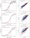 |
Fig. F.1. Plots of the completeness (left column) and mass estimation bias (right column), as in Fig. 3, but for UV tail (top row), Hα extraplanar (middle row) and UV extraplanar (bottom row) clumps. The parameters are estimated as in Sects. 3.1 and 3.2, listed in Table 2 and the plots shown in Fig. F.1. |
Appendix G: Testing the mass function fitting method
In order to test the reliability of the fitting method, we generated two samples of mock clumps from a distribution of equation

where MF is the intrinsic mass function and C is the completeness function (3.1), for which we assumed the same parameters derived for the tail Hα clumps. We tested two different functional forms for the mass function, which are the most used and debated in literature to fit observations: sample A was extracted from a power-law mass function MF ∝ M*−α, with slope α = 2; sample B was extracted from a Schechter function MF ∝ M*−α e−M*/Mc, with slope α = 2 and cut-off mass log Mc = 105.5 M⊙.
In testing the likelihood of Eq. 7, we fitted both samples either assuming a power-law function or a Schechter mass function and varying the sample size from ∼1000 to ∼100 clumps (with the latter case resembling our typical conditions). The aim is to understand if the slope can be correctly retrieved and how the presence of the cut-off affects our results. Applying a certain mass function to one of the two samples brings to the following results, as a function of the sample size:
-
Fitting sample A with a power law, first two panels of Fig. G.1: the fitting procedure correctly retrieves the input slope within 1σ, with the sample size affecting just the uncertainty on the estimate.
-
Fitting sample A with a Schechter, top row of Fig. G.2: regardless of the sample size, the retrieved cut-off mass is larger than the most massive clump of the sample, correctly indicating that an exponential cut-off is absent within the fitted range of masses. For what concerns the slope, the value inferred by the model underestimates the intrinsic one (yet being consistent within 3σ), with the sample size affecting just the uncertainties.
-
Fitting sample B with a power law, last two panels of Fig. G.1: as shown and discussed in previous works (Gieles 2009), the presence of a cut-off leads to a slope steeper than the input one, since it is not taken into account by the chosen functional form chosen to fit the mass function. This happens regardless of the sample size, which affects the uncertainties.
-
Fitting sample B with a Schechter, bottom row of Fig. G.2: in this case the sample size highly affects the results. With a large available statistics (left panel), the fitting procedure correctly infers both the input slope and cut-off mass. When the sample is small (right panel), the cut-off mass is still well constrained, while the slope is not constrained and only an upper limit on it can be put.
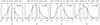 |
Fig. G.1. Histogram of the best-fitting slope α distribution, obtained fitting a power-law mass function to a sample of mock clumps extracted either from a power-law function (first two panels) or a Schechter function (last two panels). The plots to the left refer to cases in which the fitted sample was large (∼1000 objects), while for those to the right the sample was small (∼100 objects). When present (because within the interval of explored values), the red line marks the input slope assumed for both the power-law and the Schechter mock distributions (α = 2). The values in the legend of each histogram are the median of each distribution for the corresponding parameter, with uncertainties given by the 84th percentile minus the median and the median minus the 16th percentile (upper and lower uncertainty, respectively). The same values are also reported as black dashed vertical lines in the histograms. |
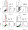 |
Fig. G.2. Corner plots of the parameter space (α, log Mc) (the slope and the cut-off mass, respectively), obtained fitting a Schechter mass function to a sample of mock clumps extracted either from a power-law (top row) or a Schechter (bottom row) function. The plots to the left refer to cases in which the fitted sample was large (∼1000 objects), while for those to the right the sample was small (∼100 objects). The red line marks the input slope of both the power-law and the Schechter mock distributions (α = 2). The green line marks the cut-off mass (log Mc/M⊙), which is present only in the case of the Schechter. Values on top of each histogram are the median of each distribution for the corresponding parameter, with uncertainties given by the 84th percentile minus the median and the median minus the 16th percentile (upper and lower uncertainty, respectively). The same values are also reported as black dashed vertical lines in the histograms. |
These tests suggest that fitting a Schechter function puts good constraints about the presence of the exponential cut-off (and therefore if the shape of the mass function is a power law of a Schechter function), independently on the size of the sample. However, when the available statistics is small (about 100 objects), the slope can not be constrained, especially if the intrinsic shape of the mass function is a Schechter function. Typically, fitting a power law gives steeper values for the slope than the intrinsic one, if the real shape of the mass function is a Schechter, but can be the only method to put constraints on this parameter.
All Tables
Best-fitting parameters of the completeness and mass bias functions for the Hα tail (first row), Hα extraplanar (second row), UV tail (third row), and UV extraplanar (fourth row) mock clumps.
Best-fitting parameters of the two 2D Moffat functions used to model the stacked clumps.
Best-fitting parameters of the radius-mass relation, modelled as described in Sect. C.
All Figures
|
Fig. 1. RGB images of the six studied galaxies. The galaxies are JO201 and JO206 (top row), JW100 and JO204 (middle row), JW39 and JO175 (bottom row). The images are obtained following the prescription given in Gullieuszik et al. (2023) and summarized in Sect. 2. The white and black contours separate the tail, extraplanar, and disk regions, as described in Sect. 2.1. The white shaded area highlights the disk region, which is not considered throughout this work. The two contours almost coincide in JW39 and JO175 (bottom left and bottom right panels, respectively). The blue squares and red dots mark the position of UV and Hα leaf clumps with robust mass estimates (Giunchi et al. 2023a; Werle et al. 2024), summarized in Sects. 2.2 and 2.3. The pink arrow points towards the centre of the galaxy cluster (taken from Cava et al. 2009 and Biviano et al. 2017). |
| In the text | |
|
Fig. 2. Stellar mass (top row) and mass-weighted age (bottom row) distributions of Hα (red histograms) and UV (blue histograms) clumps. The clumps were divided into tail (left panels) and extraplanar (right panels) according to the criteria described in Sect. 2.1, and the sample was selected following the procedure described in Sect. 2.3. |
| In the text | |
|
Fig. 3. Completeness (left) and mass estimation bias (right) for Hα tail clumps. In the left panel the red solid line is the best-fitting model computed as in Eq. (4), cut to 0 for values below 0.5 (Sect. 3.1), while the red dashed line shows the uncut function. The threshold value of 0.5, below which the function is forced to 0, is plotted as a grey dotted line. The black empty circles show the binned mass completeness derived from the mock clumps (with uncertainties equal to the Poissonian error), for a qualitative visualization of the goodness of the fit (the fitting technique does not depend on the binning). The right panel shows the relationship between the observed (x-axis) and intrinsic (y-axis) mass for the Hα tail re-detected mock clumps. Each clump is plotted as a blue dot. The black dashed line is the 1:1 relation. The red contours are computed from the best-fitting model describing the clumps distribution (Eq. (5)). |
| In the text | |
|
Fig. 4. Posterior distribution of the slope parameters α, inferred fitting a power law to the mass distribution of tail clumps (first two panels) and extraplanar clumps (last two panels). Hα is on the left, and UV is on the right. The vertical dashed black lines are the 16th, 50th, and 84th percentiles, also reported in the legends. |
| In the text | |
|
Fig. 5. Corner plots of the parameter space (α, log Mc) (the slope and the cut-off mass, respectively), obtained fitting a Schechter mass function (Eq. (8)) to the Hα and UV tail (top row) and extraplanar (bottom row) clump mass distribution. The values at the top of the histograms are the median of each distribution for the corresponding parameter, with uncertainties given by the 84th percentile minus the median and the median minus the 16th percentile (upper and lower uncertainty, respectively). The same values are also reported as black dashed vertical lines in the histograms. |
| In the text | |
|
Fig. A.1. The normalized fluxes at y = 0 (left panels) and x = 0 (right panels) axis of the Hα-resolved (top row) and UV-resolved (bottom row) clumps selected for the stacking (dashed lines of varying colours) and the corresponding stacked clump (black solid line). The grey shaded area is the 1σ uncertainty of the stacked profile. The axes are normalized for scale quantities as described in Sect. A. |
| In the text | |
|
Fig. A.2. Maps of the Hα (top panels) and UV (bottom panels) stacked clumps (left panels) and best-fitting models (right panels) obtained with two 2D Moffat (parameters in Table A.1), residuals. The axes and the fluxes are normalized to scale quantities, as described in Sect. A. |
| In the text | |
|
Fig. A.3. Comparison between the stacked profile (black lines) and the best-fitting model (red lines) both in the case of Hα (top panel) and UV (bottom panel). The dashed lines show the surface brightness (left y-scale), the solid lines show the cumulative normalized flux (right y-scale). The vertical grey dotted and dash-dotted lines are the core and isophotal radii of the stacked profile. |
| In the text | |
|
Fig. B.1. SED distribution of tail (top row) and extraplanar (bottom row) clumps, normalized for the flux in the F814W filter. Hα clumps are shown in the left panels and UV clumps in the right panels. The clumps are divided in age bins (from purple to yellow). The solid lines are the median SEDs in each age bin, while the shaded area covers the 1σ interval. Details about how these normalized SEDs are obtained are given in Sect. B.1. |
| In the text | |
|
Fig. B.2. Clumps log LF814W − log Mcl plane (top row for tail clumps, bottom row for extraplanar clumps, Hα clumps in the left panels, UV clumps in the right panels). The clumps are divided in age bins as described in Sect. B.1 and plotted with different colours and shapes (see the legend). For each age bin, a linear fit to the clumps log LF814W − log Mcl is performed and plotted as solid line of the corresponding bin. |
| In the text | |
|
Fig. C.1. Core radius-stellar mass relation for tail (top row) and extraplanar (bottom row) resolved clumps (Hα in the left panels and UV in the right panels, respectively). Each clump is plotted as a red (for Hα) or blue (for UV) square with stellar mass uncertainties. The best-fitting linear relation (black solid line) is obtained as described in Sect. C, and the grey area is the 1σ interval of the fit. In the legend, the best-fitting parameters are reported, together with the Pearson coefficient and the P-value. |
| In the text | |
|
Fig. D.1. Examples of F275W mock images of three UV clumps generated for JO201 as described in Sect. D. The red ellipse is built using the semi-major axis, semi-minor axis and position angle of the clump. For each clump, the stellar mass, core radius, axis ratio and position angle are reported in the legend. |
| In the text | |
|
Fig. E.1. First two F275W mock images generated for JO201 following the prescription in Sect. E. The white dotted lines define the grid in which the FOV is divided, while the white shaded area is the optical disk (Sect. 2.1). The mock clumps that are added to the real images are inside a red circle if they got re-detected, otherwise they are marked by a red cross. |
| In the text | |
|
Fig. F.1. Plots of the completeness (left column) and mass estimation bias (right column), as in Fig. 3, but for UV tail (top row), Hα extraplanar (middle row) and UV extraplanar (bottom row) clumps. The parameters are estimated as in Sects. 3.1 and 3.2, listed in Table 2 and the plots shown in Fig. F.1. |
| In the text | |
|
Fig. G.1. Histogram of the best-fitting slope α distribution, obtained fitting a power-law mass function to a sample of mock clumps extracted either from a power-law function (first two panels) or a Schechter function (last two panels). The plots to the left refer to cases in which the fitted sample was large (∼1000 objects), while for those to the right the sample was small (∼100 objects). When present (because within the interval of explored values), the red line marks the input slope assumed for both the power-law and the Schechter mock distributions (α = 2). The values in the legend of each histogram are the median of each distribution for the corresponding parameter, with uncertainties given by the 84th percentile minus the median and the median minus the 16th percentile (upper and lower uncertainty, respectively). The same values are also reported as black dashed vertical lines in the histograms. |
| In the text | |
|
Fig. G.2. Corner plots of the parameter space (α, log Mc) (the slope and the cut-off mass, respectively), obtained fitting a Schechter mass function to a sample of mock clumps extracted either from a power-law (top row) or a Schechter (bottom row) function. The plots to the left refer to cases in which the fitted sample was large (∼1000 objects), while for those to the right the sample was small (∼100 objects). The red line marks the input slope of both the power-law and the Schechter mock distributions (α = 2). The green line marks the cut-off mass (log Mc/M⊙), which is present only in the case of the Schechter. Values on top of each histogram are the median of each distribution for the corresponding parameter, with uncertainties given by the 84th percentile minus the median and the median minus the 16th percentile (upper and lower uncertainty, respectively). The same values are also reported as black dashed vertical lines in the histograms. |
| In the text | |
Current usage metrics show cumulative count of Article Views (full-text article views including HTML views, PDF and ePub downloads, according to the available data) and Abstracts Views on Vision4Press platform.
Data correspond to usage on the plateform after 2015. The current usage metrics is available 48-96 hours after online publication and is updated daily on week days.
Initial download of the metrics may take a while.