| Issue |
A&A
Volume 696, April 2025
|
|
|---|---|---|
| Article Number | A72 | |
| Number of page(s) | 15 | |
| Section | Stellar structure and evolution | |
| DOI | https://doi.org/10.1051/0004-6361/202451565 | |
| Published online | 04 April 2025 | |
Evolution of stars with 60 and 200 M⊙: predictions for WNh stars in the Milky Way
1
Nicolaus Copernicus Astronomical Center, Polish Academy of Sciences, Bartycka 18, 00-716 Warsaw, Poland
2
Astronomický ústav, Akademie věd Ceské republiky, Fričova 298, 251 65 Ondřejov, Czech Republic
3
Department of Astronomy and Astrophysics, University of California San Diego, La Jolla, California 92093, USA
⋆ Corresponding author; This email address is being protected from spambots. You need JavaScript enabled to view it.
Received:
18
July
2024
Accepted:
3
March
2025
Abstract
Context. Massive stars are characterised by powerful stellar winds driven by radiation; thus, the mass-loss rate is known to play a crucial role in their evolution.
Aims. We study the evolution of two massive stars (a classical massive star and a very massive star) at solar metallicity (Z = 0.014) in detail. We calculate their final masses, radial expansion, and chemical enrichment, at their H-core, He-core, and C-core burning stages, prior to their final collapse.
Methods. We ran evolutionary models for initial masses of 60 and 200 M⊙ using MESA and the Geneva-evolution-code (GENEC). For the mass loss, we adopted the self-consistent m-CAK prescription for the optically thin winds of OB-type stars, a semi-empirical formula for H-rich optically thick wind of luminous Wolf-Rayet (WR) stars of the nitrogen sequence with hydrogen in their spectra (WNh stars), and a hydrodynamically consistent formula for the H-poor thick wind of classical WR stars. The transition from thin to thick winds was set to Γe = 0.5.
Results. The unification of the initial set-up for the stellar structure and wind prescription leads to very similar black hole mass for both GENEC and MESA codes, but both codes predict different tracks across the Hertzsprung-Russell diagram (HRD) For the 60 M⊙ case, the GENEC model predicts a more efficient rotational mixing and more chemically homogeneous evolution, whereas the MESA model predicts a large radial expansion that reaches the Luminous Blue Variable (LBV) phase. For the 200 M⊙ case, differences between both evolution codes are less relevant because their evolution is dominated by wind mass loss with a weaker dependence on internal mixing.
Conclusions. The switch of the mass-loss prescription based on the Eddington factor instead of the removal of outer layers, implies the existence of WNh stars with a large mass fraction of hydrogen at the surface (Xsurf ≥ 0.3) formed from initial masses of ≳60 M⊙. These stars are constrained in a Teff range of the HRD which corresponds to the main sequence band, in agreement with the observations of Galactic WNh stars at Z = 0.014. While our models employ a fixed Γe, trans threshold for the switch to thick winds, rather than a continuous thin-to-thick wind model, the good reproduction of observations during the main sequence supports the robustness of the wind model upgrades, allowing its application to studies of late-stage stellar evolution before core collapse.
Key words: stars: early-type / stars: evolution / stars: massive / stars: mass-loss / stars: winds / outflows / stars: Wolf-Rayet
Deceased on 13th January 2024.
© The Authors 2025
 Open Access article, published by EDP Sciences, under the terms of the Creative Commons Attribution License (https://creativecommons.org/licenses/by/4.0), which permits unrestricted use, distribution, and reproduction in any medium, provided the original work is properly cited.
This article is published in open access under the Subscribe to Open model. This email address is being protected from spambots. You need JavaScript enabled to view it. to support open access publication.
1. Introduction
The detection of the first source of gravitational waves (GW, Abbott et al. 2016, 2021) opened the door to a large number of studies dedicated to find more GW sources in the Universe, in particular, double compact object (hereafter DCO) mergers. The rates of these DCO merger events depend on the considered conditions for the binary system with respect to the orbital separation and the formation (or otherwise) of a common envelope (CE), as well as the initial assumptions for RLOF and their timescales (Ivanova et al. 2013; Olejak et al. 2021). Moreover, these modes are intimately linked with the single evolution of the stars in a binary system, which is crucial to determine the final remnant masses (Yungelson et al. 2008; Belczynski et al. 2010; Yusof et al. 2013; Spera & Mapelli 2017; Bavera et al. 2023; Martinet et al. 2023) and the maximum radial expansion that the stellar components can reach during their evolution (Agrawal et al. 2020; Romagnolo et al. 2023). Thus, accurate evolution models are necessary to constrain the theoretical rate of DCO merging events.
Stellar black holes are the final fate of massive stars, with Mzams ≳ 25 M⊙ (Heger et al. 2003). Even though the conditions of stellar death as supernovae also constrain the mass of the final remnant (Fryer et al. 2022; Olejak et al. 2022), the stellar mass prior to the supernova explosion is explicitly dependent of the mass-loss rate (denoted as dM/dt or simply Ṁ) enacted by the strong winds during the evolution of a massive stars (Vink 2022). Because stellar winds of hot massive stars are driven by the line force (Lucy & Solomon 1970; Castor et al. 1975; Abbott 1982), these Ṁ values are directly dependent on metallicity. This explains the predominance of more massive black holes in less metallic environments (Farrell et al. 2021; Vink et al. 2021), although exceptions due to unusually weaker winds can also be theoretically described (Belczynski et al. 2020a). Moreover, the strength of the stellar winds varies along the evolution of the star, which is dominated during the main sequence (H-core burning stage) by line-driven optically thin winds for OB-type stars (Puls et al. 2008), then eventual strong outflows might originate during the Luminous Blue Variable (LBV) stage (Humphreys et al. 2016). Finally, we find optically thick winds of Wolf-Rayet (WR) stars for the more evolved stages (Crowther 2007; Gräfener & Hamann 2008). Optically thick winds are naturally denser and, therefore, the mass loss during the WR phase is higher in comparison with the OB-type phase.
Recent theoretical (Krtička & Kubát 2017, 2018; Gormaz-Matamala et al. 2019, 2022a; Björklund et al. 2021) and empirical studies (Hawcroft et al. 2021, 2024) have found theoretical values for the Ṁ of massive stars to be about three times lower than the standard mass-loss recipe from Vink et al. (2001, hereafter V01). Such a difference in the value of mass loss is enough to alter the evolution of stars with Mzams ≳ 20 M⊙ (Meynet et al. 1994). In adopting new winds, massive stars will retain more mass during their main sequence phase, thus they would be bigger and more luminous (Gormaz-Matamala et al. 2022b; Björklund et al. 2023). In addition, massive stars keep larger rotational velocities for a more extended time because they lose less angular momentum (Gormaz-Matamala et al. 2023). Even though these changes in the stellar evolution have been applied mostly for the early H-burning stages, they also impact the further evolution of the subsequent stages (Gormaz-Matamala et al. 2024; Josiek et al. 2024). Moreover, considering that also the mass-loss prescription for WR winds has been revisited (Bestenlehner 2020; Sander & Vink 2020) as well as its impact on stellar evolution (Higgins et al. 2021), the entire panorama of the stellar evolution is being upgraded.
In Romagnolo et al. (2024, hereafter Paper I), we calculated the remnant mass for a set of initial masses from 10 to 300 M⊙ for Z = 0.014, based on stellar evolution models adopting the state-of-the-art physical ingredients, such as a Tayler-Spruit dynamo, greater core-convective overshooting, and new mass-loss recipes. As a result, we found a maximum black hole mass of Mbh, max = 28.3 M⊙ formed from stars with Mzams ≳ 250 M⊙. This is larger than the previous Mbh, max ≃ 20 M⊙ from Belczynski et al. (2010) but quite below the maximum BH masses predicted by Bavera et al. (2023, ≃35 M⊙ at Mzams = 75 M⊙) and Martinet et al. (2023, ≃42 M⊙ at Mzams = 180 M⊙). Even though the recently discovered largest BH in the Milky Way has a mass of Mbh, max = 32.7 ± 0.70 M⊙ (Gaia Collaboration 2024), the low metallicity of its star companion suggest that this black hole was formed from a massive, metal-poor star and, thus, our predicted Mbh, max remains valid.
Moreover, the new wind prescription introduced in Paper I introduces further implications concerning the evolution of massive stars. Standard evolution models (Ekström et al. 2012; Choi et al. 2016) adopted the switch from OB-type to WR-type winds once the stellar surface removes the majority of its hydrogen. Nevertheless, theoretical studies have found that the transition from optically thin to thick winds during the evolution of massive stars is attributed more to the proximity to the Eddington limit, rather than the removal of the outer envelopes (Vink et al. 2011; Gräfener et al. 2011), thus altering the expected lifetimes and total amount of mass removed at each evolutionary stage. Therefore, in Paper I, we set the switch between optically thin to optically thick winds according to the proximity to the Eddington limit, instead of based on the chemical composition of the stellar outer envelope. As a consequence, the most massive stars already develop thick winds during their earliest evolution stages, altering their tracks over the HR diagram and predicting the existence of WR stars with hydrogen abundance Xsurf ≥ 0.3 on their surfaces, which have since been dubbed WNh stars (Martins et al. 2008; Crowther et al. 2010).
In this work, we study in detail the impact of the already mentioned upgrades on the evolution of two stars from Paper I, with a special emphasis on the existence of H-rich WR stars. For that purpose, we run evolution models for the stars with initial masses of 60 and 200 M⊙ at solar metallicity (Z = 0.014), following Asplund et al. (2009). We introduce our mass-loss prescription in Sect. 2, together with the description of the switch from optically thin to thick winds at Γe = 0.5. The resulting evolution tracks over the HR diagram for our models are detailed in Sect. 3, whereas the observational diagnostics comparing with spectroscopic analyses are shown in Sect. 4. Finally, our conclusions are summarised in Sect. 5.
2. Ingredients for stellar evolution models
2.1. Stellar evolution codes
As in Paper I, we perform our stellar evolution models using the codes Modules for Experiments in Stellar Astrophysics (Paxton et al. 2011, 2013, 2015, 2018, 2019; Jermyn et al. 2023, MESA) and the Geneva-evolution-code (Eggenberger et al. 2008, hereafter GENEC). For step-overshooting, we adopted a value for αov of 0.5, in agreement with the most recent studies on convective cores (Martinet et al. 2021; Scott et al. 2021; Baraffe et al. 2023). Concerning the angular momentum transport, we included the Tayler-Spruit dynamo for both MESA and GENEC codes (Tayler 1973; Spruit 2002; Heger et al. 2005), whereas we replaced the treatment for the convective layers from Schwarzchild to Ledoux’s criterion (Ledoux 1947). For the convective outer layers, MESA adopts a mixing-length parameter of αMLT = 1.82, whereas GENEC keeps αMLT = 1.6. In order to reduce the superadibaticity in regions near the Eddington limit, we used the use_superad_reduction method, which is said to be a more constrained and calibrated prescription than MLT++ in MESA (Jermyn et al. 2023). In particular, this difference in the superadiabacity treatment will be relevant during the VMS evolution across the He-core burning stage (Romagnolo et al. 2025), as we observe in Sect. 3.2.
2.2. Mass loss for massive and very massive stars
The evolutionary tracks of massive stars adopting lower Ṁ values are in line with the observed mass loss of clumped winds (Bouret et al. 2005; Muijres et al. 2011; Šurlan et al. 2013) and with more detailed calculations for the wind structure of O-type stars thanks to the self-consistent solution of the radiative transfer equations at full NLTE conditions (Sander et al. 2017; Sundqvist et al. 2019; Gormaz-Matamala et al. 2021). However, this scenario can hardly be extended to higher masses such as VMS, whose mass-loss rates values even larger than the given ones by V01 (Vink et al. 2011). Their stellar winds are so strong that they develop WR-type spectral profile with broad emission lines before the end of the H-core burning stage (WNh stars). The limit between VMS and ‘regular’ massive stars is typically set around Mzams ∼ 100 M⊙, although this value may vary by means of rotation, metallicity, and especially mass-loss input (Yusof et al. 2013; Köhler et al. 2015).
The evolution of VMS, revisiting the transition between formal O-type to WNh stars, was recently analysed by Gräfener (2021) and Sabhahit et al. (2023). Nonetheless, standard evolution codes still assume the transition of the wind regime based on the surface composition (when the hydrogen mass fraction becomes Xsurf ≤ 0.3 for GENEC and Xsurf ≤ 0.4 for MESA). Also, the mass-loss recipe switches from the prescription for optically thin V01 to optically thick winds according to Gräfener & Hamann (2008, hereafter GH081) in GENEC, whereas MESA uses the prescription of Nugis & Lamers (2002) for WR winds. However, spectroscopic diagnostics have found WNh spectral features for VMS with surface hydrogen abundances as high as Xsurf ≃ 0.7 in the Milky Way (Martins 2023) and in the Large Magellanic Cloud (Tehrani et al. 2019; Martins & Palacios 2022), thus strengthening the idea that the transition to thick winds should be based on another criteria apart from surface chemical composition.
2.3. Winds in the proximity to the Eddington limit
The mass loss of VMS is directly dependent on the Eddington factor and the relationship quickly escalates when the Eddington limit is approached (Vink et al. 2011; Vink & Gräfener 2012). The Eddington limit defines the limit for the hydrostatic stability of a star and it corresponds when the outwards radiative force equals to the inwards gravitational force2 (Langer 1997). This limit is better illustrated by the “classical” Eddington factor, which considers only the electron scattering for the radiative processes,
 (1)
(1)
with κe being the electron scattering opacity. Assuming a fully ionised plasma, the Eddington factor is usually expressed as a function of stellar mass, luminosity, and hydrogen abundance
 (2)
(2)
namely, the classical Eddington factor depends only on the fundamental stellar parameters.
Numerical models found a kink in the slope of the Ṁ ∝ Γe dependence at Γe ≃ 0.7, after which the mass-loss scales with the Eddington factor in agreement with the relationship found for Gräfener & Hamann (2008) for late-type WN stars (WNL). Indeed, Γe = 0.7 was already used as a transition criterion to switch from O-type to WR stars in evolution models (Chen et al. 2015). Posteriori observational diagnostics on very massive stars found that wind clumping and uncertainties affects the accuracy to determine the kink in the Γe space, which can be set as low as Γe ≃ 0.3 (Bestenlehner et al. 2014), even though this value for the Eddington factor strongly depends on the mass estimations derived from the L/M relations from Gräfener et al. (2011). A more theoretically detailed study is provided by Sabhahit et al. (2023), where the switch on the wind regime is directly correlated with the wind efficiency η = Ṁv∞/(L/c) at different metallicities. In this case, the mass loss of the initial O-type phase is described by the V01, rather than more recent recipes (e.g. Krtička & Kubát 2017; Björklund et al. 2021; Gormaz-Matamala et al. 2022b).
Instead, we aim for a transition point between thin and thick winds, independent not only of the initial mass-loss rate adopted but also independent on the wind momentum. For this purpose, we based our transition in the upper limit of validity of our m-CAK prescription (Gormaz-Matamala et al. 2022a), where both Ṁ and the wind velocity profile v(r) are self-consistently calculated together with the line-force parameters (Gormaz-Matamala et al. 2019). Bestenlehner (2020) extended the theoretical calculation of Ṁ according to the CAK theory (Castor et al. 1975) for regimes closer to the Eddington limit, also finding a transition Γe, trans beyond the which the slope of the relation Ṁ ∝ Γe become steeper, in line with the observations of WNh stars exhibiting thick winds from Bestenlehner et al. (2014). This Γe, trans ranges from ∼0.46 to ∼0.48, depending on the value of the CAK line-force parameter3α. For α ∼ 0.4 − 0.6, which are the values found from the self-consistent line-force parameters found by Gormaz-Matamala et al. (2022b) for stars with masses in the range of 25–120 M⊙ and metallicities from Z = 0.014 (solar) to = 0.002 (SMC), the value of the transition Eddington factor keeps relatively constant around Γe, trans ≃ 0.48. Therefore, given that our new prescription for optically thin winds is based on the m-CAK theory, we established Γe = 0.5 as the transition point between thin and thick winds for our evolution models. The thickness in this case means the dominance of the electron scattering on the radiative acceleration, above the line-driven contribution. We discuss the physical implications of this transition in Section 4.1.
2.4. Mass-loss recipes for thin and thick winds
2.4.1. Mass loss for the H-core burning stage
For thin winds (Γe ≤ 0.5), we use the mass-loss prescription from Gormaz-Matamala et al. (2022b); Gormaz-Matamala et al. (2023) as follows:
![Mathematical equation: $$ \begin{aligned} \log \dot{M}_{\rm thin}&=-40.314 + 15.438\,w + 45.838\,x - 8.284\,w\,x \nonumber \\&\quad + 1.0564\,y - w\,y / 2.36 - 1.1967\,x\,y\nonumber \\&\quad +z\times \left[0.4+\frac{15.75}{M_*/M_\odot }\right], \end{aligned} $$](/articles/aa/full_html/2025/04/aa51565-24/aa51565-24-eq3.gif) (3)
(3)
where Ṁthin is in M⊙ yr−1; and where w, x, y, and z are defined as
 (4)
(4)
As mentioned in Gormaz-Matamala et al. (2023), the dependence between mass loss and metallicity is not constant but it intrinsically depends on the mass (and the luminosity) because the radiative acceleration for more massive and luminous stars is mostly dominated by the continuum over the line-acceleration (see also Krtička & Kubát 2018).
The range of validity of Eq. (3) is for Teff ≥ 30 kK and log g ≥ 3.2. Beyond these values, we return to V01 by default, even though the Ṁ for stars in the range of 10 − 30 kK needs to be eventually also decreased (de Burgos et al. 2024). For cases where Teff ≤ 10 kK, the mass loss is described by de Jager et al. (1988).
For thick winds (Γe > 0.5), since we have established the transition based on the theoretical analysis of Bestenlehner (2020), we can use their Ṁ(Γe) recipe with the calibration performed by Brands et al. (2022) as follows:
 (5)
(5)
It is easy to see that for Γe = 0.5, Eq. (4) becomes log Ṁ ≃ −5.04. This value is very close to the ‘transition’ mass-loss rates empirically determined for the Arches cluster by Vink & Gräfener (2012) and for 30 Dor by Sabhahit et al. (2023), namely, the value for Ṁ over the which the stars of the mentioned clusters exhibit a WNh spectrum. This implies that both approaches (i.e. that of Sabhahit et al. 2023, and this current study) find the transition mass-loss rate between thin and thick winds to be roughly the same value. Moreover, because this formula was calibrated for the VMS in the R136 star cluster at the LMC, with metallicity Z = 0.006 (Eggenberger et al. 2021), we added an extra term with the same metallicity dependence as for thin winds. Thus, we have
![Mathematical equation: $$ \begin{aligned} \log \dot{M}_{\rm thick}=\log \dot{M}_{\rm B22}+\log \left(\frac{Z_*}{Z_{\rm LMC}}\right)\times \left[0.4+\frac{15.75}{M_*/M_\odot }\right]. \end{aligned} $$](/articles/aa/full_html/2025/04/aa51565-24/aa51565-24-eq6.gif) (6)
(6)
Despite the fact that we are using the same Γe, trans for all metallicities, the mass loss for optically thick winds incorporates a metallicity dependence, which is consistent with the intrinsic dependence on mass and luminosity. Even though the calibration from Brands et al. (2022) matches with the formula of Krtička & Kubát (2018) (and subsequently with their intrinsic metallicity dependence on luminosity), we adopted the intrinsic metallicity dependence on mass introduced by Gormaz-Matamala et al. (2023) to maintain coherence between our adopted thin and thick winds.
Analogously to Eq. (3) for thin winds, Eq. (5) is valid only for Teff ≥ 30 kK. For thick winds at cooler temperatures, we return to V01; thus their predicted bi-stability jump is still being implemented for all the temperature range between 10 and 30 kK for both Ṁthin and Ṁthick.
2.4.2. Mass loss for advanced evolutionary stages
The expression in Eq. (5) from Bestenlehner (2020) and Brands et al. (2022) is valid for H-rich WR stars for both the H-core or the He-core burning stages. Once the star has depleted the most part of its hydrogen (Xsurf ≤ 10−7), the mass-loss rate follows the formula derived from the hydrodynamically consistent models for WR stars from Sander et al. (2020), whose final formula Ṁ ∼ Γe is given by Sander & Vink (2020)
![Mathematical equation: $$ \begin{aligned} \log \dot{M}=a\log [-\log (1-\Gamma _{\rm e})]-\log 2\left(\frac{\Gamma _{\rm e,d}}{\Gamma _{\rm e}}\right)^{c_{d,b}}+\log \dot{M}_{\rm off}, \end{aligned} $$](/articles/aa/full_html/2025/04/aa51565-24/aa51565-24-eq7.gif) (7)
(7)
where
We did not incorporate the latest improvements to this formula from Sander et al. (2023) because they added extra terms dependent on the quantity T* which is not equivalent to the effective temperature Teff, and thus such implementation is currently beyond the capacities of both codes MESA and GENEC. The only condition of validity for Eq. (6) is the criterion Xsurf ≤ 10−7 (H-poor WR star), regardless of the Eddington factor of luminosity. Finally, we also mention that all the wind recipes considered here are thought for single stellar evolution and for that reason we do not include wind recipes for peculiar scenarios coming from binary interaction, such as stripped low-mass helium stars (Vink 2017) or O-type stars with He-core burning (Pauli et al. 2022).
2.5. Treatment of rotation
The most important difference concerning rotation between MESA and GENEC is the standardisation. MESA sets stellar rotation as a fraction of the critical angular rotational velocity, ω, needed to disrupt the star due to centrifugal forces (Paxton et al. 2013), namely, as4
 (8)
(8)
where ΓEdd is the total Eddington factor where κ is actually the Rosseland mean opacity, calculated as a mass-weighted average in a user-specified optical depth range.
On the other hand, GENEC sets stellar rotation as a fraction of the linear rotational velocity (ΩGENEC = v/vcrit). However, these two fractions are not equivalent because a rotating star loses its spherical shape and becomes oblate; thus indicating that the polar radius and the equatorial radius are not longer the same. Even though both codes incorporate oblate effects, the formal difference between linear and angular velocity is not considered in MESA (Choi et al. 2016) but only in GENEC, by means of the Roche-model (Ekström et al. 2008; Georgy et al. 2011). According to this, the ratios for the critical angular and linear velocities are related in GENEC as
![Mathematical equation: $$ \begin{aligned} \frac{{v}}{{v}_{\rm crit}}=\left[\frac{\omega }{\omega _{\rm crit}}2\left(\frac{R_{\rm eq}}{R_{\rm pol}}-1\right)\right]^{1/3},\;\;\;\text{ with} {v}_{\rm crit}^2=\frac{GM}{R_{\rm e,crit}}, \end{aligned} $$](/articles/aa/full_html/2025/04/aa51565-24/aa51565-24-eq10.gif) (9)
(9)
with Req and Rpol being the equatorial and the polar radii, respectively, and Re, crit the [maximum] equatorial radius when vcrit is reached. The standard set-up has been Ω = 0.4 (either ω/ωcrit or v/vcrit), based on the survey on Galactic BSG performed by Huang et al. (2010). For the purpose of this paper, we set for both MESA and GENEC codes the initial rotation as Ω = ω/ωcrit = 0.4 (equivalent to v/vcrit ≃ 0.276 in GENEC).
The treatment of the stellar rotation also varies between both codes, not only for the mixing for also for the enhancement of the mass loss. By default, MESA follows the standard correction factor from Friend & Abbott (1986) and Langer (1998)
 (10)
(10)
with the ratio ω/ωcrit given by Eq. (7). MESA also incorporates a limit to the maximum mass loss following Yoon et al. (2010), to avoid large divergences of Eq. (9) due to the dependence of ωcrit on the Eddington factor ΓEdd.
On the contrary, GENEC uses as correction factor the more complex formula provided by Maeder & Meynet (2000)
![Mathematical equation: $$ \begin{aligned} \dot{M}(\omega )=\dot{M}(0)\frac{(1-\Gamma _{\rm e})^{\frac{1}{\alpha }-1}}{\left[1-\frac{\omega ^2}{2\pi G\rho _m}-\Gamma _{\rm e}\right]^{\frac{1}{\alpha }-1}}, \end{aligned} $$](/articles/aa/full_html/2025/04/aa51565-24/aa51565-24-eq12.gif) (11)
(11)
with ρm being the internal average density, α the CAK line-force parameter, and Γe the electron scattering Eddington factor as given by Eq. (1). Equation (10) considers the break-up velocity not only with respect to the rotation but also with respect to the proximity to the Eddington limit (ΩΓ-limit), together with being in rule with the so-called Ω-slow solutions (Curé 2004; Araya et al. 2018; Gormaz-Matamala et al. 2023).
3. Stellar evolution adopting new winds
3.1. H-core burning stage
Figure 1 shows the evolutionary tracks across the HR diagram according to our new GENEC and MESA models, for both 60 M⊙ and 200 M⊙. Figure 2 shows the evolution of the mass loss, the stellar mass, the stellar radius, and the rotational velocity, from the ZAMS until the end of the H-core burning stage.
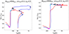 |
Fig. 1. HR diagram for GENEC (red) and MESA (blue) evolution models with 60 M⊙ (left panel) and 200 M⊙ (right panel). Black dots represent the point where Γe = 0.5 and thus the wind regime transits from thin to optically thick, black crosses represent the end of the H-core burning stage, black stars represent the beginning of the He-core burning stage, cyan stars represent the switch between H-rich to H-poor helium stars, and magenta stars represent the end of the He-core burning stage. |
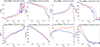 |
Fig. 2. Left panel: Evolution of mass-loss rate, stellar mass, stellar radius, and Eddington factor during the H-core burning stage for GENEC and MESA evolution models with Mzams = 60 M⊙. Right panel: Same as the left panel, but for evolution models with Mzams = 200 M⊙. |
We observe that even though the ZAMS point in the Hertzsrprung-Russell diagram (HRD) is almost the same for the MESA and GENEC tracks, MESA models start with a higher mass loss due to the more rigid effect from Eq. (9), making a difference of ∼0.2 dex in logarithmic scale. However, for our Mzams = 60 M⊙ models, this difference is not large enough to produce significant deviations at the beginning; thus, both tracks move upwards increasing luminosity at temperature nearly constant. Both models reach Γe = 0.5 prior of reaching their maximum radial expansion in the MS, but our GENEC model reaches a higher temperature because of its slightly slower mass loss, its faster rotation, and a more efficient mixing. This is supported by the data given in Table 1, where the MESA model reaches to the switch point from thin to thick winds (black dots in Figures 1 and 2), with lower mass and lower mass fractions of helium and nitrogen, in contrast with the GENEC model. Once the winds for both models become optically thick, the mass loss in both cases is described either by Eq. (5) or V01/GH08 formulae depending on the condition of Teff being higher or lower than 30 kK. Because our GENEC model has a higher luminosity and larger Γe, its optically thick Ṁ will be larger enough to remove more layers and therefore to end the H-core burning stage with less mass than our MESA model (42.1 M⊙ vs. 45 M⊙). However, the most remarkable difference is the final chemical composition at the H-depletion: our GENEC model ends with a helium mass fraction of Ysurf = 0.929. Our results indicate that the stellar structure is almost homogeneous, much more compact (≃5 R⊙), and hotter (Teff ≃ 90 kK).
Properties of our evolution models during the H-core burning stage.
We notice that for both 60 M⊙ models, the transition occurs outside the range of validity of both Ṁthin and Ṁthick, where V01 dominates both wind regimes (see Fig. 1 from Paper I) and the only jump in mass loss is due to the bi-stability jump (Vink et al. 1999), at Teff ≃ 28 kK. Nonetheless, the fact that Γe = 0.5 is reached during the main sequence implies that this point also represents the transition from thin to thick winds, as we discuss in Sect. 4.1.
For our Mzams = 200 M⊙ models, the initial mass loss start around 10−5 M⊙ yr−1 and again the MESA model starts with a higher Ṁ due to Eq. (9). The initial rotational velocity substantially differs between both models, because both models calculate a slightly different starting point for the ZAMS in the HRD as a consequence of both the numerical uncertainties (Agrawal et al. 2022a). We note that these uncertainties tend to increase for larger masses and the different calculation of the critical rotational velocity outlined in Sect. 2.5. Despite these corrections, both models exhibit a very similar track across the HRD, reaching Γe = 0.5 at the very beginning of their lives. Subsequently, the stars spend more than their 90% of their H-core burning lifetime in the optically thick wind regime. Nonetheless, in this mass regime, the mass-loss escalates with metallicity only as Ṁ ∝ Z0.48 (according to Eq. (5)); thus, our initial mass loss for the thick wind regime is around log Ṁ ≃ −4.8, not large enough to produce an abrupt decrease in the luminosity. This is the reason why both tracks keep moving upwards in the HRD diagram until log L/L⊙ ≃ 6.7. Once the mass loss increases enough to stop the rise in luminosity, both models move bluewards keeping L* almost constant. This time, the MESA model drops its rotational velocity slower than the GENEC model, keeping a more moderate radius and ending their H-core burning stage with a larger effective temperature (∼100 kK, against the ∼80 kK from the GENEC model). Despite the fact that our GENEC expanded more redwards, it ends its H-burning with a more advanced chemical enrichment at the surface. Even though this could be partially attributed to the larger initial rotation, it is also because that GENEC implements a more efficient rotational mixing (Meynet & Maeder 2000; Choi et al. 2016).
The correlation between the both tracks shows the most important difference with respect to previous evolution studies adopting V01. Here, it is found that for Mzams = 200 M⊙, the mass loss starts being strong enough to make the star quickly drop in luminosity (Yusof et al. 2013; Sabhahit et al. 2022, 2023; Martinet et al. 2023). Differences in mass loss also carries another important discrepancy with respect previous studies: our models end the H-core burning stage with final masses of ∼100.5 M⊙. This is larger than the Mfinal ≃ 85 M⊙ found by Martinet et al. (2023) for Mzams = 180 M⊙, which is the study with the structure set-up that is closest to ours (αov = 0.2 and Ledoux convection criterion); however, we still adopted old winds. Our result is even more remarkably larger than the Mfinal ≃ 40 M⊙ found by Sabhahit et al. (2022, 2023), who adopted a Ṁthick from Vink et al. (2011). In contrast with these huge mass losses, the models adopting weaker (thin and thick) winds makes a Mzams = 200 M⊙ star lose ‘only’ one half of their mass at the end of H-core burning stage. This signifies an important impact related to the spectroscopic diagnostics to be done over Galactic VMS, as we explain in Sect. 4.3.
3.2. He-core and C-core burning stages
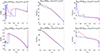 |
Fig. 3. Left panel: Evolution of mass-loss rate, stellar mass, stellar radius, and Eddington factor during the He-core and C-core burning stages for GENEC and MESA evolution models with Mzams = 60 M⊙. Right panel: Same as the left panel, but for evolution models with Mzams = 200 M⊙. |
Given that the star 60 M⊙ from our MESA model ends the MS with a less homogeneous chemical structure (only a ∼57% of helium mass fraction, in contrast with the ∼93% predicted by GENEC), it quickly expands until reaching Teff ≃ 8000 K with a maximum radius of ≃740 R⊙. This is because stars keeping a more constant chemical composition from the core to the surface remain in the bluer part of the HR diagram (Maeder 1987). The beginning of the He-core burning stage (black star symbol in the figures) makes the star return bluewards, thus increasing its temperature and its mass loss. On the contrary, GENEC model predicts a compact star which enters into the He-core burning stage without any radial expansion. This divergence on the models indicate that Mzams ≃ 60 M⊙ represents a threshold for the Hertzsprung-gap: less massive stars will all expand post MS despite minor differences in the rotational mixing, whereas more massive will not (see Fig. 2 from Paper I). These initial differences during He-core ignition later converge into the position at the HRD where both stellar models become H-poor WR stars. Hence, both models show a similar track for the rest of the He-core burning, with a large diminishing in the luminosity from log L/L⊙ ≃ 6.2 to ≃5.75 at temperature almost constant T* ≃ 140 kK. As a consequence, the final masses at the end of the He-core burning stage are relatively the same for MESA and GENEC tracks (≃16.7 M⊙); thus, the remaining evolution through the C-core burning is practically identical for both models.
For the 200 M⊙ case, differences in both the stellar mass and the chemical composition after the H-depletion are almost negligible. It is only the HRD where the He-ignition occurs that is significantly relevant. Because of its proximity to the Eddington limit (with Γe ≃ 0.7) and lower density, the convection at the outer envelope of a star born with Mzams = 200 M⊙ is highly superadiabatic (i.e. the temperature gradient is larger than the adiabatic temperature gradient) and therefore the energy released in the interior remains locked at the sub-surface layers, thus creating numerical instabilities in the models where each evolution code adopts different strategies to handle it (Agrawal et al. 2022b). MESA reduces the superadiabacity in radiatively dominated regions by means of the use_superad_reduction method, which can be interpreted as a lowering in the opacity κ(r) in the sub-surface regions near the Eddington limit (Jermyn et al. 2023). On the contrary, our 200 M⊙ GENEC does not incorporate this superadiabacity rescaling and thus excess in the temperature gradient leads to a considerable inflation when the last traces of hydrogen are removed from the surface and the opacity drastically changes (Yusof et al. 2013; Martinet et al. 2023), until this excess of energy is released due to Supra-Eddington mass loss (Ekström et al. 2012) and the star returns to its initial radius. During this expansion, only less than the 0.1% of the total mass is inflated, keeping the remaining 99.9% of the total mass constrained into the same stellar radius. This is the reason why this expansion should not be considered for any binary interaction Belczynski et al. (2022). Indeed, we show this expansion due to superadiabatic instability as a sudden expansion redwards in the HRD of Fig. 1, but we did not consider it for our plot of radial evolution during the He-core burning (Fig. 3), nor for the maximum radius in Table 2. Moreover, the strategies to deal with these superadiabatic instabilities are approached from a numerical point of view and any possibilities of a physical phenomenon were scarcely considered. After this phenomenon, the star will decrease its luminosity at almost constant temperature until log L/L* ≃ 6.0 according to both MESA and GENEC models, then the He-core burning stage ends with a stellar mass of ≃25.5 M⊙, with the star comprised of a ball of ≃94% carbon and oxygen. We ultimately reach the end of the C-core burning stage with final masses of 24.4 M⊙ according to GENEC and 24.8 M⊙ according to MESA.
Properties of our evolution models during the He-core and C-core burning stages.
4. Theoretical and observational diagnostics
4.1. Self-consistent mass loss close to Γe, trans
As shown in Sect. 2.3, our evolution models use as a criterion to switch from optically thin winds of OB-type stars to thick winds of WR-type stars during the main sequence, the Eddington factor instead of the surface hydrogen abundance. In particular, we used the transition defined by Bestenlehner (2020), which corresponds to the Γe, where the line-driven contribution to the CAK mass-loss equalises with the continuum-driven contribution. Below Γe, trans, the wind is predominantly line-driven and, thus, Ṁ it can be described by our self-consistent m-CAK prescription, whereas over Γe, trans the continuum radiation by electron scattering dominates.
Therefore, a question that arises is how the transition towards thick winds can be approached from self-consistent mass-loss rates at optically thin regime towards Γe, trans. To approach this, we plot in Fig. 4 the Ṁsc as a function of the Eddington factor coming from the models introduced in Gormaz-Matamala et al. (2023), plus the GENEC models introduced in this work. We can see that the Ṁ − Γe easily correlates with a linear fit in the log–log plane, as
 (12)
(12)
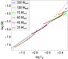 |
Fig. 4. Ṁ − Γe correlations taken from the GENEC self-consistent evolution models from Gormaz-Matamala et al. (2023) and this work. The dashed line represents the best linear fit for these Msc, whereas the gray dot-dashed line represents the fit of Eq. (5) adopted for Z = 0.014. |
This rough fit of Eq. (3) agrees reasonably well with the  from Bestenlehner et al. (2014) and with the
  from (Brands et al. 2022), for the low Eddington factor regime. In other words, Ṁsc behaves as in Eq. (5) when Γe ≲ 0.5, which is appreciated in Fig. 4, where the both fits run in parallel for Γe ≪ 1. It is important to mention that even though the Ṁ − Γe correlation is a very useful tool to describe the escalation of the mass loss in the proximity of the Eddington limit, it is not a formal function. The value of Ṁ may vary for a same value of Γe, if the stellar mass or the luminosity or the hydrogen abundance are different. In particular, the linear behaviour of Ṁsc dissipates as we approach Γe ≃ 0.5, thus suggesting that the m-CAK prescription stops being valid for regimes with larger Eddington factor (where the contribution of the electron scattering to the radiative acceleration becomes more dominant) and a prescription considering optically thick winds needs to be adopted.
We also observe in Fig. 4 that Eqs. (11) and (5) intersect at logΓe ≃ −0.62 (Γe ≃ 0.24), very close to the empirical kink found by Bestenlehner et al. (2014) at logΓe ≃ −0.58. After that point, formula for Ṁthick winds clearly exceeds Ṁthin, finishing with a difference of ≃0.5 dex when Γe = 0.5, as shown in Fig. 2. Hence, we could have a smooth transition from Ṁthin to Ṁthick by simply setting the transition at the point where both formulae intersect. However, we decide for the purposes of this paper to employ Γe, trans as originally set by Bestenlehner (2020), to preserve the physical meaning and exploring the caveats.
The rough fit introduced in Eq. (11) is set for solar metallicity, whereas the fit introduced in Eq. (5) corresponds to the calibration done by Brands et al. (2022) at the LMC metallicity (Z = 0.006). In addition, we include an extra metallicity dependence based on our own prescription. Actually, the general expression derived by Bestenlehner (2020) is
 (13)
(13)
with α being the CAK line-force parameter and Ṁ0 the mass-loss rate at Γe, trans. In principle, we could merge both Eq. (11) and Eq. (5) into one single expression as Eq. (12), by using the tabulated α values from Gormaz-Matamala et al. (2023). In such case, the transition from thin to thick winds would be smooth, given that the continuum already contributes to the wind mass-loss rate even below Γe, trans = 0.5. However, that merging would require the analysis of different metallicities, and the present study is focused on the Milky Way. In a forthcoming paper we aim to explore the possibility of adopting one unique Eq. (12) for both thin and thick winds, together with more self-consistent calculations of the line-force parameters (Gormaz-Matamala et al. 2022a) for stellar models around Γe, trans.
4.2. Eddington factor and wind efficiency
The transition from thin to thick winds based on the proximity of the Eddington factor was recently studied by Gräfener (2021) and Sabhahit et al. (2023). In such studies, the switch from OB to WNh stars is set by using the relationship between the optical depth at the sonic point of the wind structure (τs) and the wind efficiency number (η ≡ Ṁv∞/(L∗/c)) from Gräfener et al. (2017), as follows:
 (14)
(14)
with v∞ and vesc being the wind terminal and the escape velocities, respectively.
Since η denotes the ratio between the mechanical wind momentum and the total momentum of the radiatively-driven wind, the value of η = 1 corresponds to the single scattering limit. If η ≥ 1, it means that photons can be absorbed and re-emitted through the wind structure more than once (Lucy & Abbott 1993). Performed calculations found η ≃ 0.6 as the transition point for Z⊙, based on the mass-loss rates for Galactic and LMC WNh stars (Vink & Gräfener 2012; Sabhahit et al. 2022), plus finding that this ηswitch decreases for lower metallicities (Sabhahit et al. 2023). These calibrations make the value of this transition mass-loss rate, Ṁtrans, being model-independent of factors such as clumping. However, the temporal location of this thin-to-thick transition depends on the evolution of η, which in turns depends on the mass-loss recipe adopted a priori for the initial optically thin regime (V01 for this case, even for Mzams ≃ 40 − 60 M⊙).
On the contrary, the proposed transition towards thicker winds at Γe = κeL*/4πcGM* = 0.5 is explicitly independent on the mass-loss regime adopted for the optically thin regime. In addition, there is no need for any β-law assumption for the velocity profile (Gormaz-Matamala et al. 2022a). In this case, we enter into the optically thick wind regime because the continuum contribution to the radiative-driving mechanism becomes more relevant as we approach the Eddington limit. This is the reason why the Γe, trans is almost constant for different values of α CAK parameter. Hence, this transition differs from the transition based on the single-line scattering limit established by Sabhahit et al. (2022, 2023), where the kink in the Ṁ − Γe is due to the dominance of multi-scattering for the line-driven mechanism. This means, both transitions are connected to a different physical mechanisms at different wind conditions. The existence of the transition at Γe, trans = 0.5, where continuum-driven wind becomes predominant does not contradict the existence of a limit where the line-driving needs to adopt multi-scattering. Indeed, the trend shown in Fig. 5 suggests that the condition η ≃ 0.6 should be satisfied at some point Γe ≫ 0.5, even though it is not possible to assure it properly because of the lack of studies adopting new Ṁ recipes for Γe > 0.4 (Krtička & Kubát 2017; Björklund et al. 2021; Gormaz-Matamala et al. 2023), whereas the transition Eddington factor determined by Sabhahit et al. (2022) is around ∼0.4 (see their Table 3). This implies that either new winds predict a transition wind efficiency lower than the ηswitch found by keeping V01 for thin winds (i.e. meaning that the η transition would depend on the mass-loss recipe adopted for low Γe) or the transition to thick winds might be better represented with the predominance of electron scattering for the radiative acceleration when Eddington factor goes around ∼0.4 − 0.5. As discussed in Sect. 4.1, this is exactly the range of Γe where the self-consistent mass-loss rate shows more dispersion.
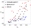 |
Fig. 5. η − Γe correlations taken from theoretical models tabulated by Krtička & Kubát (2017), Björklund et al. (2021), and Gormaz-Matamala et al. (2023). |
Another aspect that should be explored, is the metallicity dependence. Sabhahit et al. (2023) found that the ηswitch value where the wind becomes optically thick varies with the metallicity, given the direct dependence on Ṁ and terminal velocity for the wind efficiency number (Vink & Gräfener 2012) and the adopted scaling for the terminal velocities at a different Z. From our perspective, the transition based on Γe, trans = 0.5 appears to be invariant for different metallicities due to its invariance for different values of the line-force α (which it is metallicity dependent). However, as seen in Sect. 4.1, a deeper analysis of the m-CAK around Γe > 0.4 will be required at various values of Z, both to evaluate the possibilities of some metallicity dependence for Γe, trans but also to get Ṁthick(Z). Up to now, we just have the calibration done by Brands et al. (2022) plus the Ṁ − Z dependence from Gormaz-Matamala et al. (2023), fitted only for the mass range of 25 − 120 M⊙ and thus extrapolated up to Mzams = 200 M⊙ in this work.
For a more general prospective, it is important to mention the increase of the Eddington factor as the star evolves through the main sequence, with weaker winds boosting this tendency for the cases with Mzams ≳ 70 M⊙ (Gormaz-Matamala et al. 2023, Fig. A7). The more massive the star, the faster it reaches Γe, trans = 0.5 and therefore the shortest its fraction of MS lifetime adopting Ṁsc. In the case of the evolution models introduced in this work, a 60 M⊙ star will spend ∼92% of its MS lifetime exhibiting optically thick winds (∼92% for the MESA model), in contrast with the ∼7% of the MS lifetime for a 200 M⊙ star (∼4% for the MESA model). These percentages of the lifetime are given by the location and track across the HRD and not by their Ṁ adopted during the optically thin regime. Therefore, the chosen stellar masses for the analysis in this work represent the approximated limits where optically thin and thick winds can coexist during the main sequence stage. For stars with Mzams < 60 M⊙, the limit Γe = 0.5 may not be reached during the MS and therefore the stars will just become classical WR after the depletion of hydrogen, as in traditional evolution models. On the other limit, for stars with Mzams ≥ 200 M⊙, the condition that Γe = 0.5 from the ZAMS is satisfied; therefore, the wind is fully optically thick, as also found by Sabhahit et al. (2023). In the intermediate-mass range, stars will spend one fraction of their lifetime with thin OB-type winds and reduced mass-loss as reported by Gräfener (2021), and the other fraction with the enhanced Ṁ if they are WNh stars. In summary, the new, weaker winds from Gormaz-Matamala et al. (2022b); Gormaz-Matamala et al. (2023) can be applied for all initial masses for the earliest stages, even for VMS, for the segment of time when Γe < 0.5 is satisfied.
4.3. Spectroscopic analysis
The new mass-loss prescription, along with the new transition from thin to thick winds, modify the evolutionary tracks across the HR diagram and thus the spectroscopic phases. According to the output of our evolution models, we can classify the spectroscopic phases of our evolution models according to
-
O-type: optically thin wind and Teff ≥ 26.3 kK;
-
B-type: optically thin wind and Teff < 26.3 kK;
-
eWNL: WR star with Xsurf ≥ 0.05;
-
eWNE: WR star and Xsurf < 0.05 and (12C + 16O)/4He ≤ 0.03;
-
WC: WR star wind and (12C + 16O)/4He > 0.03;
-
WO: WR star with log Teff ≥ 5.25.
These WR boundaries are derived from the conditions settled by Yusof et al. (2013), Aadland et al. (2022), and Martinet et al. (2023); whereas the distinction between O and B-type is taken from Groh et al. (2014). It is important to note that this classification is not based on spectral analysis but on the output of our theoretical models and, thus, discrepancies may be observed. For example, we separated the evolutionary eWNL and eWNE Foellmi et al. (where ‘e’ stands from evolutionary, following 2003) according to the hydrogen abundance as done by Meynet & Maeder (2003), but the separation between WNL and WNE spectral sub-types is based on the ionisation levels of the surface nitrogen (Smith et al. 1996). This could suggest that all WNE stars are H-poor, although there is evidence of a few H-rich WNE stars in the Milky Way (Hamann et al. 2019). These H-rich WNE stars however, have luminosities below log L*/L⊙ ≃ 5.5, which suggest their progenitors were stars with Mzams ≃ 40 M⊙ (Georgy et al. 2012); thus, they are out of the range of our analysis. Our results are shown in Table 3, whereas the location of these spectral phases across the HRD is shown in Fig. 6.
 |
Fig. 6. Distribution across the HRD of the evolutionary spectral types introduced in Sect. 4.3. The red and blue dots represents time intervals of 20 000 years, starting from the end of the H-core burning, for our GENEC and MESA models, respectively. |
Lifetime predicted by our GENEC and MESA models in the spectroscopic phases according to stellar evolution.
Even though it is not a formal spectroscopic phase, we classify our star as an LBV if the HD-limit (L > 6 × 10⁵ and 10−5L1/2R > 1) is exceeded (Humphreys & Davidson 1994; Hurley et al. 2000). However, we note that recent works have found a lower luminosity limit of L > 3 × 10⁵ (Davies & Beasor 2020). This is particularly evident for our 60 M⊙ MESA model, where the post MS expansion exceeds the HD limit and the star would then spend 12 kyr (0.26% of its total lifetime) as an LBV. Despite this short period, the star had a mass of Mpre, lbv ≃ 44.1 M⊙ and XH ≃ 0.4, to end with Mpost, lbv ≃ 41.9 M⊙ and XH ≃ 0.24. Therefore, it would have experienced an average mass loss of Ṁlbv ≃ 1.8 × 10⁻⁴ M⊙ yr−1 (log Ṁlbv ≃ −3.7). This value is close to the adopted Ṁlbv by Belczynski et al. (2010), but it still comes from the application of the wind recipes of Vink et al. (2001) and de Jager et al. (1988) in a region of the HRD beyond the HD limit. Models for eruptive mass loss (Quataert et al. 2016; Cheng et al. 2024), which are more in agreement with the nature of LBVs, would be more required to better represent the evolution during this phase. In parallel, our 60 M⊙ GENEC does not become an LBV because its more chemically homogeneous structure avoids any radial expansion after the H-depletion. Therefore, despite that the final masses tabulated for both codes are quite similar, the prediction about the existence or not of the LBV phenomenon strongly depends on the calculated mixing during the main sequence stage. In opposition, our 200 M⊙ GENEC evolution track moves redwards, crossing the HD limit, between its phases WNE and WC. This reinforces the uncertain relation of the LBV phenomenon with the evolution of massive stars because, if we consider redwards expansion as a physical phenomenon, instead of a numerical artefact, it would mean that LBV events could occur even after the star becomes a hydrogen-depleted WN star. However, this has never been observationally found and then the idea of a numerical artefact due to a drastic change in the opacity due to the removal of the last traces of hydrogen looks more compelling.
Besides the standard classification for WR stars, in Table 3 and Fig. 6, we also separated the WNL stars with XH > 0.3. Given that typical stellar evolution models enter into the WR phase when either XH < 0.3 (Ekström et al. 2012) or XH < 0.4 Brott et al. (2011), this distinction is made to incorporate the WNh stars, whose optically thick winds are because of the proximity to the Eddington limit before the H-depletion, according to the criterion Γe ≥ 0.5 established in Sect. 2.3. Thus we discern from the WNL stars which are result of the ‘classical’ evolution, where the star becomes a WR due to the drift bluewards after the LBV episodes during the He-core burning stage (Conti 1975; Groh et al. 2014). Indeed, WNh stars with XH ≥ 0.3 are constrained to a very narrow band of temperature in the HRD, log Teff ≃ 4.5 − 4.7 (Martins et al. 2008; Crowther et al. 2010; Hamann et al. 2019), whereas WNL stars with XH ≤ 0.3 are spread across a wider range of temperatures (Martins 2023). To better illustrate this point, we selected the Galactic WNh stars (with XH ≥ 0.3) from the Arches cluster (Martins et al. 2008), from the NGC 3603 cluster (Crowther et al. 2010), and from the local neighbourhood (Hamann et al. 2019). We give these stars in Table 4. In addition, we plot our GENEC and MESA models for 60 and 200 M⊙, highlighting the segments where Γe ≥ 0.5 and XH ≥ 0.3. The results are shown in Fig. 7. Despite the limited differences between the evolution tracks, our prescription adequately describes the narrow band where WNh stars exist, meaning they are the product of stars born with Mzams ≳ 60 M⊙ producing optically thick winds before the H-depletion due to their proximity to the Eddington limit. In the middle panel, we append models for 100 M⊙, indicating that the thick band also fits the WNh stars of our sample.
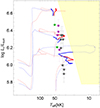 |
Fig. 7. Evolutionary GENEC and MESA tracks for 60 and 200 M⊙ from Fig. 1 and additional 100 M⊙ models, where the thick solid lines represent the segments where the wind is optically thick (Γe ≥ 0.5) and Xsurf ≥ 0.3. The gray stars correspond to the sample of WNh stars from Martins et al. (2008), the purple stars to the sample of Crowther et al. (2010) and the green stars to the sample of Hamann et al. (2019), tabulated in Table 4. Yellow shadowed area correspond to the HRD region where the HD limit is exceeded. |
For the 200 M⊙ cases the observational diagnostics are more uncertain. For instance, the stars tabulated in Table 4 are also the brightest WNh stars in the Milky Way and none of them reach the luminosity of log L*/log L⊙ ≳ 6.55. The early approaching to the Eddington limit from the very beginning of the main sequence implies that the O-type phase in our models is very short; therefore, the star will spend the largest percentage of their lifetime (almost a ∼90% for both models) as a WNh. This is a remarkable difference with respect to previous studies, where very massive stars have spent the majority of their lifetime as O-type stars, until they remove more than the half of their initial surface H abundance (Martinet et al. 2023). In other words, our models predict that extremely luminous Galactic stars have more probabilities of being WNh than O-type. The star W49-#2, with log L*/L⊙ ≃ 6.64 ± 0.25 (one of the brightest stars known in the Milky Way) is classified as O2–3.5If* (Wu et al. 2016) but quite close of being a Of/WN star based on the spectral classification of Crowther & Walborn (2011). In any case, the high stellar mass (∼250 M⊙) estimated by Wu et al. (2016) implies Γe ≃ 0.35 − 0.46 (depending on the XH to be considered in Eq. (2)); thus, it is not close enough to the Eddington limit to develop optically thick winds.
Beyond WNh stars, our new evolution models for 200 M⊙ also predicts the existence of H-poor WR stars with luminosities greater than log L*/L⊙ > 6.0, which is same as in the rotating models of 180 M⊙ and 250 M⊙ from Martinet et al. (2023). If we sum up the lifetime of eWNE, WC and WO spectroscopic phases from Table 3, we find that the our 200 M⊙ models will have spent ∼14% of their lifetime according to the GENEC model (∼13% in the case of MESA), which is very close to the ∼11% for the same phases predicted by them. Such small discrepancy can be easily explained by our choice of setting eWNE for Xsurf ≤ 0.5 (Yusof et al. 2013, from) instead of ≤10−5, which implies that eWNE will form around the ∼3.5% of the total lifetime (either H-rich or H-poor), in contrast with the absence of eWNE phase for 200 M⊙ from Martinet et al. (2023). Nonetheless, only two WN (WR 18 and WR 37) stars with XH = 0 satisfy log L*/L⊙ > 6.0 in the Galactic catalog of Hamann et al. (2019); whereas for WC type, WR 126 is the only WN/WC star with log L*/L⊙ > 6.0 in the Milky Way (Sander et al. 2019). However, the trace of the red and blue dots from Fig. 6 confirms that eWNE is a very short period and these stars quickly drop their luminosities from log L*/L⊙ ≥ 6.6 to ≃6.0 in just ∼200 kyr. Even though the aforementioned catalogs still cover a small region of the Milky Way, the absence of WNE and WC stars with log L*/L⊙ ≥ 6.1 (which should be evolved from models born with masses ≃60) should suggest that Eq. (5) might be underestimating the actual value of the mass-loss rate for the most massive H-rich WN stars (as a consequence of the extrapolation up to 200 M⊙ mentioned in Sect. 4.2). Even though it is still possible that we might have been underestimating the actual value of the mass-loss rate for the most massive H-rich WN stars as a result, it is important to mention that our Galactic WR catalogs are still quite constrained to our solar neighbourhood. The study and discoveries of new sources at the edge of the known stellar luminosities, together with less uncertain data, is beyond the scope of this paper.
5. Summary and conclusions
In Paper I we explored the expected final masses prior to the core collapse, where we calculated stellar evolution updating the mass-loss prescription. In this work, we confirm the importance of these new wind prescriptions by analysing its impact over the expected spectroscopic stages (OB-type, WNh and classical WR).
Regardless of the unification of the overshooting (αov = 0.5), the rotation (ω/ωcrit = 0.4), the angular momentum transport (Tayler-Spruit dynamo), the convective boundary criterion (Ledoux), and the line-driven mass-loss prescriptions for both the GENEC and MESA codes, there are important differences between the calculated evolutionary tracks. For instance, GENEC computes a more prominent rotational mixing during the main sequence phase, leading to a more homogeneous stellar structure at the H-core depletion in comparison with MESA. This is particularly evident for our 60 M⊙ models, where our less homogeneous model largely expands and crosses the HD limit before the He-ignition. Such a discrepancy between both models can be interpreted as a boundary in the mass range below which stars normally expand and over which stars maintain a moderate size because of the strong outflows (Romagnolo et al. 2023). For the 200 M⊙ models, due to the large size of the convective core, the differences between both evolution codes are less relevant. Thus, it is the treatment for superadiabacity during the He-core burning phase that continues to be a matter of debate.
Concerning stellar masses, both GENEC and MESA codes show similar results at the end of each core-burning process, with the most remarkable mass losses during the post-main sequence stages. Models with Mzams = 60 M⊙ end the H-core burning phase, with final masses of 42.1 and 44.5 M⊙, respectively. Subsequently, they experience strong outflows during He-core burning stages to finish with 16.1 M⊙ at the C-core depletion. This is a striking discrepancy with the Mbh ≃ 30 M⊙ found at Mzams = 60 M⊙ by Bavera et al. (2023), where the rotational effects were not considered, or with Vink et al. (2024), where the WR stage is absent for Mzams = 40 M⊙. For our 200 M⊙ case, where the main sequence is almost fully dominated by thick winds, both GENEC and MESA models predict a final mass of ∼100 M⊙ at the end of the H-core burning stage, ending later with Mfin ≃ 24.6 M⊙ at the C-core depletion. This result is also largely discrepant with other studies such as Yusof et al. (2013) or Sabhahit et al. (2022, 2023), who found that a star with Mzams = 200 M⊙ would lose almost the ∼80% of its mass during the H-burning stage only. Despite the discussion introduced in Section 4.1, such difference in the calculated mass remnants is not produced due to the approach of the transition from thin to thick winds close to the Eddington factor, but due to the lower recipes for Ṁ for both thin (Gormaz-Matamala et al. 2023), instead of V01, and thick Bestenlehner (2020), instead of the Vink et al. (2011) wind regimes.
However, the most remarkable result is that our transition between the optically thin winds of OB-type stars and the thick winds of WNh stars (based on the dominance of electron scattering over line-driving) results in the prediction of a band in the HRD where stars are expected to develop optically thick winds, but with large hydrogen fractions at the surface (Xsurf ≫ 0.3). This band corresponds to effective temperatures between log Teff ≃ 4.5 − 4.7. This is in agreement with the spectroscopic diagnostics of Martins et al. (2008), Crowther et al. (2010), and Hamann et al. (2019). The basis for the proposed switch of wind regime at Γe, trans = 0.5 follows the formulation of Bestenlehner (2020) based on CAK theory and it considers that at early evolutionary stages, the Ṁ values for regular massive stars (i.e. not VMS) are about three times lower than the traditionally assumed for V01. This statement is compatible with the idea of having WNh stars born from Mzams ≃ 60 M⊙, whereas we find reduced Ṁ from hydrodynamic analysis on winds for the same mass range (Sander et al. 2017; Gormaz-Matamala et al. 2021). As we escalate in the mass range, the fraction of MS time at which the stellar wind is optically thin becomes shorter; therefore, the wind of very massive stars posses enhanced values of mass-loss rates because they spent larger fractions of their MS dominated by thick winds. Stars at Mzams ≳ 200 M⊙ are already dominated by thick winds from the very beginning of their lifetimes, similarly to the reports in Sabhahit et al. (2023).
The implementation of Γe = L*κe/4πcGM* instead of η = Ṁv∞/(L∗/c) is explicitly independent of the adopted Ṁ recipe for thin winds, thus less dependent on the mass-loss history before the O/WNh transition. The value log Ṅthick(Γe,trans = 0.5) ∼ − 4.9 is in line with the so-called ‘model-independent’ mass-loss transition from Vink & Gräfener (2012); however, we note there is a difference of ∼0.5 dex for Ṁthin at larger values of Γe. This disagreement could be avoided by putting the value of Γe, trans down to ∼0.24, but for the purposes of this study, we kept Γe, trans = 0.5 to preserve the physical meaning of an equilibrium between the line-driven and the electron scattering to the total radiative acceleration. To better connect the new recipes for O-type stellar winds with the enhanced winds of WNh stars, w ought to expand the self-consistent wind calculations of Krtička & Kubát (2017) or Gormaz-Matamala et al. (2021) for Γe ≫ 0.4, exploring the evolution of the resulting η from ZAMS to the O/WNh transition.
This work focuses on calculations applicable to stars with solar metallicity and in earlier stages of evolution. However, recent observations reveal a significant population of Wolf-Rayet stars (WNh) in young and metal-poor clusters such as R136 (Brands et al. 2022) and 30 Dor Ramírez-Agudelo et al. (2017), both located in the LMC. This necessitates extending our procedures and diagnostics to include very massive stars with metallicities as low as Z ≲ 0.006, as suggested by Martins & Palacios (2022). Additionally, these upgrades in mass-loss prescriptions need to be applicable to stars with Teff ≤ 30 kK. Evaluating approaches such as those proposed by Krtička et al. (2024) for B-supergiants is a promising avenue for future works, together with incorporating more detailed prescriptions for the stellar interiors based on the state-of-the-art asteroseismology (Pedersen et al. 2021). Finally, we must also consider that the constraints on stellar parameters and mass-loss rates of massive stars in metal poor environments still make up an active field of research (Sander et al. 2024; Verhamme et al. 2024; Backs et al. 2024; Gómez-González et al. 2025).
Nevertheless, evolution models used to both V01 and GH08 to describe mass loss from WR winds, depending on which recipe provided the largest Ṁ at certain point (Yusof et al. 2013).
Notice that, because of this definition, the Eddington limit only applies for the stellar surface.
Do not confuse this parameter, α, which is one of the line-force parameters from CAK theory (Castor et al. 1975; Abbott 1982), with the αov for the convective core overshooting.
In this work, we denote Ω to the ratio between rotational velocity and critical velocity following the formalism of the line-driven theory (Curé & Rial 2004; Puls et al. 2008; Venero et al. 2024), whereas for the angular velocity we use the ω.
Acknowledgments
We thank to the anonymous second referee for their valuable comments and feedback, together with to Joachim Bestenlehner, Sylvia Ekström, and Michel Curé for the fruitful discussions. Authors acknowledge support from the Polish National Science Center grant Maestro (2018/30/A/ST9/00050). The authors also thank the GENEC and MESA communities at large for their helpful feedback on the models creation. Computations for this article have been performed using the computer cluster at CAMK PAN. ACGM thanks the support from project 10108195 MERIT (MSCA-COFUND Horizon Europe). We dedicate this paper to Krzysztof Belczyński, who contributed to this research before his untimely passing on 13th January 2024.
References
- Aadland, E., Massey, P., Hillier, D. J., et al. 2022, ApJ, 931, 157 [NASA ADS] [CrossRef] [Google Scholar]
- Abbott, D. C. 1982, ApJ, 259, 282 [Google Scholar]
- Abbott, B. P., Abbott, R., Abbott, T. D., et al. 2016, Phys. Rev. Lett., 116, 061102 [Google Scholar]
- Abbott, R., Abbott, T. D., Abraham, S., et al. 2021, ApJ, 913, L7 [NASA ADS] [CrossRef] [Google Scholar]
- Agrawal, P., Hurley, J., Stevenson, S., Szécsi, D., & Flynn, C. 2020, MNRAS, 497, 4549 [NASA ADS] [CrossRef] [Google Scholar]
- Agrawal, P., Szécsi, D., Stevenson, S., Eldridge, J. J., & Hurley, J. 2022a, MNRAS, 512, 5717 [NASA ADS] [CrossRef] [Google Scholar]
- Agrawal, P., Stevenson, S., Szécsi, D., & Hurley, J. 2022b, A&A, 668, A90 [NASA ADS] [CrossRef] [EDP Sciences] [Google Scholar]
- Araya, I., Curé, M., ud-Doula, A., Santillán, A., & Cidale, L. 2018, MNRAS, 477, 755 [NASA ADS] [CrossRef] [Google Scholar]
- Asplund, M., Grevesse, N., Sauval, A. J., & Scott, P. 2009, ARA&A, 47, 481 [NASA ADS] [CrossRef] [Google Scholar]
- Backs, F., Brands, S. A., de Koter, A., et al. 2024, A&A, 692, A88 [NASA ADS] [CrossRef] [EDP Sciences] [Google Scholar]
- Baraffe, I., Clarke, J., Morison, A., et al. 2023, MNRAS, 519, 5333 [NASA ADS] [CrossRef] [Google Scholar]
- Bavera, S. S., Fragos, T., Zapartas, E., et al. 2023, Nat. Astron., 7, 1090 [NASA ADS] [CrossRef] [Google Scholar]
- Belczynski, K., Bulik, T., Fryer, C. L., et al. 2010, ApJ, 714, 1217 [NASA ADS] [CrossRef] [Google Scholar]
- Belczynski, K., Hirschi, R., Kaiser, E. A., et al. 2020a, ApJ, 890, 113 [NASA ADS] [CrossRef] [Google Scholar]
- Belczynski, K., Klencki, J., Fields, C. E., et al. 2020b, A&A, 636, A104 [NASA ADS] [CrossRef] [EDP Sciences] [Google Scholar]
- Belczynski, K., Romagnolo, A., Olejak, A., et al. 2022, ApJ, 925, 69 [NASA ADS] [CrossRef] [Google Scholar]
- Bestenlehner, J. M. 2020, MNRAS, 493, 3938 [Google Scholar]
- Bestenlehner, J. M., Gräfener, G., Vink, J. S., et al. 2014, A&A, 570, A38 [NASA ADS] [CrossRef] [EDP Sciences] [Google Scholar]
- Björklund, R., Sundqvist, J. O., Puls, J., & Najarro, F. 2021, A&A, 648, A36 [EDP Sciences] [Google Scholar]
- Björklund, R., Sundqvist, J. O., Singh, S. M., Puls, J., & Najarro, F. 2023, A&A, 676, A109 [NASA ADS] [CrossRef] [EDP Sciences] [Google Scholar]
- Bouret, J. C., Lanz, T., & Hillier, D. J. 2005, A&A, 438, 301 [NASA ADS] [CrossRef] [EDP Sciences] [Google Scholar]
- Brands, S. A., de Koter, A., Bestenlehner, J. M., et al. 2022, A&A, 663, A36 [Google Scholar]
- Brott, I., de Mink, S. E., Cantiello, M., et al. 2011, A&A, 530, A115 [NASA ADS] [CrossRef] [EDP Sciences] [Google Scholar]
- Castor, J. I., Abbott, D. C., & Klein, R. I. 1975, ApJ, 195, 157 [Google Scholar]
- Chen, Y., Bressan, A., Girardi, L., et al. 2015, MNRAS, 452, 1068 [Google Scholar]
- Cheng, S. J., Goldberg, J. A., Cantiello, M., et al. 2024, ApJ, 974, 270 [NASA ADS] [CrossRef] [Google Scholar]
- Choi, J., Dotter, A., Conroy, C., et al. 2016, ApJ, 823, 102 [Google Scholar]
- Conti, P. S. 1975, MSRSL, 9, 193 [NASA ADS] [Google Scholar]
- Crowther, P. A. 2007, ARA&A, 45, 177 [Google Scholar]
- Crowther, P. A., & Walborn, N. R. 2011, MNRAS, 416, 1311 [Google Scholar]
- Crowther, P. A., Schnurr, O., Hirschi, R., et al. 2010, MNRAS, 408, 731 [Google Scholar]
- Curé, M. 2004, ApJ, 614, 929 [CrossRef] [Google Scholar]
- Curé, M., & Rial, D. F. 2004, A&A, 428, 545 [NASA ADS] [CrossRef] [EDP Sciences] [Google Scholar]
- Davies, B., & Beasor, E. R. 2020, MNRAS, 493, 468 [NASA ADS] [CrossRef] [Google Scholar]
- de Burgos, A., Keszthelyi, Z., Simón-Díaz, S., & Urbaneja, M. A. 2024, A&A, 687, L16 [NASA ADS] [CrossRef] [EDP Sciences] [Google Scholar]
- de Jager, C., Nieuwenhuijzen, H., & van der Hucht, K. A. 1988, A&AS, 72, 259 [NASA ADS] [Google Scholar]
- Eggenberger, P., Meynet, G., Maeder, A., et al. 2008, Ap&SS, 316, 43 [Google Scholar]
- Eggenberger, P., Ekström, S., Georgy, C., et al. 2021, A&A, 652, A137 [NASA ADS] [CrossRef] [EDP Sciences] [Google Scholar]
- Ekström, S., Meynet, G., Maeder, A., & Barblan, F. 2008, A&A, 478, 467 [Google Scholar]
- Ekström, S., Georgy, C., Eggenberger, P., et al. 2012, A&A, 537, A146 [Google Scholar]
- Farrell, E., Groh, J. H., Hirschi, R., et al. 2021, MNRAS, 502, L40 [NASA ADS] [CrossRef] [Google Scholar]
- Foellmi, C., Moffat, A. F. J., & Guerrero, M. A. 2003, MNRAS, 338, 1025 [NASA ADS] [CrossRef] [Google Scholar]
- Friend, D. B., & Abbott, D. C. 1986, ApJ, 311, 701 [Google Scholar]
- Fryer, C. L., Olejak, A., & Belczynski, K. 2022, ApJ, 931, 94 [NASA ADS] [CrossRef] [Google Scholar]
- Gaia Collaboration (Panuzzo, P., et al.) 2024, A&A, 686, L2 [NASA ADS] [CrossRef] [EDP Sciences] [Google Scholar]
- Georgy, C., Meynet, G., & Maeder, A. 2011, A&A, 527, A52 [NASA ADS] [CrossRef] [EDP Sciences] [Google Scholar]
- Georgy, C., Ekström, S., Meynet, G., et al. 2012, A&A, 542, A29 [NASA ADS] [CrossRef] [EDP Sciences] [Google Scholar]
- Georgy, C., Saio, H., & Meynet, G. 2014, MNRAS, 439, L6 [Google Scholar]
- Gómez-González, V. M. A., Oskinova, L. M., Hamann, W. R., et al. 2025, A&A, 695, A197 [NASA ADS] [CrossRef] [EDP Sciences] [Google Scholar]
- Gormaz-Matamala, A. C., Curé, M., Cidale, L. S., & Venero, R. O. J. 2019, ApJ, 873, 131 [NASA ADS] [CrossRef] [Google Scholar]
- Gormaz-Matamala, A. C., Curé, M., Hillier, D. J., et al. 2021, ApJ, 920, 64 [NASA ADS] [CrossRef] [Google Scholar]
- Gormaz-Matamala, A. C., Curé, M., Lobel, A., et al. 2022a, A&A, 661, A51 [NASA ADS] [CrossRef] [EDP Sciences] [Google Scholar]
- Gormaz-Matamala, A. C., Curé, M., Meynet, G., et al. 2022b, A&A, 665, A133 [NASA ADS] [CrossRef] [EDP Sciences] [Google Scholar]
- Gormaz-Matamala, A. C., Cuadra, J., Meynet, G., & Curé, M. 2023, A&A, 673, A109 [NASA ADS] [CrossRef] [EDP Sciences] [Google Scholar]
- Gormaz-Matamala, A. C., Cuadra, J., Ekström, S., et al. 2024, A&A, 687, A290 [NASA ADS] [CrossRef] [EDP Sciences] [Google Scholar]
- Gräfener, G. 2021, A&A, 647, A13 [NASA ADS] [CrossRef] [EDP Sciences] [Google Scholar]
- Gräfener, G., & Hamann, W. R. 2008, A&A, 482, 945 [Google Scholar]
- Gräfener, G., Vink, J. S., de Koter, A., & Langer, N. 2011, A&A, 535, A56 [NASA ADS] [CrossRef] [EDP Sciences] [Google Scholar]
- Gräfener, G., Owocki, S. P., Grassitelli, L., & Langer, N. 2017, A&A, 608, A34 [NASA ADS] [CrossRef] [EDP Sciences] [Google Scholar]
- Groh, J. H., Meynet, G., Ekström, S., & Georgy, C. 2014, A&A, 564, A30 [NASA ADS] [CrossRef] [EDP Sciences] [Google Scholar]
- Hamann, W. R., Gräfener, G., Liermann, A., et al. 2019, A&A, 625, A57 [NASA ADS] [CrossRef] [EDP Sciences] [Google Scholar]
- Hawcroft, C., Sana, H., Mahy, L., et al. 2021, A&A, 655, A67 [NASA ADS] [CrossRef] [EDP Sciences] [Google Scholar]
- Hawcroft, C., Mahy, L., Sana, H., et al. 2024, A&A, 690, A126 [NASA ADS] [CrossRef] [EDP Sciences] [Google Scholar]
- Heger, A., Fryer, C. L., Woosley, S. E., Langer, N., & Hartmann, D. H. 2003, ApJ, 591, 288 [CrossRef] [Google Scholar]
- Heger, A., Woosley, S. E., & Spruit, H. C. 2005, ApJ, 626, 350 [Google Scholar]
- Higgins, E. R., Sander, A. A. C., Vink, J. S., & Hirschi, R. 2021, MNRAS, 505, 4874 [NASA ADS] [CrossRef] [Google Scholar]
- Huang, W., Gies, D. R., & McSwain, M. V. 2010, ApJ, 722, 605 [Google Scholar]
- Humphreys, R. M., & Davidson, K. 1994, PASP, 106, 1025 [NASA ADS] [CrossRef] [Google Scholar]
- Humphreys, R. M., Weis, K., Davidson, K., & Gordon, M. S. 2016, ApJ, 825, 64 [NASA ADS] [CrossRef] [Google Scholar]
- Hurley, J. R., Pols, O. R., & Tout, C. A. 2000, MNRAS, 315, 543 [Google Scholar]
- Ivanova, N., Justham, S., Chen, X., et al. 2013, A&ARv, 21, 59 [Google Scholar]
- Jermyn, A. S., Bauer, E. B., Schwab, J., et al. 2023, ApJS, 265, 15 [NASA ADS] [CrossRef] [Google Scholar]
- Josiek, J., Ekström, S., & Sander, A. A. C. 2024, A&A, 688, A71 [NASA ADS] [CrossRef] [EDP Sciences] [Google Scholar]
- Köhler, K., Langer, N., de Koter, A., et al. 2015, A&A, 573, A71 [NASA ADS] [CrossRef] [EDP Sciences] [Google Scholar]
- Krtička, J., & Kubát, J. 2017, A&A, 606, A31 [NASA ADS] [CrossRef] [EDP Sciences] [Google Scholar]
- Krtička, J., & Kubát, J. 2018, A&A, 612, A20 [NASA ADS] [CrossRef] [EDP Sciences] [Google Scholar]
- Krtička, J., Kubát, J., & Krtičková, I. 2024, A&A, 681, A29 [NASA ADS] [CrossRef] [EDP Sciences] [Google Scholar]
- Langer, N. 1997, in Luminous Blue Variables: Massive Stars in Transition, eds. A. Nota, & H. Lamers, ASP Conf. Ser., 120, 83 [Google Scholar]
- Langer, N. 1998, A&A, 329, 551 [NASA ADS] [Google Scholar]
- Ledoux, P. 1947, ApJ, 105, 305 [NASA ADS] [CrossRef] [Google Scholar]
- Lucy, L. B., & Abbott, D. C. 1993, ApJ, 405, 738 [Google Scholar]
- Lucy, L. B., & Solomon, P. M. 1970, ApJ, 159, 879 [Google Scholar]
- Maeder, A. 1987, A&A, 178, 159 [NASA ADS] [Google Scholar]
- Maeder, A., & Meynet, G. 2000, A&A, 361, 159 [NASA ADS] [Google Scholar]
- Martinet, S., Meynet, G., Ekström, S., et al. 2021, A&A, 648, A126 [NASA ADS] [CrossRef] [EDP Sciences] [Google Scholar]
- Martinet, S., Meynet, G., Ekström, S., Georgy, C., & Hirschi, R. 2023, A&A, 679, A137 [NASA ADS] [CrossRef] [EDP Sciences] [Google Scholar]
- Martins, F. 2023, A&A, 680, A22 [NASA ADS] [CrossRef] [EDP Sciences] [Google Scholar]
- Martins, F., & Palacios, A. 2022, A&A, 659, A163 [NASA ADS] [CrossRef] [EDP Sciences] [Google Scholar]
- Martins, F., Hillier, D. J., Paumard, T., et al. 2008, A&A, 478, 219 [NASA ADS] [CrossRef] [EDP Sciences] [Google Scholar]
- Meynet, G., & Maeder, A. 2000, A&A, 361, 101 [NASA ADS] [Google Scholar]
- Meynet, G., & Maeder, A. 2003, A&A, 404, 975 [NASA ADS] [CrossRef] [EDP Sciences] [Google Scholar]
- Meynet, G., Maeder, A., Schaller, G., Schaerer, D., & Charbonnel, C. 1994, A&AS, 103, 97 [Google Scholar]
- Muijres, L. E., de Koter, A., Vink, J. S., et al. 2011, A&A, 526, A32 [NASA ADS] [CrossRef] [EDP Sciences] [Google Scholar]
- Nugis, T., & Lamers, H. J. G. L. M. 2002, A&A, 389, 162 [EDP Sciences] [Google Scholar]
- Olejak, A., Belczynski, K., & Ivanova, N. 2021, A&A, 651, A100 [NASA ADS] [CrossRef] [EDP Sciences] [Google Scholar]
- Olejak, A., Fryer, C. L., Belczynski, K., & Baibhav, V. 2022, MNRAS, 516, 2252 [NASA ADS] [CrossRef] [Google Scholar]
- Pauli, D., Oskinova, L. M., Hamann, W. R., et al. 2022, A&A, 659, A9 [NASA ADS] [CrossRef] [EDP Sciences] [Google Scholar]
- Paxton, B., Bildsten, L., Dotter, A., et al. 2011, ApJS, 192, 3 [Google Scholar]
- Paxton, B., Cantiello, M., Arras, P., et al. 2013, ApJS, 208, 4 [Google Scholar]
- Paxton, B., Marchant, P., Schwab, J., et al. 2015, ApJS, 220, 15 [Google Scholar]
- Paxton, B., Schwab, J., Bauer, E. B., et al. 2018, ApJS, 234, 34 [NASA ADS] [CrossRef] [Google Scholar]
- Paxton, B., Smolec, R., Schwab, J., et al. 2019, ApJS, 243, 10 [Google Scholar]
- Pedersen, M. G., Aerts, C., Pápics, P. I., et al. 2021, Nat. Astron., 5, 715 [NASA ADS] [CrossRef] [Google Scholar]
- Puls, J., Vink, J. S., & Najarro, F. 2008, Astron. Astrophys. Rev., 16, 209 [Google Scholar]
- Quataert, E., Fernández, R., Kasen, D., Klion, H., & Paxton, B. 2016, MNRAS, 458, 1214 [NASA ADS] [CrossRef] [Google Scholar]
- Ramírez-Agudelo, O. H., Sana, H., de Koter, A., et al. 2017, A&A, 600, A81 [NASA ADS] [CrossRef] [EDP Sciences] [Google Scholar]
- Romagnolo, A., Belczynski, K., Klencki, J., et al. 2023, MNRAS, 525, 706 [NASA ADS] [CrossRef] [Google Scholar]
- Romagnolo, A., Gormaz-Matamala, A. C., & Belczynski, K. 2024, ApJ, 964, L23 [NASA ADS] [CrossRef] [Google Scholar]
- Romagnolo, A., Klencki, J., Vigna-Gomez, A., & Belczynski, K. 2025, A&A, 693, A137 [NASA ADS] [CrossRef] [EDP Sciences] [Google Scholar]
- Sabhahit, G. N., Vink, J. S., Higgins, E. R., & Sander, A. A. C. 2022, MNRAS, 514, 3736 [NASA ADS] [CrossRef] [Google Scholar]
- Sabhahit, G. N., Vink, J. S., Sander, A. A. C., & Higgins, E. R. 2023, MNRAS, 524, 1529 [NASA ADS] [CrossRef] [Google Scholar]
- Sander, A. A. C., & Vink, J. S. 2020, MNRAS, 499, 873 [Google Scholar]
- Sander, A. A. C., Hamann, W.-R., Todt, H., Hainich, R., & Shenar, T. 2017, A&A, 603, A86 [NASA ADS] [CrossRef] [EDP Sciences] [Google Scholar]
- Sander, A. A. C., Hamann, W. R., Todt, H., et al. 2019, A&A, 621, A92 [NASA ADS] [CrossRef] [EDP Sciences] [Google Scholar]
- Sander, A. A. C., Vink, J. S., & Hamann, W. R. 2020, MNRAS, 491, 4406 [Google Scholar]
- Sander, A. A. C., Lefever, R. R., Poniatowski, L. G., et al. 2023, A&A, 670, A83 [NASA ADS] [CrossRef] [EDP Sciences] [Google Scholar]
- Sander, A. A. C., Bouret, J. C., Bernini-Peron, M., et al. 2024, A&A, 689, A30 [NASA ADS] [CrossRef] [EDP Sciences] [Google Scholar]
- Scott, L. J. A., Hirschi, R., Georgy, C., et al. 2021, MNRAS, 503, 4208 [NASA ADS] [CrossRef] [Google Scholar]
- Sibony, Y., Georgy, C., Ekström, S., & Meynet, G. 2023, A&A, 680, A101 [NASA ADS] [CrossRef] [EDP Sciences] [Google Scholar]
- Smith, L. F., Shara, M. M., & Moffat, A. F. J. 1996, MNRAS, 281, 163 [NASA ADS] [CrossRef] [Google Scholar]
- Spera, M., & Mapelli, M. 2017, MNRAS, 470, 4739 [Google Scholar]
- Spruit, H. C. 2002, A&A, 381, 923 [CrossRef] [EDP Sciences] [Google Scholar]
- Sundqvist, J. O., Björklund, R., Puls, J., & Najarro, F. 2019, A&A, 632, A126 [NASA ADS] [CrossRef] [EDP Sciences] [Google Scholar]
- Šurlan, B., Hamann, W. R., Aret, A., et al. 2013, A&A, 559, A130 [NASA ADS] [CrossRef] [EDP Sciences] [Google Scholar]
- Tayler, R. J. 1973, MNRAS, 161, 365 [CrossRef] [Google Scholar]
- Tehrani, K. A., Crowther, P. A., Bestenlehner, J. M., et al. 2019, MNRAS, 484, 2692 [NASA ADS] [CrossRef] [Google Scholar]
- Venero, R. O. J., Curé, M., Puls, J., et al. 2024, MNRAS, 527, 93 [Google Scholar]
- Verhamme, O., Sundqvist, J., de Koter, A., et al. 2024, A&A, 692, A91 [NASA ADS] [CrossRef] [EDP Sciences] [Google Scholar]
- Vink, J. S. 2017, A&A, 607, L8 [NASA ADS] [CrossRef] [EDP Sciences] [Google Scholar]
- Vink, J. S. 2022, ARA&A, 60, 203 [NASA ADS] [CrossRef] [Google Scholar]
- Vink, J. S., & Gräfener, G. 2012, ApJ, 751, L34 [Google Scholar]
- Vink, J. S., de Koter, A., & Lamers, H. J. G. L. M. 1999, A&A, 350, 181 [Google Scholar]
- Vink, J. S., de Koter, A., & Lamers, H. J. G. L. M. 2001, A&A, 369, 574 [NASA ADS] [CrossRef] [EDP Sciences] [Google Scholar]
- Vink, J. S., Muijres, L. E., Anthonisse, B., et al. 2011, A&A, 531, A132 [NASA ADS] [CrossRef] [EDP Sciences] [Google Scholar]
- Vink, J. S., Higgins, E. R., Sander, A. A. C., & Sabhahit, G. N. 2021, MNRAS, 504, 146 [NASA ADS] [CrossRef] [Google Scholar]
- Vink, J. S., Sabhahit, G. N., & Higgins, E. R. 2024, A&A, 688, L10 [NASA ADS] [CrossRef] [EDP Sciences] [Google Scholar]
- Wu, S.-W., Bik, A., Bestenlehner, J. M., et al. 2016, A&A, 589, A16 [NASA ADS] [CrossRef] [EDP Sciences] [Google Scholar]
- Yoon, S. C., Woosley, S. E., & Langer, N. 2010, ApJ, 725, 940 [NASA ADS] [CrossRef] [Google Scholar]
- Yungelson, L. R., van den Heuvel, E. P. J., Vink, J. S., Portegies Zwart, S. F., & de Koter, A. 2008, A&A, 477, 223 [NASA ADS] [CrossRef] [EDP Sciences] [Google Scholar]
- Yusof, N., Hirschi, R., Meynet, G., et al. 2013, MNRAS, 433, 1114 [NASA ADS] [CrossRef] [Google Scholar]
Appendix A: Effects of TS dynamo for angular momentum transport
For our GENEC models, we included Tayler-Spruit dynamo (Tayler 1973; Spruit 2002; Heger et al. 2005) for the treatment of the angular momentum transport, in addition to adopting Ledoux instead of Schwarzschild criterion for the treatment of convective layers (Martinet et al. 2023). The evolution during the MS phase is basically not affected by differences in convection treatment, and just for the H-core burning the Ledoux criterion improves the agreement between models and observations for the surface abundances of BSGs evolving back from RSGs (Georgy et al. 2014). For stars with Mzams ≥ 60 M⊙ (as in this study), the impact of the different convective criterion is almost negligible because mass loss become the main driver of the evolution (Sibony et al. 2023).
In Fig. A.1, we show the evolution tracks of our models shown in Section 3, compared to models with the same input but adopting the original inner structure of GENEC. The initial rotation this time follows the framework Ω = v/vcrit = 0.4 (equivalent to ω/ωcrit ≃ 0.58, see Eq. 8). The evolution of the rotational speed during the main sequence is shown in Fig. A.2, whereas the final parameters between both cases are displayed in Table A.1.
As expected, the differences between adopting the new or the old inner structure are minimal, and are reduced to braking in the stellar rotation since the ZAMS to the TAMS. TS dynamo produces a more efficient transport of angular momentum from the core to the surface, and therefore the stellar surface will rotate faster than in the case without TS. This impact is stronger for the 60 M⊙ and almost negligible for the 200 M⊙ models, because of the larger convective core of VMS.
Regardless of the HRD tracks, TS dynamo actually affects the stellar inner structure. Fig. A.3 shows how the specific angular momentum jr = ωiR2 at the end of the He-core burning stage is more depleted when TS dynamo is incorporated, due to the more efficient angular momentum transport. Again, the influence is more prominent for the case with the smaller convective core. Even though, adoption of TS dynamo have an impact on the expected spin of the resulting black hole (Belczynski et al. 2020b), for the analysis of the evolution of stars with Mzams ≥ 60 M⊙ its impact is not relevant enough.
Table of final parameters for our GENEC models, comparing the new inner structure with the old inner structure.
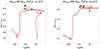 |
Fig. A.1. HR diagram for our GENEC evolution models, comparing new inner structure (Tayler-Spruit dynamo and Ledoux convective criterion, red solid lines) with old inner structure (no-TS dynamo and Schwarzchild convective criterion, dashed brown lines). |
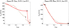 |
Fig. A.2. Rotational velocity during the MS for our GENEC evolution models, comparing new inner structure (Tayler-Spruit dynamo and Ledoux convective criterion, red solid lines) with old inner structure (no-TS dynamo and Schwarzchild convective criterion, dashed brown lines). |
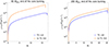 |
Fig. A.3. Specific angular momentum at the end of the He-core burning for our GENEC evolution models, comparing new inner structure (Tayler-Spruit dynamo and Ledoux convective criterion, blue) with old inner structure (no-TS dynamo and Schwarzchild convective criterion, orange). |
All Tables
Properties of our evolution models during the He-core and C-core burning stages.
Lifetime predicted by our GENEC and MESA models in the spectroscopic phases according to stellar evolution.
Table of final parameters for our GENEC models, comparing the new inner structure with the old inner structure.
All Figures
|
Fig. 1. HR diagram for GENEC (red) and MESA (blue) evolution models with 60 M⊙ (left panel) and 200 M⊙ (right panel). Black dots represent the point where Γe = 0.5 and thus the wind regime transits from thin to optically thick, black crosses represent the end of the H-core burning stage, black stars represent the beginning of the He-core burning stage, cyan stars represent the switch between H-rich to H-poor helium stars, and magenta stars represent the end of the He-core burning stage. |
| In the text | |
|
Fig. 2. Left panel: Evolution of mass-loss rate, stellar mass, stellar radius, and Eddington factor during the H-core burning stage for GENEC and MESA evolution models with Mzams = 60 M⊙. Right panel: Same as the left panel, but for evolution models with Mzams = 200 M⊙. |
| In the text | |
|
Fig. 3. Left panel: Evolution of mass-loss rate, stellar mass, stellar radius, and Eddington factor during the He-core and C-core burning stages for GENEC and MESA evolution models with Mzams = 60 M⊙. Right panel: Same as the left panel, but for evolution models with Mzams = 200 M⊙. |
| In the text | |
|
Fig. 4. Ṁ − Γe correlations taken from the GENEC self-consistent evolution models from Gormaz-Matamala et al. (2023) and this work. The dashed line represents the best linear fit for these Msc, whereas the gray dot-dashed line represents the fit of Eq. (5) adopted for Z = 0.014. |
| In the text | |
|
Fig. 5. η − Γe correlations taken from theoretical models tabulated by Krtička & Kubát (2017), Björklund et al. (2021), and Gormaz-Matamala et al. (2023). |
| In the text | |
|
Fig. 6. Distribution across the HRD of the evolutionary spectral types introduced in Sect. 4.3. The red and blue dots represents time intervals of 20 000 years, starting from the end of the H-core burning, for our GENEC and MESA models, respectively. |
| In the text | |
|
Fig. 7. Evolutionary GENEC and MESA tracks for 60 and 200 M⊙ from Fig. 1 and additional 100 M⊙ models, where the thick solid lines represent the segments where the wind is optically thick (Γe ≥ 0.5) and Xsurf ≥ 0.3. The gray stars correspond to the sample of WNh stars from Martins et al. (2008), the purple stars to the sample of Crowther et al. (2010) and the green stars to the sample of Hamann et al. (2019), tabulated in Table 4. Yellow shadowed area correspond to the HRD region where the HD limit is exceeded. |
| In the text | |
|
Fig. A.1. HR diagram for our GENEC evolution models, comparing new inner structure (Tayler-Spruit dynamo and Ledoux convective criterion, red solid lines) with old inner structure (no-TS dynamo and Schwarzchild convective criterion, dashed brown lines). |
| In the text | |
|
Fig. A.2. Rotational velocity during the MS for our GENEC evolution models, comparing new inner structure (Tayler-Spruit dynamo and Ledoux convective criterion, red solid lines) with old inner structure (no-TS dynamo and Schwarzchild convective criterion, dashed brown lines). |
| In the text | |
|
Fig. A.3. Specific angular momentum at the end of the He-core burning for our GENEC evolution models, comparing new inner structure (Tayler-Spruit dynamo and Ledoux convective criterion, blue) with old inner structure (no-TS dynamo and Schwarzchild convective criterion, orange). |
| In the text | |
Current usage metrics show cumulative count of Article Views (full-text article views including HTML views, PDF and ePub downloads, according to the available data) and Abstracts Views on Vision4Press platform.
Data correspond to usage on the plateform after 2015. The current usage metrics is available 48-96 hours after online publication and is updated daily on week days.
Initial download of the metrics may take a while.