| Issue |
A&A
Volume 697, May 2025
|
|
|---|---|---|
| Article Number | A193 | |
| Number of page(s) | 13 | |
| Section | Stellar structure and evolution | |
| DOI | https://doi.org/10.1051/0004-6361/202554078 | |
| Published online | 16 May 2025 | |
Exploring the connection between atmosphere models and evolution models of very massive stars
1
Zentrum für Astronomie der Universität Heidelberg, Astronomisches Rechen-Institut, Mönchhofstr. 12-14, 69120 Heidelberg, Germany
2
Department of Astronomy, University of Geneva, Chemin Pegasi 51, 1290 Versoix, Switzerland
3
Instituut voor Sterrenkunde, KU Leuven, Celestijnenlaan 200D, 3001 Leuven, Belgium
⋆ Corresponding author; This email address is being protected from spambots. You need JavaScript enabled to view it.
Received:
7
February
2025
Accepted:
10
April
2025
Abstract
Context. Very massive stars (VMSs) are stars that are born with masses of more than 100 M⊙. Despite their rarity, their dominance in the integrated light of young stellar populations and their strong stellar feedback make them worthwhile objects of study. Their evolution is dominated by mass loss, rather than interior processes, which underlines the significance of an accurate understanding of their atmosphere. Yet, current evolution models are required to make certain assumptions on the atmospheric physics which are fundamentally incompatible with the nature of VMS.
Aims. In this work, we aim to understand the physics of VMS atmospheres throughout their evolution by supplementing the structure models with detailed atmosphere models capable of capturing the physics of a radially expanding medium outside of local thermodynamic equilibrium. An important aspect is the computation of atmosphere models reaching into deeper layers of the star, notably including the iron-opacity peak as an important source of radiative driving. From this we investigate the importance of the seemingly arbitrary choice of the lower boundary radius of the atmosphere model.
Methods. We used the stellar evolution code GENEC to compute a grid of VMS models at solar metallicity for various masses. This grid implements a new prescription for the mass-loss rate of VMS. We then selected the 150 M⊙ track and computed atmosphere models at 16 snapshots along its main sequence using the stellar atmosphere code PoWR. For each snapshot, we computed two atmosphere models connected to the underlying evolutionary track at different depths (below and above the hot iron bump), sourcing all relevant stellar parameters from the evolutionary track itself.
Results. We present two spectroscopic evolutionary sequences for the 150 M⊙ track connected to an atmosphere model at different depths. Furthermore, we report on important aspects of the interior structure of the atmosphere from the perspective of atmosphere versus evolution models. Finally, we present a generalized method for the correction of the effective temperature in evolution models and compare it with results from our atmosphere models.
Conclusions. The different choice of connection between structure and atmosphere models has a severe influence on the predicted spectral appearance, which constitutes a previously unexplored source of uncertainty in quantitative spectroscopy. The simplified atmosphere treatment of current stellar structure codes likely leads to an overestimation of the spatial extension of VMSs, caused by opacity-induced subsurface inflation. This inflation does not occur in our deep atmosphere models, resulting in a discrepancy in predicted effective temperatures of up to 20 kK. Future improvements with turbulence and dynamically consistent models may resolve these discrepancies.
Key words: stars: atmospheres / stars: evolution / stars: massive / stars: winds, outflows
© The Authors 2025
 Open Access article, published by EDP Sciences, under the terms of the Creative Commons Attribution License (https://creativecommons.org/licenses/by/4.0), which permits unrestricted use, distribution, and reproduction in any medium, provided the original work is properly cited.
This article is published in open access under the Subscribe to Open model. This email address is being protected from spambots. You need JavaScript enabled to view it. to support open access publication.
1. Introduction
Massive stars (Mini ≳ 8 M⊙) are powerhouses in the Universe, driving the evolution of their host galaxies through extreme radiative, chemical, and mechanical feedback. Among them, very massive stars (VMSs, Mini ≳ 100 M⊙) are the most extreme specimen, shining millions of times brighter than their low-mass counterparts and producing mass-loss rates on the order of 10−4 M⊙/yr. Although initially predicted to be very rare by the initial mass function (IMF, Salpeter 1955), more recent evidence suggests that they are greater in number than expected (Schneider et al. 2018; Ramachandran et al. 2018; Vink 2018; Zeidler et al. 2017). Moreover, their powerful impact on their surroundings means that, despite their rarity, an accurate understanding of their physics is required for an accurate interpretation of the role of massive star populations as a whole (e.g., Crowther et al. 2016; Higgins et al. 2023; Upadhyaya et al. 2024).
In terms of evolution, VMSs are generally considered a small subcategory at the upper end of the massive star regime. However, there are several indicators that set VMSs apart from other massive stars, encouraging us to treat them as their own distinct class of star. Firstly, unlike other massive stars, most models suggest that VMSs lose enough mass while still on the main sequence (MS) to transition directly into the hydrogen-poor Wolf-Rayet (WR) regime before core hydrogen exhaustion, bypassing the blue and red supergiant phase of evolution (e.g., Ekström et al. 2012; Köhler et al. 2015; Gormaz-Matamala et al. 2025). Spectroscopically, most observed VMSs appear as WNh stars, morphologically extending from the early O-star regime (e.g., Crowther & Walborn 2011; Bestenlehner et al. 2014). VMSs are also potential progenitors of pair-instability supernovae (PISNe) and the still-elusive intermediate-mass black holes (Gabrielli et al. 2024; Spera & Mapelli 2017).
From a modeling perspective, VMSs still present significant challenges due to their complex physics. Stellar evolution models, which assume hydrostatic equilibrium and a simplified, optically thin atmosphere, are incompatible with the expanding atmospheres and strong winds expected and observed for VMSs. Consequently, the effective temperatures predicted from structure models and the resulting evolution in the Hertzsprung-Russell diagram (HRD) are questionable. Additionally, the evolution of VMSs is often modeled with mass-loss rates extrapolated from a lower-mass and lower-luminosity regime, introducing further uncertainties that then propagate through the entire evolution (Gräfener 2021; Josiek et al. 2024).
In this work, we aim to characterize the structure and appearance of VMSs through a combination of evolution models and detailed atmosphere models. This allows us to exploit the strengths of both modeling techniques and constitutes a first step toward understanding VMSs in a more physically consistent way. Furthermore, we investigate the robustness of this approach by exploring different boundary conditions between the atmosphere model and the underlying structure models along the evolutionary path.
The paper is laid out as follows. Sect. 2 introduces our evolution models and presents a new grid of VMS models with updated mass-loss rates. Sect. 3 presents our atmosphere models, detailing the methodology we use to post-process the evolutionary tracks with the atmosphere code. We then discuss the resulting spectroscopic evolution of VMSs in Sect. 4 and examine their atmospheric structure in Sect. 5. A summary of our findings is given in Sect. 6.
2. Stellar evolution models
2.1. Physical ingredients
In this work, we model VMSs using the Geneva stellar evolution code (GENEC, Eggenberger et al. 2008; Ekström et al. 2012). The basic input physics are equivalent to the ones used in the grid by Ekström et al. (2012), notably using abundances from Asplund et al. (2005) (except for Ne, which is from Cunha et al. 2006), and applying convection using a step-overshoot scheme with α = 0.1 with the Schwarzschild criterion. We implement the recent dedicated VMS mass-loss scheme from Sabhahit et al. (2022), which initially applies the standard mass-loss recipe for hot stars from Vink et al. (2001) and switches to an increased mass-loss rate as the star approaches the Eddington limit.
2.2. Calculated models
Figure 1 shows the grid of evolutionary tracks of our solar-metallicity, nonrotating VMS models computed with the updated mass-loss scheme in GENEC. All models were computed until the terminal-age main sequence (TAMS), which we define here as the moment when the central hydrogen mass fraction drops below 10−5.
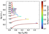 |
Fig. 1. Hertzsprung-Russell diagram showing the evolution of the nonrotating models of potential VMS computed with GENEC using the updated mass-loss scheme. Each track is labeled with the corresponding initial mass (in M⊙). The red and blue markers represent the ZAMS and TAMS, respectively. The color of the tracks indicates the surface hydrogen content across the evolution. |
As a prototype of VMS evolution, we now focus specifically on the 150 M⊙ model. According to typical evolutionary (i.e., non-spectroscopic) surface abundance criteria, this star is expected to evolve from O to WR type while still on the MS (e.g., Yusof et al. 2013; Josiek et al. 2024), allowing us to study the WR transition while avoiding uncertainties associated with post-MS evolution. Fig. 2 shows the MS track of the nonrotating 150 M⊙ model from our grid, as well as a model initially rotating at 0.1vcrit computed with the same mass-loss prescription for comparison.
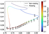 |
Fig. 2. Hertzsprung-Russell diagram showing the evolution of the 150 M⊙ models computed with GENEC using the new mass-loss scheme. The initial velocity of the rotating model was set at 10% of the critical velocity. The markers (labeled 00−15) represent the evolution snapshots used to compute atmosphere models with PoWR along the nonrotating track. The color of the tracks indicates the evolving surface hydrogen content of the models. |
The rotating model inflates much less along the MS than the nonrotating one, despite having a larger core-to-envelope ratio. The inflation taking place for these models on the MS is mainly caused by an opacity effect close to the surface. The rotating model, having more efficient mixing, evolves almost chemically homogeneously with a significantly higher surface helium mass fraction than the nonrotating model. Because of this, the Thompson scattering opacity in the atmosphere is reduced and there is less inflation.
Figure 3 underlines that the entire apparent inflation of the nonrotating model during the MS takes place above an optical depth of τ ≈ 1000, being mainly driven by the subsurface iron opacity peak. Importantly, this implies that predictions of observables such as effective temperature and spectral features during this phase rely on the accuracy of the atmosphere physics assumed at the very surface of the structure model. The main uncertainty herein lies in distinguishing between inflation and wind launching, for which evolutionary codes must make an ad hoc assumption since the wind is not included in the structure models. To gain a deeper understanding of this regime, we therefore calculate dedicated atmosphere models smoothly connected to the deeper stellar structure in this work.
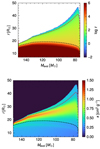 |
Fig. 3. Evolution of the interior atmospheric structure of the continuum optical depth (top) and the total Rosseland mean opacity (bottom) of a nonrotating 150 M⊙ star during the MS. The dashed red line shows the location of τ = 20, and the dashed black line marks a local density of 10−7 g cm−3. These represent the connection boundary for the atmosphere models outlined in Sect. 3.2. |
Finally, we note that the MS inflation taking place here is fundamentally different from the expansion that a star experiences at the end of the MS, which is driven from much deeper inside the star (the convective core boundary lies at τ ∼ 1010). In this regard, Sabhahit & Vink (2024) distinguish between the terms “inflation” and “expansion”, the former of which is used to describe the surface phenomenon discussed here. For consistency, we follow the same distinction throughout this paper.
3. Atmosphere models
3.1. The atmosphere in stellar evolution models
Stellar evolution codes were originally not designed to treat stars with extended expanding atmospheres, such as VMS. Moreover, due to a lack of hydrostatic equilibrium and very complex radiative transfer, realistic models for expanding atmospheres are numerically expensive on their own. Consequently, the surface boundary conditions in evolutionary codes are usually kept rather simple with very important atmosphere physics missing from the models. In GENEC, the upper layers of the star (representing between 1−2% of the stellar mass) are counted as the so-called “envelope”. In this region, the stellar structure is integrated hydrostatically over the density (instead of the pressure) in order to improve numerical stability and avoid density inversions1.
At the top of the envelope, a gray atmosphere is appended as a boundary condition. The atmosphere stratification is then computed over the optical depth with  , where Teff is the temperature of the layer immediately below the atmosphere, which is fixed at
  .
.
Notably, no wind is included in the structure of the atmosphere. However, Langer (1989) derived a method of estimating a correction on the effective temperature based on a wind attached to the upper boundary of the stellar model. This method assumes a β velocity law with β = 2 for the wind (see also Sect. 3.2) and computes the correction on the photospheric radius R2/3 due to the additional optical depth of the wind as follows:
 (1)
(1)
where κ is the (density-independent) opacity of the wind,  is the mass-loss rate, and v∞ is the terminal wind velocity. R is the surface radius of the stellar structure model. The calculated R2/3 is then the radius at which the wind reaches an optical depth of 2/3. From this, the corrected effective temperature is obtained via the Stefan-Boltzmann relation. The opacity, κ in Eq. (1) should ideally be the flux-weighted mean opacity. However, as this cannot be determined from the structure models, it is either simply approximated by the electron-scattering opacity, σe (e.g. in optical depth estimations such as in Langer 1989; Szécsi et al. 2015; Aguilera-Dena et al. 2022), or – as was described in more detail in Schaller et al. (1992) – by a force multiplier approach, κ = σe(1 + ℳ), with ℳ following from a modified CAK (after Castor et al. 1975) solution, namely the famous “cooking recipe” by Kudritzki et al. (1989). The latter has become the standard in GENEC for the wind-corrected temperatures reported in the WR stage since Schaller et al. (1992). Despite its level of sophistication, this “wind correction” requires not only the assumption of β but also the choice of force multiplier parameters, which in the case of the GENEC application were taken from the 50 kK model in Pauldrach et al. (1986).
In Groh et al. (2014), these wind-corrected effective temperatures (for β = 2 and the other assumptions) were compared to Teff values resulting from CMFGEN calculations for an evolutionary track of a star with an initial mass of 60 M⊙. Generally, the GENEC-inherent corrections were found to be too strong with the specific differences being more complex than a simple scaling factor. Still, the basic concepts of the described procedure could prove useful when estimating effective temperatures of evolution models with significant winds. In Sect. 5.5, we generalize it to any β as well as the case of optically thin winds (R2/3 < R), and we compare the resulting approximation to results from detailed atmosphere models.
3.2. Structure computation in detailed atmosphere models
In this work, we have used the Potsdam WR code (PoWR, Gräfener et al. 2002; Hamann & Gräfener 2003; Sander et al. 2015) to compute detailed models of the stellar atmosphere along a computed evolutionary track. PoWR models a spherically expanding non-LTE atmosphere in 1D, performing a detailed radiative transfer in the comoving frame (CMF).
The structure of a stellar atmosphere within our framework is defined by a single function, either the density ρ(r) or velocity v(r), as the two are connected by the continuity equation
 (2)
(2)
In principle, the velocity structure in a 1D stationary atmosphere could be obtained consistently from solving the hydrodynamic equation of motion (e.g., Gräfener & Hamann 2005; Sander et al. 2017; Sundqvist et al. 2019). However, coupled with a detailed non-LTE and CMF calculation, this is numerically very costly. While we shall explore this approach for selected snapshots in a future paper – based on the insights gained in this work – an important first step is to connect structure and atmosphere models in a well-described manner using standard atmosphere modeling. In contrast to dynamically consistent model calculations, this approach could later also be scaled to a larger parameter range.
In the standard approach, the structure is split radially into two domains. In the lower domain, we assume the kinetic acceleration, v ∂v/∂r, to be small compared to gravity, allowing us to neglect this term and assume hydrostatic equilibrium instead (see Sander et al. 2015, for the implementation in PoWR). This domain is then smoothly connected to the wind domain, for which we assume the velocity to follow a so-called beta-law:
 (3)
(3)
where v∞ and β are free parameters and p is determined by the connection settings between the two domains. Two options for this connection are available in PoWR: either, the wind velocity profile connects with a smooth gradient to the hydrostatic regime, or the connection is forced at a specific fraction of the sound speed. For the terminal velocity v∞, we chose 2.65 times the escape velocity at the photosphere, as was suggested by (modified) CAK results (Kudritzki & Puls 2000). Motivated by hydrodynamically-consistent models of WNh atmospheres by Gräfener & Hamann (2008), we chose β = 1 (see also Fig. 2 in Hamann et al. 2008).
Our framework for the atmosphere models implies that the effective temperature at  , denoted simply as Teff, is no longer a boundary condition as in the evolutionary code, but is instead calculated intrinsically given the converged atmosphere and wind structure. As a result, Teff can diverge significantly between different modeling methods given the same underlying stellar parameters.
3.3. Grid setup
Along the nonrotating 150 M⊙ evolutionary track calculated with GENEC, we selected 16 snapshots of the stellar structure along the MS for which to compute detailed atmosphere models using PoWR. These points, marked ‘00’ (ZAMS) to ‘15’ in Fig. 2, are separated by a mass loss of about 5 M⊙ between them, which results in roughly even intervals in the HRD. The nonrotating track was selected (vs. the rotating one) for its notable inflation along the MS, a phenomenon we wanted to investigate further using our detailed atmosphere models. In order to explore the connection between the structure and atmosphere models as well as probe the effect of including the iron opacity peak within the atmosphere boundaries, we computed two models at each point with different connection depths.
In PoWR, the depth of the atmosphere is usually set via the parameter TAUMAX, which represents the Rosseland mean optical depth, without the contribution of line opacities, of the deepest radial point. This, together with the inner radius, RSTAR, defines the lower boundary of the PoWR stratification. While the continuum optical depth is not a quantity directly available in stellar structure models, we can estimate it using Kramer’s opacity law and extract the corresponding radial coordinate, RSTAR from the GENEC structure. First, we computed a series of models with a relatively shallow optical depth of TAUMAX=20, which represents the “standard” way of computing atmosphere models. It is similar to the approach used by Schaerer et al. (1996a,b), Groh et al. (2014), and Martins & Palacios (2022). The latter can also serve as a comparison point for our results.
Alternatively to a connection based on optical depth, we can also define the lower boundary by its radial velocity, vmin. This enables us to connect the atmosphere structure continuously to the interior structure models at a specific density via the continuity equation. For the deep models, we chose the boundary as the radius at the density ρ = 10−7 g cm−3, which is beneath the entire super-Eddington hot iron bump region. In comparison to the shallow models, the continuum optical depth of this point is on the order of ∼1000.
The stellar parameters extracted from GENEC are shown in Table 1. In addition to the abundances shown in this table for H, C, N, O and Ne, we include the elements S, Si, and Ar, whose surface abundances we assumed to be constant during the evolution and which we obtained from Asplund et al. (2009)2. The elements from Sc to Ni (the “iron-group”) are combined in PoWR into a single generic element, “G”, in a super-level approach (Gräfener et al. 2002). Finally, the abundance of He is not an explicit input of the model but is instead calculated as the missing fraction from all the included elements.
Variable input parameters of the PoWR models along the evolutionary tracks of the nonrotating 150 M⊙ models.
For grid points 11 to 15, representing the last 0.4 Myr of MS evolution, the shallow modeling procedure did not produce a converged output. This is most likely due to the fact that the lower boundary of these models is beyond the Eddington limit, violating the requirement of hydrostatic equilibrium in the inner part. Furthermore, non-convergence could be a sign that the underlying (inflated) structure computed in GENEC has become so unphysical that it yields unrealistic stellar parameters, which are then used as inputs for PoWR.
4. Spectroscopic analysis of the PoWR models
4.1. Analysis of the evolutionary sequence of models
Figure 4 shows the evolution of the normalized optical spectra computed for the deep and shallow sequence in PoWR. The ZAMS spectra (darkest blue) show very little difference between the two connection depths, with both models exhibiting mainly absorption features typical of O stars, as well as a weak He II 4686 emission line. For the first four grid points, the spectra from both sequences look qualitatively very similar.
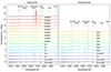 |
Fig. 4. Optical spectrum for deep (left) vs. shallow (right) models across evolution (from bottom to top). The spectra are vertically offset so that the continuum level corresponds to the grid point number on the y axis for easy reading. The spectral types were estimated based on the classification scheme in Crowther & Walborn (2011). |
After grid point 03 (between 0.85 and 1.04 Myr), there appears to be a switch in the spectral type of the shallow models, with several lines going into emission, notably Hβ and Hγ among the other Balmer lines, as well as the N IV 4058 line, classifying the model as WNh-type. The emission lines become more prominent with time until reaching a peak at grid point 06, after which they begin to recede slightly, while still remaining stronger than the ones in the corresponding deep models. Such an evolution is consistent with spectra predicted using a similar method by Martins & Palacios (2022) for VMSs. Interestingly, this behavior is completely absent in the deep model series, according to which we could classify this 150 M⊙ star as O-type or at most O/WNh for its entire MS evolution, with the spectrum changing much more gradually.
While the hydrogen and nitrogen lines go into emission after the switch in the shallow models, the He II lines remain in absorption (with the exception of He II 4686, whose emission increases considerably). Therefore, the spectral transition from O to WR type seems to be related only to the behavior of hydrogen in the atmosphere. To test this, we repeated the computation of the shallow grid point 04 spectrum while switching off the contribution of all Hydrogen lines. Indeed, this yields a qualitatively similar output to the ZAMS models. It turns out that the appearance of hydrogen emission lines in the VMS is related to a switch in the ionization stratification of hydrogen in the star, which we discuss more in Sect. 5.
Interestingly, the transition from O to WR spectra in the shallow models series occurs much sooner than assumed in evolutionary codes, in which a surface hydrogen mass fraction of 0.3 is typically taken as the transition criterion. If the shallow models are to be believed, this suggests that a different criterion would be better suited for defining the beginning of the WR phase in evolution models for VMSs.
Finally, we also inspected the spectrum in the UV range, shown in Fig. A.1. Although there are some differences between the deep and shallow model series, they are much less striking than the ones discussed for the optical spectrum.
4.2. Potential discrepancy in mass-loss diagnostics
Both the shallow and the deep model formally have the same mass-loss rates, despite their spectral differences. In turn, this raises the question of whether the choice of inner boundary in a model atmosphere could affect the derived mass-loss rates in quantitative spectroscopy. To test this, we now assume that the deep model represents an observation that we would routinely fit with a shallow model, as those represent the typical atmosphere calculation assumptions.
We carried out this experiment for grid point 06, where we visually identified the greatest difference in the two spectra (see Fig. 4). For this point, we took the existing shallow model as a baseline and then varied only the mass-loss rate until we obtained a model, the spectrum of which was close to that of the deep model at the same grid point. For simplicity, we fixed the other input parameters during this procedure. While this would not be the case in an actual quantitative spectroscopic analysis, our main aim is to determine whether there is a systematic difference in the derived  .
.
Figure 5 shows the spectra from the shallow and deep models as well as several adjusted versions of the shallow model with different mass-loss rates. We focus on the wavelength range around the He II 4686 and Hβ emission lines, since these tend to be strongly affected by the wind. For the inspected grid point, we see that reducing the mass-loss rate from the prescribed −4.513 to −4.7 results in the helium line matching the deep model’s spectrum very closely. This reduction in  also results in the weakening of the Hβ emission line, but it does not yet reach the stronger absorption seen for the deep model. The models with
  and
and  produce a closer fit to the Hβ line.
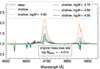 |
Fig. 5. Fitting of the deep model spectrum with a shallow model of varying mass-loss rates at grid point 06. The original prescribed mass-loss rate used for the main models (green and yellow) and the evolutionary track is given in the boxed text for comparison. |
This simple modeling experiment reveals a possible uncertainty in the mass-loss rate determination of up to 0.4 dex, caused just by the connection of atmosphere models to evolution models. Ultimately, this underscores the still uncertain physics of VMSs as it is implemented into structure and atmosphere models. If the deep atmosphere models were representative of the nature of VMS, this would imply that current fitting methods routinely underestimate the mass-loss rates of such stars.
5. Structure comparison
5.1. Density profile
Figure 6 shows the density profiles of the GENEC model and both atmosphere models across the evolution of our example star. The evolution of the density profile of the GENEC models shows the establishment of a wide density plateau as a result of MS inflation (see also Fig. 3). By design, the deep PoWR model connects below this density plateau and the shallow model connects above it. As opposed to the GENEC models, the deep PoWR model does not include an inflated region. As a result, the density profiles of both atmosphere models differ increasingly over the evolution. However, although different in the inner part, the different density structures of the atmosphere models reconcile in the wind, past x ≈ 0.5 (r ≈ 2 Rdeep).
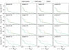 |
Fig. 6. Density stratification across the MS evolution of the two PoWR model series compared to the GENEC structure models. The grid points correspond to the locations shown on the HRD in Fig. 2. The x axis represents the modified radial coordinate 1 − Rdeep/r, where Rdeep is the lower boundary radius R* of the deep model. This scaling allows us to visualize both the inner part and the wind domain of the atmosphere (see, e.g., figures in González-Torà et al. 2025; Debnath et al. 2024). |
We also note that the density profiles of both PoWR models connect continuously to the GENEC model. For the deep models, this follows from tying their lower boundary directly to the GENEC density profile at ρ = 10−7 g cm−3. For the shallow models, the density continuity indicates that our approximation of the continuum optical depth in GENEC is reasonable for the upper layers of the atmosphere.
Given the differences between the obtained curves, it is a priory not clear which of the approaches marks the best representation of a VMS atmosphere. The limitation to 1D enforces approximations of the effect of the (hot) iron opacity peak, which differ between the structure and atmosphere model.
In GENEC, the model is assumed to be quasi-static instead of strictly static, meaning that the star is allowed to evolve on thermal timescales. As a result, hydrostatic equilibrium can still be found by allowing excess radiative energy to be converted to kinetic energy in the envelope, which ultimately causes the star to inflate. This inflation is a common effect in evolution models of stars close to the Eddington limit, where it also depends on the convection scheme applied in the subsurface region (Köhler et al. 2015; Gräfener 2021).
In contrast, the (quasi-)hydrostatic regime beneath the wind in stellar atmosphere codes does not allow for any super-Eddington layer. The codes therefore either do not cover this regime and only model the wind or need to make an arbitrary cut in the radiative acceleration exceeding the Eddington limit. Following the tradition of TLUSTY (e.g., Hubeny & Lanz 1995), the default cutoff in PoWR has long been at Γrad = 0.9, but recently increased to 0.99. Any additional radiative acceleration is simply ignored, leading to a relatively compact atmosphere with a spectrum dominated by absorption lines. A priori, the evolution model may seem more physically plausible as it does not include an arbitrary cutoff of the Eddington parameter. However, this model also does not account for other effects that may play an important role related to the iron bump.
One possibility is to launch an optically thick wind already from the iron bump itself. If the star is close enough to the Eddington limit, acceleration over the iron bump can be sufficient to launch a supersonic flow also below the photosphere. This happens for example in a significant number of classical WR stars (e.g., Gräfener & Hamann 2005; Sander et al. 2020; Poniatowski et al. 2021). In multiple dimensions, the redistribution of the gas into clumps with relatively high densities and channels with relatively low densities can artificially increase the effective driving in the atmosphere (Moens et al. 2022). This would mean that there is already a significant radial velocity field also underneath the photosphere that is not covered in a hydrostatic approach and as such would strongly alter the atmosphere and wind physics. One direct effect of these altered physics is that the outflow will not follow the typically assumed β-velocity law. On the other hand, spectroscopic evidence suggests that launching a wind at the iron bump is not likely for VMSs, given that wind lines would then appear much stronger than observed (see, e.g., the spectra in Sander et al. 2023, arising from deep-wind launching).
Alternatively, if the star does not manage to maintain an outflow, multidimensional models show that the atmosphere can fragment and partially fall down back on the star (sometimes known as a “failed wind”). This suggests that the strong inflation seen in 1D models due to the effective scale height approaching infinity (Langer et al. 2015) is actually unstable and an artifact of the current 1D model limitations combined with the forced hydrostatic equilibrium. In the case of a failed wind, the iron bump can trigger radiatively driven turbulent motion (Moens et al. 2022; Debnath et al. 2024). This turbulence is initiated by a gas parcel being driven upward by increased opacity, expanding and therefore decreasing its opacity, causing it to fall back down. From current 3D model calculations, this effect is not expected to contribute much to the energy transport in the upper layers of hot stars, but could significantly affect its structure through the introduction of additional turbulent pressure. The turbulent pressure alters the total pressure scale height, which locally softens the temperature and density profiles. Some results from 2D hydrodynamical models indeed support the absence of a density plateau (or in more extreme cases an inversion), similar to our deep models (Debnath et al. 2024). In this case, our deep model sequence would represent a more realistic view of what VMSs actually look like, which throws into question the interpretation of previous observations.
Recent 1D approximations of O-star atmosphere calculations (González-Torà et al. 2025) including a constant turbulent pressure show that even the density drop further inward observed in our deep models might be washed out by turbulent motions. Therefore, it is likely that the density profiles of our two modeling approaches in PoWR represent two extreme possibilities for the atmospheric structure of VMSs. Including a more sophisticated – non-radially constant – treatment of turbulent pressure in the 1D code should then result in a more gradual density decrease than our deep models, while not being as inflated as what is suggested by GENEC and the attached shallow model. Extending the implementation of turbulence and exploiting the code’s full hydrodynamic capabilities is beyond the scope of the present paper, but will be explored in a future work.
5.2. Temperature profile
Figure 7 shows the evolution of the temperature profile of the GENEC model with the deep and shallow atmosphere model. For the PoWR models, the curves represent the electron temperature as there is no general temperature in a non-LTE regime. In the deep layers of the atmosphere, LTE is recovered and the electron temperature is thus identical to the gas temperature.
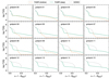 |
Fig. 7. Temperature stratification across the MS evolution of the two PoWR model series as well as the GENEC structure models. The grid points correspond to the locations shown on the HRD in Fig. 2. For the PoWR models, the electron temperature is shown. |
First, we note that the respective temperature connection between both atmosphere models and the structure model is excellent throughout the evolution. This is expected since the diffusion approximation is assumed to be valid at the lower boundary of the models, causing the electron temperature to coincide with the LTE temperature of the GENEC models at that point.
The qualitative temperature profile of the deep models remains very similar throughout the entire MS evolution. There is a sharp drop in the temperature until about x ≈ 0.1 (r ≈ 1.1 Rdeep) at ∼40−50 kK, after which the temperature decrease enters a more gradual regime. The transition point is optically very close to the surface of the star, at τRoss = 0.01, and thus its spectrum is mostly formed in the region with the steep temperature gradient.
The shallow models follow a similar temperature profile as the deep models for the first four grid points. At grid point 04 the temperature decrease in the inner part suddenly starts to extend much deeper, reaching the minimum of 8000 K imposed by PoWR after less than one stellar radius. This transition, coinciding with the spectral O→WR transition (see Fig. 4), is closely related to the recombination of hydrogen in the wind, which we show in Fig. 8. As the evolution model inflates during the MS, the shallow PoWR models (which follow this inflation) are attached at an increasing radius and therefore have a decreasing lower boundary temperature. Eventually, this causes the recombination of H II to H I in the atmosphere, which provides additional cooling leading to a further temperature decrease. This effect is a positive feedback loop, triggered by the crossing of some temperature threshold, which explains the very sudden change in temperature and ionization structure of the wind between just two grid points, representing an upper limit on the transition time span of just 190 kyr.
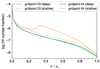 |
Fig. 8. Stratification of the neutral hydrogen number fraction for the models at grid points 03 and 04 for the 150 M⊙ track, showing the appearance of a recombination region for the shallow models at grid point 04. The subsequent shallow models in the series look qualitatively similar to the grid point 04 shallow model shown here, whereas no prominent recombination peak appears for any of the deep models. |
Conversely, despite having the same mass-loss rate as shallow models, the temperature profile of the deep models keeps a very similar shape throughout the series with no further abrupt drops. For the same density, the temperature in the shallow models is much lower than in the deep ones. This could be a further sign that the inner boundary of the shallow models is not deep enough and some of the assumptions there are invalid. As a consequence, the temperature correction algorithm likely overpredicts the cooling in the wind of the shallow models.
5.3. Opacity profile
Figure 9 shows the opacity profile of the deep and shallow PoWR models and the GENEC structure models over the course of the MS evolution of our 150 M⊙ VMS. For the GENEC models, the opacity is the Rosseland mean opacity obtained from tabulated values for a solar-mixture gas interpolated for metallicity, temperature and density. In PoWR, we obtain both the calculated Rosseland mean opacity given the conditions of the gas and the provided atomic data, as well as the flux-weighted mean opacity. As the name suggests, the latter is dependent on the spectral flux distribution and is directly related to the radiative acceleration via
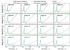 |
Fig. 9. Evolution of the atmospheric profile of the Rosseland and flux-weighted mean opacities of the PoWR models, as well as the tabulated Rosseland mean opacity of the GENEC models. The opacity threshold for which the radiative acceleration surpasses gravity, as calculated by Eq. (5), is also shown. |
 (4)
(4)
As such, we can also calculate the opacity corresponding to the Eddington limit from the condition arad = g, which yields a constant only dependent on the current luminosity-to-mass ratio:
 (5)
(5)
The Rosseland mean opacity corresponds to the flux-weighted mean opacity in the case of a blackbody spectrum (LTE), an approximation that is valid in the deeper layers of the star. In the wind, Fig. 9 clearly shows a departure from LTE as the flux-weighted mean opacity becomes significantly super-Eddington, whereas the Rosseland mean opacity remains below the Eddington limit. In the deep PoWR models, this departure occurs above the super-Eddington iron bump region. In stellar structure models, which lack the detailed radiative transfer needed to simulate a spectrum, the flux-weighted mean opacity (and thus the radiative acceleration) cannot be obtained intrinsically, rendering it impossible to self-consistently predict the launching of any line-driven stellar wind3.
The profile of the Rosseland mean-opacity looks qualitatively similar throughout the MS evolution for both PoWR and GENEC models. The deep PoWR model in particular shows hardly any evolution in the opacity structure, with the location and shape of the hot iron bump remaining virtually unchanged. The iron bump itself has a noticeably higher maximum opacity in the PoWR model than is predicted by the tabulated opacities in GENEC, in part due to the assumed Doppler broadening of lines in PoWR. For all models, the entire opacity profile shifts downward slightly as the hydrogen mass fraction drops, reducing the contribution of Thompson scattering to the opacity. However, the Eddington limit decreases still faster due to strong mass loss and increasing luminosity, resulting in a stronger wind. For the later grid points, even the lower boundary of the deep PoWR models is already in the super-Eddington regime, in contrast to the GENEC models. In addition the opacity in GENEC is smeared out to larger radii as the atmosphere inflates, as is also shown in Fig. 3.
In the wind regime, both PoWR models show a very similar opacity profile for the first grid points. For the later grid points, the flux-weighted opacity of the shallow models increases more steeply in the wind than the ones of the deep models. This is a consequence of the recombination in the shallow models, which not only contributes hydrogen bound-free opacity, but also line opacity due to the recombination of other elements, especially iron.
5.4. Effective temperature in evolution versus atmosphere models
The effective temperature, Teff, is a fundamental parameter of a massive star that plays a multifaceted role in the star’s modeling. In evolutionary codes, it is computed as a boundary condition necessary to solve the stellar structure equations and then provided as an output. Additionally, the value of Teff feeds back into the evolution itself through its role in the computation of the mass-loss rate, which has important repercussions for many aspects of the evolution. Therefore, accurately modeling the effective temperature is not only important for the prediction of a star’s location in the HRD, but also to constrain the nature of the evolution itself.
The effective temperature computed by GENEC is simultaneously the temperature at the surface of the structure model, which is a boundary condition specifically determined to obtain a valid solution of the stellar structure equations in the interior. By design, a gray atmosphere with an optical depth of exactly 2/3 is appended to the structure model, resulting in the photosphere always coinciding with the surface of the hydrostatic star. However, this is not a physical necessity, and is in fact not true in stars with strong winds that completely obscure the hydrostatic layers.
In PoWR models, we refer to the effective temperature at τ = 2/3 as T2/3. We note that this does not necessarily correspond to the electron or flux temperature at this layer, since the atmosphere is generally outside of LTE. Nonetheless, T2/3 is physically most similar to the meaning of the effective temperature in evolutionary codes, which is why we chose this value as the point of comparison. We present the resulting effective temperatures from the different models in Table 2. The results are plotted in Fig. 10. It is evident that the deep models yield systematically higher effective temperatures, despite having the same mass-loss rates. This difference grows as the Teff is predicted to decrease by GENEC (because of inflation), whereas it stays comparatively constant in the deep PoWR models.
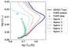 |
Fig. 10. Evolution of the 150 M⊙ star on the HRD using different methods to obtain the effective photospheric temperature T2/3. The solid black line shows the unmodified output of the GENEC track, and the square and circle scatter points show the output of the PoWR deep and shallow model series along the evolutionary track. The five nonsolid lines follow the approximated wind-corrected photospheric temperature calculated from the GENEC structure models via the method outlined in Sect. 5.5 using different assumptions for the connection radius Rcon (see main text for details). |
Output of effective photospheric temperature of the different models in kilokelvins.
5.5. A general correction method for the effective temperature in evolution models with wind
Starting from a computed structure model, we can cut off some upper layers and attach a simple wind regime to obtain a correction on the photospheric radius (and thus, temperature). Assuming a β velocity law, this correction can be derived analytically based on simple approximations. We outline this method here. It constitutes a generalization of the wind correction derived by Langer (1989) for optically thick winds with β = 2.
First, we choose some radius, Rcon, at which the wind connects to the hydrostatic regime. This choice is arbitrary and constitutes the only free parameter of this method. It can be chosen in a physically motivated way, and we implemented this method for different examples. The velocity law is then assumed to be
 (6)
(6)
where R0 is a theoretical radius where the velocity law reaches 0. Since continuity requires a strictly positive velocity, the connection point must be above the zero point; that is, Rcon > R0. Given a chosen Rcon, R0 can be determined from the continuity equation as
 (7)
(7)
where ρ(Rcon) is the density at the connection radius, which can be extracted from the stellar structure model. The wind parameters,  and v∞, are the result of prescriptions.
The optical depth in the wind (i.e., for r > Rcon) as a function of radius can then be computed as an integral over opacity:
 (8)
(8)
Using the continuity equation (Eq. 2) to replace the density, inserting the velocity law (Eq. 6), and assuming a constant (Rosseland-mean) opacity, κ, in the wind yields
 (9)
(9)
which can be evaluated analytically to obtain
 (10)
(10)
or in the case β = 1:
 (11)
(11)
Now, we can determine if this simple wind model is optically thick with the condition
 (12)
(12)
If this condition holds, then the photospheric radius is inside the wind and can be determined by simply inverting Eqs. (10) and (11) for τ(r) and setting τ = 2/3. This yields
 (13)
(13)
and for β = 1:
 (14)
(14)
If Eq. (12) does not hold, then the wind is optically thin. In order to find the photospheric radius, we must then integrate the structure model below the connection point as follows:
 (15)
(15)
The photospheric radius, R2/3, can then determined by inverting this equation numerically and setting τ = 2/3.
Finally, the corrected effective photospheric temperature can then be calculated as
 (16)
(16)
Using the described method, we can now determine a correction on the effective photospheric temperature computed by the evolutionary code and compare it with the output of the detailed atmosphere models computed by PoWR. Since the choice of connection radius, Rcon, remains a free parameter in the correction method, we show the results using different choices for this radius as examples:
-
(1)
Connection at the point at which the velocity (computed via the continuity equation) reaches 20% of the isothermal sound speed
 .
. -
(2)
Connection at the maximum of the Rosseland mean opacity in the hot iron bump.
-
(3)
Connection above the super-Eddington iron bump, where ΓEdd falls below unity.
-
(4)
Connection at the surface radius determined by GENEC.
-
(5)
Connection at a Rosseland mean optical depth of 1000.
We show the resulting tracks alongside the output of the PoWR models in Fig. 10. It is clear that all correction methods yield a similarly shaped evolutionary track that is shifted toward the hot side of the HRD by differing amounts. Notably, none of the explored approximations can reproduce the track of the deep PoWR model series. While approximation (5) comes closest to these points, it still underestimates the effective temperature by up to 5 kK in the second half of the MS. The mismatch between the GENEC approximations and the PoWR models is likely not only caused by the uncertainties of the approximation method itself, but also by the inconsistent treatment of the hydrostatic domain in PoWR causing differences between the two codes already below the wind. In the future, when hydrodynamically consistent series of PoWR models using more realistic physics exist as a point of comparison, this approximation method can be revisited to determine quick and reliable wind corrections from evolution models.
6. Summary and conclusion
In this work, we present two sequences of detailed atmosphere models computed in PoWR along an evolutionary track of a 150 M⊙ VMS computed with GENEC. The two model sequences differ in their connection depth to the underlying structure models, allowing us to investigate the impact of this choice of boundary condition. The shallow models use a traditional approach, connecting at a continuum optical depth of 20. For VMS evolution models, this is above a region experiencing significant opacity-induced inflation. Our deep atmosphere models use a new connection approach, employing a fixed density to connect to the structure models below this inflated region, representing the first such atmosphere models computed for VMSs.
Our results show significant differences between the deep and shallow models in terms of spectral lines and atmospheric structure. Because PoWR suppresses super-Eddington opacities in the hydrostatic layers, no inflated region is established in the deep models, as most of the radiative force generated in the hot iron bump is ignored. Spectroscopically, this results in much more absorption-line-dominated spectra typical of O stars. Conversely, the shallow model spectra show a rapid transition from O-type to emission-dominated WNh-type spectra after around 1 Myr of evolution, as was previously expected of VMSs. These differences in spectra between the two series arise despite all stellar parameters being identical, revealing previously unexplored systematic uncertainties in quantitative spectroscopy. For the mass-loss rate, we estimate a possible error of up to 0.4 dex (a factor of 2.5) arising from the choice of model depth.
The deep and shallow models differ significantly in the deduced effective temperatures. The shallow models closely resemble the temperatures predicted by GENEC, while the deep models are up to 20 kK hotter. No simple correction formalism can fully account for this so far. In their current state, neither the evolutionary code nor our PoWR models (deep and shallow) are able to fully capture all of the relevant physics in the atmospheres of VMS. Insights from multidimensional atmosphere models have identified turbulent motion driven by the iron opacity peak as one such physical ingredient that has yet to be implemented consistently into 1D codes. We expect that a future introduction of turbulence in the atmosphere models and the usage of dynamically consistent atmosphere models will result in a solution in between our deep and shallow models.
This actually marks one of the GENEC specifics as such density inversions are common results in other hydrostatic structure models (see, e.g., Ishii et al. 1999; Gräfener et al. 2012; Sanyal et al. 2015).
The exact mass fractions were retrieved from this table: http://astro.uni-tuebingen.de/~rauch/TMAP/TMAP_solar_abundances.html
A potential exception could be winds launched by the (hot) iron bump, where line opacities not yet broadened by a wind velocity field are decisive. Moreover, flux-weighted opacity tables such as the ones from Poniatowski et al. (2022) might become a future option.
Acknowledgments
We would like to thank our referee whose comments helped us improve the quality of this manuscript. JJ acknowledges funding from the Deutsche Forschungsgemeinschaft (DFG, German Research Foundation) Project-ID 496854903 (SA4064/2-1, PI Sander). AACS, MBP, RRL, and VR are supported by the Deutsche Forschungsgemeinschaft (DFG – German Research Foundation) in the form of an Emmy Noether Research Group – Project-ID 445674056 (SA4064/1-1, PI Sander). GGT acknowledges financial support by the Federal Ministry for Economic Affairs and Climate Action (BMWK) via the German Aerospace Center (Deutsches Zentrum für Luft- und Raumfahrt, DLR) grant 50 OR 2503 (PI: Sander). NM acknowledges the support of the European Research Council (ERC) Horizon Europe grant under grant agreement number 101044048. ECS acknowledges financial support by the Federal Ministry for Economic Affairs and Climate Action (BMWK) via the German Aerospace Center (Deutsches Zentrum für Luft- und Raumfahrt, DLR) grant 50 OR 2306 (PI: Ramachandran/Sander). JJ, MBP, RRL, and ECS are members of the International Max Planck Research School for Astronomy and Cosmic Physics at the University of Heidelberg (IMPRS-HD).
References
- Aguilera-Dena, D. R., Langer, N., Antoniadis, J., et al. 2022, A&A, 661, A60 [NASA ADS] [CrossRef] [EDP Sciences] [Google Scholar]
- Asplund, M., Grevesse, N., & Sauval, A. J. 2005, ASP Conf. Ser., 336, 25 [Google Scholar]
- Asplund, M., Grevesse, N., Sauval, A. J., & Scott, P. 2009, ARA&A, 47, 481 [NASA ADS] [CrossRef] [Google Scholar]
- Bestenlehner, J. M., Gräfener, G., Vink, J. S., et al. 2014, A&A, 570, A38 [NASA ADS] [CrossRef] [EDP Sciences] [Google Scholar]
- Castor, J. I., Abbott, D. C., & Klein, R. I. 1975, ApJ, 195, 157 [Google Scholar]
- Crowther, P. A., & Walborn, N. R. 2011, MNRAS, 416, 1311 [Google Scholar]
- Crowther, P. A., Caballero-Nieves, S. M., Bostroem, K. A., et al. 2016, MNRAS, 458, 624 [Google Scholar]
- Cunha, K., Hubeny, I., & Lanz, T. 2006, ApJ, 647, L143 [NASA ADS] [CrossRef] [Google Scholar]
- Debnath, D., Sundqvist, J. O., Moens, N., et al. 2024, A&A, 684, A177 [NASA ADS] [CrossRef] [EDP Sciences] [Google Scholar]
- Eggenberger, P., Meynet, G., Maeder, A., et al. 2008, Ap&SS, 316, 43 [Google Scholar]
- Ekström, S., Georgy, C., Eggenberger, P., et al. 2012, A&A, 537, A146 [Google Scholar]
- Gabrielli, F., Lapi, A., Boco, L., et al. 2024, MNRAS, 534, 151 [NASA ADS] [CrossRef] [Google Scholar]
- González-Torà, G., Sander, A. A. C., Sundqvist, J. O., et al. 2025, A&A, 694, A269 [NASA ADS] [CrossRef] [EDP Sciences] [Google Scholar]
- Gormaz-Matamala, A. C., Romagnolo, A., & Belczynski, K. 2025, A&A, 696, A72 [NASA ADS] [CrossRef] [EDP Sciences] [Google Scholar]
- Gräfener, G. 2021, A&A, 647, A13 [NASA ADS] [CrossRef] [EDP Sciences] [Google Scholar]
- Gräfener, G., & Hamann, W. R. 2005, A&A, 432, 633 [NASA ADS] [CrossRef] [EDP Sciences] [Google Scholar]
- Gräfener, G., & Hamann, W. R. 2008, A&A, 482, 945 [Google Scholar]
- Gräfener, G., Koesterke, L., & Hamann, W. R. 2002, A&A, 387, 244 [NASA ADS] [CrossRef] [EDP Sciences] [Google Scholar]
- Gräfener, G., Owocki, S. P., & Vink, J. S. 2012, A&A, 538, A40 [NASA ADS] [CrossRef] [EDP Sciences] [Google Scholar]
- Groh, J. H., Meynet, G., Ekström, S., & Georgy, C. 2014, A&A, 564, A30 [NASA ADS] [CrossRef] [EDP Sciences] [Google Scholar]
- Hamann, W. R., & Gräfener, G. 2003, A&A, 410, 993 [CrossRef] [EDP Sciences] [Google Scholar]
- Hamann, W. R., Gräfener, G., Oskinova, L., & Liermann, A. 2008, ASP Conf. Ser., 388, 171 [NASA ADS] [Google Scholar]
- Higgins, E. R., Vink, J. S., Hirschi, R., Laird, A. M., & Sabhahit, G. N. 2023, MNRAS, 526, 534 [NASA ADS] [CrossRef] [Google Scholar]
- Hubeny, I., & Lanz, T. 1995, ApJ, 439, 875 [Google Scholar]
- Ishii, M., Ueno, M., & Kato, M. 1999, PASJ, 51, 417 [NASA ADS] [Google Scholar]
- Josiek, J., Ekström, S., & Sander, A. A. C. 2024, A&A, 688, A71 [NASA ADS] [CrossRef] [EDP Sciences] [Google Scholar]
- Köhler, K., Langer, N., de Koter, A., et al. 2015, A&A, 573, A71 [NASA ADS] [CrossRef] [EDP Sciences] [Google Scholar]
- Kudritzki, R.-P., & Puls, J. 2000, ARA&A, 38, 613 [Google Scholar]
- Kudritzki, R. P., Pauldrach, A., Puls, J., & Abbott, D. C. 1989, A&A, 219, 205 [NASA ADS] [Google Scholar]
- Langer, N. 1989, A&A, 210, 93 [NASA ADS] [Google Scholar]
- Langer, N., Sanyal, D., Grassitelli, L., & Szésci, D. 2015, in Wolf-Rayet Stars, eds. W. R. Hamann, A. Sander, & H. Todt, 241 [Google Scholar]
- Martins, F., & Palacios, A. 2022, A&A, 659, A163 [NASA ADS] [CrossRef] [EDP Sciences] [Google Scholar]
- Moens, N., Poniatowski, L. G., Hennicker, L., et al. 2022, A&A, 665, A42 [NASA ADS] [CrossRef] [EDP Sciences] [Google Scholar]
- Pauldrach, A., Puls, J., & Kudritzki, R. P. 1986, A&A, 164, 86 [NASA ADS] [Google Scholar]
- Poniatowski, L. G., Sundqvist, J. O., Kee, N. D., et al. 2021, A&A, 647, A151 [NASA ADS] [CrossRef] [EDP Sciences] [Google Scholar]
- Poniatowski, L. G., Kee, N. D., Sundqvist, J. O., et al. 2022, A&A, 667, A113 [NASA ADS] [CrossRef] [EDP Sciences] [Google Scholar]
- Ramachandran, V., Hamann, W. R., Hainich, R., et al. 2018, A&A, 615, A40 [NASA ADS] [CrossRef] [EDP Sciences] [Google Scholar]
- Sabhahit, G. N., & Vink, J. S. 2024, ArXiv e-prints [arXiv:2410.22403] [Google Scholar]
- Sabhahit, G. N., Vink, J. S., Higgins, E. R., & Sander, A. A. C. 2022, MNRAS, 514, 3736 [NASA ADS] [CrossRef] [Google Scholar]
- Salpeter, E. E. 1955, ApJ, 121, 161 [Google Scholar]
- Sander, A., Shenar, T., Hainich, R., et al. 2015, A&A, 577, A13 [NASA ADS] [CrossRef] [EDP Sciences] [Google Scholar]
- Sander, A. A. C., Hamann, W. R., Todt, H., Hainich, R., & Shenar, T. 2017, A&A, 603, A86 [NASA ADS] [CrossRef] [EDP Sciences] [Google Scholar]
- Sander, A. A. C., Vink, J. S., & Hamann, W. R. 2020, MNRAS, 491, 4406 [Google Scholar]
- Sander, A. A. C., Lefever, R. R., Poniatowski, L. G., et al. 2023, A&A, 670, A83 [NASA ADS] [CrossRef] [EDP Sciences] [Google Scholar]
- Sanyal, D., Grassitelli, L., Langer, N., & Bestenlehner, J. M. 2015, A&A, 580, A20 [NASA ADS] [CrossRef] [EDP Sciences] [Google Scholar]
- Schaerer, D., de Koter, A., Schmutz, W., & Maeder, A. 1996a, A&A, 310, 837 [NASA ADS] [Google Scholar]
- Schaerer, D., de Koter, A., Schmutz, W., & Maeder, A. 1996b, A&A, 312, 475 [NASA ADS] [Google Scholar]
- Schaller, G., Schaerer, D., Meynet, G., & Maeder, A. 1992, A&AS, 96, 269 [Google Scholar]
- Schneider, F. R. N., Sana, H., Evans, C. J., et al. 2018, Science, 359, 69 [NASA ADS] [CrossRef] [Google Scholar]
- Spera, M., & Mapelli, M. 2017, MNRAS, 470, 4739 [Google Scholar]
- Sundqvist, J. O., Björklund, R., Puls, J., & Najarro, F. 2019, A&A, 632, A126 [NASA ADS] [CrossRef] [EDP Sciences] [Google Scholar]
- Szécsi, D., Langer, N., Yoon, S.-C., et al. 2015, A&A, 581, A15 [NASA ADS] [CrossRef] [EDP Sciences] [Google Scholar]
- Upadhyaya, A., Marques-Chaves, R., Schaerer, D., et al. 2024, A&A, 686, A185 [NASA ADS] [CrossRef] [EDP Sciences] [Google Scholar]
- Vink, J. S. 2018, A&A, 615, A119 [NASA ADS] [CrossRef] [EDP Sciences] [Google Scholar]
- Vink, J. S., de Koter, A., & Lamers, H. J. G. L. M. 2001, A&A, 369, 574 [NASA ADS] [CrossRef] [EDP Sciences] [Google Scholar]
- Yusof, N., Hirschi, R., Meynet, G., et al. 2013, MNRAS, 433, 1114 [NASA ADS] [CrossRef] [Google Scholar]
- Zeidler, P., Nota, A., Grebel, E. K., et al. 2017, AJ, 153, 122 [Google Scholar]
Appendix A: UV spectral evolution
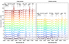 |
Fig. A.1. UV spectrum for deep (left) versus shallow (right) models across evolution (from bottom to top). |
All Tables
Variable input parameters of the PoWR models along the evolutionary tracks of the nonrotating 150 M⊙ models.
Output of effective photospheric temperature of the different models in kilokelvins.
All Figures
|
Fig. 1. Hertzsprung-Russell diagram showing the evolution of the nonrotating models of potential VMS computed with GENEC using the updated mass-loss scheme. Each track is labeled with the corresponding initial mass (in M⊙). The red and blue markers represent the ZAMS and TAMS, respectively. The color of the tracks indicates the surface hydrogen content across the evolution. |
| In the text | |
|
Fig. 2. Hertzsprung-Russell diagram showing the evolution of the 150 M⊙ models computed with GENEC using the new mass-loss scheme. The initial velocity of the rotating model was set at 10% of the critical velocity. The markers (labeled 00−15) represent the evolution snapshots used to compute atmosphere models with PoWR along the nonrotating track. The color of the tracks indicates the evolving surface hydrogen content of the models. |
| In the text | |
|
Fig. 3. Evolution of the interior atmospheric structure of the continuum optical depth (top) and the total Rosseland mean opacity (bottom) of a nonrotating 150 M⊙ star during the MS. The dashed red line shows the location of τ = 20, and the dashed black line marks a local density of 10−7 g cm−3. These represent the connection boundary for the atmosphere models outlined in Sect. 3.2. |
| In the text | |
|
Fig. 4. Optical spectrum for deep (left) vs. shallow (right) models across evolution (from bottom to top). The spectra are vertically offset so that the continuum level corresponds to the grid point number on the y axis for easy reading. The spectral types were estimated based on the classification scheme in Crowther & Walborn (2011). |
| In the text | |
|
Fig. 5. Fitting of the deep model spectrum with a shallow model of varying mass-loss rates at grid point 06. The original prescribed mass-loss rate used for the main models (green and yellow) and the evolutionary track is given in the boxed text for comparison. |
| In the text | |
|
Fig. 6. Density stratification across the MS evolution of the two PoWR model series compared to the GENEC structure models. The grid points correspond to the locations shown on the HRD in Fig. 2. The x axis represents the modified radial coordinate 1 − Rdeep/r, where Rdeep is the lower boundary radius R* of the deep model. This scaling allows us to visualize both the inner part and the wind domain of the atmosphere (see, e.g., figures in González-Torà et al. 2025; Debnath et al. 2024). |
| In the text | |
|
Fig. 7. Temperature stratification across the MS evolution of the two PoWR model series as well as the GENEC structure models. The grid points correspond to the locations shown on the HRD in Fig. 2. For the PoWR models, the electron temperature is shown. |
| In the text | |
|
Fig. 8. Stratification of the neutral hydrogen number fraction for the models at grid points 03 and 04 for the 150 M⊙ track, showing the appearance of a recombination region for the shallow models at grid point 04. The subsequent shallow models in the series look qualitatively similar to the grid point 04 shallow model shown here, whereas no prominent recombination peak appears for any of the deep models. |
| In the text | |
|
Fig. 9. Evolution of the atmospheric profile of the Rosseland and flux-weighted mean opacities of the PoWR models, as well as the tabulated Rosseland mean opacity of the GENEC models. The opacity threshold for which the radiative acceleration surpasses gravity, as calculated by Eq. (5), is also shown. |
| In the text | |
|
Fig. 10. Evolution of the 150 M⊙ star on the HRD using different methods to obtain the effective photospheric temperature T2/3. The solid black line shows the unmodified output of the GENEC track, and the square and circle scatter points show the output of the PoWR deep and shallow model series along the evolutionary track. The five nonsolid lines follow the approximated wind-corrected photospheric temperature calculated from the GENEC structure models via the method outlined in Sect. 5.5 using different assumptions for the connection radius Rcon (see main text for details). |
| In the text | |
|
Fig. A.1. UV spectrum for deep (left) versus shallow (right) models across evolution (from bottom to top). |
| In the text | |
Current usage metrics show cumulative count of Article Views (full-text article views including HTML views, PDF and ePub downloads, according to the available data) and Abstracts Views on Vision4Press platform.
Data correspond to usage on the plateform after 2015. The current usage metrics is available 48-96 hours after online publication and is updated daily on week days.
Initial download of the metrics may take a while.