| Issue |
A&A
Volume 698, June 2025
|
|
|---|---|---|
| Article Number | A262 | |
| Number of page(s) | 27 | |
| Section | Stellar atmospheres | |
| DOI | https://doi.org/10.1051/0004-6361/202554421 | |
| Published online | 20 June 2025 | |
Very massive stars at low metallicity: Evolution, synthetic spectroscopy, and impact on the integrated light of starbursts
1
LUPM, Univ. Montpellier, CNRS,
Montpellier,
France
2
Observatoire de Genève, Université de Genève,
Chemin Pegasi 51,
1290
Versoix,
Switzerland
★ Corresponding author: This email address is being protected from spambots. You need JavaScript enabled to view it.
Received:
7
March
2025
Accepted:
2
May
2025
Abstract
Context. Very massive stars (VMSs), with masses in excess of 100 M⊙, are known in the Galaxy and the Large Magellanic Cloud (LMC). They are mostly characterised by their strong stellar winds compared to normal massive stars. Their mass-loss rates have been calibrated at the metallicity of the LMC. No constraints exist at other metallicities.
Aims. We aim to study the spectroscopic appearance of VMSs and their effect on the integrated light of starbursts at low metallicity.
Methods. In the absence of empirical constraints, we adopted two frameworks for the mass-loss rates of VMSs: in one case, we assumed no metallicity dependence; in the other case, we assumed a linear scaling with metallicity. Under these assumptions, we computed evolutionary models for masses 150, 200, 250, and 300 M⊙ at Z = 0.2, 0.1 and 0.01 Z⊙. We computed the associated synthetic spectra at selected points along the evolutionary tracks. Finally, we built population synthesis models including VMSs based on our new VMS models.
Results. We find that the evolution of VMSs depends critically on the assumptions regarding mass-loss rates. In case of no metallicity dependence, VMSs remain hot for all their lifetimes. Conversely, when mass-loss rates are reduced because of lower metallicity, VMSs follow a classical evolution towards the red part of the Hertzsprung-Russell diagram. VMSs display He II 1640 emission in most phases of their evolution, except when they become too cool. This line is present in the integrated light of population synthesis models down to 0.1 Z⊙ whatever the star formation history, and is also sometimes seen at Z = 0.01 Z⊙. He II 1640 is weaker in models that include a metallicity scaling of the mass-loss rates. The optical spectra of starbursts, especially the Wolf-Rayet bumps, sometimes display VMS signatures when these stars are present. At low metallicities, adding VMSs to population synthesis models produces more ionising photons down to ~45 eV. At higher energies, the ionising flux depends on age, metallicity, assumptions regarding VMS mass-loss rates, and on the very short phases at the end of VMS evolution. He II ionising fluxes large enough to produce some amount of nebular He II 4686 emission can be produced under specific circumstances. Our models are able to reproduce qualitatively and sometimes also quantitatively the UV spectra of star-forming regions. However, we are not able to clearly identify which mass-loss framework is favoured.
Conclusions. Very massive stars can be identified down to 0.1 Z⊙, and potentially to 0.01 Z⊙ depending on the mass-loss rates’ metallicity scaling, through their He II 1640 emission. Their detailed evolution at these low metallicities, especially their mass-loss rates, can be constrained when more UV spectra of star-forming regions at low metallicities are available.
Key words: stars: early-type / stars: evolution / stars: massive / stars: mass-loss / galaxies: starburst
© The Authors 2025
 Open Access article, published by EDP Sciences, under the terms of the Creative Commons Attribution License (https://creativecommons.org/licenses/by/4.0), which permits unrestricted use, distribution, and reproduction in any medium, provided the original work is properly cited.
This article is published in open access under the Subscribe to Open model. This email address is being protected from spambots. You need JavaScript enabled to view it. to support open access publication.
1 Introduction
The mass of the most massive stars is unset. Based on observations of Feitzinger et al. (1980), Cassinelli et al. (1981) determined a mass of 2500 M⊙ for the R136 object at the core of giant H II region 30 Doradus (30 Dor), in the Large Magellanic Cloud (LMC). High spatial observations subsequently revealed that R136 is a cluster of stars rather than a unique object. A ‘canonical’ upper mass limit of 150 M⊙ was for some time promoted by Figer (2005), before a new analysis of the R136 objects established that stars with masses up to 200–300 M⊙ exist in that cluster (Crowther et al. 2010; Bestenlehner et al. 2020; Brands et al. 2022). So far these mass estimates appear robust enough against further decomposition of the R136 objects into more pieces (Kalari et al. 2022; Sabhahit et al. 2025). In particular, binarity is excluded by the most recent Hubble Space Telescope observations (Shenar et al. 2023). The existence of stars with masses in excess of 100 M⊙ is thus robustly established. These stars are referred to as very massive stars (VMSs, Vink 2015).
Because of the shape of the initial mass function, VMSs are rare. Outside of R136, individual VMSs have been observed in the Galactic clusters NGC 3603 (Schnurr et al. 2008; Crowther et al. 2010) and the Arches (Martins et al. 2008). All clusters have masses in excess of about 104 M⊙ (e.g. Stolte et al. 2006). A few other relatively isolated objects reach the mass limit to be classified as VMSs (Hamann et al. 2006; Barniske et al. 2008; Bestenlehner et al. 2011). In spite of being rare objects, Crowther et al. (2016) show that VMSs can dominate the integrated ultraviolet (UV) light of clusters. In particular, the He II 1640 emission of R136 is only produced by the few VMSs it hosts. This property can be used to infer the presence of VMSs in star-forming regions, even if they are not resolved into their individual components (Martins et al. 2023). The presence of VMSs is thus considered likely in the clusters NGC3125-A (Wofford et al. 2014, 2023), II Zw-40-A (Leitherer et al. 2018), NGC5352-5 (Smith et al. 2016), and MrK71-A (Smith et al. 2023). Beyond the local Universe Upadhyaya et al. (2024) explain the morphology of the rest-frame UV spectra of intensely star-forming galaxies by the presence of VMSs. Senchyna et al. (2021) argue that accounting for all stellar emission and nebular lines of starburst galaxies in the local Universe is only feasible with population synthesis models that include VMSs. The most powerful starburst galaxies detected at redshift 2–4 also show spectroscopic features that can be attributed to VMSs (Marques-Chaves et al. 2020, 2021, 2022).
Very massive stars efficiently process chemical elements in their interior and release new material in their close environment (e.g. Higgins et al. 2023). This has raised interest in them to explain the properties of nitrogen emitters, which are starforming regions or galaxies showing a ratio of nitrogen to oxygen abundance higher than what is commonly seen at a given metallicity. These objects have been known for a couple of decades (Villar-Martín et al. 2004; James et al. 2009; Patrício et al. 2016), but their existence in the early Universe, as has been discovered by JWST observations (Bunker et al. 2023; Isobe et al. 2023; Ji et al. 2024; Castellano et al. 2024; Pascale et al. 2023; Schaerer et al. 2024; Senchyna et al. 2024), has placed them on the front line. The surprising nitrogen content has been tentatively explained by normal Wolf-Rayet (WR) stars, supermassive stars, but also by VMSs (Cameron et al. 2023; Charbonnel et al. 2023; Higgins et al. 2023; Vink 2023; Marques-Chaves et al. 2024).
Besides their mass, VMSs are mostly characterised by their high luminosities and high mass-loss rates. The resulting rich spectrum of emission lines makes VMSs appear as hydrogen-rich WN stars, although they are in fact main-sequence stars for most of their lifetime. In hot massive stars, winds are radiatively driven (Castor et al. 1975; Kudritzki et al. 1989; Puls et al. 2000) and the associated mass-loss rates mostly scale with luminosity. For VMSs, the mass-loss rates determined from spectroscopic analysis do not follow the relation established for lower mass O-type stars: they are stronger, sometimes by nearly a factor of 10 (Martins et al. 2008; Bestenlehner et al. 2014). This is explained by the proximity to the Eddington limit (Gräfener & Hamann 2008; Vink et al. 2011). Recent studies have established a relation between the mass-loss rates of VMSs and their Eddington factor (Bestenlehner 2020; Gräfener 2021). These relations are calibrated for the metallicity of the LMC, since they rely on observational data in 30 Dor. In a previous study, we adopted one such calibration to study the spectroscopic evolution of VMSs in the LMC (Martins & Palacios 2022). We show that the inclusion of VMS spectra in population synthesis models produce for the first time the observed He II 1640 emission of young star-forming regions. Schaerer et al. (2025) used these models to quantify the impact of VMSs on the ionising properties of star-forming regions.
The behaviour of VMS mass-loss rates at different metallicities is unknown. The number of VMSs observed in the Galaxy is small, and they are presently not seen at sub-LMC metallicities because of observational limitations (distance, spatial resolution of current observing facilities). Consequently no scaling relation for their mass-loss rates exists outside of the LMC. Theoretical models for the winds of VMSs do not exist at present. Predictions for hydrogen-poor and less massive WR stars indicate a complex relation between mass loss, metallicity, and the Eddington parameter (Sander & Vink 2020). These models are only partly relevant for VMSs, which are usually hydrogen-rich. Large hydrogen fractions are known to affect line-driving (Gräfener & Hamann 2008). Sabhahit et al. (2023) developed a framework to predict VMS mass-loss rates at different metallicities, but empirical confirmation of the predicted trends is pending. In the present study, we explore different assumptions regarding VMS mass-loss rates to investigate their spectroscopic appearance at low metallicity.
The remaining of the paper is organised as follows. Sect. 2 describes our method and assumptions. In Sect. 3 we describe our results in terms of evolutionary models and synthetic spectra. The latter are used in Sect. 4 to build population synthesis models that are tested against observations of low metallicity star-forming regions. We discuss our findings in Sect. 5 and conclude in Sect. 6.
2 Method
The method we used is the same as that presented in Martins & Palacios (2022). We first computed evolutionary models with mass-loss rate recipes adapted for VMSs. We then computed atmospheric models and synthetic spectra along the evolutionary tracks. Both evolutionary and atmospheric models are consistent in the sense that the output of evolutionary models are used as inputs for the computation of atmospheric models. The resulting synthetic spectra were subsequently used to build population synthesis models that include VMS.
We performed our computations for three different metallicities: 0.2, 0.1, and 0.01 Z⊙. This choice is mostly driven to cover the range of metallicity of local and high redshift star-forming galaxies. Fig. 6 of Vanzella et al. (2023) illustrates that Z varies between ~0.5 and 0.02 Z⊙ for a compilation of these objects, with a clear floor at 0.01 Z⊙1. Recent JWST observations (e.g. Nakajima et al. 2023; Chemerynska et al. 2024) indicate that metallicities below 1% of the solar metallicity are so far not observed, except in very rare candidates (Vanzella et al. 2023; Fujimoto et al. 2025). We provided models at Z = 0.4 Z⊙ in Martins & Palacios (2022). In the present study we aim at sampling the metallicity range described above, with 0.2 Z⊙ corresponding roughly to the Small Magellanic Cloud value and to the bulk of the samples shown in Vanzella et al. (2023), 0.1 Z⊙ being a representative value of low metallicity star-forming galaxies and 0.01 Z⊙ setting the lower limit of the metallicity range.
2.1 Mass-loss recipe at low Z
The first step was to select the mass-loss recipe relevant for VMS mass-loss rates at low metallicity. As is described in Sect. 1, no empirical recipe exists, and theoretical predictions are either partial or uncalibrated. We thus adopted a pragmatic approach.
Empirical studies have shown that the winds of normal WR stars vary with Z. Crowther et al. (2002) reported a reduction of mass-loss rates of WC stars in the LMC compared to Galactic counterparts. The analysis of Galactic, LMC, and SMC WR stars by Sander et al. (2012, 2014); Hainich et al. (2014, 2015); Hamann et al. (2019) revealed a global metallicity dependence of the form ![Mathematical equation: $\[\dot{M} \propto Z^{1.2 \pm 0.1}\]$](/articles/aa/full_html/2025/06/aa54421-25/aa54421-25-eq1.png) . But other parameters controlling the wind strength, such as the Eddington factor and/or the mass to light ratio, are hidden in this global scaling. For the specific case of VMSs, Smith et al. (2023) present UV spectroscopy of the massive cluster A in the galaxy MrK 71. Its metallicity is estimated to be 0.16 Z⊙ from nebular lines (Chen et al. 2023). The weakness of C IV 1550 confirms a relatively low metal content. However, He II 1640 appears to be strong with a shape similar to that of VMSs in R136. From this observation Smith et al. (2023) conclude that the winds of VMSs do not depend on Z. Sabhahit et al. (2023) present a theoretical framework for mass loss of VMSs at low metallicity. They describe how the transition between normal and boosted mass-loss rate should change with Z. No empirical confirmation of this scheme has been performed so far. Sander & Vink (2020) performed hydrodynamical simulations of stellar winds of WR stars with no hydrogen and studied the dependence of the mass loss with the Eddington factor (Γe) and the metal content. They find that for a given Γe the metallicity dependence is weak, but that the transition Γe from thin to thick winds varies strongly with Z, implying that low Z WR stars with relatively small Γe have reduced mass-loss rates. However, as demonstrated early on by Gräfener & Hamann (2008) massloss rates of VMSs depend sensitively on the hydrogen mass fraction.
. But other parameters controlling the wind strength, such as the Eddington factor and/or the mass to light ratio, are hidden in this global scaling. For the specific case of VMSs, Smith et al. (2023) present UV spectroscopy of the massive cluster A in the galaxy MrK 71. Its metallicity is estimated to be 0.16 Z⊙ from nebular lines (Chen et al. 2023). The weakness of C IV 1550 confirms a relatively low metal content. However, He II 1640 appears to be strong with a shape similar to that of VMSs in R136. From this observation Smith et al. (2023) conclude that the winds of VMSs do not depend on Z. Sabhahit et al. (2023) present a theoretical framework for mass loss of VMSs at low metallicity. They describe how the transition between normal and boosted mass-loss rate should change with Z. No empirical confirmation of this scheme has been performed so far. Sander & Vink (2020) performed hydrodynamical simulations of stellar winds of WR stars with no hydrogen and studied the dependence of the mass loss with the Eddington factor (Γe) and the metal content. They find that for a given Γe the metallicity dependence is weak, but that the transition Γe from thin to thick winds varies strongly with Z, implying that low Z WR stars with relatively small Γe have reduced mass-loss rates. However, as demonstrated early on by Gräfener & Hamann (2008) massloss rates of VMSs depend sensitively on the hydrogen mass fraction.
In this context we decided to adopt a pragmatic and empirical approach for the present study. Since there is no clear mass-loss recipe for VMSs at metallicities lower than that of the LMC, we simply assumed two representative cases. In the first one, we followed Smith et al. (2023) and assumed no Z-dependence. We thus adopted the recipe of Gräfener (2021) as in our previous study at Z = 1/2.5 Z⊙ (Martins & Palacios 2022). In the second case, we assumed a Z scaling close to that pointed out by Hainich et al. (2015) for classical WR stars, i.e. we scaled the mass-loss rates of Gräfener (2021) according to ![Mathematical equation: $\[\dot{M} \propto\left(\frac{Z}{Z_{L M C}}\right)^{1.0}\]$](/articles/aa/full_html/2025/06/aa54421-25/aa54421-25-eq2.png) , since the recipe of Gräfener (2021) is calibrated for metallicity of the LMC. Regarding the transition between optically thin and thick winds, we sticked to the recipe of Gräfener (2021) and assumed no variation with metallicity. Our models should thus produce two relatively different sets of spectroscopic sequences for VMSs at low Z that can be compared to observed spectra of star-forming regions hosting VMSs.
, since the recipe of Gräfener (2021) is calibrated for metallicity of the LMC. Regarding the transition between optically thin and thick winds, we sticked to the recipe of Gräfener (2021) and assumed no variation with metallicity. Our models should thus produce two relatively different sets of spectroscopic sequences for VMSs at low Z that can be compared to observed spectra of star-forming regions hosting VMSs.
2.2 Stellar evolution models
As in our previous work (Martins & Palacios 2022), we computed stellar evolution models with the STAREVOL code adopting the following physical ingredients: a grey atmosphere as outer boundary to the stellar structure equations, mixing length theory to treat the energy transport in convective regions with αMLT = 1.6304, step core overshooting with αov = 0.1Hp, and Hp the pressure scale height, and solar scaled chemical compositions for Z = 0.002216 (0.2 Z⊙), Z = 0.0013446 (0.1 Z⊙) and Z = 0.00013446 (0.01 Z⊙) with respect to the solar reference chemical composition by Asplund et al. (2009). No α-elements enhancement was considered2. We used the OPAL opacity tables for the corresponding set of solar-scaled abundances, and nuclear rates extracted from the NetGen server and including NACRE II rates for the light elements up to oxygen (Xu et al. 2013).
The mass-loss recipe was from Gräfener (2021) as in Martins & Palacios (2022) with a different treatment of the optically thin and thick winds and a metallicity-dependence of the optically thick winds as follows:
![Mathematical equation: $\[\begin{aligned}\log \left(\dot{M}_{\text {thin }}\right)= & -6.697~( \pm 0.061) \\& +2.194~( \pm 0.021) \times ~\log \left(\frac{L_*}{10^5}\right) \\& -1.313~( \pm 0.046) \times ~\log \left(\frac{M_*}{30}\right)\\& -1.226~( \pm 0.037) \times ~\log \left(\frac{v_{\infty} / v_{\text {esc }}}{2}\right) \\& +0.933~( \pm 0.064) \times ~\log \left(\frac{T_{\text {eff }}}{40000}\right) \\& -10.92~( \pm 0.90) \times ~\log \left(\frac{T_{\text {eff }}}{40000}\right)^2 \\& +0.85~( \pm 0.10) \times ~\log \left(\frac{Z}{Z_{\odot}}\right) \\\end{aligned}\]$](/articles/aa/full_html/2025/06/aa54421-25/aa54421-25-eq3.png) (1)
(1)
![Mathematical equation: $\[\log \left(\dot{M}_{\text {thick }}\right)=\left(5.22 \log \left(\Gamma_{\mathrm{e}}\right)-0.5 \log (D)-2.6\right)\left(\frac{Z}{Z_{\mathrm{LMC}}}\right)^x,\]$](/articles/aa/full_html/2025/06/aa54421-25/aa54421-25-eq4.png) (2)
(2)
where ![Mathematical equation: $\[\dot{M}\]$](/articles/aa/full_html/2025/06/aa54421-25/aa54421-25-eq5.png) is in M⊙/yr, L* and M* are the luminosity and mass of the star in solar units, Teff is the effective temperature in Kelvin, the ratio between terminal and escape velocities v∞/vesc is taken equal to 2.6 as in Eq. (24) of Vink et al. (2001), Z⊙ = 0.019, D = 10 the wind clumping factor, x is taken equal to 0 (mass-loss rate independent of metallicity) or to 1 (Z-scale for the mass-loss rates of VMSs), and Γe is the Eddington factor:
is in M⊙/yr, L* and M* are the luminosity and mass of the star in solar units, Teff is the effective temperature in Kelvin, the ratio between terminal and escape velocities v∞/vesc is taken equal to 2.6 as in Eq. (24) of Vink et al. (2001), Z⊙ = 0.019, D = 10 the wind clumping factor, x is taken equal to 0 (mass-loss rate independent of metallicity) or to 1 (Z-scale for the mass-loss rates of VMSs), and Γe is the Eddington factor:
![Mathematical equation: $\[\Gamma_e=10^{-4.813}(1+X) \frac{L}{L_{\odot}} \frac{M_{\odot}}{M}.\]$](/articles/aa/full_html/2025/06/aa54421-25/aa54421-25-eq6.png)
The switch between the two mass-loss regimes was assumed to occur under the same circumstances as those prescribed by Gräfener (2021) for the LMC, which is to say:
![Mathematical equation: $\[\begin{aligned}& \text { if } \tau_{s}<\frac{2}{3} \text { then optically thin regime } \rightarrow \dot{M} \equiv \dot{M}_{\text {thin }} \\& \text { if } \tau_{s}>1 \text { then optically thick regime } \rightarrow \dot{M} \equiv \dot{M}_{\text {thick}},\end{aligned}>1 \text { then optically thick regime} \rightarrow \dot{M} \equiv \dot{M}_{\text {thick}},\]$](/articles/aa/full_html/2025/06/aa54421-25/aa54421-25-eq7.png)
with τs the sonic-point optical depth that, for a stellar model with a surface mass, M, luminosity, L, radius, R, and hydrogen mass fraction, X, reads:
![Mathematical equation: $\[\tau_{s} \approx \frac{\dot{M} v_{\infty}}{L / c}\left(1+\frac{v_{\mathrm{esc}}^{2}}{v_{\infty}^{2}}\right).\]$](/articles/aa/full_html/2025/06/aa54421-25/aa54421-25-eq8.png)
In the intermediate regime (2/3 ≤ τs ≤ 1), the mass loss is obtained by a linear interpolation between ![Mathematical equation: $\[\dot{M}_{\text {thin}}\]$](/articles/aa/full_html/2025/06/aa54421-25/aa54421-25-eq9.png) and
and ![Mathematical equation: $\[\dot{M}_{\text {thick}}\]$](/articles/aa/full_html/2025/06/aa54421-25/aa54421-25-eq10.png) to ensure a smooth transition.
to ensure a smooth transition.
We focused on models with initial masses of 150, 200, 250, and 300 M⊙ and for each mass, we computed the evolution from the zero-age main sequence (ZAMS) to the end of core He burning for most models3 including mass loss without Z-scaling in the optically thick wind regime. This represents more than 99% of the total lifetime of the modelled stars.
2.3 Atmosphere models
We computed atmosphere models at selected points along evolutionary tracks corresponding to ages of 0, 0.5, 1, 1.5, and 2 Myr. An additional point was added in most tracks, corresponding either to 2.5 Myr or to a representative age between 2.0 and 2.5 Myr for the most massive models not reaching 2.5 Myr. The position of the selected points on the stellar tracks is shown by the symbols in Fig. 1, and the corresponding physical parameters are listed in Tables A.1 to A.4.
We used the code CMFGEN (Hillier & Miller 1998) to compute the atmosphere models. CMFGEN solves the radiative transfer equation under non-local thermodynamical equilibrium conditions. It uses a spherical geometry to include expanding stellar winds. A quasi-hydrostatic solution of the momentum equation is connected to a velocity law of the form ![Mathematical equation: $\[v=v_{\infty} \times\left(1-\frac{R}{r}\right)^{\beta}\]$](/articles/aa/full_html/2025/06/aa54421-25/aa54421-25-eq11.png) with v∞ the maximum velocity at the top of the atmosphere, r the radial coordinate and β a parameter fixed to 1.0 in our calculations. The density structure follows from the velocity structure and the equation of mass conservation. Thousands of lines from various species and their ions are included for a realistic atmospheric structure and emergent spectrum. The final spectrum results from a formal solution of the radiative transfer with the atmospheric structure fixed. Detailed line profiles are used and a micro-turbulent velocity varying from 10 to
with v∞ the maximum velocity at the top of the atmosphere, r the radial coordinate and β a parameter fixed to 1.0 in our calculations. The density structure follows from the velocity structure and the equation of mass conservation. Thousands of lines from various species and their ions are included for a realistic atmospheric structure and emergent spectrum. The final spectrum results from a formal solution of the radiative transfer with the atmospheric structure fixed. Detailed line profiles are used and a micro-turbulent velocity varying from 10 to ![Mathematical equation: $\[0.1 \times v_{\infty} \mathrm{\tilde{k}{m}} \mathrm{~s}^{-1}\]$](/articles/aa/full_html/2025/06/aa54421-25/aa54421-25-eq12.png) is included to account for the observed extra-broadening of lines.
is included to account for the observed extra-broadening of lines.
The surface properties of the evolutionary models at the selected points were used as input to the atmospheric computations, ensuring full consistency. In particular the surface abundances predicted by the evolutionary models were used to predict the corresponding spectral appearance. As was already demonstrated in our previous study (Martins & Palacios 2022), this is important to correctly predict the strength of key VMS lines, especially He II 1640.
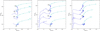 |
Fig. 1 HR diagram for models at Z = 0.2(0.1, 0.01) Z⊙ in the left (middle, right) panel. In each panel the blue (cyan) lines are models without (with) metallicity scaling of the VMS mass-loss rates. Squares and circles correspond to the points where atmosphere models and synthetic spectra are calculated. Crosses correspond to the models discussed in Sect. 5.2. |
3 Results
We present our results first focusing on the evolutionary paths in the Hertzsprung-Russell (HR) diagram. We then describe the spectroscopic appearance of our VMS models in the UV and optical range, as well as the shape of their ionising flux.
3.1 Stellar evolution and VMS mass-loss rates
We show in Fig. 1 the evolutionary tracks of the various models. When decreasing the metallicity, the ZAMS point barely moves, the effective temperature at the beginning of core H burning differs by at most 5% in the mass range considered, meaning that luminosity almost directly scales with mass independently of the temperature, which is expected for such stars (Yusof et al. 2013). The shape of the evolutionary tracks for a given mass-loss recipe is also independent of the initial mass, the tracks simply being shifted to higher luminosities for larger initial masses.
The major difference encountered between all tracks is then due to the metallicity scaling applied to the mass-loss recipe for the optically thick winds regime. The models that have reduced mass-loss rates because of the metallicity scaling evolve classically towards the red part of the HR diagram. To better understand this evolution, and the difference with the other mass-loss scenario we explore, we show in Fig. 2 the opacity profile of our models at different ages. During evolution the total mass is reduced at a relatively slow pace during the main-sequence evolution so that the luminosity increase is important. As the surface temperature slowly decreases during the early main-sequence evolution, it reaches values lower than that associated with HeII ionisation (log (THeII bump) ≈ 4.6) – see left panel, Fig. 2. A HeII opacity bump is built below the surface that triggers convection and causes a further radius inflation (Cantiello et al. 2009; Grassitelli et al. 2021) that drives the evolution to the red in the HR diagram for these models.
Such a bump never appears in the models that maintain a higher mass loss (see Fig. 2, right panel). More specifically, these models remain close to the zero-age main sequence (ZAMS) for most of the main-sequence evolution, which lasts approximately 2.5 Myr. They subsequently evolve to the blue in the core He fusion phase (which lasts for ≈10% of the main-sequence lifetime) where they remain for the very last phases (which represent less than 0.5% of the main-sequence lifetime). The main-sequence duration is longer in these models despite their convective core being less massive. This is essentially due to the lack of a heavy envelope on top of that core, which reaches lower temperatures than in models of the other family discussed above, thus causing a slower evolution on the main sequence. Indeed for these models, the star is stripped by mass loss with M⋆ decreasing by ≈55% to 62% (for the 150 M⊙ and 300 M⊙ at the three metallicities considered) of its initial value over the duration of the main sequence (see Tables A.1 to A.4). As the envelope mass decreases, the portion of the total mass occupied by the H core is very large (80% to 90%) and does not evolve much during the main sequence. Consequently these models have a quasi-homogeneous evolution at this phase, and are thus expected to evolve to the blue (Maeder 1987; Langer 1992; Farrell et al. 2020). As H is processed into He in the core, the overall mean molecular weight of the stellar plasma ![Mathematical equation: $\[\bar{\mu}\]$](/articles/aa/full_html/2025/06/aa54421-25/aa54421-25-eq13.png) increases during the main sequence (from 0.65 at the ZAMS to 1.33 at 2 Myr for the 200 M⊙ model at 0.1 Z⊙). A rough estimate gives
increases during the main sequence (from 0.65 at the ZAMS to 1.33 at 2 Myr for the 200 M⊙ model at 0.1 Z⊙). A rough estimate gives ![Mathematical equation: $\[L_{\star} \propto M_{\star}^{3} \bar{\mu}_{\star}^{4}\]$](/articles/aa/full_html/2025/06/aa54421-25/aa54421-25-eq14.png) : the increase in
: the increase in ![Mathematical equation: $\[\bar{\mu}\]$](/articles/aa/full_html/2025/06/aa54421-25/aa54421-25-eq15.png) balances the strong decrease in M⋆, which leads to a very modest luminosity variation during the main sequence.
balances the strong decrease in M⋆, which leads to a very modest luminosity variation during the main sequence.
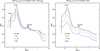 |
Fig. 2 Mean Rosseland opacity profiles as a function of temperature at four different ages on the main sequence for the 200M⊙ model at 0.1 Z⊙ with (left) and without (right) Z-scaling of the VMS mass-loss rates. The opacity bumps of CNO nuclei, Fe and He II are indicated. |
3.2 Spectroscopic evolution
We now proceed with the description of the spectroscopic evolution of low metallicity VMS. We illustrate the general behaviour of our models with the 200 M⊙ model at Z = 0.1 Z⊙4. The optical and UV spectra at different evolutionary points along the tracks plotted in Fig. 1 are shown in Fig. 3. The left panels illustrate the evolution when no metallicity scaling of the VMS mass-loss rates is applied. In this case the star remains hot at all times, and barely evolves from its ZAMS position as discussed in the previous section. Consequently the spectral morphology is little affected by changes in ionisation and the spectra exhibit almost the same lines at different evolutionary phases. However, variations in surface abundances and mass-loss rate affect the strength of these lines. In the optical, this is seen in He II 4686 that is the main feature. He II 1640 follows the same trend in the UV: it is already present on the ZAMS and becomes stronger when the star evolves, moving from a P-Cygni profile to a pure emission profile in the last model. We also note the strengthening of N IV 1486 and N IV 1720 as evolution proceeds. The physical reasons for this temporal evolution have been described in Martins & Palacios (2022). As evolution proceeds, VMSs are more and more chemically processed at their surface, showing the products of CNO burning, in particular nitrogen and helium enrichment (see Tables A.3). At the same time mass-loss rates are increased because of the larger Eddington factor, driven by the larger luminosity-to-mass ratio. These two effects produce the strong helium and nitrogen lines observed in the spectra of VMSs.
The evolutionary sequence is quite different when VMS mass-loss rates are scaled with metallicity. The spectra are thus affected (right panels of Fig. 3). Because of the reduced wind density many lines are now in absorption. The Balmer lines turn into emission at the end of the evolutionary sequence because of the reduction in temperature and increase in wind density. He II 4686 is always in emission but is weaker than in the case where VMS mass-loss rates are not scaled with Z. We note the presence of a weak C IV 5802-12 doublet in emission for most models. In the UV the decrease in temperature along the evolution is clearly seen in the shift of the dominating iron ion, from Fe VI on the ZAMS (upper spectrum) to Fe IV in the most evolved model (lower spectrum). O V 1371 is present on the ZAMS and disappears, whereas Si IV 1393-1403 develops into a strong double P-Cygni profile in the most evolved phases.
The behaviour of spectra at Z = 0.2 Z⊙ is qualitatively similar to that of Z = 0.1 Z models (see Appendix B). There are some quantitative differences though. Obviously with a larger metal content the iron line forests in the UV are stronger at Z = 0.2 Z⊙ (see Figs 3 and B.1). In the optical we have seen that C IV 580212 shows a double-peaked profile in Z = 0.1 Z⊙ models. This was also seen at higher metallicity (Martins & Palacios 2022). This is also true of Z = 0.2 Z⊙ models close to the ZAMS, but more evolved models with no Z scaling of mass-loss rates show a broad profile. This is attributed to a still relatively large carbon content and at the same time a hot temperature and a high mass-loss rate. These conditions are gathered only in these models. At higher Z evolved models are cooler, and at lower Z the carbon content is reduced. The morphology of C IV 5802-12 has been used as a criterion to identify VMSs in star-forming galaxies (Martins et al. 2023). We will get back to this in Sect. 4.4.
At Z = 0.01 Z⊙ the changes are more pronounced. The lower metal content translates into an almost complete disappearance of the iron forests in the UV. In the high mass-loss rate scenario He II 1640 remains clearly present and dominates this wavelength range for most of the evolution. Longward of 1200 Å, only Lyα and N V 1240 remain visible past the first 0.5 Myr of evolution. This is due to a combination of hot temperature and chemical processing at the surface that for instance reduce the strength of C IV 1550. For mass-loss rates scaled with metallicity the UV spectrum resembles, for the first time in our modelling of VMSs, that of O-type stars. He II 1640 is still present but is weak and does not dominate the UV spectrum. Similarly He II 4686 is mostly in absorption and does not stand out as a peculiar line. If VMS mass-loss rates scale linearly with metallicity VMSs cannot be distinguished from normal main-sequence massive stars at very low metallicity.
Fig. 4 illustrates the spectral differences in the 200 M⊙ models after 1 Myr of evolution, at the three metallicities considered in this work. The models correspond to the case of no Z scaling of mass-loss rates. The optical range is dominated by He II lines and their morphologies are rather similar regardless of the metallicity. In the UV lines are mostly similar between Z = 0.2 and 0.1 Z⊙, while most metallic lines disappear at Z = 0.01 Z⊙. From Tables A.1, A.3 and A.5 we see that the helium content is the same in all three models (Y~0.28) but the nitrogen and carbon content decreases by more than a factor of 10 as Z decreases, leading to the disappearance of C IV 1550 and N IV 1720 for instance. But metallicity also has an indirect effect: Teff is higher at lower Z, thus affecting the ionisation balance. This translates into a weakening of N IV lines, while N V 1240 remains strong in spite of the reduced nitrogen content.
Metallicity has an impact of the spectroscopy of VMS. The largest effects are those related to the scaling or not of VMS mass-loss rates with Z, since this affects both stellar evolution and spectroscopic appearance. However, the main conclusion is that down to Z = 0.1 Z⊙ whatever the exact Z scaling, He II 1640 is always seen in emission and dominates the UV spectrum. This feature is the most emblematic of VMS. It is still the strongest emission at Z = 0.01 Z⊙ if VMS mass-loss rates do not scale with Z. Otherwise, He II 1640 emission vanishes. We thus expect very young stellar population hosting VMSs to show He II 1640 in emission over a wide range of metallicity. We further investigate this in Sect. 4.
In Sect. 3.1, we saw that the shape of evolutionary tracks is, to first order, qualitatively the same for different initial masses, at a given metallicity. One may thus wonder whether one can use the synthetic spectra computed along one track and simply scale them according to luminosity to obtain those of another mass. Fig. 5 shows that this is not possible. The four synthetic spectra correspond to four different initial masses, but the same age (1 Myr). They have similar Teff (~55 to 56 kK) so that the ionisation is rather comparable in the four models. In spite of this lines are not the same in all four spectra. In particular He II 1640 and He II 4686 show clear sequences of increased strength with mass. This is explained by the higher helium mass fraction and larger mass-loss rates when mass increases. Inspection of Table A.1 indicates that Y ranges from 0.251 to 0.369 for initial masses between 150 and 300 M⊙, at 1 Myr. At the same time the mass-loss rates increases from 10−4.73 to 10−4.14 M⊙ yr−1, because the Eddington factor increases. In Fig. 5 we also notice that N IV 1486 is stronger in higher mass models, and C IV 5802-12 is weaker. This is also a consequence of chemical mixing that exposes the products of CNO burning at the surface, i.e. nitrogen enrichment and carbon depletion (see Table A.1). The conclusion from this comparison is that it is not possible to scale synthetic spectra according to their luminosity to obtain the spectra of more luminous stars, since not only mass-loss rates but also surface composition changes. Proper modelling of spectra along all tracks with different initial masses is necessary for quantitative predictions of the spectral appearance of VMS.
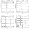 |
Fig. 3 Synthetic optical (top) and UV (bottom) spectra of the 200 M⊙ models at Z = 0.1 Z⊙. The left (right) panels correspond to models without (with) metallicity scaling of the mass-loss rates. In all panels, the spectra from top to bottom correspond to models with 0.01, 0.5, 1, 1.5, 2, and 2.5(2.2) Myr as marked by squares on the evolutionary track in Fig. 1 and with parameters given in Tables A.3 and A.4. Spectra are shifted vertically for clarity. |
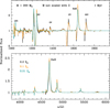 |
Fig. 4 Spectra of the 200 M⊙ models at 1 Myr for Z = 0.2 Z⊙ (black), 0.1 Z⊙ (orange) and 0.01 Z⊙ (cyan). Models have no metallicity scaling of the mass-loss rates. The top (bottom) panel shows the UV (optical) range. |
4 Population synthesis
We now proceed to the inclusion of VMS models into population synthesis models. We describe the method and then discuss the impact of VMSs on the integrated light of starbursts. We highlight the effects of metallicity. We confront our models to observations of three clusters suspected to host VMSs.
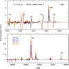 |
Fig. 5 Spectra of the Z = 0.2 Z⊙ models after 1 Myr, for the four initial masses considered in this work. Models have no metallicity scaling of the mass-loss rates. The top (bottom) panel shows the UV (optical) range. |
4.1 Model set-up
We proceeded as in Martins & Palacios (2022) to build population synthesis models including VMS. For normal stars with masses below 100 M⊙ we retrieved the BPASS models of Eldridge et al. (2017). We selected models with an upper IMF slope of −2.35 and no binaries. We chose the BPASS models with metallicities Z = 0.002, 0.001 and 10−4 since they are the closest ones for our Z = 0.2, 0.1 and 0.01 Z⊙ VMS models, respectively. We then extended the mass function up to 225 M⊙ using our 150 and 200 M⊙ models as representative of stars in the mass bins 100–175 and 175–225 M⊙. For test models we extended the upper mass cut-off up to 300 M⊙, with the VMS 250 and 300 M⊙ models representing stars in the mass range 225–275 and 275–300 M⊙, respectively. We proceeded as in Upadhyaya et al. (2024) to correct for the bug in the formal description of the mass function presented by Eldridge et al. (2017). For all ages the contribution of VMSs was added to the BPASS models, and we re-normalised the final fluxes so they correspond to a total mass of 106 M⊙. BPASS does not provide burst models for ages 0 and 0.5 Myr, so for these ages we added the 1 Myr BPASS models to our 0 and 0.5 Myr populations of VMS. Most of our models reach 2.5 Myr, but some stop just short of it (e.g. the 200 M⊙ model at Z = 0.2 Z⊙ and scaled mass-loss rates, for which the age is 2.4 Myr – see Table A.2). In that case we make the assumption that these models with ages ≲2.5 Myr are still representative at 2.5 Myr and we use them to produce the population spectrum at that age. For constant star formation (CSF) models we simply added the contributions of bursts weighted by the duration of the age range they represent. In practice we divided time into the following ranges (expressed in Myr): 0–0.25, 0.25–0.75, 0.75–1.25, 1.25–1.75, 1.75–2.25, 2.25–2.75, 2.75–3.0, 3.0–4.0, 4.0–5.0, 5.0–6.0, 6.0–8.0, 8.0–10.0, 10.0–12.5, 12.5–16.0, 16.0–20.0, 20.0–25.0, 25.0–32.0, 32.0–40.0 and 40.0–50.0. For each of these ranges we used, respectively, the bursts with age: 0, 0.5, 1.0, 1.5, 2.0, 2.5, 3.0, 4.0, 5.0, 6.0, 8.0, 10.0, 12.5, 16.0, 20.0, 25.0, 32.0, 40.0, and 50.0 Myr.
 |
Fig. 6 UV spectra of burst models for ages between 1 and 2.5 Myr. Coloured lines are models including VMSs, black lines models without VMSs (i.e. BPASS models). The dark (light) colours correspond to mass-loss rates not scaled (scaled) with metallicity. The left (middle, right) panel is for Z = 0.2 (0.1, 0.01) Z⊙. |
4.2 Spectral morphology
We show how our models compare to BPASS models without VMSs in Fig. 6. As already found for Z = 1/2.5 Z⊙ (Martins & Palacios 2022) He II 1640 emission is produced only by models that include VMSs, making this feature a unique tracer of their presence in young stellar populations. He II 1640 is stronger in models where the VMS mass-loss rates are not scaled with metallicity, which is expected. In that case it is present at all times. If a metallicity scaling is applied, He II 1640 disappears at 2.5 Myr because of the different evolution: VMSs become cool so that He II recombines into He I – see bottom panels of Fig. 6, cyan lines. At low metallicity N IV 1720 is strongly affected by the presence of VMSs, as was the case at Z = 1/2.5 Z⊙. The presence of a broad emission around N IV 1486 is also caused by VMSs. We thus confirm previous findings that VMSs uniquely affect the UV spectra of young starbursts. We also note that other features are strengthened by the presence of VMSs: N V 1240, O V 1371, and C IV 1550. In models with metallicity scaling of mass-loss rates Si IV 1393-1403 appears as a strong doublet at 2.5 Myr, and is almost entirely due to VMSs. As anticipated from the discussion of spectra of individual stars, these conclusions vanish in the case where Z = 0.01 Z⊙ and VMS mass-loss rates scale with Z (left panel of Fig. 6, light colours). Here, VMSs have little effect on the integrated spectrum. Except for this extreme case, VMSs thus manifest themselves in the integrated spectrum of young starbursts over a wide range of metallicities, regardless of their exact mass-loss rates. This indicates that UV spectroscopy should be able to probe the presence of VMSs over a wide range of metallicity, and in most star-forming regions known to date.
This conclusion holds as long as only VMSs are present or dominate completely the light emitted by massive stars. If in addition to them classical WR stars co-exist in sufficient number, things may get more complicated. Although the current generation of population synthesis models that include WR stars is not able to produce any He II 1640 in emission as observed, empirical results on 30 Dor show that normal WR stars may still contribute some flux (Crowther & Castro 2024). This calls for a revision of the inclusion of WR stars in population synthesis models. In any case, the relative role of VMSs and normal WR stars can be distinguished based on the morphology of the optical features we describe in Sect. 4.4 (see also Martins et al. 2023).
Altogether these results indicate that the characteristic features of VMSs at Z = 1/2.5 Z⊙ remain tracers of their presence in starbursts at lower metallicity. We now examine in more detail the effects of metallicity on these and other spectroscopic quantities.
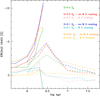 |
Fig. 7 EW (He II 1640) as a function of age for burst models (solid lines) and CSF models (dashed lines). Models with Z = 0.2(0.1, 0.01) Z⊙ are shown in red and pink (blue and cyan, orange and yellow). Light colours (pink, cyan, and yellow) are models with a metallicity scaling of mass-loss rate, while blue, red, and orange are models with no Z scaling. Green lines are models from Martins & Palacios (2022) at Z = 0.4 Z⊙. |
4.3 He II 1640
In Sect. 3.2, we saw that He II 1640 was produced in emission in most of our low metallicity models of individual VMS. We now investigate how the strength of this line varies with Z in young stellar populations. For that we calculate its equivalent width (EW) over the wavelength range 1625–1655 Å. This range encompasses the widest extension encountered in the He II 1640 profile of all our models. We plot EW(He II 1640) versus age in Fig. 7. In addition to the models calculated for the present paper we also add those of Martins & Palacios (2022) at Z = 0.4 Z⊙. For these latter models, there is only one recipe for VMS mass-loss rate: that of Gräfener (2021).
Fig. 7 shows how EW(He II 1640) varies with age for burst and CSF models. Since He II 1640 strengthens as VMSs evolve off the ZAMS, we see an increase in its EW with age in all models up to 2.5 Myr. After that VMSs and their He II 1640 emission disappear. Consequently EW(He II 1640) decreases in CSF models after 2.5 Myr. The models with VMS mass-loss rates that are not scaled with metallicity show the highest EWs, up to 10 Å in burst models and 4 Å in CSF models. In bursts models with the strongest mass-loss rates EW(He II 1640) is on average larger at lower metallicity, except at 2.5 Myr. The reasons for this behaviour are rooted in the shape of the line profiles that are illustrated in Fig. 8. When metallicity decreases the absorption lines that are superimposed on He II 1640 are weaker so the emission near 1640 Å is higher. In addition at lower metallicity He II 1640 shifts from a P-Cygni profile to an emission profile. Consequently the absorption part disappears thus pushing the EW to higher values. The reason for the change of profile of He II 1640 is that stars are less compact at higher metallicity, leading to a smaller escape velocity at their surface. Since the maximum velocity of the wind is directly proportional to the escape velocity, it is reduced at higher metallicity. This affects the wind density and thus the shape of the stellar lines formed in the wind. This is clearly seen in Fig. 8 where the dark red profile is more centrally peaked, with a stronger absorption dip in the P-Cygni profile. On the contrary the orange profile (Z = 0.01 Z⊙) is purely in emission.
In burst models with VMS mass-loss rates scaling with metallicity He II 1640 emission is reduced. EW(He II 1640) still reaches a maximum of 1.5 Å at Z = 0.2 Z⊙. Below that metallicity there is almost no emission. In CSF models the same trends are observed qualitatively. Low metallicity models produce slightly higher EW than the highest Z models, and models with reduced mass-loss rates have EW (He II 1640) close to zero after ~3 Myr. This does not mean that there is no He II 1640 emission, as illustrated by the pink and cyan lines in the right panel of Fig. 8: a weak emission is detected. But over the wavelength range considered for the EW measurement, absorption lines compensate for this emission.
Conti & Morris (1990) proposed a method to determine dust extinction based on the relative strength of He II 1640 and He II 4686 in WR stars. Their study is based on the assumption that both lines arise from recombination processes in optically thin nebulae so that their strength mostly relies on atomic physics. Thus in standard physical conditions this ratio is equal to 7–8 (Seaton 1978; Hummer & Storey 1987). Leitherer et al. (2019) measured line flux ratios in Galactic and LMC WR stars and show that a correlation exists with a line ratio of 7.76. Thus, comparing observed ratios to dust-free ratios allows for the determination of dust attenuation, as is done in Maschmann et al. (2024). In Fig. 9, we show the luminosity of He II 1640 compared to He II 4686. Only models that clearly show both lines in emission are considered for this figure. The wavelength region over which the luminosity is calculated is tailored for each model, in order to take into account the full line width. A correlation between L (He II 1640) and L (He II 4686) is seen. It follows relatively well the relation empirically determined by Leitherer et al. (2019). The points that deviate the most correspond to CSF models with mass-loss rates that scale with metallicity, and at low metallicity. In those cases lines are weak and measurements are more uncertain, especially for He II 4686.
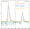 |
Fig. 8 Profile of He II 1640 for burst models at 2.5 Myr (left panel) and 3 Myr CSF models (right panel). Different colours correspond to different metallicities and assumptions regarding VMS mass-loss scaling with Z, and are explained in the right panel. |
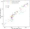 |
Fig. 9 Luminosity of He II 1640 as a function of luminosity of He II 4686 for burst (triangles) and CSF (open squares) models at various metallicities. Metallicities and assumptions regarding mass-loss rates are indicated in the upper left part of the figure. The dotted line shows the relation reported by Leitherer et al. (2019). |
4.4 Optical bumps
Martins et al. (2023) show that distinguishing young star forming regions dominated by VMSs from those where classical WR stars are present can be done using the morphology of the emission features near 4630–4690 Å and 5800–5820 Å, the so-called WR bumps. When only VMSs are present the blue feature shows a He II 4686 emission with no or little N III 4634-42 emission. The red bump is also different depending on the population: VMSs produce a double narrow emission sometimes on top of a broader but weak emission, while WR stars form a broad and strong emission feature without narrow doublet.
In Fig. 10, we show the morphology of the blue and red WR bumps in our models that include VMSs. The blue bump never shows N III 4634-42 emission, whatever the star-formation history and the assumption regarding VMS mass loss. He II 4686 goes from a weak feature to a strong emission. It is stronger for higher mass-loss rates, as expected. The maximum emission is seen in burst models at 2.5 Myr of CSF models at 3 Myr, when the contribution of VMSs with respect to other stars is maximum. For models with a metallicity scaling of VMS mass-loss rates the He II 4686 emission is usually weak and disappears at the lowest metallicity. For CSF models with age larger than ~10 Myr the blue bump is also weak or absent.
In most models the red bump is characterised by the narrow C IV doublet emission. A broader and weak component is sometimes observed underneath the doublet. For CSF models the red bump is very weak or absent.
For the metallicity range considered, VMSs may not always manifest themselves through the optical bumps. If a strong He II 4686 emission is seen, N III 4634-42 is absent. The red bump may or may not be seen. When present it is most of the time dominated by the narrow C IV doublet.
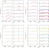 |
Fig. 10 Morphology of the optical blue and red bumps in burst models. Different colours correspond to different metallicities (see left panels). The top (bottom) panels correspond to models without (with) Z scaling of the VMS mass-loss rates. The left panels show burst models in which age goes from 0 (top) to 2.5 Myr (bottom) with 0.5 Myr increments. The right panels show CSF models with age 3, 5, 8, 10, 20, and 50 Myr from top to bottom. |
4.5 lonising flux
In this section, we first compare the shape of the ionising spectrum of stellar populations hosting VMSs. For this we plot the cumulative number of ionising photons above energy E and normalised to the value at 13.6 eV (which corresponds to the Lyman break). Fig. 11 shows this quantity for burst models at 1 and 2 Myr, and for the same metallicities as in the previous Section. The Z = 0.4 Z⊙ case at 1 Myr is discussed by Schaerer et al. (2024) who highlight that the shape of the ionising spectrum is basically unaffected by the presence of VMSs below 35 eV. At higher energies VMSs lead to a reduction of the ionising flux, mostly because of their dense winds.
The second, third, and fourth columns of Fig. 11 present the Z = 0.2, 0.1 and 0.01 Z⊙ cases, respectively. Compared to the Z = 0.4 Z⊙ case there is a global trend of more ionising photons in models with VMSs compared to models without them, as metallicity decreases. At 1 Myr the choice of the mass-loss rate has little impact on the number of ionising photons below ~47 eV. This is different above that energy, and especially true for He II ionising photons. Models without metallicity scaling of the VMS mass-loss rates produce fewer He II photons than models with weaker winds. At Z = 0.2 Z⊙ the former have less ionising photons than the BPASS models, while the latter have more ionising photons. Below Z = 0.1 Z⊙ all models with VMSs produce more He II ionising photons than the BPASS models. As described in Schaerer et al. (2025) the presence of weaker winds leads to a reduced opacity in the He II continuum that translates into more flux.
At 2 Myr (bottom panels of Fig. 11) models with VMSs and Z = 0.4 Z⊙ have a significantly softer ionising spectrum compared to models without VMSs. The reason is that at that age VMSs are evolved and cooler than the bulk of less massive stars. The VMSs thus contribute less flux at high energies, leading to a softer spectrum of the population. At 2 Myr the choice of the mass-loss rate recipe for low metallicity VMSs has an impact on the shape of the ionising continuum. Indeed, depending on the mass-loss history, a VMS will evolve to the red part of the HRD, thus becoming cooler, or will stay in the hot part of the HRD, and will produce ionising photons (see Fig. 1). The bottom panels of Fig. 11 show this effect: below ~45 eV the dark lines, corresponding to the un-scaled VMS mass-loss rates, are above the light ones, corresponding to Z-scaled mass-loss rates. Regarding the He II ionising flux, only the lowest metallicity models produce more photons than models without VMSs.
For completeness we show in Fig. 12 Q(>E) for 10 Myr CSF models. As is seen in burst models, a reduction in metallicity translates into a larger number of ionising photons with E<45 eV in models with VMSs, compared to non-VMS models. Above 54 eV only the Z = 0.01 Z⊙ models produce more ionising photons (right panel). Above that metallicity models with and without VMSs produce a rather similar ionising continuum.
In conclusion, as the shape of the ionising flux is concerned, there is a global trend of more ionising photons below ~45 eV when VMSs are included with strong mass-loss rates. For higher energies and for models with lower mass-loss rates the behaviour is more complex, depends on age, star formation history and energy. As discussed in Sect. 5.2 the treatment of the most advanced phases of evolution also shapes the SED at these energies in a way that remains difficult to quantify at present.
Fig. 13 shows the effects of metallicity on the number of ionising photons for our models that include VMSs. In addition to H I, He I, and He II we also show the Ne II photon flux since it corresponds to an energy of 40.9 eV close to the energy separating the spectral regions where the effects of the assumptions on mass-loss rate on the shape of the SED are best seen. When metallicity decreases there is a global trend of more ionising photons. The difference is the smallest for H I and increases at higher energies as discussed above. We also see that Q(He II) has a relatively complex behaviour as already stressed (see also Sect. 5.2). Fig. 13 also confirms the trend reported by Schaerer et al. (2025) that VMSs increase the number of H I and He I ionising photons by a factor of ~2. Again, the behaviour of the number of He II ionising photons is more complex, with no clear trend with metallicity.
Finally, Fig. 14 shows the ionising photon efficiency, ξion, defined as the ratio of the number of hydrogen ionising photons to the luminosity at 1500 Å (in units of erg/s/Hz). A reference value for log(ξion) is 25.2 erg−1 Hz, as was defined by Robertson et al. (2013) based on population synthesis models that do not include VMSs (Bruzual & Charlot 2003). The models shown in Fig. 14 include the nebular continuum emission on top of the stellar emission. To add this contribution, we followed the method described in Schaerer (2002), with the various coefficients taken from Osterbrock & Ferland (2006). Nebular emission includes free-free and free-bound emission by H, neutral He, and He+. Hydrogen two photon emission was also taken into account. An electron temperature of 10 000 K and an electron density of 100 cm−3 were adopted.
Schaerer et al. (2025) show that ξion is boosted by the presence of VMSs and more generally by a top-heavy initial mass function. The models of Fig. 14 confirm this trend: for a given metallicity, the models that include VMSs have systematically larger ξion values compared to the BPASS models (that do not include VMSs). The novelty seen in Fig. 14 compared to the work of Schaerer et al. (2025) is the metallicity dependence of ξion. Taking the CSF models at 10 Myr as an example, log(ξion) increases from 25.55 at Z = 0.4 Z⊙ to 25.62 at Z = 0.1 Z⊙, and up to 25.69 at Z = 0.01 Z⊙. For comparison the BPASS models produce log(ξion) = 25.39 to 25.56 for the same metallicity range. The increase in ξion also depends on the mass-loss assumption for VMS. The models that produce the largest ionising photon efficiency are those with the higher mass-loss rates. This is mostly because these models remain hot, leading to a large ionising photon flux. Measurements of log(ξion) in star-forming galaxies at high redshift often reach values of 25.5 to 26.0, as summarised in Fig. 8 of Seeyave et al. (2023). Such values are difficult to explain with standard models (i.e. without VMSs) unless bursts of age ≲5 Myr are invoked. Our models release part of the tension with empirical measurements, offering the possibility to reach large ξion at low metallicity.
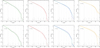 |
Fig. 11 Number of photons above energy E for Z = 0.4 Z⊙, 0.2 Z⊙, 0.1 Z⊙ and 0.01 Z⊙ (from left to right). Lighter and heavier colours in each panel correspond to models with (without) Z-scaling of the VMS mass-loss rates. The black and grey lines correspond to the BPASS model in each panel. The top (bottom) panels are for an age of 1(2) Myr. Vertical dotted lines mark the ionisation energy of selected ions. |
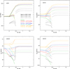 |
Fig. 13 Number of ionising photons per second as a function of age for population synthesis models. The upper left (upper right, lower left, lower right) panel is for H I (He I, He II, Ne II). Solid (dashed) lines are burst (CSF) models. Grey lines are for BPASS models that do not include VMSs, i.e. the models we use for stars with masses below 100 M⊙. |
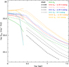 |
Fig. 14 Ionising photon efficiency as a function of age. Different colours are used for different metallicities and assumption regarding VMS mass-loss rate, as is explained in the upper right corner of the figure. Solid (dashed) lines are for burst (CSF) models that include nebular continuum emission. |
4.6 Comparison to local starbursts
In this section, we compare our population synthesis models including VMSs to spectroscopic observations of low metallicity starburst clusters or galaxies in the local Universe. The UV data used for the comparisons, all from the Hubble Space Telescope (HST), are described in Table 1 and have been retrieved from the MAST database. We selected all sources that show He II 1640 in emission and for which the metallicity estimates are within the range of our models. We found three objects that fulfil these criteria: cluster A in II Zw 40, cluster A in MrK71, and the starburst region SB-126.
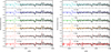 |
Fig. 15 Comparison between burst population synthesis models including VMSs up to 225 M⊙ and the observed UV spectrum of the super star cluster in II Zw 40. All models are for Z = 0.2 Z⊙. Ages range from 0 to 2.5 Myr from top to bottom. The left (right) panels correspond to models without (with) metallicity scaling of the VMS mass-loss rates. |
HST/COS data for starbursts.
4.6.1 II Zw 40-A
Cluster A in the galaxy II Zw 40 was studied by Leitherer et al. (2018) who show that it has one of the strongest He II 1640 emission among local starbursts. UV spectroscopy reveals the presence of all the strong lines seen in VMSs and Leitherer et al. (2018) suspect that VMSs are indeed present in the cluster. In Fig. 15 we compare the predictions of our population synthesis models at different ages with the UV spectrum of II Zw 40-A. The right and left panels correspond to models that have VMS mass-loss rates that scale (do not scale) with metallicity. The metallicity of II Zw 40 is 12+log(O/H) = 8.09, close to that of the SMC (Guseva et al. 2000) so we use our models for Z = 0.2 Z⊙ in Fig. 15. A direct by-eye inspection indicates that the global morphology of the observed spectra is qualitatively reproduced: He II 1640 is predicted in emission, C IV 1550 is well developed, N IV 1720 is present. O V 1371 is also predicted but systematically stronger than the observation. Among the two families of models, the 1.5 Myr model with no metallicity scaling of the mass-loss rates (orange in the left panel) is particularly remarkable since it reproduces fairly well most observed features. The quality of this fit is not matched by models in which the mass-loss rates are scaled with metallicity. In those models He II 1640 is too weak compared to the observed spectrum, or is reasonably reproduced but at the cost of a too strong C IV 1550.
To better appreciate the comparisons, we show in Fig. 16 a zoom on the two strongest features, C IV 1550 and He II 1640. The only model of the Z-scaling series that reaches the level of He II 1640 emission of II Zw 40 is that at 2 Myr. But as stressed above the corresponding C IV 1550 P-Cygni profile is too strong. For the no Z-scaling mass-loss models, we see again that the 1.5 Myr model provides an almost perfect match to C IV 1550 and He II 1640. Leitherer et al. (2018) determined an age of 2.8±0.1 Myr for the cluster, from the comparison of the strongest UV features with Starburst99 models restricted to masses below 100 M⊙. They could not reproduce He II 1640 (see their Fig. 3). Since VMSs contribute not only to He II 1640 but also to other UV lines, stronger lines are produced at earlier times which explains the slightly younger age we favour.
So far our population synthesis models include VMSs up to 225 M⊙. Increasing the upper mass limit to 300 M⊙ slightly boosts the UV emission, especially that of He II 1640. But this is not sufficient to affect qualitatively the conclusions raised above: the best-fit model remains one of the series without Z-scaling of the VMS mass-loss rates, and the models with scaled mass-loss rates suffer from the same limitations as above. With the He II 1640 emission increase when the upper mass limit is extended, the model of the no Z-scaling series at an age of 1 Myr becomes equivalent to that at 1.5 Myr.
4.6.2 MrK71-A
The UV spectrum of cluster A in the galaxy MrK71 displays strong lines produced in the winds of massive stars. The He II 1640 emission is particularly strong, relative to other lines such as C IV 1550. As was described in Sect. 1, Smith et al. (2023) attribute this to the presence of VMSs and argue that their mass-loss rates do not depend on Z. MrK71 has 12+log(O/H) = 7.89 (Chen et al. 2023) slightly below the SMC value. We overplot our Z = 0.2 Z⊙ burst models including VMSs on top of the UV spectrum of MrK71-A in Fig. 17. Unlike for II Zw 40, no model reproduces quantitatively all features. In particular the relative strength of C IV 1550 and He II 1640 is not matched. C IV 1550 is weak, which is attributed to the low metallicity of the galaxy (Smith et al. 2023). All of our models at Z = 0.2 Z⊙ and that have no Z scaling of the VMS mass-loss rates overpredict the C IV 1550 strength. For the same metallicity, the models with Z scaling of the mass-loss rates and age 0 and 0.5 Myr reproduce reasonably the C IV 1550 emission, but underpredict He II 1640. At later ages, the strength of He II 1640 increases and matches the observed profile, but then C IV 1550 is way too strong. A possible solution to this issue could be that the age of the cluster is lower than 1 Myr. As is explained in Sect. 4.1 BPASS does not provide burst models below 1 Myr so we used the 1 Myr BPASS models for the population of normal massive stars at 0 and 0.5 Myr. Since normal O stars contribute to C IV 1550 that strengthens with time, we suspect that the use of the 1 Myr BPASS models at 0 and 0.5 Myr leads to an over-prediction of the C IV 1550 strength. However, the strength of O V 1371 would be even larger in that case, which is opposite to what would be needed to solve the mismatch with C IV 1550.
We checked whether a lower metallicity would be helpful. The Z = 0.1 Z⊙ models are shown in the lower panels of Fig. 17. When no Z scaling of mass-loss rates is considered, He II 1640 is reproduced at 0.5 Myr, when C IV 1550 is slightly over-predicted. The same argument as above for C IV 1550 would help to reduce its strength a bit, bringing the model and observed spectra into better agreement. For the case of Z scaling of mass-loss rates, He II 1640 reaches the observed emission strength between 1.5 and 2 Myr, but C IV 1550 is too strong by that age.
Increasing the upper mass limit of our models does not help, since all lines are affected. When He II 1640 is increased so is C IV 1550 so that the discrepancy we describe above remains. Thus, there is no model with VMSs that quantitatively match the observed UV spectrum of MrK71-A.
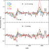 |
Fig. 16 Comparison between burst population synthesis models including VMSs up to 225 M⊙ to the observed UV spectrum of cluster A in II Zw 40 (black line). All models are for Z = 0.2 Z⊙ that is close to the metallicity of the cluster. Ages range from 0 to 2.5 Myr and are colour-coded as indicated in the top panel. The top (bottom) panel corresponds to models without (with) metallicity scaling of the VMS mass-loss rates. The vertical black lines indicate the Galactic nebular C IV absorption. |
4.6.3 SB 126
The starburst galaxy SB-126 was studied by Senchyna et al. (2021). For this source and others they could not match both the stellar wind features and the nebular emission lines at the same time. To solve this issue they invoke the presence of VMSs. SB-126 has a metallicity 12+log(O/H) = 8.02±0.04 according to Senchyna et al. (2021). We show how its UV spectrum compares to our Z = 0.2 Z⊙ models in Fig. 18. Since the UV spectrum of SB 126 likely results from a combination of several sources, as stressed by Senchyna et al. (2021) and visible from their Fig. 2, we use CSF models rather than burst models. The CSF models with ages between 5 and 50 Myr are considered.
The models with no Z scaling of the mass-loss rates of VMSs tend to over-predict He II 1640, although the mismatch is relatively small at ages larger than 20 Myr. Conversely, the strength of this line is slightly underestimated in models with a metallicity scaling of mass loss. The models of this family with ages of 20 to 50 Myr also account reasonably well for C IV 1550. They also fit nicely both N V 1240 and the Si IV doublet near 1400 Å.
For SB-126, reasonable fits of the UV spectrum can be obtained. This is an improvement compared to the analysis of Senchyna et al. (2021) who needed to consider metallicities higher than measured to reproduce the observed lines of C IV 1550 and He II 1640. In our case there is no such tension regarding metallicity. In spite of this relative success a clear conclusion regarding which family of models (mass-loss Z-scaling or not) is most appropriate to fit the data is not reached. A metallicity scaling of the VMS mass-loss rates that would be shallower than the one adopted here may improve the global fits for this galaxy. However, the fact that the spectrum likely results from several sources complicates the analysis. It may be that some sources contain VMSs, some not, so the resulting spectrum is a combination of several types of spectra.
5 Discussion
In this section, we discuss some of the shortcomings of our modelling regarding stellar evolution, mass-loss rates, and population synthesis.
5.1 VMS evolution
Models of VMSs have been computed by several authors. Yusof et al. (2013) proposed models for stars up to 500 M⊙ at Z = 0.014, 0.004 and 0.002 which correspond to solar, LMC and SMC metallicity. Mass-loss rates are taken from Vink et al. (2001) as for O-type stars, and thus do not include the specific VMS recipes. The resulting evolutionary tracks are characterised by a vertical evolution with a luminosity decrease, over a wide range of masses and metallicities. This is different from the models of Köhler et al. (2015) that have a classical redward evolution. These models are also based on the Vink et al. (2001) mass-loss recipe and thus do not include the boosted winds of VMSs.
Martinet et al. (2023) improve on the Geneva models of Yusof et al. (2013) by, among other things, using the mass-loss recipe of Gräfener & Hamann (2008) for VMSs. A global metallicity dependence of the form (Z/Z⊙)0.7 is assumed. Their models are designed for Z = 0, 10−5, 0.006 and 0.014. The tracks show a complex behaviour. At the metallicity of the LMC (Z = 0.006) that is comparable to our computations (Martins & Palacios 2022), the models of Martinet et al. start with a classical redward evolution down to Teff~30 000 K before evolving mostly to the blue. Their models show a global trend of evolution that extends more to the red part of the HRD as metallicity decreases. The study of Martinet et al. (2023) indicates that as mass increases mass loss becomes the dominant ingredient of VMS modelling. Rotation affects the tracks of their 180 M⊙ models but has almost no impact on the 300 M⊙ track.
Sabhahit et al. (2022) explore two regimes of mass loss for VMS: one based on dependence on the Eddington factor, the other on the luminosity-to-mass ratio. Their computations are for Z = 0.02 and Z = 0.008. For both metallicities the evolution is towards the red for the first mass-loss scheme, and vertically for the second one. Sabhahit et al. favour the latter evolution because observations of VMSs in the Arches cluster and 30 Dor are better accounted for by these models. In a subsequent study they explore the metallicity dependence of the switch from optically thin to optically thick winds (Sabhahit et al. 2023). Their models cover Z = 0.008, 0.004, 0.002, and 0.0002. Their evolution shifts from a vertical one at Z = 0.008 to a horizontal one (to the red of the HR diagram) at Z = 0.002, because of the reduced mass loss.
All these computations show that mass loss is really a key ingredient of the evolution of VMS. Quite different tracks are obtained even if boosted mass-loss rates are included. The exact shape of the dependence of mass-loss rates on physical parameters matters. Unfortunately observational constraints remain too sparse to favour one recipe (see also next Sect. 2.1). The number of individual VMS is small and a preferred position in the HR diagram, as advocated by Sabhahit et al. (2022), is unclear. Adding more stars from other clusters at different ages and metallicities would be most helpful to provide robust constraints.
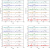 |
Fig. 17 Comparison between burst population synthesis models including VMSs up to 225 M⊙ and the observed UV spectrum of MrK71-A (black line). Top (bottom) models are for Z = 0.2 (0.1) Z⊙. In each panel ages range from 0 to 2.5 Myr from top to bottom. The left (right) panels correspond to models without (with) metallicity scaling of the VMS mass-loss rates. |
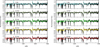 |
Fig. 18 Comparison between Z = 0.2 Z⊙ CSF population synthesis models including VMSs up to 225 M⊙ and the observed UV spectrum of SB 126 (black line). Left (right) panels show models without (with) metallicity scaling of the VMS mass-loss rates. |
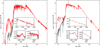 |
Fig. 19 Comparison between the spectrum of the initial CSF population synthesis models at 10 Myr (black line) and the spectrum of a test model in which the contribution of evolved phases of evolution is included (red line). The left (right) panel is for Z = 0.1 (0.01) Z⊙. |
5.2 Advanced phases of evolution
Our population synthesis models do not include the very last phases of evolution. The reasons have been stated in Martins & Palacios (2022). The correct modelling of these advanced phases requires a better ‘coupling’ of evolutionary and atmosphere models than what we do in the present study. Indeed in these phases there is a mismatch in the temperature and density structure of evolutionary and atmosphere models. In addition the advanced phases represent no more than ~10% of the VMS lifetime.
In spite of these limitations, one can still estimate the contribution of the final phases of VMS evolution on the integrated spectra of young starbursts. For this we built test models as follows. We computed new models for the 150 and 200 M⊙ models at Z = 0.1 and 0.01 Z⊙. These models are shown by the cross symbols in the middle and right panels of Fig. 1. Their parameters are listed in Table A.7. The two models on the 150 M⊙ tracks correspond to ages of 2.55 Myr and 2.75 Myr, while the models on the 200 M⊙ tracks have an age of 2.75 Myr. We assume that the 2.55 (2.75) Myr models are representative of the 2.500–2.625 (2.625–2.750) Myr age range in population synthesis models. We recall that stars evolve quickly during their final phases. For instance the Z = 0.1 Z⊙ 150 M⊙ model moves from a position where Teff = 70 kK to Teff = 150 kK in 0.3 Myr so the above assumptions are made to provide a qualitative rather than quantitative assessment of the effect of these shorts evolutionary phases on integrated spectra.
The effect of these advanced phases on the integrated spectrum of starbursts is shown in Fig. 19. The flux is basically unchanged throughout most of the wavelength range. In particular the UV lines, especially He II 1640, are unaffected. The same conclusion holds for the optical bumps. The most notable difference is the increased flux in the He II continuum. The evolved phases correspond to very high effective temperatures not reached in previous phases. Consequently the flux emitted at these wavelengths is boosted. This conclusion should be considered as qualitative rather than quantitative. Indeed, as was stressed above, our test is only a rough estimate of the contribution of evolved phases. A finer sampling of these short phases would be required, together with a better coupling between evolutionary and atmosphere models. Nevertheless our test shows that the UV and optical spectra of CSF models are unaffected by the short advanced phases of VMS evolution. On the other hand, the He II ionising flux is sensitive to these phases.
We estimate the magnitude of this effect in Fig. 20. We show how the ratio of He II to H I ionising photons fluxes changes with time in models that include and do not include these short advanced phases. When VMSs evolve into these phases the ratio reaches values as large as 0.1 for a short amount of time (~0.2 Myr). In CSF models the addition of the advanced phases increases the number of He II ionising photons after 2.5 Myr. Q(He II)/Q(H I) is multiplied by a factor of 10 at Z = 0.1 Z⊙. At lower metallicity the increase is not as large because VMSs are already hot during most of their evolution and produce some amount of He II ionising flux (see Sect. 4.5).
The ratio Q(He II)/Q(H I) reaches 2(5) × 10−3 for CSF models at Z = 0.1 (0.01) Z⊙. Under reasonable approximations (see e.g. Stasińska et al. 2015) it can be converted into the ratio of the intensities of He II 4686 to Hβ: I(He II 4686)/I(H β) = 1.74 × Q(He II)/Q(H I). Consequently CSF models that include the short advanced phases of VMS evolution are able to produce I(He II 4686)/I(Hβ) of the order of 1%. This is sufficient to account for a significant fraction of the observed values in star-forming regions and galaxies where high ionisation lines are observed (e.g. Fig. 1 of Schaerer et al. 2019). However, the predicted intensity ratios are too small to explain the highest observed values, up to 0.06, detected in some sources such as II Zw 18 (Izotov et al. 1997; Kehrig et al. 2015) or SBSS0335052E (Kehrig et al. 2018; Wofford et al. 2021). Burst models caught at 2.5–2.7 Myr would produce these kinds of intensity ratios, but their duration is short enough (~0.2 Myr) to exclude them as a viable explanation for the presence of high ionisation lines.
For the models with scaling of the VMS mass-loss rates with metallicity, the evolution is redwards so the high Teff needed to produce He II ionising flux are not reached. In addition the evolution is faster and stars live shorter than in the case of no metallicity scaling of mass-loss rates. Consequently no effect of these advanced phases is expected in the UV part of the spectrum. These phases thus have a limited impact on the integrated spectral properties of young starbursts that include VMSs.
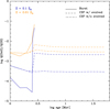 |
Fig. 20 Ratio of He II to H I ionising photons fluxes as a function of age. The dashed (dash-dotted) lines correspond to CSF models in which the advanced phases of evolution are included (not included). In burst models these advanced phases are shown at 2.625 and 2.750 Myr. Blue (orange) lines are for Z = 0.1 (0.001) Z⊙. |
5.3 VMS mass-loss rates at low Z
In this study, we have explored the evolution and spectroscopic appearance of VMSs and associated populations under two assumptions regarding the VMS mass-loss rates. The comparison of population synthesis models with UV spectroscopy of star-forming regions at low metallicity did not allow us to favour one assumption over the other. In both cases He II 1640, the most emblematic feature of VMS, is produced over a wide range of ages and metallicities. Its relative intensity compared to other UV features such as C IV 1550 slightly changes depending on the mass-loss rates. But the confrontation with observations does not help us to distinguish which scenario is correct. In fact the truth may be in between, with a metallicity scaling of mass-loss rates that is shallower than the assumed linear Z dependence.
Sander (2024) present preliminary theoretical modelling of the winds of WN stars. Building on the work of Sander & Vink (2020) for hydrogen-free WN stars, they explore the behaviour of mass-loss rates when hydrogen is present. A rather weak dependence is observed. Combined with the effects of metallicity, the scaling of mass-loss rates appear to be weaker than a linear Z-scaling (see their Fig. 2). However, this exploratory work is for a mass range lower than that of VMSs (by a factor of 10). Further investigation in the VMS regime is thus needed. Sabhahit et al. (2023) propose a framework for the transition between optically thin and thick winds, i.e. between normal O-type stars winds and VMS winds. It relies on the concept of transition mass loss developed by Vink & Gräfener (2012) to parameterise the change between the two winds regimes. Their result indicates that at lower metallicity the boosted mass-loss rates of VMSs appear at higher luminosity. Sabhahit et al. (2023) use their formalism to produce evolutionary models of VMS. Different paths are obtained depending on metallicity and mass. There is a global trend of more redward evolution at lower metallicity, because of reduced winds. This is consistent with our results: we have shown that the models with the lowest VMS mass-loss rates evolve redwards.
Whatever VMS mass-loss recipe we adopt, it appears clear that observational tests are necessary to better understand VMS winds and evolution. The observation of individual VMS in different environments is challenging. There are currently very few star-forming regions that are 1) massive enough, 2) young enough, and 3) close enough for VMSs to be spectroscopically identified and analysed. As is described in Sect. 1, this leaves no more than a dozen VMSs. Future telescopes and instrumentation may be able to break star-forming regions currently unresolved into their stellar components. However, taking R136 as a reference template, spatial resolution of the order 10 mas will be required for the best candidate clusters (such as NGC3125-A, MrK71-A). While this may be possible from an imaging perspective for ELTs and later on HWO, this is a challenge for spatially resolved spectroscopy.
One may thus look for alternative observational tests to better constrain the mass-loss history and the evolution of VMS. The N-emitters presented in Sect. 1 may be one way. When looking at Tables A.1 to A.6, we see that the surface chemistry of models without Z-scaling of the VMS mass-loss rates is different from that of the models with a Z dependence. Because of the stronger winds, the former models expel more material and expose deeper layers of stars to the surface. More material is thus released in the interstellar environment. These different yields may be probed through the imprint they leave in the surrounding gas. VMSs have been listed as one of the potential sources to explain the large nitrogen fraction in the N-emitters (Charbonnel et al. 2023; Vink 2023; Senchyna et al. 2024). A proper computation of the yields from VMSs can in principle be used to see if one of the two mass-loss scenarios we considered is favoured to explain these peculiar star-forming regions. This will be the subject of a future study.
6 Conclusion
We have presented a study of the evolution and spectroscopic appearance of VMSs at metallicities of Z = 0.2, 0.1, and 0.01 Z⊙. We have assumed two mass-loss recipes for their winds. The first one assumes no metallicity dependence of VMS winds, and relies on the calibration of Gräfener (2021) established for VMSs in the LMC. The second recipe assumes a linear scaling with Z, with the Gräfener (2021) as an anchor point. We have computed evolutionary models for stars with initial masses of 150, 200, 250, and 300 M⊙, with the code STAREVOL. We have calculated atmosphere models and synthetic spectra along evolutionary tracks (code CMFGEN), from the ZAMS to ages of about 2.5 Myr (depending on initial mass) with time steps of 0.5 Myr. The resulting spectra have been incorporated in population synthesis models to study the impact of VMSs on the integrated light of star-forming regions.
The main results are summarised as follows:
The evolution of VMSs critically depends on the assumed mass-loss rate recipe. When mass-loss rates do not vary with metallicity, VMSs at low metallicity spend most of their lifetime close to the ZAMS before evolving to the blue part of the HR diagram. On the contrary stars with reduced mass-loss rates at lower metallicity follow a more classical evolution to the red part of the HR diagram;
The UV spectrum of VMSs shows a number of emission and P-Cygni lines typical of massive stars, with a significant He II 1640 emission that is a specific characteristic of VMS. This line is seen down to Z = 0.1 Z⊙ whatever the assumed VMS mass-loss rate recipe. Even at Z = 0.01 Z⊙ the models with the strongest mass-loss rates still show this line in emission;
In the optical range, the WR bumps are seen over a wide range of parameters. The blue bump is dominated by He II 4686 with no of very weak N III 4634-42 emission. When present the red bump shows a narrow C IV 5802-12 doublet emission, sometimes on top of a broader but weak component;
The UV spectrum of population synthesis models have EW(He II 1640) reaching up to 10 Å for bursts, and 4 Å for constant star-formation history. Low-metallicity models predict, on average, larger EW(He II 1640) than models at Z = 0.4 Z⊙. We confirm that only models including VMSs produce He II 1640 in emission;
The ionising spectrum of VMSs is harder at lower metallicities, between 13.6 and ~45 eV. It is also harder than that of models without VMSs. Models with VMS mass-loss rates that do not scale with metallicity, and thus remain hot in the HR diagram, show the hardest spectra. At energies higher than 45 eV, the behaviour is more complex, and is also affected by the very final phases of evolution that are only partially included in the present models. He II ionising photons are produced at a level that can partially account for observed He II nebular lines, although the high intensities sometimes observed are only produced for starbursts at very specific ages. Finally population synthesis models that include nebular emission have higher ionising photon efficiency at lower metallicity;
The UV spectra of three star-forming regions at low metallicity (II Zw 40-A, MrK71-A and SB126) can be matched qualitatively and sometimes quantitatively by burst or CSF models including VMSs. This confirms the importance of including a consistent treatment of VMS evolution and synthetic spectra in population synthesis models of young starbursts. However, no clear trend emerges regarding the preferred mass-loss recipe at low metallicity (i.e. Z-scaling of mass-loss rates or not).
Future spectroscopic identification of individual VMS appears to be difficult, even with the foreseen capabilities. Alternative ways of finding VMSs in spatially unresolved populations may be a better way of constraining VMS properties, in particular their winds. Studies of the chemistry of young star-forming regions, in particular the N-emitters, may also be relevant. Some of these possibilities will be investigated in subsequent publications.
Data availability
The synthetic spectra of individual VMS models are distributed on the POLLUX database at https://pollux.oreme.org/. Evolutionary models and population synthesis models can be shared on reasonable request.
Acknowledgements
We thank an anonymous referee for useful comments. We thank John Hillier for developing and distributing CMFGEN. This research is based on observations made with the NASA/ESA Hubble Space Telescope obtained from the Space Telescope Science Institute, which is operated by the Association of Universities for Research in Astronomy, Inc., under NASA contract NAS 5–26555. These observations are associated with programs 14102, 15185, and 16261.
Appendix A Model parameters
Tables A.1 to A.6 gather the parameters for our sets of models at the three metallicities explored, and for each metallicity with the two assumptions regarding VMS mass-loss rate.
Parameters of the atmosphere models with mass-loss rates not scaled with metallicity and at Z = 0.2 Z⊙.
Parameters of the atmosphere models with mass-loss rates scaled linearly with Z/ZLMC and at Z = 0.2 Z⊙.
Parameters of the atmosphere models with mass-loss rates not scaled with metallicity and at Z = 0.1 Z⊙.
Parameters of the atmosphere models with mass-loss rates scaled linearly with Z and at Z = 0.1 Z⊙.
Parameters of the atmosphere models with mass-loss rates not scaled with metallicity and at Z = 0.01 Z⊙.
Parameters of the atmosphere models with mass-loss rates scaled linearly with Z and at Z = 0.01 Z⊙.
Appendix B Synthetic spectra for additional 200 M⊙ models
In this section, we show the UV and optical spectra of all the individual models of VMS with an initial mass of 200 M⊙. They are complementary to those displayed in Fig. 3. The spectra for all masses are available at the POLLUX database https://pollux.oreme.org/).
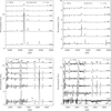 |
Fig. B.1 Synthetic UV (bottom) and optical (top) spectra of the 200 M⊙ models at Z = 0.2 Z⊙. The left (right) panels correspond to models without (with) metallicity scaling of mass-loss rates. |
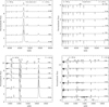 |
Fig. B.2 Synthetic UV (bottom) and optical (top) spectra of the 200 M⊙ models at Z = 0.01 Z⊙. The left (right) panels correspond to models without (with) metallicity scaling of mass-loss rates. |
References
- Asplund, M., Grevesse, N., Sauval, A. J., & Scott, P. 2009, ARA&A, 47, 481 [NASA ADS] [CrossRef] [Google Scholar]
- Barniske, A., Oskinova, L. M., & Hamann, W. R. 2008, A&A, 486, 971 [NASA ADS] [CrossRef] [EDP Sciences] [Google Scholar]
- Bestenlehner, J. M. 2020, MNRAS, 493, 3938 [Google Scholar]
- Bestenlehner, J. M., Vink, J. S., Gräfener, G., et al. 2011, A&A, 530, L14 [NASA ADS] [CrossRef] [EDP Sciences] [Google Scholar]
- Bestenlehner, J. M., Gräfener, G., Vink, J. S., et al. 2014, A&A, 570, A38 [NASA ADS] [CrossRef] [EDP Sciences] [Google Scholar]
- Bestenlehner, J. M., Crowther, P. A., Caballero-Nieves, S. M., et al. 2020, MNRAS, 499, 1918 [Google Scholar]
- Brands, S. A., de Koter, A., Bestenlehner, J. M., et al. 2022, A&A, 663, A36 [Google Scholar]
- Bruzual, G., & Charlot, S. 2003, MNRAS, 344, 1000 [NASA ADS] [CrossRef] [Google Scholar]
- Bunker, A. J., Saxena, A., Cameron, A. J., et al. 2023, A&A, 677, A88 [NASA ADS] [CrossRef] [EDP Sciences] [Google Scholar]
- Cameron, A. J., Katz, H., Rey, M. P., & Saxena, A. 2023, MNRAS, 523, 3516 [NASA ADS] [CrossRef] [Google Scholar]
- Cantiello, M., Langer, N., Brott, I., et al. 2009, A&A, 499, 279 [NASA ADS] [CrossRef] [EDP Sciences] [Google Scholar]
- Cassinelli, J. P., Mathis, J. S., & Savage, B. D. 1981, Science, 212, 1497 [NASA ADS] [CrossRef] [Google Scholar]
- Castellano, M., Napolitano, L., Fontana, A., et al. 2024, ApJ, 972, 143 [Google Scholar]
- Castor, J. I., Abbott, D. C., & Klein, R. I. 1975, ApJ, 195, 157 [Google Scholar]
- Charbonnel, C., Schaerer, D., Prantzos, N., et al. 2023, A&A, 673, L7 [NASA ADS] [CrossRef] [EDP Sciences] [Google Scholar]
- Chemerynska, I., Atek, H., Dayal, P., et al. 2024, ApJ, 976, L15 [NASA ADS] [CrossRef] [Google Scholar]
- Chen, Y., Jones, T., Sanders, R., et al. 2023, Nat. Astron., 7, 771 [Google Scholar]
- Conti, P. S., & Morris, P. W. 1990, AJ, 99, 898 [Google Scholar]
- Crowther, P. A., & Castro, N. 2024, MNRAS, 527, 9023 [Google Scholar]
- Crowther, P. A., Dessart, L., Hillier, D. J., Abbott, J. B., & Fullerton, A. W. 2002, A&A, 392, 653 [NASA ADS] [CrossRef] [EDP Sciences] [Google Scholar]
- Crowther, P. A., Schnurr, O., Hirschi, R., et al. 2010, MNRAS, 408, 731 [Google Scholar]
- Crowther, P. A., Caballero-Nieves, S. M., Bostroem, K. A., et al. 2016, MNRAS, 458, 624 [Google Scholar]
- Eldridge, J. J., Stanway, E. R., Xiao, L., et al. 2017, PASA, 34, e058 [Google Scholar]
- Farrell, E. J., Groh, J. H., Meynet, G., et al. 2020, MNRAS, 495, 4659 [NASA ADS] [CrossRef] [Google Scholar]
- Feitzinger, J. V., Schlosser, W., Schmidt-Kaler, T., & Winkler, C. 1980, A&A, 84, 50 [NASA ADS] [Google Scholar]
- Figer, D. F. 2005, Nature, 434, 192 [Google Scholar]
- Fujimoto, S., Naidu, R. P., Chisholm, J., et al. 2025, ApJ submitted [arXiv:2501.11678] [Google Scholar]
- Gräfener, G. 2021, A&A, 647, A13 [NASA ADS] [CrossRef] [EDP Sciences] [Google Scholar]
- Gräfener, G., & Hamann, W. R. 2008, A&A, 482, 945 [Google Scholar]
- Grassitelli, L., Langer, N., Mackey, J., et al. 2021, A&A, 647, A99 [NASA ADS] [CrossRef] [EDP Sciences] [Google Scholar]
- Guseva, N. G., Izotov, Y. I., & Thuan, T. X. 2000, ApJ, 531, 776 [NASA ADS] [CrossRef] [Google Scholar]
- Hainich, R., Rühling, U., Todt, H., et al. 2014, A&A, 565, A27 [NASA ADS] [CrossRef] [EDP Sciences] [Google Scholar]
- Hainich, R., Pasemann, D., Todt, H., et al. 2015, A&A, 581, A21 [NASA ADS] [CrossRef] [EDP Sciences] [Google Scholar]
- Hamann, W. R., Gräfener, G., & Liermann, A. 2006, A&A, 457, 1015 [NASA ADS] [CrossRef] [EDP Sciences] [Google Scholar]
- Hamann, W. R., Gräfener, G., Liermann, A., et al. 2019, A&A, 625, A57 [NASA ADS] [CrossRef] [EDP Sciences] [Google Scholar]
- Higgins, E. R., Vink, J. S., Hirschi, R., Laird, A. M., & Sabhahit, G. N. 2023, MNRAS, 526, 534 [NASA ADS] [CrossRef] [Google Scholar]
- Hillier, D. J., & Miller, D. L. 1998, ApJ, 496, 407 [NASA ADS] [CrossRef] [Google Scholar]
- Hummer, D. G., & Storey, P. J. 1987, MNRAS, 224, 801 [NASA ADS] [CrossRef] [Google Scholar]
- Isobe, Y., Ouchi, M., Tominaga, N., et al. 2023, ApJ, 959, 100 [NASA ADS] [CrossRef] [Google Scholar]
- Izotov, Y. I., Foltz, C. B., Green, R. F., Guseva, N. G., & Thuan, T. X. 1997, ApJ, 487, L37 [Google Scholar]
- James, B. L., Tsamis, Y. G., Barlow, M. J., et al. 2009, MNRAS, 398, 2 [Google Scholar]
- Ji, X., Übler, H., Maiolino, R., et al. 2024, MNRAS, 535, 881 [NASA ADS] [CrossRef] [Google Scholar]
- Kalari, V. M., Horch, E. P., Salinas, R., et al. 2022, ApJ, 935, 162 [NASA ADS] [CrossRef] [Google Scholar]
- Kehrig, C., Vílchez, J. M., Pérez-Montero, E., et al. 2015, ApJ, 801, L28 [NASA ADS] [CrossRef] [Google Scholar]
- Kehrig, C., Vílchez, J. M., Guerrero, M. A., et al. 2018, MNRAS, 480, 1081 [NASA ADS] [Google Scholar]
- Köhler, K., Langer, N., de Koter, A., et al. 2015, A&A, 573, A71 [NASA ADS] [CrossRef] [EDP Sciences] [Google Scholar]
- Kudritzki, R. P., Pauldrach, A., Puls, J., & Abbott, D. C. 1989, A&A, 219, 205 [NASA ADS] [Google Scholar]
- Langer, N. 1992, A&A, 265, L17 [NASA ADS] [Google Scholar]
- Leitherer, C., Byler, N., Lee, J. C., & Levesque, E. M. 2018, ApJ, 865, 55 [NASA ADS] [CrossRef] [Google Scholar]
- Leitherer, C., Lee, J. C., & Faisst, A. 2019, AJ, 158, 192 [NASA ADS] [CrossRef] [Google Scholar]
- Maeder, A. 1987, A&A, 178, 159 [NASA ADS] [Google Scholar]
- Marques-Chaves, R., Álvarez-Márquez, J., Colina, L., et al. 2020, MNRAS, 499, L105 [Google Scholar]
- Marques-Chaves, R., Schaerer, D., Álvarez-Márquez, J., et al. 2021, MNRAS, 507, 524 [NASA ADS] [CrossRef] [Google Scholar]
- Marques-Chaves, R., Schaerer, D., Álvarez-Márquez, J., et al. 2022, MNRAS, 517, 2972 [CrossRef] [Google Scholar]
- Marques-Chaves, R., Schaerer, D., Kuruvanthodi, A., et al. 2024, A&A, 681, A30 [NASA ADS] [CrossRef] [EDP Sciences] [Google Scholar]
- Martinet, S., Meynet, G., Ekström, S., Georgy, C., & Hirschi, R. 2023, A&A, 679, A137 [NASA ADS] [CrossRef] [EDP Sciences] [Google Scholar]
- Martins, F., Hillier, D. J., Paumard, T., et al. 2008, A&A, 478, 219 [NASA ADS] [CrossRef] [EDP Sciences] [Google Scholar]
- Martins, F., & Palacios, A. 2022, A&A, 659, A163 [NASA ADS] [CrossRef] [EDP Sciences] [Google Scholar]
- Martins, F., Schaerer, D., Marques-Chaves, R., & Upadhyaya, A. 2023, A&A, 678, A159 [NASA ADS] [CrossRef] [EDP Sciences] [Google Scholar]
- Maschmann, D., Leitherer, C., Faisst, A. L., Lee, J. C., & Minsley, R. 2024, ApJ, 961, 159 [Google Scholar]
- Nakajima, K., Ouchi, M., Isobe, Y., et al. 2023, ApJS, 269, 33 [NASA ADS] [CrossRef] [Google Scholar]
- Osterbrock, D. E., & Ferland, G. J. 2006, Astrophysics of gaseous nebulae and active galactic nuclei (Sausalito, CA: University Science Books) [Google Scholar]
- Pascale, M., Dai, L., McKee, C. F., & Tsang, B. T. H. 2023, ApJ, 957, 77 [NASA ADS] [CrossRef] [Google Scholar]
- Patrício, V., Richard, J., Verhamme, A., et al. 2016, MNRAS, 456, 4191 [Google Scholar]
- Puls, J., Springmann, U., & Lennon, M. 2000, A&AS, 141, 23 [NASA ADS] [CrossRef] [EDP Sciences] [Google Scholar]
- Robertson, B. E., Furlanetto, S. R., Schneider, E., et al. 2013, ApJ, 768, 71 [Google Scholar]
- Sabhahit, G. N., Vink, J. S., Higgins, E. R., & Sander, A. A. C. 2022, MNRAS, 514, 3736 [NASA ADS] [CrossRef] [Google Scholar]
- Sabhahit, G. N., Vink, J. S., Sander, A. A. C., & Higgins, E. R. 2023, MNRAS, 524, 1529 [NASA ADS] [CrossRef] [Google Scholar]
- Sabhahit, G. N., Vink, J. S., Sander, A. A. C., et al. 2025, A&A, 696, A200 [NASA ADS] [CrossRef] [EDP Sciences] [Google Scholar]
- Sander, A. A. C. 2024, in IAU Symposium, 361, Massive Stars Near and Far, eds. J. Mackey, J. S. Vink, & N. St-Louis, 473 [Google Scholar]
- Sander, A. A. C., & Vink, J. S. 2020, MNRAS, 499, 873 [Google Scholar]
- Sander, A., Hamann, W. R., & Todt, H. 2012, A&A, 540, A144 [NASA ADS] [CrossRef] [EDP Sciences] [Google Scholar]
- Sander, A., Todt, H., Hainich, R., & Hamann, W. R. 2014, A&A, 563, A89 [NASA ADS] [CrossRef] [EDP Sciences] [Google Scholar]
- Schaerer, D. 2002, A&A, 382, 28 [NASA ADS] [CrossRef] [EDP Sciences] [Google Scholar]
- Schaerer, D., Fragos, T., & Izotov, Y. I. 2019, A&A, 622, L10 [NASA ADS] [CrossRef] [EDP Sciences] [Google Scholar]
- Schaerer, D., Marques-Chaves, R., Xiao, M., & Korber, D. 2024, A&A, 687, L11 [NASA ADS] [CrossRef] [EDP Sciences] [Google Scholar]
- Schaerer, D., Guibert, J., Marques-Chaves, R., & Martins, F. 2025, A&A, 693, A271 [NASA ADS] [CrossRef] [EDP Sciences] [Google Scholar]
- Schnurr, O., Casoli, J., Chené, A. N., Moffat, A. F. J., & St-Louis, N. 2008, MNRAS, 389, L38 [NASA ADS] [CrossRef] [Google Scholar]
- Seaton, M. J. 1978, MNRAS, 185, 5 [Google Scholar]
- Seeyave, L. T. C., Wilkins, S. M., Kuusisto, J. K., et al. 2023, MNRAS, 525, 2422 [NASA ADS] [CrossRef] [Google Scholar]
- Senchyna, P., Stark, D. P., Charlot, S., et al. 2021, MNRAS, 503, 6112 [NASA ADS] [CrossRef] [Google Scholar]
- Senchyna, P., Plat, A., Stark, D. P., et al. 2024, ApJ, 966, 92 [NASA ADS] [CrossRef] [Google Scholar]
- Shenar, T., Sana, H., Crowther, P. A., et al. 2023, A&A, 679, A36 [NASA ADS] [CrossRef] [EDP Sciences] [Google Scholar]
- Smith, L. J., Crowther, P. A., Calzetti, D., & Sidoli, F. 2016, ApJ, 823, 38 [NASA ADS] [CrossRef] [Google Scholar]
- Smith, L. J., Oey, M. S., Hernandez, S., et al. 2023, ApJ, 958, 194 [NASA ADS] [CrossRef] [Google Scholar]
- Stasińska, G., Izotov, Y., Morisset, C., & Guseva, N. 2015, A&A, 576, A83 [NASA ADS] [CrossRef] [EDP Sciences] [Google Scholar]
- Stolte, A., Brandner, W., Brandl, B., & Zinnecker, H. 2006, AJ, 132, 253 [NASA ADS] [CrossRef] [Google Scholar]
- Upadhyaya, A., Marques-Chaves, R., Schaerer, D., et al. 2024, A&A, 686, A185 [NASA ADS] [CrossRef] [EDP Sciences] [Google Scholar]
- Vanzella, E., Loiacono, F., Bergamini, P., et al. 2023, A&A, 678, A173 [NASA ADS] [CrossRef] [EDP Sciences] [Google Scholar]
- Villar-Martín, M., Cerviño, M., & González Delgado, R. M. 2004, MNRAS, 355, 1132 [CrossRef] [Google Scholar]
- Vink, J. S. 2015, Astrophysics and Space Science Library, 412, Very Massive Stars in the Local Universe, ed. J. S. Vink [CrossRef] [Google Scholar]
- Vink, J. S. 2023, A&A, 679, L9 [NASA ADS] [CrossRef] [EDP Sciences] [Google Scholar]
- Vink, J. S., & Gräfener, G. 2012, ApJ, 751, L34 [Google Scholar]
- Vink, J. S., de Koter, A., & Lamers, H. J. G. L. M. 2001, A&A, 369, 574 [NASA ADS] [CrossRef] [EDP Sciences] [Google Scholar]
- Vink, J. S., Muijres, L. E., Anthonisse, B., et al. 2011, A&A, 531, A132 [NASA ADS] [CrossRef] [EDP Sciences] [Google Scholar]
- Wofford, A., Leitherer, C., Chandar, R., & Bouret, J.-C. 2014, ApJ, 781, 122 [Google Scholar]
- Wofford, A., Vidal-García, A., Feltre, A., et al. 2021, MNRAS, 500, 2908 [Google Scholar]
- Wofford, A., Sixtos, A., Charlot, S., et al. 2023, MNRAS, 523, 3949 [NASA ADS] [CrossRef] [Google Scholar]
- Xu, Y., Goriely, S., Jorissen, A., Chen, G. L., & Arnould, M. 2013, A&A, 549, A106 [NASA ADS] [CrossRef] [EDP Sciences] [Google Scholar]
- Yusof, N., Hirschi, R., Meynet, G., et al. 2013, MNRAS, 433, 1114 [NASA ADS] [CrossRef] [Google Scholar]
The measurements reported in Vanzella et al. (2023) are obtained by the electron temperature-direct method and the uncertainties on the derived 12+log(O/H) are of the order 0.1–0.2 dex.
At the metallicities considered in the present work, [α/Fe] is expected to be enhanced and ≈0.3 dex according to the recent studies in the Milky Way. We thus performed a test and checked that increasing the α-elements abundance to [α/Fe] = +0.3 dex has a very modest impact on the evolutionary tracks hence the spectral appearance of the stars (Teff varies at most by 1000 K on the main sequence and L is barely affected).
Models at Z = 0.2 Z⊙ are only evolved up to the beginning of the core He fusion phase due to numerical difficulties. However, this does not affect the results of the present work since these models have already reached 2.5 Myr, corresponding to more than 90% of their total evolutionary lifetime. We do not consider more advanced phases in the present work (see also Sect. 5.2).
Spectral sequences at other metallicities are gathered in Appendix B.
All Tables
Parameters of the atmosphere models with mass-loss rates not scaled with metallicity and at Z = 0.2 Z⊙.
Parameters of the atmosphere models with mass-loss rates scaled linearly with Z/ZLMC and at Z = 0.2 Z⊙.
Parameters of the atmosphere models with mass-loss rates not scaled with metallicity and at Z = 0.1 Z⊙.
Parameters of the atmosphere models with mass-loss rates scaled linearly with Z and at Z = 0.1 Z⊙.
Parameters of the atmosphere models with mass-loss rates not scaled with metallicity and at Z = 0.01 Z⊙.
Parameters of the atmosphere models with mass-loss rates scaled linearly with Z and at Z = 0.01 Z⊙.
All Figures
|
Fig. 1 HR diagram for models at Z = 0.2(0.1, 0.01) Z⊙ in the left (middle, right) panel. In each panel the blue (cyan) lines are models without (with) metallicity scaling of the VMS mass-loss rates. Squares and circles correspond to the points where atmosphere models and synthetic spectra are calculated. Crosses correspond to the models discussed in Sect. 5.2. |
| In the text | |
|
Fig. 2 Mean Rosseland opacity profiles as a function of temperature at four different ages on the main sequence for the 200M⊙ model at 0.1 Z⊙ with (left) and without (right) Z-scaling of the VMS mass-loss rates. The opacity bumps of CNO nuclei, Fe and He II are indicated. |
| In the text | |
|
Fig. 3 Synthetic optical (top) and UV (bottom) spectra of the 200 M⊙ models at Z = 0.1 Z⊙. The left (right) panels correspond to models without (with) metallicity scaling of the mass-loss rates. In all panels, the spectra from top to bottom correspond to models with 0.01, 0.5, 1, 1.5, 2, and 2.5(2.2) Myr as marked by squares on the evolutionary track in Fig. 1 and with parameters given in Tables A.3 and A.4. Spectra are shifted vertically for clarity. |
| In the text | |
|
Fig. 4 Spectra of the 200 M⊙ models at 1 Myr for Z = 0.2 Z⊙ (black), 0.1 Z⊙ (orange) and 0.01 Z⊙ (cyan). Models have no metallicity scaling of the mass-loss rates. The top (bottom) panel shows the UV (optical) range. |
| In the text | |
|
Fig. 5 Spectra of the Z = 0.2 Z⊙ models after 1 Myr, for the four initial masses considered in this work. Models have no metallicity scaling of the mass-loss rates. The top (bottom) panel shows the UV (optical) range. |
| In the text | |
|
Fig. 6 UV spectra of burst models for ages between 1 and 2.5 Myr. Coloured lines are models including VMSs, black lines models without VMSs (i.e. BPASS models). The dark (light) colours correspond to mass-loss rates not scaled (scaled) with metallicity. The left (middle, right) panel is for Z = 0.2 (0.1, 0.01) Z⊙. |
| In the text | |
|
Fig. 7 EW (He II 1640) as a function of age for burst models (solid lines) and CSF models (dashed lines). Models with Z = 0.2(0.1, 0.01) Z⊙ are shown in red and pink (blue and cyan, orange and yellow). Light colours (pink, cyan, and yellow) are models with a metallicity scaling of mass-loss rate, while blue, red, and orange are models with no Z scaling. Green lines are models from Martins & Palacios (2022) at Z = 0.4 Z⊙. |
| In the text | |
|
Fig. 8 Profile of He II 1640 for burst models at 2.5 Myr (left panel) and 3 Myr CSF models (right panel). Different colours correspond to different metallicities and assumptions regarding VMS mass-loss scaling with Z, and are explained in the right panel. |
| In the text | |
|
Fig. 9 Luminosity of He II 1640 as a function of luminosity of He II 4686 for burst (triangles) and CSF (open squares) models at various metallicities. Metallicities and assumptions regarding mass-loss rates are indicated in the upper left part of the figure. The dotted line shows the relation reported by Leitherer et al. (2019). |
| In the text | |
|
Fig. 10 Morphology of the optical blue and red bumps in burst models. Different colours correspond to different metallicities (see left panels). The top (bottom) panels correspond to models without (with) Z scaling of the VMS mass-loss rates. The left panels show burst models in which age goes from 0 (top) to 2.5 Myr (bottom) with 0.5 Myr increments. The right panels show CSF models with age 3, 5, 8, 10, 20, and 50 Myr from top to bottom. |
| In the text | |
|
Fig. 11 Number of photons above energy E for Z = 0.4 Z⊙, 0.2 Z⊙, 0.1 Z⊙ and 0.01 Z⊙ (from left to right). Lighter and heavier colours in each panel correspond to models with (without) Z-scaling of the VMS mass-loss rates. The black and grey lines correspond to the BPASS model in each panel. The top (bottom) panels are for an age of 1(2) Myr. Vertical dotted lines mark the ionisation energy of selected ions. |
| In the text | |
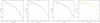 |
Fig. 12 Same as Fig. 11 for 10 Myr CSF models. |
| In the text | |
|
Fig. 13 Number of ionising photons per second as a function of age for population synthesis models. The upper left (upper right, lower left, lower right) panel is for H I (He I, He II, Ne II). Solid (dashed) lines are burst (CSF) models. Grey lines are for BPASS models that do not include VMSs, i.e. the models we use for stars with masses below 100 M⊙. |
| In the text | |
|
Fig. 14 Ionising photon efficiency as a function of age. Different colours are used for different metallicities and assumption regarding VMS mass-loss rate, as is explained in the upper right corner of the figure. Solid (dashed) lines are for burst (CSF) models that include nebular continuum emission. |
| In the text | |
|
Fig. 15 Comparison between burst population synthesis models including VMSs up to 225 M⊙ and the observed UV spectrum of the super star cluster in II Zw 40. All models are for Z = 0.2 Z⊙. Ages range from 0 to 2.5 Myr from top to bottom. The left (right) panels correspond to models without (with) metallicity scaling of the VMS mass-loss rates. |
| In the text | |
|
Fig. 16 Comparison between burst population synthesis models including VMSs up to 225 M⊙ to the observed UV spectrum of cluster A in II Zw 40 (black line). All models are for Z = 0.2 Z⊙ that is close to the metallicity of the cluster. Ages range from 0 to 2.5 Myr and are colour-coded as indicated in the top panel. The top (bottom) panel corresponds to models without (with) metallicity scaling of the VMS mass-loss rates. The vertical black lines indicate the Galactic nebular C IV absorption. |
| In the text | |
|
Fig. 17 Comparison between burst population synthesis models including VMSs up to 225 M⊙ and the observed UV spectrum of MrK71-A (black line). Top (bottom) models are for Z = 0.2 (0.1) Z⊙. In each panel ages range from 0 to 2.5 Myr from top to bottom. The left (right) panels correspond to models without (with) metallicity scaling of the VMS mass-loss rates. |
| In the text | |
|
Fig. 18 Comparison between Z = 0.2 Z⊙ CSF population synthesis models including VMSs up to 225 M⊙ and the observed UV spectrum of SB 126 (black line). Left (right) panels show models without (with) metallicity scaling of the VMS mass-loss rates. |
| In the text | |
|
Fig. 19 Comparison between the spectrum of the initial CSF population synthesis models at 10 Myr (black line) and the spectrum of a test model in which the contribution of evolved phases of evolution is included (red line). The left (right) panel is for Z = 0.1 (0.01) Z⊙. |
| In the text | |
|
Fig. 20 Ratio of He II to H I ionising photons fluxes as a function of age. The dashed (dash-dotted) lines correspond to CSF models in which the advanced phases of evolution are included (not included). In burst models these advanced phases are shown at 2.625 and 2.750 Myr. Blue (orange) lines are for Z = 0.1 (0.001) Z⊙. |
| In the text | |
|
Fig. B.1 Synthetic UV (bottom) and optical (top) spectra of the 200 M⊙ models at Z = 0.2 Z⊙. The left (right) panels correspond to models without (with) metallicity scaling of mass-loss rates. |
| In the text | |
|
Fig. B.2 Synthetic UV (bottom) and optical (top) spectra of the 200 M⊙ models at Z = 0.01 Z⊙. The left (right) panels correspond to models without (with) metallicity scaling of mass-loss rates. |
| In the text | |
Current usage metrics show cumulative count of Article Views (full-text article views including HTML views, PDF and ePub downloads, according to the available data) and Abstracts Views on Vision4Press platform.
Data correspond to usage on the plateform after 2015. The current usage metrics is available 48-96 hours after online publication and is updated daily on week days.
Initial download of the metrics may take a while.